QUANTITATIVE FINANCE RESEARCH CENTRE QUANTITATIVE F
INANCE RESEARCH CENTRE
QUANTITATIVE FINANCE RESEARCH CENTRE
Research Paper 272 February 2010
Option Valuation in Multivariate SABR Models Jörg Kienitz and Manuel Wittke
ISSN 1441-8010 www.qfrc.uts.edu.au
Option Valuation in Multivariate SABR
Models
- with an Application to the CMS Spread -
Jorg Kienitz∗and Manuel Wittke†
February 17, 2010
Abstract
We consider the joint dynamic of a basket of n-assets where each asset itself follows
a SABR stochastic volatility model. Using the Markovian Projection methodology we
approximate a univariate displaced diffusion SABR dynamic for the basket to price
caps and floors in closed form. This enables us to consider not only the asset corre-
lation but also the skew, the cross-skew and the decorrelation in our approximation.
The latter is not possible in alternative approximations to price e.g. spread options.
We illustrate the method by considering the example where the underlyings are two
constant maturity swap (CMS) rates. Here we examine the influence of the swaption
volatility cube on CMS spread options and compare our approximation formulae to
results obtained by Monte Carlo simulation and a copula approach.
JEL Classification: C63, G12, G13
Keywords: SABR, CMS Spread, Displaced Diffusion, Markovian Projection, Gyongy
Lemma
∗Deutsche Postbank AG, Head of Quantitative Analysis, Friedrich-Ebert-Allee 114-126, 53113 Bonn,[email protected]
†University of Bonn, BWL 3 - banking and finance, Adenaueralle 24-32, 53113 Bonn, [email protected]. Many thanks to the University of Technology, Sydney and especially to Erik Schlogl, for the supportto complete this work.
1
1 Introduction and Objectives
To value financial instruments taking into account the whole volatility cube can be done by
applying a model with stochastic volatility. This approach gained popularity over the last
years. One popular model for forward price processes and therefore heavily used in the fixed
income market is the SABR model of Hagan et al. [2003]. This model assumes that the
forward price process of an asset evolves under a stochastic volatility process correlated with
the forward price process. One of the major advantages of the SABR model in comparison
to other models with stochastic volatility is, that an approximation of a strike and time to
maturity dependent volatility function exists. This approximation can be plugged into the
well-known Black [1976] formula to calculate an arbitrage-free price.
In the setting of a basket of forward price processes, an option on the basket can only be
valued analytically by the formula of Margrabe [1978] in the case of two assets and a zero
strike. For higher dimensions the arbitrage-free price needs to be computed numerically. One
numerical method suited to these kind of problem is the Monte Carlo simulation. But in the
case of stochastic volatility, this procedure can be very time consuming. This is acceptable
if only an arbitrage-free price is be computed, but it is a major problem if the concern is the
calibration of a model to market prices. Therefore, approximation formulae for the contracts
to be calibrated to should be available.
The Markovian Projection is a method introduced to quantitative finance by Piterbarg [2006]
which applies the results by Gyoengy [1986]. The approximation is in the sense of the ter-
minal distribution a basket of diffusions by a univariate diffusion. This method is capable to
incorporate stochastic volatility models with a correlation structure between all stochastic
variables and has been applied by Antonov and Misirpashaev [2009] to project the spread
of two Heston diffusions. Using the case of multivariate SABR diffusions we show, how
the basket can be approximated by a displaced diffusion model of Rubinstein [1983] with
a SABR style stochastic volatility. Given the approximated SDE, caps/floors on a basket
of n-assets can be valued in closed form taking into account the volatility cube and a full
correlation structure. As a special case we consider the Geometric Brownian Motion and the
Constant Elasticity of Variance.
A liquid financial instrument in the fixed income market that depends on two correlated for-
ward price processes is the CMS spread option. The contracts payoff depends on the spread
of two CMS rates with different tenors. A CMS rate is a swaprate paid in one installment.
Its name origins from constant maturity swaps.
Regarding the valuation of spread options with nonzero strike several approximations and
simulations are discussed in the related literature. Using deterministic volatility the valua-
2
tion can be done by a semi-analytic conditioning technique, see Belomestny et al. [2008] or
in a swap market model or a displaced diffusion swap market model by Monte Carlo simula-
tion as shown by Leon [2006] and Joshi and Yang [2009]. Solutions for stochastic volatility
models are given by Dempster and Hong [2000] who extended the FFT method to spread
options, Antonov and Arneguy [2009] and Lutz and Kiesel [2010] who consider a stochastic
volatility LIBOR Market Model and approximations to the CMS rate as well as numerical
integration methods.
One approach in a SABR framework is to use a Gaussian copula with the margins being
SABR processes as shown by Berrahoui [2004] and Benhamou and Croissant [2007]. The
advantage of our proposed method using the Markovian Projection is that we can include
a rich correlation structure and derive a closed form solution which can be extended to the
n-asset case.
Concerning the valuation of products dependent on CMS rates, the expected value of a
CMS rate under a forward measure is its forward starting value and a convexity correction
independent of the chosen pricing model. This convexity correction can be computed by
an analytical approximation as discussed in Lu and Neftci [2003] or by using a replication
portfolio of European swaptions as proposed by Hagan [2003]. In the case of a Markovian
projected spread diffusion the convexity correction can be approximated by the difference of
the original CMS convexity corrections under a so-called spread measure.
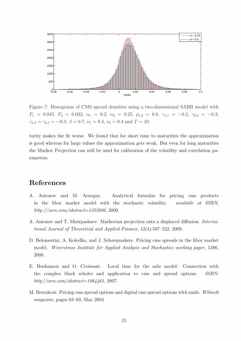
Numerical results for CMS spread options show, that the Markovian Projection of multivari-
ate SABR diffusions is a good approximation which for example can be used for volatility
and correlation calibration. For a liquid range of strike prices from 0 to 100 bp the model
prices lie close to the results obtained by Monte Carlo simulation and even outperform a
copula approach. But there are parameter sets for which the approximation is less accurate.
This is for instance the case for a large time to maturity, which rarely occurs in practical
applications.
Concerning the properties of a CMS spread option, the numerical studies show a signif-
icant influence of the swaption volatility cube and the correlation between the stochastic
correlation parameters on the options price. The final issue cannot be modeled by previous
mentioned approximations.
The paper is structured as follows. In Section 2 we first describe the multivariate SABR and
the SABR style displaced diffusion model. In a second step the approximated Markovian
Projection is computed for the general case of a n-dimensional basket. Section 3 applies the
results to the special case of a CMS spread option, where also the convexity correction of
CMS rates and a copula approach are presented. The accuracy of the suggested approxi-
3
mations and the properties of CMS spread options are illustrated in Section 4 by numerical
examples. Section 5 is the conclusion.
2 Model
One problem encountered when modeling derivatives like swaptions in a Swap Market Model
and therefore using the Black [1976] formula is, that the market prices for swaptions cannot
be obtained with a constant volatility parameter as the model demands. Instead the volatility
tends to rise if the option is out of the money. This results in the so called volatility smile
describing the fact that implied Black volatility is strike depended. The problem with implied
volatility is that it needs to be interpolated from market data and more important the
assumption of a different model for each strike. With this in mind Dupire [1994] proposed
the local volatility model. The advantage of this approach is that the model perfectly
replicates the current market situation. But the approach behaves poorly in forecasting
future dynamics and option pricing is not possible in closed form. An alternative suggested
by Hagan et al. [2003] is the so called SABR model where a forward price process is modeled
under its forward measure using a correlated stochastic volatility process. Assuming the
usual conditions, the diffusion of a forward price S(t) is given by:
dS(t) = α(t)S(t)βdW (t)
dα(t) = να(t)dZ(t)
S(0) = s
α(0) = α0
〈dW (t), dZ(t)〉 = γW,Zdt
with α(t) the stochastic volatility, ν the volatility of the volatility and W (t) and Z(t) corre-
lated Brownian Motions. γW,Z is the correlation of the forward price and volatility process
under an appropriate forward measure. β can be chosen to further specify the distribution
of the forward price process. For example β = 1 constitutes a lognormal distribution and
β = 0 a normal distribution under the assumption of a deterministic volatility and is also
called the backbone of the diffusion process.
For a fixed maturity the parameters can be calibrated to all strikes where market data of op-
tion volatilities is available. This is the so called volatility cube as shown in figure (1) for the
swaption market. One major advantage of the model is that there exists an approximation
formula to implied Black [1976] volatility using the SABR parameters. Therefore option
prices can be calculated using the well known pricing framework but taking into account
the volatility cube using a strike dependent volatility function. Today the SABR model has
become one standard model in the financial industry because of the described properties and
4
Figure 1: Implied 10y Swaption Volatilities of 18.09.2009.
easy application.
Basket options are options where the underlying is a basket of assets. Let N be the number
of different correlated assets, denoting the weights by εi, i = 1, . . . , N . For instance N = 2,
ε1 = 1 and ε2 = −1 constitutes a spread. To compute the arbitrage-free price of a basket
option with the underlyingN∑
i=1
εiSi
we propose to use a multidimensional SABR model.
Definition 2.1 A multidimensional SABR diffusion is given as follows. For each asset Si(t)
with i = {1, . . . , N} let:
dSi(t) = αi(t)Si(t)βidWi(t)
dαi(t) = νiαi(t)dZi(t)
Si(0) = s0i
αi(0) = α0i
〈dWi(t), dWj(t)〉 = ρijdt
〈dWi(t), dZj(t)〉 = γijdt
〈dZi(t), dZj(t)〉 = ξijdt. (1)
where ρij is the correlation between the Brownian Motions driving the asset price processes,
γij the cross-skew and ξij the so called decorrelation between the stochastic volatilites.
5
The multidimensional SABR process models the dependency between all factors, which will
be further examined in section (4).
A major problem when valuing basket options is that only for βi = 0 i = 1, . . . , N , the case of
a normal distributed asset and deterministic volatility νi = 0 i = 1, . . . , N , the distribution of
the basket is known and option prices can be computed in closed form. For the special case of
two assets with β1,2 = 1 and a zero strike a solution is given by the Margrabe [1978] formula.
But for nonzero strikes and more than two assets under a SABR stochastic volatility only
numerical methods and semi-analytic approximation formulae are known. In the following,
we extend the framework by a projected multivariate SABR diffusion which can applied to
the n-assets case.
2.1 Markovian Projection
An approximation method introduced to quantitative finance by Piterbarg [2006] is the
Markovian Projection. It applies the results of Gyoengy [1986] to project multidimensional
processes onto a reasonable simple process. Using this methodology we project a multidi-
mensional SABR diffusion process onto a one-dimensional displaced diffusion SABR model.
Formally, we approximate the diffusion of the basket with a displaced diffusion with stochas-
tic volatility. The latter results using the Markovian Projection imply β = 1 and therefore
we restrict ourselves to this special case.
Definition 2.2 A displaced SABR diffusion for β = 1 is given by:
dS(t) = α(t)F (S(t))dW (t)
dα(t) = να(t)dZ(t)
〈dW (t), dZ(t)〉 = γdt
with F (S(t)) = p + q(S(t)− S(0))
p = F (S(0))
q = F (S(0)) (2)
where γ denotes the correlation between the forward price and the volatility process.
A displaced diffusion is a reasonable choice, since in case of spread options negative realiza-
tions of the spread must have positive probabilities.
The key result to approximate the multidimensional model of Eq. (1) using a single SABR
like diffusion, Eq. (2), is the following result derived by Gyoengy [1986].
Lemma 2.1 Let X(t) be given by
Let dX(t) = α(t)dt + β(t)dW (t), (3)
6
where α(.), β(.) are adapted bounded stochastic processes such that Eq. (3) admits a unique
solution. Define a(t, x), b(t, x) by
a(t, x) = E[α(t)|X(t) = x]
b2(t, x) = E[β2(t)|X(t) = x]
Then, the SDE
dY (t) = a(t, Y (t))dt + b(t, Y (t))dW (t),
Y (0) = X(0),
admits a weak solution Y (t) that has the same one-dimensional distribution as X(t).
Using Lemma 2.1, the multidimensional model of Eq. (1) is projected onto the displaced
SABR diffusion of Eq. (2). The computations involve approximations, which we explain in
detail in the proof of the following Theorem.
Theorem 2.1 The dynamics of a basket of assets following a multivariate SABR model,
Eq. (1), is approximated by:
dS(t) = u(t)F (S(t))dW (t)
du(t) = ηu(t)dZ(t)
S(0) = s0
u(0) = 1
〈dW (t), dZ(t)〉 = γdt
F (S(0)) = p
F (S(0)) = q.
Proof
The approximation is computed in several steps. First, we rewrite the original SABR diffu-
sion of Eq. (1) as a single diffusion with stochastic volatility driven by a Brownian Motion.
To preserve the starting values of the process we rescale the volatility of Eq. (1) by:
ui(t) =αi(t)
αi(0)
ϕ(Si(t)) = αi(0)Si(t)βi
⇒ dSi(t) = ui(t)ϕ(Si(t))dWi(t).
Furthermore, we assume βi = β and introduce the notation:
ϕ(Si(0)) = pi = αi(0)Si(0)β
ϕ (Si(0)) = qi = αi(0)βiSi(0)β−1.
7
In the SABR setting we thus choose the local volatility to be f(x) = xβ but other choices
are possible. Then, we replace the latter expressions by pi = f(Si(0)) and qi = f ′(Si(0)).
First, using the SDE for the individual assets, we find:
dS(t) =N∑
i=1
εidSi(t)
=N∑
i=1
εiui(t)ϕ(Si(t))dWi(t).
Choosing the Brownian Motion such that:
dW (t) = σ−1(t)N∑
i=1
εiuiϕ(Si(t))dWi(t)
we have the representation:
dS(t) = σ(t)dW (t)
with εij = εi · εj and σ(t) given by:
σ2(t) =N∑
i=1
εiu2i ϕ
2(Si(t)) + 2N∑
i<j
εijρijuiujϕ(Si(t))ϕ(Sj(t)).
Under this specification, the Levy characterization gives that W (t) is a Brownian Motion.
To apply the result of Gyoengy [1986] we need to compute the variance of Eq. (2) on which
Eq. (1) is to be projected. We compute u2(t) as:
u2(t) =1
p2
(2
N∑i<j
pipjui(t)uj(t)ρijεij +N∑
i=1
p2i ui(t)
2
)(4)
with p =
√√√√N∑
i=1
p2i + 2
N∑i<j
ρijpipjεij. (5)
The factor 1/p is necessary to ensure u(0) = 1. For t = 0 we find σ(0) = p.
Now, we are in a position to apply the result of Gyongy. With the notation of Lemma 2.1
we set b(t, x) = E[σ2(t)|S(t) = x] and on the other hand b(t, x) = E[u2(t)|S(t) = x] · F 2(x).
Thus, we have
F 2(x) =E[σ2(t)|S(t) = x]
E[u2(t)|S(t) = x]. (6)
To compute the conditional expectations of the nominator and the denominator we observe
that σ2(t) and u2(t) are linear combinations of the form:
fij(t) = ϕ(Si)ϕ(Sj)ui(t)uj(t)
gij(t) =pipjui(t)uj(t)
p2(7)
8
and can be represented as follows:
σ2(t) =N∑
i=1
fii(t) + 2N∑
i<j
fij(t)ρijεij
u2(t) =N∑
i=1
gii(t) + 2N∑
i<j
gij(t)ρijεij.
To compute the conditional expectation, a first order Taylor expansion leads to
fij ≈ pipj
(1 +
qi
pi
(Si(t)− Si(0)) +qj
pj
(Sj(t)− Sj(0)) + (ui(t)− 1) + (uj(t)− 1)
)(8)
and
gij ≈ pipj
p2(1 + (ui(t)− 1) + (uj(t)− 1)) . (9)
Thus, to compute the conditional expectations of Eq. (6) we need simple expressions for
E[Si(t)− Si(0)|S(t) = x]
E[ui(t)− 1|S(t) = x]. (10)
To find a simple formula we apply a Gaussian approximation to compute the expected values.
The Gaussian approximation is a simple but reasonable approximation and is given by:
dSi(t) ≈ dSi(t) = pidWi(t),
dui(t) ≈ dui(t) = νidZ(t),
dS(t) ≈ dS(t) = pdW (t),
¯dW = p−1
N∑i=1
piεidWi(t).
We have the correlation structure:
〈dW (t), dWi(t)〉 = p−1
N∑j=1
pjεjρjidt = ρidt
〈dW (t), dZi(t)〉 = p−1
N∑j=1
pjεjγjiρj+Ndt = ρi+Ndt.
The expected values can now be computed. We have:
E[Si(t)− Si(0)|S(t) = x] =〈Si(t), S(t)〉〈S(t), S(t)〉 (x− S(0)) = piρi
x− S(0)
p
and
E[ui(t)− 1|S(t) = x] = νiρi+Nx− S(0)
p.
9
Using these expressions we compute F (t, x). Denoting the coefficient appearing in the de-
nominator by Ad and the numerator by Au we find:
F 2(x) =E[σ2(t)|S(t) = x]
E[u2(t)|S(t) = x]≈ p2 + Au(x− S(0))
1 + Ad(x− S(0))(11)
with:
Au =2
p
{N∑
i=1
p2i (qiρi + νiρi+N)
+N∑
i<j
εijρijpipj(qiρi + qjρj + νiρi+N + νjρj+N)
},
Ad =2
p3
{N∑
i=1
p2i νiρi+N
N∑i<j
εijρijpipj(νiρi+N + νjρj+N)
}.
Given these solutions F (S(0)) and F (S(0)) are given by:
F (S(0)) = p F (S(0)) = q
with p given by Eq.(5) and q given by:
q =
∑Ni=1
(p2
i qiρi +∑N
i6=j piqiρijρiεijpj
)
p2.
Finally, we need to derive a SABR like diffusion for the stochastic volatility and apply the
Ito formula to derive the SDE for u(t). Only using first order approximations and replacing
the quotientsui(t)uj(t)
u2(t)with the expected value,
E[u2
i (t)
u2(t)
]= E
[ui(t)uj(t)
u2(t)
]= 1
we find:
du(t)
u(t)=
1
p2
N∑i=1
(p2
i
u2i
u2+
N∑
i6=j
εijρijpipjuiuj
u2
)νidZi(t)
=1
p2
N∑i=1
(p2
i +N∑
i6=j
εijpipj
)νidZi(t). (12)
For more accurate approximations we may keep the higher order terms. This results in
a more complex expression and drift terms. In this case we can apply the results for the
λ-SABR model, see Labordere [2005].
Thus, by computing the (simple) approximation we obtain a SDE for u(t) which we denote
by:
du(t) = ηu(t)dZ(t).
10
For the Brownian Motion Z(t) we have
dZ(t) =
∑Ni=1
(p2
i νi +∑N
i 6=j εijρijpipjνi
)dZi(t)
ηp2,
η2 = V ar
∑Ni=1
(p2
i νi +∑N
i6=j εijρijpipjνi
)dZi(t)
p2
with η such that Z(t) scales to 〈Z(t)〉 = t. We determine the correlation between the
dynamics of the forward price process and the stochastic volatility as:
γ =〈dW (t), dZ(t)〉
dt
≈ 〈dW (t), dZ(t)〉dt
=1
ηp3
N∑i=1
N∑
k=1
(p2
i νi +N∑
i6=j
εijρijpipjνi
)pkεkγik. (13)
End of Proof
For νi = 0, i = 1, . . . , N we end up with the projection of CEV diffusions since all stochastic
volatility and cross correlation terms in the calculation of q cancel out. For ν = 0 and
βi = 1, i = 1, . . . , N the basket of SABR diffusion even simplifies to a basket of Geometric
Brownian Motions.
In Figure (2) the densities for the spread of Geometric Brownian Motions are plotted. We
compare the application of Markovian Projection and of Monte Carlo simulation. The neg-
ative values, especially for a maturity of 10 years, are modeled appropriately. The influence
of the difference between the Markovian Projection and the Monte Carlo simulation on the
price of options in the case of SABR diffusions is discussed in Section (4).
2.2 Pricing
We now apply our method to the valuation of CMS caplets resp. floorlets. In the above
setting we linearize F (S(t)) as:
F (S(t)) = (S(t) + a)q
with a =p
q− S(0).
This is to rewrite the projected SDE as a displaced diffusion. Using the implied SABR
volatility function σSABR, the solution of the projected SDE can be written as an asset in
a Black [1976] framework and therefore the closed form displaced diffusion formula can be
11
−0.01 0 0.01 0.02 0.03 0.04 0.050
0.5
1
1.5
2
2.5
3
3.5x 10
4
Spread; T=1
Monte CarloMarkovian Projection
−0.02 0 0.02 0.04 0.06 0.08 0.1 0.120
0.5
1
1.5
2
2.5
3
3.5x 10
4
Spread; T=10
Monte CarloMarkovian Projection
Figure 2: Density of the spread of two Geometric Brownian Motions using a Monte Carlo
simulation and a Markovian Projection onto a displaced diffusion.
used. But the expectation of the payoff has to be taken under the T forward measure and
since solution of the asset is lognormal distributed we can formulate the pricing equation as:
CMScaplet = B(0, T )ET [S(T )−K]+
= B(0, T )ET [S(T ) + a− (K + a)]+
= B(0, T ){(EP T [S(T )] + a)N(d1)− (K + a)N(d2)}
with d1/2 =ln
(E
PT [S(T )]+a
K+a
)± 1
2σ2
SABR(τ − t)
σSABR
√(τ − t)
12
The volatility function is given by:
σSABR =α
(fK)(1−β)/2{
1 + (1−β)2
24log2f/K + (1−β)4
1920log4f/K
}(
z
x(z)
)
{1 +
[(1− β)2
24
α2
(fK)1−β+
1
4
ρβνα
(fK)(1−β)/2+
2− 3ρ2
24ν2
]t
}
with z =ν
α(fK)(1−β)/2 log f/K,
f = EP T [S(T )],
α = q
and x(z) = log
{√1− 2ρz + z2 + z − ρ
1− ρ
}.
Therefore, the pricing depends on the chosen measure of the projected SDE. If the SDE is
given with respect to the same forward measure, the pricing equation is solved by setting
EP T [S(T )] = S(0). This is in general not the case if different swaprates are projected onto
a SDE. The solution in this case is its forward value and a convexity correction as discussed
in Section (3). This is the case for a CMS spread option.
3 Application to CMS
Constant maturity swaps (CMS) are interest rate swaps where the fixed leg pays a swaprate
with a constant time to maturity at every payment date. These are liquid financial instru-
ments that allow to take positions on future long term rates due to the constant maturity
of the fixed leg payments. The underlying swaprate are also an important building block
of structured products in todays fixed income markets. Such products incorporate a CMS
structure with payment dates similar to a swap but use the constant maturity swaprates as
an underlying for embedded options. Common CMS payments in fixed income structured
products are
• Capped / Floored CMS Coupons, (CMSN),
• Capped / Floored CMS Spread Coupons, (CMSM − CMSN) and
• Capped / Floored CMS Swing Coupons, (CMSN − CMSO)− (CMSM − CMSN).
The subscripts indicate that the underlying CMS yields are for different time to maturity
with M > N > O. The structure of CMS spread and swing options allow to express views on
future changes of the shape of the yield curve. Particularly, steepening or flattening is traded
using spread options and the curvature of the yield curve using swing options. Therefore,
such options can be used as hedges of interest rate correlation risk.
13
Concerning the pricing of CMS options, regardless of the chosen model, an expectation of
a CMS rate at the maturity of the option needs to be computed. Since the CMS rate at
maturity τ given by yN(τ) = 1−B(τ,τ+N)∑Ni=1 B(τ,τ+i)
is payed in one installment and not as a standard
swap we can not choose the annuity as a numeraire. Instead we choose a forward risk adjusted
measure which coincides with the options maturity and the CMS rate is not a martingale
under this measure. To compute the expectation of the CMS rate one has to incorporate
a convexity adjustment to the forward swaprate. For a Geometric Brownian Motion this
convexity adjustment can be approximated analytically, see Lu and Neftci [2003].
Since we assume stochastic volatility we have to incorporate this into computation of the
convexity adjustment. One method proposed by Hagan [2003] is the replication of CMS
caplet by a portfolio of European swaptions in the SABR model
CMS caplet =B(t, τ)
A(t)
{[1 + f (K)]C(K) +
∫ ∞
K
C(x)f´ (x)dx
}
with A(t) = Annuity,
f(x) = Weightfunction,
C(x) = Payer Swaption with K = x. (14)
Therefore, replicating CMS caplets uses all market information by a static hedge portfolio
consisting of plain-vanilla swaptions. Using the cap-floor parity
yN(t) = yN(t, τ) + CMS caplet− CMS floorlet︸ ︷︷ ︸convexity correction
(15)
the convexity adjusted CMS rate yN(t) can be computed by the forward starting swaprate
and a portfolio of payer and receiver swaptions.
3.1 CMS Spread Options
To give comparable numerical results for CMS options priced by the Markovian Projetion
approach in a multidimensional SABR model we restrict the implementation to the case of
a CMS spread option. The payoff at maturity τ is as follows:
max{yM(τ)− yN(τ)−K, 0}
with M ≥ N .
The special case of zero strike options, K = 0, can be solved analytically using the formula
for exchange options, see Margrabe [1978]. For K 6= 0 an analytical solution is only feasible
if the spread is modeled as a normal distributed random variable
yM(τ)− yN(τ) = y(τ)
with dy(t) = σdW (t).
14
This framework is too simple to consistently price CMS Spread Options since implicitly a
perfect correlation is assumed. And it is also not taking into account the smile and the
skew effects. The market quotes spread options by their implied normal volatilities such as
swaptions are quoted by their implied Black volatility.
In the following we present the copula approach of Berrahoui [2004] and Benhamou and
Croissant [2007] and show how to project the spread onto a displaced diffusion using a
SABR model. Then, we price a CMS spread option using both approaches.
3.2 Approximation of the Correlation Structure
One way to approximate spreads in a SABR framework is the copula approach which we
review in the following. The idea is that the payoff of spread options with two correlated
price processes can be decomposed into a portfolio of digital options and is given as:
max{yM(τ)− yN(τ)−K, 0} =
∫ ∞
0
1[yM (τ)>x+K]1[yN (τ)<x]dx.
Now taking the discounted expectation under the risk adjusted measure P τ , the fair value
can be computed by using numerical integration:
CMSspreadcaplet = B(t, τ)
∫ ∞
0
P τ (yM(τ) > x + K, yN(τ) < x)dx. (16)
The joint probability function P τ (. . .) can be computed using a Gaussian copula with the
SABR margins. The procedure consists of two steps. First, we have to compute the margins
of the SABR distributions and then have to map the quantiles them onto a lognormal
distribution as shown in Figure (3). The second step uses the Gaussian copula to obtain
the joint probability function. As stated above, we first need the margins PSABR(yi(τ) > xi)
1 2 3 4 5
0.2
0.4
0.6
0.8
1.0
1.2
1.4
Figure 3: Quantile mapping of a SABR distribution onto a lognormal distribution
which can be computed numerically or replicated using digital options. To map the SABR
15
distribution onto a lognormal for a given SABR quantile we compute the equivalent Black
quantile and solve for the value xi:
PSABR(yi(τ) > xi) = PBlack(yi(τ) > xi|σ = σSABR).
The joint probability distribution is computed using a Gaussian copula and correlation
〈dWN(t), dWM(t)〉 = ρdt. It is given by:
P (yM(τ) > x + K, yN(τ) < x) ≈ N(d2)−N2(d1, d2, ρ) (17)
with di =1
σSABR
√τ
(ln
(xi
yM/N(t)
)+
1
2σ2
SABRτ
).
To compute the approximated arbitrage-free price of the CMS spread option we need to
apply Eq. (17) and substitute it into Eq. (16). Finally we use a numerical integration
method.
We can alter the correlation structure using a different copula, for instance the t-copula with
heavier tail dependence. As will be shown in Section (4) the copula approach prices the
CMS Spread Options fairly accurate, but there are still some drawbacks of this method:
• The copula method is static and we have no process of the spread dynamic.
• The numerical integration is time consuming.
• The decorrelation and cross skews are assumed to be uncorrelated.
• The methodology cannot be extended to CMS options with more than two CMS rates.
3.3 Approximation of the Spread Diffusion
In this subsection we apply the general results obtained in the previous section to the case
of a CMS spread option. The guiding idea is to compute a SDE for the spread dynamics
which approximates the joint SABR dynamics at maturity using the full correlation structure
including decorrelation and cross skew. It also captures the volatility smile as it can be seen
in Figure (4) for some given parameters.
Theorem 3.1 The dynamics of the spread can be approximated by
dS(t) = u(t)F (S(t))dW (t)
du(t) = ηu(t)dZ(t)
with u(t) and p(t) given by Eq. (4) with N = 2 and the function F (.) satisfying:
F (S(0)) = p F (S(0)) = q
16
0 0.005 0.01 0.015 0.02 0.025 0.03 0.035 0.04 0.045 0.052.2
2.25
2.3
2.35
2.4
2.45
2.5x 10
−3
Strike
Vol
atili
ty
Markov Projection
Figure 4: Strike dependent implied CMS spread call volatilities of prices obtained by a
Markov Projection with F1 = 0.045, F2 = 0.032, α1 = 0.2, α2 = 0.25, ρ1,2 = 0.8, γ1,1 = −0.2,
γ2,2 = −0.3, γ1,2 = γ2,1 = −0.3, ξ1,2 = 0.75, β = 0.7, ν1 = 0.4, ν2 = 0.4 and T = 10.
with
q =p1q1ρ
21 − p2q2ρ
22
p,
η =
√1
p2[(p1ν1ρ1)2 + (p2ν2ρ2)2 − 2ξ12p1ν1ρ1p2ν2ρ2].
and
γ =1
ηp2
(p2
1ν1ρ1γ11 + p22ν2ρ2γ22 − p1p2ν2ρ2γ21 − p1p2ν1ρ1γ12
).
Proof
We consider the dynamics of Eq. (1) and compute the diffusion for the spread taking
N = 2, ε1 = 1 and ε2 = −1. Since we model swaprates with different tenor structures, we
cannot model them as driftless processes under the same forward measure P T since they
obtain a drift term µi. In fact, they are driftless under their own annuity measure PAi .
Therefore, we change both measures to a so-called spread measure P S under which their
spread SDE is driftless and given by:
dS(t) = dS1(t)− dS2(t)
= (µ1dt + u1(t)ϕ(S1(t))dW T1 (t))− (µ2dt + u2(t)ϕ(S2(t))dW T
2 (t))
!=
σ(t)dW S(t)
with:
dW S(t) =1
σ(t)
(u1(t)ϕ(S1(t))dW S
1 − u1(t)ϕ(S2(t))dW S2
)
σ2(t) = u21(t)ϕ(S1(t))
2 + u22(t)ϕ(S2(t))
2
− 2ρ12u1(t)u2(t)ϕ(S1(t))ϕ(S2(t)). (18)
17
In a second step we compute the variance of the approximating SDE as given by Eq. (18):
u2(t) =1
p2
(p2
1u21(t) + p2
2u22(t)− 2ρ12p1p2u1(t)u2(t)
)
with p = σ(0) =√
p21 + p2
2 − 2ρ12p1p2.
At this point we have two representations for the spread SDE:
dS(t) = σ(t)dW S(t) and dS(t) = u(t)F (S(t))dW S(t).
With the first equation being the original spread SDE and the second one the approximating
SDE under the spread measure. We now have to compute the parameters of the approximat-
ing SDE that mimic the terminal one-dimensional distribution of the original SDE. Applying
the Gyoengy [1986] result, we have to choose F 2(t, x) such that:
F 2(x) =E [σ2(t)|S(t) = x]
E [u2(t)|S(t) = x]. (19)
To proceed, we use Eq. (7) to further simplify the notation. Then, we can compute the
volatilities:
σ2(t) = f11(t) + f22(t)− 2ρ12f12(t)
u2(t) = g11(t) + g22(t)− 2ρ12g12(t).
To be able to compute the conditional expectations, we use the first order Taylor approx-
imation as in Eq. (8) and Eq. (9). This reduces the problem to the computation of the
conditional expectations for Si(t) and ui(t), Eq. (10). To make the calculations more ex-
plicit we apply a Gaussian approximation. Using the approximation we can simplify the
conditional expectations as follows:
E[Si(t)− Si(0)|S(t) = x] = piρi(x− S(0))
p
and
E[ui(t)− 1|S(t) = x] = νiρi+2(x− S(0))
p.
This leads to a simple expression for the numerator and the denominator of equation (19):
E[σ2(t)|S(t) = x
] ≈ p2 + (x− S(0))Au
with Au =2
p
(p2
1(q1ρ1 + ν1ρ3) + p22(q2ρ2 + ν2ρ4)
−p1p2ρ12
(q1ρ1 + q2ρ2 + ν1ρ3 + ν2ρ4
)),
E[u2(t)|S(t) = x
] ≈ 1 + (x− S(0))Ad
with Ad =2
p3
(ν1p1(p1 − p2ρ12)ρ3 + ν2(p2 − p1ρ12)ρ3
).
18
We can compute the approximating SDE for S(t). To compute the dynamics of u(t), we
apply Eq. (12) to get:
du(t) =1
p2
(p2
1ν1u2
1
u2− ρ12p1p2ν1
u1u2
u2
)u(t)dZ1(t)
+1
p2
(p2
2ν2u2
2
u2− ρ12p1p2ν2
u1u2
u2
)u(t)dZ2(t)
⇔ du(t)
u(t)=
(p1ν1ρ1
pdZ1(t) +
p2ν2ρ2
pdZ2(t)
)
and we have the SDE by setting:
Z(t) =1
ηp
(p1ν1ρ1dZ1 − ρ2ν2ρ2dZ2
)
η2 =1
p2
[(p1ν1ρ1)
2 + (p2ν2ρ2)2 − 2ξ12p1ν1ρ1p2ν2ρ2
].
The correlation between the projected forward price process S(t) and its stochastic volatility
process u(t) can be computed using Eq. (13):
γ =1
ηp2
(p2
1ν1ρ1γ11 + p22ν2ρ2γ22 − p1p2ν2ρ2γ21 − p1p2ν1ρ1γ12
).
End of Proof
To compute the price of an option using the displaced diffusion model, the expectation of
the approximated spread at maturity needs to be computed. But the expectation is under
the forward measure, while the approximated spread is under the spread measure. This can
be solved by changes of measure and using the convexity adjustment, Eq. (15). Denoting by
Ai(t) the numeraire of the annuity measure PAi and by SN(t) the numeraire of the spread
measure the expectation can be computed:
EP T [S(T )]
= EP S
[S(T )
B(T, T )
SN(T )
SN(0)
B(0, T )
]
= S(0) + EP A1
[S1(T )
(B(T, T )
A1(T )
A1(0)
B(0, T )− 1
)]− EP A1
[S1(T )
(SN(T )
A1(T )
A1(0)
SN(0)− 1
)]
−EP A2
[S2(T )
(B(T, T )
A2(T )
A2(0)
B(0, T )− 1
)]+ EP A2
[S2(T )
(SN(T )
A2(T )
A2(0)
SN(0)− 1
)]
≈ {S1(0)− S2(0)}+ {convexity correction(S1)− convexity correction(S2)}.
The terms EP Ai
[Si(T )
(B(T,T )Ai(T )
Ai(0)B(0,T )
− 1)]
denote the convexity correction, see for instance
Hagan [2003], of the swapyield i which can be conducted by a replication portfolio within a
SABR framework. The difference:{
EP A1
[S1(T )
(SN(T )
A1(T )
A1(0)
SN(0)− 1
)]− EP A2
[S2(T )
(SN(T )
A2(T )
A2(0)
SN(0)− 1
)]}≈ 0
19
is approximated with a zero value, since the corrections due to the mismatch of the annuity
measures and the spread measure can be assumed to be close to zero with nearly identical
values for both expectations. Using convexity corrected swaprates the valuation of a CMS
spread caplet or floorlet is now possible.
4 Numerical Results
To illustrate the approximation in the case of a basket option using the Copula and the
Markovian Projection approach, we apply the results obtained in Section (3) for valuation
of spread options in a SABR model. Since the copula approach is as discussed only valid
for two underlying diffusions. As a benchmark we apply a Monte Carlo simulation for the
multivariate SABR model.
In the following we consider the parameters: F1 = 0.045, F2 = 0.032, α1 = 0.2, α2 = 0.25,
ρ1,2 = 0.8, γ1,1 = −0.2, γ2,2 = −0.3, γ1,2 = γ2,1 = −0.3, ξ1,2 = 0.75, β = 0.7, ν1 = 0.4,
ν2 = 0.4 and T = 10.
First, we study the effect of changing the time to maturity and strike prices on the option
prices. To this end we price CMS spread calls and change the time to maturity and the
strike prices. In Figure (5) the numerical results of the Copula approach, the Markovian
Projection approach and a Monte Carlo simulation are plotted.
It can be seen that the fit of the Copula approach and the Markovian Projection approach
is reasonable good for five years to maturity. For ten years to maturity the goodness of
the approximations is still good but the reference prices of the Monte Carlo simulation are
clearly not in line with them. Both prices lie strictly below the Monte Carlo simulation but
the Markovian Projection outperforms the Copula approach. As a result the approximations
depend on the time to maturity and therefore should for longer times to maturity only be
used with care for the calibration to market prices.
To examine the influence of the swaption volatility cube on the prices of CMS spread op-
tions we consider the strike dependent prices in Figure (6). For a SABR model calibrated
to market data of a given strike range and a GBM using the ATM volatility we consider
their price differences. It can be seen that the influence is significant. Therefore, it must be
incorporated for longer times to maturity.
One advantage of the Markovian Projection in comparison to the Copula approach is that
the cross skew and the decorrelation are incorporated into the pricing. The influence of
these parameters on the arbitrage-free price is significant as shown in Figure (8). There,
arbitrage-free prices are plotted in dependence of the strike prices for different parameter
20
0 0.001 0.002 0.003 0.004 0.005 0.006 0.007 0.008 0.009 0.0160
70
80
90
100
110
120
130
140
150
Strike; T=5
Pric
e
Markovian ProjectionCopulaMonte Carlo
0 0.001 0.002 0.003 0.004 0.005 0.006 0.007 0.008 0.009 0.0180
90
100
110
120
130
140
150
160
170
Strike; T=10
Pric
e
Markovian ProjectionCopulaMonte Carlo
Figure 5: Strike dependent CMS spread call prices of a Markov Projection, a Copula and
a Monte Carlo simulation with F1 = 0.045, F2 = 0.032, α1 = 0.2, α2 = 0.25, ρ1,2 = 0.8,
γ1,1 = −0.2, γ2,2 = −0.3, γ1,2 = γ2,1 = −0.3, ξ1,2 = 0.75, β = 0.7, ν1 = 0.4, and ν2 = 0.4.
The first Figure is plotted with T = 5 and the second with T = 10.
values. The decorrelation parameter ξ shifts the prices parallel with a negative decorrelation
leading to the lowest prices. This is due to the dependency of the spread distribution to the
decorrelation. A lower decorrelation parameter shifts mass into the tails of the distribution.
This comes clear by considering Figure (7) where two histograms of a SABR spread density
are plotted for different values of ξ. If we change both cross skews γ = γ1 = γ2 simultaneously,
the divergence in prices is smaller than by changing the decorrelation ξ with a slightly twist.
As a result, if a multivariate SABR model is used to price baskets the decorrelation and
cross skew parameters have a significant influence on the price.
Since the Markovian Projection is an approximation which is less accurate for long times
to maturity, a proper valuation of a basket should in this case be done by a Monte Carlo
simulation using the Markovian Projection for calibration. But the calibration is numerically
very fast, since the Markovian Projection is an analytical approximation, while the Monte
21
0 0.001 0.002 0.003 0.004 0.005 0.006 0.007 0.008 0.009 0.0140
50
60
70
80
90
100
110
120
130
140
Strike, T=1
Pric
e
Stochastic VolatilitDeterministic Volatility
0 0.001 0.002 0.003 0.004 0.005 0.006 0.007 0.008 0.009 0.0180
90
100
110
120
130
140
150
160
Strike, T=10
Pric
e
Stochastic VolatilityDeterministic Volatility
Figure 6: Strike dependent CMS spread call prices using GBM (deterministic volatility) and
a SARR model (stochastic volatility) with F1 = 0.045, F2 = 0.032, α1 = 0.2, α2 = 0.25,
ρ1,2 = 0.8, γ1,1 = −0.2, γ2,2 = −0.3, γ1,2 = γ2,1 = −0.3, ξ1,2 = 0.75, β = 0.7, ν1 = 0.4 and
ν2 = 0.4.
Carlo simulation and the Copula approach are plain numerical methods.
5 Conclusion
We have presented the application of the Markovian Projection technique to the SABR
stochastic volatility model in multiple dimensions. As an example we have applied it to a
popular interest rate derivative, the CMS spread option that significantly depends on the
swaption volatility cube. The proposed technique takes into account all parameters modeling
the dependence structure such as the correlation of the underlying forward CMS rates, the
correlation between the rates and the volatility processes and the correlation between the
volatility processes.
We find a good match with results obtained using Monte Carlo simulation. However, there
are parameter sets where the fit is not reasonable. In particular changing the time to ma-
22
−0.08 −0.06 −0.04 −0.02 0 0.02 0.04 0.06 0.08 0.10
500
1000
1500
2000
2500
3000
3500
Strike
xi = 0.75xi = 0.0
Figure 7: Histograms of CMS spread densities using a two-dimensional SABR model with
F1 = 0.045, F2 = 0.032, α1 = 0.2, α2 = 0.25, ρ1,2 = 0.8, γ1,1 = −0.2, γ2,2 = −0.3,
γ1,2 = γ2,1 = −0.3, β = 0.7, ν1 = 0.4, ν2 = 0.4 and T = 10.
turity makes the fir worse. We found that for short time to maturities the approximation
is good whereas for large values the approximation gets weak. But even for long maturities
the Markov Projection can still be used for calibration of the volatility and correlation pa-
rameters.
References
A. Antonov and M. Arneguy. Analytical formulas for pricing cms products
in the libor market model with the stochastic volatility. available at SSRN,
http://ssrn.com/abstract=1352606, 2009.
A. Antonov and T. Misirpashaev. Markovian projection onto a displaced diffusion. Interna-
tional Journal of Theoretical and Applied Finance, 12(4):507–522, 2009.
D. Belomestny, A. Kolodko, and J. Schoenmakers. Pricing cms spreads in the libor market
model. Weierstrass Institute for Applied Analysis and Stochastics working paper, 1386,
2008.
E. Benhamou and O. Croissant. Local time for the sabr model: Connection with
the complex black scholes and application to cms and spread options. SSRN:
http//ssrn.com/abstract=1064461, 2007.
M. Berrahoui. Pricing cms spread options and digital cms spread options with smile. Wilmott
magazine, pages 63–69, May 2004.
23
0 0.02 0.04 0.06 0.08 0.1 0.12 0.14 0.16 0.18 0.20
50
100
150
200
250
300
Strike
Pric
e
Markov Projection with xi = 1Markov Projection with xi = 0Markov Projection with xi = −1
0 0.02 0.04 0.06 0.08 0.1 0.12 0.14 0.16 0.18 0.20
50
100
150
200
250
300
Strike
Pric
e
Markov Projection with gamma = 1Markov Projection with gamma = 0Markov Projection with gamma = −1
Figure 8: Strike dependent CMS spread call prices of a Markov Projection with F1 = 0.045,
F2 = 0.032, α1 = 0.2, α2 = 0.25, ρ1,2 = 0.8, γ1,1 = −0.2, γ2,2 = −0.3, γ1,2 = γ2,1 = −0.3,
ξ1,2 = 0.75, β = 0.7, ν1 = 0.4, ν2 = 0.4 and T = 10 for different cross skew and decorrelation
parameters.
F. Black. The pricing of commodity contratcs. Journal of Financial Economics, 3:167–179,
1976.
M.A.H. Dempster and S.S.G. Hong. Spread option valuation and the fast fourier transform.
University of Cambridge - Judge Institute Working Paper Series, 26, 2000.
B. Dupire. Pricing with a smile. Risk, pages 18–20, Jan. 1994.
I. Gyoengy. Mimicking the one-dimensional marginal distributions of processes having an
ito differential. Probability Theory and Related Fields, 71:501–516, 1986.
P. S. Hagan. Convexity conundrums: Pricing cms swaps, caps and floors. Wilmott Magazine,
pages 38–44, March 2003.
24
P. S. Hagan, D. Kumar, A. Lesniewski, and D. E. Woodward. Managing smile risk. Wilmott
Magazine, 2003.
M. Joshi and C. Yang. Fast and accurate pricing and hedging of long dated cms spread
options. available at SSRN, http://ssrn.com/abstract=1520775, 2009.
P.H. Labordere. A general asymptotic implied volatility for stochastic volatility models.
SSRN: http//ssrn.com/abstract=698601, 2005.
R. Leon. Approximating cms spread options using the swap market model. Honours Thesis,
University of the Witwatersrand, 2006.
Y. Lu and S. Neftci. Convexity adjustment and forward libor model: Case of constant
maturity swaps. FINRISK - Working Paper Series, 2003.
M. Lutz and R. Kiesel. Efficient pricing of cms spread options in a stochastic volatility lmm.
available at SSRN: http://ssrn.com/abstract=1418571, 2010.
W. Margrabe. The value of an option to exchange one asset for another. Journal of Finance,
33(1):177–186, 1978.
V. Piterbarg. Markovian projection method for volatility calibration. Available at SSRN,
2006.
M. Rubinstein. Displaced diffusion option pricing. The Journal of Finance, 38(1):213–317,
1983.
25