Lecture16: Logistic Regression III and Haplotype Testing

Jason Mezeyjgm45@cornell.edu

April 12, 2016 (T) 8:40-9:55

Quantitative Genomics and Genetics

BTRY 4830/6830; PBSB.5201.01

Announcements I

• Homework #6 posted (last one!), this is due 11:59PM Fri., April 15

• Homework #5 now graded and available

• Project available April 14 (more details to come!)

• Final will be on DURING THE FIRST WEEK OF EXAMS: available Mon., May 16 and due Thurs., May 19 (!!)

• Midterm is graded:

• Available after class today

• How did I do? See next slide...

Announcements II• If you got < 80, please email me to let me know what your

grade type so we can make sure you are on track...

Histogram of Midterm grades: Ithaca−NYC combined

Score out of 100

Freq

uenc

y

30 40 50 60 70 80 90 100

02

46

8

Summary of lecture 16

• Today, we will complete our discussion of logistic regression by discussing the broader class of models that includes both linear and logistic regressions: generalized linear models

• We will also briefly discuss haplotypes and how we use these in a GWAS

• We will discuss covariates next lecture

Conceptual OverviewGenetic System

Does A1 -

> A2

affec

t Y?

Sample or experimental

popMeasured individuals

(genotype,

phenotype)

Pr(Y|X)Model params

Reject / DNR Regres

sion

model

F-test

Review: logistic GWAS

• Now we have all the critical components for performing a GWAS with a case / control phenotype!

• The procedure (and goals!) are the same as before, for a sample of n individuals where for each we have measured a case / control phenotype and N genotypes, we perform N hypothesis tests

• To perform these hypothesis tests, we need to run our IRLS algorithm for EACH marker to get the MLE of the parameters under the alternative (= no restrictions on the beta’s!) and use these to calculate our LRT test statistic for each marker

• We then use these N LRT statistics to calculate N p-values by using a chi-square distribution (how do we do this is R?)

Introduction to Generalized Linear Models (GLMs) I

• We have introduced linear and logistic regression models for GWAS analysis because these are the most versatile framework for performing a GWAS (there are many less versatile alternatives!)

• These two models can handle our genetic coding (in fact any genetic coding) where we have discrete categories (although they can also handle X that can take on a continuous set of values!)

• They can also handle (the sampling distribution) of phenotypes that have normal (linear) and Bernoulli error (logistic)

• How about phenotypes with different error (sampling) distributions? Linear and logistic regression models are members of a broader class called Generalized Linear Models (GLMs), where other models in this class can handle additional phenotypes (error distributions)

Introduction to Generalized Linear Models (GLMs) II

• To introduce GLMs, we will introduce the overall structure first, and second describe how linear and logistic models fit into this framework

• There is some variation in presenting the properties of a GLM, but we will present them using three (models that have these properties are considered GLMs):

• The probability distribution of the response variable Y conditional on the independent variable X is in the exponential family of distributions

• A link function relating the independent variables and parameters to the expected value of the response variable (where we often use the inverse!!)

• The error random variable has a variance which is a function of ONLY

1. The probability distribution of the response variable Y , conditional on X is in theexponential family of distributions, i.e. Pr(Y |X) ⇠ expfamily.

2. A link function relating the independent variables and parameters to the expectedvalue of the response variable: � : E(Y|X) ! X�, such that:

�(E(Y|X)) = X� (1)

Note we often write this relationship using the inverse of the link function:

E(Y|X) = �

�1(X�) (2)

3. The error random variable ✏ has a variance which is a function of only X�.

Note that these three properties are often expanded into 4-5 properties by some authorsbut I feel these three provide a compact (and intuitive) description of GLMs. Let’s go overeach of these and demonstrate that the linear and logistic regression models have theseproperties.

First, let’s consider what is meant by an exponential family. We have already encoun-tered families of distributions, e.g. a Normal is a family of distributions, consisting of aninfinite number of distributions indexed by the parameters µ and �

2. It turns out thatwe can define even broader families of distributions which encompass multiple ‘types’ ofdistributions. Exponential families are one such family. A probability distribution whichcan be defined using the following function is a member of the exponential family:

Pr(Y ) ⇠ e

Y ✓�b(✓)� +c(Y,�) (3)

where ✓, �, and b(✓) are functions of only parameters and constants, and c(Y, ✓) is a func-tion of Y , parameters, and constants (note that I’m using ✓ here to be consistent withnotation you will commonly encounter, but for the rest of the course, we will reserve ✓ torefer to parameters or vectors of parameters, i.e. only in this lecture sub-section will thedefinition di↵er).

Let’s define the components of equation (3) for a normal and binomial distribution. For anormal, we have:

✓ = µ,� = �

2, b(✓) =

✓

2

2, c(Y,�) = �1

2

Y

2

�

+ log(2⇡�)

!(4)

i.e. if we substitute these into equation (3) we will have the pdf of a normal. For a binomialwe have:

✓ = ln

p

1� p

!,� = 1, b(✓) = �nln(1� p), c(Y,�) = ln

✓n

Y

◆(5)

2

1. The probability distribution of the response variable Y , conditional on X is in theexponential family of distributions, i.e. Pr(Y |X) ⇠ expfamily.

2. A link function relating the independent variables and parameters to the expectedvalue of the response variable: � : E(Y|X) ! X�, such that:

�(E(Y|X)) = X� (1)

Note we often write this relationship using the inverse of the link function:

E(Y|X) = �

�1(X�) (2)

3. The error random variable ✏ has a variance which is a function of only X�.

Note that these three properties are often expanded into 4-5 properties by some authorsbut I feel these three provide a compact (and intuitive) description of GLMs. Let’s go overeach of these and demonstrate that the linear and logistic regression models have theseproperties.

First, let’s consider what is meant by an exponential family. We have already encoun-tered families of distributions, e.g. a Normal is a family of distributions, consisting of aninfinite number of distributions indexed by the parameters µ and �

2. It turns out thatwe can define even broader families of distributions which encompass multiple ‘types’ ofdistributions. Exponential families are one such family. A probability distribution whichcan be defined using the following function is a member of the exponential family:

Pr(Y ) ⇠ e

Y ✓�b(✓)� +c(Y,�) (3)

where ✓, �, and b(✓) are functions of only parameters and constants, and c(Y, ✓) is a func-tion of Y , parameters, and constants (note that I’m using ✓ here to be consistent withnotation you will commonly encounter, but for the rest of the course, we will reserve ✓ torefer to parameters or vectors of parameters, i.e. only in this lecture sub-section will thedefinition di↵er).

Let’s define the components of equation (3) for a normal and binomial distribution. For anormal, we have:

✓ = µ,� = �

2, b(✓) =

✓

2

2, c(Y,�) = �1

2

Y

2

�

+ log(2⇡�)

!(4)

i.e. if we substitute these into equation (3) we will have the pdf of a normal. For a binomialwe have:

✓ = ln

p

1� p

!,� = 1, b(✓) = �nln(1� p), c(Y,�) = ln

✓n

Y

◆(5)

2

1. The probability distribution of the response variable Y , conditional on X is in theexponential family of distributions, i.e. Pr(Y |X) ⇠ expfamily.

2. A link function relating the independent variables and parameters to the expectedvalue of the response variable: � : E(Y|X) ! X�, such that:

�(E(Y|X)) = X� (1)

Note we often write this relationship using the inverse of the link function:

E(Y|X) = �

�1(X�) (2)

3. The error random variable ✏ has a variance which is a function of only X�.

Note that these three properties are often expanded into 4-5 properties by some authorsbut I feel these three provide a compact (and intuitive) description of GLMs. Let’s go overeach of these and demonstrate that the linear and logistic regression models have theseproperties.

First, let’s consider what is meant by an exponential family. We have already encoun-tered families of distributions, e.g. a Normal is a family of distributions, consisting of aninfinite number of distributions indexed by the parameters µ and �

2. It turns out thatwe can define even broader families of distributions which encompass multiple ‘types’ ofdistributions. Exponential families are one such family. A probability distribution whichcan be defined using the following function is a member of the exponential family:

Pr(Y ) ⇠ e

Y ✓�b(✓)� +c(Y,�) (3)

where ✓, �, and b(✓) are functions of only parameters and constants, and c(Y, ✓) is a func-tion of Y , parameters, and constants (note that I’m using ✓ here to be consistent withnotation you will commonly encounter, but for the rest of the course, we will reserve ✓ torefer to parameters or vectors of parameters, i.e. only in this lecture sub-section will thedefinition di↵er).

Let’s define the components of equation (3) for a normal and binomial distribution. For anormal, we have:

✓ = µ,� = �

2, b(✓) =

✓

2

2, c(Y,�) = �1

2

Y

2

�

+ log(2⇡�)

!(4)

i.e. if we substitute these into equation (3) we will have the pdf of a normal. For a binomialwe have:

✓ = ln

p

1� p

!,� = 1, b(✓) = �nln(1� p), c(Y,�) = ln

✓n

Y

◆(5)

2

1. The probability distribution of the response variable Y , conditional on X is in theexponential family of distributions, i.e. Pr(Y |X) ⇠ expfamily.

2. A link function relating the independent variables and parameters to the expectedvalue of the response variable: � : E(Y|X) ! X�, such that:

�(E(Y|X)) = X� (1)

Note we often write this relationship using the inverse of the link function:

E(Y|X) = �

�1(X�) (2)

3. The error random variable ✏ has a variance which is a function of only X�.

Note that these three properties are often expanded into 4-5 properties by some authorsbut I feel these three provide a compact (and intuitive) description of GLMs. Let’s go overeach of these and demonstrate that the linear and logistic regression models have theseproperties.

First, let’s consider what is meant by an exponential family. We have already encoun-tered families of distributions, e.g. a Normal is a family of distributions, consisting of aninfinite number of distributions indexed by the parameters µ and �

2. It turns out thatwe can define even broader families of distributions which encompass multiple ‘types’ ofdistributions. Exponential families are one such family. A probability distribution whichcan be defined using the following function is a member of the exponential family:

Pr(Y ) ⇠ e

Y ✓�b(✓)� +c(Y,�) (3)

where ✓, �, and b(✓) are functions of only parameters and constants, and c(Y, ✓) is a func-tion of Y , parameters, and constants (note that I’m using ✓ here to be consistent withnotation you will commonly encounter, but for the rest of the course, we will reserve ✓ torefer to parameters or vectors of parameters, i.e. only in this lecture sub-section will thedefinition di↵er).

Let’s define the components of equation (3) for a normal and binomial distribution. For anormal, we have:

✓ = µ,� = �

2, b(✓) =

✓

2

2, c(Y,�) = �1

2

Y

2

�

+ log(2⇡�)

!(4)

i.e. if we substitute these into equation (3) we will have the pdf of a normal. For a binomialwe have:

✓ = ln

p

1� p

!,� = 1, b(✓) = �nln(1� p), c(Y,�) = ln

✓n

Y

◆(5)

2

1. The probability distribution of the response variable Y , conditional on X is in theexponential family of distributions, i.e. Pr(Y |X) ⇠ expfamily.

2. A link function relating the independent variables and parameters to the expectedvalue of the response variable: � : E(Y|X) ! X�, such that:

�(E(Y|X)) = X� (1)

Note we often write this relationship using the inverse of the link function:

E(Y|X) = �

�1(X�) (2)

3. The error random variable ✏ has a variance which is a function of only X�.

Note that these three properties are often expanded into 4-5 properties by some authorsbut I feel these three provide a compact (and intuitive) description of GLMs. Let’s go overeach of these and demonstrate that the linear and logistic regression models have theseproperties.

First, let’s consider what is meant by an exponential family. We have already encoun-tered families of distributions, e.g. a Normal is a family of distributions, consisting of aninfinite number of distributions indexed by the parameters µ and �

2. It turns out thatwe can define even broader families of distributions which encompass multiple ‘types’ ofdistributions. Exponential families are one such family. A probability distribution whichcan be defined using the following function is a member of the exponential family:

Pr(Y ) ⇠ e

Y ✓�b(✓)� +c(Y,�) (3)

where ✓, �, and b(✓) are functions of only parameters and constants, and c(Y, ✓) is a func-tion of Y , parameters, and constants (note that I’m using ✓ here to be consistent withnotation you will commonly encounter, but for the rest of the course, we will reserve ✓ torefer to parameters or vectors of parameters, i.e. only in this lecture sub-section will thedefinition di↵er).

Let’s define the components of equation (3) for a normal and binomial distribution. For anormal, we have:

✓ = µ,� = �

2, b(✓) =

✓

2

2, c(Y,�) = �1

2

Y

2

�

+ log(2⇡�)

!(4)

i.e. if we substitute these into equation (3) we will have the pdf of a normal. For a binomialwe have:

✓ = ln

p

1� p

!,� = 1, b(✓) = �nln(1� p), c(Y,�) = ln

✓n

Y

◆(5)

2

1. The probability distribution of the response variable Y , conditional on X is in theexponential family of distributions, i.e. Pr(Y |X) ⇠ expfamily.

2. A link function relating the independent variables and parameters to the expectedvalue of the response variable: � : E(Y|X) ! X�, such that:

�(E(Y|X)) = X� (1)

Note we often write this relationship using the inverse of the link function:

E(Y|X) = �

�1(X�) (2)

3. The error random variable ✏ has a variance which is a function of only X�.

Note that these three properties are often expanded into 4-5 properties by some authorsbut I feel these three provide a compact (and intuitive) description of GLMs. Let’s go overeach of these and demonstrate that the linear and logistic regression models have theseproperties.

First, let’s consider what is meant by an exponential family. We have already encoun-tered families of distributions, e.g. a Normal is a family of distributions, consisting of aninfinite number of distributions indexed by the parameters µ and �

2. It turns out thatwe can define even broader families of distributions which encompass multiple ‘types’ ofdistributions. Exponential families are one such family. A probability distribution whichcan be defined using the following function is a member of the exponential family:

Pr(Y ) ⇠ e

Y ✓�b(✓)� +c(Y,�) (3)

where ✓, �, and b(✓) are functions of only parameters and constants, and c(Y, ✓) is a func-tion of Y , parameters, and constants (note that I’m using ✓ here to be consistent withnotation you will commonly encounter, but for the rest of the course, we will reserve ✓ torefer to parameters or vectors of parameters, i.e. only in this lecture sub-section will thedefinition di↵er).

Let’s define the components of equation (3) for a normal and binomial distribution. For anormal, we have:

✓ = µ,� = �

2, b(✓) =

✓

2

2, c(Y,�) = �1

2

Y

2

�

+ log(2⇡�)

!(4)

i.e. if we substitute these into equation (3) we will have the pdf of a normal. For a binomialwe have:

✓ = ln

p

1� p

!,� = 1, b(✓) = �nln(1� p), c(Y,�) = ln

✓n

Y

◆(5)

2

Exponential family I• The exponential family is includes a broad set of probability distributions that

can be expressed in the following `natural’ form:

• As an example, for the normal distribution, we have the following:

• Note that many continuous and discrete distributions are in this family (normal, binomial, poisson, lognormal, multinomial, several categorical distributions, exponential, gamma distribution, beta distribution, chi-square) but not all (examples that are not!?) and since we can model response variables with these distributions, we can model phenotypes with these distributions in a GWAS using a GLM (!!)

• Note that the normal distribution is in this family (linear) as is Bernoulli or more accurately Binomial (logistic)

1. The probability distribution of the response variable Y , conditional on X is in theexponential family of distributions, i.e. Pr(Y |X) ⇠ expfamily.

2. A link function relating the independent variables and parameters to the expectedvalue of the response variable: � : E(Y|X) ! X�, such that:

�(E(Y|X)) = X� (1)

Note we often write this relationship using the inverse of the link function:

E(Y|X) = �

�1(X�) (2)

3. The error random variable ✏ has a variance which is a function of only X�.

Note that these three properties are often expanded into 4-5 properties by some authorsbut I feel these three provide a compact (and intuitive) description of GLMs. Let’s go overeach of these and demonstrate that the linear and logistic regression models have theseproperties.

First, let’s consider what is meant by an exponential family. We have already encoun-tered families of distributions, e.g. a Normal is a family of distributions, consisting of aninfinite number of distributions indexed by the parameters µ and �

2. It turns out thatwe can define even broader families of distributions which encompass multiple ‘types’ ofdistributions. Exponential families are one such family. A probability distribution whichcan be defined using the following function is a member of the exponential family:

Pr(Y ) ⇠ e

Y ✓�b(✓)� +c(Y,�) (3)

where ✓, �, and b(✓) are functions of only parameters and constants, and c(Y, ✓) is a func-tion of Y , parameters, and constants (note that I’m using ✓ here to be consistent withnotation you will commonly encounter, but for the rest of the course, we will reserve ✓ torefer to parameters or vectors of parameters, i.e. only in this lecture sub-section will thedefinition di↵er).

Let’s define the components of equation (3) for a normal and binomial distribution. For anormal, we have:

✓ = µ,� = �

2, b(✓) =

✓

2

2, c(Y,�) = �1

2

Y

2

�

+ log(2⇡�)

!(4)

i.e. if we substitute these into equation (3) we will have the pdf of a normal. For a binomialwe have:

✓ = ln

p

1� p

!,� = 1, b(✓) = �nln(1� p), c(Y,�) = ln

✓n

Y

◆(5)

2

1. The probability distribution of the response variable Y , conditional on X is in theexponential family of distributions, i.e. Pr(Y |X) ⇠ expfamily.

2. A link function relating the independent variables and parameters to the expectedvalue of the response variable: � : E(Y|X) ! X�, such that:

�(E(Y|X)) = X� (1)

Note we often write this relationship using the inverse of the link function:

E(Y|X) = �

�1(X�) (2)

3. The error random variable ✏ has a variance which is a function of only X�.

Note that these three properties are often expanded into 4-5 properties by some authorsbut I feel these three provide a compact (and intuitive) description of GLMs. Let’s go overeach of these and demonstrate that the linear and logistic regression models have theseproperties.

First, let’s consider what is meant by an exponential family. We have already encoun-tered families of distributions, e.g. a Normal is a family of distributions, consisting of aninfinite number of distributions indexed by the parameters µ and �

2. It turns out thatwe can define even broader families of distributions which encompass multiple ‘types’ ofdistributions. Exponential families are one such family. A probability distribution whichcan be defined using the following function is a member of the exponential family:

Pr(Y ) ⇠ e

Y ✓�b(✓)� +c(Y,�) (3)

where ✓, �, and b(✓) are functions of only parameters and constants, and c(Y, ✓) is a func-tion of Y , parameters, and constants (note that I’m using ✓ here to be consistent withnotation you will commonly encounter, but for the rest of the course, we will reserve ✓ torefer to parameters or vectors of parameters, i.e. only in this lecture sub-section will thedefinition di↵er).

Let’s define the components of equation (3) for a normal and binomial distribution. For anormal, we have:

✓ = µ,� = �

2, b(✓) =

✓

2

2, c(Y,�) = �1

2

Y

2

�

+ log(2⇡�)

!(4)

i.e. if we substitute these into equation (3) we will have the pdf of a normal. For a binomialwe have:

✓ = ln

p

1� p

!,� = 1, b(✓) = �nln(1� p), c(Y,�) = ln

✓n

Y

◆(5)

2

Exponential family II

• Instead of the `natural’ form, the exponential family is often expressed in the following form:

• To convert from one to the other, make the following substitutions:

• Note that the dispersion parameter is now no longer a direct part of this formulation

• Which is used depends on the application (i.e., for glm’s the `natural’ form has an easier to use form + the dispersion parameter is useful for model fitting, while the form on this slide provides advantages for other types of applications

and noting the hints in Problem 1 above:

Pr(Y ) ⇠✓n

Y

◆eln( p

1�p )Y

eln(1�p)n (14)

Pr(Y ) ⇠✓n

Y

◆elnp

Yeln (1�p)n

(1�p)Y (15)

Pr(Y ) ⇠✓n

Y

◆pY (1� p)n�Y (16)

and we are done.

b. Technically, equation (3) is the ‘natural form’ of the equation describing exponential families,which includes the additional ‘dispersion’ parameter �. You will often see the exponentialfamily written using another formula:

Pr(Y ) ⇠ h(Y )s(✓)ePk

i=1 wi(✓)ti(Y ) (17)

What are the values of k, h(Y ), s(✓), w(✓), t(Y ) needed to express equation (4) in the form ofequation (3), also perform the substitutions and show the steps needed.

Start with the following substitutions:

k = 1, h(Y ) = ec(Y,�), s(✓) = e� b(✓)

� , w(✓) =✓

�, t(Y ) = Y (18)

making the substitutions:

Pr(Y ) ⇠ ec(Y,�)e� b(✓)

� ew(✓)= ✓

�Y (19)

Pr(Y ) ⇠ eY ✓�b(✓)

� +c(Y,�) (20)

and we are done.

5

and noting the hints in Problem 1 above:

Pr(Y ) ⇠✓n

Y

◆eln( p

1�p )Y

eln(1�p)n (14)

Pr(Y ) ⇠✓n

Y

◆elnp

Yeln (1�p)n

(1�p)Y (15)

Pr(Y ) ⇠✓n

Y

◆pY (1� p)n�Y (16)

and we are done.

b. Technically, equation (3) is the ‘natural form’ of the equation describing exponential families,which includes the additional ‘dispersion’ parameter �. You will often see the exponentialfamily written using another formula:

Pr(Y ) ⇠ h(Y )s(✓)ePk

i=1 wi(✓)ti(Y ) (17)

What are the values of k, h(Y ), s(✓), w(✓), t(Y ) needed to express equation (4) in the form ofequation (3), also perform the substitutions and show the steps needed.

Start with the following substitutions:

k = 1, h(Y ) = ec(Y,�), s(✓) = e� b(✓)

� , w(✓) =✓

�, t(Y ) = Y (18)

making the substitutions:

Pr(Y ) ⇠ ec(Y,�)e� b(✓)

� ew(✓)= ✓

�Y (19)

Pr(Y ) ⇠ eY ✓�b(✓)

� +c(Y,�) (20)

and we are done.

5

GLM link function• A “link” function is just a function (!!) that acts on the expected

value of Y given X:

• This function is defined in such a way such that it has a useful form for a GLM although there are some general restrictions on the form of this function, the most important is that they need to be monotonic such that we can define an inverse:

• For the logistic regression, we have selected the following link function, which is a logit function (a “canonical link”) where the inverse is the logistic function (but note that others are also used for binomial response variables):

• What is the link function for a normal distribution?

where ✏ takes the value 1�logistic(�µ

+Xa

�a

+Xd

�d

) with probability logistic(�µ

+Xa

�a

+X

d

�d

) and the value �logistic(�µ

+Xa

�a

+Xd

�d

) with probability logistic(�µ

+Xa

�a

+X

d

�d

). The error is therefore di↵erent depending on the expected value of the phenotype(=genotypic value) associated with a specific genotype.

While this may look complicated, this parameter actually allows for a simple interpre-tation. Note that if the value of the logistic regression function is low (i.e. closer to zero),the expected value of the phenotype is low, and the probability of being zero is greater(and vice versa). Thus, the value of the logistic regression is directly related to the proba-bility of being in one phenotypic state (one) or the other (zero). This also provides a clearbiological interpretation of the genotypic value for a case-control phenotype: this is theprobability of being a case or control (sick or healthy) conditional on the genotype of anindividual.

3 The link function for a logistic regression

So far we have used the (non-formal) notation ‘logistic’ to indicate the form of a logisticregression. For the actual form of the logistic regression equations, we need to considera link function � which relates our genotypic random variables X and parameters � tothe expected value of our phenotypic random variable Y. Now, we have already discussedthe concept of a function in intuitive (non-rigorous) terms as a mathematical operationthat takes an input and produces an output. We have not yet considered the concept ofthe inverse of a function, but this is relatively intuitive as well. If we have a functionY = f(X), this function takes an input X and returns an output value Y . The inverse ofthis function takes Y as an input and returns as output the value X, where we write theinverse of a function as f�1(Y ) = X. Note that functions and inverses have the followingrelationship:

f�1(Y ) = f�1(f(X)) (28)

Now, we have to be a little careful when discussing inverses of functions in general. Thesedo not always exist or have a simple form. However, the link function(s) we are going toconsider are always increasing ‘monotonic’ so they do in fact have an inverse and thesehave a simple form.

The link function we are going to consider for a logistic regression is the logit function,which has the form:

�(E(Y|X)) = ln

X�

1 +X�

!(29)

and the inverse of the logistic link function is the logistic function, i.e. ��1 = logistic:

E(Y|X) = ��1(X�) =eX�

1 + eX�

=1

1 + e�X�

(30)

5

where ✏ takes the value 1�logistic(�µ

+Xa

�a

+Xd

�d

) with probability logistic(�µ

+Xa

�a

+X

d

�d

) and the value �logistic(�µ

+Xa

�a

+Xd

�d

) with probability logistic(�µ

+Xa

�a

+X

d

�d

). The error is therefore di↵erent depending on the expected value of the phenotype(=genotypic value) associated with a specific genotype.

While this may look complicated, this parameter actually allows for a simple interpre-tation. Note that if the value of the logistic regression function is low (i.e. closer to zero),the expected value of the phenotype is low, and the probability of being zero is greater(and vice versa). Thus, the value of the logistic regression is directly related to the proba-bility of being in one phenotypic state (one) or the other (zero). This also provides a clearbiological interpretation of the genotypic value for a case-control phenotype: this is theprobability of being a case or control (sick or healthy) conditional on the genotype of anindividual.

3 The link function for a logistic regression

So far we have used the (non-formal) notation ‘logistic’ to indicate the form of a logisticregression. For the actual form of the logistic regression equations, we need to considera link function � which relates our genotypic random variables X and parameters � tothe expected value of our phenotypic random variable Y. Now, we have already discussedthe concept of a function in intuitive (non-rigorous) terms as a mathematical operationthat takes an input and produces an output. We have not yet considered the concept ofthe inverse of a function, but this is relatively intuitive as well. If we have a functionY = f(X), this function takes an input X and returns an output value Y . The inverse ofthis function takes Y as an input and returns as output the value X, where we write theinverse of a function as f�1(Y ) = X. Note that functions and inverses have the followingrelationship:

f�1(Y ) = f�1(f(X)) (28)

Now, we have to be a little careful when discussing inverses of functions in general. Thesedo not always exist or have a simple form. However, the link function(s) we are going toconsider are always increasing ‘monotonic’ so they do in fact have an inverse and thesehave a simple form.

The link function we are going to consider for a logistic regression is the logit function,which has the form:

�(E(Y|X)) = ln

X�

1 +X�

!(29)

and the inverse of the logistic link function is the logistic function, i.e. ��1 = logistic:

E(Y|X) = ��1(X�) =eX�

1 + eX�

=1

1 + e�X�

(30)

5

where ✏ takes the value 1�logistic(�µ

+Xa

�a

+Xd

�d

) with probability logistic(�µ

+Xa

�a

+X

d

�d

) and the value �logistic(�µ

+Xa

�a

+Xd

�d

) with probability logistic(�µ

+Xa

�a

+X

d

�d

). The error is therefore di↵erent depending on the expected value of the phenotype(=genotypic value) associated with a specific genotype.

While this may look complicated, this parameter actually allows for a simple interpre-tation. Note that if the value of the logistic regression function is low (i.e. closer to zero),the expected value of the phenotype is low, and the probability of being zero is greater(and vice versa). Thus, the value of the logistic regression is directly related to the proba-bility of being in one phenotypic state (one) or the other (zero). This also provides a clearbiological interpretation of the genotypic value for a case-control phenotype: this is theprobability of being a case or control (sick or healthy) conditional on the genotype of anindividual.

3 The link function for a logistic regression

So far we have used the (non-formal) notation ‘logistic’ to indicate the form of a logisticregression. For the actual form of the logistic regression equations, we need to considera link function � which relates our genotypic random variables X and parameters � tothe expected value of our phenotypic random variable Y. Now, we have already discussedthe concept of a function in intuitive (non-rigorous) terms as a mathematical operationthat takes an input and produces an output. We have not yet considered the concept ofthe inverse of a function, but this is relatively intuitive as well. If we have a functionY = f(X), this function takes an input X and returns an output value Y . The inverse ofthis function takes Y as an input and returns as output the value X, where we write theinverse of a function as f�1(Y ) = X. Note that functions and inverses have the followingrelationship:

f�1(Y ) = f�1(f(X)) (28)

Now, we have to be a little careful when discussing inverses of functions in general. Thesedo not always exist or have a simple form. However, the link function(s) we are going toconsider are always increasing ‘monotonic’ so they do in fact have an inverse and thesehave a simple form.

The link function we are going to consider for a logistic regression is the logit function,which has the form:

�(E(Y|X)) = ln

X�

1 +X�

!(29)

and the inverse of the logistic link function is the logistic function, i.e. ��1 = logistic:

E(Y|X) = ��1(X�) =eX�

1 + eX�

=1

1 + e�X�

(30)

5

where for a Bernoulli, we set n = 1. Thus, both a normal and Bernoulli distribution arein the exponential family.

Note that technically, equation (3) is the ‘natural form’ of the equation describing ex-ponential families, which includes the additional ‘dispersion’ parameter �. You will oftensee the exponential family written using another formula:

Pr(Y ) ⇠ h(Y )s(✓)ePk

i=1 wi(✓)ti(Y ) (6)

To convert this to equation (9) make the following substitutions:

k = 1, eh(Y ) = c(Y,�), s(✓) = e

� b(✓)�, w(✓) =

✓

�

, t(Y ) = Y (7)

Finally, note that exponential families have deep connections to many advanced topics instatistics and, while we will not consider these here, you will likely see these connectionsin other courses.

For the second property, let’s consider the forms of the link functions for the linear andlogistic regression. A linear regression has the form:

E(Y|X) = �

�1(X�) (8)

and we know that for a linear regression:

E(Y|X) = X� (9)

the inverse link function is therefore the ‘identity’ function in this case, i.e. the functionreturns the same output that it takes as an input. Note that the inverse of the identityfunction is also the identity function so we have � = �

�1 = id where id is the identityfunction.

For a logistic regression, we have discussed a particular link function (the logit), whichhas the form:

�(E(Y|X)) = ln

eX�

1+eX�

1� eX�

1+eX�

!(10)

and the inverse of the logistic link function is the logistic function:

E(Y|X) = �

�1(X�) =e

X�

1 + e

X�=

1

1 + e

�X�(11)

As we noted during our discussion of logistic regression, this is not the only acceptable linkfunction for performing a logistic regression, but this one has nice properties and is the

3

GLM error function

• The variance of the error term in a GLM must be function of ONLY the independent variable and beta parameter vector:

• This is the case for a linear regression (note the variance of the error is constant!!):

• As an example, this is the case for the logistic regression (note the error changes depending on the value of X!!):

one used most often.

For the third property of GLM’s, we need to consider the distribution of the error randomvariable ✏. Note that this random variable has an associated probability distribution inboth linear and logistic regression models and to demonstrate the third property, we needto show that the variance of this random variable is a function of only X�. For a linearregression, we have:

✏ ⇠ N(E(Y|X),�2✏ ) (12)

In this case, the variance is constant so we have:

V ar(✏) = f(X�) = �

2✏ (13)

V ar(✏) = f(X�) (14)

i.e. the variance of ✏ is a constant function of X�, so the third GLM property holds for alinear regression model.

For a logistic regression, ✏ has a Bernoulli distribution. Recall that the variance of arandom variable Y ⇠ bern(p) is the following function of the parameter p:

V ar(Y ) = p(1� p) (15)

Since we know from equation (7), the parameter p is the logistic (inverse link) function ofX�, for a logistic regression we have:

V ar(✏) = �

�1(X�)(1� �

�1(X�)) (16)

such that the sampling variance of the error term of an individual i is:

V ar(✏i) = �

�1(�µ +Xi,a�a +Xi,d�d)(1� �

�1(�µ +Xi,a�a +Xi,d�d) (17)

Now this equation may look complicated, but the critical item to note is that this is simplya function of X� (and only X�). Thus, the third property of GLM’s is satisfied for alogistic regression.

3 Haplotypes and haplotype testing

So far, we have considered GWAS analysis using a strategy of testing one genetic marker(SNP) at a time. We will now consider a strategy where we define new alleles that are func-tions of multiple SNPs and we will test these alleles for associations. While in one sense,we are collapsing information by taking such an approach (a potential negative), there aregood reasons to take use such an approach from both statistical and genetic standpoints.

4

one used most often.

For the third property of GLM’s, we need to consider the distribution of the error randomvariable ✏. Note that this random variable has an associated probability distribution inboth linear and logistic regression models and to demonstrate the third property, we needto show that the variance of this random variable is a function of only X�. For a linearregression, we have:

✏ ⇠ N(E(Y|X),�2✏ ) (12)

In this case, the variance is constant so we have:

V ar(✏) = f(X�) = �

2✏ (13)

V ar(✏) = f(X�) (14)

i.e. the variance of ✏ is a constant function of X�, so the third GLM property holds for alinear regression model.

For a logistic regression, ✏ has a Bernoulli distribution. Recall that the variance of arandom variable Y ⇠ bern(p) is the following function of the parameter p:

V ar(Y ) = p(1� p) (15)

Since we know from equation (7), the parameter p is the logistic (inverse link) function ofX�, for a logistic regression we have:

V ar(✏) = �

�1(X�)(1� �

�1(X�)) (16)

such that the sampling variance of the error term of an individual i is:

V ar(✏i) = �

�1(�µ +Xi,a�a +Xi,d�d)(1� �

�1(�µ +Xi,a�a +Xi,d�d) (17)

Now this equation may look complicated, but the critical item to note is that this is simplya function of X� (and only X�). Thus, the third property of GLM’s is satisfied for alogistic regression.

3 Haplotypes and haplotype testing

So far, we have considered GWAS analysis using a strategy of testing one genetic marker(SNP) at a time. We will now consider a strategy where we define new alleles that are func-tions of multiple SNPs and we will test these alleles for associations. While in one sense,we are collapsing information by taking such an approach (a potential negative), there aregood reasons to take use such an approach from both statistical and genetic standpoints.

4

one used most often.

For the third property of GLM’s, we need to consider the distribution of the error randomvariable ✏. Note that this random variable has an associated probability distribution inboth linear and logistic regression models and to demonstrate the third property, we needto show that the variance of this random variable is a function of only X�. For a linearregression, we have:

✏ ⇠ N(E(Y|X),�2✏ ) (12)

In this case, the variance is constant so we have:

V ar(✏) = f(X�) = �

2✏ (13)

V ar(✏) = f(X�) (14)

i.e. the variance of ✏ is a constant function of X�, so the third GLM property holds for alinear regression model.

For a logistic regression, ✏ has a Bernoulli distribution. Recall that the variance of arandom variable Y ⇠ bern(p) is the following function of the parameter p:

V ar(Y ) = p(1� p) (15)

Since we know from equation (7), the parameter p is the logistic (inverse link) function ofX�, for a logistic regression we have:

V ar(✏) = �

�1(X�)(1� �

�1(X�)) (16)

such that the sampling variance of the error term of an individual i is:

V ar(✏i) = �

�1(�µ +Xi,a�a +Xi,d�d)(1� �

�1(�µ +Xi,a�a +Xi,d�d) (17)

Now this equation may look complicated, but the critical item to note is that this is simplya function of X� (and only X�). Thus, the third property of GLM’s is satisfied for alogistic regression.

3 Haplotypes and haplotype testing

So far, we have considered GWAS analysis using a strategy of testing one genetic marker(SNP) at a time. We will now consider a strategy where we define new alleles that are func-tions of multiple SNPs and we will test these alleles for associations. While in one sense,we are collapsing information by taking such an approach (a potential negative), there aregood reasons to take use such an approach from both statistical and genetic standpoints.

4

one used most often.

For the third property of GLM’s, we need to consider the distribution of the error randomvariable ✏. Note that this random variable has an associated probability distribution inboth linear and logistic regression models and to demonstrate the third property, we needto show that the variance of this random variable is a function of only X�. For a linearregression, we have:

✏ ⇠ N(E(Y|X),�2✏ ) (12)

In this case, the variance is constant so we have:

V ar(✏) = f(X�) = �

2✏ (13)

V ar(✏) = f(X�) (14)

i.e. the variance of ✏ is a constant function of X�, so the third GLM property holds for alinear regression model.

For a logistic regression, ✏ has a Bernoulli distribution. Recall that the variance of arandom variable Y ⇠ bern(p) is the following function of the parameter p:

V ar(Y ) = p(1� p) (15)

Since we know from equation (7), the parameter p is the logistic (inverse link) function ofX�, for a logistic regression we have:

V ar(✏) = �

�1(X�)(1� �

�1(X�)) (16)

such that the sampling variance of the error term of an individual i is:

V ar(✏i) = �

�1(�µ +Xi,a�a +Xi,d�d)(1� �

�1(�µ +Xi,a�a +Xi,d�d) (17)

Now this equation may look complicated, but the critical item to note is that this is simplya function of X� (and only X�). Thus, the third property of GLM’s is satisfied for alogistic regression.

3 Haplotypes and haplotype testing

So far, we have considered GWAS analysis using a strategy of testing one genetic marker(SNP) at a time. We will now consider a strategy where we define new alleles that are func-tions of multiple SNPs and we will test these alleles for associations. While in one sense,we are collapsing information by taking such an approach (a potential negative), there aregood reasons to take use such an approach from both statistical and genetic standpoints.

4

X : X(H) = 0, X(T ) = 1

X : ⌦ ! R

X1

: ⌦ ! R

X2

: ⌦ ! R

Pr(F) ! Pr(X)

Pr(✓̂)

Pr(T (X)|H0

: ✓ = c)

H0

: ✓ = c

A1

! A2

) �Y |Z (211)

Pr(A1

, A1

) = Pr(A1

)Pr(A1

) = p2 (212)

Pr(A1

, A2

) = 2Pr(A1

)Pr(A2

) = 2pq (213)

Pr(A2

, A2

) = Pr(A2

)Pr(A2

) = q2 (214)

Pr(AiAj , BkBl) 6= Pr(AiAj)Pr(BkBl) (215)

✏i = 0.9✏ ⇠ N(0,�2

✏ ) (216)

24

Inference with GLMs

• We perform inference in a GLM framework using the same approach, i.e. MLE of the beta parameters using an IRLS algorithm (just substitute the appropriate link function in the equations, etc.)

• We can also perform a hypothesis test using a LRT (where the sampling distribution as the sample size goes to infinite is chi-square)

• In short, what you have learned can be applied for most types of regression modeling you will likely need to apply (!!)

Haplotype testing I

• We have just extended our GWAS framework to handle additional phenotypes

• We can also extend our GWAS framework to handle genotypes defined using a different approach

• In this case, let’s consider using haplotype alleles in our testing framework

• Note that a haplotype collapses genetic marker information but in some cases, testing using haplotypes is more effective than testing one genetic marker at a time

Haplotype testing II

• Haplotype - a series of ordered, linked alleles that are inherited together

• For the moment, let’s consider a haplotype to define a “function” that takes a set of alleles at several loci A, B, C, D, etc. and outputs a haplotype allele:

• For example, if these loci are each a SNP with the following alleles (A,G), (A,T),(G,C),(G,C) we could define the following haplotype alleles:

To provide some intuition about how we might usefully define alleles that are functions ofmultiple SNP alleles, let’s first define the concept of a haplotype:

Haplotype ⌘ a series of ordered, linked alleles that are inherited together.

For the moment, let’s not consider any specifics about how we define haplotypes, butrather just define a general haplotype ‘function’ which takes the state of two or more SNPsas an input and produces a haplotype allele as an output:

h = f(Ai, Bj , ...) (18)

where Ai is allele i for the first SNP, Bj is allele j for the second SNP, etc. As an example,for a set of four SNPs with alleles (A,G), (A, T ), (G,C), (G,C) we could define two haplo-type alleles h1 = (A,A,C,C) and h2 = (G, T,G,G).

Now, we do not define haplotype alleles arbitrarily but rather define haplotype allelesthat are physically linked on a chromosome, i.e. a set of SNP (or marker) alleles that areinherited together. The total number of haplotypes that could be in a population for m

SNPs is 2m, i.e. this is all combinations of alleles that could be physically linked to eachother on a chromosome. However, because of LD, the number of combinations that actuallyoccur in a population for a set of m SNPs that are physically quite close to each other on achromosome is usually << 2m. To account for all possible haplotype alleles in a population(or sample) we would still need to define a haplotype allele for each combination. How-ever, it is often the case that only a few haplotypes are at appreciable frequency, e.g. thehaplotypes h

⇤1 = (A,A,C,C),h⇤2 = (G, T,G,G),h⇤3 = (A,A,G,C),h⇤4 = (G, T,C,G) could

have the following frequencies in a population: fr(h1) = 0.99, fr(h2) = 0.99, fr(h3) =0.01, fr(h4) = 0.01 (i.e. the third SNP defines additional haplotypes but two of them arequite rare). In such cases, we generally ‘collapse’ the rare forms to produce less total hap-lotype alleles, e.g. for our example, we could define just two haplotypes h1 = (A,A, ⇤, C)and h2 = (G, T, ⇤, G) where allele at the third SNP is not considered such that h1 = h

⇤1[h

⇤3

and h2 = h

⇤2 [ h

⇤4.

How might we make use of haplotype alleles for GWAS analysis? We can use exactlythe same framework that we have been using up to this point, simply substitute haplotypealleles for the alleles of genetic markers in our GLM. For example, if we have defined justtwo alleles (like a SNP), we can use a regression coding (see lecture 9):

Xa(h1h1) = �1, Xa(h1h2) = 0, Xa(h2h2) = 1 (19)

Xd(h1h1) = �1, Xd(h1h2) = 1, Xd(h2h2) = �1 (20)

and if we have more than two alleles, we can use our ANOVA coding and define a randomvariable Xhihj for each haplotype genotype (see lecture 11):

Xhihj = 1, Xhkhl= 0 (21)

5

To provide some intuition about how we might usefully define alleles that are functions ofmultiple SNP alleles, let’s first define the concept of a haplotype:

Haplotype ⌘ a series of ordered, linked alleles that are inherited together.

For the moment, let’s not consider any specifics about how we define haplotypes, butrather just define a general haplotype ‘function’ which takes the state of two or more SNPsas an input and produces a haplotype allele as an output:

h = f(Ai, Bj , ...) (18)

where Ai is allele i for the first SNP, Bj is allele j for the second SNP, etc. As an example,for a set of four SNPs with alleles (A,G), (A, T ), (G,C), (G,C) we could define two haplo-type alleles h1 = (A,A,C,C) and h2 = (G, T,G,G).

Now, we do not define haplotype alleles arbitrarily but rather define haplotype allelesthat are physically linked on a chromosome, i.e. a set of SNP (or marker) alleles that areinherited together. The total number of haplotypes that could be in a population for m

SNPs is 2m, i.e. this is all combinations of alleles that could be physically linked to eachother on a chromosome. However, because of LD, the number of combinations that actuallyoccur in a population for a set of m SNPs that are physically quite close to each other on achromosome is usually << 2m. To account for all possible haplotype alleles in a population(or sample) we would still need to define a haplotype allele for each combination. How-ever, it is often the case that only a few haplotypes are at appreciable frequency, e.g. thehaplotypes h

⇤1 = (A,A,C,C),h⇤2 = (G, T,G,G),h⇤3 = (A,A,G,C),h⇤4 = (G, T,C,G) could

have the following frequencies in a population: fr(h1) = 0.99, fr(h2) = 0.99, fr(h3) =0.01, fr(h4) = 0.01 (i.e. the third SNP defines additional haplotypes but two of them arequite rare). In such cases, we generally ‘collapse’ the rare forms to produce less total hap-lotype alleles, e.g. for our example, we could define just two haplotypes h1 = (A,A, ⇤, C)and h2 = (G, T, ⇤, G) where allele at the third SNP is not considered such that h1 = h

⇤1[h

⇤3

and h2 = h

⇤2 [ h

⇤4.

How might we make use of haplotype alleles for GWAS analysis? We can use exactlythe same framework that we have been using up to this point, simply substitute haplotypealleles for the alleles of genetic markers in our GLM. For example, if we have defined justtwo alleles (like a SNP), we can use a regression coding (see lecture 9):

Xa(h1h1) = �1, Xa(h1h2) = 0, Xa(h2h2) = 1 (19)

Xd(h1h1) = �1, Xd(h1h2) = 1, Xd(h2h2) = �1 (20)

and if we have more than two alleles, we can use our ANOVA coding and define a randomvariable Xhihj for each haplotype genotype (see lecture 11):

Xhihj = 1, Xhkhl= 0 (21)

5

To provide some intuition about how we might usefully define alleles that are functions ofmultiple SNP alleles, let’s first define the concept of a haplotype:

Haplotype ⌘ a series of ordered, linked alleles that are inherited together.

For the moment, let’s not consider any specifics about how we define haplotypes, butrather just define a general haplotype ‘function’ which takes the state of two or more SNPsas an input and produces a haplotype allele as an output:

h = f(Ai, Bj , ...) (18)

where Ai is allele i for the first SNP, Bj is allele j for the second SNP, etc. As an example,for a set of four SNPs with alleles (A,G), (A, T ), (G,C), (G,C) we could define two haplo-type alleles h1 = (A,A,C,C) and h2 = (G, T,G,G).

Now, we do not define haplotype alleles arbitrarily but rather define haplotype allelesthat are physically linked on a chromosome, i.e. a set of SNP (or marker) alleles that areinherited together. The total number of haplotypes that could be in a population for m

SNPs is 2m, i.e. this is all combinations of alleles that could be physically linked to eachother on a chromosome. However, because of LD, the number of combinations that actuallyoccur in a population for a set of m SNPs that are physically quite close to each other on achromosome is usually << 2m. To account for all possible haplotype alleles in a population(or sample) we would still need to define a haplotype allele for each combination. How-ever, it is often the case that only a few haplotypes are at appreciable frequency, e.g. thehaplotypes h

⇤1 = (A,A,C,C),h⇤2 = (G, T,G,G),h⇤3 = (A,A,G,C),h⇤4 = (G, T,C,G) could

have the following frequencies in a population: fr(h1) = 0.99, fr(h2) = 0.99, fr(h3) =0.01, fr(h4) = 0.01 (i.e. the third SNP defines additional haplotypes but two of them arequite rare). In such cases, we generally ‘collapse’ the rare forms to produce less total hap-lotype alleles, e.g. for our example, we could define just two haplotypes h1 = (A,A, ⇤, C)and h2 = (G, T, ⇤, G) where allele at the third SNP is not considered such that h1 = h

⇤1[h

⇤3

and h2 = h

⇤2 [ h

⇤4.

How might we make use of haplotype alleles for GWAS analysis? We can use exactlythe same framework that we have been using up to this point, simply substitute haplotypealleles for the alleles of genetic markers in our GLM. For example, if we have defined justtwo alleles (like a SNP), we can use a regression coding (see lecture 9):

Xa(h1h1) = �1, Xa(h1h2) = 0, Xa(h2h2) = 1 (19)

Xd(h1h1) = �1, Xd(h1h2) = 1, Xd(h2h2) = �1 (20)

and if we have more than two alleles, we can use our ANOVA coding and define a randomvariable Xhihj for each haplotype genotype (see lecture 11):

Xhihj = 1, Xhkhl= 0 (21)

5

Haplotype testing III

• Note that how we define haplotype alleles is somewhat arbitrary but in general, we define a haplotype for a set of genetic markers (loci) that are physically linked that are frequently occur in a population

• How many markers is somewhat arbitrary, e.g. we often define sets that match observed patterns of LD

• How many haplotype alleles we define is also somewhat arbitrary, where we define haplotype alleles that have appreciable frequenecy in the population

• For example, four the four loci with alleles (A,G), (A,T),(G,C),(G,C) how many haplotype alleles could we define?

• However, it could be that only the following two combinations have relatively “high” allele frequencies (say >0.05 = arbitrary!)

• In such a case, we can collapse the many alleles into just a few!

To provide some intuition about how we might usefully define alleles that are functions ofmultiple SNP alleles, let’s first define the concept of a haplotype:

Haplotype ⌘ a series of ordered, linked alleles that are inherited together.

For the moment, let’s not consider any specifics about how we define haplotypes, butrather just define a general haplotype ‘function’ which takes the state of two or more SNPsas an input and produces a haplotype allele as an output:

h = f(Ai, Bj , ...) (18)

where Ai is allele i for the first SNP, Bj is allele j for the second SNP, etc. As an example,for a set of four SNPs with alleles (A,G), (A, T ), (G,C), (G,C) we could define two haplo-type alleles h1 = (A,A,C,C) and h2 = (G, T,G,G).

Now, we do not define haplotype alleles arbitrarily but rather define haplotype allelesthat are physically linked on a chromosome, i.e. a set of SNP (or marker) alleles that areinherited together. The total number of haplotypes that could be in a population for m

SNPs is 2m, i.e. this is all combinations of alleles that could be physically linked to eachother on a chromosome. However, because of LD, the number of combinations that actuallyoccur in a population for a set of m SNPs that are physically quite close to each other on achromosome is usually << 2m. To account for all possible haplotype alleles in a population(or sample) we would still need to define a haplotype allele for each combination. How-ever, it is often the case that only a few haplotypes are at appreciable frequency, e.g. thehaplotypes h

⇤1 = (A,A,C,C),h⇤2 = (G, T,G,G),h⇤3 = (A,A,G,C),h⇤4 = (G, T,C,G) could

have the following frequencies in a population: fr(h1) = 0.99, fr(h2) = 0.99, fr(h3) =0.01, fr(h4) = 0.01 (i.e. the third SNP defines additional haplotypes but two of them arequite rare). In such cases, we generally ‘collapse’ the rare forms to produce less total hap-lotype alleles, e.g. for our example, we could define just two haplotypes h1 = (A,A, ⇤, C)and h2 = (G, T, ⇤, G) where allele at the third SNP is not considered such that h1 = h

⇤1[h

⇤3

and h2 = h

⇤2 [ h

⇤4.

How might we make use of haplotype alleles for GWAS analysis? We can use exactlythe same framework that we have been using up to this point, simply substitute haplotypealleles for the alleles of genetic markers in our GLM. For example, if we have defined justtwo alleles (like a SNP), we can use a regression coding (see lecture 9):

Xa(h1h1) = �1, Xa(h1h2) = 0, Xa(h2h2) = 1 (19)

Xd(h1h1) = �1, Xd(h1h2) = 1, Xd(h2h2) = �1 (20)

and if we have more than two alleles, we can use our ANOVA coding and define a randomvariable Xhihj for each haplotype genotype (see lecture 11):

Xhihj = 1, Xhkhl= 0 (21)

5

To provide some intuition about how we might usefully define alleles that are functions ofmultiple SNP alleles, let’s first define the concept of a haplotype:

Haplotype ⌘ a series of ordered, linked alleles that are inherited together.

For the moment, let’s not consider any specifics about how we define haplotypes, butrather just define a general haplotype ‘function’ which takes the state of two or more SNPsas an input and produces a haplotype allele as an output:

h = f(Ai, Bj , ...) (18)

where Ai is allele i for the first SNP, Bj is allele j for the second SNP, etc. As an example,for a set of four SNPs with alleles (A,G), (A, T ), (G,C), (G,C) we could define two haplo-type alleles h1 = (A,A,C,C) and h2 = (G, T,G,G).

Now, we do not define haplotype alleles arbitrarily but rather define haplotype allelesthat are physically linked on a chromosome, i.e. a set of SNP (or marker) alleles that areinherited together. The total number of haplotypes that could be in a population for m

SNPs is 2m, i.e. this is all combinations of alleles that could be physically linked to eachother on a chromosome. However, because of LD, the number of combinations that actuallyoccur in a population for a set of m SNPs that are physically quite close to each other on achromosome is usually << 2m. To account for all possible haplotype alleles in a population(or sample) we would still need to define a haplotype allele for each combination. How-ever, it is often the case that only a few haplotypes are at appreciable frequency, e.g. thehaplotypes h

⇤1 = (A,A,C,C),h⇤2 = (G, T,G,G),h⇤3 = (A,A,G,C),h⇤4 = (G, T,C,G) could

have the following frequencies in a population: fr(h1) = 0.99, fr(h2) = 0.99, fr(h3) =0.01, fr(h4) = 0.01 (i.e. the third SNP defines additional haplotypes but two of them arequite rare). In such cases, we generally ‘collapse’ the rare forms to produce less total hap-lotype alleles, e.g. for our example, we could define just two haplotypes h1 = (A,A, ⇤, C)and h2 = (G, T, ⇤, G) where allele at the third SNP is not considered such that h1 = h

⇤1[h

⇤3

and h2 = h

⇤2 [ h

⇤4.

How might we make use of haplotype alleles for GWAS analysis? We can use exactlythe same framework that we have been using up to this point, simply substitute haplotypealleles for the alleles of genetic markers in our GLM. For example, if we have defined justtwo alleles (like a SNP), we can use a regression coding (see lecture 9):

Xa(h1h1) = �1, Xa(h1h2) = 0, Xa(h2h2) = 1 (19)

Xd(h1h1) = �1, Xd(h1h2) = 1, Xd(h2h2) = �1 (20)

and if we have more than two alleles, we can use our ANOVA coding and define a randomvariable Xhihj for each haplotype genotype (see lecture 11):

Xhihj = 1, Xhkhl= 0 (21)

5

Haplotype testing IV• As an example of haplotype allele collapsing, say for our case of

four loci (A,G), (A,T),(G,C),(G,C), we have lots of LD (!!) such that there are only 4 alleles in the population (i.e. all other combinations have frequency of zero!):

• Let’s also say that the frequencies of the third and fourth of these in the population are < 0.01

• In this case, we can define just two haplotype alleles that collapse the other alleles as follows (where * means “any” genetic marker allele):

• NOTE: we are therefore loosing information using this approach!!

To provide some intuition about how we might usefully define alleles that are functions ofmultiple SNP alleles, let’s first define the concept of a haplotype:

Haplotype ⌘ a series of ordered, linked alleles that are inherited together.

For the moment, let’s not consider any specifics about how we define haplotypes, butrather just define a general haplotype ‘function’ which takes the state of two or more SNPsas an input and produces a haplotype allele as an output:

h = f(Ai, Bj , ...) (18)

where Ai is allele i for the first SNP, Bj is allele j for the second SNP, etc. As an example,for a set of four SNPs with alleles (A,G), (A, T ), (G,C), (G,C) we could define two haplo-type alleles h1 = (A,A,C,C) and h2 = (G, T,G,G).

Now, we do not define haplotype alleles arbitrarily but rather define haplotype allelesthat are physically linked on a chromosome, i.e. a set of SNP (or marker) alleles that areinherited together. The total number of haplotypes that could be in a population for m

SNPs is 2m, i.e. this is all combinations of alleles that could be physically linked to eachother on a chromosome. However, because of LD, the number of combinations that actuallyoccur in a population for a set of m SNPs that are physically quite close to each other on achromosome is usually << 2m. To account for all possible haplotype alleles in a population(or sample) we would still need to define a haplotype allele for each combination. How-ever, it is often the case that only a few haplotypes are at appreciable frequency, e.g. thehaplotypes h

⇤1 = (A,A,C,C),h⇤2 = (G, T,G,G),h⇤3 = (A,A,G,C),h⇤4 = (G, T,C,G) could

have the following frequencies in a population: fr(h1) = 0.99, fr(h2) = 0.99, fr(h3) =0.01, fr(h4) = 0.01 (i.e. the third SNP defines additional haplotypes but two of them arequite rare). In such cases, we generally ‘collapse’ the rare forms to produce less total hap-lotype alleles, e.g. for our example, we could define just two haplotypes h1 = (A,A, ⇤, C)and h2 = (G, T, ⇤, G) where allele at the third SNP is not considered such that h1 = h

⇤1[h

⇤3

and h2 = h

⇤2 [ h

⇤4.

How might we make use of haplotype alleles for GWAS analysis? We can use exactlythe same framework that we have been using up to this point, simply substitute haplotypealleles for the alleles of genetic markers in our GLM. For example, if we have defined justtwo alleles (like a SNP), we can use a regression coding (see lecture 9):

Xa(h1h1) = �1, Xa(h1h2) = 0, Xa(h2h2) = 1 (19)

Xd(h1h1) = �1, Xd(h1h2) = 1, Xd(h2h2) = �1 (20)

and if we have more than two alleles, we can use our ANOVA coding and define a randomvariable Xhihj for each haplotype genotype (see lecture 11):

Xhihj = 1, Xhkhl= 0 (21)

5

To provide some intuition about how we might usefully define alleles that are functions ofmultiple SNP alleles, let’s first define the concept of a haplotype:

Haplotype ⌘ a series of ordered, linked alleles that are inherited together.

For the moment, let’s not consider any specifics about how we define haplotypes, butrather just define a general haplotype ‘function’ which takes the state of two or more SNPsas an input and produces a haplotype allele as an output:

h = f(Ai, Bj , ...) (18)

where Ai is allele i for the first SNP, Bj is allele j for the second SNP, etc. As an example,for a set of four SNPs with alleles (A,G), (A, T ), (G,C), (G,C) we could define two haplo-type alleles h1 = (A,A,C,C) and h2 = (G, T,G,G).

Now, we do not define haplotype alleles arbitrarily but rather define haplotype allelesthat are physically linked on a chromosome, i.e. a set of SNP (or marker) alleles that areinherited together. The total number of haplotypes that could be in a population for m

SNPs is 2m, i.e. this is all combinations of alleles that could be physically linked to eachother on a chromosome. However, because of LD, the number of combinations that actuallyoccur in a population for a set of m SNPs that are physically quite close to each other on achromosome is usually << 2m. To account for all possible haplotype alleles in a population(or sample) we would still need to define a haplotype allele for each combination. How-ever, it is often the case that only a few haplotypes are at appreciable frequency, e.g. thehaplotypes h

⇤1 = (A,A,C,C),h⇤2 = (G, T,G,G),h⇤3 = (A,A,G,C),h⇤4 = (G, T,C,G) could

have the following frequencies in a population: fr(h1) = 0.99, fr(h2) = 0.99, fr(h3) =0.01, fr(h4) = 0.01 (i.e. the third SNP defines additional haplotypes but two of them arequite rare). In such cases, we generally ‘collapse’ the rare forms to produce less total hap-lotype alleles, e.g. for our example, we could define just two haplotypes h1 = (A,A, ⇤, C)and h2 = (G, T, ⇤, G) where allele at the third SNP is not considered such that h1 = h

⇤1[h

⇤3

and h2 = h

⇤2 [ h

⇤4.

How might we make use of haplotype alleles for GWAS analysis? We can use exactlythe same framework that we have been using up to this point, simply substitute haplotypealleles for the alleles of genetic markers in our GLM. For example, if we have defined justtwo alleles (like a SNP), we can use a regression coding (see lecture 9):

Xa(h1h1) = �1, Xa(h1h2) = 0, Xa(h2h2) = 1 (19)

Xd(h1h1) = �1, Xd(h1h2) = 1, Xd(h2h2) = �1 (20)

and if we have more than two alleles, we can use our ANOVA coding and define a randomvariable Xhihj for each haplotype genotype (see lecture 11):

Xhihj = 1, Xhkhl= 0 (21)

5

To provide some intuition about how we might usefully define alleles that are functions ofmultiple SNP alleles, let’s first define the concept of a haplotype:

Haplotype ⌘ a series of ordered, linked alleles that are inherited together.

For the moment, let’s not consider any specifics about how we define haplotypes, butrather just define a general haplotype ‘function’ which takes the state of two or more SNPsas an input and produces a haplotype allele as an output:

h = f(Ai, Bj , ...) (18)

where Ai is allele i for the first SNP, Bj is allele j for the second SNP, etc. As an example,for a set of four SNPs with alleles (A,G), (A, T ), (G,C), (G,C) we could define two haplo-type alleles h1 = (A,A,C,C) and h2 = (G, T,G,G).

Now, we do not define haplotype alleles arbitrarily but rather define haplotype allelesthat are physically linked on a chromosome, i.e. a set of SNP (or marker) alleles that areinherited together. The total number of haplotypes that could be in a population for m

SNPs is 2m, i.e. this is all combinations of alleles that could be physically linked to eachother on a chromosome. However, because of LD, the number of combinations that actuallyoccur in a population for a set of m SNPs that are physically quite close to each other on achromosome is usually << 2m. To account for all possible haplotype alleles in a population(or sample) we would still need to define a haplotype allele for each combination. How-ever, it is often the case that only a few haplotypes are at appreciable frequency, e.g. thehaplotypes h

⇤1 = (A,A,C,C),h⇤2 = (G, T,G,G),h⇤3 = (A,A,G,C),h⇤4 = (G, T,C,G) could

have the following frequencies in a population: fr(h1) = 0.99, fr(h2) = 0.99, fr(h3) =0.01, fr(h4) = 0.01 (i.e. the third SNP defines additional haplotypes but two of them arequite rare). In such cases, we generally ‘collapse’ the rare forms to produce less total hap-lotype alleles, e.g. for our example, we could define just two haplotypes h1 = (A,A, ⇤, C)and h2 = (G, T, ⇤, G) where allele at the third SNP is not considered such that h1 = h

⇤1[h

⇤3

and h2 = h

⇤2 [ h

⇤4.

How might we make use of haplotype alleles for GWAS analysis? We can use exactlythe same framework that we have been using up to this point, simply substitute haplotypealleles for the alleles of genetic markers in our GLM. For example, if we have defined justtwo alleles (like a SNP), we can use a regression coding (see lecture 9):

Xa(h1h1) = �1, Xa(h1h2) = 0, Xa(h2h2) = 1 (19)

Xd(h1h1) = �1, Xd(h1h2) = 1, Xd(h2h2) = �1 (20)

and if we have more than two alleles, we can use our ANOVA coding and define a randomvariable Xhihj for each haplotype genotype (see lecture 11):

Xhihj = 1, Xhkhl= 0 (21)

5

To provide some intuition about how we might usefully define alleles that are functions ofmultiple SNP alleles, let’s first define the concept of a haplotype:

Haplotype ⌘ a series of ordered, linked alleles that are inherited together.

For the moment, let’s not consider any specifics about how we define haplotypes, butrather just define a general haplotype ‘function’ which takes the state of two or more SNPsas an input and produces a haplotype allele as an output:

h = f(Ai, Bj , ...) (18)

where Ai is allele i for the first SNP, Bj is allele j for the second SNP, etc. As an example,for a set of four SNPs with alleles (A,G), (A, T ), (G,C), (G,C) we could define two haplo-type alleles h1 = (A,A,C,C) and h2 = (G, T,G,G).

Now, we do not define haplotype alleles arbitrarily but rather define haplotype allelesthat are physically linked on a chromosome, i.e. a set of SNP (or marker) alleles that areinherited together. The total number of haplotypes that could be in a population for m

SNPs is 2m, i.e. this is all combinations of alleles that could be physically linked to eachother on a chromosome. However, because of LD, the number of combinations that actuallyoccur in a population for a set of m SNPs that are physically quite close to each other on achromosome is usually << 2m. To account for all possible haplotype alleles in a population(or sample) we would still need to define a haplotype allele for each combination. How-ever, it is often the case that only a few haplotypes are at appreciable frequency, e.g. thehaplotypes h

⇤1 = (A,A,C,C),h⇤2 = (G, T,G,G),h⇤3 = (A,A,G,C),h⇤4 = (G, T,C,G) could

have the following frequencies in a population: fr(h1) = 0.99, fr(h2) = 0.99, fr(h3) =0.01, fr(h4) = 0.01 (i.e. the third SNP defines additional haplotypes but two of them arequite rare). In such cases, we generally ‘collapse’ the rare forms to produce less total hap-lotype alleles, e.g. for our example, we could define just two haplotypes h1 = (A,A, ⇤, C)and h2 = (G, T, ⇤, G) where allele at the third SNP is not considered such that h1 = h

⇤1[h

⇤3

and h2 = h

⇤2 [ h

⇤4.

How might we make use of haplotype alleles for GWAS analysis? We can use exactlythe same framework that we have been using up to this point, simply substitute haplotypealleles for the alleles of genetic markers in our GLM. For example, if we have defined justtwo alleles (like a SNP), we can use a regression coding (see lecture 9):

Xa(h1h1) = �1, Xa(h1h2) = 0, Xa(h2h2) = 1 (19)

Xd(h1h1) = �1, Xd(h1h2) = 1, Xd(h2h2) = �1 (20)

and if we have more than two alleles, we can use our ANOVA coding and define a randomvariable Xhihj for each haplotype genotype (see lecture 11):

Xhihj = 1, Xhkhl= 0 (21)

5

To provide some intuition about how we might usefully define alleles that are functions ofmultiple SNP alleles, let’s first define the concept of a haplotype:

Haplotype ⌘ a series of ordered, linked alleles that are inherited together.

For the moment, let’s not consider any specifics about how we define haplotypes, butrather just define a general haplotype ‘function’ which takes the state of two or more SNPsas an input and produces a haplotype allele as an output:

h = f(Ai, Bj , ...) (18)

where Ai is allele i for the first SNP, Bj is allele j for the second SNP, etc. As an example,for a set of four SNPs with alleles (A,G), (A, T ), (G,C), (G,C) we could define two haplo-type alleles h1 = (A,A,C,C) and h2 = (G, T,G,G).

Now, we do not define haplotype alleles arbitrarily but rather define haplotype allelesthat are physically linked on a chromosome, i.e. a set of SNP (or marker) alleles that areinherited together. The total number of haplotypes that could be in a population for m

SNPs is 2m, i.e. this is all combinations of alleles that could be physically linked to eachother on a chromosome. However, because of LD, the number of combinations that actuallyoccur in a population for a set of m SNPs that are physically quite close to each other on achromosome is usually << 2m. To account for all possible haplotype alleles in a population(or sample) we would still need to define a haplotype allele for each combination. How-ever, it is often the case that only a few haplotypes are at appreciable frequency, e.g. thehaplotypes h

⇤1 = (A,A,C,C),h⇤2 = (G, T,G,G),h⇤3 = (A,A,G,C),h⇤4 = (G, T,C,G) could

have the following frequencies in a population: fr(h1) = 0.99, fr(h2) = 0.99, fr(h3) =0.01, fr(h4) = 0.01 (i.e. the third SNP defines additional haplotypes but two of them arequite rare). In such cases, we generally ‘collapse’ the rare forms to produce less total hap-lotype alleles, e.g. for our example, we could define just two haplotypes h1 = (A,A, ⇤, C)and h2 = (G, T, ⇤, G) where allele at the third SNP is not considered such that h1 = h

⇤1[h

⇤3

and h2 = h

⇤2 [ h

⇤4.

How might we make use of haplotype alleles for GWAS analysis? We can use exactlythe same framework that we have been using up to this point, simply substitute haplotypealleles for the alleles of genetic markers in our GLM. For example, if we have defined justtwo alleles (like a SNP), we can use a regression coding (see lecture 9):

Xa(h1h1) = �1, Xa(h1h2) = 0, Xa(h2h2) = 1 (19)

Xd(h1h1) = �1, Xd(h1h2) = 1, Xd(h2h2) = �1 (20)

and if we have more than two alleles, we can use our ANOVA coding and define a randomvariable Xhihj for each haplotype genotype (see lecture 11):

Xhihj = 1, Xhkhl= 0 (21)

5

GWAS with haplotypes I• Once we have defined haplotype alleles, we can

proceed with a GWAS using our framework (just substitute haplotype alleles and genotypes for genetic marker alleles and genotypes!)

• For example, in a case where we only have two haplotype alleles, we can code our independent variables for our regression model as follows:

• All other aspects remain the same (although what is the effect on our interpretation of where the causal polymorphism is located?)

To provide some intuition about how we might usefully define alleles that are functions ofmultiple SNP alleles, let’s first define the concept of a haplotype:

Haplotype ⌘ a series of ordered, linked alleles that are inherited together.

For the moment, let’s not consider any specifics about how we define haplotypes, butrather just define a general haplotype ‘function’ which takes the state of two or more SNPsas an input and produces a haplotype allele as an output:

h = f(Ai, Bj , ...) (18)

where Ai is allele i for the first SNP, Bj is allele j for the second SNP, etc. As an example,for a set of four SNPs with alleles (A,G), (A, T ), (G,C), (G,C) we could define two haplo-type alleles h1 = (A,A,C,C) and h2 = (G, T,G,G).

Now, we do not define haplotype alleles arbitrarily but rather define haplotype allelesthat are physically linked on a chromosome, i.e. a set of SNP (or marker) alleles that areinherited together. The total number of haplotypes that could be in a population for m

SNPs is 2m, i.e. this is all combinations of alleles that could be physically linked to eachother on a chromosome. However, because of LD, the number of combinations that actuallyoccur in a population for a set of m SNPs that are physically quite close to each other on achromosome is usually << 2m. To account for all possible haplotype alleles in a population(or sample) we would still need to define a haplotype allele for each combination. How-ever, it is often the case that only a few haplotypes are at appreciable frequency, e.g. thehaplotypes h

⇤1 = (A,A,C,C),h⇤2 = (G, T,G,G),h⇤3 = (A,A,G,C),h⇤4 = (G, T,C,G) could

have the following frequencies in a population: fr(h1) = 0.99, fr(h2) = 0.99, fr(h3) =0.01, fr(h4) = 0.01 (i.e. the third SNP defines additional haplotypes but two of them arequite rare). In such cases, we generally ‘collapse’ the rare forms to produce less total hap-lotype alleles, e.g. for our example, we could define just two haplotypes h1 = (A,A, ⇤, C)and h2 = (G, T, ⇤, G) where allele at the third SNP is not considered such that h1 = h

⇤1[h

⇤3

and h2 = h

⇤2 [ h

⇤4.

How might we make use of haplotype alleles for GWAS analysis? We can use exactlythe same framework that we have been using up to this point, simply substitute haplotypealleles for the alleles of genetic markers in our GLM. For example, if we have defined justtwo alleles (like a SNP), we can use a regression coding (see lecture 9):

Xa(h1h1) = �1, Xa(h1h2) = 0, Xa(h2h2) = 1 (19)

Xd(h1h1) = �1, Xd(h1h2) = 1, Xd(h2h2) = �1 (20)

and if we have more than two alleles, we can use our ANOVA coding and define a randomvariable Xhihj for each haplotype genotype (see lecture 11):

Xhihj = 1, Xhkhl= 0 (21)

5

GWAS with haplotypes II

• Given that we are losing information by using a haplotype testing approach in a GWAS, why might we want to use this approach?

• As one example consider the following case of haplotypes in a population:

where ij 6= kl, e.g. for three haplotype alleles, we will define six X dummy variables. Re-member that for this latter case, we handle estimation and hypothesis testing in the sameframework that we have been using for models where we only consider two alleles (e.g.maximum likelihood estimation and likelihood ratio tests - same equations!). If we rejectthe null hypothesis for a case where we are testing a haplotype allele, we are assuming thatthe haplotype allele indicates a position in the genome where there is a causal polymor-phism. As with the case of genetic markers, the causal polymorphism could be near thelocation where the haplotype alleles are defined or, if the haplotypes are defined to includea large enough portion of the chromosome, the causal allele could be an unmeasured poly-morphism within the haplotype alleles, e.g. the causal alleles could be represented by the(⇤) in the haplotype example above.

Why might we want to test haplotypes instead of SNPs? There are several possible advan-tages of using a haplotype testing approach. One of the reasons is that haplotype allelesmay be better ‘tags’ for unmeasured causal alleles than any observed markers. To providesome intuition why this is the case, let’s consider a contrived example (note that while thecase we will consider would not occur, it is easy to produce realistic cases that produce thesame result using population genetic models). Let’s consider a case of five polymorphicsites A-E that are physically linked on a chromosome. Assume that we have measured themarkers (SNPs) at A,B,D,E, but that we have not measured the causal polymorphism C(which has two alleles). Assume that we have eight possible haplotypes in the populationfor these polymorphic sites, that we can e�ciently collapse into two haplotype alleles (givenobserved markers), where we define the following haplotypes to be instances of haplotypeallele h1:

A1 B1 (C1)⇤ D2 E1

A1 B2 (C1)⇤ D1 E1

A2 B1 (C1)⇤ D1 E1

A1 B1 (C1)⇤ D1 E2

and the following as instances of haplotype allele h2:

A2 B2 (C2)⇤ D1 E2

A2 B1 (C2)⇤ D2 E2

A1 B2 (C2)⇤ D2 E2

A2 B2 (C2)⇤ D2 E1

i.e. if a haplotype has mostly ‘1’ observed alleles, it is h1 and if it has mostly ‘2’ observedalleles, it is h2. Now, note that h1 and h2 are better indicators of the causal allele thanany of the individual observed markers, i.e. they are perfectly correlated with the causalpolymorphism. A glm analysis using the haplotype alleles would therefore be more power-ful than a glm analysis using any of the individual observed SNPs (which are not perfectlycorrelated with the causal polymorphism).

6

where ij 6= kl, e.g. for three haplotype alleles, we will define six X dummy variables. Re-member that for this latter case, we handle estimation and hypothesis testing in the sameframework that we have been using for models where we only consider two alleles (e.g.maximum likelihood estimation and likelihood ratio tests - same equations!). If we rejectthe null hypothesis for a case where we are testing a haplotype allele, we are assuming thatthe haplotype allele indicates a position in the genome where there is a causal polymor-phism. As with the case of genetic markers, the causal polymorphism could be near thelocation where the haplotype alleles are defined or, if the haplotypes are defined to includea large enough portion of the chromosome, the causal allele could be an unmeasured poly-morphism within the haplotype alleles, e.g. the causal alleles could be represented by the(⇤) in the haplotype example above.

Why might we want to test haplotypes instead of SNPs? There are several possible advan-tages of using a haplotype testing approach. One of the reasons is that haplotype allelesmay be better ‘tags’ for unmeasured causal alleles than any observed markers. To providesome intuition why this is the case, let’s consider a contrived example (note that while thecase we will consider would not occur, it is easy to produce realistic cases that produce thesame result using population genetic models). Let’s consider a case of five polymorphicsites A-E that are physically linked on a chromosome. Assume that we have measured themarkers (SNPs) at A,B,D,E, but that we have not measured the causal polymorphism C(which has two alleles). Assume that we have eight possible haplotypes in the populationfor these polymorphic sites, that we can e�ciently collapse into two haplotype alleles (givenobserved markers), where we define the following haplotypes to be instances of haplotypeallele h1:

A1 B1 (C1)⇤ D2 E1

A1 B2 (C1)⇤ D1 E1

A2 B1 (C1)⇤ D1 E1

A1 B1 (C1)⇤ D1 E2

and the following as instances of haplotype allele h2:

A2 B2 (C2)⇤ D1 E2

A2 B1 (C2)⇤ D2 E2

A1 B2 (C2)⇤ D2 E2

A2 B2 (C2)⇤ D2 E1

i.e. if a haplotype has mostly ‘1’ observed alleles, it is h1 and if it has mostly ‘2’ observedalleles, it is h2. Now, note that h1 and h2 are better indicators of the causal allele thanany of the individual observed markers, i.e. they are perfectly correlated with the causalpolymorphism. A glm analysis using the haplotype alleles would therefore be more power-ful than a glm analysis using any of the individual observed SNPs (which are not perfectlycorrelated with the causal polymorphism).

6

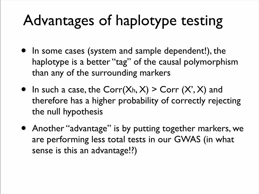
Advantages of haplotype testing

• In some cases (system and sample dependent!), the haplotype is a better “tag” of the causal polymorphism than any of the surrounding markers

• In such a case, the Corr(Xh, X) > Corr (X’, X) and therefore has a higher probability of correctly rejecting the null hypothesis

• Another “advantage” is by putting together markers, we are performing less total tests in our GWAS (in what sense is this an advantage!?)

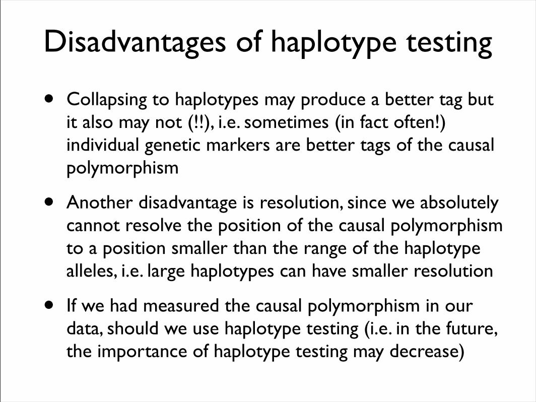
Disadvantages of haplotype testing

• Collapsing to haplotypes may produce a better tag but it also may not (!!), i.e. sometimes (in fact often!) individual genetic markers are better tags of the causal polymorphism

• Another disadvantage is resolution, since we absolutely cannot resolve the position of the causal polymorphism to a position smaller than the range of the haplotype alleles, i.e. large haplotypes can have smaller resolution

• If we had measured the causal polymorphism in our data, should we use haplotype testing (i.e. in the future, the importance of haplotype testing may decrease)

Should I apply haplotype testing in my GWAS?

• Yes! but apply both an individual marker testing approach (always!) as well as a haplotype test (optional)

• The reason is that we never know the true answer in our GWAS (as with any statistical analysis!) so it doesn’t hurt us to explore our dataset with as many techniques as we want to apply

• In fact, this will be a continuing theme of the class, i.e. keep analyzing GWAS with as many methods as you find useful

• However, since we never know the right answer for certain, if we get conflicting results, which one do we interpret as “correct”!?

Where do haplotypes come from?

• A deep discussion of the origin of haplotypes (remember: a fuzzy definition!) is another subject that is in the realm of population genetics and therefore we cannot discuss this in detail in this class (again: I encourage you to take a class on population genetics!)

• However, we can get an intuition about where haplotypes come from by remembering that the origin of new haplotype alleles are mutations and that new haplotype alleles can be produced by recombination

• In fact, these two processes also underlie the amount of LD in the population and therefore what blocks of alleles are inherited as a haplotype (and we therefore use them to define haplotypes using system specific criteria)

Defining haplotypes

• We could spend multiple lectures on how people define haplotypes for given systems and the algorithms used for this purpose (so we will just briefly mention the main concepts here)

• To define haplotypes, we need to “phase” measured genotype markers, decide on the number of genotype markers to put together into a haplotype block, and decide how many haplotype alleles to consider

• Remember: there are no universal rules for doing this (system dependent!)

Phasing haplotypes

• To get a sense of the phasing problem, consider a case where we have two markers that are right next to each other on a chromosome and we know we want to put them together in a haplotype block

• Say one marker is (A,T) and the other marker is (G,C) and we are considering a diploid individual who is a heterozygote for both of these markers, which of the marker alleles are physically linked in this individual?

• Figuring this out for individuals in a sample is the phasing problem and there are many algorithms for accomplishing this goal (note that in the future, technology may make this a non-issue...)

Deciding on how many genotypes to include in a haplotype block• Again, while there is no set rule, how we decide on

genotypes to include in a haplotype block depends on LD

• The general rule: if we have a set of markers in high LD with each other but low LD with other markers, we use this as a guide for defining the haplotype block

vbay

post

erio

rpro

babi

lity

cM/M

b

T1D hit region, chromosome 1( rs613232 )

cMfro

mhi

t�

log 1

0(P)

CDhit region, chromosome 10( rs10995271 )

0

5

10

15

0

0.2

0.4

0.6

0.8

1ZNF365ADOEGR2

genes

03060

012

64.2 64.3 64.4 64.5 64.6 64.7

**

0

5

10

15

0

0.2

0.4

0.6

0.8

1RCOR3TRAF5C1orf97RD3SLC30A1NEK2LPGAT1

genes

03060

012

211.5 211.6 211.7 211.8 211.9 212.0

**

Single marker testConditional testVBAYLassoAdaptive Lasso2D-MCPLOGNEGIndependent hitNon7independent hit

0

5

10

15

0

0.2

0.4

0.6

0.8

1LPHN2

genes

03060

012

81.5 82.0 82.5 83.0

Deciding on how many haplotype alleles to consider

• Again, there are no set rules for how many haplotype alleles to define, but in general, we define a set where the frequency in a population is above some MAF threshold (which depends on the system)

• With a MAF cutoff of say 0.05, this generally limits us to 2-5 haplotype alleles (e.g. in humans!)

• There are however cases where we might want to consider rarer haplotypes (what are some of these?)

Haplotype GWAS wrap-up

• Haplotypes are a physical and sampling consequence of how genetic systems work (just like LD!)

• Definitions of haplotype blocks and haplotype alleles depend on the system and context (fuzzy definition)

• Regardless of how we define them, once we have haplotype alleles, we can use them as we would genetic markers in our GWAS analysis framework

• While optional, it is never a bad idea to perform a haplotype analysis of your GWAS in addition to your single marker analysis (ALWAYS do a single marker analysis)

That’s it for today

• Next lecture: we will discuss covariates, including one of the most important (population structure)!

• We will also discuss a “minimum checklist” that you should perform in your GWAS analysis (!!)