42
ISQS 3344 Introduction to Production and Operations Management Spring 2014 Quantitative Review I
| Date post: | 22-Dec-2015 |
| Category: |
Documents |
| Upload: | jenna-gotts |
| View: | 214 times |
| Download: | 0 times |

ISQS 3344 Introduction to Production and
Operations Management
Spring 2014
Quantitative Review I

SUPPLEMENT 7Capacity and Constraint Management
(Break-Even Analysis)

Portland Radio Company (PRC) is trying to decide whether or not to introduce a new model. If they introduce it, there will be additional fixed costs of $400,000 per year. The variable costs have been estimated to be $30 per radio. If PRC sells the new radio model for $40 per radio, how many must they sell to break even?
VCSP
FQ
unitsQ 000,4030$40$
000,400$
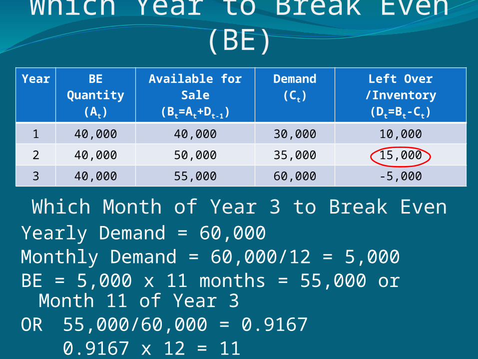
Which Year to Break Even (BE)Year BE
Quantity(At)
Available for Sale
(Bt=At+Dt-1)
Demand(Ct)
Left Over /Inventory(Dt=Bt-Ct)
1 40,000 40,000 30,000 10,000
2 40,000 50,000 35,000 15,000
3 40,000 55,000 60,000 -5,000
Which Month of Year 3 to Break EvenYearly Demand = 60,000Monthly Demand = 60,000/12 = 5,000BE = 5,000 x 11 months = 55,000 or Month
11 of Year 3OR 55,000/60,000 = 0.9167
0.9167 x 12 = 11

CHAPTER 1Operations and Productivity
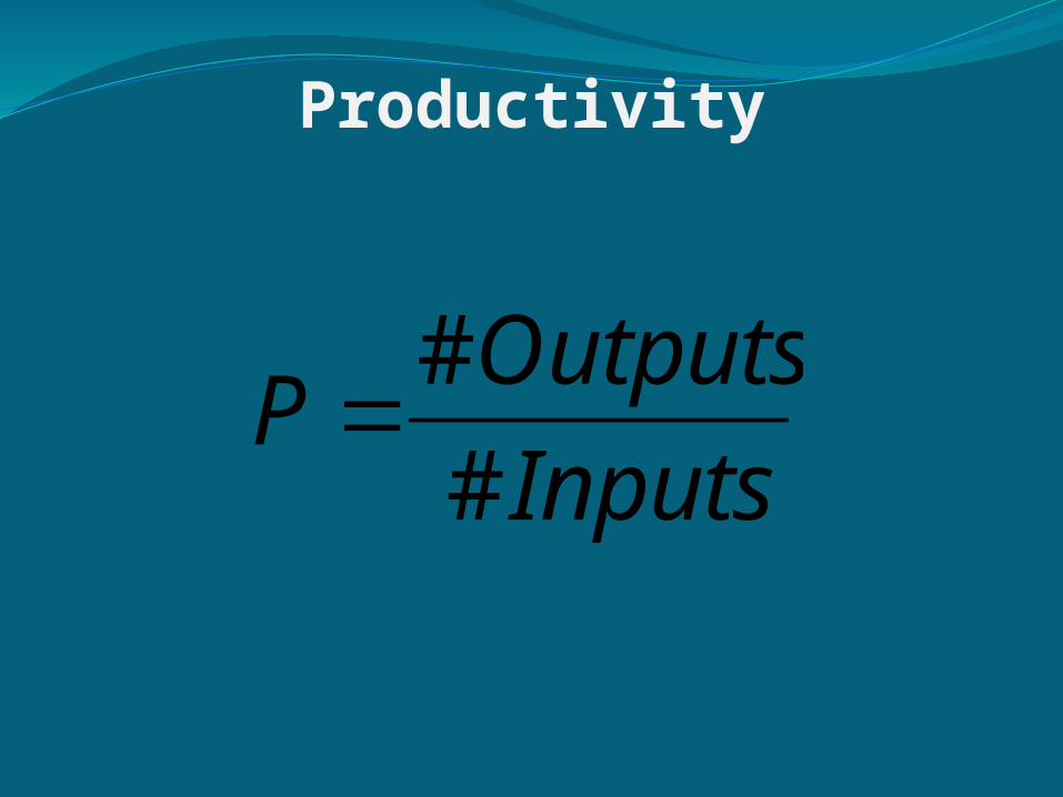
Productivity
Inputs
OutputsP
#
#

Labor Productivity
hourtablehours
tables
Inputs
OutputsP /1
24
24
Three workers paint twenty-four tables in eight hours
Inputs: 24 hours of labor (3 workers x 8 hours)Outputs: 24 painted tables
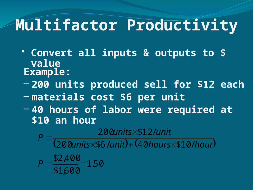
Multifactor Productivity
• Convert all inputs & outputs to $ value
50.1600,1$
400,2$
/10$40/6$200
/12$200
P
hourhoursunitunits
unitunitsP
Example:– 200 units produced sell for $12 each– materials cost $6 per unit– 40 hours of labor were required at
$10 an hour
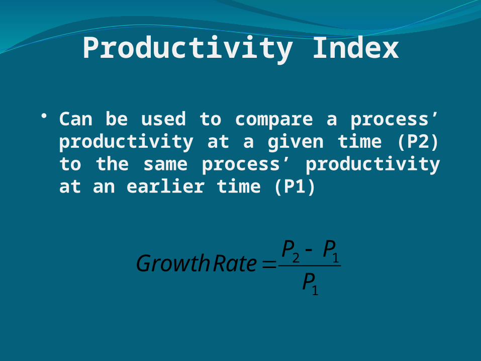
Productivity Index
• Can be used to compare a process’ productivity at a given time (P2) to the same process’ productivity at an earlier time (P1)
1
12
P
PPRateGrowth

Productivity Growth RateExample:– Last week, a company produced 150 units
using 200 hours of labor.– This week, the same company produced 170
units using 240 hours of labor.
hourunitshours
unitsP
hourunitshours
unitsP
/71.0240
170
/75.0200
150
2
1
rategrowthnegativeaor
P
PPRateGrowth
%5
05.075.0
75.071.0
1
12

If inputs increase by 25% and outputs decrease by 10%, what is the percentage change in productivity? Assume P1 = 1/1.
decreaseorChange
Change
P
P
%2828.%1
172.0%
72.025.1
90.0
11
1
2
1

Production increased to 75 from 65 pieces per day. Defective items have dropped from 12 to 5 pieces per day. Production facility operates eight hours per day. Seven people work daily in the plant. What is the change in productivity?Period 1 Output = 65 Defects = 12 Net Output = 53Period 2 Output = 75 Defects = 5 Net Output = 70Period 1 Input = 8 hours x 7 workers = 56Period 2 Input = 8 hours x 7 workers = 56
P1 = 53/56 = 0.95P2 = 70/56 = 1.25Change = (1.25-0.95)/0.95 = 0.32

CHAPTER 2Revenue Management Systems
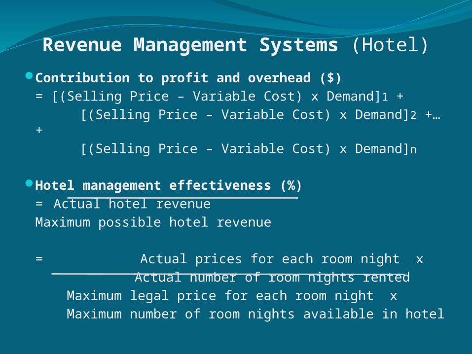
Revenue Management Systems (Hotel)Contribution to profit and overhead ($)
= [(Selling Price – Variable Cost) x Demand]1 + [(Selling Price – Variable Cost) x Demand]2 +… + [(Selling Price – Variable Cost) x Demand]n
Hotel management effectiveness (%)= Actual hotel revenueMaximum possible hotel revenue
= Actual prices for each room night x Actual number of room nights rented Maximum legal price for each room night x Maximum number of room nights available in hotel

Hotel ManagementCharacteristic/Variable Business
Hotel Customers Convention Association
Hotel Customers Customers for this day (Demand)
400 room nights rented
800 room nights rented
Average price/room night (Selling Price) $200 $120
Variable cost/room night (Variable cost)
$50 $50
Maximum price/room night $250 $150
Maximum number rooms available for sale this day
500 room nights available
900 room nights available

Hotel ManagementContribution to profit and overhead ($)
= [(Selling Price – Variable Cost) x Demand]= [($200 - $50) x 400] + [($120 - $50) x 800]= ($150 x 400) + ($70 x 800) = $116,000
Hotel management effectiveness (%)= Actual prices for each room night x Actual number of room nights rented
Maximum legal price for each room night x Maximum number of room nights available in hotel= ($200 x 400 rooms) + ($120 x 800 rooms) ($250 x 500 rooms) + ($150 x 900 rooms)= ($80,000 + $96,000) / ($125,000 + $135,000) = 67.69%
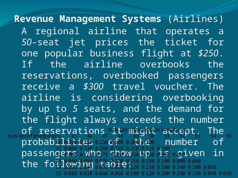
Revenue Management Systems (Airlines)A regional airline that operates a 50-seat jet prices the ticket for one popular business flight at $250. If the airline overbooks the reservations, overbooked passengers receive a $300 travel voucher. The airline is considering overbooking by up to 5 seats, and the demand for the flight always exceeds the number of reservations it might accept. The probabilities of the number of passengers who show up is given in the following table:
Number of reservations 45 46 47 48 49 50 51 52 53 54 5550 0.100 0.150 0.150 0.200 0.300 0.10051 0.080 0.130 0.180 0.150 0.250 0.110 0.10052 0.060 0.125 0.175 0.200 0.250 0.100 0.050 0.04053 0.040 0.050 0.070 0.200 0.250 0.150 0.100 0.080 0.06054 0.020 0.040 0.050 0.090 0.120 0.210 0.180 0.140 0.100 0.05055 0.010 0.030 0.040 0.060 0.100 0.120 0.200 0.180 0.150 0.090 0.020
Number of passengers showing up

Overbooking Strategies and AnalysisNumber of reservations 45 46 47 48 49 50 51 52 53 54 55
50 0.100 0.150 0.150 0.200 0.300 0.10051 0.080 0.130 0.180 0.150 0.250 0.110 0.10052 0.060 0.125 0.175 0.200 0.250 0.100 0.050 0.04053 0.040 0.050 0.070 0.200 0.250 0.150 0.100 0.080 0.06054 0.020 0.040 0.050 0.090 0.120 0.210 0.180 0.140 0.100 0.05055 0.010 0.030 0.040 0.060 0.100 0.120 0.200 0.180 0.150 0.090 0.020
Number of passengers showing up
Expected revenue for 50 reservations = $250 x (45*.1 + 46*.15 + 47*.15 + 48*.2 + 49*.3 + 50*.1) = $11,937.50Expected re venue for 51 reservations = [$250 x (45*.08 + 46*.13 + 47*.18 + 48*.15 + 49*.25 + 50*.11)] – ($300 x .1) = 10,717.50Expected re venue for 52 reservations = [$250 x (45*.06 + 46*.125 + 47*.175 + 48*.2 + 49*.25 + 50*.1)] – [$300 x (.05+.04)] = $10,854.25Expected re venue for 53 reservations = [$250 x (45*.04 + 46*.05 + 47*.07 + 48*.2 + 49*.25 + 50*.15)] – [$300 x (.1+.08+.06)] = $9,113Expected revenue for 54 reservations = $6,306.50Expected revenue for 55 reservations = $4,180.50

CHAPTER 4Forecasting
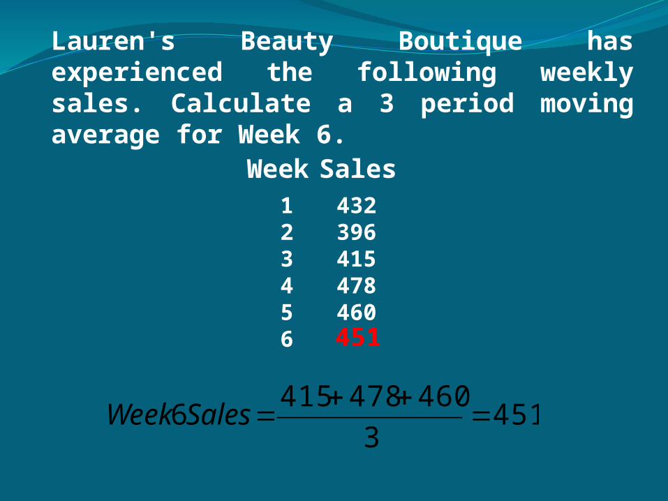
Lauren's Beauty Boutique has experienced the following weekly sales. Calculate a 3 period moving average for Week 6.
Week Sales123456
432396415478460451
4513
4604784156
SalesWeek
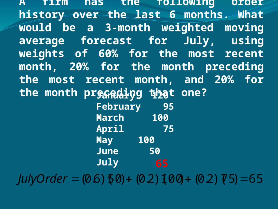
A firm has the following order history over the last 6 months. What would be a 3-month weighted moving average forecast for July, using weights of 60% for the most recent month, 20% for the month preceding the most recent month, and 20% for the month preceding that one?
January 120February 95March 100April 75May 100June 50July
65)75)(2.0()100)(2.0()50)(6.0( JulyOrder65

Exponential Smoothing
– Last period’s actual value (At)– Last period’s forecast (Ft)– Select value of smoothing coefficient, between 0
and 1.0
ttt FAF 11

Summary of Single Exponential Smoothing Milk-Sales Forecasts with α = 0.2
F2 = .2(172) + .8(172) =172
F3 = .2(217) + .8(172) = 181
F4 = .2(190) + .8(181) = 182.8
F5 = .2(233) + .8(182.8) = 192.84
F6 = .2(179) + .8(192.84) = 190.07
F7……….
You start with past data and calculate forecasts working forward.
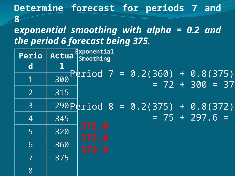
Determine forecast for periods 7 and 8exponential smoothing with alpha = 0.2 and the period 6 forecast being 375.
Period Actual
1 300
2 315
3 290
4 345
5 320
6 360
7 375
8 372.6372.0
ExponentialSmoothing
Period 7 = 0.2(360) + 0.8(375) = 72 + 300 = 372.0
Period 8 = 0.2(375) + 0.8(372) = 75 + 297.6 = 372.6
375.0

Quarterly ForecastingExpected total demand in 2012 is 3,000 units. Given the historical sales figures below, derive a forecast for each quarter in 2012.
2009250500700900
0.430.851.191.53
2010270530800970
0.420.821.251.51
20113106008501000
0.450.871.231.45
Q1Q2Q3Q4
0.430.851.221.50
2350 2570 2760Total
Quarter 587.5 642.5 690
20123246369171123
3000
750
250/587.5
(1.53+1.51+1.45)/3
750 x 0.43

The Regression Equation orTrend Forecast
bXayTx
xT = trend forecast or y variable
a = estimate of Y-axis intercept where X = 0
b = estimate of slope of the demand line
X = period number or independent variable
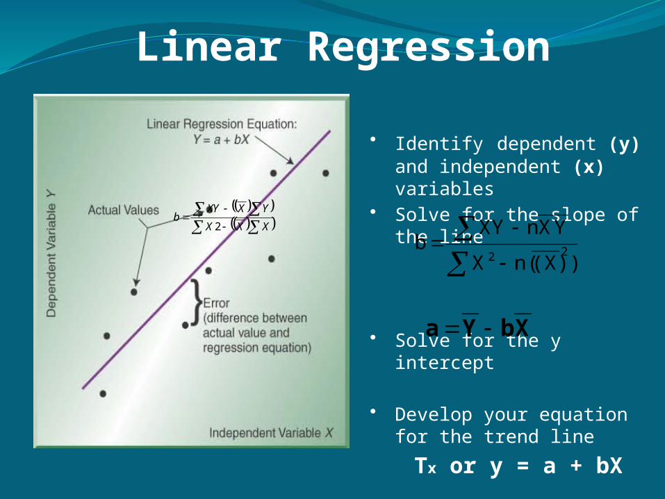
Linear Regression
XXX
YXXYb
2
• Identify dependent (y) and independent (x) variables
• Solve for the slope of the line
• Solve for the y intercept
• Develop your equation for the trend line
Tx or y = a + bX
XbYa
)(X)n(X
YXnXYb 22
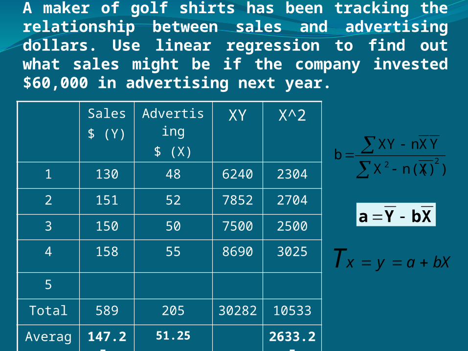
A maker of golf shirts has been tracking the relationship between sales and advertising dollars. Use linear regression to find out what sales might be if the company invested $60,000 in advertising next year.
)X)n((X
YXnXYb 22
Sales$ (Y)
Advertising$ (X)
XY X^2
1 130 48 6240 2304
2 151 52 7852 2704
3 150 50 7500 2500
4 158 55 8690 3025
5
Total 589 205 30282 10533
Average 147.25 51.25 2633.25
XbYa
bXayxT

Y = a + bXY = -36.17 + 3.579XY = -36.17 + 3.579(60)Y = 178.57 or $178,570 in sales
)X)n((X
YXnXYb 22
XbYa
a = 147.25-3.579(51.25) = -36.17
XbYa
579.375.26
75.95
)25.51(410533
)25.147)(25.51(430282b
2

Tracking Forecast Error Over Time
• Mean Absolute Deviation (MAD)– A good measure of the actual error in
a forecast
• Tracking Signal (TS)
– Exposes bias (positive or negative)Positive TS = under-forecastingNegative TS = over-forecasting
MAD
TS forecast - actual
n
1=iii FA
n
1=MAD

Mean Absolute Deviation• MAD sums only absolute values errors, both
positive and negative errors add to the sum and the average size of the error (whether positive or negative) is determined.
n = number of periods of dataF = forecast of demand in period iA = actual demand in period i
n
1=iii FA
n
1=MAD
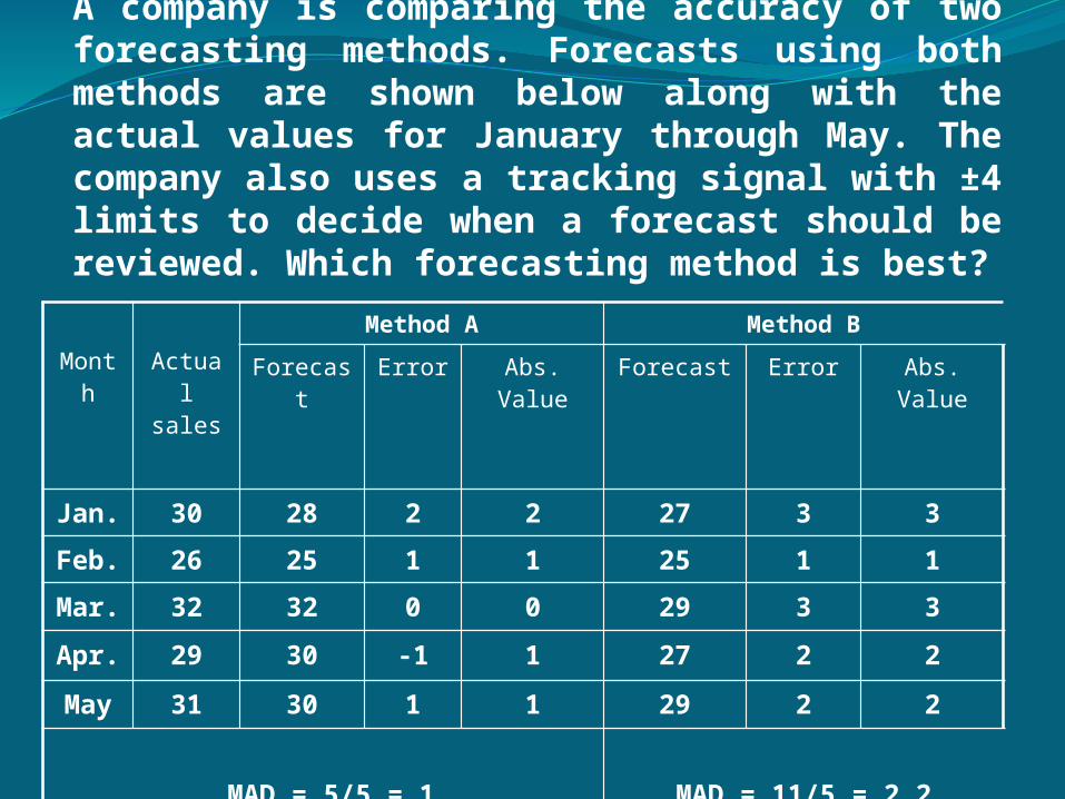
A company is comparing the accuracy of two forecasting methods. Forecasts using both methods are shown below along with the actual values for January through May. The company also uses a tracking signal with ±4 limits to decide when a forecast should be reviewed. Which forecasting method is best?
Month Actual sales
Method A Method B
Forecast Error Abs. Value Forecast Error Abs. Value
Jan. 30 28 2 2 27 3 3
Feb. 26 25 1 1 25 1 1
Mar. 32 32 0 0 29 3 3
Apr. 29 30 -1 1 27 2 2
May 31 30 1 1 29 2 2
MAD = 5/5 = 1TS = 3/1 = 3
MAD = 11/5 = 2.2TS = 11/2.2 = 5

Supplement 7Capacity and Constraint
Management
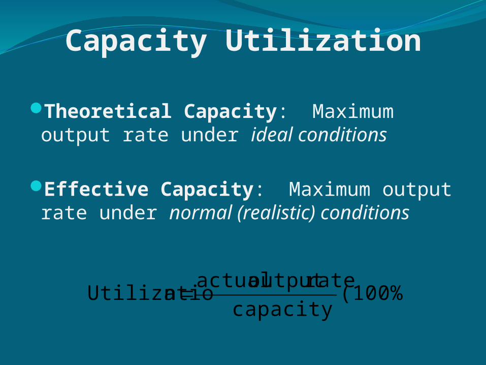
Capacity Utilization
Theoretical Capacity: Maximum output rate under ideal conditions
Effective Capacity: Maximum output rate under normal (realistic) conditions
(100%)capacity
rateoutput actualn Utilizatio
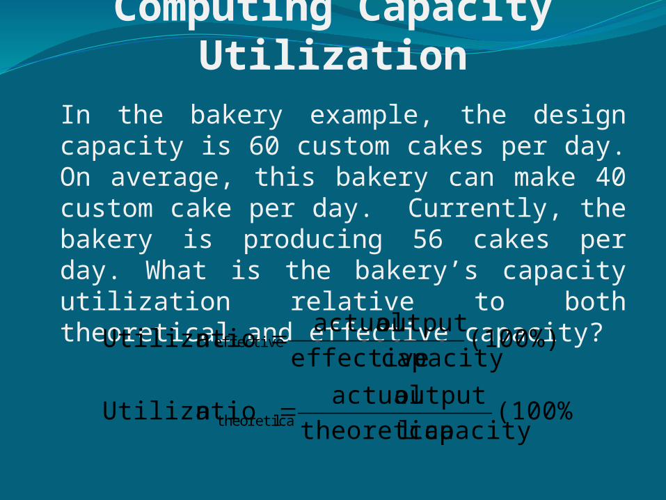
Computing Capacity Utilization
(100%)capacity ltheoretica
output actualn Utilizatio
(100%)capacity effective
output actualn Utilizatio
ltheoretica
effective
In the bakery example, the design capacity is 60 custom cakes per day. On average, this bakery can make 40 custom cake per day. Currently, the bakery is producing 56 cakes per day. What is the bakery’s capacity utilization relative to both theoretical and effective capacity?

Computing Capacity UtilizationIn the bakery example, the design capacity is 60 custom cakes per day. On average, this bakery can make 40 custom cake per day. Currently, the bakery is producing 56 cakes per day. What is the bakery’s capacity utilization relative to both theoretical and effective capacity?
93%(100%)60
56(100%)
capacity ltheoretica
output actualn Utilizatio
140%(100%)40
56(100%)
capacity effective
output actualn Utilizatio
ltheoretica
effective

A clinic has been set up to give flu shots to the elderly in a large city. The theoretical capacity is 80 seniors per hour, and the effective capacity is 55 seniors per hour. Yesterday the clinic was open for ten hours and gave flu shots to 350 seniors.
What is the effective utilization?What is the theoretical utilization?
%75.34(100%)80
350/10(100%)
capacity ltheoretica
output actualn Utilizatio
%64.36(100%)55
350/10(100%)
capacity effective
output actualn Utilizatio
ltheoretica
effective

Decision Trees• Build from the present to the future:
– Distinguish between decisions (under your control) & chance events (out of your control, but can be estimated to a given probability)
• Solve from the future to the present:– Generate an expected value for
each decision point based on probable outcomes of subsequent events
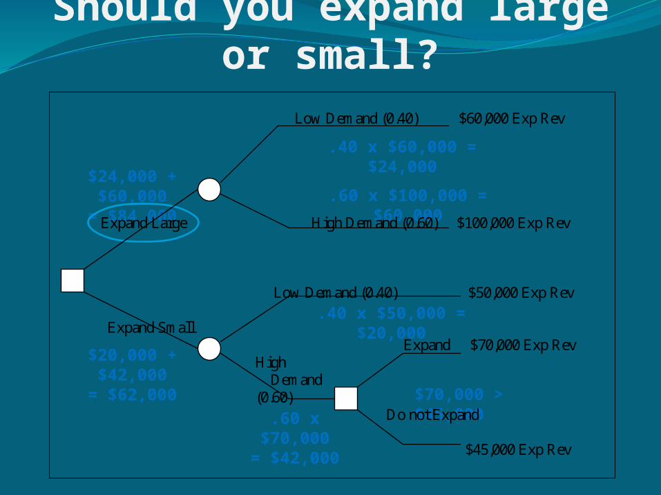
Should you expand large or small? Low Demand (0.40) $60,000 Exp Rev Expand Large High Demand (0.60) $100,000 Exp Rev Low Demand (0.40) $50,000 Exp Rev
Expand Small Expand $70,000 Exp Rev High Demand (0.60) Do not Expand $45,000 Exp Rev
$70,000 > $45,000.60 x
$70,000= $42,000
.40 x $50,000 = $20,000
$20,000 + $42,000
= $62,000
.40 x $60,000 = $24,000
.60 x $100,000 = $60,000
$24,000 + $60,000
= $84,000
Capacity AnalysisCapacity analysis determines the
throughput capacity of workstations in a system.
A bottleneck is a limiting factor or constraint.
A bottleneck has the lowest effective capacity in a system or takes the most time.
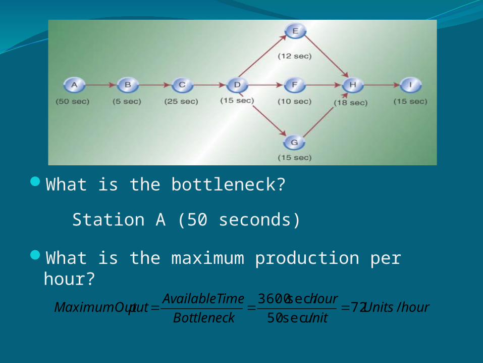
What is the bottleneck?
What is the maximum production per hour?
Station A (50 seconds)
hourUnitsunit
hour
Bottleneck
imeAvailableTputMaximumOut /72
sec/50
sec/3600

That’s all, folks!
Thanks for today!


