Quantitative unique continuation from

measurable set for some PDE�s�

Kim Dang PHUNGUniversité d�Orléans, Laboratoire MAPMO, CNRS UMR 7349,

Fédération Denis Poisson, FR CNRS 2964,Bâtiment de Mathématiques,

B.P. 6759, 45067 Orléans Cedex 2, FranceE-mail: kim_dang_phung@yahoo.fr

Abstract

In this note, we provide quantitative unique continuation results froma measurable set with positive measure for di¤erent PDE�s like heat equa-tion, wave equation and Schrödinger equation in a bounded domain withhomogeneous Dirichlet boundary condition. We extend the well-knownresults for a non-empty open subset to a measurable subset with positivemeasure. Our motivation comes from the fact that many recent resultsin the �eld of optimization and control theory for PDE�s require to studydistributed system with an acting on a positive measurable set insteadthat on a non-empty open subset.

Contents

1 Preliminary result on Laplace�s equation 2

2 Heat equation 3

3 Schrödinger equation 3

4 Wave equation 4

5 Proof for the Heat equation 55.1 Logarithmic estimate (proof of i)) iii)) . . . . . . . . . . . . . . 55.2 Observability estimate (proof of ii)) i)) . . . . . . . . . . . . . 65.3 Hölder estimate . . . . . . . . . . . . . . . . . . . . . . . . . . . . 9

6 Proof for the Schrödinger equation 9

�This note was done when the author visited Yangtze Center of Mathematics, SichuanUniversity, Chengdu, China, (August 1-30, 2012).

1

7 Proof for the wave equation 147.1 The FBI approach . . . . . . . . . . . . . . . . . . . . . . . . . . 147.2 The resolvent approach . . . . . . . . . . . . . . . . . . . . . . . 19

Our �rst result concerns the heat equation. Three type of quantitativeunique continuation are given. (i) is a re�ned observability estimate. (ii) isan Hölder type of estimate. (iii) is a logarithmic type of estimate.

The second result treats the Schrödinger equation in a bounded domain .It quanti�es the fact that, for smooth and non-identically zero initial data, thesolution can not vanish on E�(0; T ) where E � is a measurable set of positivemeasure.

The third result deals with the wave equation. In dimension higher thanone, we can not expect an observability estimate when the observation is madeon an arbitrary subset of positive measure (see [Ru], [BLR]). The observabilityconstant or the time of controllability may depend on the frequency quantity� (u0; u1) (which depends on the initial data (u0; u1)). Further, notice that ourresult quanti�es the unique continuation result of Dafermos (see [H]).

We hope that this result will prove useful in control theory.

1 Preliminary result on Laplace�s equation

Let D � RN+1, N � 1, be a connected bounded open set with boundary @D.Let � be a non-empty Lipschitz open part of @D. We consider the Laplacian inD, with a homogeneous Dirichlet boundary condition on � � @:8<: �yv = 0 in D ,

v = 0 on � ,v = v (y) 2 H2 (D) .

(D.1)

Theorem 1 .- Let E � D be a measurable set of positive measure.Then, for any D1 � D such that @D1\@D b � and D1 n(� \ @D1) � D, thereexist C > 0 and � 2 (0; 1) such that for any v solution of (D.1), we have

kvkL2(D1)� C kvk�L1(E) kvk

1��L2(D) .

Many works deals with similar estimate. We refer to [V], [MV], [AE],[AEWZ], [R], e.g.

2

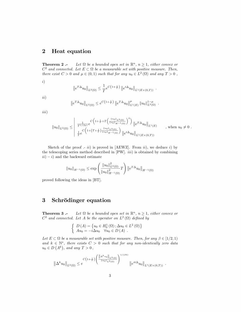
2 Heat equation

Theorem 2 .- Let be a bounded open set in Rn, n � 1, either convex orC2 and connected. Let E � be a measurable set with positive measure. Then,there exist C > 0 and � 2 (0; 1) such that for any u0 2 L2 () and any T > 0 ,

i) eT�u0 L2() � 1

TeC(1+

1T ) et�u0 L1(E�(0;T )) .

ii) eT�u0 L2() � eC(1+ 1T ) eT�u0 �L1(E) ku0k1��L2() .

iii)

ku0kL2() �

��������1

T 1=(2�)eC

�1+ 1

T +T

� ku0kL2()ku0kH�1()

�2� eT�u0 L1(E)1T e

C

�1+(T+ 1

T )ku0kL2()ku0kH�1()

� et�u0 L1(E�(0;T )), when u0 6= 0 .

Sketch of the proof .- ii) is proved in [AEWZ]. From ii), we deduce i) bythe telescoping series method described in [PW]. iii) is obtained by combiningii)� i) and the backward estimate

ku0kH�1() � exp ku0k2L2()ku0k2H�1()

T

! eT�u0 H�1()

proved following the ideas in [BT].

3 Schrödinger equation

Theorem 3 .- Let be a bounded open set in Rn, n � 1, either convex orC2 and connected. Let A be the operator on L2 () de�ned by�

D (A) =�u0 2 H1

0 () ;�u0 2 L2 ()

Au0 = �i�u0 8u0 2 D (A) .

Let E � be a measurable set with positive measure. Then, for any � 2 [1=2; 1)and k 2 N�, there exists C > 0 such that for any non-identically zero datau0 2 D

�Ak�, and any T > 0 ,

�ku0 L2() � eC(1+ 1T )

0@k�ku0kL2()ku0kL2()

1A1=(�k) eit�u0 L1(E�(0;T )) .3

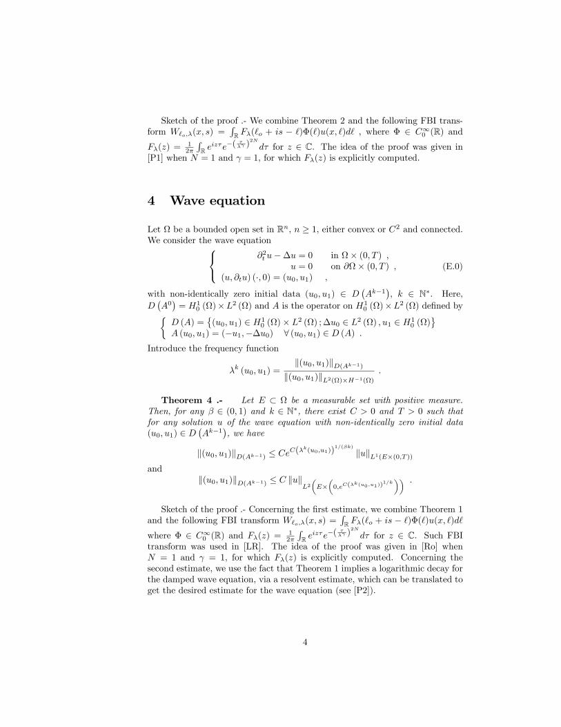
Sketch of the proof .- We combine Theorem 2 and the following FBI trans-form W`o;�(x; s) =

RR F�(`o + is � `)�(`)u(x; `)d` , where � 2 C10 (R) and

F�(z) =12�

RR e

iz�e�(�� )

2N

d� for z 2 C. The idea of the proof was given in[P1] when N = 1 and = 1, for which F�(z) is explicitly computed.

4 Wave equation

Let be a bounded open set in Rn, n � 1, either convex or C2 and connected.We consider the wave equation8<: @2t u��u = 0 in � (0; T ) ,

u = 0 on @� (0; T ) ,(u; @tu) (�; 0) = (u0; u1) ,

(E.0)

with non-identically zero initial data (u0; u1) 2 D�Ak�1

�, k 2 N�. Here,

D�A0�= H1

0 ()�L2 () and A is the operator on H10 ()�L2 () de�ned by�

D (A) =�(u0; u1) 2 H1

0 ()� L2 () ;�u0 2 L2 () ; u1 2 H10 ()

A (u0; u1) = (�u1;��u0) 8 (u0; u1) 2 D (A) .

Introduce the frequency function

�k (u0; u1) =k(u0; u1)kD(Ak�1)

k(u0; u1)kL2()�H�1()

.

Theorem 4 .- Let E � be a measurable set with positive measure.Then, for any � 2 (0; 1) and k 2 N�, there exist C > 0 and T > 0 such thatfor any solution u of the wave equation with non-identically zero initial data(u0; u1) 2 D

�Ak�1

�, we have

k(u0; u1)kD(Ak�1) � CeC(�k(u0;u1))

1=(�k)

kukL1(E�(0;T ))and

k(u0; u1)kD(Ak�1) � C kukL2�E��0;eC(�

k(u0;u1))1=k�� .

Sketch of the proof .- Concerning the �rst estimate, we combine Theorem 1and the following FBI transform W`o;�(x; s) =

RR F�(`o + is � `)�(`)u(x; `)d`

where � 2 C10 (R) and F�(z) = 12�

RR e

iz�e�(�� )

2N

d� for z 2 C. Such FBItransform was used in [LR]. The idea of the proof was given in [Ro] whenN = 1 and = 1, for which F�(z) is explicitly computed. Concerning thesecond estimate, we use the fact that Theorem 1 implies a logarithmic decay forthe damped wave equation, via a resolvent estimate, which can be translated toget the desired estimate for the wave equation (see [P2]).

4

5 Proof for the Heat equation

5.1 Logarithmic estimate (proof of i)) iii))

We look for an estimate of the form

ku (�; 0)k2H�1() � constant ku (�; T )k2L2() ,

where u solves the heat equation and T > 0. This is a backward estimate forthe heat equation. To do this, we apply the ideas in [BT] : Let us consider foralmost all t 2 [0; T ] such that u (x; t) 6= 0 the following quantity :

(t) =ku (�; t)k2L2()ku (�; t)k2H�1()

.

We �rst prove thatd

dt(t) � 0 .

Indeed we have the two following energy equalities:

1

2

d

dtku (�; t)k2L2() + ku (�; t)k

2H10 ()

= 0 ,

1

2

d

dtku (�; t)k2H�1() + ku (�; t)k

2L2() = 0 .

Then we get

d

dt(t) =

2

kuk4H�1()

��kuk2H1

0 ()kuk2H�1() + kuk

4L2()

�.

By Cauchy-Schwarz, we get the desired inequality. Consequently, we obtain forall t 2 (0; T ),

(t) � (0) .Secondly, remark that

0 = 12ddt ku (�; t)k

2H�1() +(t) ku (�; t)k

2H�1()

� 12ddt ku (�; t)k

2H�1() +(0) ku (�; t)k

2H�1() .

Consequently, integrating on (0; T ), we get the desired estimate :

ku (�; 0)kH�1() � exp ( (0)T ) ku (�; T )kH�1() .

Now, we apply eT�u0 L2() � eC(1+ 1

T ) eT�u0 �L1(E) ku0k1��L2() to get

ku (�; 0)kH�1() � exp ( (0)T ) eC(1+ 1

T ) eT�u0 �L1(E) ku0k(1��)L2() .

5

That is

ku0k�L2() �p(0) exp ( (0)T ) eC(1+

1T ) eT�u0 �L1(E) .

ku0kL2() ��1pTeC(1+

1T +(0)T)

�1=� eT�u0 L1(E) .Now we will prove the second estimate. Let us denote �1 > 0 a constant suchthat

�1 � (0) .Now, we choose

L = T

s�1(0)

� T ,

and recall that the solution u of the heat equation satis�es if u (x; t) 6= 0 foralmost all t 2 [0; T ] :

ku (�; 0)kH�1() � exp�p

�1(0)T� u

�; T

s�1(0)

! L2()

.

Now, we apply eL�u0 L2() � 1

LeC(1+ 1

L ) eit�u0 L1(E�(0;L)) to get

ku (�; 0)kH�1() �exp

�p�1(0)T

�Tq

�1(0)

eC

0@1+ 1

T

r�1(0)

1A et�u0 L1�E��0;Tq

�1(0)

�� .

Then,

ku (�; 0)kH�1() �p(0)

TeC�1+p(0)(T+ 1

T )� et�u0 L1(E�(0;T )) .

Thus,

ku0kL2() �1

TeC

�1+(T+ 1

T )ku0kL2()ku0kH�1()

� et�u0 L1(E�(0;T )) , when u0 6= 0 .

5.2 Observability estimate (proof of ii)) i))

Let ` 2 [0; T ) and `1 2 (`; T ]. Let z > 1. Introduce the decreasing sequencef`mgm�1, which converges to ` given by

`m+1 = `+1

zm(`1 � `) .

6

Then

`m � `m+1 =1

zm(z � 1) (`1 � `) > 0 .

We start with the following interpolation estimate. For any 0 � t1 < t2 � T ,

ku (�; t2)kL2() �C1" e

C2t2�t1 ku (�; t2)kL1(E) + " ku (�; t1)kL2() 8" > 0 .

Let 0 < `m+2 < `m+1 � t < `m < T . We get

ku (�; t)kL2() �C1" e

C2t�`m+2 ku (�; t)kL1(E) + " ku (�; `m+2)kL2() 8" > 0 .

Recall thatku (�; `m)kL2() � ku (�; t)kL2() .

Therefore,

ku (�; `m)kL2() �C1" e

C2t�`m+2 ku (�; t)kL1(E) + " ku (�; `m+2)kL2() 8" > 0 .

Integrating it over t 2 (`m+1; `m), it gives

(`m � `m+1) ku (�; `m)kL2() � C1" e

C2`m+1�`m+2

R `m`m+1

ku (�; t)kL1(E) dt+" (`m � `m+1) ku (�; `m+2)kL2() 8" > 0 .

That is

ku (�; `m)kL2() �h

1`1�`

zm

z�1

iC1" e

C2h

1`1�`

zm+1

z�1

i R `m`m+1

ku (�; t)kL1(E) dt+" ku (�; `m+2)kL2() 8" > 0 .

Then

ku (�; `m)kL2() � 1"

1zC1C2e2C2

h1

`1�`zm+1

z�1

i R `m`m+1

ku (�; t)kL1(E) dt+" ku (�; `m+2)kL2() 8" > 0 .

Take d = 2C2h

1`1�`

1z(z�1)

i. It gives

" e�dzm+2 ku (�; `m)kL2() � "1+ e�dz

m+2 ku (�; `m+2)kL2()� 1

zC1C2

R `m`m+1

ku (�; t)kL1(E) dt 8" > 0 .

Take " = e�dzm+2

, then

e�( +1)dzm+2 ku (�; `m)kL2() � e�(2+ )dz

m+2 ku (�; `m+2)kL2()� 1

zC1C2

R `m`m+1

ku (�; t)kL2(E) dt .

7

Take z =q

+2 +1 , then

e�(2+ )dzm ku (�; `m)kL2() � e�(2+ )dz

m+2 ku (�; `m+2)kL2()�q

+1 +2

C1C2

R `m`m+1

ku (�; t)kL1(E) dt .

Change m to 2m0 and sum the above from m0 = 1 to in�nity give the desiredresult For simplicity, we only need to take ` = 0 and `1 = T , and get

e�(2+ )2C2

24 1T

r +2 +1r

+2 +1

�1

35ku (�; T )kL2()

� e�(2+ )dz2 ku (�; `2)kL2()�P

m0�1

�e�(2+ )dz

2m0ku (�; `2m0)kL2() � e�(2+ )dz

2m0+2 ku (�; `2m0+2)kL2()�

�P

m0�1

q +1 +2

C1C2

R `2m0`2m0+1

ku (�; t)kL1(E) dt

�q

+1 +2

C1C2

R `20ku (�; t)kL1(E) dt .

Finally,

ku (�; T )kL2() �r + 1

+ 2

C1C2e2C2

1T (2+ )

p +2[

p +2+

p +1]

Z T

0

ku (�; t)kL1(E) dt .

In particular,

ku (�; 1)kL2() �r + 1

+ 2

C1C2e2C2(2+ )

p +2[

p +2+

p +1]

Z 1

0

ku (�; t)kL1(E) dt

and

ku (�;m)kL2() �r + 1

+ 2

C1C2e2C2(2+ )

p +2[

p +2+

p +1]

Z m

m�1ku (�; t)kL1(E) dt

for any m � 1. Now, take T > 1 such that M < T �M + 1 for some M � 1,

T2 ku (�; T )kL2()

�M ku (�;M)kL2()�PM

m=1 ku (�;m)kL2()�q

+1 +2

C1C2e2C2(2+ )

p +2[

p +2+

p +1]PM

m=1

Rmm�1 ku (�; t)kL1(E) dt

�q

+1 +2

C1C2e2C2(2+ )

p +2[

p +2+

p +1] RM

0ku (�; t)kL1(E) dt

�q

+1 +2

C1C2e2C2(2+ )

p +2[

p +2+

p +1] R T

0ku (�; t)kL1(E) dt .

We conclude that for any T � 1,

ku (�; T )kL2() �1

T

r + 1

+ 2

C1C2e2C2

1T (2+ )

p +2[

p +2+

p +1]

Z T

0

ku (�; t)kL1(E) dt ,

8

and for any T > 1

ku (�; T )kL2() �2

T

r + 1

+ 2

C1C2e2C2(2+ )

p +2[

p +2+

p +1]

Z T

0

ku (�; t)kL1(E) dt .

Combining the case T � 1 and the case T > 1, we get the following observabilityestimate.

ku (�; T )kL2() �2

T

r + 1

+ 2

C1C2e4C2(1+

1T )(2+ )

2

Z T

0

ku (�; t)kL1(E) dt

for any T > 0.

5.3 Hölder estimate

This is Theorem 6 in [AEWZ].

6 Proof for the Schrödinger equation

Denote u (x; t) = eit�u0 (x). First, recall that with a standard energy method,we have that

8t 2 R ku0k2L2() =Z

ju (x; t)j2 dx , (E.1)

and

8j 2 N� �ju0 2L2() = Z

���@jt u (x; t)���2 dx. (E.2)

Next, let � 2 [1=2; 1), k 2 N�, and choose N 2 N� such that � + 12N � 1

and 2N > k. Put = 1 � 12N . For any � � 1, the function F�(z) =

12�

RR e

iz�e�(�� )

2N

d� is holomorphic in C, and there exists four positive con-stants Co, c0, c1 and c2 (independent on �) such that(

8z 2 C jF�(z)j � Co� ec0�jImzj1=

,jImzj � c2 jRezj ) jF�(z)j � Co� e�c1�jRezj

1=

,(E.3)

(see [LR]).

Now, let s; `o 2 R, we introduce the following Fourier-Bros-Iagolnitzer trans-formation in [LR]:

W`o;�(x; s) =

ZRF�(`o + is� `)�(`)u(x; `)d` , (E.4)

9

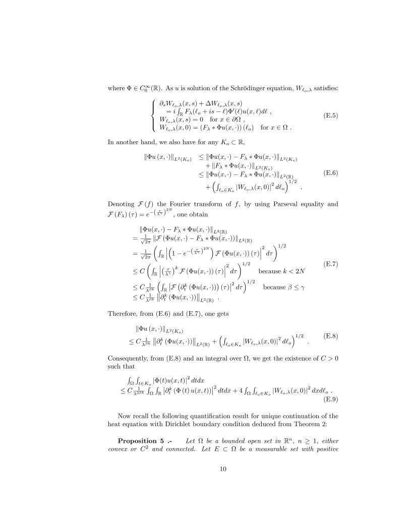
where � 2 C10 (R). As u is solution of the Schrödinger equation, W`o;� satis�es:8>><>>:@sW`o;�(x; s) + �W`o;�(x; s)= iRR F�(`o + is� `)�

0(`)u(x; `)d` ,W`o;�(x; s) = 0 for x 2 @ ,W`o;�(x; 0) = (F� � �u(x; �)) (`o) for x 2 .

(E.5)

In another hand, we also have for any Ko � R,

k�u (x; �)kL2(Ko)� k�u(x; �)� F� � �u(x; �)kL2(Ko)

+ kF� � �u(x; �)kL2(Ko)

� k�u(x; �)� F� � �u(x; �)kL2(R)+�R

`o2KojW`o;�(x; 0)j

2d`o

�1=2.

(E.6)

Denoting F (f) the Fourier transform of f , by using Parseval equality and

F (F�) (�) = e�(�� )

2N

, one obtain

k�u(x; �)� F� � �u(x; �)kL2(R)= 1p

2�kF (�u(x; �)� F� � �u(x; �))kL2(R)

= 1p2�

�RR

����1� e�( �� )

2N�F (�u(x; �)) (�)

���2 d��1=2� C

�RR

���� �� �k F (�u(x; �)) (�)���2 d��1=2 because k < 2N

� C 1��k

�RR

��F �@kt (�u(x; �))� (�)��2 d��1=2 because � � � C 1

��k

@kt (�u(x; �)) L2(R) .

(E.7)

Therefore, from (E.6) and (E.7), one gets

k�u (x; �)kL2(Ko)

� C 1��k

@kt (�u(x; �)) L2(R) + �R`o2KojW`o;�(x; 0)j

2d`o

�1=2.

(E.8)

Consequently, from (E.8) and an integral over , we get the existence of C > 0such thatR

Rt2Ko

j�(t)u(x; t)j2 dtdx� C 1

�2�k

R

RR

��@kt (� (t)u(x; t))��2 dtdx+ 4 R R`o2KojW`o;�(x; 0)j

2dxd`o .

(E.9)

Now recall the following quanti�cation result for unique continuation of theheat equation with Dirichlet boundary condition deduced from Theorem 2:

Proposition 5 .- Let be a bounded open set in Rn, n � 1, eitherconvex or C2 and connected. Let E � be a measurable set with positive

10

measure. Let " 2 (0; 1). Let f = f (x; s) 2 L2 (� (0; ")). Then for anyw = w (x; s) solution of8<: @sw +�w = f in � (0; ") ,

w = 0 on @� (0; ") ,w (�; ") 2 L2 () ,

we haveZ

jw (x; 0)j2 dx � CeC=""�Z "

0

ZE

jw (x; s)j dxds�2+

Z "

0

Z

jf (x; s)j2 dxds#,

for some C > 0 which only depends on and E.

Applying Proposition 5 to W`o;�, we getRjW`o;�(x; 0)j

2dx

� CeC="�R "0

REjW`o;� (x; s)j dxds

�2+CeC="

R "0

R

��i RR F�(`o + is� `)�0(`)u(x; `)d`��2 dxds . (E.10)

Next, we integrate over Ko and deduce thatR`o2Ko

RjW`o;�(x; 0)j

2dxd`o

� CeC="R`o2Ko

�R "0

REjW`o;� (x; s)j dxds

�2d`o

+CeC="R`o2Ko

R "0

R

��i RR F�(`o + is� `)�0(`)u(x; `)d`��2 dxdsd`o .(E.11)

ThereforeR

Rt2Ko

j�(t)u(x; t)j2 dtdx� C 1

�2�k

R

RR

��@kt (� (t)u(x; t)))��2 dtdx+4CeC="

R`o2Ko

�R "0

REjW`o;� (x; s)j dxds

�2d`o

+4CeC="R`o2Ko

R "0

R

��i RR F�(`o + is� `)�0(`)u(x; `)d`��2 dxdsd`o .(E.12)

Let T 2�0; 8c2

�. Let de�ne � 2 C10 (R) more precisely now: we choose

� 2 C10 ((0; T )), 0 � � � 1, � � 1 on�T4 ;

3T4

�such that sup

t2Rj�0 (t)j � 8

T .

Furthermore, let K =�0; T4

�[�3T4 ; T

�such that jKj = T

2 and supp(�0) = K.

Let Ko =�3T8 ;

5T8

�. In particular, jKoj = T

4 and dist(K;Ko) =T8 . Now,

we will choose " = c2T8 2 (0; 1) and `o 2 Ko. Consequently, for any ` 2 K,

j`0 � `j � T8 =

"c2� 1

c2jsj and it will imply from the second line of (E.3) that

8` 2 K jF�(`o + is� `)j � Co� e�c1�(T8 )

1=

. (E.13)

Till the end of the proof, C will denote a generic positive constant independentof "; T and � but dependent on and E, whose value may change from line toline.

11

The �rst term in the right hand side of (E.12) becomes, using (E.1)-(E.2),

1�2�k

R

RR

��@kt (� (t)u(x; t)))��2 dtdx� C

�2�k

�1

T 2k�1ku0k2L2() +

Pkj=1

1T 2(k�j)�1

�ju0 2L2()� . (E.14)

The second term in the right hand side of (E.12) becomes, using the �rst lineof (E.3),

CeC="R`o2Ko

�R "0

REjW`o;� (x; s)j dxds

�2d`o

��Co�

e�c0"1= �2CeC="

R`o2Ko

�R "0

RE

R T0ju(x; `)j d`dxds

�2d`o

� C�2 eC"1= � jKoj "eC="�R

E

R T0ju(x; t)j dtdx

�2.

(E.15)

The third term in the right hand side of (E.12) becomes, using (E.13) and thechoice of �,

CeC="R`o2Ko

R "0

R

��i RR F�(`o + is� `)�0(`)u(x; `)d`��2 dxdsd`o� CeC="

�Co�

e�c1�(T8 )

1= �2 R`o2Ko

R "0

R

�� 8T

RKju(x; `)j d`

��2 dxdsd`o� C�2 e�2c1�(T8 )

1=

jKoj 1T "eC=" ku0k2L2() .

(E.16)We �nally obtain from (E.14), (E.15), (E.16) and (E.12), thatR

Rt2Ko

j�(t)u(x; t)j2 dtdx� C

�2�k

�1

T 2k�1ku0k2L2() +

Pkj=1

1T 2(k�j)�1

�ju0 2L2()�+C�2 eCT

1= � jKoj eC=T�R

E

R T0ju(x; t)j dtdx

�2+C�2 e�2c1�(

T8 )

1=

jKoj eC=T ku0k2L2() .

(E.17)

Therefore,

jKoj ku0k2L2() �R

Rt2Ko

j�(t)u(x; t)j2 dtdx� C

�2�k

�1

T 2k�1ku0k2L2() + 1

T 2k�1

Pkj=1 T

2j �ju0 2L2()�

+C�2 eCT1= � jKoj eC=T

�RE

R T0ju(x; t)j dtdx

�2+C�2 e�2c1�(

T8 )

1=

jKoj eC=T ku0k2L2() .

(E.18)

Finally,

ku0k2L2() � C�2�k

1T 2k

Pkj=1 T

2j �ju0 2L2()

+C�2 eCT1= �eC=T

�RE

R T0ju(x; t)j dtdx

�2+C

�1

�2�k1T 2k

+ �2 e�2c1�(T8 )

1=

eC=T�ku0k2L2() .

(E.19)

12

Let � be such that c1��T8

�1= = C �

T , i.e., � = 81= Cc1

�T 1+1=

, then �2� =�81= Cc1

�2��2�

T 2�(1+1= )and

ku0k2L2() � Ck T2�k(1+1= )

�2�k1T 2k

Pkj=1 T

2j �ju0 2L2()

+C�81= Cc1

�2 �2

T 2(1+ )eC�81= Cc1

��=T

eC=T�R

E

R T0ju(x; t)j dtdx

�2+Ck

�T 2�k(1+1= )

�2�k1T 2k

+ C�81= Cc1

�2 �2

T 2(1+ )e�2C�=T eC=T

�ku0k2L2() .

Till the end of the proof, Ck will denote a generic positive constant independentof "; T and � but dependent on k, and E, whose value may change from lineto line.

ku0k2L2() � Ck 1�2�k

T 2k[�1+�(1+1= )]Pk

j=1 T2j �ju0 2L2()

+CeC�=T eC=T�R

E

R T0ju(x; t)j dtdx

�2+Ck

�1

�2�kT 2k[�1+�(1+1= )] + �2

T 2(1+ )e�2C�=T eC=T

�ku0k2L2() .

Choose � > 2 in order that �2

T 2(1+ )eC(�2�+1)=T � �2

T 2(1+ )e�C(�+1)=T � CkT 2�k=�2�k.

ku0k2L2() � Ck�2�k

T 2k[�1+�(1+1= )]Pk

j=1 T2j �ju0 2L2()

+CeC�=T eC=T�R

E

R T0ju(x; t)j dtdx

�2+Ck

1�2�k

�T 2k[�1+�(1+1= )] + T 2�k

�ku0k2L2() .

Choose Ck�2�k

�T 2k[�1+�(1+1= )] + T 2�k

�� 1=2 (which is possible by taking �

large enough when 12 � � < and T 2

�0; 8c2

�) in order that 9To > 0 9�k > 0

9Ck > 0 8 12 � � � < 1 8T 2 (0; To) 8� � �k

ku0k2L2() �Ck�2�k

T 2k[�1+�(1+1= )]kXj=1

T 2j �ju0 2L2()+CeCk�=T

ZE

Z T

0

ju(x; t)j dtdx!2

.

Choose Ck�2�k

T2k[�1+�(1+1= )]o

Pkj=1 T

2jo

�ju0 2L2() = 12 ku0k

2L2() for some Ck >

1 such that � � �k. Then 8T 2 (0; To)

ku0k2L2() � CeCkT

0@Pkj=1k�ju0k2L2()

ku0k2L2()

1A1=(2�k) ZE

Z T

0

ju(x; t)j dtdx!2

.

We conclude that for any � 2 [1=2; 1) and any T > 0 ,

ku0kL2() � CeCk(1+ 1

T )

0@Pkj=1k�ju0kL2()

ku0kL2()

1A1=(�k) ZE

Z T

0

ju(x; t)j dtdx .

This completes the proof.

13

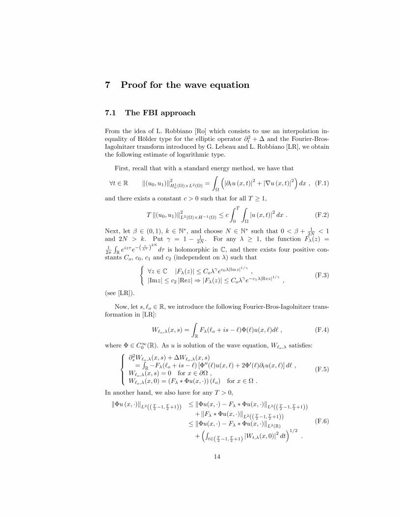
7 Proof for the wave equation

7.1 The FBI approach

From the idea of L. Robbiano [Ro] which consists to use an interpolation in-equality of Hölder type for the elliptic operator @2t + � and the Fourier-Bros-Iagolnitzer transform introduced by G. Lebeau and L. Robbiano [LR], we obtainthe following estimate of logarithmic type.

First, recall that with a standard energy method, we have that

8t 2 R k(u0; u1)k2H10 ()�L2()

=

Z

�j@tu (x; t)j2 + jru (x; t)j2

�dx , (F.1)

and there exists a constant c > 0 such that for all T � 1,

T k(u0; u1)k2L2()�H�1() � cZ T

0

Z

ju (x; t)j2 dx . (F.2)

Next, let � 2 (0; 1), k 2 N�, and choose N 2 N� such that 0 < � + 12N < 1

and 2N > k. Put = 1 � 12N . For any � � 1, the function F�(z) =

12�

RR e

iz�e�(�� )

2N

d� is holomorphic in C, and there exists four positive con-stants Co, c0, c1 and c2 (independent on �) such that(

8z 2 C jF�(z)j � Co� ec0�jImzj1=

,jImzj � c2 jRezj ) jF�(z)j � Co� e�c1�jRezj

1=

,(F.3)

(see [LR]).

Now, let s; `o 2 R, we introduce the following Fourier-Bros-Iagolnitzer trans-formation in [LR]:

W`o;�(x; s) =

ZRF�(`o + is� `)�(`)u(x; `)d` , (F.4)

where � 2 C10 (R). As u is solution of the wave equation, W`o;� satis�es:8>><>>:@2sW`o;�(x; s) + �W`o;�(x; s)=RR�F�(`o + is� `) [�

00(`)u(x; `) + 2�0(`)@tu(x; `)] d` ,W`o;�(x; s) = 0 for x 2 @ ,W`o;�(x; 0) = (F� � �u(x; �)) (`o) for x 2 .

(F.5)

In another hand, we also have for any T > 0,

k�u (x; �)kL2((T2 �1;T2 +1)) � k�u(x; �)� F� � �u(x; �)kL2((T2 �1;T2 +1))+ kF� � �u(x; �)kL2((T2 �1;T2 +1))

� k�u(x; �)� F� � �u(x; �)kL2(R)+�R

t2(T2 �1;T2 +1)

jWt;�(x; 0)j2 dt�1=2

.

(F.6)

14

Denoting F (f) the Fourier transform of f , by using Parseval equality and

F (F�) (�) = e�(�� )

2N

, one obtain

k�u(x; �)� F� � �u(x; �)kL2(R)= 1p

2�kF (�u(x; �)� F� � �u(x; �))kL2(R)

= 1p2�

�RR

����1� e�( �� )

2N�F (�u(x; �)) (�)

���2 d��1=2� C

�RR

���� �� �k F (�u(x; �)) (�)���2 d��1=2 because k < 2N

� C 1��k

�RR

��F �@kt (�u(x; �))� (�)��2 d��1=2 because � <

� C 1��k

@kt (�u(x; �)) L2(R) .

(F.7)

Therefore, from (F.6) and (F.7), one gets

k�u (x; �)kL2((T2 �1;T2 +1))� C 1

��k

@kt (�u(x; �)) L2(R) + �Rt2(T2 �1;T2 +1) jWt;�(x; 0)j2 dt�1=2

.(F.8)

Now, recall that from the Cauchy�s theorem we have:

Proposition 6 .- Let f be a holomorphic function in a domain D � C.Let a; b > 0, z 2 C. We suppose that

Do =�(x; y) 2 R2 ' C n jx� Rezj � a; jy � Imzj � b

� D ,

then

f (z) =1

�ab

Z Zj x�R eza j2+j y�Im zb j2�1

f (x+ iy) dxdy .

Choosing z = t 2�T2 � 1;

T2 + 1

�� R and x+ iy = `o + is, we deduce that

jWt;�(x; 0)j � 1�ab

Rj`o�tj�a

Rjsj�b jW`o+is;�(x; 0)j d`ods

� 1�ab

Rj`o�tj�a

Rjsj�b jW`o;�(x; s)j dsd`o

� 2�pab

�Rj`o�tj�a

Rjsj�b jW`o;�(x; s)j

2dsd`o

�1=2,

(F.9)

and with a = 2b = 1,Rt2(T2 �1;

T2 +1)

jWt;�(x; 0)j2 dt

�Rt2(T2 �1;

T2 +1)

�Rj`o�tj�1

Rjsj�1=2 jW`o;�(x; s)j

2dsd`o

�dt

�Rt2(T2 �1;

T2 +1)

R`o2(T2 �2;

T2 +2)

Rjsj�1=2 jW`o;�(x; s)j

2dsd`odt

� 2R`o2(T2 �2;

T2 +2)

Rjsj�1=2 jW`o;�(x; s)j

2dsd`o .

(F.10)

15

Consequently, from (F.8), (F.10) and integrating over , we get the existenceof C > 0 such thatR

Rt2(T2 �1;

T2 +1)

j�(t)u(x; t)j2 dtdx� C 1

�2�k

R

RR

��@kt (� (t)u(x; t)))��2 dtdx+4R`o2(T2 �2;

T2 +2)

�R

Rjsj�1=2 jW`o;�(x; s)j

2dsdx

�d`o .

(F.11)

Now recall the following quanti�cation result for unique continuation of ellipticequation with Dirichlet boundary condition.

Proposition 7 .- Let be a bounded open set in Rn, n � 1, eitherconvex or C2 and connected. Let E � be a measurable set with positivemeasure. Let f = f (x; s) 2 L2 (� (�1; 1)). Then there exists ec > 0 such thatfor all w = w (x; s) 2 H2 (� (�1; 1)) solution of�

@2sw +�w = f in � (�1; 1) ,w = 0 on @� (�1; 1) ,

for all " > 0, we have :Rjsj�1=2

Rjw (x; s)j2 dxds

� eceec="��Rjsj�1 RE jw (x; s)j dxds�2 + Rjsj�1 R jf (x; s)j2 dxds�+e�4c0="

Rjsj�1

Rjw (x; s)j2 dxds .

Applying to W`0;�, from (F.5) we deduce that for all " > 0,Rjsj�1=2

RjW`0;�(x; s)j

2dxds

� e�4c0="Rjsj�1

RjW`0;�(x; s)j

2dxds

+eceec=" �Rjsj�1 R! jW`0;�(x; s)j dxds�2

+eceec=" Rjsj�1 R ��RR�F�(`0 + is� `)[�00(`)u(x; `) + 2�0(`)@tu(x; `)] d`j2 dxds

���2 dxds .(F.12)

Consequently, from (F.11) and (F.12), there exists a constant C > 0, such thatfor all " > 0,R

Rt2(T2 �1;

T2 +1)

j�(t)u(x; t)j2 dtdx� C 1

�2�k

R

RR

��@kt (� (t)u(x; t)))��2 dtdx+4e�4c0="

R`o2(T2 �2;

T2 +2)

�Rjsj�1

RjW`0;�(x; s)j

2dxds

�d`o

+4CeC="R`o2(T2 �2;

T2 +2)

�Rjsj�1

REjW`0;�(x; s)j dxds

�2d`o

+4Ceec=" R`o2(T2 �2;

T2 +2)

�Rjsj�1

R

��RR�F�(`0 + is� `)

[�00(`)u(x; `) + 2�0(`)@tu(x; `)] d`j2 dxds�d`o .

(F.13)

16

Let de�ne � 2 C10 (R) more precisely now: we choose � 2 C10 ((0; T )), 0 �� � 1, � � 1 on

�T4 ;

3T4

�. Furthermore, let K =

�0; T4

�[�3T4 ; T

�such

that supp(�0) = K and supp(�00) � K. Let K0 =�3T8 ;

5T8

�. In partic-

ular, dist(K;Ko) =T8 . Let de�ne T > 0 more precisely now: we choose

T > 16max (1; 1=c2) in order that�T2 � 2;

T2 + 2

�� K0 and dist(K;Ko) � 2

c2.

Now, we will choose `0 2�T2 � 2;

T2 + 2

�� K0 and s 2 [�1; 1]. Consequently,

for any ` 2 K, j`0 � `j � 2c2� 1

c2jsj and it will imply from the second line of

(F.3) that

8` 2 K jF�(`o + is� `)j � A� e�c1�(T8 )

1=

. (F.14)

Till the end of the proof, C and respectively CT will denote a generic positiveconstant independent of " and � but dependent on and respectively (; T ),whose value may change from line to line.

The �rst term in the right hand side of (F.13) becomes, using (F.1),

1

�2�k

Z

ZR

��@kt (� (t)u(x; t)))��2 dtdx � CT 1

�2�kk(u0; u1)k2D(Ak�1) . (F.15)

The second term in the right hand side of (F.13) becomes, using the �rst lineof (F.3),

e�4c0="R`o2(T2 �2;

T2 +2)

�Rjsj�1

RjW`0;�(x; s)j

2dxds

�d`o

��Co�

e�c0�2e�4c0="

R`o2(T2 �2;

T2 +2)

�Rjsj�1

R

���R T0 ju(x; `)j d`���2 dxds�� CT�2 e2�c0e�4c0=" k(u0; u1)k2H1

0 ()�L2().

(F.16)The third term in the right hand side of (F.13) becomes, using the �rst line of(F.3),

eC="R`o2(T2 �2;

T2 +2)

�Rjsj�1

REjW`0;�(x; s)j dxds

�2d`o

��Co�

e�c0�2eC="

R`o2(T2 �2;

T2 +2)

hRjsj�1

RE

���R T0 ju(x; `)j d`��� dxdsi2 d`o� C�2 eC�eC="

�RE

R T0ju(x; t)j dtdx

�2.

(F.17)The fourth term in the right hand side of (F.13) becomes, using (F.14) and thechoice of �,

eec=" R`o2(T2 �2;

T2 +2)

�Rjsj�1

R

��RR�F�(`0 + is� `)

[�00(`)u(x; `) + 2�0(`)@tu(x; `)] d`j2 dxds�d`o

� C�A� e�c1�(

T8 )

1= �2eec=" R

��RK(ju(x; `)j+ j@tu(x; `)j) d`

��2 dx� C�2 e�2c1�(T8 )

1=

eec=" k(u0; u1)k2H10 ()�L2()

.

(F.18)

17

We �nally obtain from (F.15), (F.16), (F.17), (F.18) and (F.13), thatR

Rt2(T2 �1;

T2 +1)

j�(t)u(x; t)j2 dtdx� CT 1

�2�kk(u0; u1)k2D(Ak�1)

+CT�2 e2�c0e�4c0=" k(u0; u1)k2H1

0 ()�L2()

+C�2 eC�eC="�R

E

R T0ju(x; t)j dtdx

�2+C�2 e�2c1�(

T8 )

1=

eec=" k(u0; u1)k2H10 ()�L2()

.

(F.19)

We begin to choose � = 1" in order thatR

Rt2(T2 �1;

T2 +1)

j�(t)u(x; t)j2 dtdx� "2�kCT k(u0; u1)k2D(Ak�1)

+e�2c0=" 1"2 CT k(u0; u1)k

2H10 ()�L2()

+eC="C�R

E

R T0ju(x; t)j dtdx

�2+C 1

"2 exp���2c1

�T8

�1= + ec� 1

"

�k(u0; u1)k2H1

0 ()�L2().

(F.20)

We �nally need to choose T > 16max (1; 1=c2) large enough such that

�2c1�T

8

�1= + ec � �1

that is 8�1+ec2c1

� � T , to deduce the existence of C > 0 such that for any

" 2 (0; 1),R

Rt2(T2 �1;

T2 +1)

ju(x; t)j2 dtdx �R

Rt2(T2 �1;

T2 +1)

j�(t)u(x; t)j2 dtdx� C"2�k k(u0; u1)k2D(Ak�1)

+CeC="�R

E

R T0ju(x; t)j dtdx

�2.

(F.21)Now we conclude from (F.2), that there exist a constant c > 0 and a time T > 0large enough such that for all " > 0 we have

k(u0; u1)k2L2()�H�1()

� ec="�R

E

R T0ju(x; t)j dtdx

�2+ "2�k k(u0; u1)k2D(Ak�1) .

(F.22)

Finally, we choose

" =

1

2

k(u0; u1)kL2()�H�1()

k(u0; u1)kD(Ak�1)

!1=(�k).

18

7.2 The resolvent approach

We consider the damped wave equation8<: @2t y ��y + 1E@ty = 0 in � (0;+1) ,y = 0 on @� (0;+1) ,

(y; @ty) (�; 0) = (u0; u1) ,

which can be rewritten as follows� �x(t) = Bx(t) , t � 0 ,x(0) = x0 , x0 2 X ,

where B is the operator on X = H10 ()� L2 () de�ned by�

D (B) =�(u0; u1) 2 H1

0 ()� L2 () ;�u0 2 L2 () ; u1 2 H10 ()

B (u0; u1) = (u1;�u0 � 1Eu1) 8 (u0; u1) 2 D (B) .

Recall some de�nitions set up when X is a Hilbert space. The resolventoperator of B is de�ned by

�(B) � C �! L (B)� 7�! R (�;B) = (�Id�B)�1 .

Here B is an operator with domain D (B) in a Hilbert space X. We say that �,� 2 C, belongs to the resolvent set �(B) of B if the three following conditionsholds: �Id � B is bijective from D (B) to X; (�Id�B)�1 : X ! D (B) iscontinuous (that is (�Id�B)X = X); the domain of (�Id�B)�1 is dense inX (or the domain of �Id�B is dense in X that is (�Id�B)X = X).

�(B) =n� 2 C;�Id�B is bijective, (�Id�B)X = X, (�Id�B)X = X

o.

The set complementary to the resolvent (in the complex plane) is called thesprectrum of the operator B and denoted � (B), that is � (B) = C n�(B) .If E� = fu 2 D (B) ;Bu = �ug 6= f0g, then � is an eigenvalue of B. Further,

E� is called the eigenspace corresponding to � and the solution u is called aneigenvector of B corresponding to the eigenvalue �. The dimension of E� iscalled the multiplicity of the eigenvalue �. (If ej is associated to the eigenvalue�j , j 2 f1; 2g, then e1 and e2 are linearly independent for �1 6= �2).The point spectrum is the set of eigenvalues of the operator. It is denoted

�p (B).If X is �nite dimension, then �p (B) = � (B).

19

We de�ne the continuous spectrum of B, denoted �c (B), as follows � (B) =�c (B) [ �p (B). Finally, we de�ne the residual spectrum of B, denoted �r (B),as follows � (B) = �r (B) [ �c (B) [ �p (B) where �r, �c, �p are disjoint sets.

�p (B) = f� 2 C;�Id�B is not bijectiveg ,�c (B) =

n� 2 C;�Id�B is bijective, (�Id�B)X 6= X, (�Id�B)X = X

o,

�r (B) =n� 2 C;�Id�B is bijective, (�Id�B)X 6= X

o.

Theorem 8 .- Let (T (t))t�0 be a bounded C0�semigroup on a Banachspace X with generator B. Suppose that iR is contained in the resolvent set�(B) of B. Then T (t)B�1 ! 0; t!1 .

In other words, all classical solutions to the abstract Cauchy problem� �x(t) = Bx(t) , t � 0 ,

x(0) = x0 ,

given by x(t) = T (t)x0, t � 0, x0 2 D(B), converge uniformly (on the unit ballof D(B) with the graph norm) to zero at in�nity if B satis�es the assumptionsof the above Theorem 8.

Batty-Duyckaerts [BD] proves that iR � �(B) is a necessary and su¢ cientcondition to get

T (t)B�1 ! 0; t ! 1 . The long time asymptotic behaviorcan also be deduced by means of LaSalle invariance principle.

DenoteR (�;B) = (�Id�B)�1 , � 2 iR .

M (�) = max�2[��;�]

kR (i� ; B)k , � � 0 .

Theorem 9 .- Let (T (t))t�0 be a bounded C0�semigroup on a Banachspace X with generator B, such that iR � �(B). If M (�) � Cexp(C�) forsome constant C > 0, then

8k � 1, 9Ck > 0, kx(t)k �Ck

(log (2 + t))kkx0kD(Bk) .

This is a corollary of a theorem of Batty-Duyckaerts [BD]. The case whereX is a Hilbert space was established by Burq-Lebeau [Bu]-[Le].

Let f = (f0; f1) 2 H10 ()� L2 () and u = (u0; u1) 2 D(B). The following

equation(i�Id�B)u = f

20

is equivalent to

i� (u0; u1)� (u1;�u0 � 1Eu1) = (f0; f1)

that isu1 = i�u0 � f0 and ��u0 + i�u1 + 1Eu1 = f1 .

Then, u0 2 H2 \H10 () and

��u0 � �2u0 + i�1Eu0 = f1 + 1Ef0 + i�f0 in .

Let w (x; s) = e�su0 (x). Then w 2 H2 (� (�1; 1)) and solves�@2sw +�w � i�1Ee�su0 = �e�s (i�f0 + 1Ef0 + f1) in � (�1; 1) ,w = 0 on @� (�1; 1) .

Now we apply the following result.

Proposition 10 .- Let be a bounded open set in Rn, n � 1, eitherconvex or C2 and connected. Let E � be a measurable set with positivemeasure. Let f = f (x; s) 2 L2 (� (�1; 1)). Then there exists ec > 0 such thatfor all w = w (x; s) 2 H2 (� (�1; 1)) solution of�

@2sw +�w = f in � (�1; 1) ,w = 0 on @� (�1; 1) ,

for all " > 0, we have :Rjsj�1=2

Rjw (x; s)j2 dxds

� eceec="��Rjsj�1 RE jw (x; s)j dxds�2 + Rjsj�1 R jf (x; s)j2 dxds�+e�4c0="

Rjsj�1

Rjw (x; s)j2 dxds .

We deduce thatRjsj�1=2

Rje�su0 (x)j2 dxds

� eceec=" �Rjsj�1 RE je�su0 (x)j dxds�2+eceec=" Rjsj�1 R ji�1Ee�su0 + e�s (i�f0 + 1Ef0 � f1)j2 dxds+e�4c0="

Rjsj�1

Rje�su0 (x)j2 dxds .

On the other hand, we have the following estimate.Rjsj�1

Rji�1Ee�su0 + e�s (i�f0 + 1Ef0 � f1)j2 dxds

� CeCj� j�j� jREju0 (x)j2 dx+

Rjf0 (x)j2 dx+

Rjf1 (x)j2 dx

�.

21

Therefore

e�j� jRju0 (x)j2 dx

� eceec="CeCj� j �j� j REju0 (x)j2 dx+

Rjf0 (x)j2 dx+

Rjf1 (x)j2 dx

�+e�4c0="e2j� j

Rju0 (x)j2 dx .

FinallyZ

ju0 (x)j2 dx � CeCj� j�j� jZE

ju0 (x)j2 dx+Z

jf0 (x)j2 dx+Z

jf1 (x)j2 dx�.

On another hand,

��u0 + i�u1 + 1Eu1 = f1 and u1 = i�u0 � f0

imply using Cauchy-Schwarz inequality, thatZ

jru0 (x)j2 dx � C��j� j2 + 1

�Z

ju1 (x)j2 dx+Z

jf1 (x)j2 dx�

and Z

ju1 (x)j2 dx � C�j� j2

Z

ju0 (x)j2 dx+Z

jf0 (x)j2 dx�.

In the same way but with

��u0 � �2u0 + i�1Eu0 = f1 + 1Ef0 + i�f0 ,

using the imaginary part, we get

j� jREju0 (x)j2 dx � 2CeCj� j

��j� j2 + 1

� Rjf0 (x)j2 dx+

Rjf1 (x)j2 dx

�+ 12CeCj�j

Rju0 (x)j2 dx .

We conclude that

k(u0; u1)kH10 ()�L2()

� CeC� k(f0; f1)kH10 ()�L2()

, � 2 [��; �]

that isM (�) � CeC� .

By application of Theorem 9,

8k � 1, 9Ck > 0, k(y; @ty) (�; t)kH10 ()�L2()

� Ck

(log (2 + t))kk(u0; u1)kD(Bk) .

This is equivalent to the following observation estimate: 8k � 1, 9Ck > 0,

k(y; @ty) (�; 0)k2H10 ()�L2()

� h2 k(u0; u1)k2D(Bk)+2

Z exp��

Ckh

�1=k�0

ZE

j@tyj2 dxdt .

22

Finally, ( Ck(log(2+t))2k

= h2 ,exph�

Ckh2

�1=(2k)i= 2 + t), 8k � 1, 9Ck > 0,

k(u0; u1)k2H10 ()�L2()

� 4Z exp

24 Ck k(u0;u1)kD(Bk)k(u0;u1)kH1

0()�L2()

!1=k35

0

ZE

j@tyj2 dxdt .

By a classical way, we get: 8k � 1, 9Ck > 0,

k(u0; u1)k2L2()�H�1() � 4Z exp

24 Ck k(u0;u1)kD(Bk�1)k(u0;u1)kL2()�H�1()

!1=k35

0

ZE

jyj2 dxdt

where D�B0�= H1

0 () � L2 (). Notice that D�Ak�= D

�Bk�. Going back

to the wave equation by a decomposition method, we obtain: 9C > 0, 8k � 1,9Ck > 0,

k(u0; u1)k2L2()�H�1() � CZ exp

24 Ck k(u0;u1)kD(Ak�1)k(u0;u1)kL2()�H�1()

!1=k35

0

ZE

juj2 dxdt .

Therefore

k(u0; u1)k2D(Ak�1) � Ck(u0; u1)k2D(Ak�1)

k(u0; u1)k2L2()�H�1()

Z exp

24 Ck k(u0;u1)kD(Ak�1)k(u0;u1)kL2()�H�1()

!1=k35

0

ZE

juj2 dxdt

which implies

k(u0; u1)k2D(Ak�1) � CZ exp

24 Ck k(u0;u1)kD(Ak�1)k(u0;u1)kL2()�H�1()

!1=k35

0

ZE

juj2 dxdt .

References

[AE] J. Apraiz, L. Escauriaza, Null-control and measurable sets.ESAIM:COCV. To appear.

[AEWZ] J. Apraiz, L. Escauriaza, G. Wang, C. Zhang, Observability inequali-ties and measurable sets. To appear.

[BLR] C. Bardos, G. Lebeau, J. Rauch, Sharp su¢ cient conditions for the ob-servation, control and stabilization of waves from the boundary, SIAMJ. Control Optim., 30, 5, (1992), 1024�1065.

23

[BD] C. Batty, T. Duyckaerts, Non-uniform stability for bounded semi-groups on Banach spaces. J. Evol. Equ. 8 (2008), no. 4, 765�780.

[BT] C. Bardos and L. Tartar, Sur l�unicité retrograde des équationsparaboliques et quelques questions voisines, Arch. Rational Mech.Anal. 50 (1973), 10�25.

[Bu] N. Burq, Décroissance de l�énergie locale de l�équation des ondes pourle problème extérieur et absence de résonance au voisinage du réel,Acta Math. 180 1 (1998), 1�29.

[H] A. Haraux, Stabilization of trajectories for some weakly damped hy-perbolic equations, J. Di¤. Equ. 59 (1985), 145�154.

[Le] G. Lebeau, Équation des ondes amorties. In Algebraic and geometricmethods in mathematical physics (Kaciveli, 1993), vol. 19 of Math.Phys. Stud. Kluwer Acad. Publ. Dordrecht, 1996, pp. 73�109.

[LR] G. Lebeau and L. Robbiano, Stabilisation de l�équation des ondes parle bord, Duke Math. J. 86 (1997), 465�491.

[MV] E. Malinnikova, S. Vessella, Quantitative uniqueness for elliptic equa-tions with singular lower order terms, Math. Ann. 353 (2012), no.4,1157�1181.

[Ro] L. Robbiano, Fonction de coût et contrôle des solutions des équationshyperboliques, Asymptotic Anal. 10 (1995), 95�115.

[P1] K. D. Phung, Observability and control of Schrödinger equations.SIAM J. Control Optim. 40 (2001), no. 1, 211�230.

[P2] K. D. Phung, Wave, damped wave and observation. Some problems onnonlinear hyperbolic equations and applications, 386�412, Ser. Con-temp. Appl. Math. CAM, 15, Higher Ed. Press, Beijing, 2010.

[PW] K. D. Phung, G. Wang. An observability estimate for parabolic equa-tions from a measurable set in time and its applications. J. Eur. Math.Soc. To appear.

[R] R. Regbaoui, Unique continuation from sets of positive measure. Carle-man estimates and applications to uniqueness and control theory (Cor-tona, 1999), 179�190, Progr. Nonlinear Di¤erential Equations Appl.,46, Birkhäuser Boston, Boston, MA, 2001.

[Ru] D. Russell, Controllability and stabilizability theory for linear partialdi¤erential equations: recent progress and open questions. SIAM Rev.20 (1978), no. 4, 639�739.

[V] S. Vessella, A continuous dependence result in the analytic continua-tion problem. Forum Math. 11 (1999), no. 6, 695�703.

24