Submitted 23 October 2018Accepted 19 December 2018Published 22 January 2019

Corresponding authorZhitao Zhang, zhitaozhang@126.com

Academic editorTimothy Scheibe

Additional Information andDeclarations can be found onpage 20

DOI 10.7717/peerj.6310

Copyright2019 Wang et al.

Distributed underCreative Commons CC-BY 4.0

OPEN ACCESS

Quantitatively estimating main soilwater-soluble salt ions content based onVisible-near infrared wavelength selectedusing GC, SR and VIPHaifeng Wang1,2,*, Yinwen Chen3,*, Zhitao Zhang1,2, Haorui Chen4,Xianwen Li2, Mingxiu Wang5 and Hongyang Chai2

1Key Laboratory of Agricultural Soil and Water Engineering in Arid and Semiarid Areas, Ministry ofEducation, Northwest A&F University, Yangling, Shaanxi, China

2College of Water Resources and Architectural Engineering, Northwest A&F University, Yangling, Shaanxi,China

3Department of Foreign Languages, Northwest A&F University, Yangling, Shaanxi, China4Department of Irrigation and Drainage, China Institute of Water Resources and Hydropower Research,Beijing, China

5Department of Civil and Environmental Engineering, University of California, Irvine, CA, USA*These authors contributed equally to this work.

ABSTRACTSoil salinization is the primary obstacle to the sustainable development of agricultureand eco-environment in arid regions. The accurate inversion of themajor water-solublesalt ions in the soil using visible-near infrared (VIS-NIR) spectroscopy techniquecan enhance the effectiveness of saline soil management. However, the accuracy ofspectral models of soil salt ions turns out to be affected by high dimensionality andnoise information of spectral data. This study aims to improve the model accuracyby optimizing the spectral models based on the exploration of the sensitive spectralintervals of different salt ions. To this end, 120 soil samples were collected fromShahaoqu Irrigation Area in Inner Mongolia, China. After determining the rawreflectance spectrum and content of salt ions in the lab, the spectral data were pre-treated by standard normal variable (SNV). Subsequently the sensitive spectral intervalsof each ion were selected using methods of gray correlation (GC), stepwise regression(SR) and variable importance in projection (VIP). Finally, the performance of bothmodels of partial least squares regression (PLSR) and support vector regression (SVR)was investigated on the basis of the sensitive spectral intervals. The results indicatedthat the model accuracy based on the sensitive spectral intervals selected using differentanalyticalmethods turned out to be different: VIPwas the highest, SR came next andGCwas the lowest. The optimal inversionmodels of different ionswere different. In general,both PLSR and SVR had achieved satisfactory model accuracy, but PLSR outperformedSVR in the forecasting effects. Great difference existed among the optimal inversionaccuracy of different ions: the predicative accuracy of Ca2+, Na+, Cl−, Mg2+ and SO4

2−

was very high, that of CO32− was high and K+ was relatively lower, but HCO3

− failed tohave any predicative power. These findings provide a new approach for the optimizationof the spectral model of water-soluble salt ions and improvement of its predicativeprecision.

How to cite this article Wang H, Chen Y, Zhang Z, Chen H, Li X, Wang M, Chai H. 2019. Quantitatively estimating mainsoil water-soluble salt ions content based on Visible-near infrared wavelength selected using GC, SR and VIP. PeerJ 7:e6310http://doi.org/10.7717/peerj.6310

Subjects Soil Science, Data Mining and Machine Learning, Natural Resource Management,Environmental Impacts, Spatial and Geographic Information ScienceKeywords Soil salinization, Water-soluble salt ions, VIS-NIR, GC, SR, VIP, Model

INTRODUCTIONSoil salinization, one of themost important causes of land desertification and deterioration,has posed serious threat to agricultural development and sustainable utilization of naturalresources (Shahid & Rahman, 2011;Abbas et al., 2013). 950million ha of soil worldwide hasbecome salinized (Schofield & Kirkby, 2003). Soil salinization is eroding and degeneratingthe arable soil at the speed of 10 ha/min (Graciela & Alfred, 2009). Soil remediation andmanagement are very difficult in China because of such complex natural factors as climate,terrain and geology, and human factors as unreasonable irrigation and disruption ofecological balance. The total area of saline soil in China is 36 million ha (Li et al., 2014),accounting for 4.88% of the total area available nationwide (The National Soil Survey Office,1998). Saline soil usually has a high concentration of salt ions with a series of effects onthe plants such as physiological draught, ion toxicity and metabolic disorder, thus forming‘‘salt damage’’ (Munns, 2002; Tavakkoli et al., 2011). In addition, one major cause of theinaccuracy of soil salinity spectral measurement is that pure salts seldom exist in the soilbecause of some trace salt ion elements are always fixed in soil crystals. Therefore, quickand accurate acquisition of the detailed information of the various salt ions content in thesoil can enhance the pertinence and effectiveness of saline soil management.

The traditional quantitative estimation of soil salt contents usually includes such stepsas field soil sampling in fixed points, experiments in the laboratory and comprehensivestatistical analysis (Urdanoz & Aragüés, 2011). Such a method is incapable of the dynamicmonitoring of saline soil in a large area because of its high consumption of time andenergy, small number of measuring points and poor representativeness (Ding & Yu, 2014).Compared with conventional laboratory analysis methods, remote sensing technologyhas been widely used due to its rich information, continuity, high precision and low cost(Ben-Dor, 2002; Viscarra Rossel et al., 2006; Viscarra Rossel & Behrens, 2010; Viscarra Rossel& Webster, 2012). The various soil constituents (contents of water, salt, organic matterand so forth) can be acquired conveniently from remote sensing data (Gomez, ViscarraRossel & McBratney, 2008; Yu et al., 2010; Periasamy & Shanmugam, 2017). Hence, withthe abundant spectral reflection information within the VIS-NIR intervals of soil salinity, itis feasible to improve the accuracy of soil salinization inversion (Al-Khaier, 2003; Ben-Doret al., 2009; Abbas et al., 2013).

The application of VIS-NIR spectral analysis technique has been proved effectivein improving the accuracy of quantitative estimation and eliminating the externaldisturbance to some extent (Dehaan & Taylor, 2002; Metternicht & Zinck, 2003; Fariftehet al., 2008). The univariate linear regression on the basis of soil salinity index developedfor CR (continuum removed) reflectance can be used as a method for soil salt contentestimation (Weng, Gong & Zhu, 2008). Due to the strong correlation between soil electricalconductivity (EC) and soil salinity, EC is also one of the important indicators for evaluating

Wang et al. (2019), PeerJ, DOI 10.7717/peerj.6310 2/26

soil salinization degree. A variety of approaches have been used to acquire the EC in thefield soil, including the partial least squares regression (PLSR) and multivariate adaptiveregression splines (MARS) (Volkan Bilgili et al., 2010; Nawar, Buddenbaum & Hill, 2015),logarithmic model (Xiao, Li & Feng, 2016a), Bootstrap-BP neural network model (Wanget al., 2018d) and satellite remote sensing technology (Nawar et al., 2014; Bannari et al.,2018). In addition, the differential transformation (Xia et al., 2017) and fractional derivative(Wang et al., 2017; Wang et al., 2018c) can fully utilize the potential spectral informationand enhance model accuracy. The methods of spectral classification (Jin et al., 2015) andwater influence elimination (Chen et al., 2016; Peng et al., 2016b; Yang & Yu, 2017) workwell in improving the quantitative inversion accuracy of soil salinity. Therefore, the remotesensing technique is reliable to inverse the soil salinity quantitatively on different scales.

The quantitative analysis of VIS-NIR spectral intervals can help evaluate the contentof some chemical elements (Viscarra Rossel et al., 2006; Farifteh et al., 2008; Cécillon et al.,2009; Ji et al., 2016) due to the different characteristic absorption spectrum in soil chemicalelements. Besides, there exists a correlation between some principal salt ions (Na+, Cl−)and spectral reflectance (Jiang et al., 2017). Therefore, VIS-NIR spectroscopy technique canbe used to obtain the contents of the soil salt ions to a certain extent. The spectral responsecharacteristics of mid-infrared (MIR) spectroscopy are better than those of VIS-NIRspectroscopy in predicting soil salinity information, the latter has high predicting accuracyof the total salts content, HCO3

−, SO42− and Ca2+, followed by Mg2+, Cl− and Na+

(Peng et al., 2016a). The spectral models have satisfactory prediction of the SAR (sodiumabsorption ratio) of soil salinization evaluation parameter, which is composed of thecontents of Ca2+, Mg2+ and Na+ (Xiao, Li & Feng, 2016b). Qu et al. (2009) found that thecontents of the total salt, SO4

2−, pH and K++Na+ have a higher inversion accuracy usingspectral data to create PLSR model. The different pretreatment of the different ion modelsvaries by creating and analyzing PLSR model that demonstrates relatively good predictiveeffects like ion contents of Ca2+, Mg2+, SO4

2−, Cl−, and HCO3− (Dai et al., 2015). Overall,

PLSR is a frequently used and robust linear model for quantitative research because it hasinference capabilities which are useful to model a probable linear relationship betweenthe reflectance spectra and the salt ions content in soil. However, the non-uniform dataand non-linear reflectance in spectral information of some soil chemical elements lead tothe reduction in model accuracy (Viscarra Rossel & Behrens, 2010; Nawar, Buddenbaum &Hill, 2015). In particular, support vector regressions (SVR) based on kernel-based learningmethods has the ability to handle nonlinear analysis case with highmodel accuracy (Vapnik,1995; Peng et al., 2016a; Hong et al., 2018b). Over the past several decades, the use of SVRfor classification and regression has been extensively applied in soil VIS-NIR spectroscopy(Ben-Dor, 2002; Xiao, Li & Feng, 2016b; Hong et al., 2018a). Moreover, the SVR modelworks well in estimating the contents of K+, Na+, Ca2+ and SO4

2− in the soil (Wang et al.,2018a). Thus, the correct way of modeling helps to guarantee the model accuracy (Fariftehet al., 2007).

Many researches focused on the inversion of soil salinity using spectral information.Nevertheless, little research has explored the eight water-soluble salt ions (K+, Ca2+,Na+, Mg2+, Cl−, SO4

2−, HCO3− and CO3

2−) using spectral information in the soil. The

Wang et al. (2019), PeerJ, DOI 10.7717/peerj.6310 3/26

model fitting of ions and spectral information still needs improving (Farifteh et al., 2008;Peng et al., 2016a). Apart from the suitable multivariate statistical analysis method thatcan partly improve the inversion effects, reduction of redundant information is anotheridentified approach to further optimize the model (Bannari et al., 2018; Stenberg et al.,2010). Plenty of studies have demonstrated that spectral variable selection methods can notonly reduce the complexity of calibration models, but also improve the model predictiveperformance (Hong et al., 2018a). To select the optimal spectral variable subset, scholarshave investigated varied methods such as gray correlation (GC) (Li et al., 2016; Wanget al., 2018b), stepwise regression (SR) (Zhang et al., 2018) and variable importance inprojection (VIP) (Qi et al., 2017), and have achieved satisfactory effects. In addition, all thethree methods have been widely applied in many studies, such as plant physiology, foodengineering, mathematical statistics (Oussama et al., 2012;Maimaitiyiming et al., 2017; Liu,Yang & Wu, 2015). However, few studies have concentrated on the use of variable selectionalgorithms in the inversion of soil salt ions.

This study aims to: (1) build the optimal model of soil salt ions using VIS–NIRspectroscopy technique; (2) compare the models based on the sensitive spectral rangesselected using GC, SR andVIPmethods for different soil ions; (3) compare the performanceof PLSR and SVR models, and identify the optimal models for different ions.

MATERIALS AND METHODSStudy areaHetao Irrigation District (HID), with Yin Mountains at its north, the Yellow River at itssouth, Ulanbuh Desert at its west and Baotou at its east, lies in Bayannur League, InnerMongolia, China. It consists of irrigation areas of Ulan Buh, Jiefangzha, Yongji, Yichangand Urat, and it is China’s largest irrigation district with a total size of 5740 km2 (Yu etal., 2010). In addition, HID is an important production base of cereal and oil plants inChina with major crops of wheat, corn and sunflower. Shahaoqu Irrigation Area (SIA), atypical region of saline soil in HID, was chosen as the study area. SIA (107◦05′∼107◦10′E,40◦52′∼41◦00′N) is located in the central east of Jiefangzha Irrigation Area. SIA belongsto typical continental climate, having hot summers, chilly winters, rare precipitation andstrong evaporation. Its mean annual temperature, precipitation, potential evaporation isabout 7.1 ◦C, 155 mm and 2,000 mm, respectively. Physiographically, the mean elevationand slope of SIA are about 1,030 m and 1/10,000, respectively. According to the WorldReference Base for Soil Resources (WRB), the local soil texture is mainly silty clay loamwith varying degrees of saline soil. Over the years, due to its gentle terrain slope, poorgroundwater runoff, intense land surface evaporation and irrational farming activities,about 60% of the land within the district has been affected by various degree of salinization,which seriously restricted the agricultural development (Wu et al., 2008; Gao et al., 2015).

Sample collection and chemical analysisThe Hetao irrigation district administration gave field permit approval to us (NO.2017YFC0403302). To ensure the representativeness of soil samples, the samples wererandomly gathered from a total of 120 sampling units on a grid of 16 m ×16 m (because

Wang et al. (2019), PeerJ, DOI 10.7717/peerj.6310 4/26

Figure 1 Distribution of sampling sites in the study area. (A) Location map of Shahaoqu IrrigationArea. (B) Sampling location in Shahaoqu Irrigation Area.

Full-size DOI: 10.7717/peerj.6310/fig-1

the spatial resolution of GF-1 satellite imagery is 16 m) in the study area during October12∼22, 2017 (Fig. 1). In each unit, approximately 0.5 kg of topsoil (0–5 cm) was collected atfour randomly selected sampling sites and thenmixed thoroughly to obtain a representativesample. Overall, a total of 120 soil samples were acquired, and each sample was storedin a plastic bag, labeled and sealed. A portable global position system (GPS) was usedto determine the coordinates of sampling points. Subsequently, the soil samples weretransported to the lab to receive a series of such treatments as sufficient natural air-dryingfor two weeks and rubbing through a 2 mm sieve to exclude small stones and otherimpurities. Each sample was divided into two subsamples to be used for spectra collectionand physiochemical analysis.

Each 50 g of soil sample was put into a respective flask, and 250 ml of distilled water (theratio of water to soil is 5:1) were added into each flask. The water-soluble ion contents weremeasured in the filtrate obtained from full soaking, oscillation and filtration (Aboukila &Norton, 2017). Ca2+ and Mg2+ were measured using EDTA titration, Na+ and K+ flamephotometry, CO3

2− and HCO3− double indicator-neutralization titration, Cl− silver

nitrate titration, and SO42− EDTA indirect complexometry (Bao, 2000). The content of

CO32− was too low (approximately 0) in some soil samples because CO3

2− is liable tointegrate with Ca2+ andMg2+ as sediment in a weak alkaline solution (Table 1). Coefficientof variation (CV) reflects the degree of discreteness, and a positive correlation exists in twovariables. The high CV helps to build a robust model (Dai et al., 2015). The grading of CVshowed a wide range of variation among different ions, among which the ion contents ofK+, Na+ and SO4

2− are over 100%, showing a strong variability, and those of CO32−, Cl−,

Ca2+, Mg2+ and HCO3− are between 10% and 100%, having a moderate variability.

Wang et al. (2019), PeerJ, DOI 10.7717/peerj.6310 5/26

Table 1 Descriptive statistics of soil water-soluble salt ions content.

Statisticalindex

Minimum/g kg−1

Maximum/g kg−1

Mean/g kg−1

Standarddeviation

Coefficientof variation/%

CO32− 0.000 0.066 0.020 0.020 98.86

HCO3− 0.171 0.666 0.316 0.099 31.27

SO42− 0.047 40.892 9.073 10.828 119.34

Cl− 0.145 23.234 4.825 4.711 97.65Ca2+ 0.080 4.111 0.697 0.669 95.95Mg2+ 0.039 1.952 0.706 0.606 85.91K+ 0.001 5.727 0.936 1.358 145.14Na+ 0.016 23.035 5.014 5.563 110.94

Laboratory spectral measurements and pretreatmentsThe soil samples were put into black vessels with a diameter of 10 cm and depth of 2 cm forspectral data collection and the surfaceswere smoothedwith a straightedge in the laboratory.The spectral data of the soil samples were measured using ASD (Analytical Spectral Devices,Inc., Boulder, CO, USA) FieldSpec R©3 spectrometer with spectral range from 350–2,500nm. This instrument is equipped with two sensors whose spectral resolutions are 1.4 nmand 2 nm, for the region of 350–1,000 nm and 1,000–2,500 nm, respectively. The spectraldata was measured in a dark room with the light sources which have halogen lamps of 50W, 50 cm from the sample soil surfaces, and 30◦ incident angle to reduce the effects ofexternal factors to the minimum. The field angle of fiber-optics probe is 5◦, and it is 15 cmfrom the sample soil surface. The light source and spectrometer had been fully preheated,and the spectrometer had been corrected with a standardized white panel (99% reflectance)prior to each measurement to reduce measurement error. Each sample soil was measuredin four directions (3 turns, each is 90◦), the spectrum was collected five times in eachdirection, and altogether there were 20 curves of the spectrum (Hong et al., 2018b). Thesecurves were used as the raw spectral reflectance (Rraw) after having the arithmetic mean inViewSpecPro software version 6.0. The gaps of the spectral curves near 1,000 nm and 1,800nm were corrected using the Splice Correction function (Xiao, Li & Feng, 2016a).

The fluctuation would affect the accuracy of subsequent modeling because of suchdisturbance as the external environment, instrument noise and random error in spectraldata collection. In general, a series of effective pretreatment, including smoothing,resampling and transformation etc., can eliminate the external noise to some degree,and then enhance the spectral characteristics (Ding et al., 2018). Therefore, it is necessaryto pretreat Rraw in the following steps. (i) The marginal wavelength (350–399 nm and2,401–2,500 nm) of higher noise in each soil sample was removed, then remaining spectrumdata was smoothed with filter method (window size is 5 and polynomial order is 2) usingSavitzky-Golay (SG) (Savitzky & Golay, 1964) via Origin Pro software version 2017SR2.(ii) The spectral data between 400 and 2,400 nm was resampled with a 10 nm of sampleinterval to keep the spectral features and remove redundant information (Xu et al., 2016).A new spectral curve consisting of 200 wave bands was obtained. (iii) The precise Rraw−SNV

was obtained by using the standard normal variable (SNV) to eliminate the effects of soil

Wang et al. (2019), PeerJ, DOI 10.7717/peerj.6310 6/26

Figure 2 Spectral curves of all soil samples. (A) Reflectance spectral curves. (B) Standard normal vari-able reflectance curves.

Full-size DOI: 10.7717/peerj.6310/fig-2

particle size, surface scattering and baseline shift on the spectrum data (Xiao, Li & Feng,2016b; Barnes, Dhanoa & Lister, 1989). The spectral curves of Rraw and Rraw−SNV are shownin Figs. 2A and 2B. Notably, comparison indicated that the spectral curve in Fig. 2B wasmuch smoother than that in Fig. 2A, which made for the subsequent modeling.

Gray correlation (GC)The GC, as one grey system theory, seeks the primary and secondary relations and analyzesthe different effects of all the factors in a system (Deng, 1982; Li et al., 2016). Its calculationprocess is as follows: the reference sequence is X0={x0(t ),t = 1,2,...,n}, the comparativesequence is Xi = {xi(t ),t = 1,2,...,n}, and the formula of the gray correlation degree(GCD) between X0 and Xi is

GCD=1n

n∑t=1

γ (x0(t ),xi(t )) (1)

where γ (x0(t ),xi(t ))= minimint |x0(t )−xi(t )|+ρmaximaxt |x0(t )−xi(t )||x0(t )−xi(t )|+ρmaximaxt |x0(t )−xi(t )|

ρ is the distinguishing coefficient within [0,1] . ρ was set as 0.1 in this paper.The inconsistent dimension between the spectral data and the contents of different

ions has some effects on the data analysis. Therefore, normalizing the spectral datapreprocessing method can reduce these disadvantageous effects (Liu, Yang & Wu, 2015;Wang et al., 2018b). In this paper, the larger the GCD of a certain band is, the closer relationthe band and the ion content has, and vice versa.

Variable importance in projection (VIP)The VIP is a variable selection method based on PLSR (Oussama et al., 2012). Theexplanatory power of the independent variables to the dependent variables is achievedby calculating the VIP score. The independent variables are sequenced according to the

Wang et al. (2019), PeerJ, DOI 10.7717/peerj.6310 7/26

explanatory power (Qi et al., 2017). The VIP score for the j-th variable is given as:

VIPj =

√p∗

∑Ff=1SSYf ∗W2

jf

SSYtotal ∗F(2)

Where p is the number of independent variables; f is the total number of components;SSYf is the sum of squares of explained variance for the f -th component and p the numberof independent variables. SSYtotal is the total sum of squares explained of the dependentvariable. W2

jf gives the importance of the j-th variable in each f -th component. The highervalue VIPj has, the stronger explanatory power the independent variable has over thedependent variable. The VIP scores of independent variables have been recognized as auseful measure to identify important wavelengths when the score is more than 1 (Wold,Sjöström & Eriksson, 2001; Maimaitiyiming et al., 2017).

Model construction and validationTwo-thirds of the samples were used for modeling (n = 80) and one third for validation(n = 40) using Kennard-Stone (K-S) to calculate the Euclidean distance among differentsamples to ensure the statistical characteristics of modeling and the validation datasetsresembled that of the whole sample set (Kennard & Stone, 1969).

The PLSR and SVR models were applied to the quantitative inversion of differentwater-soluble salt ion contents in the saline soil in this paper. The PLSR model is a newstoichiometric statistical model. Compared with the traditional multivariate least squaresregression (MLSR), PLSR can overcome the multicollinearity among the variables, reducethe dimension, synthesize and filter the information, extract the aggregate variables withthe strongest explanatory power in the system, and exclude the noise with no explanatorypower (Wold, Sjöström & Eriksson, 2001). The optimal fitting model was built using thenumber of optimal principal components through full cross validation. SVR model isa new machine learning method based on the principle of structural risk minimizationprovided by the statistical learning theory. This model is characterized by its ability ofsolving such problems as limited sample size, nonlinear data processing and spatial patternrecognition of high-dimension data (Vapnik, 1995). During the modeling in this study,the type of SVR and kernel were set as epsilon-SVR and linear function, respectively; thepenalty parameter C and nuclear parameter g were acquired by a grid-searching techniqueand a leave-one-out cross validation procedure. The optimal values of C and g wereselected when the minimum RMSECV (root mean squared error of cross validation) wasproduced (Xiao, Li & Feng, 2016b). The two models were constructed and validated usingthe Unscrambler software version X10.4 (CAMO AS Oslo, Oslo, Norway).

Precision indices of determination coefficient of calibration (Rc2), determination

coefficient of prediction (Rp2), rootmean squared error (RMSE) and ratio of performance to

deviation (RPD) were used to evaluate the performance of these models. RPD classificationwas adopted to facilitate the interpretation of predictive results: a model is considered asexcellent when RPD ≥ 2.5, as very good when 2.0 ≤ RPD < 2.5, as good when 1.8 ≤ RPD<2.0, and as satisfactory when 1.4 ≤ RPD <1.8 and can only distinguish between high andlow values when 1.0 ≤ RPD <1.4 (Viscarra Rossel, Taylor & McBratney, 2007). Generally,

Wang et al. (2019), PeerJ, DOI 10.7717/peerj.6310 8/26

Figure 3 Correlation coefficients of soil water-soluble salt ions content with standard normal variablereflectance.

Full-size DOI: 10.7717/peerj.6310/fig-3

Table 2 Max correlation coefficient and band intervals of soil water-soluble salt ions content withstandard normal variable reflectance.

Water-solublesalt ions

Number ofsignificant bands

Maximum correlationcoefficient

Maximum correlationband intervals/nm

Ca2+ 190 −0.877 1,940∼1,950Cl− 192 −0.882 1,990∼2,000CO3

2− 146 0.552 1,870∼1,880HCO3

− 1 0.235 2,200∼2,210K+ 178 0.630 1,850∼1,860Mg2+ 186 −0.848 1,990∼2,000Na+ 181 −0.752 2,010∼2,020SO4

2− 178 0.749 1,860∼1,870

the most robust model would be the one with the largest Rc2, Rp

2 (approach to 1) and RPDvalue and the lowest RMSE value.

RESULTSCorrelation between water-soluble salt ions content and spectralreflectanceThe correlation coefficients (Pearson correlation) between each soil salt ion content andRraw−SNV in the range of 400–2,400 nm were tested with the significance level of P < 0.01(|r | = 0.234 or above). The curves of correlation coefficients of soil salt ions were plottedin Fig. 3 and the numbers of bands passing the significance test were counted in Table 2.The curve patterns of SO4

2−, Cl−, Ca2+, Mg2+, K+ and Na+ were similar (Fig. 3). From400 nm to about 550 nm, the correlation coefficients rose sharply from negative to positive,moved with a gentle depression until 1,400 nm, plummeted and surged up to 1,560 nm

Wang et al. (2019), PeerJ, DOI 10.7717/peerj.6310 9/26

Figure 4 Gray correlation degree (GCD) for soil water-soluble salt ions content with standard normalvariable reflectance.

Full-size DOI: 10.7717/peerj.6310/fig-4

(among the curves, the change of Ca2+ was the sharpest), and maintained a relativestable state to 1850 nm. And then from 1,850 to 2,400 nm, dramatic oscillating variationsalternated between rise and fall. In the intervals of 400–1,400 nm and 1,850–2,400 nm thecurve pattern of CO3

2− was similar to that of other ions such as SO42−. But between 1,400

nm and about 1,850 nm, the curve took on a unique pattern: sustained oscillating rise. Thecoefficient curve of HCO−3 displayed a smaller variation, smoothly fluctuating between−0.2 and 0.2. The complex variation of the coefficient curves of different ions revealed richspectral information.

Selection of characteristic wavelengthCharacteristic wavelength selection based on GC methodThe curves of gray correlation degree for soil water-soluble salt ions content and Rraw−SNV

were shown in Fig. 4. The correlation coefficient curves of the seven ions except CO32−

resembled those of the GCD of the Rraw−SNV. Generally, the curves exhibited patternsof ‘‘oscillatory rise, fluctuation, rapid rise and fall, and oscillatory fluctuation’’. The graycorrelation curves of CO3

2− followed a pattern of ‘‘ascending, plummeting, and smoothtransition’’. The analysis of the GC curve amplitude showed the amplitudes of Cl−, Mg2+

and Ca2+ were relatively large, and those of Na+, SO42−, K+ and HCO3

− were relativelysmall, and that of CO3

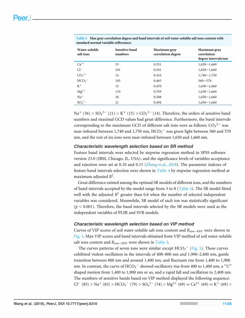
2− was relatively gentle.The order of the maximal GCD was: Cl− (0.561) > Mg2+ (0.559) > Ca2+ (0.551) > Na+

(0.508) > SO42− (0.494) > K+ (0.470) > HCO3

− (0.465) > CO32− (0.416). To ensure that

each salt ion had sensitive bands as far as possible, the GCD threshold value was set as 0.40to select the wavelength. The sensitive band was counted through gray correlation method(Table 3). The numbers of sensitive bands of different ions could be sequenced from thelargest to the smallest as follows: Mg2+ (110) > HCO3

− (105) > Cl− (101) > Ca2+ (53) >

Wang et al. (2019), PeerJ, DOI 10.7717/peerj.6310 10/26

Table 3 Max gray correlation degree and band intervals of soil water-soluble salt ions content withstandard normal variable reflectance.

Water-solublesalt ions

Sensitive bandnumbers

Maximum graycorrelation degree

Maximum graycorrelationdegree intervals/nm

Ca2+ 53 0.551 1,650∼1,660Cl− 101 0.561 1,650∼1,660CO3

2− 14 0.416 1,740∼1,750HCO3

− 105 0.465 560∼570K+ 15 0.470 1,650∼1,660Mg2+ 110 0.559 1,650∼1,660Na+ 36 0.508 1,650∼1,660SO4

2− 21 0.494 1,650∼1,660

Na+ (36) > SO42− (21) > K+ (15) > CO3

2− (14). Therefore, the orders of sensitive bandnumbers and maximal GCD values had great difference. Furthermore, the band intervalscorresponding to the maximum GCD of different salt ions were as follows: CO3

2− wasnear-infrared between 1,740 and 1,750 nm, HCO3

− was green light between 560 and 570nm, and the rest of six ions were near-infrared between 1,650 and 1,660 nm.

Characteristic wavelength selection based on SR methodFeature band intervals were selected by stepwise regression method in SPSS softwareversion 23.0 (IBM, Chicago, IL, USA), and the significance levels of variables acceptanceand rejection were set at 0.10 and 0.15 (Zhang et al., 2018). The parameter indexes offeature band intervals selection were shown in Table 4 by stepwise regression method atmaximum adjusted R2.Great difference existed among the optimal SRmodels of different ions, and the numbers

of band intervals accepted by the model range from 3 to 8 (Table 4). The SR model fittedwell with the adjusted R2 greater than 0.8 when the number of selected independentvariables was considered. Meanwhile, SR model of each ion was statistically significant(p < 0.001). Therefore, the band intervals selected by the SR models were used as theindependent variables of PLSR and SVR models.

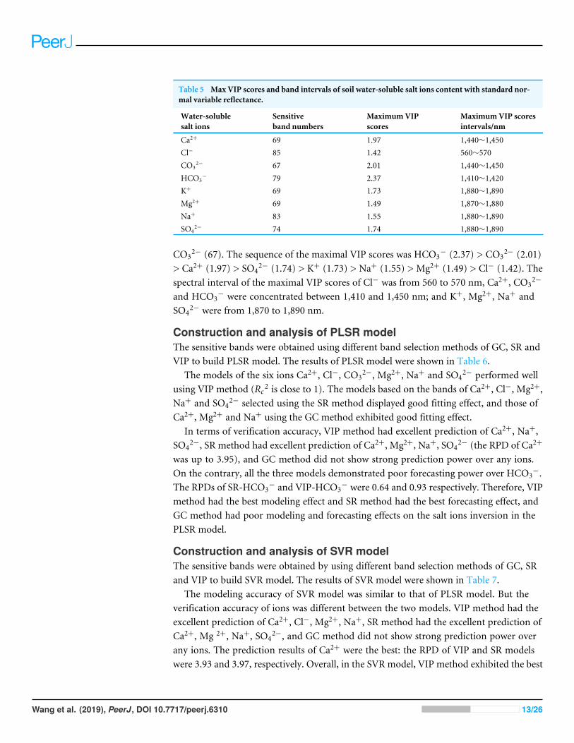
Characteristic wavelength selection based on VIP methodCurves of VIP scores of soil water-soluble salt ions content and Rraw−SNV were shown inFig. 5. Max VIP scores and band intervals obtained from VIP method of soil water-solublesalt ions content and Rraw−SNV were shown in Table 5.

The curves patterns of seven ions were similar except HCO3− (Fig. 5). These curves

exhibited violent oscillation in the intervals of 400–800 nm and 1,900–2,400 nm, gentletransition between 800 nm and around 1,400 nm, and fluctuant rise from 1,400 to 1,900nm. In contrast, the curve of HCO3

− showed oscillatory rise from 400 to 1,400 nm, a ‘‘U’’shaped motion from 1,400 to 1,900 nm or so, and a rapid fall and oscillation to 2,400 nm.The numbers of sensitive bands based on VIP method displayed the following sequence:Cl− (85) > Na+ (83) > HCO3

− (79) > SO42− (74) > Mg2+ (69) = Ca2+ (69) = K+ (69) >

Wang et al. (2019), PeerJ, DOI 10.7717/peerj.6310 11/26

Figure 5 The Variable importance in projection (VIP) scores for soil water-soluble salt ions contentwith standard normal variable reflectance.

Full-size DOI: 10.7717/peerj.6310/fig-5

Table 4 Parameter indexes of feature band intervals selection by stepwise regressionmethod.

Water-solublesalt ions

Sensitivebandnumbers

Bandintervals/nm

AdjustedR2

Standarderror

Sig.

Ca2+ 7 1,040∼1,050, 1,090∼1,100,1,900∼1,910, 1,920∼1,930,2,200∼2,210, 2,310∼2,320,2,370∼2,380

0.942 0.529 <0.001

Cl− 8 730∼740, 910∼920,1,890∼1,900, 1,970∼1,980,1,990∼2,000, 2,180∼2,190,2,200∼2,210, 2,290∼2,300

0.975 1.063 <0.001

CO32− 4 1,280∼1,290, 1,360∼1,370,

1,380∼1,390, 1,420∼1,4300.836 0.012 <0.001

HCO3− 3 2,200∼2,210, 2,260∼2,270,

2,290∼2,3000.934 0.085 <0.001

K+ 6 740∼750, 810∼820,1,160∼1,170, 1,890∼1,900,2,210∼2,220, 2,390∼2,400

0.817 0.706 <0.001

Mg2+ 6 1,130∼1,140, 1,930∼1,950,1,990∼2,000, 2,100∼2,110,2,170∼2,180

0.973 0.152 <0.001

Na+ 6 740∼750, 820∼830,1,860∼1,870, 2,210∼2,220,2,260∼2,270, 2,390∼2,400

0.942 1.812 <0.001

SO42− 6 610∼620, 1,140∼1,150,

1,960∼1,970, 2,210∼2,220,2,290∼2,300, 2,390∼2,400

0.947 3.255 <0.001

Wang et al. (2019), PeerJ, DOI 10.7717/peerj.6310 12/26

Table 5 Max VIP scores and band intervals of soil water-soluble salt ions content with standard nor-mal variable reflectance.

Water-solublesalt ions

Sensitiveband numbers

MaximumVIPscores

MaximumVIP scoresintervals/nm

Ca2+ 69 1.97 1,440∼1,450Cl− 85 1.42 560∼570CO3

2− 67 2.01 1,440∼1,450HCO3

− 79 2.37 1,410∼1,420K+ 69 1.73 1,880∼1,890Mg2+ 69 1.49 1,870∼1,880Na+ 83 1.55 1,880∼1,890SO4

2− 74 1.74 1,880∼1,890

CO32− (67). The sequence of the maximal VIP scores was HCO3

− (2.37) > CO32− (2.01)

> Ca2+ (1.97) > SO42− (1.74) > K+ (1.73) > Na+ (1.55) > Mg2+ (1.49) > Cl− (1.42). The

spectral interval of the maximal VIP scores of Cl− was from 560 to 570 nm, Ca2+, CO32−

and HCO3− were concentrated between 1,410 and 1,450 nm; and K+, Mg2+, Na+ and

SO42− were from 1,870 to 1,890 nm.

Construction and analysis of PLSR modelThe sensitive bands were obtained using different band selection methods of GC, SR andVIP to build PLSR model. The results of PLSR model were shown in Table 6.

The models of the six ions Ca2+, Cl−, CO32−, Mg2+, Na+ and SO4

2− performed wellusing VIP method (Rc

2 is close to 1). The models based on the bands of Ca2+, Cl−, Mg2+,Na+ and SO4

2− selected using the SR method displayed good fitting effect, and those ofCa2+, Mg2+ and Na+ using the GC method exhibited good fitting effect.

In terms of verification accuracy, VIP method had excellent prediction of Ca2+, Na+,SO4

2−, SR method had excellent prediction of Ca2+, Mg2+, Na+, SO42− (the RPD of Ca2+

was up to 3.95), and GC method did not show strong prediction power over any ions.On the contrary, all the three models demonstrated poor forecasting power over HCO3

−.The RPDs of SR-HCO3

− and VIP-HCO3− were 0.64 and 0.93 respectively. Therefore, VIP

method had the best modeling effect and SR method had the best forecasting effect, andGC method had poor modeling and forecasting effects on the salt ions inversion in thePLSR model.

Construction and analysis of SVR modelThe sensitive bands were obtained by using different band selection methods of GC, SRand VIP to build SVR model. The results of SVR model were shown in Table 7.

The modeling accuracy of SVR model was similar to that of PLSR model. But theverification accuracy of ions was different between the two models. VIP method had theexcellent prediction of Ca2+, Cl−, Mg2+, Na+, SR method had the excellent prediction ofCa2+, Mg 2+, Na+, SO4

2−, and GC method did not show strong prediction power overany ions. The prediction results of Ca2+ were the best: the RPD of VIP and SR modelswere 3.93 and 3.97, respectively. Overall, in the SVR model, VIP method exhibited the best

Wang et al. (2019), PeerJ, DOI 10.7717/peerj.6310 13/26

Table 6 Calibration and validation results of soil water-soluble salt ions content from the PLSR inver-sionmodels using the GC, SR and VIP wavelength selection methods.

Wavelengthselection methods

Water-solublesalt ions

Latentvariables

Calibrationsets

Validation sets

Rc2 Rp

2 RMSE/(g kg−1) RPD

Ca2+ 7 0.897 0.724 0.362 1.71Cl− 7 0.796 0.565 3.150 1.35CO3

2− 5 0.660 0.649 0.012 1.21HCO3

− 7 0.646 0.285 0.088 0.96K+ 1 0.388 0.258 1.209 0.85Mg2+ 6 0.891 0.767 0.295 1.99Na+ 7 0.840 0.805 2.589 1.88

Graycorrelation

SO42− 4 0.561 0.360 8.711 0.87

Ca2+ 7 0.965 0.937 0.168 3.95Cl− 2 0.861 0.729 2.434 1.80CO3

2− 4 0.685 0.742 0.010 1.80HCO3

− 3 0.340 0.154 0.094 0.64K+ 5 0.722 0.563 0.931 1.37Mg2+ 4 0.933 0.849 0.236 2.52Na+ 3 0.901 0.868 2.145 2.67

Stepwiseregression

SO42− 5 0.918 0.889 3.807 2.75

Ca2+ 3 0.909 0.865 0.249 2.57Cl− 4 0.930 0.862 1.725 2.48CO3

2− 9 0.865 0.617 0.012 1.44HCO3

− 9 0.704 0.263 0.090 0.93K+ 5 0.664 0.566 0.945 1.43Mg2+ 3 0.910 0.840 0.243 2.34Na+ 8 0.939 0.902 1.801 3.15

Variableimportanceinprojection

SO42− 8 0.919 0.872 4.038 2.75

performance for modeling and predicting the salt ions content, SR method was the second,and GC method was relatively poorer.

DISCUSSIONComparison among the results of different salt ions content inestimatingThe optimal band selection method varied in some degree from the optimal modelingmethod (Tables 6 and 7). The comparison was made between the measured value and theestimated value of all the ions concerned under the optimal model (Fig. 6). The sequenceof the forecasting power of the ions was Ca2+ > Na+ > Cl− > Mg2+ > SO4

2− > CO32− >

K+ > HCO3−, and it was the same as that of the modeling power.

Obviously, the verification result showed that most data points of the five ions, Ca2+,Na+, Cl−, Mg 2+ and SO4

2−, were concentrated near line 1:1. The optimal models ofthese five ions had very strong predicative power with the RPD above 2.5 (Tables 6 and 7).

Wang et al. (2019), PeerJ, DOI 10.7717/peerj.6310 14/26

Table 7 Calibration and validation results of soil water-soluble salt ions content from the SVR inver-sionmodels using the GC, SR and VIP wavelength selection methods.

Wavelengthselection methods

Water-solublesalt ions

Calibrationsets

Validation sets

Rc2 Rp

2 RMSE/(g kg−1) RPD

Ca2+ 0.910 0.752 0.337 1.73Cl− 0.652 0.500 3.275 1.05CO3

2− 0.688 0.664 0.012 1.14HCO3

− 0.563 0.328 0.083 0.70K+ 0.421 0.269 1.155 0.61Mg2+ 0.934 0.781 0.289 2.07Na+ 0.809 0.764 2.851 1.85

Graycorrelation

SO42− 0.565 0.397 9.046 0.52

Ca2+ 0.964 0.940 0.164 3.97Cl− 0.893 0.790 2.186 2.15CO3

2− 0.605 0.583 0.013 1.16HCO3

− 0.327 0.164 0.095 0.56K+ 0.717 0.578 0.874 1.26Mg2+ 0.936 0.875 0.214 2.75Na+ 0.903 0.864 2.171 2.61

Stepwiseregression

SO42− 0.915 0.893 3.862 2.71

Ca2+ 0.960 0.935 0.173 3.93Cl− 0.949 0.897 1.483 2.98CO3

2− 0.883 0.664 0.012 1.56HCO3

− 0.669 0.280 0.088 0.91K+ 0.645 0.565 0.888 1.23Mg2+ 0.965 0.877 0.214 2.51Na+ 0.958 0.872 2.211 2.76

Variableimportanceinprojection

SO42− 0.914 0.865 4.106 2.48

Compared with the previous researches, model prediction effects of K+ and Na+ (Qu et al.,2009); Ca2+, Na+ and Mg2+ (Viscarra Rossel & Webster, 2012); HCO3

−, Ca2+, Cl−, Mg2+

and SO42−(Dai et al., 2015); HCO3

−, Ca2+ and SO42− (Peng et al., 2016a); K+, Na+, Ca2+

and SO42− (Wang et al., 2018a) were satisfactory. Although the results of this study are

not exactly the same as these previous researches, it still shows the rationality own to someextent. In addition, this result shows that band selection has realized the goal of removingthe irrelevant information, and plays a major role in improving the inversion accuracy ofsalt ions.

In Fig. 6, the data points of CO32− and K+ were relatively dispersed in the verification

result. The CO32− had a relatively good predictive power (RPD = 1.80) and the K+ had

a normal predictive power (RPD = 1.43). Notably, HCO3− had no predicative power

(RPD = 0.96) because the slope was under the 1:1 line and the data points were mostdiscrete (Fig. 6D). The predicting effect of HCO3

− was different from that of Peng et al.(2016a) and Dai et al. (2015), but similar to that of Wang et al. (2018a). The cause of this

Wang et al. (2019), PeerJ, DOI 10.7717/peerj.6310 15/26

Figure 6 Validation of soil water-soluble salt ions content based on the best model. (A) Ca2+ with SR-SVR model. (B) Cl− with VIP-SVR model. (C) CO2−

3 with SR-PLSR model. (D) HCO−3 with GC-PLSRmodel. (E) K+ with VIP-PLSR model. (F) Mg2+ with SR-SVR model. (G) Na+ with VIP-PLSR model. (H)SO2−

4 with VIP-PLSR model.Full-size DOI: 10.7717/peerj.6310/fig-6

Wang et al. (2019), PeerJ, DOI 10.7717/peerj.6310 16/26

result needs to be further studied. Overall, it is vital to make some efforts to improve therobustness and accuracy of these ion models. Xiao, Li & Feng (2016b) failed to predictNa+, Mg 2+ and Ca2+, but applied the SVR model to forecasting SAR after the SNVtransformation and the performance was satisfactory (RPD = 2.13). Analogously, firstderivative reflectance (FDR) index was calculated to effectively predict SAR by Xiao, Li &Feng (2016a). In addition, Viscarra Rossel & Webster (2012) forecasted the content of Na+

after logarithmic pretreatment with VIS-NIR spectral technique (RPD = 2.10). Thus, saltion indexes construction and variable transformation processing are helpful approaches toimprove the correlation with the spectra so as to establish satisfactory models.

A little difference existed in the applicability between PLSR and SVRmodels on inversingthe content of ions. Both methods could produce satisfactory results in conformity withthat of Peng et al. (2016a). In addition, the optimal inversion models and predictionmodels for each ion were different: SR-PLSR model and SR-SVR model for Ca2+, VIP-SVR model and SR-PLSR model for CO3

2−, SR-PLSR model and VIP-PLSR model forK+, VIP-PLSR model and GC-PLSR model for HCO3

−, respectively. Among them, theperformance of the optimal inversion model of Ca2+ resembled that of the predictionmodel. The results suggested that the ion models with poorer performance frequentlydemonstrated uncertainty in the inversion process (Peng et al., 2016a). Generally, as themajor water-soluble ion components in the two highly soluble salts of sodium and kali, Na+

and K+ exhibit great difference in the spectral characterization degree (Dai et al., 2015).Therefore, the spectral characters of water-soluble salt ions are not necessarily determinedby the number of dissociative ions, so more pertinent experiments and analysis should beconducted to explore the response mechanism.

Correlation analysis and inversion performanceThe raw spectral reflectance curve of each soil sample presented distinct shapes (Fig. 2A).One of the prime reasons for this phenomenon is that the absorption features in thesesoil samples were related to soil salt crystal contents and types, as well as various chemicalbonds (e.g., C-H, O-H, N-H). The results were in accordance with those in previousstudies (Viscarra Rossel et al., 2006; Viscarra Rossel & Webster, 2012; Dai et al., 2015; Penget al., 2016a; Wang et al., 2018a), which demonstrated that soil VIS-NIR spectra could beused to determine part of soil salt ions contents in some degree.

Traditionally, correlation analysis helps reveal the relationships between soil salt ionscontent and VIS-NIR spectra, and it indicates modeling effects to some degree (Weng, Gong& Zhu, 2008). In the current research, the number of the significant bands of different ionscould be sequenced from the largest to the smallest as follows: Cl− (96%) > Ca2+ (95%)> Mg2+ (93%) > Na+ (90.5%) > K+ (89%) = SO4

2− (89%) > CO32− (73%) > HCO3

−

(0.5%), the correlation coefficients of different ions ranged from the largest to the smallestas: Cl− (−0.882) > Ca2+ (−0.877) > Mg2+ (−0.848) > Na+ (−0.752) > SO4

2− (0.749)> K+ (0.630) > CO3

2− (0.552) > HCO3− (0.235) (Table 2). Thereby, five ions (Cl−,

Ca2+, Mg2+, Na+ and SO42−) had more significant relationship with reflectance spectra.

Although there were some differences between forecasting power ranking and correlationranking, the optimal models of these five ions had the excellent predictive results (Fig. 6).

Wang et al. (2019), PeerJ, DOI 10.7717/peerj.6310 17/26

Nevertheless, the other three ions (K+, CO32− and HCO3

−) had weak correlations andunsatisfactory predictive power. In particular, HCO3

− had only one significant band andthe worst prediction effects. But in most cases, the sensitive band numbers of HCO3

−

were not the least in comparing the results of the three wavelength selection methods(Tables 3–5). Thus, we conjecture that the different calculation mechanisms cause a certaininconsistency between modeling performance and sensitivity. In addition, the optimalmethod of finding out their responding spectrum varies from one ion to another in thesoil. In future study, it is practically significant to adopt various methods to select theoptimal bands in the inversion of soil ions.

Effects of wavelength selection on estimation modelsThe massive complex spectra often contain a large amount of redundant informationirrelevant to the ions contents. The selection of feature spectra is hence a critical stepto create a robust model. From Tables 3–5, we could see the great difference exist in thenumber of wavelength selected with the threemethods: VIPmethod had the largest numberof wavelengths (34.5%∼42.5%), SR method had the smallest number of wavelengths(1.5%∼4%) and number of wavelengths (7%∼55%) varied greatly by GC method.

Our experiment with three wavelength selection methods also indicated that differentmethods yielded different results. Among the three methods, the VIP method producedthe best results, followed by SR method, while the GC method performed least ideally. Weargue that the GC method is not necessarily an inappropriate method as some results arestill acceptable. However, GC method could distinguish the primary relationships amongthe factors in the system by calculating and comparing GCD (Deng, 1982; Liu, Yang &Wu, 2015). In the field of spectral analysis, the application of GC method could betteridentify sensitive spectral indices, select sensitive bands and optimize inversion model (Liet al., 2016). On the other hand,Wang et al. (2018b) used GCmethod to extract the featurebands of soil organic matter content to construct the model with stronger generalizationcapability. Therefore, the soil compositions have a strong impact on the performanceof spectral model. This conclusion is consistent with previous research results (ViscarraRossel et al., 2006; Viscarra Rossel & Webster, 2012; Xiao, Li & Feng, 2016b). The VIP valueswere calculated with VIP method, in the process of PLSR analysis to further evaluate thesignificance of each wavelength for model prediction (Wold, Sjöström & Eriksson, 2001;Maimaitiyiming et al., 2017; Qi et al., 2017). VIP method often produces the best resultsin the modeling set because it can distinguish between useful information and inevitablenoises in the set. Oussama et al. (2012) adopted this method to reduce almost 75% ofthe total data set for a simplified model of high accuracy. Additionally, as a simplifiedregression linear model, SR method not only preserves significant bands but also solvesmulticollinearity problems effectively (Xiao, Li & Feng, 2016a; Xiao, Li & Feng, 2016b). Ithas great optimization effect on model complexity by adjusting the significance level ofselected and excluded variables (Zhang et al., 2018). Compared with the selection resultswith VIP method, SR method could be used to extract fewer bands to establish ions (exceptfor K+, CO3

2− and HCO3−) forecasting models with RPD above 1.80. Therefore, it is

meaningful to make further simplification of the model while ensuring its accuracy.

Wang et al. (2019), PeerJ, DOI 10.7717/peerj.6310 18/26

Research limitationsThis study clearly demonstrated that VIS-NIR spectral analysis technique is an effectivemethod to detect salt ions content of salinity soil in the irrigated district. In terms ofextracting feature wavelengths to estimate ions content, our work provides a comprehensivecomparison and evaluation approaches. Such endeavor is critically and practicallyimportant to further enhance the model performance of the soil salt ions. The applicationof machine learning algorithms with strong applicability to solve nonlinear relationshipbetween variables, such as Ant Colony Optimization-interval Partial Least Square (ACO-iPLS), Recursive Feature Elimination based on Support Vector Machine (RF-SVM), andRandom Forest (RF) has been proved to be a useful approach to obtain the effectiveinformation of soil organic matter (Ding et al., 2018). To further improve the predictionaccuracy, the more machine learning algorithms should be applied to the analysis ofsensitive spectral regions and the construction of stable models in future study. In addition,the application of multi-source remote sensing platforms such as Landsat, GaoFen-5,Hyperion and unmanned aerial vehicle (UAV) in soil salt ions estimation has not beeninvestigated. Therefore, further research should focus on the possible combination ofmultiple approaches and remote sensing data at different scales to estimate soil salt ionscontent.

CONCLUSIONSThis study investigated the feasibility of estimating soil water-soluble salt ions contentvia VIS-NIR spectral model. Different methods were applied to the selection of responsebands interval to construct robust inversion models. Among them, VIP method couldselect larger number of wavebands with the highest accuracy, SR method could select thesmallest number of wavebands with good accuracy. However, the number of wavebandsobtained using the GC method varied greatly with poor accuracy. The PLSR and SVRmodels achieved good effects on the modeling and forecasting of most ions content.Moreover, the PLSR model was slightly more than the SVR model in terms of the numberof ion models with good predictive effects (RPD over 2.0). The models of Ca2+, Na+, Cl−,Mg2+ and SO4

2− displayed the highest prediction accuracy, and the RPDs were 3.97, 3.15,2.98, 2.75 and 2.75, respectively, while those of other ions were poor. Overall, the bestwavelength selection methods, models and inversion results of soil salt ions were different.In the future, the combination of band selection methods and spectral model will havea great potential for predicting some soil salt ions content in the salinization area. Suchan approach can be utilized to assist decision makers toward the determination of soilsalinization levels.

ACKNOWLEDGEMENTSThe authors want to thank Associate Professor Junying Chen for her help in languagestandardization of this manuscript and providing helpful suggestions. We are especiallygrateful to the reviewers and editors for appraising our manuscript and for offering

Wang et al. (2019), PeerJ, DOI 10.7717/peerj.6310 19/26

instructive comments. In addition, Haifeng Wang especially wishes to thank JJ Lin, whohas given him powerful spiritual encouragement over the past time.

ADDITIONAL INFORMATION AND DECLARATIONS

FundingThe research is supported by the National Key Research and Development Program ofChina (2017YFC0403302, 2016YFD0200700). Support also came from the Science andTechnology Plan Project of Yangling (2018GY-03) and the Humanities and Social ScienceProgram of Northwest A&F University (Z109021405). The funders had no role in studydesign, data collection and analysis, decision to publish, or preparation of the manuscript.

Grant DisclosuresThe following grant information was disclosed by the authors:National Key Research and Development Program of China: 2017YFC0403302,2016YFD0200700.Science and Technology Plan Project of Yangling: 2018GY-03.Humanities and Social Science Program of Northwest A&F University: Z109021405.

Competing InterestsThe authors declare there are no competing interests.

Author Contributions• Haifeng Wang conceived and designed the experiments, performed the experiments,analyzed the data, prepared figures and/or tables, authored or reviewed drafts of thepaper, approved the final draft.• Yinwen Chen conceived and designed the experiments, prepared figures and/or tables,authored or reviewed drafts of the paper.• Zhitao Zhang conceived and designed the experiments, authored or reviewed drafts ofthe paper, approved the final draft.• Haorui Chen contributed reagents/materials/analysis tools, approved the final draft.• Xianwen Li contributed reagents/materials/analysis tools.• Mingxiu Wang performed the experiments, analyzed the data.• Hongyang Chai performed the experiments.

Field Study PermissionsThe following information was supplied relating to field study approvals (i.e., approvingbody and any reference numbers):

The Hetao irrigation district administration approved the field sampling(2017YFC0403302).

Data AvailabilityThe following information was supplied regarding data availability:

The raw data are available in the Supplemental File.

Wang et al. (2019), PeerJ, DOI 10.7717/peerj.6310 20/26

Supplemental InformationSupplemental information for this article can be found online at http://dx.doi.org/10.7717/peerj.6310#supplemental-information.

REFERENCESAbbas A, Khan S, Hussain N, Hanjra MA, Akbar S. 2013. Characterizing soil salinity in

irrigated agriculture using a remote sensing approach. Physics and Chemistry of theEarth 55–57:43–52 DOI 10.1016/j.pce.2010.12.004.

Aboukila EF, Norton JB. 2017. Estimation of saturated soil paste salinity from soil-waterextracts. Soil Science 182:107–113 DOI 10.1097/SS.0000000000000197.

Al-Khaier F. 2003. Soil salinity detection using satellite remote sensing. Enschede, TheNetherlands: International Institute for Geo-Information Science and EarthObservation.

Bannari A, El-Battay A, Bannari R, Rhinane H. 2018. Sentinel-MSI VNIR and SWIRbands sensitivity analysis for soil salinity discrimination in an arid landscape. RemoteSensing 10:Article 855 DOI 10.3390/rs10060855.

Bao S. 2000. Soil and agricultural chemistry analysis. Beijing: China Agriculture Press (inChinese).

Barnes RJ, DhanoaMS, Lister SJ. 1989. Standard normal variate transformation andde-trending of near-infrared diffuse reflectance spectra. Applied Spectroscopy43:772–777 DOI 10.1366/0003702894202201.

Ben-Dor E. 2002. Quantitative remote sensing of soil properties. Advances in Agronomy75:173–243 DOI 10.1016/S0065-2113(02)75005-0.

Ben-Dor E, Chabrillat S, Demattê JAM, Taylor GR, Hill J, WhitingML, SommerS. 2009. Using imaging spectroscopy to study soil properties. Remote Sensing ofEnvironment 113:S38–S55 DOI 10.1016/j.rse.2008.09.019.

Cécillon L, Barthès BG, Gomez C, Ertlen D, Genot V, HeddeM, Stevens A, BrunJJ. 2009. Assessment and monitoring of soil quality using near-infrared re-flectance spectroscopy (NIRS). European Journal of Soil Science 60:770–784DOI 10.1111/j.1365-2389.2009.01178.x.

Chen H, Zhao G, Sun L,Wang R, Liu Y. 2016. Prediction of soil salinity using near-infrared reflectance spectroscopy with nonnegative matrix factorization. AppliedSpectroscopy 70:1589–1597 DOI 10.1177/0003702816662605.

Dai X, Zhang Y, Peng J, Luo H, Xiang H. 2015. Prediction and validation of water-soluble salt ions content using hyperspectral data. Transactions of the Chinese Societyof Agricultural Engineering 31:139–145 (in Chinese)DOI 10.11975/j.issn.1002-6819.2015.22.019.

Dehaan RL, Taylor GR. 2002. Field-derived spectra of salinized soils and vegetation asindicators of irrigation-induced soil salinization. Remote Sensing of Environment80:406–417 DOI 10.1016/S0034-4257(01)00321-2.

Deng J. 1982. Control problems of grey systems. Systems & Control Letters 1:288–294DOI 10.1016/S0167-6911(82)80025-X.

Wang et al. (2019), PeerJ, DOI 10.7717/peerj.6310 21/26

Ding J, Yang A,Wang J, Sagan V, Yu D. 2018.Machine-learning-based quantitativeestimation of soil organic carbon content by VIS/NIR spectroscopy. PeerJ 6:e5714DOI 10.7717/peerj.5714.

Ding J, Yu D. 2014.Monitoring and evaluating spatial variability of soil salinity indry and wet seasons in the Werigan–Kuqa Oasis, China, using remote sens-ing and electromagnetic induction instruments. Geoderma 235–236:316–322DOI 10.1016/j.geoderma.2014.07.028.

Farifteh J, Van der Meer F, Atzberger C, Carranza EJM. 2007. Quantitative analysis ofsalt-affected soil reflectance spectra: a comparison of two adaptive methods (PLSRand ANN). Remote Sensing of Environment 110:59–78 DOI 10.1016/j.rse.2007.02.005.

Farifteh J, Van der Meer F, Van der Meijde M, Atzberger C. 2008. Spectral charac-teristics of salt-affected soils: a laboratory experiment. Geoderma 145:196–206DOI 10.1016/j.geoderma.2008.03.011.

Gao X, Huo Z, Bai Y, Feng S, Huang G, Shi H, Qu Z. 2015. Soil salt and ground-water change in flood irrigation field and uncultivated land: a case study basedon 4-year field observations. Environmental Earth Sciences 73:2127–2139DOI 10.1007/s12665-014-3563-4.

Gomez C, Viscarra Rossel RA, McBratney AB. 2008. Soil organic carbon predictionby hyperspectral remote sensing and field vis-NIR spectroscopy: an Australian casestudy. Geoderma 146:403–411 DOI 10.1016/j.geoderma.2008.06.011.

Graciela M, Alfred Z. 2009. Remote sensing of soil salinization: impact on land manage-ment. Boca Raton: CRC Press.

Hong Y, Chen Y, Yu L, Liu Y, Liu Y, Zhang Y, Liu Y, Cheng H. 2018a. Combining frac-tional order derivative and spectral variable selection for organic matter estimationof homogeneous soil samples by VIS—NIR spectroscopy. Remote Sensing 10:Article479 DOI 10.3390/rs10030479.

Hong Y, Yu L, Chen Y, Liu Y, Liu Y, Liu Y, Cheng H. 2018b. Prediction of soil organicmatter by VIS—NIR spectroscopy using normalized soil moisture index as a proxy ofsoil moisture. Remote Sensing 10:Article 28 DOI 10.3390/rs10010028.

Ji W, Adamchuk VI, Biswas A, Dhawale NM, Sudarsan B, Zhang Y, Viscarra RosselRA, Shi Z. 2016. Assessment of soil properties in situ using a prototype portableMIR spectrometer in two agricultural fields. Biosystems Engineering 152:14–27DOI 10.1016/j.biosystemseng.2016.06.005.

Jiang H, Shu H, Lei L, Xu J. 2017. Estimating soil salt components and salinity usinghyperspectral remote sensing data in an arid area of China. Journal of Applied RemoteSensing 11:Article 016043 DOI 10.1117/1.JRS.11.016043.

Jin P, Li P, Wang Q, Pu Z. 2015. Developing and applying novel spectral featureparameters for classifying soil salt types in arid land. Ecological Indicators 54:116–123DOI 10.1016/j.ecolind.2015.02.028.

Kennard RW, Stone LA. 1969. Computer aided design of experiments. Technometrics11:137–148 DOI 10.1080/00401706.1969.10490666.

Wang et al. (2019), PeerJ, DOI 10.7717/peerj.6310 22/26

Li J, Pu L, HanM, ZhuM, Zhang R, Xiang Y. 2014. Soil salinization research inChina: advances and prospects. Journal of Geographical Sciences 24:943–960DOI 10.1007/s11442-014-1130-2.

Li M, Li X, Tian Y,Wu B, Zhang S. 2016. Grey relation estimating pattern of soil organicmatter with residual modification based on hyper-spectral data. The Journal of GreySystem 28:27–39.

Liu S, Yang Y,Wu L. 2015.Grey system theory and its application. Beijing: Science Press(in Chinese).

MaimaitiyimingM, Ghulam A, Bozzolo A,Wilkins JL, Kwasniewski MT. 2017. Earlydetection of plant physiological responses to different levels of water stress usingreflectance spectroscopy. Remote Sensing 9:Article 745 DOI 10.3390/rs9070745.

Metternicht GI, Zinck JA. 2003. Remote sensing of soil salinity: potentials and con-straints. Remote Sensing of Environment 85:1–20DOI 10.1016/S0034-4257(02)00188-8.

Munns R. 2002. Comparative physiology of salt and water stress. Plant, Cell and Environ-ment 25:239–250 DOI 10.1046/j.0016-8025.2001.00808.x.

Nawar S, BuddenbaumH, Hill J. 2015. Estimation of soil salinity using threequantitative methods based on visible and near-infrared reflectance spec-troscopy: a case study from Egypt. Arabian Journal of Geosciences 8:5127–5140DOI 10.1007/s12517-014-1580-y.

Nawar S, BuddenbaumH, Hill J, Kozak J. 2014.Modeling and mapping of soil salinitywith reflectance spectroscopy and landsat data using two quantitative methods(PLSR and MARS). Remote Sensing 6:10813–10834 DOI 10.3390/rs61110813.

Oussama A, Elabadi F, Platikanov S, Kzaiber F, Tauler R. 2012. Detection of oliveoil adulteration using FT-IR spectroscopy and PLS with variable importance ofprojection (VIP) scores. Journal of the American Oil Chemists Society 89:1807–1812DOI 10.1007/s11746-012-2091-1.

Peng J, Ji W, Ma Z, Li S, Chen S, Zhou L, Shi Z. 2016a. Predicting total dissolved saltsand soluble ion concentrations in agricultural soils using portable visible near-infrared and mid-infrared spectrometers. Biosystems Engineering 152:94–103DOI 10.1016/j.biosystemseng.2016.04.015.

Peng X, Xu C, ZengW,Wu J, Huang J. 2016b. Elimination of the soil moisture effecton the spectra for reflectance prediction of soil salinity using external parameterorthogonalization method. Journal of Applied Remote Sensing 10:Article 015014DOI 10.1117/1.JRS.10.015014.

Periasamy S, Shanmugam RS. 2017.Multispectral and microwave remote sensingmodels to survey soil moisture and salinity. Land Degradation & Development28:1412–1425 DOI 10.1002/ldr.2661.

Qi H, Tarin P, Arnon K, Li S. 2017. Linear multi-task learning for predicting soil proper-ties using field spectroscopy. Remote Sensing 9:Article 1099 DOI 10.3390/rs9111099.

Wang et al. (2019), PeerJ, DOI 10.7717/peerj.6310 23/26

Qu Y, Duan X, Gao H, Chen A, An Y, Song J, Zhou H, He T. 2009. Quantitativeretrieval of soil salinity using hyperspectral data in the region of Inner Mongo-lia Hetao irrigation district. Spectroscopy and Spectral Analysis 29:1362–1366DOI 10.3964/j.issn.1000-0593(2009)05-1362-05.

Savitzky A, Golay MJE. 1964. Smoothing and differentiation of data by simplified leastsquares procedures. Analytical Chemistry 36:1627–1639 DOI 10.1021/ac60214a047.

Schofield RV, KirkbyMJ. 2003. Application of salinization indicators and initialdevelopment of potential global soil salinization scenario under climatic change.Global Biogeochemical Cycles 17:1–13 DOI 10.1029/2002GB001935.

Shahid S, Rahman K. 2011. Soil salinity development, classification, assessment andmanagement in irrigated agriculture. Boca Raton: CRC Press.

Stenberg B, Viscarra Rossel RA, Mouazen AM,Wetterlind J. 2010. Chapter five-visibleand near infrared spectroscopy in soil science. In: Donald LS, ed. Advances in agron-omy. Burlington: Academic Press, 163–215 DOI 10.1016/S0065-2113(10)07005-7.

Tavakkoli E, Fatehi F, Coventry S, Rengasamy P, McDonald GK. 2011. Additive effectsof Na+ and Cl− ions on barley growth under salinity stress. Journal of ExperimentalBotany 62:2189–2203 DOI 10.1093/jxb/erq422.

The National Soil Survey Office. 1998. Soils of China. Beijing: China Agriculture Press(in Chinese).

Urdanoz V, Aragüés R. 2011. Pre- and post-irrigation mapping of soil salinity withelectromagnetic induction techniques and relationships with drainage water salinity.Soil Science Society of America Journal 75:207–215 DOI 10.2136/sssaj2010.0041.

Vapnik VN. 1995. The nature of statistical learning theory. New York: Springer-Verlag.Viscarra Rossel RA, Behrens T. 2010. Using data mining to model and interpret soil dif-

fuse reflectance spectra. Geoderma 158:46–54 DOI 10.1016/j.geoderma.2009.12.025.Viscarra Rossel RA, Taylor HJ, McBratney AB. 2007.Multivariate calibration of

hyperspectral γ -ray energy spectra for proximal soil sensing. European Journal of SoilScience 58:343–353 DOI 10.1111/j.1365-2389.2006.00859.x.

Viscarra Rossel RA,Walvoort DJJ, McBratney AB, Janik LJ, Skjemstad JO. 2006.Visible, near infrared, mid infrared or combined diffuse reflectance spectroscopyfor simultaneous assessment of various soil properties. Geoderma 131:59–75DOI 10.1016/j.geoderma.2005.03.007.

Viscarra Rossel RA,Webster R. 2012. Predicting soil properties from the Australiansoil visible-near infrared spectroscopic database. European Journal of Soil Science63:848–860 DOI 10.1111/j.1365-2389.2012.01495.x.

Volkan Bilgili A, Van Es HM, Akbas F, Durak A, HivelyWD. 2010. Visible-near infraredreflectance spectroscopy for assessment of soil properties in a semi-arid area ofTurkey. Journal of Arid Environments 74:229–238 DOI 10.1016/j.jaridenv.2009.08.011.

Wang H, Jiang T, John AY, Li Y, Tian T,Wang J. 2018a.Hyperspectral inverse model forsoil salt ions based on support vector machine. Transactions of the Chinese Society forAgricultural Machinery 49:263–270 (in Chinese)DOI 10.6041/j.issn.1000-1298.2018.05.031.

Wang et al. (2019), PeerJ, DOI 10.7717/peerj.6310 24/26

Wang H, Zhang Z, Arnon K, Chen J, HanW. 2018b.Hyperspectral estimation of desertsoil organic matter content based on gray correlation-ridge regression model.Transactions of the Chinese Society of Agricultural Engineering 34:124–131 (inChinese) DOI 10.11975/j.issn.1002-6819.2018.14.016.

Wang J, Ding J, Abulimiti A, Cai L. 2018c. Quantitative estimation of soil salin-ity by means of different modeling methods and visible-near infrared (VIS–NIR) spectroscopy, Ebinur Lake Wetland, Northwest China. PeerJ 6:e4703DOI 10.7717/peerj.4703.

Wang J, Tiyip T, Ding J, Zhang D, LiuW,Wang F, Tashpolat N. 2017. Desert soilclay content estimation using reflectance spectroscopy preprocessed by fractionalderivative. PLOS ONE 12:e184836 DOI 10.1371/journal.pone.0184836.

Wang X, Zhang F, Ding J, Kung H, Latif A, Johnson VC. 2018d. Estimation of soilsalt content (SSC) in the Ebinur Lake Wetland National Nature Reserve (EL-WNNR), Northwest China, based on a Bootstrap-BP neural network modeland optimal spectral indices. Science of The Total Environment 615:918–930DOI 10.1016/j.scitotenv.2017.10.025.

Weng Y, Gong P, Zhu Z. 2008. Reflectance spectroscopy for the assessment of soil saltcontent in soils of the Yellow River Delta of China. International Journal of RemoteSensing 29:5511–5531 DOI 10.1080/01431160801930248.

Wold S, SjöströmM, Eriksson L. 2001. PLS-regression: a basic tool of chemometrics.Chemometrics and Intelligent Laboratory Systems 58:109–130DOI 10.1016/S0169-7439(01)00155-1.

Wu J, Vincent B, Yang J, Bouarfa S, Vidal A. 2008. Remote sensing monitoring ofchanges in soil salinity: a case study in Inner Mongolia, China. Sensors 8:7035–7049DOI 10.3390/s8117035.

Xia N, Tiyip T, Kelimu A, Nurmemet I, Ding J, Zhang F, Zhang D. 2017. Influenceof fractional differential on correlation coefficient between EC1:5 and reflectancespectra of saline soil. Journal of Spectroscopy 2017:1–11DOI 10.1155/2017/1236329.

Xiao Z, Li Y, Feng H. 2016a.Hyperspectral models and forcasting of physico-chemicalproperties for salinized soils in northwest China. Spectroscopy and Spectral Analysis36(5):1615–1622.

Xiao Z, Li Y, Feng H. 2016b.Modeling soil cation concentration and sodium adsorptionratio using observed diffuse reflectance spectra. Canadian Journal of Soil Science96:372–385 DOI 10.1139/cjss-2016-0002.

Xu C, ZengW, Huang J, Wu J, Van LeeuwenW. 2016. Prediction of soil moisturecontent and soil salt concentration from hyperspectral laboratory and field data.Remote Sensing 8:Article 42 DOI 10.3390/rs8010042.

Yang X, Yu Y. 2017. Estimating soil salinity under various moisture conditions: an exper-imental study. IEEE Transactions on Geoscience and Remote Sensing 55:2525–2533DOI 10.1109/TGRS.2016.2646420.

Wang et al. (2019), PeerJ, DOI 10.7717/peerj.6310 25/26

Yu R, Liu T, Xu Y, Zhu C, Zhang Q, Qu Z, Liu X, Li C. 2010. Analysis of salinizationdynamics by remote sensing in Hetao Irrigation District of North China. AgriculturalWater Management 97:1952–1960 DOI 10.1016/j.agwat.2010.03.009.

Zhang Z,Wang H, Arnon K, Chen J, HanW. 2018. Inversion of soil moisture contentfrom hyperspectra based on ridge regression. Transactions of the Chinese Society forAgricultural Machinery 49:240–248 (in Chinese)DOI 10.6041/j.issn.1000-1298.2018.05.028.

Wang et al. (2019), PeerJ, DOI 10.7717/peerj.6310 26/26