Quantity Rationing of Credit George A. Waters y Visiting Scholar Research Department Bank of Finland and the Associate Professor Department of Economics Illinois State University April 11, 2010 Abstract Quantity rationing of credit, when rms are denied loans, has greater potential to explain macro- economics uctuations than borrowing costs. This paper develops a DSGE model with both types of nancial frictions. A deterioration in credit market condence leads to a temporary change in the inter- est rate, but a persistent change in the fraction of rms receiving nancing, which leads to a persistent fall in real activity. Empirical evidence conrms that credit market condence, measured by the survey of loan o¢ cers, is a signicant leading indicator for capacity utilization and output, while borrowing costs, measured by interest rate spreads, is not. Key Words: quantity rationing, credit, VAR JEL Codes: E10, E24, E44, E50 [email protected]y The author thanks seminar participants at the Midwest Macroeconomics Meetings, the Bank of Finland, Illinois State University and the University of Piraeus for their comments and suggestions. The work is preliminary and all errors are my own. The views do not represent those of the Bank of Finland. 1
Transcript
Quantity Rationing of Credit
George A. Waters∗†
Visiting ScholarResearch DepartmentBank of Finland
and the
Associate ProfessorDepartment of EconomicsIllinois State University
April 11, 2010
Abstract
Quantity rationing of credit, when firms are denied loans, has greater potential to explain macro-
economics fluctuations than borrowing costs. This paper develops a DSGE model with both types of
financial frictions. A deterioration in credit market confidence leads to a temporary change in the inter-
est rate, but a persistent change in the fraction of firms receiving financing, which leads to a persistent
fall in real activity. Empirical evidence confirms that credit market confidence, measured by the survey
of loan offi cers, is a significant leading indicator for capacity utilization and output, while borrowing
∗[email protected]†The author thanks seminar participants at the Midwest Macroeconomics Meetings, the Bank of Finland, Illinois State
University and the University of Piraeus for their comments and suggestions. The work is preliminary and all errors are myown. The views do not represent those of the Bank of Finland.
1
1 Introduction
A recurrent theme in discussions about the interaction between financial markets and the macroeconomy1
is that borrowing costs do not fully reflect the availability of credit. While the development of DSGE
macroeconomic models with financial frictions is proceeding rapidly, in most of these models the additional
aggregate fluctuations from such frictions arise due to changes in the cost of financing, i.e. price rationing.
The present work develops a parsimonious DSGE model with quantity rationing of credit, where some
firms may be denied loans, in addition to price rationing. Firms have heterogenous needs for working capital
to pay their wage bills and must provide collateral in the form of current period cash flow. Credit market
conditions are parameterized by the amount of collateral required by intermediaries. An exogenous increase
in credit market stress leads to a temporary increase in interest rates, which has a modest effect on real
activity, and a persistent decline in both the fraction of firms receiving financing and output.
0.0
0.4
0.8
1.2
1.6
90 92 94 96 98 00 02 04 06 08 10
Commercial Paper T bill Spread (3 mo)
1.0
0.5
0.0
0.5
1.0
90 92 94 96 98 00 02 04 06 08 10
Real GDP (HP Detrended)
68
72
76
80
84
88
90 92 94 96 98 00 02 04 06 08 10
Capacity Utilization (%)
Graph 1: U.S. Data 1990Q2 - 2010Q4
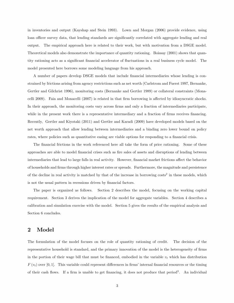
The temporary increase in borrowing cost along with the persistent decline in aggregate real activity
describes the U.S. experience (Graph 1) following the recent financial crisis. The spread between the three
month commercial paper and Treasury bill rates, a measure of firm borrowing cost, peaked at 1.4% in the
first quarter of 2009, but fell back to normal levels (below 0.2%) in the next quarter. In contrast, capacity
utilization and real GDP had made only a partial recovery a year later.
Results from VAR analysis confirm the relationships between aggregate and financial variables described
in the theoretical model. The survey of bank managers by the New York Federal Reserve provides an
empirical representation of credit market conditions, and capacity utilization is a proxy for the fraction
of firms receiving financing. The measure of tightness of credit markets according to the survey of bank
managers is negatively correlated with capacity utilization and real GDP for all specifications, while the role
of borrowing costs is not quantitatively significant, strong evidence for the importance of quantity rationing.
The role of quantity rationing has been emphasized in the literature from a number of different perspec-
tives. There is little empirical evidence for borrowing costs being important determinants of fluctuations
2
in inventories and output (Kayshap and Stein 1993). Lown and Morgan (2006) provide evidence, using
loan offi cer survey data, that lending standards are significantly correlated with aggregate lending and real
output. The empirical approach here is related to their work, but with motivation from a DSGE model.
Theoretical models also demonstrate the importance of quantity rationing. Boissay (2001) shows that quan-
tity rationing acts as a significant financial accelerator of fluctuations in a real business cycle model. The
model presented here borrows some modeling language from his approach.
A number of papers develop DSGE models that include financial intermediaries whose lending is con-
strained by frictions arising from agency restrictions such as net worth (Carlstrom and Fuerst 1997, Bernanke,
Gertler and Gilchrist 1996), monitoring costs (Bernanke and Gertler 1989) or collateral constraints (Mona-
celli 2009). Faia and Monacelli (2007) is related in that firm borrowing is affected by idiosyncratic shocks.
In their approach, the monitoring costs vary across firms and only a fraction of intermediaries participate,
while in the present work there is a representative intermediary and a fraction of firms receives financing.
Recently, Gertler and Kiyotaki (2011) and Gertler and Karadi (2009) have developed models based on the
net worth approach that allow lending between intermediaries and a binding zero lower bound on policy
rates, where policies such as quantitative easing are viable options for responding to a financial crisis.
The financial frictions in the work referenced here all take the form of price rationing. Some of these
approaches are able to model financial crises such as fire sales of assets and disruptions of lending between
intermediaries that lead to large falls in real activity. However, financial market frictions affect the behavior
of households and firms through higher interest rates or spreads. Furthermore, the magnitude and persistence
of the decline in real activity is matched by that of the increase in borrowing costs2 in these models, which
is not the usual pattern in recessions driven by financial factors.
The paper is organized as follows. Section 2 describes the model, focusing on the working capital
requirement. Section 3 derives the implication of the model for aggregate variables. Section 4 describes a
calibration and simulation exercise with the model. Section 5 gives the results of the empirical analysis and
Section 6 concludes.
2 Model
The formulation of the model focuses on the role of quantity rationing of credit. The decision of the
representative household is standard, and the primary innovation of the model is the heterogeneity of firms
in the portion of their wage bill that must be financed, embodied in the variable vt which has distribution
F (vt) over [0, 1]. This variable could represent differences in firms’internal financial resources or the timing
of their cash flows. If a firm is unable to get financing, it does not produce that period3 . An individual
3
firm with draw vt, has financing need φ (vt) = Wtl (vt) vt where Wt is the real wage, and l (vt) is the labor
demand for a producing firm. Firms are wage takers so Wt is the real wage for all firms. If the firm gets
financing, it produces output yt (vt) = atlt (vt)α where at is the level of productivity and the parameter α
takes values between zero and one.
Firms cannot commit to repayment of loans and so must provide collateral in the form of period t
output. The collateral condition is τ−1yt (vt) ≥ (1 + rt)φ (vt) where the real interest rate is rt and the
parameter τ−1 is the fraction of output the intermediary accepts as collateral. The productivity shock at
and need for financing vt are both realized at the beginning of period t, so the intermediary does not face
any uncertainty in the lending decision. Substituting for yt (vt) and φ (vt) yields the following form for the
collateral requirement.
τ−1atlt (vt)α ≥ (1 + rt)Wtlt (vt) vt (1)
The parameter τ represents the aggregate credit market stress embodied in the collateral requirements
made by banks and firms’ability to meet them. A sudden fall in confidence, i.e. a disturbance of animal
spirits, such as the collapse of the commercial paper market in the Fall of 2008, could be represented by an
exogenous rise4 in τ . Explicitly modeling changes in τ may be desirable, but the focus of the present paper
is to demonstrate the connection between credit market conditions and real economic activity.
Profit for an individual firm with realization vt for its financing need is the following.
Πt (vt) = atlt (vt)α −Wtlt (vt)− rtWtlt (vt) vt
Hence, labor demand for the firm is
αatlt (vt)α−1
=Wt (1 + rtvt) . (2)
Using the labor demand relation, the collateral constraint (1) becomes τ−1 (1 + rtvt) ≥ α (1 + rt) vt. From
this condition, we can define vt, the maximum vt above which firms cannot produce. For firms to produce
in period t, they must have a vt such that
vt ≤ vt = min{1, [τα (1 + rt)− rt]−1
}. (3)
Note that the fraction of firms producing vt is decreasing in the credit market stress parameter τ . At an
interior value for vt < 1, it must be the case that τα > 1, which implies that the fraction of firms producing
is decreasing in the interest rate.
4
Since the fraction of firms receiving financing vt is decreasing in the interest rate and does not respond
directly to other endogenous variables, it does not provide an accelerator mechanism for a shock to pro-
ductivity. This observation is a result of the particular form of equation (3). There are many alternative
specifications where labor demand or other endogenous quantities would enter, see Boissay (2001) for ex-
ample. Using such an alternative to model a financial accelerator mechanism is quite possible, but a full
investigation is left for future work.
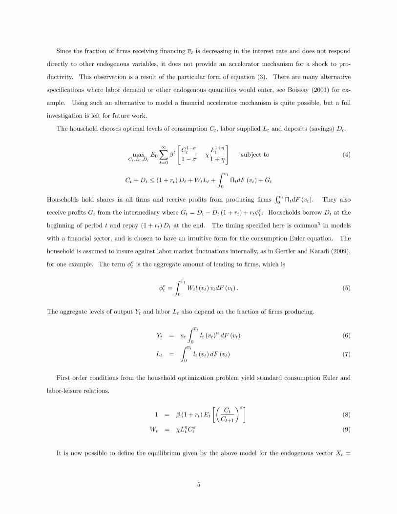
The household chooses optimal levels of consumption Ct, labor supplied Lt and deposits (savings) Dt.
maxCt,Lt,Dt
E0
∞∑t=0
βt
[C1−σt
1− σ − χL1+ηt
1 + η
]subject to (4)
Ct +Dt ≤ (1 + rt)Dt +WtLt +
∫ vt
0
ΠtdF (vt) +Gt
Households hold shares in all firms and receive profits from producing firms∫ vt0ΠtdF (vt). They also
receive profits Gt from the intermediary where Gt = Dt −Dt (1 + rt) + rtφet . Households borrow Dt at the
beginning of period t and repay (1 + rt)Dt at the end. The timing specified here is common5 in models
with a financial sector, and is chosen to have an intuitive form for the consumption Euler equation. The
household is assumed to insure against labor market fluctuations internally, as in Gertler and Karadi (2009),
for one example. The term φet is the aggregate amount of lending to firms, which is
φet =
∫ vt
0
Wtl (vt) vtdF (vt) . (5)
The aggregate levels of output Yt and labor Lt also depend on the fraction of firms producing.
Yt = at
∫ vt
0
lt (vt)αdF (vt) (6)
Lt =
∫ vt
0
lt (vt) dF (vt) (7)
First order conditions from the household optimization problem yield standard consumption Euler and
labor-leisure relations.
1 = β (1 + rt)Et
[(CtCt+1
)σ](8)
Wt = χLηtCσt (9)
It is now possible to define the equilibrium given by the above model for the endogenous vector Xt =
aggregate lending φet (5), aggregate labor (7), labor supply (9) and the consumption Euler equation (8). For
the goods market to clear, the relation Yt = Ct must hold. Also, deposits equal aggregate lending to firms
Dt = φet and financial intermediaries have zero profit in equilibrium Gt = 0. The above equations yield
steady state values X for a given level of productivity a, or a rational expectations equilibrium sequence
{Xt} for a specification of at.
3 Aggregate Output and Labor
The goal of this section is to establish the connection between aggregate output and the financial elements
of the model. For a fixed real wage, output is increasing in vt and decreasing in rt. When labor supply is
taken into account, the intuition is the same though some parameter restrictions are necessary. Propositions
about the response of steady state aggregate output are to changes in financial factors are given.
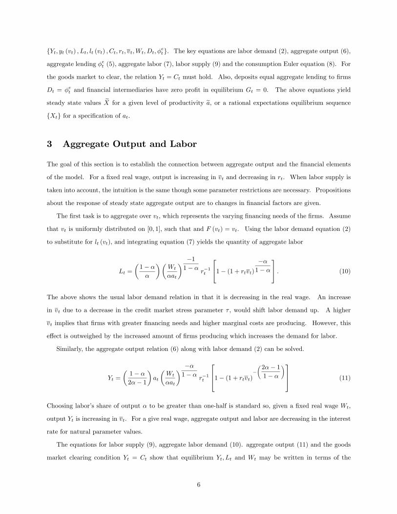
The first task is to aggregate over vt, which represents the varying financing needs of the firms. Assume
that vt is uniformly distributed on [0, 1], such that and F (vt) = vt. Using the labor demand equation (2)
to substitute for lt (vt), and integrating equation (7) yields the quantity of aggregate labor
Lt =
(1− αα
)(Wt
αat
) −11− α
r−1t
1− (1 + rtvt) −α1− α
. (10)
The above shows the usual labor demand relation in that it is decreasing in the real wage. An increase
in vt due to a decrease in the credit market stress parameter τ , would shift labor demand up. A higher
vt implies that firms with greater financing needs and higher marginal costs are producing. However, this
effect is outweighed by the increased amount of firms producing which increases the demand for labor.
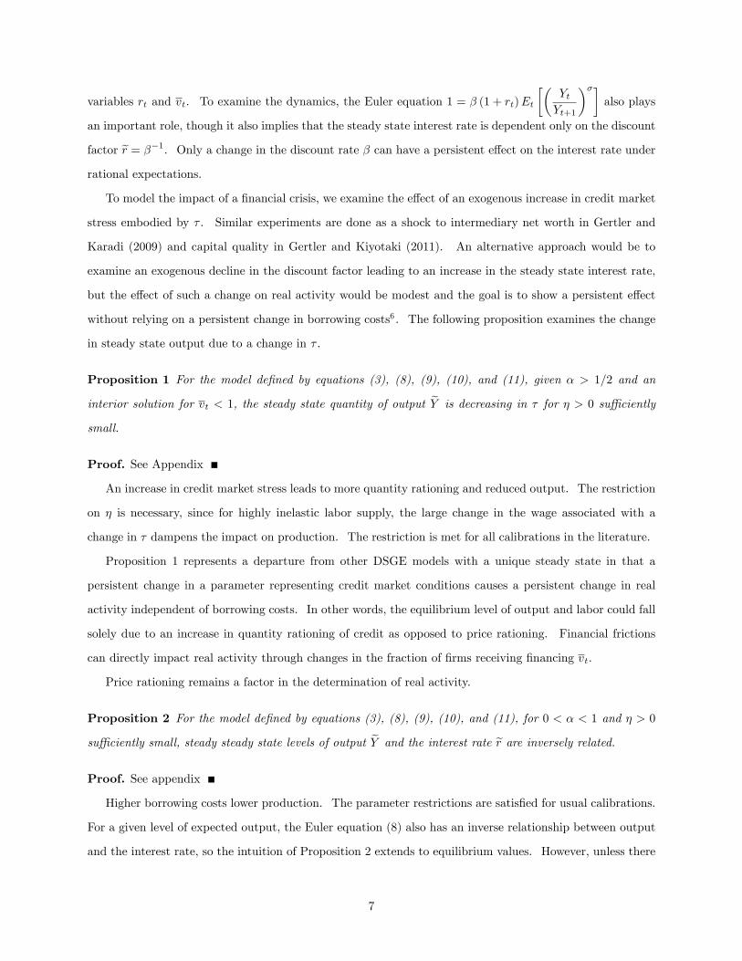
Similarly, the aggregate output relation (6) along with labor demand (2) can be solved.
Yt =
(1− α2α− 1
)at
(Wt
αat
) −α1− α
r−1t
1− (1 + rtvt)−(2α− 11− α
) (11)
Choosing labor’s share of output α to be greater than one-half is standard so, given a fixed real wage Wt,
output Yt is increasing in vt. For a give real wage, aggregate output and labor are decreasing in the interest
rate for natural parameter values.
The equations for labor supply (9), aggregate labor demand (10). aggregate output (11) and the goods
market clearing condition Yt = Ct show that equilibrium Yt, Lt and Wt may be written in terms of the
6
variables rt and vt. To examine the dynamics, the Euler equation 1 = β (1 + rt)Et
[(YtYt+1
)σ]also plays
an important role, though it also implies that the steady state interest rate is dependent only on the discount
factor r = β−1. Only a change in the discount rate β can have a persistent effect on the interest rate under
rational expectations.
To model the impact of a financial crisis, we examine the effect of an exogenous increase in credit market
stress embodied by τ . Similar experiments are done as a shock to intermediary net worth in Gertler and
Karadi (2009) and capital quality in Gertler and Kiyotaki (2011). An alternative approach would be to
examine an exogenous decline in the discount factor leading to an increase in the steady state interest rate,
but the effect of such a change on real activity would be modest and the goal is to show a persistent effect
without relying on a persistent change in borrowing costs6 . The following proposition examines the change
in steady state output due to a change in τ .
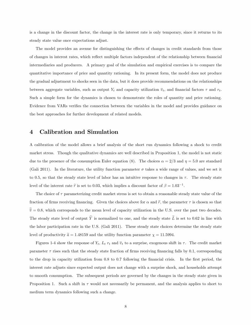
Proposition 1 For the model defined by equations (3), (8), (9), (10), and (11), given α > 1/2 and an
interior solution for vt < 1, the steady state quantity of output Y is decreasing in τ for η > 0 suffi ciently
small.
Proof. See Appendix
An increase in credit market stress leads to more quantity rationing and reduced output. The restriction
on η is necessary, since for highly inelastic labor supply, the large change in the wage associated with a
change in τ dampens the impact on production. The restriction is met for all calibrations in the literature.
Proposition 1 represents a departure from other DSGE models with a unique steady state in that a
persistent change in a parameter representing credit market conditions causes a persistent change in real
activity independent of borrowing costs. In other words, the equilibrium level of output and labor could fall
solely due to an increase in quantity rationing of credit as opposed to price rationing. Financial frictions
can directly impact real activity through changes in the fraction of firms receiving financing vt.
Price rationing remains a factor in the determination of real activity.
Proposition 2 For the model defined by equations (3), (8), (9), (10), and (11), for 0 < α < 1 and η > 0
suffi ciently small, steady steady state levels of output Y and the interest rate r are inversely related.
Proof. See appendix
Higher borrowing costs lower production. The parameter restrictions are satisfied for usual calibrations.
For a given level of expected output, the Euler equation (8) also has an inverse relationship between output
and the interest rate, so the intuition of Proposition 2 extends to equilibrium values. However, unless there
7
is a change in the discount factor, the change in the interest rate is only temporary, since it returns to its
steady state value once expectations adjust.
The model provides an avenue for distinguishing the effects of changes in credit standards from those
of changes in interest rates, which reflect multiple factors independent of the relationship between financial
intermediaries and producers. A primary goal of the simulation and empirical exercises is to compare the
quantitative importance of price and quantity rationing. In its present form, the model does not produce
the gradual adjustment to shocks seen in the data, but it does provide recommendations on the relationships
between aggregate variables, such as output Yt and capacity utilization vt, and financial factors τ and rt.
Such a simple form for the dynamics is chosen to demonstrate the roles of quantity and price rationing.
Evidence from VARs verifies the connection between the variables in the model and provides guidance on
the best approaches for further development of related models.
4 Calibration and Simulation
A calibration of the model allows a brief analysis of the short run dynamics following a shock to credit
market stress. Though the qualitative dynamics are well described in Proposition 1, the model is not static
due to the presence of the consumption Euler equation (8). The choices α = 2/3 and η = 5.0 are standard
(Gali 2011). In the literature, the utility function parameter σ takes a wide range of values, and we set it
to 0.5, so that the steady state level of labor has an intuitive response to changes in τ . The steady state
level of the interest rate r is set to 0.03, which implies a discount factor of β = 1.03−1.
The choice of τ parameterizing credit market stress is set to obtain a reasonable steady state value of the
fraction of firms receiving financing. Given the choices above for α and r, the parameter τ is chosen so that
v = 0.8, which corresponds to the mean level of capacity utilization in the U.S. over the past two decades.
The steady state level of output Y is normalized to one, and the steady state L is set to 0.62 in line with
the labor participation rate in the U.S. (Gali 2011). These steady state choices determine the steady state
level of productivity a = 1.48159 and the utility function parameter χ = 11.5994.
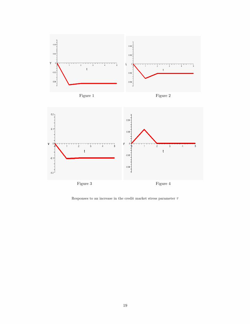
Figures 1-4 show the response of Yt, Lt rt and vt to a surprise, exogenous shift in τ . The credit market
parameter τ rises such that the steady state fraction of firms receiving financing falls by 0.1, corresponding
to the drop in capacity utilization from 0.8 to 0.7 following the financial crisis. In the first period, the
interest rate adjusts since expected output does not change with a surprise shock, and households attempt
to smooth consumption. The subsequent periods are governed by the changes in the steady state given in
Proposition 1. Such a shift in τ would not necessarily be permanent, and the analysis applies to short to
medium term dynamics following such a change.
8
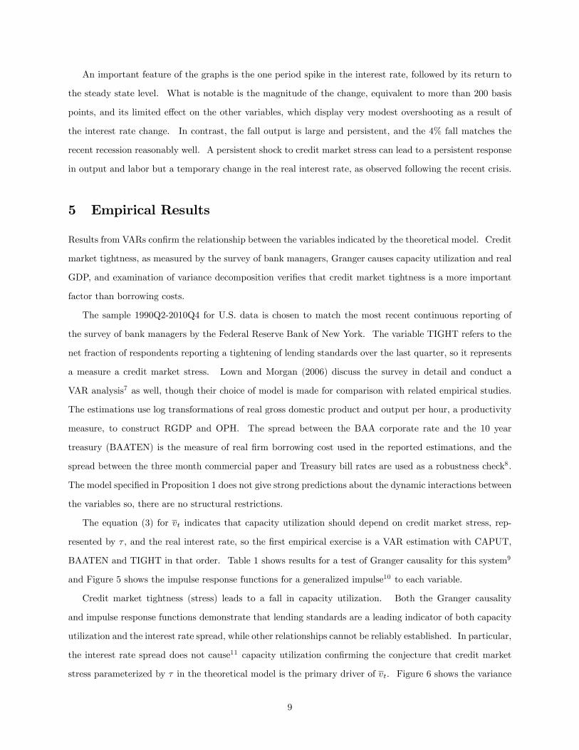
An important feature of the graphs is the one period spike in the interest rate, followed by its return to
the steady state level. What is notable is the magnitude of the change, equivalent to more than 200 basis
points, and its limited effect on the other variables, which display very modest overshooting as a result of
the interest rate change. In contrast, the fall output is large and persistent, and the 4% fall matches the
recent recession reasonably well. A persistent shock to credit market stress can lead to a persistent response
in output and labor but a temporary change in the real interest rate, as observed following the recent crisis.
5 Empirical Results
Results from VARs confirm the relationship between the variables indicated by the theoretical model. Credit
market tightness, as measured by the survey of bank managers, Granger causes capacity utilization and real
GDP, and examination of variance decomposition verifies that credit market tightness is a more important
factor than borrowing costs.
The sample 1990Q2-2010Q4 for U.S. data is chosen to match the most recent continuous reporting of
the survey of bank managers by the Federal Reserve Bank of New York. The variable TIGHT refers to the
net fraction of respondents reporting a tightening of lending standards over the last quarter, so it represents
a measure a credit market stress. Lown and Morgan (2006) discuss the survey in detail and conduct a
VAR analysis7 as well, though their choice of model is made for comparison with related empirical studies.
The estimations use log transformations of real gross domestic product and output per hour, a productivity
measure, to construct RGDP and OPH. The spread between the BAA corporate rate and the 10 year
treasury (BAATEN) is the measure of real firm borrowing cost used in the reported estimations, and the
spread between the three month commercial paper and Treasury bill rates are used as a robustness check8 .
The model specified in Proposition 1 does not give strong predictions about the dynamic interactions between
the variables so, there are no structural restrictions.
The equation (3) for vt indicates that capacity utilization should depend on credit market stress, rep-
resented by τ , and the real interest rate, so the first empirical exercise is a VAR estimation with CAPUT,
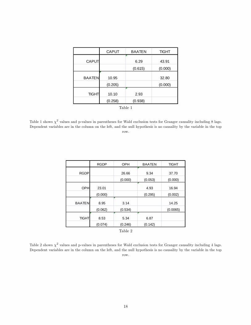
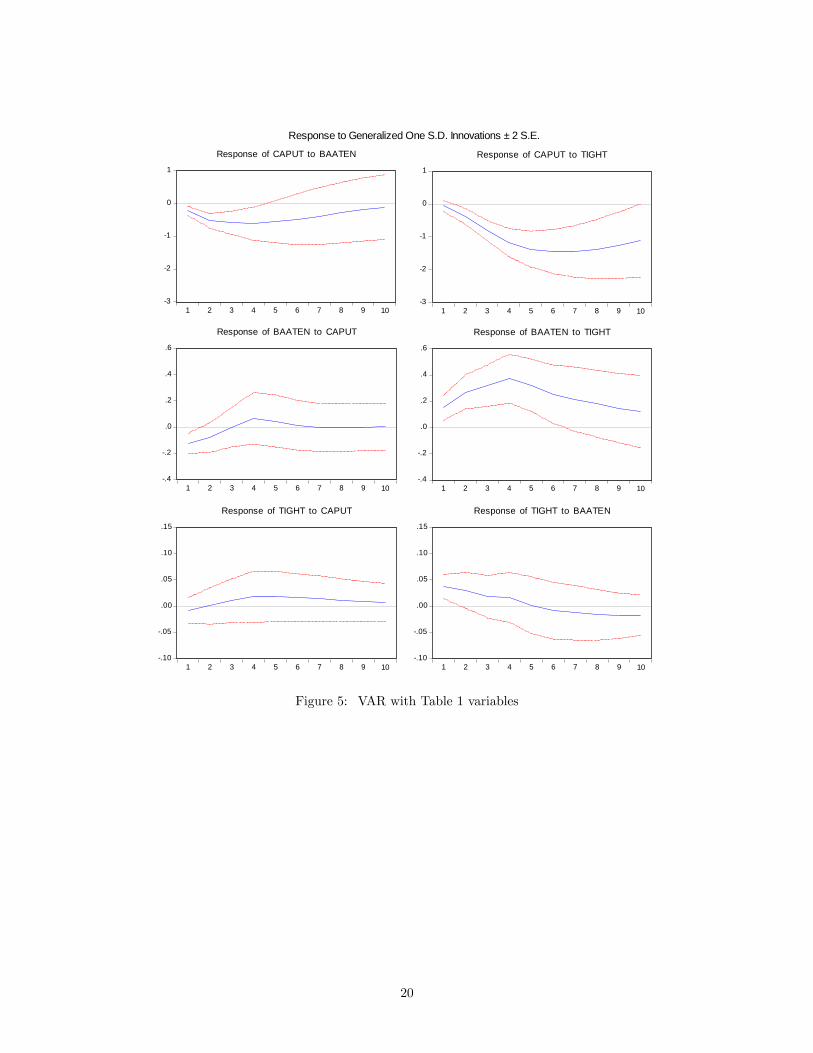
BAATEN and TIGHT in that order. Table 1 shows results for a test of Granger causality for this system9
and Figure 5 shows the impulse response functions for a generalized impulse10 to each variable.
Credit market tightness (stress) leads to a fall in capacity utilization. Both the Granger causality
and impulse response functions demonstrate that lending standards are a leading indicator of both capacity
utilization and the interest rate spread, while other relationships cannot be reliably established. In particular,
the interest rate spread does not cause11 capacity utilization confirming the conjecture that credit market
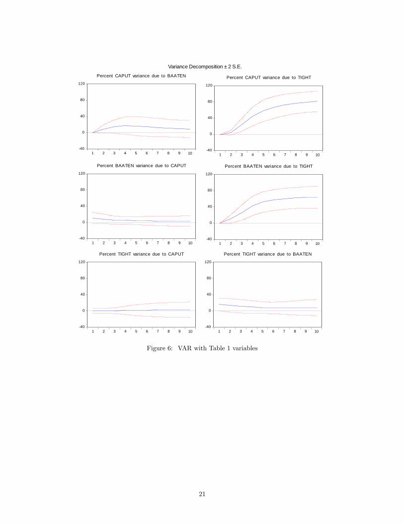
stress parameterized by τ in the theoretical model is the primary driver of vt. Figure 6 shows the variance
9
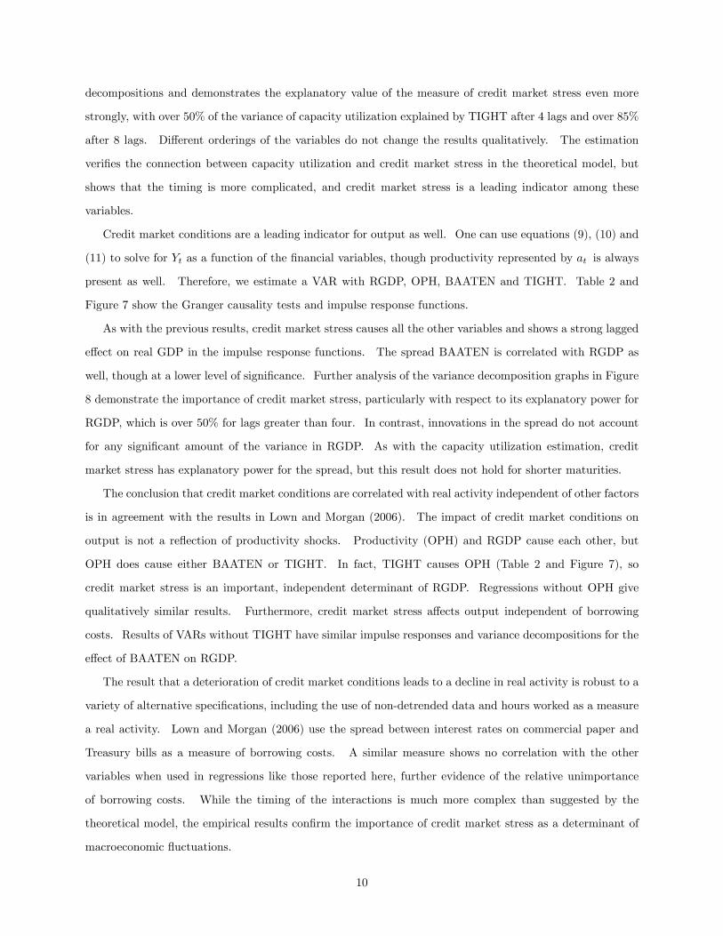
decompositions and demonstrates the explanatory value of the measure of credit market stress even more
strongly, with over 50% of the variance of capacity utilization explained by TIGHT after 4 lags and over 85%
after 8 lags. Different orderings of the variables do not change the results qualitatively. The estimation
verifies the connection between capacity utilization and credit market stress in the theoretical model, but
shows that the timing is more complicated, and credit market stress is a leading indicator among these
variables.
Credit market conditions are a leading indicator for output as well. One can use equations (9), (10) and
(11) to solve for Yt as a function of the financial variables, though productivity represented by at is always
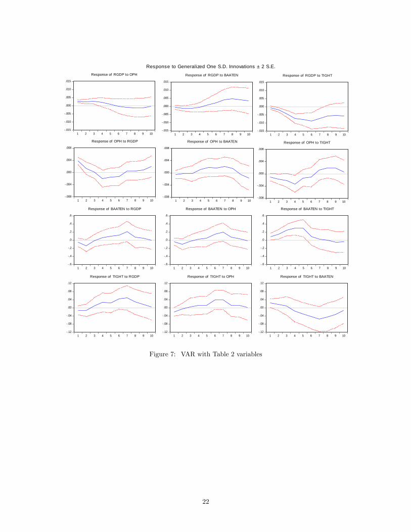
present as well. Therefore, we estimate a VAR with RGDP, OPH, BAATEN and TIGHT. Table 2 and
Figure 7 show the Granger causality tests and impulse response functions.
As with the previous results, credit market stress causes all the other variables and shows a strong lagged
effect on real GDP in the impulse response functions. The spread BAATEN is correlated with RGDP as
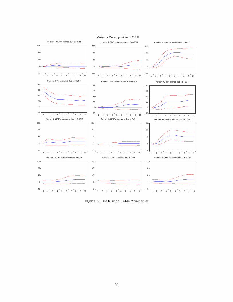
well, though at a lower level of significance. Further analysis of the variance decomposition graphs in Figure
8 demonstrate the importance of credit market stress, particularly with respect to its explanatory power for
RGDP, which is over 50% for lags greater than four. In contrast, innovations in the spread do not account
for any significant amount of the variance in RGDP. As with the capacity utilization estimation, credit
market stress has explanatory power for the spread, but this result does not hold for shorter maturities.
The conclusion that credit market conditions are correlated with real activity independent of other factors
is in agreement with the results in Lown and Morgan (2006). The impact of credit market conditions on
output is not a reflection of productivity shocks. Productivity (OPH) and RGDP cause each other, but
OPH does cause either BAATEN or TIGHT. In fact, TIGHT causes OPH (Table 2 and Figure 7), so
credit market stress is an important, independent determinant of RGDP. Regressions without OPH give
qualitatively similar results. Furthermore, credit market stress affects output independent of borrowing
costs. Results of VARs without TIGHT have similar impulse responses and variance decompositions for the
effect of BAATEN on RGDP.
The result that a deterioration of credit market conditions leads to a decline in real activity is robust to a
variety of alternative specifications, including the use of non-detrended data and hours worked as a measure
a real activity. Lown and Morgan (2006) use the spread between interest rates on commercial paper and
Treasury bills as a measure of borrowing costs. A similar measure shows no correlation with the other
variables when used in regressions like those reported here, further evidence of the relative unimportance
of borrowing costs. While the timing of the interactions is much more complex than suggested by the
theoretical model, the empirical results confirm the importance of credit market stress as a determinant of
macroeconomic fluctuations.
10
A question that arises in discussions of the impact of bank lending on GDP on other aggregate variables
is whether changes are driven by loan supply or demand. The results here suggest that loan supply is most
important, in agreement with Kayshap and Stein (1993) and Kayshap, Stein and Wilcox (1994). If output
and lending decline due to a demand shock such as a shock to business confidence, the interest rate would
be expected to fall with the demand for loans. However, the impulse responses in Figures 7 and 11 show
that a fall in RGDP is associated with a rise in the cost of borrowing to firms, and both are caused by a
tightening of lending standards. Furthermore, according the variance decomposition results in Figure 8,
RDGP does not have significant explanatory power with respect to BAATEN. Hence, a restriction in the
supply of loans is the most important financial factor to explain a decline in output.
6 Conclusion
The importance of financial frictions to macroeconomic fluctuations is undeniable, but the channel though
which they operate and the proper approach to modeling them are still diffi cult issues. While interest rates
and borrowing costs are important, there is evidence that they are not the primary factor. The present
paper offers a formal approach to quantity rationing of credit, where a loss of confidence on the part of
lenders or the inability of borrowers to provide collateral can lead to a denial of loans to some firms with a
direct impact on output and employment. While the role of the resulting fluctuations due to the interest
rate is temporary and small, quantity rationing can explain large changes in real activity.
Empirical analysis where the credit market stress is represented by data from the survey of bank managers
confirms the relationship between aggregate activity and financial variables described by the model. The
tightness of credit markets is a leading indicator of both capacity utilization and real GDP, while measures of
borrowing costs play a minor role. Since capacity utilization and real GDP have modest and inverse causal
impact (if any) on interest rate spreads, the VAR analysis provides evidence of the primary importance of
fluctuation in loan supply as opposed to demand.
There are many potential extensions of the present model. Besides the inclusion of more dynamic
elements, a more detailed description of the determinants of credit market conditions may also be desirable.
However, even in its present parsimonious form, the model demonstrates that quantity rationing of credit
provides a natural explanation for large aggregate fluctuations.
11
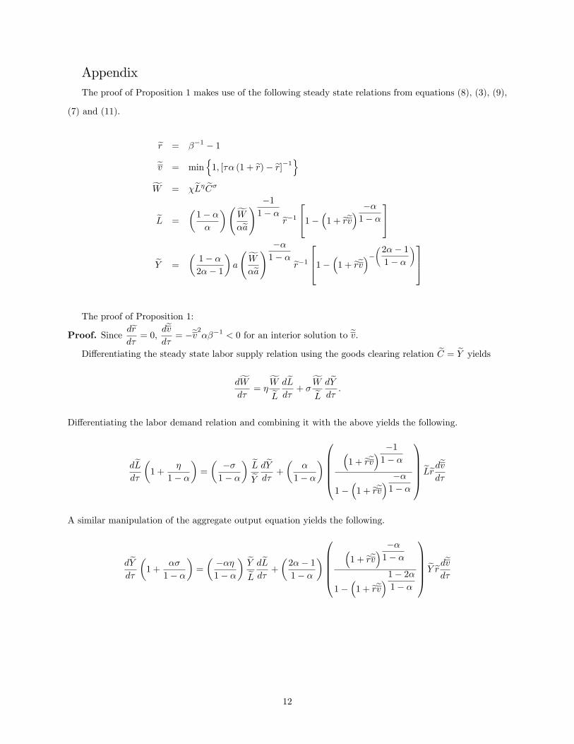
AppendixThe proof of Proposition 1 makes use of the following steady state relations from equations (8), (3), (9),
(7) and (11).
r = β−1 − 1
v = min{1, [τα (1 + r)− r]−1
}W = χLηCσ
L =
(1− αα
)(W
αa
) −11− α
r−1
1− (1 + rv) −α1− α
Y =
(1− α2α− 1
)a
(W
αa
) −α1− α
r−1
1− (1 + rv)−(2α− 11− α
)
The proof of Proposition 1:
Proof. Sincedr
dτ= 0,
dv
dτ= −v2αβ−1 < 0 for an interior solution to v.
Differentiating the steady state labor supply relation using the goods clearing relation C = Y yields
dW
dτ= η
W
L
dL
dτ+ σ
W
L
dY
dτ.
Differentiating the labor demand relation and combining it with the above yields the following.
dL
dτ
(1 +
η
1− α
)=
(−σ1− α
)L
Y
dY
dτ+
(α
1− α
)(1 + rv
) −11− α
1−(1 + rv
) −α1− α
Lrdv
dτ
A similar manipulation of the aggregate output equation yields the following.
dY
dτ
(1 +
ασ
1− α
)=
(−αη1− α
)Y
L
dL
dτ+
(2α− 11− α
)(1 + rv
) −α1− α
1−(1 + rv
)1− 2α1− α
Y rdv
dτ
12
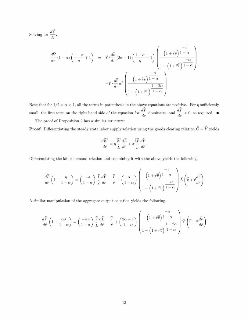
Solving fordY
dτ.
dY
dτ(1− α)
(1− αη
+ 1
)= Y r
dv
dτ(2α− 1)
(1− αη
+ 1
)(1 + rv
) −11− α
1−(1 + rv
) −α1− α
−Y r dvdτα2
(1 + rv
) −α1− α
1−(1 + rv
)1− 2α1− α
Note that for 1/2 < α < 1, all the terms in parenthesis in the above equations are positive. For η suffi ciently
small, the first term on the right hand side of the equation fordY
dτdominates, and
dY
dτ< 0, as required.
The proof of Proposition 2 has a similar structure:
Proof. Differentiating the steady state labor supply relation using the goods clearing relation C = Y yields
dW
dr= η
W
L
dL
dr+ σ
W
L
dY
dr.
Differentiating the labor demand relation and combining it with the above yields the following.
dL
dr
(1 +
η
1− α
)=
(−σ1− α
)L
Y
dY
dr− L
r+
(α
1− α
)(1 + rv
) −11− α
1−(1 + rv
) −α1− α
L
(v + r
dv
dr
)
A similar manipulation of the aggregate output equation yields the following.
dY
dr
(1 +
ασ
1− α
)=
(−αη1− α
)Y
L
dL
dr− Y
r+
(2α− 11− α
)(1 + rv
) −α1− α
1−(1 + rv
)1− 2α1− α
Y
(v + r
dv
dr
)
13
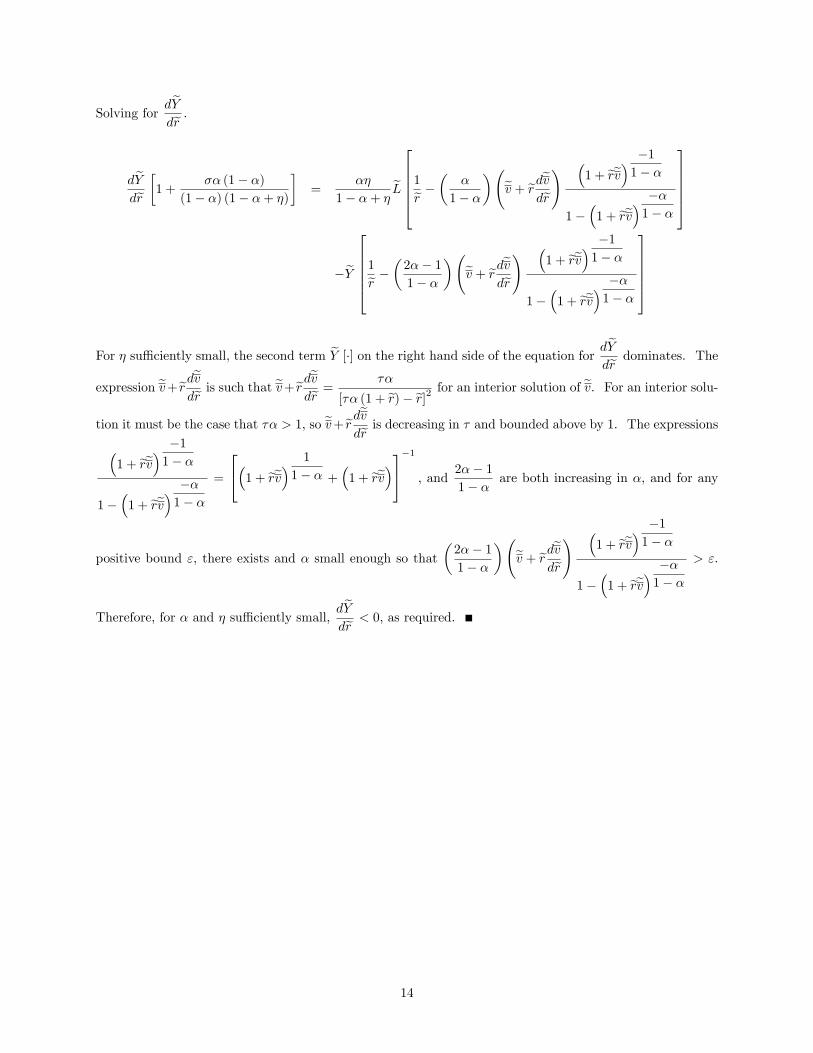
Solving fordY
dr.
dY
dr
[1 +
σα (1− α)(1− α) (1− α+ η)
]=
αη
1− α+ η L
1r −(
α
1− α
)(v + r
dv
dr
) (1 + rv
) −11− α
1−(1 + rv
) −α1− α
−Y
1r −(2α− 11− α
)(v + r
dv
dr
) (1 + rv
) −11− α
1−(1 + rv
) −α1− α
For η suffi ciently small, the second term Y [·] on the right hand side of the equation for dYdr
dominates. The
expression v+ rdv
dris such that v+ r
dv
dr=
τα
[τα (1 + r)− r]2for an interior solution of v. For an interior solu-
tion it must be the case that τα > 1, so v+ rdv
dris decreasing in τ and bounded above by 1. The expressions
(1 + rv
) −11− α
1−(1 + rv
) −α1− α
=
(1 + rv) 1
1− α +(1 + rv
)−1 , and 2α− 11− α are both increasing in α, and for any
positive bound ε, there exists and α small enough so that(2α− 11− α
)(v + r
dv
dr
) (1 + rv
) −11− α
1−(1 + rv
) −α1− α
> ε.
Therefore, for α and η suffi ciently small,dY
dr< 0, as required.
14
Notes
1Lown and Morgan (2006) have an extended section on the topic and quote Blanchard and Fisher (1989). Stiglitz and Weiss
(1981) give a theoretical basis for credit rationing, though for different reason than those in the present work.
2Kiyotaki and Moore (2008) is a related paper where liquidity shocks have a temporary effect on asset returns, though this
work is preliminary.
3A more realistic assumption would be that some firms or portions of firms always get financing. The present choice is
made for simplicity.
4Similarly, Gertler and Kiyotaki (2010) model the start of a crisis as a deterioration of the value of assets held by financial
intermediaries.
5For example, see Christiano and Eichenbaum (1992) and Ravenna and Walsh (2006).
6An increase in the the discount factor combined with the zero lower bound on the nominal interest rate can lead to a
substantial fall in output, see Christiano, Eichenbaum and Rebelo (2009).
7Jacobson, Linde and Roszbach (2005) also do an empirical analysis of the interaction between financial and macro variables
using VARs, among other techniques. They construct a measure of the frequency of bankruptcies for Sweden in the 1990s.
8Lown and Morgan use this spread at a maturity of six month, which is not available for the sample in the present work.
9The lag length criteria statistics recommend the use of one or two lags, but estimations of such systems have serially
correlated residuals so all the estimations reported here have 4 or 8 lags, appropriate for quarterly data.
10Except for the survey of bank managers all data available from the Federal Reserve Bank of St. Louis. The specification
for the generalized impulse responses, which are independent of the ordering of the variables, is due to Peseran and Shin (1989).
11 In this section, the word "causes" always refers to Granger causality.
References
Ben Bernanke and Mark Gertler (1989). "Agency Costs, Net Worth and Business Fluctuations." Amer-
ican Economic Review 79(1), 14-31.
Ben Bernanke, Mark Gertler and Simon Gilchrist (1996). "The Financial Accelerator in a Quantitative
Business Cycle Framework." in The Handbook of Macroeconomics 1(1), edited by John Taylor and Michael
Woodford, pp. 1341-1393, Elsevier, Amsterdam.
Olivier Blanchard and Stanley Fisher (1989). Lectures on Macroeconomics. Cambridge, MA.: MIT Press.
Federic Boissay (2001). "Credit Rationing, Output Gap, and Business Bycles." European Central Bank
Working Paper 87.
Charles Carlstrom and Timothy Fuerst (1997). "Agency Costs, Net Worth, and Business Fluctuations: A
Computable General Equilibrium Analysis," American Economic Review 87(5), 893-910.
Lawrence J. Christiano and Martin Eichenbaum (1992). "Liquidity Effects and the Monetary Transmission
15
Mechanism." American Economic Review 82(2), 346-353.
Lawrence J. Christiano, Martin Eichenbaum and Sergio Rebelo (2009). "When is the Government Spending
Multiplier Large." National Bureau of Economics Research Working Paper 15394.
Ester Faia and Tommaso Monacelli (2007). "Optimal Interest Rate Rules, Asset Prices, and Credit Fric-
tions." Journal of Economic Dynamics and Control 31(10), 3228-3254.
Jordi Gali (2011). "Monetary Policy and Unemployment." in The Handbook of Monetary Economics 3A,
edited by B. Friedman and M. Woodford pp. 487-546, Elsevier.
Mark Gertler and Peter Karadi (2009). "A Model of Unconventional Monetary Policy, manuscript.
Marik Gertler and Nobuhiro Kiyotaki (2011). "Financial Intermediation and Credit Policy in Business Cycle
Analysis, The Handbook of Macroeconomics (forthcoming), Elsevier, Amsterdam.
Tor Jacobson, Jesper Linde and Karl Roszbach (2004). "Exploring Interactions Between Real Activity and
the Financial Stance." Sveriges Riksbank Working Paper 184.
Cara Lown and Donald Morgan (2006). "The Credit Cycle and the Business Cycle: New Findings Using
the Loan Offi cer Opinion Survey." Journal of Money, Credit and Banking 38(6), 1574-1597.
Anil Kayshap and Jeremey Stein (1993). "Monetary Policy and Bank Lending." National Bureau of Eco-
nomics Research Working Paper 4317.
Anil Kayshap, Jeremey Stein and David Wilcox (1994). "Monetary Policy and Credit Conditions: Evidence
from the Composition of External Finance." American Economic Review 83(1) 78-98.
Nobuhiro Kiyotaki and John Moore (2008). "Liquidity, Business Cycles, and Monetary Policy." manuscript.
Tommaso Monacelli (2009). "New Keynesian Models, Durable Goods, and Collateral Constraints." Journal
of Monetary Economics 56, 242-254.
Hashem Peseran and Yongcheol Shin (1998). "Generalized Impulse Response Analysis in Linear Multivariate
Models, Economics Letters 58(1), 17-29.
Federico Ravenna and Carl Walsh (2006). "Optimal Monetary Policy with the Cost Channel." Journal of
Monetary Economics 53, 199-216.
16
Joseph Stiglitz and Andrew Weiss (1981). "Credit Rationing in Markets with Imperfect Information." Amer-
ican Economics Review 71(3) 393-410.
17
CAPUT BAATEN TIGHT
CAPUT 6.29 43.91
(0.615) (0.000)
BAATEN 10.95 32.80
(0.205) (0.000)
TIGHT 10.10 2.93
(0.258) (0.938)
Table 1
Table 1 shows χ2 values and p-values in parentheses for Wald exclusion tests for Granger causality including 8 lags.Dependent variables are in the column on the left, and the null hypothesis is no causality by the variable in the top
row.
RGDP OPH BAATEN TIGHT
RGDP 26.66 9.34 37.70
(0.000) (0.053) (0.000)
OPH 23.01 4.93 16.94
(0.000) (0.295) (0.002)
BAATEN 8.95 3.14 14.25
(0.062) (0.534) (0.0065)
TIGHT 8.53 5.34 6.87
(0.074) (0.246) (0.142)
Table 2
Table 2 shows χ2 values and p-values in parentheses for Wald exclusion tests for Granger causality including 4 lags.Dependent variables are in the column on the left, and the null hypothesis is no causality by the variable in the top
row.
18
Figure 1 Figure 2
Figure 3 Figure 4
Responses to an increase in the credit market stress parameter τ
19
3
2
1
0
1
1 2 3 4 5 6 7 8 9 10
Response of CAPUT to BAATEN
3
2
1
0
1
1 2 3 4 5 6 7 8 9 10
Response of CAPUT to TIGHT
.4
.2
.0
.2
.4
.6
1 2 3 4 5 6 7 8 9 10
Response of BAATEN to CAPUT
.4
.2
.0
.2
.4
.6
1 2 3 4 5 6 7 8 9 10
Response of BAATEN to TIGHT
.10
.05
.00
.05
.10
.15
1 2 3 4 5 6 7 8 9 10
Response of TIGHT to CAPUT
.10
.05
.00
.05
.10
.15
1 2 3 4 5 6 7 8 9 10
Response of TIGHT to BAATEN
Response to Generalized One S.D. Innovations ± 2 S.E.
Figure 5: VAR with Table 1 variables
20
40
0
40
80
120
1 2 3 4 5 6 7 8 9 10
Percent CAPUT variance due to BAATEN
40
0
40
80
120
1 2 3 4 5 6 7 8 9 10
Percent CAPUT variance due to TIGHT
40
0
40
80
120
1 2 3 4 5 6 7 8 9 10
Percent BAATEN variance due to CAPUT
40
0
40
80
120
1 2 3 4 5 6 7 8 9 10
Percent BAATEN variance due to TIGHT
40
0
40
80
120
1 2 3 4 5 6 7 8 9 10
Percent TIGHT variance due to CAPUT
40
0
40
80
120
1 2 3 4 5 6 7 8 9 10
Percent TIGHT variance due to BAATEN
Variance Decomposition ± 2 S.E.
Figure 6: VAR with Table 1 variables
21
.015
.010
.005
.000
.005
.010
.015
1 2 3 4 5 6 7 8 9 10
Response of RGDP to OPH
.015
.010
.005
.000
.005
.010
.015
1 2 3 4 5 6 7 8 9 10
Response of RGDP to BAATEN
.015
.010
.005
.000
.005
.010
.015
1 2 3 4 5 6 7 8 9 10
Response of RGDP to TIGHT
.008
.004
.000
.004
.008
1 2 3 4 5 6 7 8 9 10
Response of OPH to RGDP
.008
.004
.000
.004
.008
1 2 3 4 5 6 7 8 9 10
Response of OPH to BAATEN
.008
.004
.000
.004
.008
1 2 3 4 5 6 7 8 9 10
Response of OPH to TIGHT
.6
.4
.2
.0
.2
.4
.6
1 2 3 4 5 6 7 8 9 10
Response of BAATEN to RGDP
.6
.4
.2
.0
.2
.4
.6
1 2 3 4 5 6 7 8 9 10
Response of BAATEN to OPH
.6
.4
.2
.0
.2
.4
.6
1 2 3 4 5 6 7 8 9 10
Response of BAATEN to TIGHT
.12
.08
.04
.00
.04
.08
.12
1 2 3 4 5 6 7 8 9 10
Response of TIGHT to RGDP
.12
.08
.04
.00
.04
.08
.12
1 2 3 4 5 6 7 8 9 10
Response of TIGHT to OPH
.12
.08
.04
.00
.04
.08
.12
1 2 3 4 5 6 7 8 9 10
Response of TIGHT to BAATEN
Response to Generalized One S.D. Innovations ± 2 S.E.