Quantization, sampling theorem & DAC

"The Scientist and Engineer's Guide to Digital Signal

Processing, copyright ©1997-1998 by Steven W. Smith."

Quantization, sampling

theorem & DAC

Claudia Feregrino-Uribe & Alicia Morales-Reyes

Original material: Rene Cumplido

Autumn 2015, CCC-INAOE



Contents

• Quantization • The Sampling Theorem • Digital to Analog Conversion



Quantization



Most of the signals directly encountered in science and engineering are continuous Analog-to-Digital Conversion (ADC) and Digital-to-Analog Conversion (DAC) are the processes that allow digital computers to interact with these everyday signals.

Introduction



Digital information is different from its continuous counterpart in two important respects:

It is sampled, and it is quantized. Both of these restrict how much information a digital signal can contain.

Introduction



The next figure is an analog signal to be digitized.

Example

This signal is a voltage that varies over time. We will assume that the voltage can vary from 0 to 4.095 volts, that will be produced by a 12 bit digitizer



Sampling converts the independent variable (time in this example) from continuous to discrete.

Example The conversion is broken into two stages to allow the effects of sampling to be separated from the effects of quantization.



The first stage is the sample-and-hold (S/H), where the only information retained is the instantaneous value of the signal when the periodic sampling takes place.

Sample and Hold



In the second stage, the ADC converts the voltage to the nearest integer number. This results in each sample in the digitized signal having an error of up to ±½ LSB.

ADC



Quantization Sampled analog signal Digitized signal

In most cases, quantization results in nothing more than the

addition of a specific amount of random noise to the signal.

Quantization The additive noise is uniformly distributed between ±½ LSB, has a mean

of zero, and a standard deviation of LSB 1/√12 (-0.29 LSB)

For example, passing an analog signal through an 8 bit digitizer adds an rms noise of: 0.29/256, or about 1/900 of the full scale value

A 12 bit conversion adds a noise of: 0.29 /4096 ≈ 1 /14,000

A 16 bit. conversion adds: 0.29/65536 ≈ 1 /227,000

Since quantization error is a random noise, the number of bits determines the precision of the data.

The statement: "We increased the precision of the measurement from 8 to 12 bits.“ is correct in this case.



Since quantization error is a random noise, the number of bits determines the precision of the data. For example, imagine an analog signal with a maximum amplitude of 1.0 volt, and a random noise of 1.0 millivolt rms. Digitizing this signal to 8 bits results in 1.0 volt becoming digital number 255, and 1.0 millivolt becoming 0.255 LSB

Quantization



Random noise signals are combined by adding their variances. That is, the signals are added in quadrature:

The total noise on the digitized signal is therefore given by This is an increase of about 50% over the noise already in the analog signal.

Quantization



Digitizing this same signal to 12 bits would produce virtually no increase in the noise, and nothing would be lost due to quantization.

When faced with the decision of how many bits are needed in a system, ask two questions: (1)How much noise is already present in the analog signal? (1)How much noise can be tolerated in the digital signal?

Quantization



When isn't this model of quantization valid?

Only when the quantization error cannot be treated as random. The

only common occurrence of this is when the analog signal remains at

about the same value for many consecutive samples.

The quantization error now looks like a thresholding effect

Quantization

The Figure shows how an analog

signal that varies less than ±½

LSB can become stuck on the

same quantization level during

digitization.



The Sampling Theorem



The definition of proper sampling is quite simple. Suppose you sample a continuous signal in some manner. If you can exactly reconstruct the analog signal from the samples, you must have done the sampling properly. Even if the sampled data appears confusing or incomplete, the key information has been captured if you can reverse the process.

Proper Sampling



A continuous signal is sampled properly if the samples contain all the information needed to recreated the original waveform.

Proper Sampling



Example (1)

The continious line represents the analog signal entering the ADC, while the square markers are the digital signal leaving the ADC The analog signal is a constant DC value, a cosine wave of zero frequency All of the information needed to reconstruct the analog signal is contained in the digital data. This is proper sampling.



Example (2)

This situation is more complicated than the previous case, because the analog signal cannot be reconstructed by simply drawing straight lines between the data points. The sine wave has a frequency of 0.09 of the sampling rate.

E.g. a 90 cycle/second sine wave being sampled at 1000 sps

There are 11.1 samples taken over each complete cycle of the sinusoid.

Do these samples properly represent the analog signal?



Example (2)

The answer is yes, because no other sinusoid, or combination of sinusoids, will produce this pattern of samples. These samples correspond to only one analog signal, and therefore the analog signal can be exactly reconstructed. Again, an instance of proper sampling.



Example (3)

Now, the situation is made more difficult by increasing the sine wave's frequency to 0.31 of the sampling rate. This results in only 3.2 samples per sine wave cycle. Do these samples properly represent the analog waveform?



Example (3)

Again, the answer is yes, and for exactly the same reason. The samples are a unique representation of the analog signal. All of the information needed to reconstruct the continuous waveform is contained in the digital data. Obviously, it must be more sophisticated than just drawing straight lines between the data points. This is still proper sampling according to our definition.



Example (4)

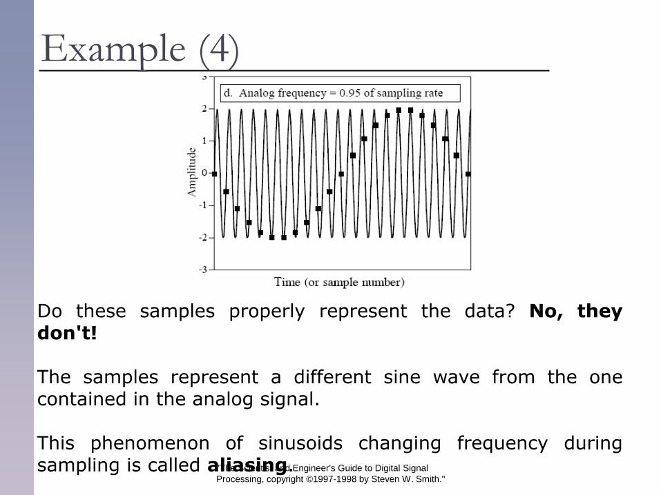
Do these samples properly represent the data? No, they don't! The samples represent a different sine wave from the one contained in the analog signal. This phenomenon of sinusoids changing frequency during sampling is called aliasing.



The Sampling Theorem Frequently this is called the Shannon sampling theorem, or the Nyquist sampling theorem.

The sampling theorem indicates that a continuous signal can be properly sampled, only if it does not contain frequency components above one-half of the sampling rate.




For instance, a sampling rate of 200 samples/second requires the analog signal to be composed of frequencies below 100 cycles/second. If frequencies above this limit are present in the signal, they will be aliased to frequencies between 0 and 100 cycles/second.




The figure shows how frequencies are changed during aliasing. The key point to remember is that a digital signal cannot contain frequencies above one-half the sampling rate (i.e.,

the Nyquist frequency/rate).



The Sampling Theorem The last Figure shows the conversion of analog frequency into digital frequency during sampling. Continuous signals with a frequency less than one-half of the sampling rate are directly converted into the corresponding digital frequency. Above one-half of the sampling rate, aliasing takes place, resulting in the frequency being misrepresented in the digital data. Aliasing always changes a higher frequency into a lower frequency between 0 and 0.5. In addition, aliasing may also change the phase of the signal by 180 degrees.



The Sampling Theorem Now we will dive into a more detailed analysis of sampling and how aliasing occurs. Our overall goal is to understand what happens to the information when a signal is converted from a continuous to a discrete form. The problem is, these are very different things; one is a continuous waveform while the other is an array of numbers.



The Sampling Theorem Figure shows the signal sampled by using an impulse train. The impulse train is a continuous signal consisting of a series of narrow spikes (impulses) that match the original signal at the sampling instants.




Keep in mind that the impulse train is a theoretical concept, not a waveform that can exist in an electronic circuit. In terms of information content, they are identical. If one is known, it is trivial to calculate the other.



The Sampling Theorem Analog signal we wish to sample As indicated by its frequency spectrum, it is composed only of frequency components between 0 and about 0.33 fs. (fs = sampling frequency)

For example, this might be a speech signal that has been filtered to

remove all frequencies above 3.3 kHz. Correspondingly, fs would be 10 kHz

(10,000 samples/second)



The Sampling Theorem Sampling the last signal in by using an impulse train produces the signal shown below. Each multiple of the sampling frequency, fs, 2fs, 3fs, 4fs, etc., has received a copy and a left-forright flipped copy of the original frequency spectrum.



The Sampling Theorem Sampling has generated new frequencies. Is this proper sampling? The answer is yes, because the sampling signal can be transformed back into the original signal by eliminating all frequencies above ½fs.



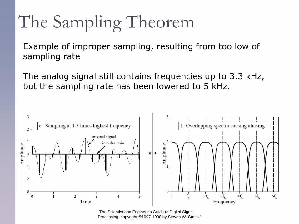
The Sampling Theorem Example of improper sampling, resulting from too low of sampling rate The analog signal still contains frequencies up to 3.3 kHz, but the sampling rate has been lowered to 5 kHz.



The Sampling Theorem Since there is no way to separate the overlapping frequencies, information is lost, and the original signal cannot be reconstructed. This overlap occurs when the analog signal contains frequencies greater than one-half the sampling rate, that is, we have proven the sampling theorem.



Digital-to-Analog Conversion




In theory, the simplest method for digital-to-analog conversion is to pull the samples from memory and convert them into an impulse train.




The original signal and the impulse train have identical frequency spectra below the Nyquist frequency (one-half the sampling rate). At higher frequencies, the impulse train contains a duplication of this information, while the original analog signal contains nothing (assuming aliasing did not occur).




All DACs operate by holding the last value until another sample is received. This is called a zeroth-order hold, the DAC equivalent of the sample-and-hold used during ADC. The zeroth-order hold produces the staircase appearance shown in the next figure




In the frequency domain, the zeroth-order hold results in the spectrum of the impulse train being multiplied by the dark curve shown in the last figure, given by the equation:

This is of the general form: ,called the sinc function or sinc(x).




The light line shows the frequency spectrum of the impulse train (the "correct“ spectrum) The dark line shows the sinc The frequency spectrum of the zeroth order hold signal is equal to the product of these two curves.




The analog filter used to convert the zeroth-order hold

signal, into the reconstructed signal, needs to do two things:

(1)remove all frequencies above one-half of the sampling rate.

(2)Boost the frequencies by the reciprocal of the zeroth-order hold's effect, i.e., 1/sinc(x)




Before leaving this section on sampling, we need to dispel a common myth about analog versus digital signals.

"Since analog signals use continuous parameters, they have infinitely good resolution in both the independent and the dependent variables.“

True or False?




Not true! Analog signals are limited by the same two problems as digital signals: noise and bandwidth. The noise in an analog signal limits the measurement of the waveform's amplitude, just as quantization noise does in a digital signal. Likewise, the ability to separate closely spaced events in an analog signal depends on the highest frequency allowed in the waveform.




For instance, an analog signal formed from frequencies between DC and 10 kHz will have exactly the same resolution as a digital signal sampled at 20 kHz. It must, since the sampling theorem guarantees that the two contain the same information.



Dithering is a common technique for improving the digitization of these slowly varying signals.

Dithering

Dithering improves this situation by

adding a small amount of random

noise to the analog signal.

In this example, the added noise is

normally distributed with a standard

deviation of 2/3 LSB.



After digitization, the computer can subtract the random numbers from the digital signal using floating point arithmetic. This technique is called subtractive dither, but is only used in the most elaborate systems. The simplest method, although not always possible, is to use the noise already present in the analog signal for dithering.

Dithering

Date post:	23-Feb-2022
Category:	Documents
Upload:	others
View:	12 times
Download:	0 times

Quantization, sampling theorem & DAC

Documents