Quanto Interest-Rate Exchange Options in a Cross-Currency LIBOR Market Model Tsung-Yu Hsieh (Department of Banking and Finance, Tamkang University, Taiwan) Chi-Hsun Chou (Department of Management, Fo Guang University, Taiwan) Ting-Pin Wu (Department of Finance, National Central University, Taiwan) Son-Nan Chen (Shanghai Advanced Institute of Finance, Shanghai Jiao Tong University) Abstract The purpose of this paper is to price quanto interest-rate exchange options (QIREOs) based on a practical and easy-to-use interest-rate model. A new model, namely the cross-currency LIBOR market model, is used to extend the initial LIBOR market model from a single-currency economy to a cross-currency economy. The cross-currency LIBOR market model is suitable and applicable to pricing a variety of quanto-type interest-rate derivatives. Four different types of quanto interest-rate exchange options are priced in this article. Hedging strategies and calibration procedures are also examined in detail for practical implementation. Furthermore, Monte-Carlo simulation is provided to evaluate the accuracy of the theoretical prices. Key words: Quanto Interest-Rate Exchange Options, Cross-Currency LIBOR Market Model.
Transcript
Quanto Interest-Rate Exchange Options
in a Cross-Currency LIBOR Market Model
Tsung-Yu Hsieh (Department of Banking and Finance, Tamkang University, Taiwan)
Chi-Hsun Chou (Department of Management, Fo Guang University, Taiwan)
Ting-Pin Wu (Department of Finance, National Central University, Taiwan)
Son-Nan Chen (Shanghai Advanced Institute of Finance, Shanghai Jiao Tong University)
Abstract
The purpose of this paper is to price quanto interest-rate exchange options (QIREOs)
based on a practical and easy-to-use interest-rate model. A new model, namely the
cross-currency LIBOR market model, is used to extend the initial LIBOR market model from
a single-currency economy to a cross-currency economy. The cross-currency LIBOR market
model is suitable and applicable to pricing a variety of quanto-type interest-rate derivatives.
Four different types of quanto interest-rate exchange options are priced in this article.
Hedging strategies and calibration procedures are also examined in detail for practical
implementation. Furthermore, Monte-Carlo simulation is provided to evaluate the accuracy of
the theoretical prices.
Key words: Quanto Interest-Rate Exchange Options, Cross-Currency LIBOR Market Model.
1
1. Introduction
Quanto interest-rate exchange options (QIREOs), also known as interest-rate difference
options, are options written on the difference between two interest rates that are available in
different currencies or between two interest rates in one currency, with the final payments
made in domestic currency. Interest rate volatility during the past decade has magnified the
risk due to an unfavorable shift in the term structure of interest rates, thereby leading to a
dramatic increase in the number and types of contingent claims that incorporate options on
change in the level of interest rates. These products have been developed to enhance the
ability of asset/liability managers to alter their interest-rate exposure. As a result, QIREOs are
evolved to exploit interest-rate differentials without directly incurring exchange-rate risk.
The applications of QIREOs are quite extensive and similar to those of differential swaps.
However, QIREOs provide more flexibility in certain applications. First, QIREOs provide a
mechanism for achieving a payoff based on the differential of interest rates available in two
different currencies, which is not directly affected by movements in exchanges rates. Second,
as compared with differential swaps, the major advantage of QIREOs is that they can be used
to fit a very specific strategy since they can be tailored to provide payoffs that depend on
whether the spread of two interest rates is above or below a specified level, or within or
outside a specified range on a specific date in the future. Third, QIREOs can provide added
precision to a strategy involving differential swaps. For example, a portfolio manager might
use a differential swap to capitalize on anticipated yield-curve movements while also
purchasing an QIREO on the spread in order to limit his downside risk. Moreover, money
market investors may use QIREOs to take advantage of a high-yield currency; asset managers
may adopt QIREOs to enhance their portfolio return; liability managers and other borrowers
can employ QIREOs to reduce their effective borrowing rates.
Despite the wide applications of QIREOs, the academic literature has paid little attention
to how to price such options, especially in the framework of the LIBOR market model.
Therefore, the purpose of this article is to price QIREOs based on a practical and easy-to-use
interest rate model. In addition, it is worth noting that the well-known “quanto-effect” has to
be considered as dealing with foreign assets paid in domestic currency. To achieve this aim, a
new model, namely the cross-currency LIBOR market model, is introduced to extend the
initial LIBOR market model from a single-currency economy to a cross-currency economy
and then adopted to price QIREOs.
2
This paper employs the cross-currency LIBOR market model to price QIREOs for the
following merits. Those interest-rate models that have been developed for pricing
interest-rate derivatives can be, loosely speaking, divided into two types: traditional
interest-rate models and market models. The traditional interest-rate models, such as the
Vasicek model, the Cox-Ingersoll-Ross (CIR) model and the Heath-Jarrow-Morton (HJM)
model, describe the behavior of interest rates by specifying market-unobservable and abstract
interest rates, such as instantaneous short and forward rates. Contrarily, the LIBOR and swap
market models are constructed by specifying market-observable LIBOR and swap rates.
There are some drawbacks to the traditional models. First, because of their abstract and
market-unobservable short and forward rates, the underlying market rates, such as LIBOR
and swap rates, have to be obtained through a complicated transformation of the abstract rates.
Second, the compounding period of their underlying rate is infinitesimal, which contradicts
with the market convention of being discretely compounded. Third, caps (floors) and
swaptions are the most important and popular interest-rate products that are actively traded
in financial markets. The pricing formulae derived from the traditional interest-rate models
are incompatible with the widely used Black’s formula. As a result, the model calibration
procedure is rendered difficulty to execute efficiently. Moreover, most of the traditional
models are Gaussian term structure models. As examined in Rogers (1996), Gaussian term
structure models have an important theoretical limitation: the rates can attain negative values
with positive probability, a tendency which in many cases may cause some pricing errors. In
order to improve the aforementioned drawbacks, a new approach to modelling interest-rate
behavior has been developed. It is the LIBOR market model (LMM).
The LMM has been developed by Musiela and Rutkowski (1997), Miltersen, Sandmann
and Sondermann (1997), and Brace, Gatarek and Musiela (1997, BGM). Because of the
following advantages, the model is widely adopted by practitioners. First, the rates modeled
are the LIBOR rates, which are market-observable and consistent with the market convention
of being discretely compounded. Second, the cap and floor pricing formulae follow the
Black’s formula, which is consistent with market practice and makes the calibration
procedure easier. Moreover, BGM have shown that under the forward measures forward
LIBOR rates have a lognormal volatility structure that prevents the forward LIBOR rates
from becoming negative with a positive probability. As a result, pricing errors arising from
negative rates are avoided.
3
Furthermore, Wu and Chen (2007) have extended the original BGM model from a
single-currency economy to a cross-currency case. They have also incorporated the exchange
rate process into the general model setting. Their cross-currency LIBOR market model is
very general. Thus, it is suitable to use this model for pricing quanto-type interest-rate
derivatives that depend on domestic and foreign interest rates. As a result, the cross-currency
LMM will be employed in this article to price four different types of QIREOs.
The remainder of this article is organized as follows. Section 2 briefly describes the
development and the framework of the cross-currency LIBOR market model, which is
directly drawn from Wu and Chen (2007). Section 3 derives the pricing formulae of the four
different types of QIREOs based on the cross-currency BGM (LMM) model. The hedging
strategy of each option is also examined. Section 4 provides the calibration procedure for
practical implementation and examines the accuracy of the pricing formulae via Monte-Carlo
simulation. Section 5 concludes the paper with a brief summary.
2. The Arbitrage-Free Cross-Currency HJM Model and the Arbitrage-Free
Cross-Currency BGM Model
In this section, we briefly describe the development and the framework of the
cross-currency LIBOR market model as derived by Wu and Chen (2007). Subsection 2.1
establishes an arbitrage-free cross-currency HJM model.1 Under the arbitrage-free
relationship between the drift and the volatility terms in the cross-currency HJM model, an
arbitrage-free cross-currency BGM model is also introduced in Subsection 2.2.
2.1 Arbitrage-Free Cross-Currency HJM Model
Assume that trading takes place continuously in time over an interval 0, ,0 .
The uncertainty is described by the filtered probability space 0,, , ,
tF P F
where the
filtration is generated by independent standard Brownian motions
1 2, ,..., mW t W t W t W t . P represents the actual probability measure. The notations
are given below with d for domestic and f for foreign:
,kf t T = the kth country’s forward interest rate contracted at time t for instantaneous
borrowing and lending at time T with 0 t T , where ,k d f .
,kP t T = the time t price of the kth country’s zero coupon bond (ZCB) paying one dollar
at time T.
4
kr t = the kth country’s risk-free short rate at time t.
k t = 0
expt
kr u du , the kth country’s money market account at time t with an
initial value 0 1k .
X t = the spot exchange rate at 0,t for one unit of foreign currency expressed
in terms of domestic currency.
Assumption 2.1 A FAMILY OF FORWARD RATE PROCESS
For any given 0,T , the dynamics of the forward rate ,kf t T , ,k d f , follows
the following process:
, , , , 0k fk fkdf t T t T dt t T dW t t T , (2.1)
where 0, : 0,kf T T is a nonrandom initial forward curve, ,fk t T and
1, , ,..., ,fk fk fkmt T t T t T satisfy some regular conditions.2
Equation (2.1) is the notable HJM interest-rate model. Through the various specifications
for the volatility coefficients, the random shocks generate significantly different qualitative
characteristics of the forward rate processes.
The Zero-Coupon bond price (ZCB) ,kP t T , ,k d f , is defined as:
, exp ,T
k ktP t T f t u du . (2.2)
From (2.1) and (2.2), the dynamics of the ZCB price can be derived as given below
,, , , 0
,k
k k Pkk
dP t Tr t b t T dt t T dW t t T
P t T , (2.3)
where 1, , ,..., ,Pk Pk Pkmt T t T t T with
2, , 1,2,...,T
Pki fkitt T t u du for i m
and 21, , ,2
T
k fk Pktb t T t u du t T .
Assumption 2.2 THE SPOT EXCHANGE RATE DYNAMICS
The dynamics of the spot exchange rate X t is given as follows:
X XdX t X t t dt X t t dW t , (2.4)
where X t and 1, ,...,X X Xmt T t t satisfy some regular conditions.3
5
For greater flexibility, the number of the random shocks, m, are not designated exactly.
Rather, they are stipulated dependent on the simplicity and accuracy required by the user. For
example, six random shocks may be used to capture all factors causing the stochastic
behaviors of the entire forward rate curve and the spot exchange rate. The first two random
shocks can be interpreted, respectively, as the short-term and the long-term factors causing
the shift of different maturity ranges on the domestic term structure. Similarly, the third and
fourth shocks have the same effects on the foreign case. The correlation between the domestic
and the foreign term structure is affected by the fifth shock. The remaining shock can be
interpreted as the factor that causes unanticipated movements in the exchange rate.
In order to make the economy both complete and arbitrage (i.e., there exists a unique
martingale measure4), some conditions are imposed upon the previous dynamics. Under these
conditions, the volatility terms of all the stochastic processes remain unchanged, but the drift
terms become some special structures. These corresponding relationships between the drift
and the volatility terms will be employed in the next section to derive the cross-currency
LIBOR market model.
To determine the unique domestic martingale measure,5 all assets must be denominated in
domestic currency. Therefore, the foreign assets must be denominated in domestic currency
and regarded as the ‘general’ domestic assets. Define * , ,f fP t T P t T X t ,
* ,f ft T t X t . Then, all the domestic-currency-denominated assets are discounted by
the domestic money market account and listed as follows:
,
, dPd
d
P t TZ t T
t ,
* ,, f
Pfd
P t TZ t T
t ,
* ,, f
rfd
t TZ t T
t
.
By Ito’s lemma, the stochastic processes of these domestic-currency-denominated assets
can be expressed as follows:
,, ,
,Pd
d PdPd
dZ t Tb t T dt t T dW t
Z t T
*,
, ,,
Pff X Pf
Pf
dZ t Tb t T dt t t T dW t
Z t T
*,
,,
rff X
rf
dZ t Tt T dt t dW t
Z t T
where * , , ,f f f X X Pf db t T r t b t T t t t T r t
*f f X dt r t t r t
6
Since the model has m random shocks, m distinct assets are needed to hedge against these
risks. The (m-2) domestic ZCBs with different maturities, the domestic-currency-dominated
foreign ZCB, and the foreign money market account are chosen.
By citing Wu and Chen (2007), the dynamics of the forward rates and the exchange rate
under the domestic martingale measure Q are presented by Proposition 2.1 as given below.
Proposition 2.1 THE DYNAMICS UNDER THE DOMESTIC MARTINGALE MEASURE
Under the domestic martingale measure Q, for any 0,T , the dynamics of the
forward rates and the exchange rate are given as follows:
, , , ,d fd Pd fddf t T t T t T dt t T dW t
, , , ,f ff Pf X ffdf t T t T t T t dt t T dW t
d f X
dX tr t r t dt t dW t
X t
where the first subscript of fd and ff denotes the forward rate while the second
represents the country, either domestic or foreign.
It is worth emphasizing that even if the more general HJM model is considered, the drift
restriction of the domestic forward rate for no-arbitrage still remain unchanged. However,
for the foreign case, the drift appears to have one additional term, ,ff Xt T t , which
specifies the instantaneous correlation between the exchange rate and the foreign forward rate.
It is also observed that the drift terms of the foreign assets are augmented by the
instantaneous correlations between the exchange rate and the assets.
These arbitrage-free relationships between the volatility and the drift terms as given in
Proposition 2.1 can be employed to derive the arbitrage-free cross-currency BGM model and
then applied to pricing cross-currency derivatives.
2.2 Arbitrage-Free Cross-Currency BGM Model
It is important to note that, thereafter, the term structure of interest rates is modeled by
specifying the LIBOR rates dynamics, rather than the forward rates dynamics. However, we
still use the same notations, the same economic environment, and the arbitrage-free
relationships between the drift and the volatility terms as given in Proposition 2.1 to derive
7
the cross-currency BGM model under the martingale measure.
For some 0, 0,T and ,k d f , define the forward LIBOR rate process
, ;0kL t T t T as given by
,1 ,
,k
kk
P t TL t T
P t T
exp ,
T
kTf t u du
(2.5)
Wu and Chen (2007) have shown that the dynamics of the forward LIBOR rates and the
exchange rate under the domestic spot martingale measure Q can be expressed by Proposition
2.2 as follows.
Proposition 2.2 THE CROSS-CURRENCY LIBOR MARKET MODEL UNDER THE
DOMESTIC SPOT MARTINGALE MEASURE
Under the domestic spot martingale measure Q, the processes of the forward LIBOR rates
and the exchange rate are given as follows:
,, , ,
,d
Ld Pd Ldd
dL t Tt T t T dt t T dW t
L t T (2.6)
,, , ,
,f
Lf Pf X Lff
dL t Tt T t T t dt t T dW t
L t T (2.7)
d f X
dX tr t r t dt t dW t
X t (2.8)
where 0, , 0,t T T and , , ,Pk t T k d f is defined in (2.9).
1
1
,, 0,
1 ,,
& 0,0 .
T t kLk
kjPk
L t T jt T j t T
L t T jt T
Totherwise
(2.9)
where 1 T t denotes the greatest integer that is less than 1T t
.
When the domestic ZCB is used as the numeraire, the domestic forward probability
measure QT is induced. The domestic forward measure QT can be defined by the
Radon-Nikodym derivative
,,
dd
P T TTP t T
Tt
dQdQ
. From the Radon-Nikodym derivative, the
relation of the Brownian motions under different measures can be shown as:
,Q TPddW t dW t t T dt . (2.10)
Substituting (2.10) into all the equations of Proposition 3.2, we can obtain the results
8
presented by Proposition 2.3 below.
Proposition 2.3 THE CROSS-CURRENCY LIBOR MARKET MODEL UNDER THE
DOMESTIC FORWARD MARTINGALE MEASURE
Under the domestic forward martingale measure QT, the processes of the forward LIBOR
rates and the exchange rate are given as follows:
,, , , ,
,d
Ld Pd Pd Ldd
dL t Tt T t T t T dt t T dW t
L t T (2.11)
, , , ,
,, Lf Pf Pd X Lf
f
f
t T t T t T t dt t T dW tdL t TL t T
(2.12)
,d f X Pd X
dX tr t r t t t T dt t dW t
X t (2.13)
where 0, , 0,t T T and ,Pk t T is defined in (2.9).
Unlike the instantaneous forward rates in the HJM model, the forward LIBOR rates are
market observable. Therefore, the volatility ,Lk t T can be inversed from the market
prices of the interest-rate derivatives traded in the market and ,Pk t T can be calculated
from (2.9). Because of the lognormal volatility structure, the forward LIBOR rates are almost
surely positive, thereby preventing the negative rate problem in the Gaussian HJM model.
The cross-currency LIBOR market model is very general. It is useful for pricing many
kinds of interest-rate derivatives. In Section 3, four variants of the cross-currency interest-rate
exchange options are priced based on the cross-currency LIBOR market model.
3. Valuation of Quanto Interest-Rate Exchange Options
In this section, we derive the pricing formulae of four different types of quanto
interest-rate exchange options (QIREOs) based on the cross-currency LIBOR market model.
Introductions and analyses of each option are presented sequentially as follows.
3.1 Valuation of First-Type QIREOs
Definition 3.1 A contingent claim with the payoff specified in (3.1.1) is called a First-Type
QIREO (Q1IREO)
9
1 , ,d d fC T N L T T L T T
, (3.1.1)
where
,dL T T = the domestic T-matured LIBOR rates with a compounding period
,fL T T = the foreign T-matured LIBOR rates with a compounding period , dN = notional principal of the option, in units of domestic currency
T = the maturity date of the option x = ,0Max x = a binary operator (1 for a call option and -1 for a put option).
An Q1IREO is an option written on the difference between a domestic LIBOR rate with a
compounding period and a foreign LIBOR rate with a compounding period , but the
final payments are denominated in domestic currency. In addition, an Q1IREO with 1
represents a call option on the domestic LIBOR rate with the foreign LIBOR rate serving as
the floating strike rate. On the contrary, an Q1IREO with 1 denotes a put option with
the foreign LIBOR rate as the underlying rate.
There are several benefits and applications associated with Q1IREOs. First, Q1IREOs
provide a mechanism for taking advantage of cross-currency interest-rate differentials
without directly incurring exchange rate risk. Second, investors can benefit from utilizing a
corresponding Q1IREO with making a correct assessment of the cross-currency interest-rate
differential between two underlying LIBOR rates at some particular time point. Third,
Q1IREOs also can be used to provide added precision to strategies incorporating differential
swaps. For example, a portfolio manager might use a differential swap to capitalize
anticipated yield curve movements while also purchasing an Q1IREO on the interest-rate
differential in order to limit his downside risk. In addition, asset managers whose investments
are mainly denominated in domestic currency can utilize Q1IREOs to enhance portfolio
return. A structure of this type can also be employed by liability managers and borrowers to
effectively limit interest rate payments to the lower of either the domestic or foreign currency
interest rates, without incurring exchange rate risk exposure.
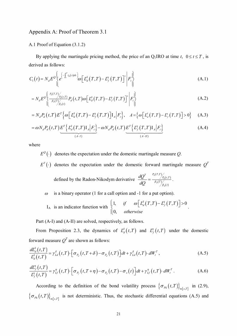
Q1IREO pricing is expressed in the following theorem, and the proof is provided in
Appendix A.
Theorem 3.1 The pricing formula of Q1IREOs with the final payoff as specified in (3.1.1 ) is
expressed as follows:
10
1 1, , , ,
1 11 12, , ,T T
d ft tu T T du u T T du
d d d fC t N P t T L t T e N d L t T e N d
(3.1.2)
where
2
1 1 1
111
, 1ln , , , ,, 2
Tdd ft
f
L t Tu T T u T T du V
L t Td
V
12 11 1d d V
2 21 , ,
T
Ld LftV u T u T du
1 , , , , ,d d
s sP PLdd t T T t T t T t T
1 , , , , ,f d
s sP PLf xf t T T t T t T t T t
1 (a call) or -1 (a put).
and , , ,sPk t k d f is defined as (A.7) in Appendix A.
The pricing equation (3.1.2) may be regarded as a generalized representation of Margrabe
(1978) in the framework of the cross-currency LMM. Note that when both compounding
periods are identical ( ), the pricing formula (3.1.2) reduces to the pricing model of a
regular option on the spread between the domestic and the foreign LIBOR rates in the
cross-currency LMM framework.
Theorem 3.1 not only provides the pricing formula for the Q1IREOs but also reveals a
clue to the construction of a hedging (replicating) portfolio for the Q1IREOs.
For hedging, we rewrite equation (3.1.2) as equation (3.1.3) (the proof is provided in
Appendix A) as follows
1 11 1 2, , , ,t d d t f fC t P t T P t T P t T P t T , (3.1.3)
where
1 , ,11 11
11 ,T
dtu T T du
t d dN L t T N d e
12 12 1
11 , ,t d dN L t T N d QA t T
1 1
,, ,
,d
f
P t TQA t T t T
P t T
1 , ,
1 ,T
ftu T T du
t T e
.
Equation (3.1.3) serves as a guide to the formation of a hedging portfolio 1tH for an
11
Q1IREO. 1tH can be completed by a linear combination of four types of assets: holding
long 11t units of ,dP t T and 1
2t units of ,fP t T and selling short 11t units of
,dP t T and 12t units of ,fP t T .
The term 1 ,QA t T appearing in (3.1.3) denotes the quanto adjustment due to the
hedged risk of the exchange rate. This exchange rate adjustment is induced by the fact that
expected foreign cash flow is derived under the domestic martingale measure, and by the
compound correlations between all the involved factors (the domestic and foreign bonds and
the exchange rate).
It is worth noting that the advantage of adopting the cross-currency BGM model rather
than other traditional models is that all the parameters as shown in (3.1.1) and (3.1.2) can be
easily obtained from market quotes, which makes the pricing formula more tractable and
feasible for practitioners.
3.2 Valuation of Second-Type QIREOs
Definition 3.2 A contingent claim with the payoff as specified in (3.2.1) is called a
Second-Type QIREO (Q2IREO)
2 , ,f f fC T X N L T T L T T , (3.2.1)
where
fN = notional principal of the option, in units of foreign currency
X = the fixed exchange rate expressed as the domestic currency value of one unit of foreign currency.
An Q2IREO is an option written on the difference between two foreign LIBOR rates with
different compounding periods and , but the final payment is measured in domestic
currency. From the viewpoint of domestic investors, holding an Q2IREO acts in much the
same way as longing a foreign yield-spread option, whose payoff is based on the difference
between the two underlying foreign interest rates, denominated in foreign currency, and
converting the foreign-currency payoff via multiplying the fixed exchange rate into the
domestic-currency payoff.
Using Q2IREOs has several benefits and applications. Domestic investors can benefit
from utilizing a corresponding Q2IREO with making a correct estimate of the differential
between two foreign LIBOR rates at some particular time point, thereby avoiding exposure to
12
exchange rate risk. For multinational enterprises or managers of cross-currency financial
assets, Q2IREOs can be used to enhance the interest profit of foreign assets or to reduce the
interest cost arising from foreign liabilities without incurring exchange rate risk. Furthermore,
Q2IREOs can be used to limit the downside risks of some particular payments if a manager of
cross-currency financial assets wants to manage the risk of foreign interest rate spread via a
long-period foreign basis swap involving the exchange of two series of floating-rate cash
flows in the same foreign currency.
The pricing formula of Q2IREOs is expressed in Theorem 3.2 below and the proof is
provided in Appendix B.
Theorem 3.2 The pricing formula of Q2IREOs with the final payoff as specified in (3.2.1) is
presented as follows:
2 2, , , ,
2 21 22, , ,T T
f ft tf d
u T T du u T T du
f fX N P t TC t L t T e N d L t T e N d
(3.2.2)
where
2
2 2 2
212
, 1ln , , , ,, 2
Tff ft
f
L t Tu T T u T T du V
L t Td
V
22 21 2d d V
2 22 , ,
T
Lf LftV u T u T du
2 , , , , , , ,f d
s sP PLf xf t T T t T t T t T t
.
Longstaff (1990), Fu (1996) and Miyazaki and Yoshida (1998) have derived the pricing
formulae for interest rate difference options, which are written on the underlying difference
between two domestic interest rates and denominated in domestic currency. In comparison
with their pricing formulae, the major differences between Theorem 3.2 and their formulae lie
in the fact that not only the “quanto-effect” is considered in Theorem 3.2, but also all
parameters appearing in Theorem 3.2 can be extracted from market quotes, which makes our
pricing formula more tractable and feasible for practitioners.
Once again, equation (3.2.2) can be written in terms of (3.2.3), and the proof is presented
in Appendix B.
2 22 1 2, , , ,t f f t f fC t P t T P t T P t T P t T , (3.2.3)
13
where
21 21 2
11 , ,t f dX N L t T N d QA t T
22 22 2
11 , ,t f dX N L t T N d QA t T
2 2
,, , , ,
,d
f
P t TQA t T t T
P t T
2 , ,
2 , , ,T
ftu T T du
t T e
.
Equation (3.2.3) shows the composition of a hedging portfolio 2tH for an Q2IREO: it
holds long 21t units of ,fP t T and 2
2t units of ,fP t T and sells short 21t units
of ,fP t T and 22t units of ,fP t T . The implication of the quanto adjustment
2 ,QA t is similar to 1 ,QA t T as mentioned above.
3.3 Valuation of Third-Type QIREOs
Definition 3.3 A contingent claim with the payoff as specified in (3.3.1) is called a
Third-Type QIREO (Q3IREO)
3 , ,f f fC T X T N L T T L T T , (3.3.1)
where
X T = the floating exchange rate expressed as the domestic currency value of one unit of foreign currency at time T.
An Q3IREO is analogous to the Q2IREO as specified in Subsection 3.2, but with the fixed
exchange rate X replaced by the floating exchange rate X T at maturity T. The structure
of an Q3IREO is slightly different from that of an Q2IREO in that this option is directly
affected by movements in the exchange rate. If the exchange rate moves upward, an investor
using this option could enhance profits from the difference between both the foreign interest
rates and the exchange rate. And a seller of this option could reduce payments due to
downward movements in a foreign currency’s value.
Since the Q3IREO can be priced in a similar way as the Q2IREO, we omit the proof. The
result is available upon request from the authors.
Theorem 3.3 The pricing formula of Q3IROs with the final payoff as expressed in (3.3.1 ) is
presented as follows:
14
3 3
3 31 32
, , , ,, , ,
T Tf ft t
f f f f
u T T du u T T duC t X t N P t T L t T N d L t T N de e
, (3.3.2)
where
2
3 3 3
313
, 1ln , , , ,, 2
Tff ft
f
L t Tu T T u T T du V
L t Td
V
32 31 3d d V
2 23 , ,
T
Lf LftV u T u T du
3 , , , , , , ,f f
s sP PLff t T T t T t T t T
.
Similarly, we rewrite (3.3.2) to obtain (3.3.3) as follows
3 33 1 2, , , ,t f f t f fC t P t T P t T P t T P t T , (3.3.3)
where
3 , ,31 31
11 ,T
ftu T T du
t f fX t N L t T e N d
3 , ,32 32
11 ,T
ftu T T du
t f fX t N L t T e N d
.
Equation (3.3.3) also implies a composition for a hedging portfolio 3tH similar to that
given in the previous theorems. It is worth noting that the quanto adjustment disappears in
(3.3.3), since the exchange rate risk in the Q3IREO is unhedged; this option is directly
affected by unanticipated changes in the exchange rate.
3.4 Valuation of Fourth-Type QIREOs
Definition 3.4 A contingent claim with the payoff as specified in (3.4.1) is called a
Fourth-Type QIREO (Q4IREO)
4 , ,f f d dC T X T N L T T N L T T
. (3.4.1)
= a binary operator (1 for a call option and -1 for a put option).
An Q4IREO is an option written on the difference between a foreign interest payment
based on the foreign LIBOR rate with a compounding period and a domestic interest
payment based on the domestic LIBOR rate with a compounding period .
This option is slightly different from those options described in the above subsections. It
can be considered as an option to exchange domestic-currency-denominated interest
15
payments for foreign-currency-denominated interest payments.
Theorem 3.4 below presents the pricing formula of an Q4IREO. Its proof follows in a
similar way as the previous options. The result is available upon request from the authors.
Theorem 3.4 The pricing formula of Q4IREOs with the final payoff as expressed in (3.4.1 ) is
presented as follows:
4
4
, ,
4 41
, ,
42
, ,
, ,
Tgt
Tdt
u T T du
f f f
u T T du
d d d
C t X t N P t T L t T e N d
N P t T L t T e N d
(3.4.2)
where
2
4 4 4
414
, , 1ln , , , ,, , 2
Tf f fg dt
d d d
X t N P t T L t Tu T T u T T du V
N P t T L t Td
V
42 41 4d d V
2 24 , ,
T
g LdtV u T u T du
4 , , , , ,f f
s sP PLfg t T T t T t T t T
4 , , , , ,d d
s sP PLdd t T T t T t T t T
.
In order to obtain a hedging portfolio, equation (3.4.2) is rewritten as equation (3.4.3).
4 44 1 2, , , ,t f f t d dC t P t T P t T P t T P t T , (3.4.3)
where
4 , ,41 41
11 ,T
gtu T T du
t f fX t N L t T e N d
4 , ,42 42
11 ,T
dtu T T du
t d dN L t T e N d
.
Equation (3.4.3) shows the composition of a hedging portfolio 4tH for an Q4IREO:
holding long 41t units of ,fP t T and 4
2t units of ,dP t T and selling short 41t
units of ,fP t T and 42t units of ,dP t T . Due to the unhedged exchange-rate risk
inherent in the Q4IREO, the quanto adjustment does not exist in equation (3.4.3) as in the
case examined in Subsection 3.3; this option is directly affected by exchange-rate movements
as well.
16
In Section 4, we provide a calibration procedure and numerical examples showing the
accuracy of the pricing formulae.
4. Calibration Procedure and Numerical Examples
In this section, we first provide a calibration procedure and then examine the accuracy of
the pricing formula via a comparison with Monte Carlo simulation.
4.1 Calibration Procedure
With the advantage of the pricing formulae for caps and floors which are consistent with
the popular Black formula [1976], the cross-currency LIBOR market model is easier for
calibration. We employ the mechanism presented by Rebonato [1999] to engage in a
simultaneous calibration of the cross-currency LIBOR market model to the percentage
volatilities and the correlation matrix of the underlying forward LIBOR rates and the
exchange rate.
Assume that there are n domestic forward LIBOR rates, n foreign forward LIBOR rates
and an exchange rate in an m-factor framework. The steps to calibrate the model parameters
are presented as follows:
First, as given in Brigo and Mercurio [2001], we assume that the domestic forward
LIBOR rate, ,dL t , has a piecewise-constant instantaneous total volatility structure
depending only on the time-to-maturity (i.e., ,d d
i j i jV ). The elements in Exhibit 1, which
specify the instantaneous total volatility applied to each period for each rate, can be stripped
from market data. A detailed computational process is presented in Hull [2003].
The case of the foreign forward LIBOR rate, ,fL t , can be carried out in a way similar
to the domestic case. In addition, we also assume that the exchange rate X t has a
piecewise-constant instantaneous total volatility structure. The elements in Exhibit 2, which
represent the instantaneous total volatility applied to each period for the exchange rate, can be
calculated from the prices of the on-the-run options in the market. However, the durations of
the exchange rate options are usually shorter than one year, so the market-obtainable
elements in Exhibit 2 are usually not sufficient for pricing interest options. This problem may
17
be resolved by using the implied (or historical) volatility of the underlying exchange rate, and
assuming that the term structure of volatilities is flat (i.e., X Xt for 0( , ]nt t t ).
Exhibit 1: Instantaneous Volatilities of ,,k k d f
L t
Instant. Total Vol. Time 0 1( , ]t t t 1 2( , ]t t 2 3( , ]t t … 2 1( , ]n nt t
Fwd. Rate: 1,kL t t 1,1 0k kV Dead Dead … Dead
2,kL t t 2,1 1k kV 2,2 0
k kV Dead … Dead
… … … … … …
1,k nL t t 1,1 2k k
n nV 1,2 3k k
n nV 1,3 4k k
n nV … 1, 1 0k k
n nV
Exhibit 2 : Instantaneous Volatilities of the Exchange Rate
Instant. Total Vol. Time 0 1( , ]t t t 1 2( , ]t t 2 3( , ]t t … 2 1( , ]n nt t
Fwd. Rate: X t 1 1XV 2 2XV 3 3XV … Xn nV
Second, we use the historical price data of the domestic and foreign forward LIBOR rates
and the exchange rate to derive a full-rank (2n+1)×(2n+1) instantaneous-correlation matrix
. Thus, is a positive-definite symmetric matrix and can be written as
'H H
where H is a real orthogonal matrix and is a diagonal matrix. Let 1/ 2A H and thus
'AA . In this way, we can find a suitable m-rank matrix B such that the m-rank matrix
'B BB can be used to mimic the market correlation matrix , where m ≤ 2n+1.
The purpose of the second step is to replace the 2n+1-dimensional original Brownian
motions dW t with BdZ t , where dZ t is a vector of m-dimensional Brownian
motions. In other words, we change the market correlation structure
'dW t dW t dt
to a modeled correlation structure
' ' ' ' BBdZ t BdZ t BdZ t dZ t B BB dt dt
The remaining problem is how to choose a suitable matrix B. Rebonato [1999] proposed
the following form for the ith row of B :
18
1
, 1 ,, 1
1 ,
cos sin 1,2,..., 1
sin
ki k j i j
i k kj i j
if k mb
if k m
for 1,2,...,2 1i n . By finding a that solves the optimization problem
2
, ,, 1
minn
Bi j i j
i j
and substituting into B , we obtain a suitable matrix B such that 'B BB is an
approximate correlation matrix for .
Third, B can be used to distribute the instantaneous total volatility to each Brownian
motion at each period for the exchange rate and to each LIBOR rate without changing the
amount of the instantaneous total volatility. That is,
, 1 2,1 , , 2 ,..., , , , , ,..., , ,ki j Lk i Lk i Lkm iV B i B i B i m t t t t t t
1 2,1 , ,2 ,..., , , ,..., ,j X X XmB n B n B n m t t t
where 1, 2,..., 1i n and 1( , ]j jt t t , for each 1, 2,...,j n .
Under the assumption that the instantaneous total volatility structures are
piecewise-constant, the previous procedure represents a general calibration method without a
constraint on choosing the number of factors. Via the distributing matrix B , the individual
instantaneous volatility applied to each Brownian motion at each period for each process can
be derived. With these data calibrated from the market correlation matrix and volatilities, we
can employ Monte Carlo simulation to price any associated interest rate derivatives. The data
can also be used to calculate the prices of the QIREOs as derived in Theorems 1, 2, 3 and 4.
4.2 Numerical Analysis
This subsection offers some practical examples that examine the accuracy of the pricing
formulas as derived in the previous section and compare the results with Monte Carlo
simulation. Based on actual market data, as shown in Exhibits 5 to 10 in Appendix C, the
1-year and 3-year Q2IREOs with 12 year and 1 in Theorem 1 are priced at
different semiannually dates, and the results are listed in Exhibits 3 and 4. The flat volatility
of the exchange rate is assumed to be 20%. The notional value is assumed to be $1. The
19
simulation is based on 50,000 sample paths. Note that in the examples, the domestic country
is the U.S. and the foreign country is the U.K. By comparison to Monte Carlo simulation, the
pricing formulas have shown to be accurate and robust for the recent market data. The
empirical examples associated with the other three theorems have also shown satisfactory
s.e. 1.2812×10⁻⁵ 1.2560×10⁻⁵ 2.3516×10⁻⁵ 2.8212×10⁻⁵ The prices of a 1-year Q1IRO with semiannual accrual periods are presented in this exhibit. The abbreviations
M.C. and s.e. represent the results of Monte Carlo simulations and their standard errors, respectively.