31
Quantum Algorithms for Applied Mathematics Stephen Jordan Feb 17, 2015

Quantum Algorithms forApplied Mathematics
Stephen Jordan
Feb 17, 2015

Quantum Algorithms
● Linear Algebra● Integrals & Sums● Optimization● Simulation of Physical Systems● Graph theory● Number Theory● Search and Boolean Formula Evaluation● Topological Invariants
math.nist.gov/quantum/zoo/

Quantum Algorithms
● Linear Algebra● Integrals & Sums● Optimization● Simulation of Physical Systems● Graph theory● Number Theory● Search and Boolean Formula Evaluation● Topological Invariants
math.nist.gov/quantum/zoo/
This talk
Alán's talk
Linear Algebra
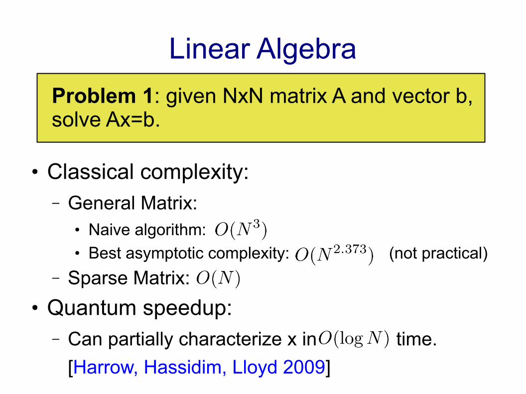
● Classical complexity:– General Matrix:
● Naive algorithm:● Best asymptotic complexity: (not practical)
– Sparse Matrix:● Quantum speedup:
– Can partially characterize x in time.
[Harrow, Hassidim, Lloyd 2009]
Problem 1: given NxN matrix A and vector b,solve Ax=b.
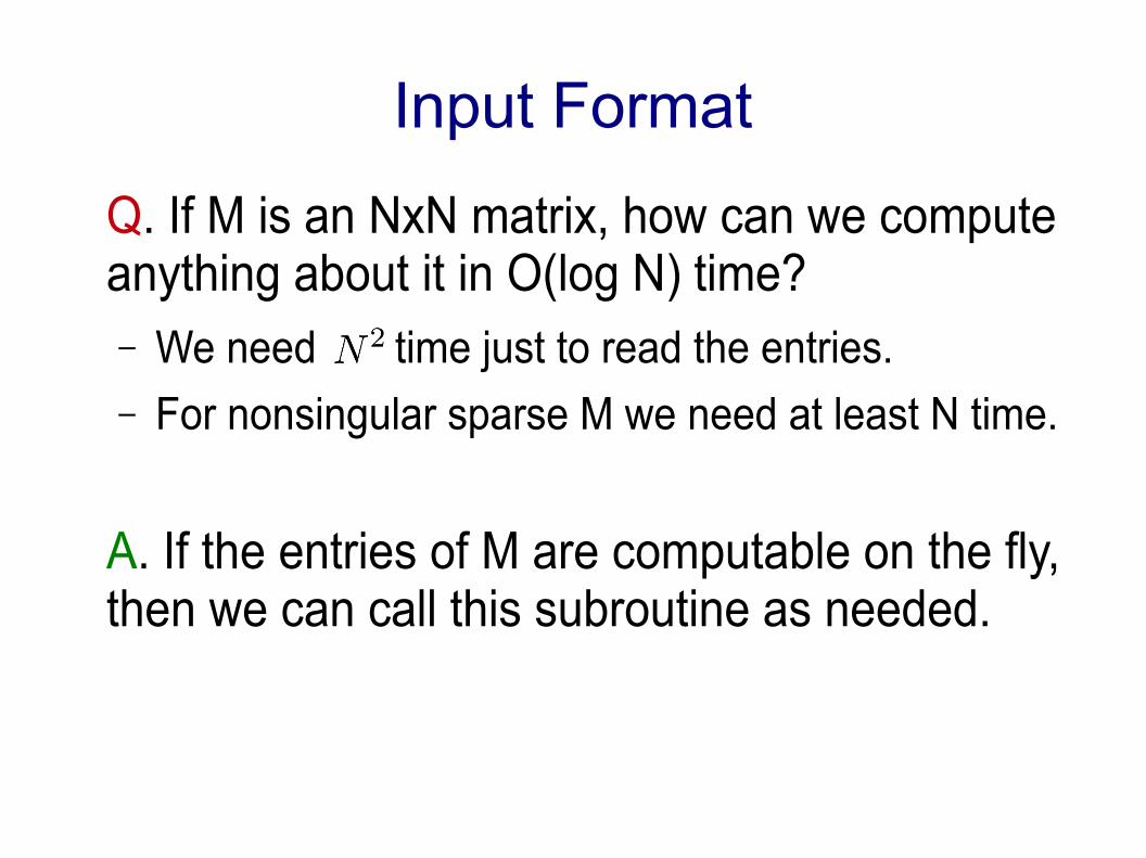
Input Format
Q. If M is an NxN matrix, how can we compute anything about it in O(log N) time?– We need time just to read the entries.– For nonsingular sparse M we need at least N time.
A. If the entries of M are computable on the fly, then we can call this subroutine as needed.

HHL Quantum Algorithm
● Physics:
● Quantum algorithms for simulation [Alán's talk]– For physical on n qubits, can usually
be implemented with poly(n,t) quantum gates.– Matrix computation by quantum computation...
Hamiltonians arising in nature are structured and sparse.

HHL Quantum Algorithm
Harrow Hasidim & Lloyd showed this primitive:
can be used to construct a state:
Problem 1: given NxN matrix A and vector b,solve Ax=b.
make
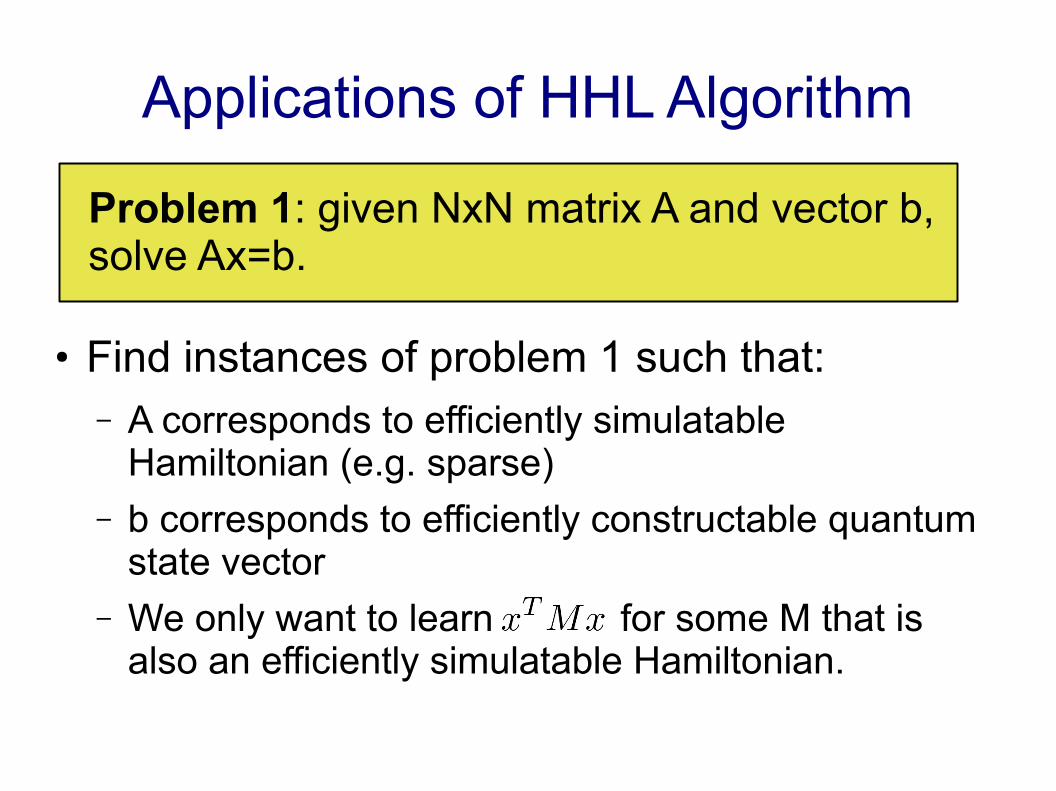
Applications of HHL Algorithm
● Find instances of problem 1 such that:– A corresponds to efficiently simulatable
Hamiltonian (e.g. sparse)– b corresponds to efficiently constructable quantum
state vector– We only want to learn for some M that is
also an efficiently simulatable Hamiltonian.
Problem 1: given NxN matrix A and vector b,solve Ax=b.

Applications of HHL Algorithm
Several applications have been proposed for the HHL algorithm and its variants*:
● Solving linear differential equations [Berry, 2010]
● Least-squares curvefitting[Wiebe, Braun, Lloyd, 2012]
● Machine learning[Lloyd, Mohseni, Rebentrost, 2013][Lloyd, Garnerone, Zanardi, 2014]
● Matrix inversion in logarithmic space[Ta-Shma, 2013]
*dependence on condition number of M has been improved from to in [Ambainis, 2010]
Can you find more?

Integrals & Sums
● Classical randomized sampling:
● Quantum amplitude amplification:[Brassard, Hoyer, Tapp, 1998] [Mosca, 1998]
– This is optimal. [Nayak, Wu, 1999]
– Generalizes to integrals. [Novach, 2000]
Problem 2: given black-box access to
approximate within .
Optimization
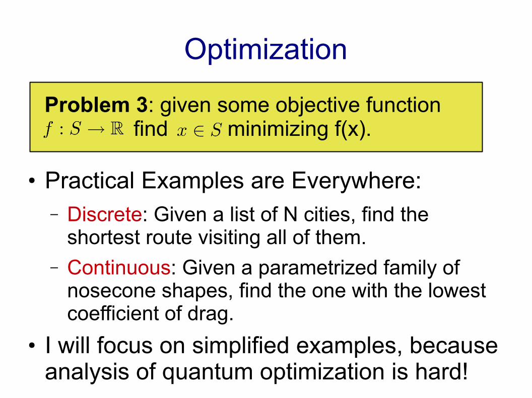
Problem 3: given some objective function find minimizing f(x).
● Practical Examples are Everywhere:– Discrete: Given a list of N cities, find the
shortest route visiting all of them.– Continuous: Given a parametrized family of
nosecone shapes, find the one with the lowest coefficient of drag.
● I will focus on simplified examples, because analysis of quantum optimization is hard!

Optimization
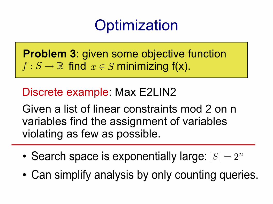
Problem 3: given some objective function find minimizing f(x).
Discrete example: Max E2LIN2
Given a list of linear constraints mod 2 on n variables find the assigment of variables violating as few as possible.
1
0
1

Optimization
Problem 3: given some objective function find minimizing f(x).
Discrete example: Max E2LIN2
Given a list of linear constraints mod 2 on n variables find the assigment of variables violating as few as possible.
1
0
1
Optimal: violate 1.
Optimization
Problem 3: given some objective function find minimizing f(x).
Discrete example: Max E2LIN2
Given a list of linear constraints mod 2 on n variables find the assignment of variables violating as few as possible.
● Search space is exponentially large:● Can simplify analysis by only counting queries.

Complexity of Optimization
Theorem: If f is completely unstructured
(e.g. random ranking )
then the optimal strategy is:
Classical: Brute search
Quantum: Grover's algorithm
[Nayak, Wu, 1998]

Complexity of Optimization
In practice, the search space usually has some topology relative to which the objective function is smooth or structured.
Example:
Easy Challenging Unstructured

Complexity of Optimization
In practice, the search space usually has some topology relative to which the objective function is smooth or structured.
Example:
Easy Challenging Unstructured
Complexity of Optimization
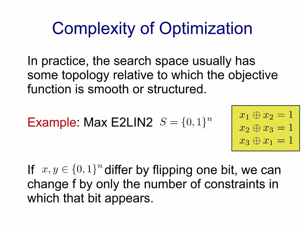
In practice, the search space usually has some topology relative to which the objective function is smooth or structured.
Example: Max E2LIN2
If differ by flipping one bit, we can change f by only the number of constraints in which that bit appears.
Gradient Descent
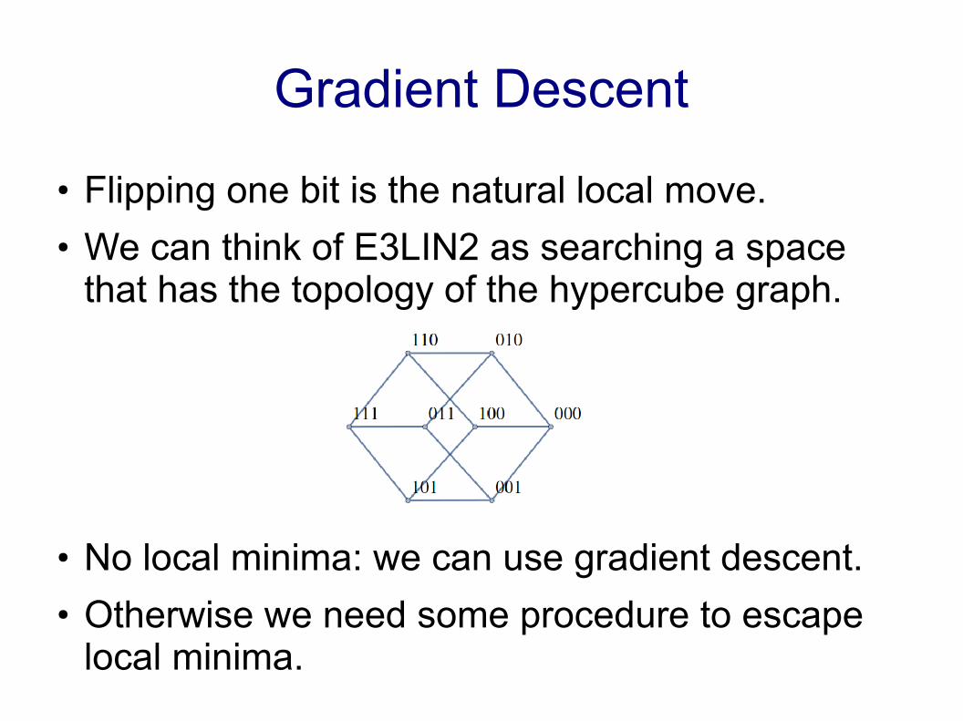
● Flipping one bit is the natural local move.● We can think of E3LIN2 as searching a space
that has the topology of the hypercube graph.
● No local minima: we can use gradient descent.● Otherwise we need some procedure to escape
local minima.
Simulated Annealing
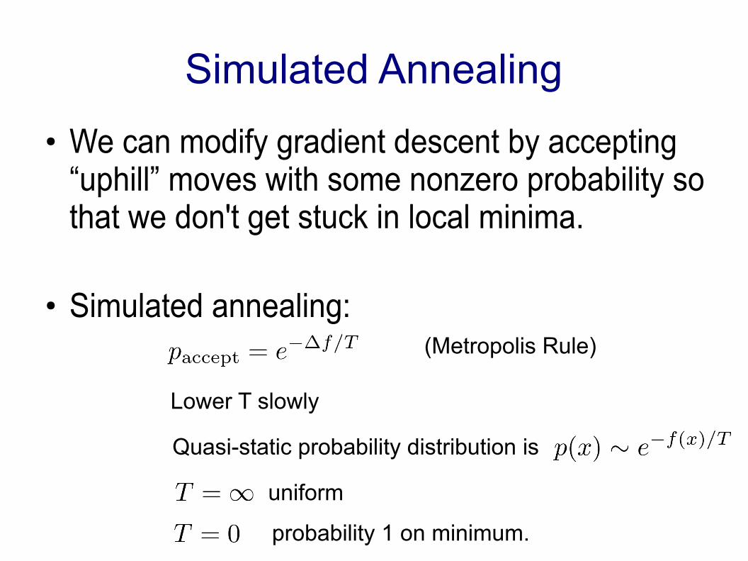
● We can modify gradient descent by accepting “uphill” moves with some nonzero probability so that we don't get stuck in local minima.
● Simulated annealing:
Lower T slowly
(Metropolis Rule)
Quasi-static probability distribution is
uniform
probability 1 on minimum.
Adiabatic Quantum Computation
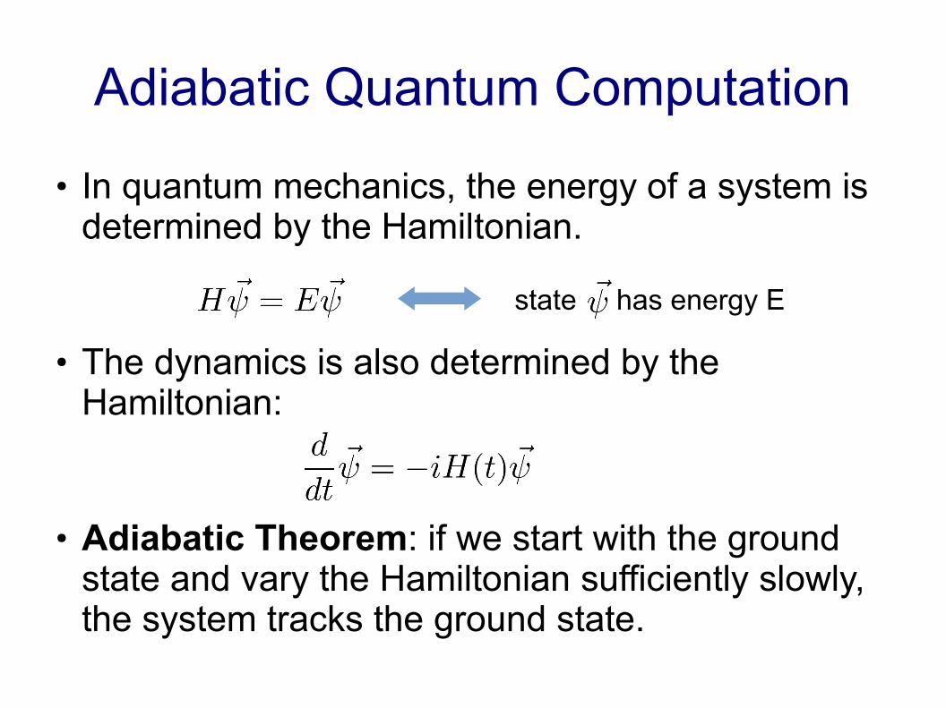
● In quantum mechanics, the energy of a system is determined by the Hamiltonian.
● The dynamics is also determined by the Hamiltonian:
● Adiabatic Theorem: if we start with the ground state and vary the Hamiltonian sufficiently slowly, the system tracks the ground state.
state has energy E
Adiabatic Quantum Computation
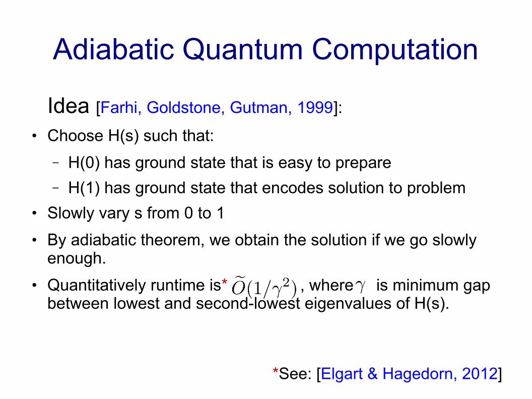
Idea [Farhi, Goldstone, Gutman, 1999]:
● Choose H(s) such that:
– H(0) has ground state that is easy to prepare
– H(1) has ground state that encodes solution to problem● Slowly vary s from 0 to 1
● By adiabatic theorem, we obtain the solution if we go slowly enough.
● Quantitatively runtime is* , where is minimum gap between lowest and second-lowest eigenvalues of H(s).
*See: [Elgart & Hagedorn, 2012]
Adiabatic Optimization
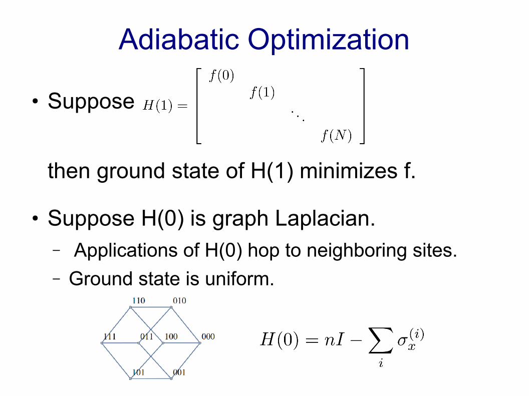
● Suppose
then ground state of H(1) minimizes f.
● Suppose H(0) is graph Laplacian.– Applications of H(0) hop to neighboring sites.– Ground state is uniform.

Adiabatic vs. Thermal
Thermal Adiabatic
Probability distribution Quantum Superposition
Quasi-static:stay in Gibbs distribution
Quasi-static:Stay in ground state
Decrease Temperature Decrease Hopping Term

Adiabatic vs. Thermal
● Consider a one-dimensional double well:
● Thermal annealing: Boltzman factor● Adiabatic optimization: tunneling matrix element● These are different, so adiabatic can outperform
thermal annealing.● Better examples (on hypercube):
[Farhi, Goldstone, Gutmann, 2002] [Reichardt, 2004]

Adiabatic Optimization
● Evaluating the eigenvalue gap is hard.– Numerics break down at n ~ 20-100– Analytic techniques mainly for high symmetry– Gap can be exponentially small even for easy problems
with no local minima [Jarret, Jordan, 2014]
● What to do?– More math [cf. Altschuler, Krovi, Roland, 2007]
– Try more general setting: go faster adiabatic theorem recommends and/or allow interaction with environment[cf. Nagaj, Somma, Kieferova, 2012]
– Try experiments [cf. Boixo et al, 2013]

Hogg's Algorithm
● Classical: n queries
● Quantum: 1 query
[Hogg, 1998]
Problem 4: Given black box forwith promise , find using asfew queries as possible.
Gradients and Quadratic Basins
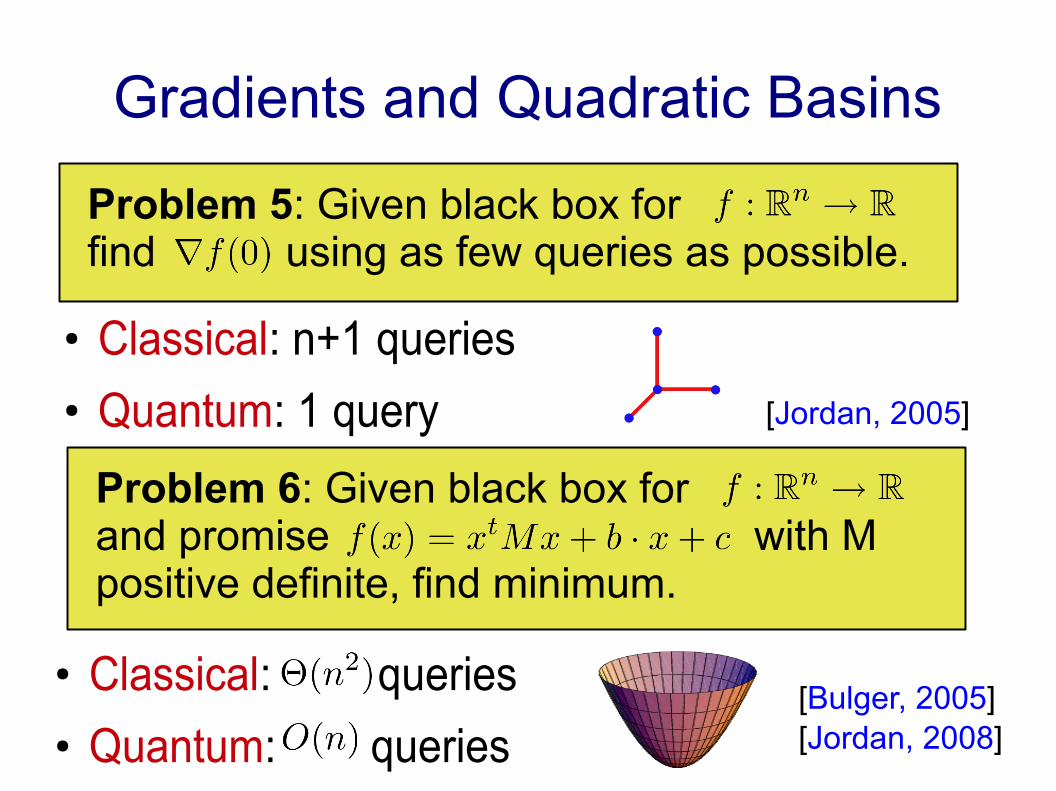
Problem 5: Given black box forfind using as few queries as possible.
● Classical: n+1 queries● Quantum: 1 query
Problem 6: Given black box forand promise with Mpositive definite, find minimum.
● Classical: queries● Quantum: queries
[Jordan, 2005]
[Bulger, 2005][Jordan, 2008]

Very Recent Breakthrough
Problem 6 (“E3LIN2”): Given a list of N linearequations mod 2, satisfy as many as possible.Each equation involves exactly 3 variables.Each variable is in at most D equations.
● Classical: satisfy
● Quantum: satisfy
● NP-hard: satisfy
[Farhi, Goldstone, Gutmann, 2014]

Summary● Linear Algebra:
– Can solve N linear equations in log N time– Needs special structure (e.g. sparsity)
● Sums and Integrals:– Can obtain precision in time.– Quadratic speedup by generalizing Grover's algorithm.
● Optimization:– Adiabatic optimization: promising but mysterious.– Factor of d speedups for symmetric d-dimensional
optimization problems.– Recent breakthrough achieves better approximation factor
for E3LIN2 than any classical polynomial-time algorithm.


