Quantum circuit optimization by topological compaction in the

surface code

Adam PaetznickDavid R. Cheriton School of Computer Science, and

Institute for Quantum Computing,University of Waterloo

Austin G. FowlerCentre for Quantum Computation and Communication Technology,

School of Physics,The University of Melbourne

Abstract

The fragile nature of quantum information limits our ability to construct large quantities ofquantum bits suitable for quantum computing. An important goal, therefore, is to minimizethe amount of resources required to implement quantum algorithms, many of which are serial innature and leave large numbers of qubits idle much of the time unless compression techniquesare used. Furthermore, quantum error-correcting codes, which are required to reduce the effectsof noise, introduce additional resource overhead.

We consider a strategy for quantum circuit optimization based on topological deformation inthe surface code, one of the best performing and most practical quantum error-correcting codes.Specifically, we examine the problem of minimizing computation time on a two-dimensionalqubit lattice of arbitrary, but fixed dimension, and propose two algorithms for doing so.

1 Introduction

The task of building a large-scale quantum computer is a challenging one. Quantum informationtends to decohere quickly, and thus our ability to construct and manipulate quantum bits (qubits)in large quantities is limited. An important goal, therefore, is to minimize the number of qubitsand the amount of time required to implement quantum algorithms. However, many quantum algo-rithms are serial in nature, leaving large numbers of qubits idle much of the time. Low-gate-countarithmetic quantum circuits, for example, form a staircase structure of linear depth [CDKM04].Parallelization of certain procedures, such as the quantum Fourier transform, is possible when extraqubits are available but is typically done on a case by case basis [CW00].

Error-correcting codes are required in order to reduce the impact of decoherence and faultycontrol of the computer [Sho96]. While it is possible introduce error-correction without inducingtime overhead [Fow12b], any fault-tolerant circuit will require an increase in either time or space ascompared to the corresponding ideal quantum circuit. The resource increase can be very large, oftenas much as a million fold or more [Kni05, RHG07, PR12, JVF+12]. Resource estimates are evenlarger if geometric constraints of the quantum computer are considered. Indeed, many proposals for

1

arX

iv:1

304.

2807

v1 [

quan

t-ph

] 9

Apr

201

3

quantum computers impose a fixed-size two-dimensional lattice, with limited interactions betweenqubits [Lev01, WHL05, DFS+09, HMF+09, DiV09, AUW+10, JVF+12, KBB11, LCG+11, KL13].

We propose an automated and global resource optimization solution which is fault-tolerant andaccounts for geometry and locality constraints by operating within the surface code. Our strategy isto minimize computation time by smoothly reshaping the computation in order to eliminate wastedspace. Two algorithms are presented. The first is a force-directed algorithm in which the fault-tolerant quantum circuit is treated as a malleable physical object. The second algorithm is basedon simulated annealing. Each algorithm takes as input an ideal quantum circuit and a fixed-sizetwo-dimensional qubit lattice and outputs a corresponding compact fault-tolerant quantum circuitthat operates entirely within the lattice dimensions.

A variety of techniques have been proposed for reducing resource overhead in fault-tolerantquantum circuits. For schemes based on concatenated codes, the overhead is dominated by er-ror correction circuits which require carefully prepared encoded states. Efficient techniques forpreparing such states have been developed and continue to improve [Ste04, Rei06, PR12]. Anothersignificant source of overhead is the execution of particular gates that are required for universality.These gates involve preparation and distillation of exotic resource states [BK04]. Recently therehave been a number of proposals for improving the efficiency of distillation [MEK13, BH12, Jon12,FD12, FDJ13].

The above techniques have been effective at reducing the resources required by fault-tolerantquantum circuits. However, they are largely manual, and focus on a small but repeated part of thecircuit. They do not address, for example, global parallelism concerns.

Some techniques for pararallelization exist. Typical methods involve local circuit rewriting rulesfor trading between sequences of gates and additional qubits [MN01, MDMN08, SWD10]. Small-depth circuits can be achieved for certain sub-classes of quantum circuits. Clifford group circuits, forexample, can be parallelized to quantum circuits of constant depth followed by log-depth classicalpost-processing [RB01].

Others have proposed global circuit optimization procedures that involve a multi-staged trans-formation to and from the measurement-based quantum computing model [BK09, dSPK13]. Indeed,there are strong similarities between the measurement-based model and the surface code [RH07].However, the template-based and measurement-based optimizations are not fault-tolerant and,except for [SWD10], do not explicitly consider geometric constraints imposed by the quantumcomputer. It is not clear that the resulting circuits remain compact under such restrictions.

Alternatively, since our algorithms operate within the surface code, the output is automaticallyfault-tolerant and can be easily mapped to a wide variety of two-dimensional nearest-neighborarchitectures [DiV09, GFG12]. Furthermore, the rules for topologically transforming surface codebraids are conceptually simple. There is no need to break up the transformation into multiplestages. Thus, compared to other proposals, we feel that our approach is easier to understand,implement, and extend.

That is not to say that braid compaction is computationally easy, however. In fact, basedon known complexities of other similar problems such as VLSI placement [SLW83] and containerloading (see, e.g., [Sch92]), we conjecture that the problem of minimizing the time (height) of abraid on a fixed rectangular lattice of qubits is NP-complete. Our optimization algorithms aretherefore crafted from carefully designed heuristics in order to handle large-scale instances.

The first algorithm is loosely based on the physical principles of gravity and tension. Roughly,the braid is treated as a heavy tangle of rubber bands that is allowed to slide into a box under

2

the force of gravity. The idea is vaguely analogous to techniques used in graph drawing, forexample [Kob12]. The second algorithm uses the technique of simulated annealing. In simulatedannealing the solution landscape is explored by making random incremental changes and favoringthose changes which decrease the solution size. Our algorithm is inspired by a similar procedurefor VLSI placement [HLL88].

We begin with a brief summary of the surface code in Section 2 followed by a more formalstatement of the braid compaction problem in Section 3. In Section 4 we describe the force-directed algorithm in detail, and a C++ implementation that we call Braidpack. The simulatedannealing algorithm is presented in Section 5.

2 The surface code

In this section, we give a brief pedagogical introduction to the surface code. The focus here is onthe mapping from a quantum circuit to a surface code braid. Other details of the surface code arenot essential for understanding our braid compaction algorithms. For a comprehensive introductionto the surface code we refer the reader to [FMMC12].

The surface code has a number of desirable properties. First, it operates on a two-dimensionalrectangular lattice of qubits. All operations can be performed using only one-qubit gates, andtwo-qubit gates involving only nearest neighbor qubits. As a result, the required number of qubitsscales much more slowly for the surface code than for concatenated codes on 2-D nearest-neighborarchitectures. At the same time, the surface code tolerates noisier physical gates than many otherquantum error correcting codes. Reliable computation is possible so long as the noise rate is belowroughly 0.6 percent per gate.

Error-correction is performed by periodically measuring four-qubit operators, known as stabiliz-ers, around each face and and each vertex of the lattice. Codewords correspond to the simultaneous±1-eigenstates of the operators. Each measurement imposes a restriction on the Hilbert space ofthe lattice. Encoded qubits are created by disabling some of the measurements, thereby addingnew degrees of freedom. We choose to define a qubit as a pair of defects. Defects are contiguousregions of the lattice for which the stabilizers are not measured. There are two types of defects,primal and dual. Primal defects correspond to operators around vertices of the lattice, and dualdefects correspond to operators around the faces of the lattice.

Error protection is achieved by creating defects of sufficient size, and by keeping defects wellseparated in space. For a code distance of d, we require that all defects have circumference d andthat defects of the same type are separated in L∞ distance by d. For defects of opposite type, theminimum distance depends on the shape of each defect. In all cases a distance of d/4 is sufficient,though in some cases primal and dual defects may be as close as d/8.

Most encoded operations in the surface code proceed by moving defects around each other.Defect movement is achieved by turning off new regions of stabilizer measurements and then turningon other stabilizer measurements. The movement can be divided into time-slices. By stackingtime-slices on top of each other, the encoded operations are represented by a three-dimensionalobject in space and time called a braid. See Figure 1. Transformation of a quantum circuit toa braid can be done systematically by constructing canonical braid elements for each quantumgate. Preparation of encoded |0〉 is represented by a “U”-shaped primal defect. Encoded Z-basismeasurement is essentially the reverse. A controlled-NOT (CNOT) operation is performed by aloop of dual defects that wraps around the two associated encoded qubits. See Table 1.

3

(a) top view

space

time

(b) side view

Figure 1: (a) Encoded surface code qubits are defined by pairs of defects, either primal (red) ordual (blue). Each defect is composed of multiple physical qubits on the two-dimensional lattice.Operations are performed by moving defects around. Here, an encoded two-qubit operation isperformed by moving one defect from the dual encoded qubit around one of the defects of theprimal encoded qubit. (b) The same operation can be written as a space-time diagram in whichone of the space axes has been flattened.

|0〉 Z

•H T

T

YYA

Table 1: The surface code gate set (top) and corresponding canonical braids (bottom). Each braidis a three-dimensional collection of defects. For visual clarity, the braids have been flattened hereinto two dimensions.

4

space

time

(a) (b)

Figure 2: Surface code braids are invariant under topological deformation. The space-time diagramon the left (a) is topologically equivalent to the diagram on the right (b). Defect strings and loopsmay be smoothly stretched and contracted without altering the encoded operation.

Braids consisting of these operations are invariant under topological deformation. That is, aquantum circuit can be represented by a canonical braid, and also by any braid that is topologicallyequivalent to that canonical braid. Strings of defects may be smoothly pulled or pushed around inspace and time without altering the encoded quantum computation. See Figure 2. Note that spaceand time are symmetric here. Space can be traded for time and vice versa.

Not all encoded operations in the surface code can be performed topologically, however. Theencoded Hadamard operation, for example, requires the encoded qubit—i.e., the two correspondingdefects—to be placed on a separate lattice, isolated from all other encoded qubits. This is achievedby first “cutting out” part of the lattice around the encoded qubit and then later re-attaching itto the rest of the lattice [Fow12a]. The resulting space-time volume is a cuboid (i.e., a box) ofdimension roughly 3d/2× 3d/2× 5d/2. However, the cuboid contains a variety of boundary typesnear the surface, thus imposing some restrictions on the configurations of other surrounding defects.The cuboid can be translated in any direction, or rotated about the time-axis by increments of π/2,but is otherwise treated as a rigid object.1 For concreteness, we adopt the convention that timecorresponds to the z-axis.

There is one other non-topological operation, the encoded T -gate which performs the rotation(1 00 eiπ/4

). This gate cannot be implemented directly in the surface code and is instead constructed

by a process known as state injection and distillation followed by gate teleportation [BK04]. Itdoes not explicitly require the encoded qubit to be cut out of the lattice, as the Hadamard does.However, both the distillation and gate teleportation involve measurements which are probabilistic.The required circuit changes depending on the measurement outcomes. See Figure 3a.

Likewise, the corresponding braid cannot be entirely determined ahead of time. It is possible,however, to shift all of the non-determinism either offline or into logical measurements, which can beperformed very efficiently [Fow12b]. Figure 3b shows an alternative circuit that also implements T .In this circuit, an S = ( 1 0

0 i ) gate, implemented with the help of a resource state |Y 〉 = 1√2(|0〉+i |1〉),

is selectively teleported into the circuit conditioned on the outcome of an Z-basis measurement.Given states |A〉 and |Y 〉, the entire circuit is determined ahead of time except for the measurementbases for selective teleportation.

The circuit in Figure 3a is smaller than that of Figure 3b. The latter circuit, however, has theadvantage that it can be composed in parallel with any number of additional T gate circuits. Thebraid corresponding to the single-qubit unitary THT , for example, can be parallelized as shown

1In principle, a sideways Hadamard gate is possible and would allow for rotations about the x and y axes. However,the chosen implementation requires the cuboid to be vertically oriented.

5

|A〉 • S T |ψ〉

|ψ〉 Z •(a)

|ψ〉 Z •

|A〉 • • Z/X

|0〉 X/Z

|Y 〉 H H |Y 〉

|+〉 • • • • X/Z

|+〉 • • Z/X

|0〉 T |ψ〉

(b)

Figure 3: Two circuits that implement the T gate on input state |ψ〉. (a) The resource state|A〉 = |0〉 + eiπ/4 |1〉 is constructed by injection and distillation. Conditioned on the measurementoutcome, a corrective S = ( 1 0

0 i ) rotation may be required, which requires a non-destructive useof an ancilla |Y 〉 = |0〉 + i |1〉 state, initially prepared by injection and distillation (not shown).(b) Instead of performing the conditional S gate directly, selective destination teleportation can beused [Fow12b]. On one path of the teleportation, the S gate is applied, and on the other path itis not. The Z-basis measurement on |ψ〉 determines the bases in which the other four qubits aremeasured. The output is T |ψ〉, up to Pauli corrections from teleportation.

in Figure 4. The logical measurements in this braid are implemented differently than previouslydiscussed. The cap on the defects has been flattened into a wider, but thinner set of defects thatlooks like a tabletop. This allows for maximum parallelization of sequences of T gates.

The measurement regions of Figure 4 must obey a relative time ordering. In particular, theZ-basis measurement of the input qubit |ψ〉 must be completed before the selective teleportationmeasurements can be performed. In addition, the selective teleportation of the previous T (ifapplicable) must be completed before selective teleportation measurements of current T gate canbe performed. In this way, the measurement regions for sequences of T gates form a tree. Eachmeasurement region must be located strictly later in time than each of its children.

There are a variety of options for preparing the |A〉 and |Y 〉 states required by Figure 3b. The|A〉 state, for example, can be prepared by a 15:1 injection and distillation procedure due to Bravyiand Kitaev [BK04], or one of several recent proposals [MEK13, BH12, Jon12]. Efficient surfacecode braids are known for several of these protocols [FD12, FDJ13], though we will not discussthe details here. Rather, for simplicity we abstract the |A〉 and |Y 〉 preparation as rigid cuboids,similar to the Hadamard gate. This gives us the freedom to define braid compaction algorithmswithout being coupled to a particular distillation procedure.

The gates listed in Table 1 are universal for quantum computing. Thus any quantum circuit canbe mapped to a surface code braid by first decomposing it into this gate set, and then sequentiallyconstructing each of the canonical braid elements.

3 The braid compaction problem

The canonical braid is a fault-tolerant representation of the original circuit, but there is no guaranteethat it will fit onto the two-dimensional lattice of qubits that is available. Indeed, the structureof the canonical braid closely resembles that of the original circuit. It is essentially a long line of

6

T H T(a)

T H T

A YY A YY(b)

Figure 4: (a) A quantum circuit for the single-qubit unitary THT in which time runs left to right.(b) A schematic representation of the corresponding surface code braid in which time runs bottomto top. For simplicity, the braids corresponding to Figure 3b are shown as boxes, except for themeasurements which are shown as thin tabletop structures. The T and H boxes may be placedin parallel, and the |A〉 and |Y 〉 states may be prepared ahead of time. The first measurement ofthe T gate must complete before the remaining four selective teleportation measurements can beperformed. Selective teleportation measurments between T gates also obey a relative time-orderingas indicated by the black dotted lines. Any sequence of single-qubit gates from {T,H, S} may beparallelized in this way.

7

defects that extends out in time. Even if the braid fits, its two-dimensional shape means that mostof the qubits in the quantum computer will be left unused.

Of course, one could try to compile the braid in a different way, so as to use more of the availablespace. However, the efficiency of the compilation will depend heavily on the structure of the originalcircuit. Qubits that were originally local when arranged linearly might be placed far apart whenarranged in two-dimensions, thereby increasing the volume required for a CNOT between the two.

We instead choose to optimize the canonical braid by smoothly deforming it. So long as thedeformations are topological, the optimized braid will be logically equivalent to the original. Braidcompaction, then, is the problem of taking a braidB and converting it into a topologically equivalentbraid B′ that fits into a smaller bounding volume. Alternatively, the problem can be described asfollows.

Braid compaction Given a braid B and a rectangular lattice of dimension A = (x, y), find abraid B′ that is topologically equivalent to B and such that B′ is contained in a volumeV = (x, y, z) of minimum size.

The x and y dimensions of the bounding volume are are fixed by the size and geometry ofthe quantum computer. The goal is to efficiently use the provided space in order to minimizecomputation time.

Abstractly, we can view braid compaction as a process of placing cuboids (Hadamard andstate distillation) in a large box, subject to certain distance, connectivity and topology constraints.When viewed in this way, the problem looks strikingly similar to that of VLSI placement [SLW83].In the VLSI placement problem, the task is to pack a set of circuit elements—represented byrectangles—on a two-dimensional circuit board of minimum area. Some of the circuit elementsmust be connected by wires, and some must be separated from other circuit elements by a minimumdistance.

VLSI placement is NP-complete [SLW83]. Given the close similarities with VLSI placementand with other packing problems, we conjecture that braid compaction is also NP-complete. How-ever, despite their similarities, there are several key differences between VLSI placement and braidcompaction. In particular, the rigid objects in VLSI placement have arbitrary dimension whereasthe Hadamard cuboids in the braid are of fixed size. Thus a naive reduction from VLSI placementto braid compaction is not possible. Attempts at a more complicated reduction or reduction fromrelated problems such as 3-Partition and bin packing have so far failed.

4 A force-directed compaction algorithm

We now describe our force-directed algorithm, the first of two proposed algorithms for braid com-paction. The algorithm employs two complementary “forces”. A gravity force acts to pull the braiddown toward the bottom of the space-time grid, thereby reducing computation time. Meanwhile,a tension force prevents the braid from becoming too large and impeding the progress of gravity.

4.1 Braid representation

For our force-directed algorithm, the braid is modeled as a set of plumbing pieces (i.e., pipes)placed on a three-dimensional grid. For circuits containing preparation, measurement, single-qubitPaulis and CNOT gates, only four types of pipes are required: straight and bent (elbow shaped)

8

(a) straight primal (b) bent primal (c) straight dual (d) bent dual

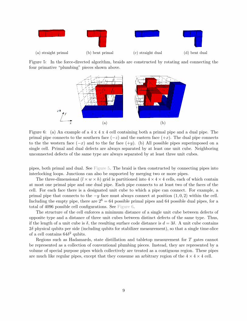
Figure 5: In the force-directed algorithm, braids are constructed by rotating and connecting thefour primative “plumbing” pieces shown above.

(a) (b)

Figure 6: (a) An example of a 4 x 4 x 4 cell containing both a primal pipe and a dual pipe. Theprimal pipe connects to the southern face (−z) and the eastern face (+x). The dual pipe connectsto the the western face (−x) and to the far face (+y). (b) All possible pipes superimposed on asingle cell. Primal and dual defects are always separated by at least one unit cube. Neighboringunconnected defects of the same type are always separated by at least three unit cubes.

pipes, both primal and dual. See Figure 5. The braid is then constructed by connecting pipes intointerlocking loops. Junctions can also be supported by merging two or more pipes.

The three-dimensional (l×w× h) grid is partitioned into 4× 4× 4 cells, each of which containat most one primal pipe and one dual pipe. Each pipe connects to at least two of the faces of thecell. For each face there is a designated unit cube to which a pipe can connect. For example, aprimal pipe that connects to the −y face must always connect at position (1, 0, 2) within the cell.Including the empty pipe, there are 26 = 64 possible primal pipes and 64 possible dual pipes, for atotal of 4096 possible cell configurations. See Figure 6.

The structure of the cell enforces a minimum distance of a single unit cube between defects ofopposite type and a distance of three unit cubes between distinct defects of the same type. Thus,if the length of a unit cube is δ, the resulting surface code distance is d = 3δ. A unit cube contains2δ physical qubits per side (including qubits for stabilizer measurement), so that a single time-sliceof a cell contains 64δ2 qubits.

Regions such as Hadamards, state distillation and tabletop measurement for T gates cannotbe represented as a collection of conventional plumbing pieces. Instead, they are represented by avolume of special purpose pipes which collectively are treated as a contiguous region. These pipesare much like regular pipes, except that they consume an arbitrary region of the 4× 4× 4 cell.

9

4.2 Braid synthesis

As defined, the braid compaction problem takes an arbitrary braid as input. Thus our algorithmneed not address the synthesis of a quantum circuit into a braid. Indeed, the force-directed braidmodel requires only that rigid collections of pipes (i.e., cuboids) be specified along with rotationand time-ordering constraints.

For concreteness, however, we will assume that the initial braid is constructed from a quantumcircuit in the canonical way as described in Section 2. That is, qubits are represented by pairs of pri-mal defects. Single-qubit preparation corresponds to two bent pipes connected to form a “U” shapeand single-qubit measurement is the same, except that the U shape is upside-down. Hadamards,state distillation and tabletop measurements are abstracted as cuboids of fixed dimension. CNOTgates are constructed by wrapping a dual loop around corresponding primal loops.

The Hadamard cuboid is three cells wide, four cells deep and four cells high. This cuboidis larger than is strictly necessary to enclose the Hadamard operation. Part of the Hadamardoperation involves cutting a boundary around the corresponding logical qubit. The volume givenabove provides enough room for the Hadamard operation to take place inside boundary, whileenforcing that defects outside of the boundary are a safe distance away. Affixed to opposite facesof the cuboid are pairs of straight pipes representing the input and output logical qubit.

The specifics of the T -gate braid depend on the distillation protocol and on the desired gateaccuracy, but otherwise follow Figure 3b. Our compaction algorithm is flexible enough to allowany type of distillation scheme. For simplicity, we will assume the existence of two cuboid regionsfor each T gate, one for |A〉 and one for |Y 〉. Straight pipes representing the output are affixed tothe top of each cuboid.

4.3 Gravity

The primary “force” in the algorithm is a vector field that loosely resembles physical gravity actingon the braid. With each cell in the grid, we associate two vectors of the form (a,m), specified byan axis a ∈ {x, y, z} and a magnitude m ∈ Z. The first vector represents a force on the primal pipecontained in the cell, and the second vector represents a force on the dual pipe.

There are a number of reasonable ways to initialize and update the gravity field as defects aremoved around. The simplest strategy is to assign a fixed, negative magnitude to each spacetimepoint and align the vector along the z-axis so that the force always points downward. In order thatdefects may slide past each other, though, we allow vectors to point sideways along the x and yaxes, as well. See Figure 7. Roughly, gravity vectors are assigned to point to the closest cell fromwhich the defect may then move downward. For example, a primal pipe occupying cell (x, y, z)may be blocked by a dual pipe in cell (x, y, z−1). If, however, cells (x+ 1, y, z) and (x+ 1, y, z−1)are empty, then the primal gravity vector for cell (x, y, z) is assigned to point along the positivex-axis.

4.4 Tension

The gravity force, while effective at directing pipes toward the bottom of the grid, has the effect ofstretching strings and loops, thus increasing the length of the the braid. This happens, for example,when a loop is pulled by gravity in one direction but a small segment of the loop is prevented frommoving because other defects are in the way. When a string or loop becomes very long, it may take

10

Figure 7: Gravity vectors (shown as green cones) generally point downward, but may point in anydirection.

(a) before (b) after

Figure 8: The tension force pulls inward on each of the corners of the loop. The result is a smallerrectangular loop.

up space that could otherwise be occupied by other parts of the braid. To prevent this behaviorwe implement a tension force which acts to reduce the length of a string.

Tension is applied to each string of defects independently. For each pipe in the string, there isa force pulling in the direction of the input face and a force pulling in the direction of the outputface. For example, a pipe connected to the −x and +z faces will experience a force in the −x and+z directions. The magnitude of the force is proportional to the length of the string, just as for aphysical spring.

This choice of tension forces means that the inward and outward forces cancel for straight pipes.Bent pipes, however, feel an inward force toward the rest of the string. This inward force tends todecrease the curvature of the string, thereby reducing its length. See Figure 8.

Tension forces also act on cuboids. Each of the pipes connected to a cuboid exerts a force thatpulls in the direction of the pipe. Again, the force is proportional to the length of the string towhich each connecting pipe belongs.

4.5 Compaction

The braid is initially placed above the three-dimensional grid. Since the braid may be wider thanthe grid dimensions, a funnel is placed on top of the grid. This allows the braid to slowly deformaccording to the geometry of the lattice. Compaction then proceeds by iterating through each ofthe cuboids and strings. Cuboids are translated or rotated as a single rigid object. Other regionsof pipes form strings which either connect to cuboids or form loops. Strings are treated as flexibleobjects in which each pipe can be translated independently.

Associated with each pipe is a velocity vector. Each pipe in a string is moved by first taking the

11

initial velocity vector and updating it according to the gravity and tension forces at that location.The pipe is then translated according to the direction and magnitude of the new velocity vector.During the move, additional pipes may be added or removed in order to maintain connectivity ofthe string.

To translate a cuboid, the total velocity is calculated by summing each of the individual velocityvectors. Similarly, the gravity and tension forces are calculated by summing the force vectorsassociated with each pipe. The cuboid velocity is then updated by dividing the total force by thenumber of pipes (each pipe is assumed to have the same mass) and then adding to the existingvelocity. Finally, the cuboid is translated according to the direction and magnitude of the velocityvector.

In the case of tabletop measurement translations along the z-axis, we must preserve the partialordering. When translating a tabletop m along the −z-axis we must check the height of the othermeasurements on which m depends. Likewise, when translating m along the +z-axis, we mustcheck the height of the measurement that depends on m.

Cuboid rotations are performed similarly by calculating a rotational velocity according to themoments of each pipe and the torque due to gravity and tension forces. Rotation about a given axisis performed only if rotation is allowed and the magnitude of the angular velocity is large enoughto induce a rotation of π/2.

Of course, all of the moves performed during compaction must maintain the braid topology. Inparticular, we do not allow pipes to intersect nor do we allow a pipe of one type to pass througha pipe of opposite type in order to arrive at its destination. Though we do allow defects of thesame type to pass through each other since this does not change the computation. It is possiblefor the translational or rotational path of a group of pipes to be blocked by other pipes. When thishappens, we say that a collision has occurred.

Collisions are resolved by first calculating the velocity and mass of each of the two objectsinvolved. In the case that a cuboid collides into multiple pipes, the impeding pipes are treated as acollective object. The velocities of the two objects are then recalculated according to the equationsof motion for a partially inelastic collision. In this way, distinct parts of the braid are able tocommunicate with each other. For example, large objects may shift smaller objects out of the wayand linked loops may tug on each other. However, the rules for moving each pipe are still entirelylocal and relatively simple.

Note that a collision can also occur between time-dependent measurements even when the twocuboids are not located nearby each other. Such a collision happens if the vertical motion of oneof the measurements would cause a violation of relative time-ordering constraints. The collision isnon-local, but can be efficiently identified and resolved by maintaining a dependency tree with thelocation of measurement.

Since the topology of the braid is preserved at each step, compaction can be terminated atany time. Indeed, there are a number of reasonable termination conditions. Compaction can bestopped after a fixed number of iterations, or a fixed amount of time. It can also be stopped whenall of the pipes are located below a particular height, or as soon as all of the pipes fit within thedimensions of the lattice. The termination condition could also be more complicated. For example,compaction could be halted if the maximum height remains unchanged for a certain fixed numberof iterations.

12

4.6 Performance and scalability

The complexity of a single compaction iteration scales as the size of the braid. The size of acanonical braid is O(nm) where n is the number of qubits and m is the number of gates in theinput circuit. The number of iterations required to obtain good compaction results depends onthe ratio of the lattice area—i.e., the x-y plane—to the braid size. In the case that the latticearea is large compared to the braid size, it seems reasonable to expect the braid to flatten in timeproportional to the height of the canonical braid. If the canonical braid has area large comparedto the lattice, then O(nm) iterations may be required in order to funnel then entire braid into theproper bounding box.

For small circuit sizes, a runtime of O(n2m2) is reasonable. But for large circuits consisting ofthousands of qubits and possibly millions or billions of gates, we require a better strategy. Indeed,we cannot hope to globally optimize braids for large-scale problem sizes. Instead, the circuitis partitioned into subcircuits of manageable size and the braid is synthesized and compactedhierarchically. Just as we treat single-qubit Hadamards as atomic cuboids of fixed size, we mayconsider sub-braids as fixed size cuboids.

Each sub-braid is represented as a tangle of defects in which some defects are anchored to gridboundaries. Subject to the anchoring constraints, the sub-braid is compacted as normal. Once itscompacted size is determined, the sub-braid is then treated as a black-box in the larger braid. Iftwo sub-braids contain measurements that are time-ordered, then the sub-braids must also be timeordered. But again, this is no different than time ordering restrictions on tabletop measurementsin the original model.

We anticipate that the best partitioning strategy will be one that reflects the structure of theinput circuit. Reasonable representations of large input circuits will be hierarchical and it shouldbe possible to mimic this hierarchy for large-scale compaction. This technique will be particularlyuseful for highly repetitive circuits. Repeated sub-circuits can be synthesized and compacted once,and then duplicated in the larger braid.

4.7 Implementation and results

We have implemented the force-directed compaction algorithm in C++ as a tool called Braidpack.Braidpack takes, as input, a representation of a circuit along with physical space restrictions. Itproduces, as output, a compact logically equivalent surface code braid.

The current implementation is not yet fully functional, but is capable of synthesizing and com-pacting arbitrary circuits of CNOT gates, including qubit preparation and measurement. Figure 9shows the result of compaction on a single CNOT gate. The tension force first contracts the primalloop on the right-hand-side. Then gravity flattens the braid. Compaction in this example was donewithout implementing collisions between pipes. As a result, tension is unable to fully contract thedual loop. Once implementation is complete, we expect the braid to fully flatten and contract.

Figure 10 shows the same prototype implementation of Braidpack for a circuit composed ofeleven CNOT gates. For simplicity of implementation, the qubit preparation and measurements inthe canonical braid are arranged in a staircase fashion. Ignoring the staircases, the canonical braidhas a bounding box of size (3× 16× 34), whereas the the compacted braid fits in a bounding boxof size (10× 13× 6), a factor of four improvement along the time axis. Again, we expect improvedresults once the Braidpack completed.

In order to facilitate debugging, we have developed a braid visualization tool called Braid-

13

(a) (b)

Figure 9: Compaction of a single CNOT using a prototype of the force-directed algorithm. (a)A canonical CNOT braid is initially arranged vertically. (b) After compaction, the braid has beenalmost completely flattened.

view. This tool creates a single file from a braid or sequence of braids. The file can be viewedin Blender [Ble], a third-party open-source 3-D modeling application. Braidview is capable ofseparately rendering primal and dual defects (as in Figure 10), as well as gravity vectors (see Fig-ure 7). The backbone of Braidview is a set of rendering functions that use the Blender Python-API.These, and some additional functions, are used by similar visualization tools Nestcheck and Auto-tune [MF12, FWMR12].

5 Compaction by simulated annealing

In this section we describe our second compaction algorithm, which is based on simulated annealing.Simulated annealing is a general optimization technique that has been applied to a wide variety ofproblems. The main idea is to explore the solution space by hopping randomly from the currentsolution to a nearby solution. Hops that result in an improved solution are kept. In order toavoid local minima, hops that result in a less desirable solution are also kept with some non-zeroprobability, thus permitting broader exploration of the set of possible solutions.

Our simulated annealing algorithm is based largely on a procedure used for VLSI placement[HLL88]. In the VLSI algorithm, circuit elements and wires are represented by rectangles. Size,distance and connectivity constraints are given by linear inequalities on the coordinates of eachrectangle. Rectangles can be shifted around by swapping linear constraints. The idea for braids issimilar. Defects are represented by cuboids. Size, distance and topology constraints are given bylinear inequalities which can be swapped to perform topological deformation.

5.1 Definition of the braid

In the force-directed algorithm, the braid was modeled as a connected configuration of plumbingpieces. Some collections of pipes formed rigid cuboids. Other collections of pipes formed flexiblestrings and loops. For simulated annealing, we take a different approach. Each cuboid is representedby a pair of points (p, p′) in the three-dimensional lattice. Point p specifies the point closest to theorigin (lower-left corner) and p′ specifies the point furthest from the origin (upper-right corner).Defect strings and loops are also represented by cuboids. A string of defects is given by a set ofoverlapping cuboids of arbitrary dimension. By connecting cuboids it is possible to construct any

14

(a) (b)

Figure 10: Compaction of eleven CNOT gates with a prototype implementation of the force-directed algorithm. The canonical braid (a) is compressed into a smaller but topologically equivalentbraid (b).

15

desired loop or string.Thus the entire braid is specified by a set of cuboids. A layout of n cuboids is defined by 2n

three-dimensional integer coordinates. The x, y, z dimensions of the layout are defined by themaximum x, y, and z coordinates respectively. The layout must satisfy a set of constraints whichwe group the constraints into the following types:

1. size constraints,

2. time-ordering constraints,

3. minimum distance constraints,

4. jog constraints,

5. connectivity constraints and

6. topological constraints.

Except for the topological constraints, all of the constraints can be directly expressed as sets oflinear inequalities.

5.1.1 Size constraints

Minimum dimension constraints of a cuboid are specified by a triple (δx, δy, δz) of non-negative realvalues and three linear inequalities:

x+ δx ≤ x′y + δy ≤ y′z + δz ≤ z′ .

(1)

For string cuboids (those that are not H gates or table-like measurements), δx = δy = δz = d/4,where d is the code distance. Hadamard and T gates may be rotated 90 degrees about the z-axis. Each gate can take on one of four different rotations {0, π/2, π,−π/2}. Rotations 0 and πcorrespond to the set of constraints given by (1). Rotations ±π/2 correspond to the same set ofconstraints in which δx and δy have been exchanged.

We therefore assign one of two sets of constraints to each H and T gate, either the constraintsof (1) or the permuted version. The corresponding cuboids must satisfy all constraints from atleast one of sets.

5.1.2 Time-ordering constraints

The non-deterministic implementation of T gates in the surface code induces a partial time-orderingof tabletop measurement regions. As discussed in Section 2, this partial ordering requires that, forcertain pairs, one tabletop measurement must be located above another tabletop measurement.The time-ordering constraint for two dependent measurements, a, b is given by,

z′a + 1 ≤ zb . (2)

16

5.1.3 Minimum distance constraints

Like the size constraints, minimum distances are proportional to d, the distance of the code. Witha few exceptions (see Section 5.1.4 and Section 5.1.5), primal defect cuboids must be at least adistance d away from other primal defects. Similarly, dual defect cuboids must be d away fromother dual cuboids. Cuboids of opposite type must be at least d/4 apart.

If two cuboids ri, rj must be separated by δ, then at least one of the following constraints mustbe satisfied:

x′i + δ ≤ xj x′j + δ ≤ xiy′i + δ ≤ yj y′j + δ ≤ yiz′i + δ ≤ zj z′j + δ ≤ zi

(3)

Each constraint corresponds to a different relative arrangement of the two cuboids. The x′i+δ ≤ xjconstraint, for example, enforces that ri is placed to the left of rj . Whereas z′i + δ ≤ zj requiresthat ri be placed below rj .

5.1.4 Jog nodes

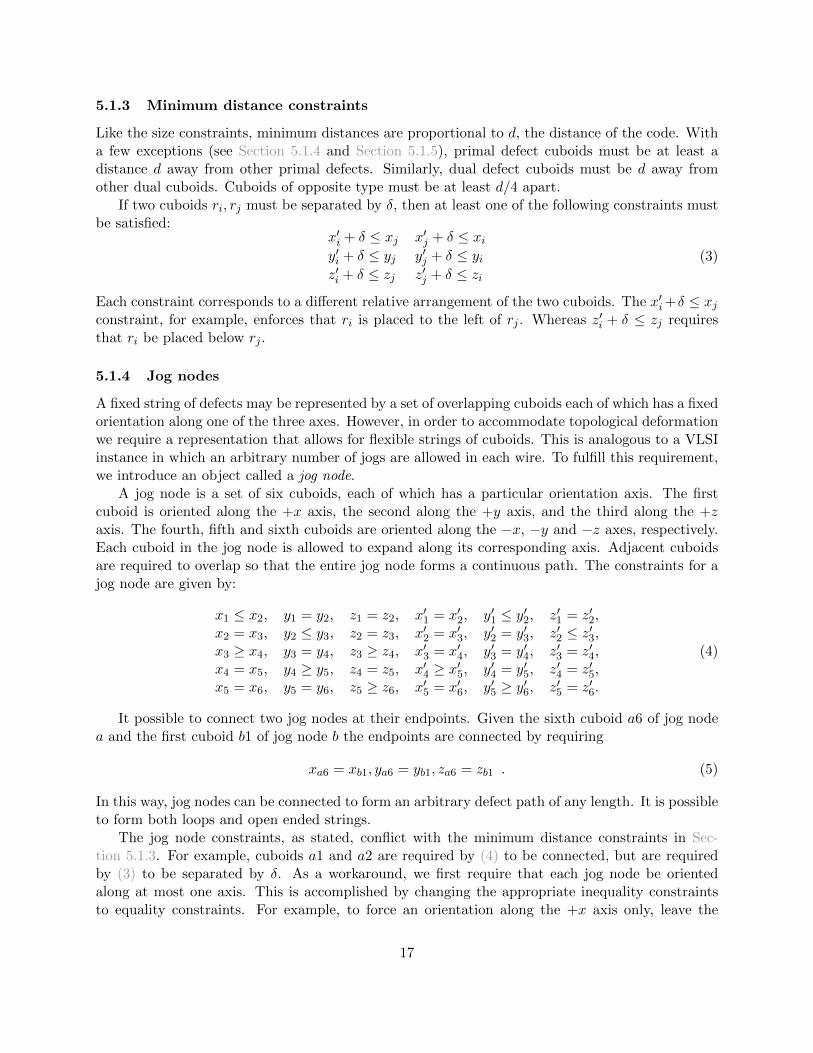
A fixed string of defects may be represented by a set of overlapping cuboids each of which has a fixedorientation along one of the three axes. However, in order to accommodate topological deformationwe require a representation that allows for flexible strings of cuboids. This is analogous to a VLSIinstance in which an arbitrary number of jogs are allowed in each wire. To fulfill this requirement,we introduce an object called a jog node.

A jog node is a set of six cuboids, each of which has a particular orientation axis. The firstcuboid is oriented along the +x axis, the second along the +y axis, and the third along the +zaxis. The fourth, fifth and sixth cuboids are oriented along the −x, −y and −z axes, respectively.Each cuboid in the jog node is allowed to expand along its corresponding axis. Adjacent cuboidsare required to overlap so that the entire jog node forms a continuous path. The constraints for ajog node are given by:

x1 ≤ x2, y1 = y2, z1 = z2, x′1 = x′2, y′1 ≤ y′2, z′1 = z′2,x2 = x3, y2 ≤ y3, z2 = z3, x′2 = x′3, y′2 = y′3, z′2 ≤ z′3,x3 ≥ x4, y3 = y4, z3 ≥ z4, x′3 = x′4, y′3 = y′4, z′3 = z′4,x4 = x5, y4 ≥ y5, z4 = z5, x′4 ≥ x′5, y′4 = y′5, z′4 = z′5,x5 = x6, y5 = y6, z5 ≥ z6, x′5 = x′6, y′5 ≥ y′6, z′5 = z′6.

(4)

It possible to connect two jog nodes at their endpoints. Given the sixth cuboid a6 of jog nodea and the first cuboid b1 of jog node b the endpoints are connected by requiring

xa6 = xb1, ya6 = yb1, za6 = zb1 . (5)

In this way, jog nodes can be connected to form an arbitrary defect path of any length. It is possibleto form both loops and open ended strings.

The jog node constraints, as stated, conflict with the minimum distance constraints in Sec-tion 5.1.3. For example, cuboids a1 and a2 are required by (4) to be connected, but are requiredby (3) to be separated by δ. As a workaround, we first require that each jog node be orientedalong at most one axis. This is accomplished by changing the appropriate inequality constraintsto equality constraints. For example, to force an orientation along the +x axis only, leave the

17

Figure 11: A jog node consists of six overlapping cuboids. Each cuboid is allowed to extend inonly one direction, and only one cuboid in the node may be extended. The six possible jog nodeconfigurations are shown above. The node origin is indicated by a black dot, where visible.

x1 ≤ x2 constraint alone and change all of the other inequalities to equalities. Then the cuboidcorresponding to the +x axis can be of arbitrary size (subject to minimum dimension constraints)and all other cuboids of the node must fit inside of it. See Figure 11.

Next, remove the minimum distance constraints for all jog node cuboids except those thatcorrespond to the orientation axis. Finally, remove minimum distance constraints between cuboidsin adjacent jog nodes. Now, overlapping cuboids within the same jog node or between connectedjog nodes are consistent with all other constraints.

A jog node may also be configured to take no orientation. In this case, all cuboids in the nodeare constrained to be of minimum size, i.e., x + δx = x′, y + δy = y′, z + δz = z′. Furthermore,all minimum distance constraints involving the node are removed. This type of node will either beunconnected to any other node (in which case it can be removed), or it will be contained entirelywithin another jog node. In either case, its distance from other objects in the braid is unimportant.

5.1.5 Connectivity constraints

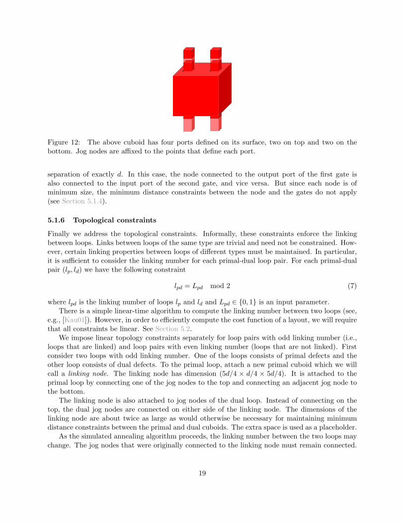
Jog nodes allow for arbitrary defect paths and loops. We must also define how jog nodes are used toconnect to cuboids such as Hadamard gates and state distillation. Each gate cuboid contains somenumber of ports to which string defect cuboids are allowed to attach. The locations of the portsare fixed relative to the gate. However, since gates can be rotated, the constraints that describe theconnection must correspond to the permutation of the dimensional constraints from Section 5.1.1.

A port is a rectangle defined by two coordinates on the surface of the gate. A jog node is con-nected to a port by requiring that certain coordinates of the jog node cuboid match the coordinatesof the port. For example, if the input port (x, y, z), (x′, y′, z) is located on the top of the gate, thenthe jog node connection constraint is given by

x3 = x, y3 = y, x′3 = x′, y′3 = y′, z3 = z . (6)

See Figure 12.To maintain consistency, the minimum distance constraints between the gate and the connecting

jog node must be eliminated. Note that it is still possible for two connected gates to achieve a

18

Figure 12: The above cuboid has four ports defined on its surface, two on top and two on thebottom. Jog nodes are affixed to the points that define each port.

separation of exactly d. In this case, the node connected to the output port of the first gate isalso connected to the input port of the second gate, and vice versa. But since each node is ofminimum size, the minimum distance constraints between the node and the gates do not apply(see Section 5.1.4).

5.1.6 Topological constraints

Finally we address the topological constraints. Informally, these constraints enforce the linkingbetween loops. Links between loops of the same type are trivial and need not be constrained. How-ever, certain linking properties between loops of different types must be maintained. In particular,it is sufficient to consider the linking number for each primal-dual loop pair. For each primal-dualpair (lp, ld) we have the following constraint

lpd = Lpd mod 2 (7)

where lpd is the linking number of loops lp and ld and Lpd ∈ {0, 1} is an input parameter.There is a simple linear-time algorithm to compute the linking number between two loops (see,

e.g., [Kau01]). However, in order to efficiently compute the cost function of a layout, we will requirethat all constraints be linear. See Section 5.2.

We impose linear topology constraints separately for loop pairs with odd linking number (i.e.,loops that are linked) and loop pairs with even linking number (loops that are not linked). Firstconsider two loops with odd linking number. One of the loops consists of primal defects and theother loop consists of dual defects. To the primal loop, attach a new primal cuboid which we willcall a linking node. The linking node has dimension (5d/4 × d/4 × 5d/4). It is attached to theprimal loop by connecting one of the jog nodes to the top and connecting an adjacent jog node tothe bottom.

The linking node is also attached to jog nodes of the dual loop. Instead of connecting on thetop, the dual jog nodes are connected on either side of the linking node. The dimensions of thelinking node are about twice as large as would otherwise be necessary for maintaining minimumdistance constraints between the primal and dual cuboids. The extra space is used as a placeholder.

As the simulated annealing algorithm proceeds, the linking number between the two loops maychange. The jog nodes that were originally connected to the linking node must remain connected.

19

(a) (b) (c)

Figure 13: When a primal and a dual loop are linked in the canonical braid a linking node (a) isinserted and attached to both loops. Once compaction has completed, the linking node is removed.The linking number can be left unchanged (b), or toggled (c) if necessary.

Figure 14: In order to avoid unwanted links, a cuboid is placed around each primal loop. Dualloops which do not link with the primal loop are prohibited from entering the enclosing cuboid.

But other cuboids from the loops are unrestricted and may cross each other. At the end of thealgorithm the linking node is removed leaving some empty space.

The primal and dual loops must now be reconnected. However, we have a choice. We may eitherconnect the dual loop so that it is inside of the primal loop. Or we may connect the dual loop sothat it is outside of the primal loop. In effect, the choice of reconnection determines whether thelinking number is even or odd. We may simply choose the configuration that yields an odd linkingnumber. See Figure 13.

Now consider a primal loop and a dual loop with even linking number. Since these loops areunlinked, they may be far apart in spacetime. Thus the linking node strategy is not practical.However, we must still ensure that these loops remain unlinked in the output of the algorithm. Wewill do this by requiring that the dual loop remain sufficiently far from the primal loop at all times.

Consider the primal loop. It is composed of a set of connected primal cuboids, some of whichare jog nodes and some of which are Hadamard or state distillation cuboids. Let x be the minimalx-coordinate of any cuboid in this set and let x′ be the maximal x-coordinate of any cuboid in theset. Similarly define y, y′, z and z′ as the minimal and maximal y- and z-coordinates. Then theentire primal loop is contained in a bounding box of dimension (x′ − x, y′ − y, z′ − z).

If all of the cuboids in the dual loop stay outside of the bounding box that encloses the primalloop, then the linking number is guaranteed to be zero. We therefore introduce a new cuboid thatencloses the primal loop. For all dual loops which have even linking number with the correspondingprimal loop, we add primal-dual minimum distance constraints between the dual cuboids and theenclosing cuboid. See Figure 14.

In order to ensure that the new cuboid actually encloses the primal loop, additional variables andconstraints are required. Let (x, y, z) and (x′, y′, z′) be variables describing the enclosing cuboid.

20

Then for each cuboid (xi, yi, zi), (x′i, y′i, z

′i) in the primal loop we require that

x ≤ xi x′i ≤ x′y ≤ yi y′i ≤ y′z ≤ zi z′i ≤ z′.

(8)

5.2 The annealing algorithm

The algorithm takes a canonical braid as input. Initialization consists of constructing all of thecuboids and constraint groups. The instance includes a set of coordinates P , which can be dividedinto sets of integers X, Y and Z corresponding to the x-, y−, and z-coordinates, respectively.The constraints can be represented as a set C of integer triples. Some of the constraints, suchat time-ordering constraints, must be satisfied for all possible layouts. Other constraints may bepartitioned into subsets for which the layout must satisfy at least one of the constraints in thesubset. Let C ′ be the set of all constraints that must always be satisfied, let C ′′ be the remainingconstraints and let B be the corresponding partition into constraint subsets. Let A ⊂ C be the setof “active” constraints such that C ′ ⊂ A and A contains exactly one constraint from each elementof B.

Start by choosing a set of active constraints such that all constraints in A are satisfied by thecanonical braid. The algorithm then proceeds by repeating the following sequence.

1. Randomly select an element β ∈ B.

2. Randomly select a constraint b ∈ β such that b 6∈ A.

3. Locate the single constraint in b′ ∈ A ∩ β. Remove b′ from A and replace it with the newconstraint b.

4. Compute the new minimum bounding box size and corresponding cost function.

5. If the new set of active constraints is infeasible, then reject the swap by removing b from Aand replacing with b′.

6. If the cost is smaller than before, keep the new constraint.

7. If the cost is larger than before, then keep the new constraint with probability given by theannealing schedule (see below).

In order for the algorithm to be efficient, we require an efficient way to compute the size of theminimum bounding box. This can be done using the constraint graph method proposed in [LW83]and used by [HLL88]. First, partition the active constraints into three sets: those that involveonly x coordinates, those that involve only y coordinates and those that involve only z coordinates.Note that there are no constraints that involve coordinates for two different axes. Consider justthe set of x-coordinates X. We construct a weighted directed graph GX = (VX , EX). AssignVX = X ∪{x∅, x∞} where x∅ and x∞ are a boundary coordinates. For each constraint xi ≤ xj +dijthere is a directed edge from vertex xi to vertex xj with weight dij . The value of each coordinatex ∈ X is assigned by computing the longest path from x∅ to x. Assuming that the set of constraintscan be satisfied, GX is a acyclic. Thus the longest path can be computed in linear time by negating

21

the weights and using Dijkstra’s algorithm. Constraint graphs for y and z coordinates are similarlyconstructed.

The cost of constructing the initial constraint graphs is O(n2), where n is the number of cuboids.Once the graphs are constructed, updates can be computed by an online algorithm. When aconstraint swap is performed, only those paths affected by the corresponding vertices need to berecalculated. This algorithm can also detect cycles induced by the new constraint. If a cycle isdetected, then the set of constraints is infeasible and the swap is rejected.

There are a number of choices of cost function. The goal is to construct a braid of small heightthat fits into an x-y area of fixed size. The first step is to ensure that the braid fits into that area.We initially set the cost function as the x-coordinate of the bounding box. Once this x-coordinateis small enough, we impose a global constraint that the x-coordinates of all cuboids must be nogreater than that of the bounding box. We then set the cost function as the y-coordinate of thebounding box and repeat the procedure. Finally, once the entire braid fits into the x-y area, weminimize over the height.

For VLSI placement Hsieh, Leong and Liu use a fixed-ratio temperature schedule in which thetemperature is reduced by a constant factor after each time step. This schedule is simple andefficient and can also be used for our algorithm. Other kinds of schedules could also be used.

6 Discussion and future work

The surface code provides a unique opportunity for fault-tolerant quantum circuit optimization bytopological deformation. We have defined the problem of braid compaction subject to geometricconstraints, and given two heuristic algorithms. Our tool Braidpack implements the first of these,the force-directed algorithm. Small examples indicate that compaction algorithms can lead tosignificant improvement in spacetime overhead when compared to the canonical braid.

Braidpack is a work in progress, and we intend implement all of the features outlined in Section 4and to scale up the size of the input examples. We would also like to implement the simulatedannealing algorithm in order to compare the performance of the two algorithms. Indeed, we couldalso construct a hybrid algorithm which incorporates both techniques.

Our simulated annealing algorithm is inspired from a similar algorithm for VLSI placement.VLSI also offers a number of other techniques including, genetic algorithms, numerical and parti-tioning algorithms, and force-directed algorithms that are distinct from our own (see, e.g., [SM91]).Perhaps some of these additional techinques could be adapted to braid compaction.

Due to similarity with VLSI compaction and other packing problems, we conjecture that braidcompaction is NP-complete. A formal reduction has proven elusive, however. Thus an obviousopen problem is to confirm or refute that conjecture.

Finally, we have focused on topological deformation. However, other non-topological braididentities exist [FD12, RHG07]. Optimization involving these identities has been previously doneby hand, but it may be possible to incorporate non-topological techniques into an automated toolsuch as ours.

Acknowledgements

AEP would like to thank Lucy Zhang and Vinayak Pathak for insightful discussions regarding com-plexity of braid compaction. Thanks also to Andrew Kennings for consultation on VLSI placement

22

algorithms.Supported by the Intelligence Advanced Research Projects Activity (IARPA) via Department of

Interior National Business Center contract number D11PC20166. The U.S. Government is autho-rized to reproduce and distribute reprints for Governmental purposes notwithstanding any copyrightannotation thereon. Disclaimer: The views and conclusions contained herein are those of the au-thors and should not be interpreted as necessarily representing the official policies or endorsements,either expressed or implied, of IARPA, DoI/NBC, or the U.S. Government.

References

[AUW+10] J M Amini, H Uys, J H Wesenberg, S Seidelin, J Britton, J J Bollinger, D Leibfried,C Ospelkaus, A P VanDevender, and D J Wineland. Scalable ion traps for quantuminformation processing. New J. Phys., 12:33031, 2010.

[BH12] Sergey Bravyi and Jeongwan Haah. Magic-state distillation with low overhead. Phys.Rev. A, 86(5):052329, September 2012, arXiv:1209.2426.

[BK04] Sergey Bravyi and Alexei Kitaev. Universal quantum computation with ideal Cliffordgates and noisy ancillas. Phys. Rev. A, 71(2):022316, February 2004, arXiv:0403025.

[BK09] Anne Broadbent and Elham Kashefi. Parallelizing quantum circuits. Theoretical Com-puter Science, 2009, arXiv:0704.1736.

[Ble] Blender, http://www.blender.org.

[CDKM04] SA A Cuccaro, TG G Draper, S A Kutin, and D P Moulton. A new quantum ripple-carry addition circuit. October 2004, arXiv:0410184.

[CW00] Richard Cleve and John Watrous. Fast parallel circuits for the quantum Fouriertransform. Foundations of Computer Science, 2000. . . . , pages 526–536, June 2000,arXiv:0006004.

[DFS+09] S J Devitt, Austin G. Fowler, A M Stephens, A D Greentree, Lloyd C. L. Hollenberg,W J Munro, and Kae Nemoto. Architectural design for a topological cluster statequantum computer. New. J. Phys., 11:83032, 2009.

[DiV09] David P. DiVincenzo. Fault-tolerant architectures for superconducting qubits. PhysicaScripta, T137(T137):014020, December 2009.

[dSPK13] Raphael Dias da Silva, Einar Pius, and Elham Kashefi. Global Quantum CircuitOptimization. January 2013, arXiv:1301.0351.

[FD12] Austin G. Fowler and Simon J. Devitt. A bridge to lower overhead quantum compu-tation. arXiv:1209.0510, September 2012, arXiv:1209.0510.

[FDJ13] Austin G. Fowler, Simon J. Devitt, and N. Cody Jones. Surface code implementationof block code state distillation. January 2013, arXiv:1301.7107.

23

[FMMC12] Austin G. Fowler, Matteo Mariantoni, John M. Martinis, and Andrew N. Cleland. Aprimer on surface codes: Developing a machine language for a quantum computer.August 2012, arXiv:1208.0928.

[Fow12a] Austin G. Fowler. Low-overhead surface code logical H. February 2012,arXiv:1202.2639.

[Fow12b] Austin G. Fowler. Time-optimal quantum computation. October 2012,arXiv:1210.4626.

[FWMR12] Austin G. Fowler, Adam C. Whiteside, Angus L. McInnes, and Alimohammad Rab-bani. Topological code Autotune. February 2012, arXiv:1202.6111.

[GFG12] Joydip Ghosh, Austin G. Fowler, and MR Geller. Surface code with decoherence: Ananalysis of three superconducting architectures. Physical Review A, October 2012,arXiv:1210.5799.

[HLL88] T.M. Hsieh, H.W. Leong, and C.L. Liu. Two-dimensional layout compaction by sim-ulated annealing. In IEEE International Symposium on Circuits and Systems, pages2439–2443. IEEE, 1988.

[HMF+09] F. Helmer, Matteo Mariantoni, Austin G. Fowler, J. von Delft, E. Solano, and F. Mar-quardt. Cavity grid for scalable quantum computation with superconducting circuits.EPL (Europhysics Letters), 85(5):50007, March 2009.

[Jon12] N. Cody Jones. Multilevel distillation of magic states for quantum computing. October2012, arXiv:1210.3388.

[JVF+12] N. Cody Jones, Rodney Van Meter, Austin G. Fowler, Peter L McMahon, JungsangKim, Thaddeus D Ladd, and Yoshihisa Yamamoto. Layered Architecture for QuantumComputing. Physical Review X, 2(3):031007, July 2012.

[Kau01] LH Kauffman. Knots and physics. World Scientific, Teaneck, NJ, 2001.

[KBB11] M Kumph, M Brownnutt, and R Blatt. Two-Dimensional Arrays of RF Ion Traps withAddressable Interactions. New J. Phys., 13:73043, 2011.

[KL13] Christoph Kloeffel and Daniel Loss. Prospects for Spin-Based Quantum Computing inQuantum Dots. Annual Review of Condensed Matter Physics, 4(1):51–81, April 2013.

[Kni05] Emanuel Knill. Quantum Computing with Very Noisy Devices. Nature, 434(7029):39–44, 2005, arXiv:0410199.

[Kob12] Stephen G. Kobourov. Spring Embedders and Force Directed Graph Drawing Algo-rithms. page 23, January 2012, arXiv:1201.3011.

[LCG+11] James E Levy, Malcolm S Carroll, Anand Ganti, Cynthia A Phillips, Andrew J. Lan-dahl, Thomas M Gurrieri, Robert D Carr, Harold L Stalford, and Erik Nielsen. Impli-cations of electronics constraints for solid-state quantum error correction and quantumcircuit failure probability. New Journal of Physics, 13(8):083021, August 2011.

24

[Lev01] Jeremy Levy. Quantum-information processing with ferroelectrically coupled quantumdots. Physical Review A, 64(5):052306, October 2001.

[LW83] Y.Z. Liao and C.K. Wong. An Algorithm to Compact a VLSI Symbolic Layout withMixed Constraints. In 20th Design Automation Conference Proceedings, pages 107–112.IEEE, 1983.

[MDMN08] Dmitri Maslov, G.W. Dueck, D.M. Miller, and C. Negrevergne. Quantum CircuitSimplification and Level Compaction. IEEE Transactions on Computer-Aided Designof Integrated Circuits and Systems, 27(3):436–444, March 2008, arXiv:0604001.

[MEK13] Adam M. Meier, Bryan Eastin, and Emanuel Knill. Magic-state distillation with thefour-qubit code. Quant. Inf. Comput., 13(3&4):195–209, April 2013, arXiv:1204.4221.

[MF12] Thomas J. Milburn and Austin G. Fowler. Checking the error correction strength ofarbitrary surface code logical gates. October 2012, arXiv:1210.4249.

[MN01] Cristopher Moore and Martin Nilsson. Parallel quantum computation and quantumcodes. SIAM Journal on Computing, 2001.

[PR12] Adam Paetznick and Ben W. Reichardt. Fault-tolerant ancilla preparation andnoise threshold lower bounds for the 23-qubit Golay code. Quant. Inf. Comput.,12(11&12):1034–1080, November 2012, arXiv:1106.2190.

[RB01] Robert Raussendorf and Hans Briegel. Computational model underlying the one-wayquantum computer. arXiv preprint quant-ph/0108067, August 2001, arXiv:0108067.

[Rei06] Ben W. Reichardt. Error-detection-based quantum fault tolerance against discrete Paulinoise. PhD thesis, UC Berkeley, 2006.

[RH07] Robert Raussendorf and Jim Harrington. Fault-Tolerant Quantum Computation withHigh Threshold in Two Dimensions. Phys. Rev. Lett., 98(19):190504, May 2007,arXiv:0610082.

[RHG07] Robert Raussendorf, J Harrington, and Krittika Goyal. Topological fault-tolerance incluster state quantum computation. New Journal of Physics, 9(6):199–199, June 2007,arXiv:0703143.

[Sch92] Guntram Scheithauer. Algorithms for the container loading problem. Operations Re-search, 445, 1992.

[Sho96] Peter W. Shor. Fault-tolerant quantum computation. Proc. 37th Annual Symp. onFoundations of Computer Science (FOCS), pages 56–65, 1996, arXiv:9605011.

[SLW83] M. Schlag, Y.-Z. Liao, and C.K. Wong. An algorithm for optimal two-dimensionalcompaction of VLSI layouts. Integration, the VLSI Journal, 1(2-3):179–209, October1983.

[SM91] K. Shahookar and P. Mazumder. VLSI cell placement techniques. ACM ComputingSurveys, 23(2):143–220, June 1991.

25

[Ste04] Andrew M. Steane. Fast fault-tolerant filtering of quantum codewords. 2004,arXiv:0202036.

[SWD10] Mehdi Saeedi, Robert Wille, and Rolf Drechsler. Synthesis of quantum circuits forlinear nearest neighbor architectures. Quantum Information Processing, 10(3):355–377, October 2010, arXiv:1110.6412.

[WHL05] Yaakov Weinstein, C. Hellberg, and Jeremy Levy. Quantum-dot cluster-state comput-ing with encoded qubits. Physical Review A, 72(2):020304, August 2005.

26