374
Quantum field theory: Lecture Notes Rodolfo Alexander Diaz Sanchez Universidad Nacional de Colombia Departamento de F´ ısica Bogot´ a, Colombia August 23, 2015

Quantum field theory: Lecture Notes
Rodolfo Alexander Diaz SanchezUniversidad Nacional de Colombia
Departamento de FısicaBogota, Colombia
August 23, 2015

Contents
1 Relativistic quantum mechanics 7
1.1 Survey on quantum mechanics . . . . . . . . . . . . . . . . . . . . . . . . . . . . . . . . . . . . . . 7
1.1.1 Vector subspaces generated by eigenvalues . . . . . . . . . . . . . . . . . . . . . . . . . . . . 8
1.2 Symmetries in quantum mechanics . . . . . . . . . . . . . . . . . . . . . . . . . . . . . . . . . . . . 9
1.3 Irreducible inequivalent representations of groups . . . . . . . . . . . . . . . . . . . . . . . . . . . . 12
1.4 Connected Lie groups . . . . . . . . . . . . . . . . . . . . . . . . . . . . . . . . . . . . . . . . . . . 14
1.5 Lorentz transformations . . . . . . . . . . . . . . . . . . . . . . . . . . . . . . . . . . . . . . . . . . 17
1.6 The inhomogeneous Lorentz Group (or Poincare group) . . . . . . . . . . . . . . . . . . . . . . . . 19
1.6.1 Four-vectors and tensors . . . . . . . . . . . . . . . . . . . . . . . . . . . . . . . . . . . . . . 20
1.7 Some subgroups of the Poincare group . . . . . . . . . . . . . . . . . . . . . . . . . . . . . . . . . . 22
1.7.1 Proper orthochronous Lorentz group . . . . . . . . . . . . . . . . . . . . . . . . . . . . . . . 23
1.7.2 Discrete transformations in the Lorentz group . . . . . . . . . . . . . . . . . . . . . . . . . . 24
1.7.3 Infinitesimal transformations within the proper orthochronus Lorentz group . . . . . . . . . 25
1.8 Quantum Lorentz Transformations . . . . . . . . . . . . . . . . . . . . . . . . . . . . . . . . . . . . 25
1.8.1 Four-vector and tensor operators . . . . . . . . . . . . . . . . . . . . . . . . . . . . . . . . . 26
1.8.2 Infinitesimal quantum Lorentz transformations . . . . . . . . . . . . . . . . . . . . . . . . . 27
1.8.3 Lorentz transformations of the generators . . . . . . . . . . . . . . . . . . . . . . . . . . . . 28
1.8.4 Lie algebra of the Poincare generators . . . . . . . . . . . . . . . . . . . . . . . . . . . . . . 29
1.8.5 Physical interpretation of Poincare’s generators . . . . . . . . . . . . . . . . . . . . . . . . . 30
1.9 One-particle states . . . . . . . . . . . . . . . . . . . . . . . . . . . . . . . . . . . . . . . . . . . . . 32
1.9.1 One-particle states under pure translations . . . . . . . . . . . . . . . . . . . . . . . . . . . 32
1.9.2 One-particle states under homogeneous Lorentz transformations . . . . . . . . . . . . . . . 32
1.9.3 Physical little groups . . . . . . . . . . . . . . . . . . . . . . . . . . . . . . . . . . . . . . . . 35
1.9.4 Normalization of one-particle states . . . . . . . . . . . . . . . . . . . . . . . . . . . . . . . 36
1.10 One-particle states with non-null mass . . . . . . . . . . . . . . . . . . . . . . . . . . . . . . . . . . 38
1.10.1 Wigner rotation and standard boost . . . . . . . . . . . . . . . . . . . . . . . . . . . . . . . 40
1.11 One-particle states with null mass . . . . . . . . . . . . . . . . . . . . . . . . . . . . . . . . . . . . 44
1.11.1 Determination of the little group . . . . . . . . . . . . . . . . . . . . . . . . . . . . . . . . . 44
1.11.2 Lie algebra of the little group ISO (2) . . . . . . . . . . . . . . . . . . . . . . . . . . . . . . 48
1.11.3 Massless states in terms of eigenvalues of the generators of ISO (2) . . . . . . . . . . . . . . 50
1.11.4 Lorentz transformations of massless states . . . . . . . . . . . . . . . . . . . . . . . . . . . . 51
1.12 Space inversion and time-reversal . . . . . . . . . . . . . . . . . . . . . . . . . . . . . . . . . . . . . 53
1.13 Parity and time-reversal for one-particle states with M > 0. . . . . . . . . . . . . . . . . . . . . . . 56
1.13.1 Parity for M > 0 . . . . . . . . . . . . . . . . . . . . . . . . . . . . . . . . . . . . . . . . . . 56
1.13.2 Time reversal for M > 0 . . . . . . . . . . . . . . . . . . . . . . . . . . . . . . . . . . . . . . 58
1.13.3 Parity for null mass particles . . . . . . . . . . . . . . . . . . . . . . . . . . . . . . . . . . . 59
1.13.4 Time-reversal for null mass particles . . . . . . . . . . . . . . . . . . . . . . . . . . . . . . . 62
1.14 Action of T 2 and Kramer’s degeneracy . . . . . . . . . . . . . . . . . . . . . . . . . . . . . . . . . . 63
2

CONTENTS 3
2 Scattering theory 65
2.1 Construction of “in” and “out” states . . . . . . . . . . . . . . . . . . . . . . . . . . . . . . . . . . 65
2.2 The S−matrix . . . . . . . . . . . . . . . . . . . . . . . . . . . . . . . . . . . . . . . . . . . . . . . 70
2.3 Symmetries of the S−matrix . . . . . . . . . . . . . . . . . . . . . . . . . . . . . . . . . . . . . . . 75
2.3.1 Lorentz invariance . . . . . . . . . . . . . . . . . . . . . . . . . . . . . . . . . . . . . . . . . 75
2.3.2 Internal symmetries . . . . . . . . . . . . . . . . . . . . . . . . . . . . . . . . . . . . . . . . 81
2.3.3 Parity . . . . . . . . . . . . . . . . . . . . . . . . . . . . . . . . . . . . . . . . . . . . . . . . 83
2.3.4 Time-reversal . . . . . . . . . . . . . . . . . . . . . . . . . . . . . . . . . . . . . . . . . . . . 86
2.3.5 PT symmetry . . . . . . . . . . . . . . . . . . . . . . . . . . . . . . . . . . . . . . . . . . . . 89
2.3.6 Charge-conjugation C, CP and CPT . . . . . . . . . . . . . . . . . . . . . . . . . . . . . . . 90
2.4 Rates and cross-sections . . . . . . . . . . . . . . . . . . . . . . . . . . . . . . . . . . . . . . . . . . 91
2.4.1 One-particle initial states . . . . . . . . . . . . . . . . . . . . . . . . . . . . . . . . . . . . . 94
2.4.2 Two-particles initial states . . . . . . . . . . . . . . . . . . . . . . . . . . . . . . . . . . . . . 95
2.4.3 Multi-particle initial states . . . . . . . . . . . . . . . . . . . . . . . . . . . . . . . . . . . . 95
2.4.4 Lorentz transformations of rates and cross-sections . . . . . . . . . . . . . . . . . . . . . . . 95
2.5 Physical interpretation of the Dirac’s phase space factor δ4 (pβ − pα) dβ . . . . . . . . . . . . . . . 98
2.5.1 The case of Nβ = 2 . . . . . . . . . . . . . . . . . . . . . . . . . . . . . . . . . . . . . . . . . 98
2.5.2 The case with Nβ = 3 and Dalitz plots . . . . . . . . . . . . . . . . . . . . . . . . . . . . . . 101
2.6 Perturbation theory . . . . . . . . . . . . . . . . . . . . . . . . . . . . . . . . . . . . . . . . . . . . 102
2.6.1 Distorted-wave Born approximation . . . . . . . . . . . . . . . . . . . . . . . . . . . . . . . 107
2.7 Implications of unitarity . . . . . . . . . . . . . . . . . . . . . . . . . . . . . . . . . . . . . . . . . . 108
2.7.1 Generalized optical theorem and CPT invariance . . . . . . . . . . . . . . . . . . . . . . . . 111
2.7.2 Unitarity condition and Boltzmann H-theorem . . . . . . . . . . . . . . . . . . . . . . . . . 112
3 The cluster decomposition principle 115
3.1 Physical states . . . . . . . . . . . . . . . . . . . . . . . . . . . . . . . . . . . . . . . . . . . . . . . 115
3.1.1 Interchange of identical particles . . . . . . . . . . . . . . . . . . . . . . . . . . . . . . . . . 116
3.1.2 Interchange of non-identical particles . . . . . . . . . . . . . . . . . . . . . . . . . . . . . . . 117
3.1.3 Normalization of multi-particle states . . . . . . . . . . . . . . . . . . . . . . . . . . . . . . 117
3.2 Creation and annihilation operators . . . . . . . . . . . . . . . . . . . . . . . . . . . . . . . . . . . 118
3.2.1 Commutation and anti-commutation relations of a (q) and a† (q) . . . . . . . . . . . . . . . 119
3.3 Arbitrary operators in terms of creation and annihilation operators . . . . . . . . . . . . . . . . . 120
3.4 Transformation properties of the creation and annihilation operators . . . . . . . . . . . . . . . . . 121
3.5 Cluster decomposition principle and connected amplitudes . . . . . . . . . . . . . . . . . . . . . . . 122
3.5.1 Some examples of partitions . . . . . . . . . . . . . . . . . . . . . . . . . . . . . . . . . . . . 124
3.6 Structure of the interaction . . . . . . . . . . . . . . . . . . . . . . . . . . . . . . . . . . . . . . . . 127
3.6.1 A simple example . . . . . . . . . . . . . . . . . . . . . . . . . . . . . . . . . . . . . . . . . 129
3.6.2 Connected and disconnected parts of the interaction . . . . . . . . . . . . . . . . . . . . . . 131
3.6.3 Some examples of the diagrammatic properties . . . . . . . . . . . . . . . . . . . . . . . . . 133
3.6.4 Implications of the theorem . . . . . . . . . . . . . . . . . . . . . . . . . . . . . . . . . . . . 136
4 Relativistic quantum field theory 137
4.1 Free fields . . . . . . . . . . . . . . . . . . . . . . . . . . . . . . . . . . . . . . . . . . . . . . . . . . 137
4.2 Lorentz transformations for massive fields . . . . . . . . . . . . . . . . . . . . . . . . . . . . . . . . 139
4.2.1 Translations . . . . . . . . . . . . . . . . . . . . . . . . . . . . . . . . . . . . . . . . . . . . . 142
4.2.2 Boosts . . . . . . . . . . . . . . . . . . . . . . . . . . . . . . . . . . . . . . . . . . . . . . . . 144
4.2.3 Rotations . . . . . . . . . . . . . . . . . . . . . . . . . . . . . . . . . . . . . . . . . . . . . . 144
4.3 Implementation of the cluster decomposition principle . . . . . . . . . . . . . . . . . . . . . . . . . 145
4.4 Lorentz invariance of the S−matrix . . . . . . . . . . . . . . . . . . . . . . . . . . . . . . . . . . . . 146

4 CONTENTS
4.5 Internal symmetries and antiparticles . . . . . . . . . . . . . . . . . . . . . . . . . . . . . . . . . . . 147
4.6 Lorentz irreducible fields and Klein-Gordon equation . . . . . . . . . . . . . . . . . . . . . . . . . . 149
5 Causal scalar fields for massive particles 151
5.1 Scalar fields without internal symmetries . . . . . . . . . . . . . . . . . . . . . . . . . . . . . . . . . 1515.2 Scalar fields with internal symmetries . . . . . . . . . . . . . . . . . . . . . . . . . . . . . . . . . . 155
5.3 Scalar fields and discrete symmetries . . . . . . . . . . . . . . . . . . . . . . . . . . . . . . . . . . . 158
6 Causal vector fields for massive particles 162
6.1 Vector fields without internal symmetries . . . . . . . . . . . . . . . . . . . . . . . . . . . . . . . . 1626.2 Spin zero vector fields . . . . . . . . . . . . . . . . . . . . . . . . . . . . . . . . . . . . . . . . . . . 165
6.3 Spin one vector fields . . . . . . . . . . . . . . . . . . . . . . . . . . . . . . . . . . . . . . . . . . . . 166
6.4 Spin one vector fields with internal symmetries . . . . . . . . . . . . . . . . . . . . . . . . . . . . . 174
6.4.1 Field equations for spin one particles . . . . . . . . . . . . . . . . . . . . . . . . . . . . . . . 1756.5 Inversion symmetries for spin-one fields . . . . . . . . . . . . . . . . . . . . . . . . . . . . . . . . . 176
7 Causal Dirac fields for massive particles 178
7.1 Spinor representations of the Lorentz group . . . . . . . . . . . . . . . . . . . . . . . . . . . . . . . 178
7.2 Some additional properties of the Dirac matrices . . . . . . . . . . . . . . . . . . . . . . . . . . . . 182
7.3 The chiral representation for the Dirac matrices . . . . . . . . . . . . . . . . . . . . . . . . . . . . . 1857.4 Causal Dirac fields . . . . . . . . . . . . . . . . . . . . . . . . . . . . . . . . . . . . . . . . . . . . . 190
7.5 Dirac coefficients and parity conservation . . . . . . . . . . . . . . . . . . . . . . . . . . . . . . . . 193
7.6 Charge-conjugation properties of Dirac fields . . . . . . . . . . . . . . . . . . . . . . . . . . . . . . 2017.7 Time-reversal properties of Dirac fields . . . . . . . . . . . . . . . . . . . . . . . . . . . . . . . . . . 204
7.8 Majorana fermions and fields . . . . . . . . . . . . . . . . . . . . . . . . . . . . . . . . . . . . . . . 207
7.9 Scalar interaction densities from Dirac fields . . . . . . . . . . . . . . . . . . . . . . . . . . . . . . . 2077.10 The CPT theorem . . . . . . . . . . . . . . . . . . . . . . . . . . . . . . . . . . . . . . . . . . . . . 209
8 Massless particle fields 211
9 The Feynman rules 2239.1 General framework . . . . . . . . . . . . . . . . . . . . . . . . . . . . . . . . . . . . . . . . . . . . . 223
9.2 Rules for the calculation of the S−matrix . . . . . . . . . . . . . . . . . . . . . . . . . . . . . . . . 226
9.3 Diagrammatic rules for the S−matrix . . . . . . . . . . . . . . . . . . . . . . . . . . . . . . . . . . 2279.4 Calculation of the S−matrix from the factors and diagrams . . . . . . . . . . . . . . . . . . . . . . 229
9.5 A fermion-boson theory . . . . . . . . . . . . . . . . . . . . . . . . . . . . . . . . . . . . . . . . . . 234
9.5.1 Fermion-boson scattering . . . . . . . . . . . . . . . . . . . . . . . . . . . . . . . . . . . . . 234
9.5.2 Fermion fermion scattering . . . . . . . . . . . . . . . . . . . . . . . . . . . . . . . . . . . . 2389.5.3 Boson-boson scattering . . . . . . . . . . . . . . . . . . . . . . . . . . . . . . . . . . . . . . 238
9.6 A boson-boson theory . . . . . . . . . . . . . . . . . . . . . . . . . . . . . . . . . . . . . . . . . . . 238
9.7 Calculation of the propagator . . . . . . . . . . . . . . . . . . . . . . . . . . . . . . . . . . . . . . . 2409.7.1 Other definitions of the propagator . . . . . . . . . . . . . . . . . . . . . . . . . . . . . . . . 248
9.8 Feynman rules as integrations over momenta . . . . . . . . . . . . . . . . . . . . . . . . . . . . . . 249
9.9 Examples of application for the Feynman rules with integration over four-momenta variables . . . 2529.9.1 Fermion-boson scattering . . . . . . . . . . . . . . . . . . . . . . . . . . . . . . . . . . . . . 252
9.9.2 Fermion-fermion scattering . . . . . . . . . . . . . . . . . . . . . . . . . . . . . . . . . . . . 255
9.9.3 Boson-boson scattering . . . . . . . . . . . . . . . . . . . . . . . . . . . . . . . . . . . . . . 255
9.10 Examples of Feynman rules as integrations over momenta . . . . . . . . . . . . . . . . . . . . . . . 2589.10.1 Fermion-boson scattering . . . . . . . . . . . . . . . . . . . . . . . . . . . . . . . . . . . . . 259
9.10.2 Fermion-fermion and Boson-boson scattering . . . . . . . . . . . . . . . . . . . . . . . . . . 260

CONTENTS 5
9.11 Topological structure of the lines . . . . . . . . . . . . . . . . . . . . . . . . . . . . . . . . . . . . . 260
9.12 Off-shell and on-shell four-momenta . . . . . . . . . . . . . . . . . . . . . . . . . . . . . . . . . . . 262
9.12.1 The r−th derivative theorem . . . . . . . . . . . . . . . . . . . . . . . . . . . . . . . . . . . 264
10 Canonical quantization 268
10.1 Canonical variables . . . . . . . . . . . . . . . . . . . . . . . . . . . . . . . . . . . . . . . . . . . . . 268
10.1.1 Canonical variables for scalar fields . . . . . . . . . . . . . . . . . . . . . . . . . . . . . . . . 269
10.1.2 Canonical variables for vector fields . . . . . . . . . . . . . . . . . . . . . . . . . . . . . . . 271
10.1.3 Canonical variables for Dirac fields . . . . . . . . . . . . . . . . . . . . . . . . . . . . . . . . 274
10.2 Functional derivatives for canonical variables . . . . . . . . . . . . . . . . . . . . . . . . . . . . . . 275
10.3 Free Hamiltonians . . . . . . . . . . . . . . . . . . . . . . . . . . . . . . . . . . . . . . . . . . . . . 277
10.3.1 Free Hamiltonian for scalar fields . . . . . . . . . . . . . . . . . . . . . . . . . . . . . . . . . 277
10.4 Interacting Hamiltonians . . . . . . . . . . . . . . . . . . . . . . . . . . . . . . . . . . . . . . . . . . 280
10.5 The Lagrangian formalism . . . . . . . . . . . . . . . . . . . . . . . . . . . . . . . . . . . . . . . . . 281
10.6 From Lagrangian to Hamiltonian formalism . . . . . . . . . . . . . . . . . . . . . . . . . . . . . . . 283
10.6.1 Setting the Hamiltonian for the use of perturbation theory . . . . . . . . . . . . . . . . . . 286
10.7 Gauges of the Lagrangian formalism . . . . . . . . . . . . . . . . . . . . . . . . . . . . . . . . . . . 289
10.8 Global symmetries . . . . . . . . . . . . . . . . . . . . . . . . . . . . . . . . . . . . . . . . . . . . . 290
10.9 Conserved quantities in quantum field theories . . . . . . . . . . . . . . . . . . . . . . . . . . . . . 293
10.9.1 Space-time translation symmetry . . . . . . . . . . . . . . . . . . . . . . . . . . . . . . . . . 294
10.9.2 Conserved currents and Lagrangian densities for space-time symmetries . . . . . . . . . . . 295
10.9.3 Additional symmetry principles . . . . . . . . . . . . . . . . . . . . . . . . . . . . . . . . . . 296
10.9.4 Conserved current for a two scalars Lagrangian . . . . . . . . . . . . . . . . . . . . . . . . . 298
10.10Lorentz invariance . . . . . . . . . . . . . . . . . . . . . . . . . . . . . . . . . . . . . . . . . . . . . 300
10.10.1Currents and time-independent operators . . . . . . . . . . . . . . . . . . . . . . . . . . . . 300
10.10.2Generators and Lie algebra between the homogeneous and inhomogeneous generators . . . 303
10.10.3 Invariance of the S−matrix . . . . . . . . . . . . . . . . . . . . . . . . . . . . . . . . . . . . 305
10.10.4 Lie algebra within the homogeneous generators . . . . . . . . . . . . . . . . . . . . . . . . . 305
10.11The transition to the interaction picture . . . . . . . . . . . . . . . . . . . . . . . . . . . . . . . . . 306
10.11.1 Scalar field with derivative coupling . . . . . . . . . . . . . . . . . . . . . . . . . . . . . . . 306
10.11.2 Spin one massive vector field . . . . . . . . . . . . . . . . . . . . . . . . . . . . . . . . . . . 307
10.11.3Dirac Fields of spin 1/2 . . . . . . . . . . . . . . . . . . . . . . . . . . . . . . . . . . . . . . 314
10.12Constraints and Dirac Brackets . . . . . . . . . . . . . . . . . . . . . . . . . . . . . . . . . . . . . . 316
11 Quantum electrodynamics 323
11.1 Gauge invariance . . . . . . . . . . . . . . . . . . . . . . . . . . . . . . . . . . . . . . . . . . . . . . 323
11.1.1 Currents and their coupling with Aµ . . . . . . . . . . . . . . . . . . . . . . . . . . . . . . . 325
11.1.2 Action for the photons (radiation) . . . . . . . . . . . . . . . . . . . . . . . . . . . . . . . . 326
11.1.3 General overview of gauge invariance . . . . . . . . . . . . . . . . . . . . . . . . . . . . . . . 327
11.2 Constraints and gauge conditions . . . . . . . . . . . . . . . . . . . . . . . . . . . . . . . . . . . . . 328
11.3 Quantization in Coulomb Gauge . . . . . . . . . . . . . . . . . . . . . . . . . . . . . . . . . . . . . 332
11.3.1 Canonical quantization of the constrained variables . . . . . . . . . . . . . . . . . . . . . . . 332
11.3.2 Quantization with the solenoidal part of ~Π . . . . . . . . . . . . . . . . . . . . . . . . . . . 335
11.3.3 Constructing the Hamiltonian . . . . . . . . . . . . . . . . . . . . . . . . . . . . . . . . . . . 337
11.4 Formulation of QED in the interaction picture . . . . . . . . . . . . . . . . . . . . . . . . . . . . . 339
11.5 The propagator of the photon . . . . . . . . . . . . . . . . . . . . . . . . . . . . . . . . . . . . . . . 342
11.6 Feynman rules in spinor electrodynamics . . . . . . . . . . . . . . . . . . . . . . . . . . . . . . . . . 343
11.6.1 Drawing the Feynman diagrams . . . . . . . . . . . . . . . . . . . . . . . . . . . . . . . . . 344
11.6.2 Factors associated with vertices . . . . . . . . . . . . . . . . . . . . . . . . . . . . . . . . . . 344

6 CONTENTS
11.6.3 Factors associated with external lines . . . . . . . . . . . . . . . . . . . . . . . . . . . . . . 34411.6.4 Factors associated with internal lines . . . . . . . . . . . . . . . . . . . . . . . . . . . . . . . 34511.6.5 Construction of the S−matrix process . . . . . . . . . . . . . . . . . . . . . . . . . . . . . . 346
11.7 General features of the Feynman rules for spinor QED . . . . . . . . . . . . . . . . . . . . . . . . . 34611.7.1 Photon polarization . . . . . . . . . . . . . . . . . . . . . . . . . . . . . . . . . . . . . . . . 34711.7.2 Electron and positron polarization . . . . . . . . . . . . . . . . . . . . . . . . . . . . . . . . 349
11.8 Example of application: Feynman diagrams for electron-photon (Compton) scattering . . . . . . . 35011.9 Calculation of the cross-section for Compton scattering . . . . . . . . . . . . . . . . . . . . . . . . . 352
11.9.1 Feynman amplitude for Compton scattering . . . . . . . . . . . . . . . . . . . . . . . . . . . 35311.9.2 Feynman amplitude for the case of linear polarization . . . . . . . . . . . . . . . . . . . . . 35611.9.3 Differential cross-section for Compton scattering . . . . . . . . . . . . . . . . . . . . . . . . 35811.9.4 Differential cross-section in the laboratory frame . . . . . . . . . . . . . . . . . . . . . . . . 360
11.10Traces of Dirac gamma matrices . . . . . . . . . . . . . . . . . . . . . . . . . . . . . . . . . . . . . 36111.11Some properties of “slash” momenta . . . . . . . . . . . . . . . . . . . . . . . . . . . . . . . . . . . 365
12 Path integral approach for bosons in quantum field theory 36612.1 The general path-integral formula for bosonic operators . . . . . . . . . . . . . . . . . . . . . . . . 367
12.1.1 Probability amplitude for infinitesimal time-intervals . . . . . . . . . . . . . . . . . . . . . . 36912.1.2 Probability amplitude for finite time intervals . . . . . . . . . . . . . . . . . . . . . . . . . . 36912.1.3 Calculation of matrix elements of operators through the path-integral formalism . . . . . . 371
12.2 Path formalism for the S−matrix . . . . . . . . . . . . . . . . . . . . . . . . . . . . . . . . . . . . . 373

Chapter 1
Relativistic quantum mechanics
1.1 Survey on quantum mechanics
A Hilbert space E , is a complete vector space with inner product. Given two vectors |ψ〉 , and |φ〉 in such a space,there is a complex number 〈φ |ψ〉 that satisfies the following axioms
〈φ |ψ〉 = 〈ψ |φ〉∗
〈φ |αψ1 + βψ2〉 = α 〈φ |ψ1〉+ β 〈φ |ψ2〉〈αφ1 + βφ2 |ψ〉 = α∗ 〈φ1 |ψ〉+ β∗ 〈φ2 |ψ〉
〈ψ |ψ〉 ≥ 0 ; and 〈ψ |ψ〉 = 0 ⇔ |ψ〉 = 0 (1.1)
where we define the norm of a vector |ψ〉 as
‖|ψ〉‖2 ≡ 〈ψ |ψ〉 ; ‖|ψ〉‖2 = 0 ⇔ |ψ〉 = 0
which is positive definite i.e. it is positive for any non-zero vector and zero for the null vector. A vector isnormalized if its norm is equal to unity. Physical states in quantum mechanics are described by normalizedvectors (or kets) on the Hilbert space E . Physical observables in quantum mechanics are eigenvalues of hermitianoperators with a complete spectrum (that is, the eigenvectors of each one of these operators form a basis on theHilbert space). We recall that the adjoint A† of a linear operator A, is another linear operator on a Hilbert spacethat satisfies the condition
〈Aφ |ψ〉 = 〈φ∣∣∣A†ψ
⟩; ∀ |ψ〉 , |φ〉 ∈ E
further, it also happens that two linearly dependent (normalized) vectors |ψ〉 describe the same physical state.This fact induces the following definition
Definition 1.1 Given a normalized state |ψ〉 ∈ E, A ray induced by a ket |ψ〉 is the set of all normalized vectorsthat are linearly dependent with |ψ〉
R|ψ〉 ≡eiθ |ψ〉 : θ ∈ [0, 2π)
Two vectors belonging to the same ray describe the same physical states. On the other hand, two vectorsbelonging to different rays are linearly independent so that they represent different physical states. Therefore, ifwe think on each ray as a single object, we could say that a given physical state is represented by a single rayand that a given ray represents a unique physical state. This one-to-one relation between rays and physical statesjustify the introduction of such a concept.
For a given observable A, a given ray R posseses a unique eigenvalue α if the vectors of R are eigenvectors ofA
A |ψ〉 = α |ψ〉 ∀ |ψ〉 ∈ R
7

8 CHAPTER 1. RELATIVISTIC QUANTUM MECHANICS
the eigenvalues of an hermitian operator are real (this fact is necessary to interpret such eigenvalues as physicalobservables), and eigenvectors associated with different eigenvalues are orthogonal.
When the spectrum of a given observable is degenerate, a given eigenvalue αn could be associated with severallinearly independent eigenvectors as follows
A |ψmn 〉 = αn |ψmn 〉 ; m = 1, . . . , gn
where gn is the degree of degeneracy. Therefore, there will be gn rays Rmn associated with a given eigenvalue αn.
If a system is in a state described by the ray R, and we measure an observable A, the probability of findingthe eigenvalue αk of A is given by
P (αk) =
gk∑
m=1
|〈ψmk |ψ〉|2 ; |ψ〉 ∈ R and |ψmk 〉 ∈ Rmk
since observables (hermitian complete linear operators on E), have eigenvectors that form a basis of E the sum ofthese probabilities is equal to the unity
∑
k
P (αk) =∑
k
gn∑
m=1
|〈ψmk |ψ〉|2 =∑
k
gn∑
m=1
〈ψ |ψmk 〉 〈ψmk |ψ〉 = 〈ψ|[∑
k
gn∑
m=1
|ψmk 〉 〈ψmk |]|ψ〉 = 〈ψ| I |ψ〉
∑
k
P (αk) = 1
thus, the feature for the observables of having a complete spectrum, is essential to keep the conservation ofprobability.
1.1.1 Vector subspaces generated by eigenvalues
Let E1, E2, . . . , Eq be a set of subspaces of a given vector space E . We say that E is the direct sum of such aset of subspaces and denote it as
E = E1 ⊕ E2 ⊕ . . .⊕ Eqif any given arbitrary vector x ∈ E is expresible in a unique way in the form
x = x1 + x2 + . . .+ xq such that xk ∈ Ek
in words, given an arbitrary x ∈ E , it can be expressed by a sum of q−vectors xk, where each xk belongs to asubspace Ek in the set. In addition, there is one and only one vector xk belonging to Ek, that can be part of thisdecomposition. We say that xk is the projection of x into the subspace Ek.
Let A be a linear operator of a vector space E into itself. We say that a vector subspace Ek is invariant underthe action of A if for any x ∈ Ek, we have that Ax = x′ ∈ Ek. In words, a subspace Ek is invariant under A if byrestricting the domain of A to Ek, the resultant range is also contained in Ek.
Let A be an observable (hermitian complete linear operator on E). For simplicity, we shall assume that itsspectrum is discrete. Its eigenvalues and eigenvectors are given by
A |ψmn 〉 = an |ψmn 〉 ; m = 1, ..., gn
with gn the degeneracy of the eigenvalue an. By taking all linearly independent vectors of the form
∣∣ψ1n
⟩,∣∣ψ2n
⟩, |ψgnn 〉
and forming all possible linear combinations (including the null linear combination) we obtain the set of alleigenvectors of A, with eigenvalue an (plus the null vector). This set forms a subspace of E , called the vector

1.2. SYMMETRIES IN QUANTUM MECHANICS 9
subspace induced by the eigenvalue an of A, and is denoted by Ean . The dimensionality of such a subspace isclearly the degree gn of degeneracy of an. On the other hand, by virtue of the completeness of A, the set of all itslinearly independent eigenvectors forms a basis of E . Consequently, given the complete set |ψmn 〉 an arbitraryvector x ∈ E , can be written in a unique way, as a linear combination of the form
x =
∞∑
n=1
gn∑
m=1
βn,m |ψmn 〉 (1.2)
x =
g1∑
m=1
β1,m |ψm1 〉+g2∑
m=1
β2,m |ψm2 〉+ . . .+
gn∑
m=1
βn,m |ψmn 〉+ . . .
x = x1 + x2 + . . .+ xn + . . . ; xk ≡gk∑
m=1
βk,m |ψmk 〉 (1.3)
several observations are in order at this step: (1) a given vector xk as defined in (1.3) belongs to Eak . (2) Sincethe complete set of scalars that define the linear combination in (1.2) is unique (for a given order of the basis),each vector xk defined in (1.3) is also unique for a given x. In conclusion, the Hilbert space E , can be decomposedin a direct sum of subspaces generated by the eigenvalues an of a given observable A
E = Ea1 ⊕ Ea2 ⊕ . . .⊕ Ean ⊕ . . . (1.4)
where the dimension of each Ean is the degree of degeneracy of the eigenvalue an associated. In particular, if theeigenvalue is non-degenerate, the associated subspace is one-dimensional. Further, it is quite obvious that eachsubspace Ean is invariant under the observable A.
We should keep in mind that the decomposition (1.4) depends on the observable chosen. By choicing anotherobservable B, we should take its eigenvalues bm and construct the associated subspaces Ebm , in order to constructthe decomposition of E induced by B.
1.2 Symmetries in quantum mechanics
A (passive) symmetry transformation is a change in the point of view that does not change the results of possibleexperiments. If an observer O sees the system in a state described for the ray R, an equivalent observer O′ couldsee the same physical system in another state described by the ray R′. Nevertheless, both observers must find thesame physics, for example they should find the same probabilities
P (R, αk) = P(R′, αk
)
indeed this is only a necessary condition. Additional conditions are necessary for the transformation to be asymmetry transformation1. We shall establish without proof a theorem owe to Wigner concerning with thecharacterization of possible structures for symmetry operators
Theorem 1.1 The symmetry representation theorem: Any symmetry transformation R → R′can be characterizedby an operator U on the Hilbert space, such that if |ψ〉 ∈ R then U |ψ〉 ∈ R′ with U being either linear unitary
U (αφ+ βψ) = αU (φ) + βU (ψ) ; ∀ |φ〉 , |ψ〉 ∈ E , ∀α, β ∈ C
〈Uφ |Uψ〉 = 〈φ |ψ〉 ; ∀ |φ〉 , |ψ〉 ∈ Eor antilinear antiunitary
U (αφ+ βψ) = α∗U (φ) + β∗U (ψ) ; ∀ |φ〉 , |ψ〉 ∈ E , ∀α, β ∈ C
〈Uφ |Uψ〉 = 〈φ |ψ〉∗ ; ∀ |φ〉 , |ψ〉 ∈ E1In this context, the rays R and R′ are associated with the same physical state because both are seen from different observers. If
they are seen by the same observer and R 6= R′, they must be associated with different physical states.

10 CHAPTER 1. RELATIVISTIC QUANTUM MECHANICS
The adjoint of a linear operator is defined as
〈Uφ |ψ〉 = 〈φ∣∣∣U †ψ
⟩; ∀ |φ〉 , |ψ〉 ∈ E (1.5)
We shall see that the relation (1.5) is not consistent for antilinear operators. To prove it, let us consider anarbitrary complex linear combination of the form
φ = α1φ1 + α2φ2 (1.6)
substituting (1.6) on the LHS of Eq. (1.5), using the antilinearity of U and the axioms (1.1) we have
〈U (α1φ1 + α2φ2) |ψ〉 = 〈α∗1Uφ1 + α∗
2Uφ2 |ψ〉〈U (α1φ1 + α2φ2) |ψ〉 = α1 〈Uφ1 |ψ〉+ α2 〈Uφ2 |ψ〉 (1.7)
on the other hand, using Eq. (1.5), the antilinearity of U and the axioms (1.1), we can write the same expressionas
〈U (α1φ1 + α2φ2) |ψ〉 = 〈α1φ1 + α2φ2
∣∣∣U †ψ⟩= α∗
1 〈φ1∣∣∣U †ψ
⟩+ α∗
2 〈φ2∣∣∣U †ψ
⟩
〈U (α1φ1 + α2φ2) |ψ〉 = α∗1 〈Uφ1 |ψ〉+ α∗
2 〈Uφ2 |ψ〉 (1.8)
equating equations (1.7, 1.8) we obtain that α∗i = αi which cannot be hold by arbitrary complex values of α1, α2.
In other words2, the condition (1.5) cannot be satisfied by an antilinear operator because Eq. (1.7) says that theleft-hand-side (LHS) of Eq. (1.5) is linear in φ, while Eq. (1.8) says that the same expression is antilinear in φ.Therefore, we shall define the adjoint of an antilinear operator as
〈Uφ |ψ〉∗ ≡ 〈φ∣∣∣U †ψ
⟩= 〈ψ |Uφ〉 ; ∀ |φ〉 , |ψ〉 ∈ E (1.9)
with this definition, the conditions for both unitarity or antiunitarity take the form
U † = U−1 (1.10)
the identity is a trivial symmetry transformation which is linear and unitary. Many symmetries in Physics arecontinuous in the sense that we can connect the associated operator U with the identity by means of a continuouschange in some parameters. This is the case in rotations, translations and Lorentz transformations. In that case,the requirement of continuity demands for the symmetry to be represented by a unitary linear transformation. Tosee it, we observe that we cannot pass continuously from a linear unitary operator (the identity) to an antilinearantiunitary operator, such a transition requires at least one discrete transformation. Symmetries represented byantilinear antiunitary operators involve a reversal in the direction of time’s flow.
If a symmetry transformation is infinitesimally closed to the identity, it can be represented by a linear unitaryoperator written as
U = I + iεT
with ε a real infinitesimal quantity. For U to be unitary and linear T must be linear hermitian. Most ofobservables in quantum mechanics such as the angular momentum, momentum, Hamiltonian etc, arise fromsymmetry transformations in this way.
The set of symmetry transformations satisfy the axioms of a group. If Ti is a transformation that takes Rn
into R′n, we see that (a) the identity is a symmetry transformation, (b) composition of symmetry transformations
yields another symmetry transformation, (c) transformations are associative, (d) each symmetry transformationhas an inverse that is also a symmetry transformation
2We should take into account that the Hilbert space of quantum mechanics is a complex (rather than real) vector space.

1.2. SYMMETRIES IN QUANTUM MECHANICS 11
The unitary or antiunitary operators U (Ti) associated with these symmetry transformations carry the groupproperties of the set Ti. However, the operators U (T ) act on vectors of the Hilbert space instead of rays. IfT1 takes Rn into R′
n, then when U (T1) acts on a vector |ψn〉 ∈ Rn, it yields a vector U (T1) |ψn〉 ∈ R′n. Further
if T2 takes R′n into R′′
n then U (T2) acting on U (T1) |ψn〉 must yield a vector in the ray R′′n. On the other hand
T2T1 also takes Rn into R′′n. Consequently U (T2T1) |ψn〉 is also in the ray R′′
n, so these vectors can only differ bya phase φn (T2, T1)
U (T2)U (T1) |ψn〉 = eiφn(T2,T1)U (T2T1) |ψn〉 (1.11)
we shall see that with one important exception, the linearity or antilinearity of U (T ) tells us that these phasesare independent of the state |ψn〉. Consider two linearly independent states |ψA〉 and |ψB〉, applying Eq. (1.11)to the states |ψA〉 and |ψB〉 as well as to the state |ψAB〉 ≡ |ψA〉+ |ψB〉, we have
U (T2)U (T1) |ψAB〉 = eiφAB(T2,T1)U (T2T1) |ψAB〉eiφAB(T2,T1)U (T2T1) [|ψA〉+ |ψB〉] = U (T2)U (T1) [|ψA〉+ |ψB〉] (1.12)
eiφAB(T2,T1)U (T2T1) |ψA〉+ eiφAB(T2,T1)U (T2T1) |ψB〉 = U (T2)U (T1) |ψA〉+ U (T2)U (T1) |ψB〉eiφAB(T2,T1)U (T2T1) |ψA〉+ eiφAB(T2,T1)U (T2T1) |ψB〉 = eiφAU (T2T1) |ψA〉+ eiφBU (T2T1) |ψB〉 (1.13)
any linear unitary or antilinear antiunitary operator has an inverse (its adjoint) which is also linear unitary orantilinear antiunitary respectively. Multiplying (1.13) by U−1 (T2T1) we find
U−1 (T2T1)eiφAB(T2,T1)U (T2T1) |ψA〉+ eiφAB(T2,T1)U (T2T1) |ψB〉
= U−1 (T2T1)
eiφAU (T2T1) |ψA〉
+eiφBU (T2T1) |ψB〉
when the operator U−1 (T2T1) jumps over the complex numbers, the latter become their complex conjugates whenthe operator is antilinear thus
e±iφAB(T2,T1) |ψA〉+ e±iφAB(T2,T1) |ψB〉 = e±iφA |ψA〉+ e±iφB |ψB〉 (1.14)
where the minus sign in the phases occurs when the operator is antilinear. Since |ψA〉 and |ψB〉 are linearlyindependent, we equate coefficients in (1.14) to obtain
eiφAB = eiφA = eiφB
hence the phases are independent of the states and Eq. (1.11) can be written as an equation of operators
U (T2)U (T1) = eiφ(T2,T1)U (T2T1) (1.15)
in the case φ = 0, U (T ) provides a representation of the group of symmetry transformations. For non-null phaseswe obtain a projective representation or a representation up to a phase. The structure of the Lie groupcannot tell us whether physical state vectors furnish an ordinary or a projective representation, but it can tell uswhether the group has any intrinsically projective representation.
The exception for the preceding argument has to do with the fact that it may not be possible to prepare thesystem in a state represented by |ψA〉+ |ψB〉. For instance, it is widely believed that we cannot prepare a systemin a superposition of two states whose total angular momentum are integer and half-integer respectively. In thatcase there is a superselection rule between different classes of states and the phases φ (T2, T1) could depend onwhich of these classes of states are acting the operators U (T2)U (T1) and U (T2T1).
It could be shown that any symmetry group with projective representations can be enlarged in such a waythat its representations can all be defined as ordinary i.e. with φ = 0, without changing the physical contents.

12 CHAPTER 1. RELATIVISTIC QUANTUM MECHANICS
1.3 Irreducible inequivalent representations of groups
For the sake of simplicity, we shall restrict our discussion to finite-dimensional vector spaces but most of ourresults are applied to infinite-dimensional vector spaces.
Let G = Ti be a group. Each element of the group Tn can be mapped into a linear operator U (Tn) of avector space V onto itself, in such a way that
U (TkTm) = U (Tk)U (Tm) (1.16)
relation (1.16) guarantees that the group structure of G is preserved in the mapping. The set of linear operatorsU (Ti) is called a representation of the group G, in the vector space V . If the mapping Ti → U (Ti) is one-to-one,we say that the representation is faithful and that there is an isomorphism between G and U (Ti). In that case,both sets are totally identical as groups. However, in some cases, the mapping Ti → U (Ti) is not one-to-one, inthat case the representation is degenerate and we say that the mapping is a homomorphism. In that case, someinformation about G is not carried by U (Ti).
Let U (Ti) be a representation of a group G in a vector space V . If we take an arbitrary non-singularoperator Q of V onto itself, it is obvious that the set of operators W (Ti) ≡
Q U (Ti) Q
−1
also forms arepresentation. But equally obvious is the fact that this representation does not contain any new information.Conversely, suppose that we have two representations U (Ti) and W (Ti) of the same group in the samevector space V , if it exists an operator Q such that W (Ti) = Q U (Ti) Q
−1, for all W (Ti) and for all U (Ti) ofeach representation, then we say that U (Ti) and W (Ti) are equivalent representations, and we take themessentially as a single representation.
However, it happens in some cases that there is not a non-singular operator Q that connects the two repre-sentations U (Ti) and W (Ti) (defined on the same vector space) in the way described above. In that case wesay that we have two (or more) inequivalent representations of G in the vector space V .
Let U (Ti) be a representation of a group G in a vector space V . Suppose that exists a proper subspace Vk ofV that is invariant under all linear operators in the set U (Ti). It means that we can restrict to Vk the domain ofeach U (Ti), because the range of each U (Ti) under such a restriction will be contained in Vk. As a consequence,we can form a representation U (Ti) of G in the vector space Vk ⊂ V . We say that the representation U (Ti)of G in V , is reducible because such a representation can be restricted to a proper subspace of V .
Even more, suppose that V can be decomposed in non-null vector subspaces Vp such that
V = V1 ⊕ V2 ⊕ . . .⊕ Vm (1.17)
and that each subspace Vp is invariant under all operators U (Ti). In that case we say that the representationdefined in V , is fully reducible into representations defined on each proper subspace Vk. Of course, it couldhappen that a given subspace Vp could be further reduced in smaller non-null vector subspaces invariant underall U (Ti), so that the representation on Vp is in turn reducible. The idea is to find a decomposition like (1.17)such that none of the subspaces Vp can be decomposed into smaller non-null subspaces in which we can formrepresentations of U (Ti). In that case, we say that our representation is irreducible and that each Vp is aminimal invariant subspace under U (Ti). In addition, for most of the cases of interest, the subspaces of thedecomposition (1.17) are orthogonal each other, i.e. for any given vector xi ∈ Vi and any given vector xk ∈ Vk wehave that 〈xk |xi〉 = 0 if k 6= i. We say that (1.17) is an orthogonal decomposition and we denote it as Vi ⊥ Vk.We shall assume from now on that we are dealing with orthogonal decompositions unless otherwise indicated.
When we have a representation U (Ti) of G in V , we can form the matrix representations of each U (Ti) bytaking any orthonormal basis
V → |va〉 (1.18)
of V (we shall call it the “original” basis). Now, suppose that U (Ti) is reducible in V , and that such areduction can be carried out as in Eq. (1.17). In that case, it is more convenient to choose the basis in thefollowing way: we take an orthonormal basis of the subspace V1 of dimension d1, that is a set of vectors |w1,r1〉

1.3. IRREDUCIBLE INEQUIVALENT REPRESENTATIONS OF GROUPS 13
where r1 runs over d1 linearly independent vectors within V1. We proceed in the same way with V2 and so on,then we form a basis for the whole space V as follows
|wi,ri〉 ; i = 1, 2, . . . ,m ; ri = 1, 2, . . . , di (1.19)
it is easy to see that in this basis ordered as
|w1,1〉 , |w1,2〉 , . . . , |w1,d1〉 , |w2,1〉 , |w2,2〉 , . . . , |w2,d2〉 , . . . , |wm,1〉 , |wm,2〉 , . . . , |wm,dm〉 (1.20)
the matrix representatives of each U (Tp) in V are all block-diagonal. To see it, we observe that each Vi is invariantunder all U (Tp). Hence, |wi,ri〉 ∈ Vi implies that U (Tp) |wi,ri〉 ∈ Vi and taking into account that |wk,rk〉 ∈ Vk andthat Vi ⊥ Vk for i 6= k, we have
〈wk,rk |U (Tp) |wi,ri〉 = 0 If i 6= k
Therefore, the matrix representation of each U (Tp) in the ordered basis (1.20) does not connect two vectorsassociated with different subspaces Vi and Vk. Thus, we form submatrices associated with each Vk, with zeros inthe other entries. Since the basis given by (1.20) simplifies considerably the texture of the matrix representationof the operators U (Tp), we call it the canonical basis associated with the representation U (Tp) in V .
Let us illustrate these facts with an example. Assume that U (Ti) is a representation of a group G on aseven dimensional vector space V , and that V can be decomposed in three minimal orthogonal invariant subspacesunder U (Ti), as
V = V1 ⊕ V2 ⊕ V3
where V1 is 2-dimensional, V2 is 3-dimensional and V3 is 2-dimensional, let us take an orthonormal basis on eachsubspace as follows
V1 → |w1,1〉 , |w1,2〉 ; V2 → |w2,1〉 , |w2,2〉 , |w2,3〉 ; V3 → |w3,1〉 , |w3,2〉
so that we shall use the following orthonormal ordered basis in V
|w1,1〉 , |w1,2〉 , |w2,1〉 , |w2,2〉 , |w2,3〉 , |w3,1〉 , |w3,2〉
under this ordered basis, the matrix representative of each U (Ti) will have the following texture
D (U (Ti)) →
× × 0 0 0 0 0× × 0 0 0 0 00 0 × × × 0 00 0 × × × 0 00 0 × × × 0 00 0 0 0 0 × ×0 0 0 0 0 × ×
=
A2×2 (U (Ti)) 0 00 B3×3 (U (Ti)) 00 0 C2×2 (U (Ti))
(1.21)
D (U (Ti)) = A2×2 (U (Ti))⊕B3×3 (U (Ti))⊕C2×2 (U (Ti)) (1.22)
where the “×” symbol denotes elements that could be non-null. The matrices A2×2, B3×3, C2×2 are the matrixrepresentatives of each U (Ti) in the subspaces V1, V2, V3 respectively. So the block-diagonal texture of Eq. (1.21),shows that the representation in V can be expressed as a direct sum of representations in V1, V2, V3. Conversely, ifwe have two (or more) representations in spaces V1, V2, it is clear that we can form a new representation by takingthe direct sum of them which is a representation in V1⊕V2. However, it is equally clear that the new representationformed that way does not contain any new information with respect to the component representations.
Notwithstanding, we should keep in mind that even if U (Ti) in V is reducible, by choicing an arbitrary basissuch as (1.18), the matrices will not have the texture (1.21). To exhibit such a texture, an apropriate ordered basissuch as the canonical basis given by (1.20) must be chosen. Therefore, changing from our “original” basis to acanonical basis in which the reduction is apparent, is one of the main challenges of group representation theory.

14 CHAPTER 1. RELATIVISTIC QUANTUM MECHANICS
The previous discussion, shows us that in characterizing representations of a given group, we should take overtwo types of redundancies: (a) Given two representations in the same vector space, we consider them differentonly if they are inequivalent. Equivalent representations are consider as a single one. (b) Given a representationon a vector space V , we should reduce it (if possible) in order to find the irreducible representations. The directsum of these irreducible representations has no more information with respect to the irreducible ones. Thus, onlyirreducible representations are considered.
Therefore, in characterizing the representations of a given group, we intend to classify all (or as many aspossible) irreducible inequivalent representations. The technics and criteria for this classification are out of thescope of the present treatment. By now and for future purposes, we only mention a couple of Lemmas that arecrucial in the theory of irreducible representations of groups.
Lemma 1 (Schur’s lemma 1) Let U (G) and U ′ (G) be two irreducible representations of a group G in V and V ′
respectively. Let A be a linear transformation from V ′ to V which satisfies A U ′ (g) = U (g)A for all g ∈ G. Itfollows that either (i) A = 0, or (ii) A is an isomorphism from V ′ onto V (i.e. V and V ′ are isomorphic) andU (G) is equivalent to U ′ (G).
Lemma 2 (Schur’s lemma 2) Let U (G) be an irreducible representation of a group G on the finite-dimensionalvector space V . Let A be an arbitrary operator in V . If A commutes with all the operators in the representation,that is if A U (g) = U (g)A, ∀g ∈ G, then A must be a multiple of the identity operator.
By now we shall only discuss an important consequence of Schur’s lemma 2
Theorem 1.2 All irreducible representations of any abelian group must be 1-dimensional.
Proof : Let U (G) be an irreducible representation of an abelian group G. Let p be a fixed element of thegroup. Now, U (p)U (g) = U (g)U (p) ∀g ∈ G, because of the abelianity of the group. Hence U (p) is an operatorthat commutes with all the U (g)′ s, we conclude from Schur’s lemma 2 that U (p) = λpE. Since p is arbitrary,the representation U (g) is equivalent to the set of operators λpE. But this representation is reducible incontradiction with our hypothesis, unless E is the identity in one dimension. Therefore, U (G) is equivalent tothe representation p→ λp ∈ C for all p ∈ G. QED.
1.4 Connected Lie groups
These are groups of transformations T (θ) that are described by a finite set of continuous parameters
θ ≡θ1, θ2, ..., θr
in such a way that each element of the group is continuosly connected with the identity by a path within thegroup. The group multiplication rule takes the form
T(θ)T (θ) = T
(f(θ, θ))
;f(θ, θ)
≡(f1(θ, θ), f2
(θ, θ), . . . , f r
(θ, θ))
=(θ′1, θ′2, . . . , θ′r
)(1.23)
where f(θ, θ)is a set of r functions such that for a given function fa
(θ, θ)an a given couple of sets
θ, θ
we have fa(θ, θ)= θ′a with θ′ another set of r−parameters. According with (1.23), the set of r functions
f(θ, θ)
provides the law of combination for the two sets of parameters θ and θ which in turn provides the lawof combination of the group.
By convention, it is customary to choose θa = 0 as the coordinates of the identity, in that case we have
T (θ) = T (0)T (θ) = T (f (0, θ)) ; T (θ) = T (θ)T (0) = T (f (θ, 0)) ⇒T (θ) = T (f (0, θ)) = T (f (θ, 0))

1.4. CONNECTED LIE GROUPS 15
consequently
fa (θ, 0) = fa (0, θ) = θa (1.24)
since these transformations are continuously connected with the identity, they must be represented on the PhysicalHilbert space by unitary (rather than antiunitary) operators U (T (θ)). Operators U (T (θ)) can be representedby a power series, at least in a finite neighborhood of the identity
U (T (θ)) = I + iθaTa +1
2θbθcTbc +O
(θ3)
(1.25)
where Ta and Tbc = Tcb are operators independent of the θs, with Ta hermitian. Suppose that U (T (θ)) providesan ordinary (non-projective) representation of this group of transformations, thus
U(T(θ))U (T (θ)) = U
(T(θ)T (θ)
)
and using (1.23) we find
U(T(θ))U (T (θ)) = U
(T(f(θ, θ)))
(1.26)
by expanding condition (1.26) in powers of θ and θ, we shall obtain a condition. The expansion of fa(θ, θ)around
the identity (i.e. around θ = θ = 0) up to second order gives
fa(θ, θ)
= fa (0, 0) +∂fa
(θ, θ)
∂θb
∣∣∣∣∣θ=θ=0
θb +∂fa
(θ, θ)
∂θb
∣∣∣∣∣θ=θ=0
θb +1
2
∂2fa(θ, θ)
∂θb∂θc
∣∣∣∣∣θ=θ=0
θbθc
+1
2
∂2fa(θ, θ)
∂θb∂θc
∣∣∣∣∣θ=θ=0
θbθc +1
2
∂2fa(θ, θ)
∂θb∂θc
∣∣∣∣∣θ=θ=0
θbθc +O (3)
fa(θ, θ)
= fa (0, 0) +∂fa (0, θ)
∂θb
∣∣∣∣θ=0
θb +∂fa
(θ, 0)
∂θb
∣∣∣∣∣θ=0
θb +1
2
∂2fa(θ, θ)
∂θb∂θc
∣∣∣∣∣θ=θ=0
θbθc
+1
2
∂2fa(θ, θ)
∂θb∂θc
∣∣∣∣∣θ=θ=0
θbθc +1
2
∂2fa(θ, θ)
∂θb∂θc
∣∣∣∣∣θ=θ=0
θbθc +O (3)
where O (3) denotes terms of third order i.e. proportional to θ3, θ3, θθ2, θ2θ. From Eq. (1.24), such an expansionbecomes
fa(θ, θ)
= 0 + δab θb + δab θ
b + fabcθbθc + gabcθ
bθc + habcθbθc +O (3)
fa(θ, θ)
= θa + θa + fabcθbθc + gabcθ
bθc + habcθbθc +O (3) (1.27)
fabc ≡ 1
2
∂2fa(θ, θ)
∂θb∂θc
∣∣∣∣∣θ=θ=0
; gabc ≡1
2
∂2fa(θ, θ)
∂θb∂θc
∣∣∣∣∣θ=θ=0
; habc ≡1
2
∂2fa(θ, θ)
∂θb∂θc
∣∣∣∣∣θ=θ=0
setting θ = 0 in (1.27) we obtain
fa (0, θ) = θa + gabcθbθc +O (3)
thus, in order to be consistent with the condition (1.24) for arbitrary values of θ, we require that gabc = 0.Similarly, setting θ = 0 we observe that we require that habc = 0. In other words, the second order terms ofthe type θbθc or θbθc would violate the condition (1.24), but second order terms of the type θbθc are in principleallowed. Therefore, Eq. (1.27) becomes
fa(θ, θ)= θa + θa + fabcθ
bθc +O (3) ; fabc ≡1
2
∂2fa(θ, θ)
∂θb∂θc
∣∣∣∣∣θ=θ=0
(1.28)

16 CHAPTER 1. RELATIVISTIC QUANTUM MECHANICS
From Eqs. (1.25, 1.28) the RHS of Eq. (1.26) becomes
U(T(f(θ, θ)))
= I + ifa(θ, θ)Ta +
1
2f b(θ, θ)f c(θ, θ)Tbc + . . .
U(T(f(θ, θ)))
= I + i[θa + θa + fabcθ
bθc + . . .]Ta +
1
2
(θb + θb + . . .
) (θc + θc + . . .
)Tbc + . . .
U(T(f(θ, θ)))
= I + i[θa + θa + fabcθ
bθc]Ta +
1
2
(θb + θb
) (θc + θc
)Tbc +O (3) (1.29)
and substituting (1.25) on the LHS of Eq. (1.26) we have
U(T(θ))U (T (θ)) =
[I + iθaTa +
1
2θbθcTbc
] [I + iθdTd +
1
2θeθfTef
]+O (3) (1.30)
Substituting (1.29) and (1.30) in Eq. (1.26) yields
[I + iθaTa +
1
2θbθcTbc
] [I + iθdTd +
1
2θeθfTef
]+O (3) = I + i
[θa + θa + fabcθ
bθc]Ta
+1
2
(θb + θb
) (θc + θc
)Tbc +O (3) (1.31)
I + iθdTd +1
2θeθfTef + iθaTa − θaθdTaTd +
1
2θbθcTbc +O (3) = I + iθaTa + iθaTa + ifabcθ
bθcTa
+1
2θbθcTbc +
1
2θbθcTbc +
1
2θbθcTbc
+1
2θbθcTbc +O (3)
I + i[θa + θa
]Ta +
1
2
[θbθc + θbθc
]Tbc − θbθcTbTc = I + i
[θa + θa
]Ta +
1
2
[θbθc + θbθc
]Tbc
+ [ifabcTa + Tbc] θbθc +O (3) (1.32)
where we have used the fact that indices of sum are dummy and that Tbc = Tcb. The terms of order 1, θ, θ, θ2
and θ2 match automatically in Eq. (1.32). However, by matching coefficients of θθ in such an equation we find anon-trivial condition
−TbTc = [ifabcTa + Tbc]
Tbc = −TbTc − ifabcTa (1.33)
therefore given the structure of the group (1.26), i.e. the functions fa(θ, θ), we have its quadratic coefficient fabc
as can be seen in (1.28). From them, the second order terms in U (T (θ)) [Eq. (1.25)], can be calculated from thegenerators Ta that appear in the first-order terms. Moreover there is a consistency condition: the operator Tbcmust be symmetric in b and c since it is the second derivative of U (T (θ)) with respect to θb and θc, as can beseen from Eq. (1.25). Consequently, Eq. (1.33) demands that
Tbc = Tcb = −TcTb − ifacbTa (1.34)
substracting (1.34) from (1.33) we obtain
0 = −TbTc − ifabcTa + TcTb + ifacbTa
TbTc − TcTb = i [−fabc + facb]Ta

1.5. LORENTZ TRANSFORMATIONS 17
and we obtain finally[Tb, Tc] = iCabcTa ; Cabc ≡ −fabc + facb (1.35)
the set of commutation relations in (1.35) defines a Lie algebra. It can also be proved that condition (1.35) isthe only condition required to ensure that the process can be continued. In other words, the whole power series in(1.25) for U (T (θ)) can be calculated from an infinite sequence of relations like (1.33), as long as we know the firstorder terms, the generators Ta. It does not necessarily mean that the operators U (T (θ)) are uniquely determinedfor all θa if we know the generators T a, but it does mean that the operators U (T (θ)) are uniquely determinedin at least a finite neighborhood of the coordinates θa = 0 associated with the identity, such that Eq. (1.26) issatisfied if θ, θ and f
(θ, θ)are in this neighborhood.
In some cases, it happens that the function f(θ, θ)satisfies the condition (at least for some subset of the
coordinates θa)fa(θ, θ)= fa
(θ, θ)= θa + θa (1.36)
as it is the case in space-time translations or for rotations about a given fixed axis. In that case the coefficientsfabc in Eq. (1.28) vanish and so do the structure constants in (1.35). Hence, all generators commute
[Tb, Tc] = 0
from (1.36) the laws of combination (1.23, 1.26) for the group representation yield
U(T(θ))U (T (θ)) = U
(T(f(θ, θ)))
= U(T(θ + θ
))= U
(T(θ + θ
))
= U(T(f(θ, θ)))
= U (T (θ))U(T(θ))
⇒ U(T(θ))U (T (θ)) = U (T (θ))U
(T(θ))
(1.37)
hence the elements of the group commute each other. Consequently, when the function f (θ) is given by (1.36),the connected Lie group becomes abelian. In that case, we can calculate U (T (θ)) for all θa and not only aneighborhood of the identity. From Eqs. (1.26, 1.36), we find
U (T (θ2))U (T (θ1)) = U (T (θ1 + θ2))
U (T (θN )) . . . U (T (θ2))U (T (θ1)) = U (T (θ1 + θ2 + . . . + θN ))
by defining θi ≡ θ/N , we see that for any positive integer N we have
U (T (θ)) =
[U
(T
(θ
N
))]N(1.38)
setting N → ∞, the angle θ/N becomes infinitesimal. Thus, we can use expansion (1.25) for U (T (θ/N)) keepingonly the terms at first-order in θ. In this way we get
U (T (θ)) = limN→∞
[1 +
i
NθaTa
]N
U (T (θ)) = exp [iTaθa] (1.39)
1.5 Lorentz transformations
Special relativity establishes the existence of certain special reference frames called inertial frames which arein constant relative motion among them. Special relativity is based on two basic postulates: (a) The laws ofnature are the same in all inertial reference frames. (b) The speed of light in vacuum, measured in any inertialreference frame is the same regardless of the motion of the light source relative to that reference frame. Thesecond postulate represents a significant deviation with respect to Galilean and Newtonian mechanics. It leads in

18 CHAPTER 1. RELATIVISTIC QUANTUM MECHANICS
turn to different transformations connecting coordinate systems in different inertial frames. We denote as xµ thecoordinates in one inertial frame S, with x1, x2, x3 cartesian space coordinates while x0 = t is a time coordinate,the speed of light will be settled equal to unity. We shall use latin indices such as i, j, k when running over thethree space components, and greek indices such as µ, ν, ρ when running over the four space-time indices.
Quantities for which we obtain the same value in any inertial frame are called Lorentz invariants. A well-knowninvariant in special relativity is the quantity
(dτ)2 ≡(dx1)2
+(dx2)2
+(dx3)2 − (dt)2 =
(dx1)2
+(dx2)2
+(dx3)2 −
(dx0)2
(1.40)
where the invariance of this “proper time” is related with the invariance of c, the speed of light in vacuum. ThisLorentz invariant can be written as
(dτ)2 ≡(dx1 dx2 dx3 dx0
)
1 0 0 00 1 0 00 0 1 00 0 0 −1
dx1
dx2
dx3
dx0
= dxµgµνdx
ν
gµν =
1 0 0 00 1 0 00 0 1 00 0 0 −1
(1.41)
where gµν defined in (1.41) is called the metric tensor. We use from now on a convention of sum over repeatedupper and lower indices. By using this invariant, we can relate the coordinates xµ of S, with the coordinates x′ν inany other inertial frame S′, in the following way
gµνdx′µdx′ν = gµνdx
µdxν (1.42)
this equation leads to
gµν∂x′µ
∂xρ∂x′ν
∂xσ= gµν
∂xµ
∂xρ∂xν
∂xσ= gµνδ
µρδνσ
gµν∂x′µ
∂xρ∂x′ν
∂xσ= gρσ (1.43)
it is also easy to arrive to (1.42) from (1.43). Hence Eqs. (1.43) and (1.42) are equivalent. A light wave travellingat unit speed satisfies ∣∣∣∣
dx
dt
∣∣∣∣ = 1 ⇒ gµνdxµdxν = (dx)2 − (dt)2 = 0
and the same holds for S′. Any coordinate transformation xµ → x′µ that satisfies Eq. (1.43) is linear
x′µ = Λµνxν + aµ (1.44)
with aµ arbitrary constants, and Λµν a constant matrix3.Restricting for a while to a homogeneous transformation i.e. with aµ = 0, the Jacobian of such a transformation
gives
x′µ =∂x′µ
∂xνxν ; Λµν ≡ ∂x′µ
∂xν
further, from (1.43) we see that Λµν satisfies the condition
gµνΛµρΛ
νσ = gρσ (1.45)
3The matrix Λµν depends on the velocity of S′ with respect to S. However, since both frames are inertial, such a velocity is constant
and so Λµν is.

1.6. THE INHOMOGENEOUS LORENTZ GROUP (OR POINCARE GROUP) 19
it is convenient for some purposes to write the Lorentz transformation condition (1.45) in a different way. It iseasy to check that the matrix gµν in (1.41) coincides with its inverse (that we denote as gµν). Multiplying Eq.(1.45) by gστΛκτ we find
gµνΛµρΛ
νσ (g
στΛκτ ) = gρσ (gστΛκτ ) ⇒ gµνΛ
µρ (Λ
νσΛ
κτgστ ) = (gρσg
στ )Λκτ = δρτΛκτ
(gµνΛµρ) (Λ
νσΛ
κτgστ ) = Λκρ = δµ
κΛµρ = gµνgνκΛµρ
(gµνΛµρ) (Λ
νσΛ
κτgστ ) = gµνΛ
µρgνκ
the relativity principle demands for the Lorentz transformations to have an inverse. Defining Mρν ≡ gµνΛµρ, and
multiplying with the inverse of this matrix we find4
Mρν (ΛνσΛ
κτgστ ) = Mρνg
νκ ⇒(M−1
)αρMρν (Λ
νσΛ
κτgστ ) =
(M−1
)αρMρνg
νκ
δαν (ΛνσΛ
κτgστ ) = δανg
νκ ⇒ ΛασΛκτgστ = gακ
ΛνσΛκτgστ = gνκ (1.46)
the condition (1.45) or equivalently (1.46) is usually called the generalized orthogonality condition in the Minkowskimetric space.
1.6 The inhomogeneous Lorentz Group (or Poincare group)
The set of all Lorentz (inhomogeneous) transformations (Λ, a) form a group. If we perform a Lorentz transfor-mation (1.44) and then a second Lorentz transformation x′µ → x′′µ, then the resultant transformation xµ → x′′µ
is described by
x′′µ = Λµρx′ρ + aµ = Λµρ (Λ
ρνx
ν + aρ) + aµ
x′′µ =(ΛµρΛ
ρν
)xν +
(Λµρa
ρ + aµ)
(1.47)
The bar in Λ is used to distinguish one Lorentz transformation from the other, and same for a, with respect toa. We should show that the effect is the same as a Lorentz transformation xµ → x′′µ. In other words, we have toverify that (1.47) defines a Lorentz transformation. To do this, let us define
Zµν ≡ ΛµρΛ
ρν
we should check that Zµν obeys the relation (1.45). For this, we take into account that both Λ and Λ must obey
such a relation
gµνZµρZν
σ = gµν
(ΛµβΛ
βρ
) (ΛνγΛ
γσ
)=(gµνΛ
µβΛ
νγ
)ΛβρΛ
γσ
= gβγΛβρΛ
γσ = gρσ ⇒
gµνZµρZν
σ = gρσ
Hence Zµν defines a Lorentz transformation. Equation (1.47) shows us how is the composition rule for the
transformations T (Λ, a) induced on physical states
T(Λ, a
)T (Λ, a) = T
(ΛΛ, Λa+ a
)(1.48)
each Λ admits an inverse. To find it, we start from the definition of inverse and use again the condition (1.45) towrite
(Λ−1
)ρνΛ
νβ = δρβ = gρσgσβ = gρσgµνΛ
µσΛ
νβ(
Λ−1)ρ
νΛνβ = (gνµg
ρσΛµσ) Λνβ
4The matrix Aνρ ≡ gµνΛµρ = gνµΛ
µρ = (gΛ)νρ is non-singular since both g and Λ are non-singular. Therefore its transpose
M ≡ A is also invertible.

20 CHAPTER 1. RELATIVISTIC QUANTUM MECHANICS
Thus, condition (1.45) says that the inverse of Λ takes the form
(Λ−1
)ρν ≡ Λν
ρ = gνµgρσΛµσ (1.49)
The reader can also check that(detΛ)2 = 1 (1.50)
from the composition law (1.48) it is easy to see what is the identity for the transformations T (Λ, a)
T (1,0)T (Λ, a) = T (1Λ,1a+ 0) = T (Λ, a) ; T (Λ, a)T (1,0) = T (Λ1,Λ0+ a) = T (Λ, a)
⇒ I = T (1,0) (1.51)
where 1 is the identity matrix 4×4, and 0 the null 4-components vector. The inverse of a given T (Λ, a) can alsobe obtained from
T(Λ−1,−Λ−1a
)T (Λ, a) = T
(Λ−1Λ,Λ−1a− Λ−1a
)= T (1,0)
T (Λ, a)T(Λ−1,−Λ−1a
)= T
(ΛΛ−1,Λ
(−Λ−1a
)+ a)= T (1,0)
T−1 (Λ, a) = T(Λ−1,−Λ−1a
)(1.52)
1.6.1 Four-vectors and tensors
The Lorentz invariant (1.40) suggests to define a Lorentz invariant norm for the 4-components vectors xµ as follows
‖x‖2 ≡ (x, x) = −(x0)2
+(x1)2
+(x2)2
+(x3)2
=(x′, x′
)(1.53)
strictly speaking this is a pseudonorm because it is not positive-definite since in some cases(x0)2> xixi. Taking
into account (1.41) this relation can be written as
(x, x) = xµgµνxν (1.54)
it is easy to see the invariance of this norm under a homogeneous Lorentz transformation, by using condition(1.45) we find
(x′, x′
)= x′µgµνx
′ν = (Λµαxα) gµν
(Λνβx
β)= (gµνΛ
µαΛ
νβ)x
αxβ = gαβxαxβ
(x′, x′
)= x′µgµνx
′ν = xαgαβxβ = (x,x) (1.55)
a more convenient way to write this norm is the following
(x,x) = xµgµνxν ≡ xµxµ ; xµ ≡ gµνx
ν (1.56)
xµ =(x1, x2, x3, x0
); xµ = (x1, x2, x3, x0) =
(x1, x2, x3,−x0
)(1.57)
we define a four-vector as any arrangement of four components that under a homogeneous Lorentz transforma-tion, changes under the same prescription of xµ. That is V µ is a four-vector if under a homogeneous Lorentztransformation we have
V ′µ = ΛµαVα (1.58)
for any “contravariant” four-vector V ′µ we can define a “covariant” four-vector as in Eq. (1.56)
Vµ ≡ gµνVν
multiplying by the inverse of gµν we obtain the inverse relation
gαµVµ = gαµgµνVν = δανV
ν = V α ⇒V α = gαµVµ

1.6. THE INHOMOGENEOUS LORENTZ GROUP (OR POINCARE GROUP) 21
we can define the inner product between two (contravariant) four vectors V µ,W µ as
(V,W ) ≡ V µgµνWν = V µWµ
with the same procedure used to prove the Lorentz invariance of (x, x), we see that (V,W ) is also Lorentz invariant.The summation of upper and lowered indices is called a contraction.
The Lorentz transformation of a covariant four-vector gives
V ′µ = gµνV
′ν = gµνΛναV
α = gµνΛναg
αβVβ =(gµνg
βαΛνα
)Vβ
where we have used the symmetrical nature of gαβ . Applying Eq. (1.49) we obtain
V ′µ = Λµ
βVβ =(Λ−1
)βµVβ (1.59)
so covariant four-vectors transform with the inverse transformation with respect to contravariant four-vectors. Itjustifies the names covariant and contravariant.
Two adjacent four-vectors transform as
V ′µW ′ν = (ΛµαVα)(ΛνβW
β)= ΛµαΛ
νβV
αW β (1.60)
an arrangement of numbers characterized by two indices of the form T µν is called a second-rank Lorentz tensor ifunder a homogeneous Lorentz transformation, it changes in a way similar to the two adjacent four-vectors in Eq.(1.60), that is
T ′µν = ΛµαΛνβT
αβ (1.61)
taking into account the expression (1.49) for the inverse of Λ, we can write this transformation as
T ′µν = ΛµαTαβΛνβ = ΛµαT
αβ(Λ−1
)βν (1.62)
in matrix from it yields
T′cont = ΛTcontΛ
−1
which is a similarity transformation of Tcont under Λ. We can define in an analogous way second-rank covarianttensors Tµν based on covariant four-vectors. By using Eq. (1.59) we have
V ′µW
′ν =
[(Λ−1
)αµVα
] [(Λ−1
)βνVβ
]=(Λ−1
)αµ
(Λ−1
)βνVαVβ
⇒ T ′µν =
(Λ−1
)αµ
(Λ−1
)βνTαβ (1.63)
which can also be written as
T ′µν =
(Λ−1
)αµTαβ
(Λ−1
)βν = Λµ
αTαβ(Λ−1
)βν (1.64)
T′cov = ΛTcovΛ
−1 (1.65)
from Eqs. (1.62, 1.64), it is easy to show that the contraction of two second rank tensors (one contravariant andother covariant) is a Lorentz invariant (also known as a Lorentz scalar or a zero-rank Lorentz tensor)
T ′µνH ′µν =
[ΛµαT
αβ(Λ−1
)βν] [
ΛµγHγδ
(Λ−1
)δν
]= ΛµαΛµ
γ(Λ−1
)βν(Λ−1
)δνT
αβHγδ
=[(Λ−1
)αµΛµ
γ] [(
Λ−1)βνΛν
δ]TαβHγδ
= δαγδβ
δTαβHγδ = TαβHαβ = T µνHµν

22 CHAPTER 1. RELATIVISTIC QUANTUM MECHANICS
thus we can denote this contraction with a quantity without Lorentz indices, and it is equal in any inertial referenceframe
T µνHµν = T ′µνH ′µν = C
in a similar way, we can show that the contraction of a second-rank tensor T µα with a four-vector Vα, gives afour-vector W µ
T µαVα =W µ (1.66)
the previous developments justify the convention that indices may be lowered or raised by contraction with gµνor gµν . For instance
Tσρ ≡ gσµTµρ ; T µρ ≡ gµσTσρ (1.67)
a very important four-vector in special relativity is the four-momentum
pµ =(p1, p2, p3, p0
)=(p, p0
)≡ (p, E) , pµ = (p,−E) (1.68)
hence p is the three momentum and the energy is the zeroth component. Taking into account the fundamentalrelation
p2 +m2 = E2 (1.69)
the pseudo-norm of the four momentum gives
p2 = pµgµνpν = pµpµ = −
(p0)2
+ p2 = −E2 + p2
⇒ p2 = −m2 (1.70)
note that four-momenta with positive pseudonorm leads to −m2 > 0, i.e. to a non-physical mass. Thus, physicalstates are related with four-momenta with non-positive pseudonorm. It is important to keep in mind that if themetric tensor is chosen as ηµν = (1,−1,−1,−1), we obtain p2 = m2 and the positive values of p2 are the physicalones. Hence, it is extremely important to know the conventions used in each case.
1.7 Some subgroups of the Poincare group
The whole group of transformations T (Λ, a) is called the inhomogeneous Lorentz group, or the Poincaregroup. It has several important subgroups. First the set of transformations with a = 0, T (Λ,0) clearly forms asubgroup. To see it we observe first that the identity T (1,0) of T (Λ, a) is also contained in T (Λ, 0). FurtherEq. (1.48) gives us the composition law, on this subset
T(Λ, 0
)T (Λ, 0) = T
(ΛΛ, Λ0+ 0
)= T
(ΛΛ,0
)
and the composition law is closed within the subset T (Λ, 0). Finally, the inverse of any given element inT (Λ, 0), also belongs to such a subset as can be seen from (1.52)
T−1 (Λ, 0) = T(Λ−1,−Λ−10
)= T
(Λ−1, 0
)
this subgroup of the inhomogeneous Lorentz group is called the homogeneous Lorentz group. When we workon the homogeneous Lorentz group, we usually simplify the notation and write
T (Λ, 0) ≡ T (Λ) ; I ≡ T (1)
T(Λ)T (Λ) = T
(ΛΛ)
; T−1 (Λ, 0) = T(Λ−1
)

1.7. SOME SUBGROUPS OF THE POINCARE GROUP 23
further, we note that Eq. (1.50) gives two possibilities (a) detΛ = +1 (b) detΛ = −1. Those transformationswith detΛ = +1 obviously form a subgroup of either the homogeneous or inhomogeneous Lorentz groups5. Onthe other hand, by taking the 00 components of Eq. (1.45) we have
gµνΛµ0Λ
ν0 = g00 (1.71)
expanding the LHS explicitly and taking into account that gµν is diagonal, we obtain
gµνΛµ0Λ
ν0 = gµµΛ
µ0Λ
µ0 = g00Λ
00Λ
00 + giiΛ
i0Λ
i0
gµνΛµ0Λ
ν0 = Λi0Λ
i0 −
(Λ0
0
)2(1.72)
where we are using sum over repeated (upper) indices i. Substituting (1.72) into (1.71) and using g00 = −1, wefind
Λi0Λi0 −
(Λ0
0
)2= −1 ⇒
(Λ0
0
)2= 1 + Λi0Λ
i0
similarly from Eq. (1.46) we can find that(Λ0
0
)2= 1 + Λ0
iΛ0i. We obtain finally
(Λ0
0
)2= 1 + Λi0Λ
i0 = 1 + Λ0
iΛ0i (1.73)
since the matrices Λµν are real, we have Λ0iΛ
0i ≥ 0. Hence, we see from (1.73) that
∣∣Λ00
∣∣ ≥ 1. Consequently, wehave that either Λ0
0 ≥ 1 or Λ00 ≤ −1.
1.7.1 Proper orthochronous Lorentz group
Those transformations with Λ00 ≥ 1 form a subgroup. To show it, we assume by hypothesis that both Λµν and
Λµν satisfy the conditionsΛ0
0 ≥ 1, and Λ00 ≥ 1 (1.74)
we have (ΛΛ)0
0 = Λ0µΛ
µ0 = Λ0
0Λ00 + Λ0
iΛi0 (1.75)
if Λ0iΛi0 ≥ 0, Eqs. (1.74, 1.75) yield immediately that
(ΛΛ)0
0 ≥ 1. Now we should examine the case in whichΛ0
iΛi0 < 0. First we prove the inequality
a+ b+ ab−√a (a+ 2)
√b (b+ 2) ≥ 0 ; if a ≥ 0 and b ≥ 0 (1.76)
we prove it as follows
(a− b)2 ≥ 0 ⇒ (a+ b+ ab)2 − a (a+ 2) b (b+ 2) ≥ 0 ⇒(a+ b+ ab)2 ≥ a (a+ 2) b (b+ 2)
if a, b are non-negative, we can take positive square roots on both sides and preserve the order relation in theinequality, thus
a+ b+ ab ≥√a (a+ 2)
√b (b+ 2) ; if a ≥ 0 and b ≥ 0
then we obtain Eq. (1.76).Defining the three vectors
v ≡(Λ1
0,Λ20,Λ
30
); v ≡
(Λ0
1, Λ02, Λ
03
)(1.77)
‖v‖ =√v · v =
√Λi0Λi0 ; ‖v‖ =
√v · v =
√Λ0
kΛ0k (1.78)
5It is also clear that the set of Lorentz transformations with det Λ = −1, does not form a subgroup of the Lorentz group. Forinstance, it does not contain the identity.

24 CHAPTER 1. RELATIVISTIC QUANTUM MECHANICS
Eq. (1.73) shows that the lengths of these two three-vectors are given by
‖v‖ =
√(Λ0
0)2 − 1 ; ‖v‖ =
√(Λ0
0
)2 − 1 (1.79)
and using the inequality|v · v| ≤ ‖v‖ ‖v‖ (1.80)
substituting (1.77) and (1.79) in (1.80) and taking into account that Λ0iΛi0 ≤ 0, we have
∣∣(Λ01, Λ
02, Λ
03
)·(Λ1
0,Λ20,Λ
30
)∣∣ ≤√(Λ0
0)2 − 1
√(Λ0
0
)2 − 1
∣∣Λ0iΛi0
∣∣ ≤√(Λ0
0)2 − 1
√(Λ0
0
)2 − 1
−∣∣Λ0
iΛi0
∣∣ ≥ −√(Λ0
0)2 − 1
√(Λ0
0
)2 − 1
Λ0iΛi0 ≥ −
√(Λ0
0)2 − 1
√(Λ0
0
)2 − 1 (1.81)
substituting (1.81) in (1.75), we find
(ΛΛ)0
0 = Λ00Λ
00 + Λ0
iΛi0
(ΛΛ)0
0 ≥ Λ00Λ
00 −
√(Λ0
0)2 − 1
√(Λ0
0
)2 − 1 (1.82)
since Λ00 ≥ 1 and Λ0
0 ≥ 1, we can express them as
Λ00 = 1 + a , Λ0
0 = 1 + b ; a ≥ 0 , b ≥ 0 (1.83)
using (1.83) on the RHS of (1.82) we have
Λ00Λ
00 −
√(Λ0
0)2 − 1
√(Λ0
0
)2 − 1 = (1 + a) (1 + b)−√
(1 + a)2 − 1
√(1 + b)2 − 1
Λ00Λ
00 −
√(Λ0
0)2 − 1
√(Λ0
0
)2 − 1 = 1 + a+ b+ ab−√a (a+ 2)
√b (b+ 2)
and using Eq. (1.76) we find
Λ00Λ
00 −
√(Λ0
0)2 − 1
√(Λ0
0
)2 − 1 ≥ 1 (1.84)
and combining Eqs. (1.82, 1.84) we find(ΛΛ)0
0 ≥ 1, and the subset of Lorentz transformations with Λ00 ≥ 1
is closed under composition. It is left to the reader to show that the inverse of an element in this subset, alsobelongs to the subset [homework!!(2)]. Hence such a subset forms a subgroup.
The subgroup with det Λ = +1 and Λ00 ≥ +1, is known as the proper orthochronus Lorentz group
(either homogeneous or inhomogeneous). It is not possible by a continuous change of parameters to jump fromdet Λ = +1 to det Λ = −1 (or vice versa), neither from Λ0
0 ≥ +1 to Λ00 ≤ −1. Consequently, any Lorentz
transformation that can be obtained through a continuous change of parameters from the identity, must have thesame sign of detΛ and Λ0
0 as the identity. Therefore, those elements connected continuously with the identitymust belong to the proper orthochronus Lorentz group.
1.7.2 Discrete transformations in the Lorentz group
Any Lorentz transformation is either proper orthochronus, or can be written as an element of the proper or-thochronus subgroup with one of the discrete transformations P, T or PT where P is the parity or space inversionoperator, which is diagonal with elements
P00 = 1 , Pi
i = −1 (1.85)

1.8. QUANTUM LORENTZ TRANSFORMATIONS 25
while T is the time-reversal matrix, also diagonal with elements
T 00 = −1 , T i
i = 1 (1.86)
consequently, the study of the whole Lorentz group reduces to the study of the (connected) proper orthochronusLorentz group, along with the study of the discrete space inversion and time reversal operators. By now, we shallstudy the proper orthochronus Lorentz group, which is a connected Lie group.
1.7.3 Infinitesimal transformations within the proper orthochronus Lorentz group
Much of the information about connected Lie groups can be extracted by examining the behavior of the groupelements in a neighborhood of the identity. For the inhomogeneous Lorentz group, the identity is characterizedby the transformations
Λµν = δµν , aµ = 0 (1.87)
therefore a neighborhood of the identity can be written as
Λµν = δµν + ωµν , aµ = εµ (1.88)
where ωµν and εµ are infinitesimals. The Lorentz condition (1.45) taken over the infinitesimal transformations(1.88) gives
gρσ = gµν (δµρ + ωµρ) (δ
νσ + ωνσ) = gµνδ
µρδνσ + gµνδ
µρω
νσ + gµνω
µρδνσ + gµνω
µρω
νσ
= gρσ + gρνωνσ + gσµω
µρ +O
(ω2)
gρσ = gρσ + ωρσ + ωσρ +O(ω2)
therefore, keeping terms up to first order, the Lorentz condition lead to
ωρσ = −ωσρ (1.89)
hence ωρσ is a second-rank antisymmetric tensor, whose degrees of freedom are given by N (N − 1) /2. For N = 4(dimensions) we obtain 6 independent components. By adding the 4 degrees of freedom associated with thecomponents of εµ, we obtain a total of 10 parameters for an inhomogeneous Lorentz transformation6.
1.8 Quantum Lorentz Transformations
By now we shall restrict ourselves to proper orthochronus Lorentz transformations for which all transformationsare continuous. As we have already seen, in the framework of quantum mechanics the elements T (Λ, a) of theLorentz group are operators applied on rays. However, in practice we transform kets of the Hilbert space andnot rays. Thus we should construct a representation U (Λ, a) consisting of sets of operators acting on the Hilbertspace. From the Wigner’s representation theorem and the connected nature of the proper orthochronus Lorentzgroup, we see that the transformations T (Λ, a) induce a linear unitary (rather than an antilinear antiunitary)transformation on vectors of the Hilbert space of states
|Ψ〉 → U (Λ, a) |Ψ〉
in order to carry the group structure, the operators U (Λ, a) must respect the composition law (1.48)
U(Λ, a
)U (Λ, a) = U
(ΛΛ, Λa+ a
)(1.90)
6In a more physical point of view, we require three parameters for a boost (the components of a velocity), three for a rotation(e.g. the Euler angles), and four to perform a space-time translation. Hence, six parameters belong to the homogeneous Lorentztransformations (boosts and rotations), and four parameters belong to the inhomogeneous part.

26 CHAPTER 1. RELATIVISTIC QUANTUM MECHANICS
strictly speaking we could also form projective representations or representations “up to a phase” as shown in Eq.(1.15). In general, it is necessary to enlarge the Lorentz group to avoid the appearance of phase factors on theRHS of Eq. (1.90). The inverse of U (Λ, a) is indicated by Eq. (1.52)
U−1 (Λ, a) = U(Λ−1,−Λ−1a
)(1.91)
Since U (1,0) carries any ray into itself, it must be proportional to the unit operator. By an apropriate choiceof phase, it can be settled as equal to the identity.
1.8.1 Four-vector and tensor operators
In quantum Mechanics, observables are eigenvalues of a complete hermitian operator. For example the threecomponents of the classical linear momentum is replaced by a corresponding set of three-Hermitian operators
p ≡ (p1, p2, p3) → P ≡ (P1, P2, P3)
for the energy we have the Hamiltonian. On the other hand, we have seen that the four components consisting ofthe three momentum components plus the energy forms a four-vector in special relativity. Thus, the correspondingarrangement in quantum mechanics
pµ ≡ (p1, p2, p3, E) → Pµ ≡ (P1, P2, P3,H)
could be taken as the prototype of a “four-vector operator”. Thus, we shall study the transformation of Pµ
under a quantum Lorentz transformation in order to define other four-vector operators as the ones that under aLorentz transformation change in the way prescribed by Pµ. We then start with four-momentum eigenstates
Pµ |p〉 = pµ |p〉 (1.92)
Then we apply a quantum homogeneous Lorentz transformation U (Λ) on both sides of (1.92)
U (Λ)Pµ |p〉 = pµU (Λ) |p〉 (1.93)
it is important to emphasize that U (Λ) acts on vectors of the Hilbert space and not on four-vectors pµ of theMinkowski space. Owing to it, U (Λ) passes by the eigenvalue pµ. Inserting an identity in Equation (1.93) wehave
U (Λ)Pµ[U−1 (Λ)U (Λ)
]|p〉 = pµU (Λ) |p〉 ⇒
U (Λ)PµU−1 (Λ)
U (Λ) |p〉 = pµU (Λ) |p〉
which can be rewritten as
U ′ (Λ)∣∣p′⟩= pµ
∣∣p′⟩
;∣∣p′⟩≡ U (Λ) |p〉 , U ′ (Λ) ≡ U (Λ)PµU−1 (Λ) (1.94)
it is convenient to introduce the eigenvalues p′µ associated with the transformed state |p′〉. Obviously, the trans-formation pµ → p′µ must be carried out with the transformation Λ in the Minkowski space associated with thequantum Lorentz transformation U (Λ). Therefore
p′ν = Λνµpµ ⇒ pµ =
(Λ−1
)µνp
′ν = Λνµp′ν (1.95)
substituting (1.95) in (1.94) we find
U ′ (Λ)∣∣p′⟩= Λν
µp′ν∣∣p′⟩= Λν
µP ν∣∣p′⟩
since this is valid for |p′〉 arbitrary we obtain
U ′ (Λ) = ΛνµP ν ⇒
U (Λ)PµU−1 (Λ) = ΛνµP ν
this induces the following definition

1.8. QUANTUM LORENTZ TRANSFORMATIONS 27
Definition 1.2 (four-vector operators) An arrangement of four component operators Oµ ≡(O1,O2,O3,O0
)is
called a (contravariant) four-vector operator if under a quantum homogeneous Lorentz transformation, it changesunder the formula
U (Λ)OµU−1 (Λ) = ΛνµOν (1.96)
By superposing four-vector operators we can define second-rank (or higher order) Lorentz tensors, in a similarway as we did in section 1.6.1. For instance, a contravariant second-rank Lorentz tensor transform under ahomogeneous Lorentz transformations as
T ′µν = ΛαµΛβ
νTαβ (1.97)
If we compare Eq. (1.58) that defines a contravariant four-vector in Minkowski space with Eq. (1.96) thatdefines a contravariant four-vector operator on a Hilbert space, we realize that the RHS of these equations differsince Λν
µ =(Λ−1
)µν . Something similar can be seen by comparing (1.61) with (1.97) for second-rank contravariant
tensors.
1.8.2 Infinitesimal quantum Lorentz transformations
We shall use the formalism developed in Sec. 1.4 about connected Lie groups. In such a section, we saw thatmuch of the properties of the group structure can be developed from expansions of the elements of the group upto first order in the parameters. For an infinitesimal Lorentz transformation (1.88) the corresponding operatorU (Λ, a) acting on the Hilbert space, is given by
U (Λ, a) = U (1 + ω, ε) (1.98)
and must be equal to the identity plus terms linear in ωρσ and ερ, that we shall parameterize as in Eq. (1.25)7
U (1 + ω, ε) = 1 +1
2iωρσJ
ρσ − iερPρ +O
(ω2, ε2, ωε
)(1.99)
where Jρσ, P ρ are operators independent of the parameters ω and ε. For U (1 + ω, ε) to be unitary, the operatorsJρσ, P ρ must be hermitian
Jρσ† = Jρσ ; P ρ† = P ρ (1.100)
since ωρσ is antisymmetric, we can take the operators Jρσ to be antisymmetric as well8
Jρσ = −Jσρ (1.101)
on the other hand, the expansion of U−1 (1 + ω, ε) up to first order is given by
U−1 (1 + ω, ε) = 1− 1
2iωρσJ
ρσ + iερPρ +O
(ω2, ε2, ωε
)(1.102)
it can be seen by multiplying Eqs. (1.99, 1.102), and observing that we obtain the identity plus terms of secondorder in ω and/or ε. In addition each parameter is accompanied by an associated generator ωρσ ↔ Jρσ andερ ↔ P ρ. We have ten independent parameters and so ten independent generators (owing to the antisymmetryof ωρσ and Jρσ).
7Comparing Eqs. (1.25, 1.99) we see that we have chosen our parameters in the form θa → (ωρσ,−ερ).8As a matter of example, for a given couple of numbers say 2, 3; what we have to fix is the quantity
1
2i[ω23J
23 + ω32J32] = ω23
2i[J23 − J32] ≡ ω23
2iJ(23)
so that only J(23) is fixed. Thus we can choose J23 ≡ J(23)/2, which leads to J23 = −J32.

28 CHAPTER 1. RELATIVISTIC QUANTUM MECHANICS
1.8.3 Lorentz transformations of the generators
We now examine the Lorentz transformation properties of the generators Jρσ, P ρ of the continuous Poincaregroup. To do it, we examine the transformation properties of U (1 + ω, ε) induced by another new (and in generalfinite) transformation U (Λ, a)
U (Λ, a)U (1 + ω, ε)U−1 (Λ, a) (1.103)
of course, (Λ, a) are totally independent of (ω, ε). From Eqs. (1.90, 1.91) we can write this product as
U (Λ, a)U (1 + ω, ε)U−1 (Λ, a) = [U (Λ, a)U (1 + ω, ε)]U(Λ−1,−Λ−1a
)
= [U (Λ (1 + ω) ,Λε+ a)]U(Λ−1,−Λ−1a
)
= U(Λ (1 + ω)Λ−1,−Λ (1 + ω)Λ−1a+ Λε+ a
)
= U(1 + ΛωΛ−1,−a− ΛωΛ−1a+ Λε+ a
)
U (Λ, a)U (1 + ω, ε)U−1 (Λ, a) = U(1 + ΛωΛ−1,Λε− ΛωΛ−1a
)
then we haveU (Λ, a)U (1 + ω, ε)U−1 (Λ, a) = U (1 + ω, ε) (1.104)
ω ≡ ΛωΛ−1 , ε ≡ Λε− ΛωΛ−1a (1.105)
on the other hand, by using the expansion (1.99) on the LHS of Eq. (1.104) we find
U (Λ, a)U (1 + ω, ε)U−1 (Λ, a) = U (Λ, a)
[1 +
1
2iωρσJ
ρσ − iερPρ
]U−1 (Λ, a)
U (Λ, a)U (1 + ω, ε)U−1 (Λ, a) = 1 + U (Λ, a)
[1
2iωρσJ
ρσ − iερPρ
]U−1 (Λ, a) (1.106)
now using the expansion (1.99) on the RHS of Eq. (1.104) we obtain
U (1 + ω, ε) = 1 +1
2iωµνJ
µν − iεµPµ (1.107)
equating Eqs. (1.106, 1.107) and using the definitions (1.105) we find
U (Λ, a)
[1
2ωρσJ
ρσ − ερPρ
]U−1 (Λ, a) =
1
2
(ΛωΛ−1
)µνJµν −
(Λε− ΛωΛ−1a
)µPµ (1.108)
now, equating coefficients of ωρσ on both sides of Eq. (1.108), we have
U (Λ, a)
[1
2ωρσJ
ρσ
]U−1 (Λ, a) =
1
2
(ΛωΛ−1
)µνJµν +
(ΛωΛ−1a
)µPµ
=1
2
(ΛωΛ−1
)µνJµν +
1
2
(ΛωΛ−1a
)νP ν +
1
2
(ΛωΛ−1a
)µPµ
ωρσU (Λ, a) JρσU−1 (Λ, a) =(ΛωΛ−1
)µνJµν +
(ΛωΛ−1a
)νP ν +
(ΛωΛ−1a
)µPµ (1.109)
manipulating the RHS of Eq. (1.109), and using Eq. (1.49) as well as the antisymmetry of ωρσ, we have
K ≡(ΛωΛ−1
)µνJµν +
(ΛωΛ−1a
)νP ν +
(ΛωΛ−1a
)µPµ
=(ΛωΛ−1
)µνJµν +
[(ΛωΛ−1
)νµaµ]P ν +
[(ΛωΛ−1
)µνaν]Pµ
K =[Λµ
ρωρσ(Λ−1
)σν
]Jµν +
[Λν
σωσρ(Λ−1
)ρµa
µ]P ν +
[Λµ
ρωρσ(Λ−1
)σνaν]Pµ
= [ΛµρωρσΛν
σ]Jµν + [ΛνσωσρΛµ
ρaµ]P ν + [ΛµρωρσΛν
σaν ]Pµ
= ωρσΛµρΛν
σJµν − [ΛνσωρσΛµ
ρaµ]P ν + ωρσΛµρΛν
σaνPµ
K = ωρσΛµρΛν
σ [Jµν − aµP ν + aνPµ] (1.110)

1.8. QUANTUM LORENTZ TRANSFORMATIONS 29
substituting (1.110) in (1.109), and taking into account that ωρσ is infinitesimal but otherwise arbitrary, we find
U (Λ, a) JρσU−1 (Λ, a) = ΛµρΛν
σ [Jµν − aµP ν + aνPµ]
now, equating coefficients of ερ on both sides of Eq. (1.108), we have
ερU (Λ, a)P ρU−1 (Λ, a) = (Λε)µ Pµ = (Λµ
ρερ)Pµ
U (Λ, a)P ρU−1 (Λ, a) = ΛµρPµ
putting them together we have
U (Λ, a) JρσU−1 (Λ, a) = ΛµρΛν
σ [Jµν − aµP ν + aνPµ] (1.111)
U (Λ, a)P ρU−1 (Λ, a) = ΛµρPµ (1.112)
For homogeneous Lorentz transformations (aµ = 0), Eqs. (1.111, 1.112) give
U (Λ)JρσU−1 (Λ) = ΛµρΛν
σJµν ; U (Λ)P ρU−1 (Λ) = ΛµρPµ (1.113)
comparing with Eqs. (1.96, 1.97), the transformations (1.113) say that Jµν is a second-rank tensor operator andPµ a four-vector operator. On the other hand, by using pure translations (ωµν = 0, Λµ
ρ = δµρ), Eqs. (1.111,
1.112) give
U (1, a) JρσU−1 (1, a) = δµρδν
σ [Jµν − aµP ν + aνPµ] = Jρσ − aρP σ + aσP ρ
U (1, a)P ρU−1 (1, a) = P ρ
hence Pµ is translation-invariant but Jρσ is not. In particular, by applying Eqs. (1.111, 1.112) to the space-spacecomponents of Jρσ (i.e. components of the type J ij), we obtain the usual change of angular momentum under achange of the origin relative to which we calculate such an angular momentum [homework!!(3)].
1.8.4 Lie algebra of the Poincare generators
Now we apply transformations (1.111, 1.112) to the case in which U (Λ, a) is infinitesimal by itself, so that
Λµν = δµν + ωµν , aµ = εµ (1.114)
where we use the notation (ω, ε), to emphasize that this infinitesimal parameters are totally independent of theones previously used. By applying the expansions (1.99, 1.102) on the LHS of Eq. (1.111) and keeping terms upto first order in (ω, ε) we have
J ′ρσ ≡ U (1 + ω, ε)JρσU−1 (1 + ω, ε) =
[1 +
1
2iωαβJ
αβ − iεαPα
]Jρσ
[1− 1
2iωγδJ
γδ + iεγPγ
]
=
[Jρσ +
1
2iωαβJ
αβJρσ − iεαPαJρσ
] [1− 1
2iωγδJ
γδ + iεγPγ
]
= Jρσ − 1
2iωγδJ
ρσJγδ + iεγJρσP γ +
1
2iωαβJ
αβJρσ − iεαPαJρσ +O
(ω2, ε2, ω · ε
)
= Jρσ +1
2iωαβJ
αβJρσ − 1
2iωαβJ
ρσJαβ + iεαJρσPα − iεαP
αJρσ +O(ω2, ε2, ω · ε
)
J ′ρσ = Jρσ +1
2iωαβ
[Jαβ , Jρσ
]− iεα [P
α, Jρσ ] +O(ω2, ε2, ω · ε
)(1.115)
Further, using (1.114) on the RHS of Eq. (1.111), and keeping terms up to first order in (ω, ε) we have
J ′ρσ = (δµρ + ωµ
ρ) (δνσ + ων
σ) [Jµν − εµP ν + ενPµ]
= (δµρ + ωµ
ρ) δνσ [Jµν − εµP ν + ενPµ] + (δµ
ρ + ωµρ) ων
σJµν +O(ω2, ε2, ω · ε
)
= (δµρ + ωµ
ρ) [Jµσ − εµP σ + εσPµ] + ωνσJρν +O
(ω2, ε2, ω · ε
)
J ′ρσ = δµρ [Jµσ − εµP σ + εσPµ] + ωµ
ρJµσ + ωνσJρν +O
(ω2, ε2, ω · ε
)(1.116)

30 CHAPTER 1. RELATIVISTIC QUANTUM MECHANICS
and using the symmetry of gµν and the antisymmetry of ωµν we find
J ′ρσ = Jρσ − ερP σ + εσP ρ + ωµαgαρJµσ + ωναg
ασJρν +O(ω2, ε2, ω · ε
)
= Jρσ − gραεαPσ + gσαεαP
ρ − ωαµgραJµσ − ωανg
σαJρν +O(ω2, ε2, ω · ε
)
J ′ρσ = Jρσ + εα (gσαP ρ − gραP σ)− ωαβ
(gραJβσ + gσαJρβ
)+O
(ω2, ε2, ω · ε
)(1.117)
Alternatively, from (1.116) we can also write
J ′ρσ = Jρσ − ερP σ + εσP ρ + ωµνgνρJµσ + ωµ
σJρµ +O(ω2, ε2, ω · ε
)
= Jρσ + εα (gσαP ρ − gραP σ) + ωµνg
νρJµσ + ωµνgνσJρµ +O
(ω2, ε2, ω · ε
)
J ′ρσ = Jρσ + εα (gσαP ρ − gραP σ) + ωµν (g
νρJµσ + gνσJρµ) +O(ω2, ε2, ω · ε
)(1.118)
equating Eqs. (1.115, 1.117) we have
1
2iωµν [J
µν , Jρσ] + iεµ [Jρσ, Pµ] = εµ (g
σµP ρ − gρµP σ)− ωµν (gρµJνσ + gσµJρν)
since (ω, ε) are infinitesimal but otherwise arbitrary we equate coefficients of ω, and ε on both sides of this equation
1
2i [Jµν , Jρσ ] = − (gρµJνσ + gσµJρν) (1.119)
i [Jρσ, Pµ] = (gσµP ρ − gρµP σ) (1.120)
on the other hand, equating Eqs. (1.115, 1.118), we obtain the same condition with ε, but equating the coefficientsof ωµν we find
1
2i [Jµν , Jρσ ] = (gνρJµσ + gνσJρµ) (1.121)
Equations (1.119) and (1.121) are essentially identical. We can put such equations in a more symmetrical formby adding them, from which we have
i [Jµν , Jρσ ] = − (gρµJνσ + gσµJρν) + (gνρJµσ + gνσJρµ)
performing a similar procedure from Eq. (1.112) we reproduce the result (1.120) and obtain the additionalcondition
[Pµ, P ρ] = 0 (1.122)
collecting all equations (1.121, 1.120, 1.122) and taking into account that gµν is symmetric, we obtain
i [Jµν , Jρσ] = gνρJµσ − gµρJνσ − gσµJρν + gσνJρµ (1.123)
i [Pµ, Jρσ] = gµρP σ − gµσP ρ (1.124)
[Pµ, P ρ] = 0 (1.125)
1.8.5 Physical interpretation of Poincare’s generators
In some senses the physical interpretation of the operators Jµν and Pµ is easier in a three-dimensional notation.Conserved quantities in quantum mechanics are related with operators that commute with the Hamiltonian orenergy operator H = P 0. We define then the momentum three-vector
P ≡P 1, P 2, P 3
(1.126)
and the angular momentum three-vector
J ≡J23, J31, J12
≡ J1, J2, J3 ⇔ Jkm = εkmnJn (1.127)

1.8. QUANTUM LORENTZ TRANSFORMATIONS 31
the energy operator (Hamiltonian)
H = P 0 (1.128)
and the remaining generators form what is called the “boost” three-vector
K ≡J01, J02, J03
≡ K1,K2,K3 ⇔ J0i = Ki (1.129)
So we have all ten degrees of freedom (the remaining components of Jµν are not independent because of theantisymmetry of it). In a three-dimensional notation, the commutation relations (1.123, 1.124, 1.125) can bewritten as [homework!!(4)]
[Ji, Jj ] = iεijkJk (1.130)
[Ji,Kj ] = iεijkKk (1.131)
[Ki,Kj ] = −iεijkJk (1.132)
[Ji, Pj ] = iεijkPk (1.133)
[Ki, Pj ] = −iHδij (1.134)
[Ji,H] = [Pi,H] = [H,H] = 0 (1.135)
[Ki,H] = −iPi (1.136)
[Pi, Pj ] = 0 (1.137)
from relations (1.135) we can observe that operators P, J commute with H, and so they are conserved. HoweverEq. (1.136) shows that K is not conserved. Consequently, we shall not use the eigenvalues of K to label physicalstates. The commutation relations (1.130) forms the well-known Lie algebra of angular momentum operators.Moreover commutation relations (1.133, 1.137), coincides with the ones expected between a linear momentumoperator and an orbital angular momentum operator.
Commutation relations (1.130), show that the set of generators Ji forms a closed algebra, such an algebra inturn generates a subgroup [the subgroup of three-dimensional rotations SO (3)]. In the same way, commutationrelations (1.137) define a closed algebra of the Pi generators, since these generators commute with each other, thesubgroup generated (the subgroup of space translations), is abelian. However, we usually work with the subgroupof space-time translations instead of the group of space translations. Further, commutation relations (1.132) showthat boosts generators do not form a closed algebra and do not generate a subgroup. Indeed, Eq. (1.132) showsthe well-known feature that two succesive boosts might generate a rotation.
For Λ = 1, we obtain pure space-time translations. The set T (1, a) of all pure translations forms an abeliansubgroup of the inhomogeneous Lorentz group with a group multiplication rule given by Eq. (1.48)
T (1, a)T (1, a) = T (1, a+ a) (1.138)
considering that this subgroup is characterized by only four parameters aµ, the multiplication rule is given by arelation of the type (1.36) as it corresponds to an additive abelian subgroup. Hence we can use Eq. (1.39) validfor rules of multiplication of the type (1.36). Thus, any finite translation is represented on the physics Hilbertspace by
U (1, a) = exp (−iPµaµ) (1.139)
in the same way, a rotation Rθ by an angle |θ| around the direction θ, is represented on the physical Hilbert spaceby
U (Rθ, 0) = exp (iJ·θ) (1.140)
to obtain (1.140) the argument is the same as to obtain (1.139), if we take into account that rotations around afixed axis commute each other.

32 CHAPTER 1. RELATIVISTIC QUANTUM MECHANICS
1.9 One-particle states
We shall classify one-particle states according with their transformation properties under inhomogeneous Lorentztransformations.
Equation (1.125), shows that the components of the four-momentum commute with each other. Therefore,they admit a complete set of common eigenstates that we denote as |p, σ〉, where σ denotes the remaining degreesof freedom. Then our starting point will be momentum eigenstates
Pµ |p, σ〉 = pµ |p, σ〉 (1.141)
in the most general states (for instance those describing several unbound particles), the remaining labels could beeither discrete or continuous and even both. Nevertheless, we shall take as part of the definition of a one-particlestate, that the label σ is purely discrete, and we shall restrict ourselves to study that case. In particular, specificbound states of two or more particles, such as the lowest state of the hydrogen atom, is to be considered as aone-particle state though this is not an elementary particle. By now we shall not distinguish between compositeor elementary particles.
On the other hand, all eigenstates of P with a given eigenvalue p0 (plus the null vector) form a subpace Ep0 ofthe Hilbert space (see section 1.1.1). The dimensionality of such a subspace is equal to the degree of degeneracyof the eigenvalue p0, that is the number of linearly independent vectors of the form |p0, σ〉 for a fixed p0.
1.9.1 One-particle states under pure translations
We shall start the characterization of states of the type |p, σ〉, under inhomogeneous Lorentz transformations.From Eqs. (1.141, 1.139) we see the action of pure translations over those states
U (1, a) |p, σ〉 = exp [−iaµPµ] |p, σ〉 = e−ipa |p, σ〉 (1.142)
therefore, |p, σ〉 is an eigenstate of pure translation operators U (1, a). In addition, we observe that Ep is thesubspace induced by each eigenvalue e−ipa. Even more, the one-dimensional subspaces Ep,σ are invariant9 (andof course minimal) under the representation U (1, a) of the subgroup of pure translations. Since any givenminimal subspace invariant under U (1, a) is one-dimensional, we say that the vectors |p, σ〉 are singlets withrespect to U (1, a). This is consistent with the fact that all irreducible representations of any abelian group areone-dimensional (see theorem 1.2 page 1.2).
1.9.2 One-particle states under homogeneous Lorentz transformations
As for quantum homogeneous Lorentz transformations U (Λ, 0) ≡ U (Λ), equation (1.112) shows that they trans-form a state |p, σ〉 in another momentum eigenstate but with eigenvalue Λp
PµU (Λ) |p, σ〉 =[U (Λ)U−1 (Λ)
]PµU (Λ) |p, σ〉 = U (Λ)
[U−1 (Λ)PµU (Λ)
]|p, σ〉
= U (Λ)[U(Λ−1
)PµU−1
(Λ−1
)]|p, σ〉 = U (Λ)
[(Λ−1
)ρµP ρ
]|p, σ〉
= Λµρpρ [U (Λ) |p, σ〉]
Pµ [U (Λ) |p, σ〉] = (Λp)µ [U (Λ) |p, σ〉]
hence U (Λ) |p, σ〉 must be an eigenstate of P with eigenvalue Λp. From the previous facts, we could say thatU (Λ) |p, σ〉 belongs to the subspace EΛp. Hence it is a linear combination of a basis within this subspace
U (Λ) |p, σ〉 =∑
σ′
Cσ′,σ (Λ, p)∣∣Λp, σ′
⟩(1.143)
9The subspace Ep,σ consists of all vectors of the form α |p, σ〉, with (p, σ) fixed and with α running over all complex scalars.

1.9. ONE-PARTICLE STATES 33
equation (1.143) shows that, by using the basis |p, σ〉 we can find a matrix representation of U (Λ), i.e. amatrix representation of the Lorentz group in the Hilbert space E . The idea now is to characterize the irreduciblerepresentations and also the minimal invariant subspaces of E under U (Λ, a). Therefore, we should look for theapropriate canonical basis in which the reduction is apparent. It is natural to associate states of a specific particletype with the components of a irreducible representation of the inhomogeneous Lorentz group. It could happenthat different particle species may correspond to isomorphic representations10.
First we note that a subspace of the type Ep is not invariant under U (Λ), since a given element |p, σ〉 ∈ Ep ismapped through U (Λ) into an element that belongs to another subspace EΛp. Notice however that this mappingpreserves the norm (or pseudonorm) of the four-vector p i.e. the quantity p2 ≡ gµνp
µpν . In addition, if p2 ≤ 0then the sign of p0 is also preserved [homework!!(5)]. It is then convenient for each value of p2 and (for p2 ≤ 0)each sign of p0 to choose a standard four-momentum kµ. Hence we write any pµ of this class11 as
pµ = Lµν (p) kν (1.144)
where Lµν is a Lorentz transformation that connects two four-vectors within the same class. It is clear that sucha transformation must depend on p, but also implicitly on the chosen standard vector k. Equation (1.143) showsthat a quantum operator U (Λ) takes p into another element of the same class. Then we can define the states|p, σ〉 of momentum p, as a transformation from the reference point |k, σ〉 such that
|p, σ〉 ≡ N (p)U (L (p)) |k, σ〉 (1.145)
where N (p) is a constant of normalization that we shall choose later. By comparing Eqs. (1.144, 1.145) we seethat if we associate pµ of the Minkowski space with |p, σ〉 of the Hilbert space, and the standard vector kµ isassociated with |k, σ〉, it is logical that the transformation L (p) on the Minkowski space that connects k with pshould have an associated operator U (L (p)) that connects |k, σ〉 with |p, σ〉, except for a possible normalizationconstant. Note that the defined operator U (L (p)) only transforms the momenta degrees of freedom but not theother degrees of freedom σ. Indeed, equation (1.145), says how the σ labels are related for different momenta.Applying a homogeneous Lorentz transformation U (Λ) on Eq. (1.145) we find
U (Λ) |p, σ〉 ≡ N (p)U (Λ)U (L (p)) |k, σ〉 = N (p)U (ΛL (p)) |k, σ〉= N (p)
[U (L (Λp))U−1 (L (Λp))
]U (ΛL (p)) |k, σ〉
= N (p)U (L (Λp))[U(L−1 (Λp)
)U (ΛL (p))
]|k, σ〉
U (Λ) |p, σ〉 = N (p)U (L (Λp)) U(L−1 (Λp) ΛL (p)
)|k, σ〉 (1.146)
observe that the Lorentz transformation L−1 (Λp) ΛL (p) transforms k into itself as can be seen by applying Eq.(1.144)
[L−1 (Λp) ΛL (p)
]k =
[L−1 (Λp)Λ
]L (p) k = L−1 (Λp)Λp
= L−1 (Λp) (Λp) = k
so it belongs to the set of all Lorentz transformations that leave kµ invariant
W µνk
ν = kµ (1.147)
10Sometimes it is even convenient to define particle types as irreducible representations of a group that contains the proper or-thochronus Lorentz group as a proper subgroup. For example, we shall see later that for massless particles with space inversionsymmetry, it is usual to associate a given irreducible representation of the proper orthochronus inhomogeneous Lorentz group includ-ing space inversion, with a single-particle type.
11We are forming a partition of the set of all four-vectors p (that is, a disjoint collection of subsets whose union equals the set).For p2 > 0, a subset Sb
p2 (or class) of this collection consist of all vectors with a fixed (positive) norm p2. For p2 ≤ 0, we define
partitions of the form Sa+p2
consisting of all vectors with a fixed (negative) norm p2 and p0 > 0. Finally a class Sa−p2
consists of all
vectors with a fixed (negative) norm p2 and p0 < 0. Of course, to obtain the set of all p we must run over all values of p2 withineach subset.

34 CHAPTER 1. RELATIVISTIC QUANTUM MECHANICS
this set forms a group [homework!!(6)] known as the little group. For any W belonging to the Little group i.e.satisfying (1.147), equation (1.143) becomes
U (W ) |k, σ〉 =∑
σ′
Dσ′σ (W )∣∣k, σ′
⟩(1.148)
We have said that subspaces of the type Ep are not invariant under homogeneous Lorentz transformations.Equation (1.148), shows that by restricting to the little group W (in the Minkowski space), we are generatinginvariant subspaces Ek under the representation U (W ) of the little group in the Hilbert space.
It can be seen that the coefficients D (W ) provides a representation of the little group, we see it as follows
∑
σ′
Dσ′σ
(WW
) ∣∣k, σ′⟩
= U(WW
)|k, σ〉 = U
(W)U (W ) |k, σ〉
= U(W)∑
σ′′
Dσ′′σ (W )∣∣k, σ′′
⟩=∑
σ′′
Dσ′′σ (W )[U(W) ∣∣k, σ′′
⟩]
=∑
σ′′
Dσ′′σ (W )
[∑
σ′
Dσ′σ′′(W) ∣∣k, σ′
⟩]=∑
σ′
[∑
σ′′
Dσ′σ′′(W)Dσ′′σ (W )
][∣∣k, σ′
⟩]
∑
σ′
Dσ′σ
(WW
) ∣∣k, σ′⟩
=∑
σ′
[D(W)D (W )
]σ′σ
[∣∣k, σ′⟩]
and resorting to the linear independence of states |k, σ′〉 we finally obtain
Dσ′σ
(WW
)=[D(W)D (W )
]σ′σ
we have already seen that the transformation
W (Λ, p) ≡ L−1 (Λp) Λ L (p) (1.149)
belongs to the little group. Substituting (1.149) in Eq. (1.146), and using (1.148) we have
U (Λ) |p, σ〉 = N (p)U (L (Λp)) [U (W (Λ, p)) |k, σ〉] = N (p)U (L (Λp))
[∑
σ′
Dσ′σ (W (Λ, p))∣∣k, σ′
⟩]
U (Λ) |p, σ〉 = N (p)
[∑
σ′
Dσ′σ (W (Λ, p))U (L (Λp))∣∣k, σ′
⟩]
and from the definition (1.145) we obtain
U (Λ) |p, σ〉 = N (p)∑
σ′
Dσ′σ (W (Λ, p))[U (L (Λp))
∣∣k, σ′⟩]
= N (p)∑
σ′
Dσ′σ (W (Λ, p))
[ |Λp, σ′〉N (Λp)
]
U (Λ) |p, σ〉 =N (p)
N (Λp)
∑
σ′
Dσ′σ (W (Λ, p))∣∣Λp, σ′
⟩(1.150)
comparing Eq. (1.150) with Eq. (1.143) we observe that apart from the problem of the normalization, we havereplaced the problem of determining the coefficients Cσ,σ′ in the transformation rule (1.143), to the (reduced)problem of determining the coefficients Dσ,σ′ which are the matrix elements associated with the representation ofthe little group [see Eq. (1.148)]. This approach of deriving representations of a group (the homogeneous Lorentzgroup in our case) from the representations of a little group, is called the induced representation method.

1.9. ONE-PARTICLE STATES 35
Type of pµ Standard kµ Little group
(a) p2 = −M2 < 0, p0 > 0 (0, 0, 0,M) SO (3)(b) p2 = −M2 < 0, p0 < 0 (0, 0, 0,−M) SO (3)(c) p2 = 0, p0 > 0 (0, 0, κ, κ) ISO (2)(d) p2 = 0, p0 < 0 (0, 0, κ,−κ) ISO (2)(e) p2 = N2 > 0 (0, 0, N, 0) SO (2, 1)(f) pµ = 0 (0, 0, 0, 0) SO (3, 1)
Table 1.1: This table displays the six types of classes of four-momenta. We also display a convenient choice forthe standard four-vector kµ, and the most general subgroup of the proper orthochronus Lorentz group that leavekµ invariant (little group). The quantities M,N, κ, are all positive.
1.9.3 Physical little groups
It is clear that the partition we have defined consists of six types of classes12: (a) classes of the type Sa+p2
in which
p2 = −M2 < 0, and p0 > 0. (b) classes of the type Sa−p2
in which p2 = −M2 < 0, and p0 < 0. (c) classes Sa+0 with
p2 = 0, and p0 > 0. (d) classes Sa−0 with p2 = 0, and p0 < 0. (e) Classes Sbp2 with p2 = N2 > 0, finally (f) the
class S00 with pµ = 0. The numbers M and N are positive.
Now, it is well-known that the case p2 > 0 lead to a non-physical mass [see Eq. (1.70) and discussion below],and p2 ≤ 0 with p0 < 0 is a non-physical configuration. Therefore, only the cases (a), (c), (f) leads to aninterpretation in terms of physical states (as far as we know). For each class we want to establish a suitablestandard vector kµ and the associated little groups.
For the class (a) with p2 = −M2 < 0, and p0 > 0 a natural standard vector is kµ ≡ (0, 0, 0,M). The littlegroup is the set of all homogeneous proper orthochronus Lorentz transformations that leave the vector (0, 0, 0,M)invariant. This kµ describes a particle with non-null mass at rest. It is a fact that a proper orthochronus Lorentztransformation can always be expressed as a composition of a boost followed by a rotation in the three spacecoordinates. From physical grounds it is pretty obvious that a transformation containing a boost does not leavethis four-vector invariant, since in that case we are changing to another reference frame with relative velocity withrespect to the first, in this new reference frame the particle is not at rest any more. By contrast, a rotation ofthe three space coordinates keeps the particle at rest and does not alter the rest mass or the rest energy of theparticle13. Consequently, the little group will be SO (3) which is the group of all continuous rotations in threedimensions.
For the case (c) with p2 = 0, p0 > 0, a good choice is kµ = (0, 0, κ, κ) that describes a particle of null rest mass,which travels to the speed of light along the axis x3, the vector kµ is invariant under rotations around the axisx3 (two dimensional rotations). We shall see later that its little group is ISO (2) which is the group of euclideangeometry consisting of rotations and translations in two dimensions.
The case (f) is trivial, the condition pµ = 0 indicates the vacuum (no particles at all) which is left invariant byany U (Λ), hence the little group is the whole proper orthochronus Lorentz group in 3+1 dimensions (three space+ 1 time coordinates). We symbolize it as SO (3, 1). Table 1.1, shows the six types of classes with the apropriatestandard vectors and little groups.
The little groups SO (2, 1) and SO (3, 1) for p2 > 0 and pµ = 0 have no non-trivial finite dimensional unitaryrepresentations, so if we had states with a given momentum pµ with p2 > 0 or pµ = 0 that transform non-triviallyunder the little group, there would have to be an infinite number of them. However, in what follows we onlyconsider classes of the type (a) and (c) (with p2 ≤ 0 and pµ 6= 0), which are the only ones that posseses anon-trivial Physical interpretation.
12The number of classes is infinite. For instance, we have as much classes of the type Sbp2 , as the number of different positive values
of p2. The number of classes is then continuous.13The invariance of the value of p2 and the sign of p0 are valid for arbitrary proper orthochronus Lorentz transformations. Therefore,
they are valid for the little group in particular.
36 CHAPTER 1. RELATIVISTIC QUANTUM MECHANICS
1.9.4 Normalization of one-particle states
Now we should take over the problem of the normalization of the states. A convenient starting point is to choosethe states with standard momentum kµ to be orthonormal in the extended sense, that is14
⟨k′, σ′
∣∣ k, σ〉 = δ3(k′ − k
)δσ′σ (1.151)
from condition (1.151), the representation of the little group in Eqs. (1.148, 1.150) must be unitary
D† (W ) = D−1 (W )
now we wonder about the scalar products between states of arbitrary momenta. We can calculate that innerproduct by using the unitarity of U (Λ) in Eqs. (1.145, 1.150)
⟨p′, σ′ |p, σ〉 = N (p)
⟨p′, σ′
∣∣U (L (p)) |k, σ〉 = N (p) 〈k, σ|U † (L (p))∣∣p′, σ′
⟩∗= N (p) 〈k, σ|U−1 (L (p))
∣∣p′, σ′⟩∗
= N (p)〈k, σ|
[U(L−1 (p)
) ∣∣p′, σ′⟩]∗
= N (p)
〈k, σ|
[N (p′)
N (L−1 (p) p′)
∑
σ′′
Dσ′′σ′(W(L−1 (p) , p′
)) ∣∣L−1 (p) p′, σ′′⟩]∗
= N (p)N∗ (p′)
N∗ (L−1 (p) p′)
∑
σ′′
D∗σ′′σ′
(W(L−1 (p) , p′
))〈k, σ| k′, σ′′
⟩∗
⟨p′, σ′ |p, σ〉 =
N (p)N∗ (p′)N∗ (k′)
∑
σ′′
D∗σ′′σ′
(W(L−1 (p) , p′
)) ⟨k′, σ′′
∣∣ k, σ〉 ; k′ ≡ L−1 (p) p′
and then using the orthonormalization condition (1.151) we find
⟨p′, σ′ |p, σ〉 =
N (p)N∗ (p′)N∗ (k′)
∑
σ′′
D∗σ′′σ′
(W(L−1 (p) , p′
))δ3(k′ − k
)δσ′′σ
⟨p′, σ′ |p, σ〉 =
N (p)N∗ (p′)N∗ (k′)
D∗σσ′(W(L−1 (p) , p′
))δ3(k′ − k
); k′ ≡ L−1 (p) p′ (1.152)
finally by the definition (1.145), we have N (k′) = 1. Further, since also k = L−1 (p) p, then k = k′ if and onlyif p = p′. Therefore, the delta function δ3
(k− k′) is proportional to δ3 (p− p′). As a consequence, the inner
product (1.152) is non-null only for p = p′. Now, for p = p′, the little group transformation W(L−1 (p) , p′
)here
is trivial. To see it we use definition (1.149) to write
W (Λ, p) ≡ L−1 (Λp) Λ L (p) ⇒W(L−1 (p) , p
)= L−1
(L−1 (p) p
)L−1 (p)L (p) = L−1
(L−1 (p) p
)= L−1 (k)
but definition (1.144) with p = k, shows that L (k) must be the identity and so L−1 (k), therefore
W(L−1 (p) , p
)= 1
from these facts, the scalar product in (1.152) becomes
⟨p′, σ′ |p, σ〉 = |N (p)|2 δσσ′ δ3
(k′ − k
); k′ ≡ L−1 (p) p′ (1.153)
nevertheless, it is desirable to write the inner product in terms of δ (p− p′). Thus, we should find the constant ofproportionality that relates δ3 (k′ − k) with δ3 (p′ − p). Note that the Lorentz-invariant integral of an arbitrary
14We are writing 〈k′, σ′| k, σ〉 as proportional to δ (k− k′) instead of δ (k − k′). It is because given the three spatial components,the constraint k2 = −M2, along with the condition k0 > 0 (or k0 < 0), provides us the zeroth temporal component. Hence k = k′ isequivalent to k = k′.

1.9. ONE-PARTICLE STATES 37
scalar (Lorentz-invariant) function f (p) over four-momenta with −p2 = M2 ≥ 0 and p0 > 0, which correspondsto cases (a) and (c) in table 1.1, can be written as
I =
∫d4p δ
(p2 +M2
)θ(p0)f (p)
I =
∫d3p dp0 δ
((p0)2 −
(p2 +M2
))θ(p0)f(p, p0
)(1.154)
where the delta function ensures the satisfaction of the condition −p2 = M2, and the step function guaranteesthat only the terms with p0 > 0 contribute in the integral. We can rewrite the integral by using the property
δ(x2 − e2
)=
1
2 |e| [δ (x+ e) + δ (x− e)] (1.155)
hence performing the integral over p0 in (1.154) by using (1.155), we obtain
I =
∫d3p dp0
[δ(p0 −
√p2 +M2
)+ δ
(p0 +
√p2 +M2
)]
2√
p2 +M2θ(p0)f(p, p0
)
since θ(p0)forbids negative values of p0, the term δ
(p0 +
√p2 +M2
)does not contribute, hence
I =
∫d3p dp0
δ(p0 −
√p2 +M2
)
2√
p2 +M2θ(p0)f(p, p0
)
I =
∫d3p
f(p,√
p2 +M2)
2√
p2 +M2(1.156)
since we have taken the positive square root for p0, the step function is not necessary anymore. When integratingf(p, p0
)on the “mass shell” p2 +M2 = 0, the integral (1.156) shows that the invariant volume element is
d3p√p2 +M2
(1.157)
the delta function is defined as
F (p) =
∫F(p′) δ3
(p− p′) d3p′ =
∫F(p′) [√p′2 +M2 δ3
(p′ − p
)] d3p′√
p′2 +M2(1.158)
hence combining Eqs. (1.158, 1.157), we see that the invariant delta function is
√p′2 +M2 δ3
(p′ − p
)= p0 δ3
(p′ − p
)(1.159)
thus the form of the “new” delta function defined in (1.159), must be preserved under a Lorentz transformation.As a consequence, since p′ and p are related with k′ and k, by the same Lorentz transformation L (p), we have
p0δ3(p′ − p
)= k0δ3
(k′ − k
)(1.160)
which is the relation between δ3 (p′ − p) and δ3 (k′ − k) that we were looking for. Substituting (1.160) in (1.153),the inner product becomes
⟨p′, σ′ |p, σ〉 = |N (p)|2 δσσ′
(p0
k0
)δ3(p′ − p
)

38 CHAPTER 1. RELATIVISTIC QUANTUM MECHANICS
sometimes the normalization is chosen such that N (p) = 1. However, in that case we should keep track of thefactor p0/k0 in scalar products. The most usual convention (which is the one we adopt here) is that
N (p) =
√k0
p0(1.161)
with this choice, the final form of the inner product yields⟨p′, σ′ |p, σ〉 = δσσ′ δ
3(p′ − p
)(1.162)
we shall study now the cases (a) and (c) of table 1.1, that is the case of a particle with non-null mass M > 0, andthe case of particles with zero mass p2 = 0.
1.10 One-particle states with non-null mass
When p2 < 0, table 1.1 shows that the little group is SO (3). For this group, all irreducible representations arefinite-dimensional and can be settled as unitary15. Further, a unitary representation can be broken up into adirect sum of irreducible unitary representations. The irreducible representations characterized by the matrices
D(j)σ′σ (R) have dimensionality 2j +1, with j = 0, 1/2, 1, 3/2, 2, . . .. Infinitesimal rotations can be written in the
form (1.88)Rik = δik +Θik ; Θik = −Θki
the antisymmetry comes from Eq. (1.89), and the fact that SO (3) is a subgroup of SO (3, 1). Considered as asubgroup of SO (3, 1), we can write the infinitesimal rotation as in Eq. (1.99), but taking into account that forpure rotations, the only generators that appear in that expansion are the angular momentum operators definedin Eq. (1.127)
U (1 + Θ, 0) = 1 +1
2iΘikJ
ik = 1 +1
2iΘ23J
23 +1
2iΘ31J
31 +1
2iΘ12J
12
U (1 + Θ, 0) = 1 +1
2iΘ1J1 +
1
2iΘ2J2 +
1
2iΘ3J3 (1.163)
J ≡J23, J31, J12
≡ J1, J2, J3 ; Θ ≡ Θ23,Θ31,Θ12 ≡ Θ1,Θ2,Θ3
hence, the matrix representative associated with the (j)−representation reads
D(j)σ′,σ (1 + Θ) = δσ′,σ +
i
2Θik
(J(j)ik
)σ′σ
= δσ′,σ +i
2Θp
(J (j)p
)σ′σ
(1.164)
the canonical basis of 2j + 1 orthonormal vectors for the (j) representation is denoted by
|j, σ〉 ; σ = j, j − 1, j − 2, . . . ,−jand the matrix representations of the generators in the canonical basis are well-known from the theory of angularmomenta
(J(j)1
)σ′σ
=1
2
[√j (j + 1)− σ (σ + 1) δσ′,σ+1 +
√j (j + 1)− σ (σ − 1) δσ′,σ−1
](1.165)
(J(j)2
)σ′σ
=1
2i
[√j (j + 1)− σ (σ + 1) δσ′,σ+1 −
√j (j + 1)− σ (σ − 1) δσ′,σ−1
](1.166)
(J(j)±)σ′σ
≡(J(j)23 ± iJ
(j)31
)σ′σ
=(J(j)1 ± iJ
(j)2
)σ′σ
= δσ′,σ±1
√(j ∓ σ) (j ± σ + 1) (1.167)
(J(j)12
)σ′σ
=(J(j)3
)σ′,σ
= σ δσ′,σ (1.168)
σ = j, j − 1, j − 2, . . . ,−j15It means that, if a given irreducible representation of SO (3) is non-unitary, it could become unitary through a similarity transfor-
mation.

1.10. ONE-PARTICLE STATES WITH NON-NULL MASS 39
For future purposes we shall construct a rotation R (p) that takes the three-axis into the direction of the three-vector p. The determination of a direction requires two angles, in spherical coordinates we use the azimuthal φ andpolar θ angles (both are measured with respect to the three-axis). The direction of a unitary vector determinedby these angles is specified as
p ≡ p
|p| = sin θ cosφ u1 + sin θ sinφ u2 + cos θ u3 (1.169)
it is clear on geometrical grounds that the rotation R (p) can be carried out as follows: (a) a rotation R2 (θ) aroundX2 by the angle θ [it takes (0, 0, 1) into (sin θ, 0, cos θ)], and then (b) a rotation R3 (φ) around X3 by an angle φ[it takes the vector (sin θ, 0, cos θ) into the direction defined by (1.169)].
Let us do this process explicitly (for simplicity, we shall only use the three-space coordinates), the first rotationR2 (θ) clearly gives
R2 (θ) u3 =
cos θ 0 sin θ0 1 0
− sin θ 0 cos θ
001
=
sin θ0
cos θ
the second rotation R3 (φ) is described by
R3 (φ)
sin θ0
cos θ
=
cosφ − sinφ 0sinφ cosφ 00 0 1
sin θ0
cos θ
=
cosφ sin θsin θ sinφ
cos θ
= p
the complete process is thenR (p) u3 = R3 (φ)R2 (θ) u3 = p (1.170)
the complete matrix of rotation yields
R (p) = R3 (φ)R2 (θ) =
cosφ − sinφ 0sinφ cosφ 00 0 1
cos θ 0 sin θ0 1 0
− sin θ 0 cos θ
R (p) =
cos θ cosφ − sinφ cosφ sin θcos θ sinφ cosφ sin θ sinφ− sin θ 0 cos θ
(1.171)
it is easy to check that its inverse corresponds to the transpose as it must be for three-dimensional rotations
R−1 (p) = R (p) =
cos θ cosφ cos θ sinφ − sin θ− sinφ cosφ 0
cosφ sin θ sin θ sinφ cos θ
(1.172)
it is convenient to write R (p) in terms of the cartesian components pi of the unitary vector p. According withEq. (1.169) such components yield
p1 = sin θ cosφ , p2 = sin θ sinφ , p3 = cos θ (1.173)
from Eq. (1.173) the matrix in (1.171) becomes
R (p) =
p3p1sin θ − p2
sin θ p1p3p2sin θ
p1sin θ p2
− sin θ 0 p3
(1.174)
using (1.173) again, we havep21 + p22 = sin2 θ = p2 − p23 = 1− p23

40 CHAPTER 1. RELATIVISTIC QUANTUM MECHANICS
since 0 ≤ θ ≤ π then sin θ ≥ 0, so that sin θ =√sin2 θ. Therefore
sin θ =√
1− p23 (1.175)
substituting (1.175) in (1.174) we have
R (p) =
p1p3√1−p23
− p2√1−p23
p1p2p3√1−p23
p1√1−p23
p2
−√
1− p23 0 p3
(1.176)
Finally, taking into account that the transformation is embedded in the four-dimensional Minkowski spaceEqs. (1.171, 1.172, 1.176) must be written as
R (p) =
cos θ cosφ − sinφ cosφ sin θ 0cos θ sinφ cosφ sin θ sinφ 0− sin θ 0 cos θ 0
0 0 0 1
=
p1p3√1−p23
− p2√1−p23
p1 0
p2p3√1−p23
p1√1−p23
p2 0
−√
1− p23 0 p3 00 0 0 1
(1.177)
R−1 (p) =
cos θ cosφ cos θ sinφ − sin θ 0− sinφ cosφ 0 0
cosφ sin θ sin θ sinφ cos θ 00 0 0 1
=
p1p3√1−p23
p2p3√1−p23
−√
1− p23 0
− p2√1−p23
p1√1−p23
0 0
p1 p2 p3 00 0 0 1
(1.178)
The rotation R (p) is carried out at the Minkowski four-dimensional space, though it acts non-trivially onlywithin the three-space coordinates. According with Eq. (1.170), the corresponding representation on the Hilbertspace becomes
U (R (p)) = U (R3 (φ)R2 (θ)) = U (R3 (φ))U (R2 (θ))
which in terms of the generators is written as
U (R (p)) = exp (−iφJ3) exp (−iθJ2) ; 0 ≤ θ ≤ π, 0 ≤ φ < 2π (1.179)
there is an important difference between the rotation itself and their representations: in representations associatedwith integer values of (j) we obtain the same element by shifting θ or φ by 2π; by contrast, in representationsassociated with half-integer values of (j), we obtain the element with opposite sign by shifting θ or φ by 2π.Thus the only representations that can describe geometrical objects are integer representations, while half-integerrepresentations can only describe intrinsic variables16. Representations in quantum mechanics such as Eq. (1.179),could be associated either to integer or half-integer representations.
Since the rotation R (p) described by (1.177) has the role of taking the three-axis into the direction (1.169), itis clear that we could have added an initial rotation around the three-axis without affecting that result. Thus, anyother choice on R (p) in the Minkowski space would differ from this one at most in an initial rotation around thethree-axis. For the quantum operator U (R (p)) in Eq. (1.179), such a difference leads just to a mere redefinitionof the phase of the one-particle states.
1.10.1 Wigner rotation and standard boost
For a particle of mass M > 0, and spin j, Eq. (1.150) combined with normalization (1.161), becomes17
U (Λ) |p, σ〉 =√
(Λp)0
p0
∑
σ′
D(j)σ′σ (W (Λ, p))
∣∣Λp, σ′⟩
(1.180)
16It is because of these reasons that the spherical harmonics Yl,m (θ, φ) only admit integer values of l and m.17By now, we say “spin” referring to the label (j) associated with a given irreducible representation of SO (3).
1.10. ONE-PARTICLE STATES WITH NON-NULL MASS 41
now we shall calculate the little-group element (Wigner rotation) W (Λ, p) defined by Eq. (1.149)
W (Λ, p) = L−1 (Λp) Λ L (p) (1.181)
to calculate this Wigner rotation, we should choose a “standard boost” L (p) that carries the “standard” fourmomentum kµ = (0, 0, 0,M) to pµ =
(p1, p2, p3, p0
)[as required by Eq. (1.144)]. Indeed, it is easier to construct
the inverse transformationk = L−1 (p) p
in Eq. (1.177) we have characterized the three-dimensional rotation R (p) that takes the three-axis into thedirection of the unitary vector p. Thus, R−1 (p) applied on p preserves the norm of the three-vector and put italong with the three-axis, while the time-component remains invariant
R−1 (p) p =(0, 0, |p| , p0
)
next we construct a boost B−1 (|p|) that eliminates the third component of the new four-vector. It is clear that thefirst and second components do not require modification. Since the pseudonorm must be preserved and the finalvector has no space components, the time-component must be the rest mass M of the particle (otherwise it wouldnot be a Lorentz transformation). It is clearly carried out by a pure boost B−1 (|p|) along the three-componentto a new reference frame in which the particle is at rest, so we find
B−1 (|p|)
00|p|p0
=
1 0 0 00 1 0 0
0 0 p0
M − |p|M
0 0 − |p|M
p0
M
00|p|p0
=
00
p0
M |p| − |p|M p0
−p2
M +(p0)
2
M
=
000M
then we have already arrived to kµ by using the sequence
k = B−1 (|p|)R−1 (p) p (1.182)
Moreover, since kµ contains a null three-vector, it is clear that we can add an arbitrary three-dimensional rotation,and we shall not alter kµ. For reasons to be understood later, we shall add the rotation R (p) to the previoussequence of transformations. Then we find
k = L−1 (p) p ≡ R (p)B−1 (|p|)R−1 (p) p (1.183)
on the other hand, we write B−1 as a function of |p| because p0 is not independent of |p|. Such a fact is moreapparent if we define
γ ≡√
p2 +M2
M=p0
M⇒
√γ2 − 1 =
√p2 +M2
M2− M2
M2=
|p|M
(1.184)
so that B−1 (|p|) can be written as a function of the single parameter γ
B−1 (|p|) =
1 0 0 00 1 0 0
0 0 γ −√γ2 − 1
0 0 −√γ2 − 1 γ
and B (|p|) is easily obtain
B (|p|) =
1 0 0 00 1 0 0
0 0 γ√γ2 − 1
0 0√γ2 − 1 γ
(1.185)

42 CHAPTER 1. RELATIVISTIC QUANTUM MECHANICS
from Eq. (1.183) we finally obtain the standard boost L (p)
L (p) = R (p)B (|p|)R−1 (p) (1.186)
whose explicit form is obtained by picking up Eqs. (1.177, 1.178, 1.185)
L (p) =
p1p3√1−p23
− p2√1−p23
p1 0
p2p3√1−p23
p1√1−p23
p2 0
−√1− p23 0 p3 00 0 0 1
×
×
1 0 0 00 1 0 0
0 0 γ√γ2 − 1
0 0√γ2 − 1 γ
p1p3√1−p23
p2p3√1−p23
−√
1− p23 0
− p2√1−p23
p1√1−p23
0 0
p1 p2 p3 00 0 0 1
L (p) =
p1p3√1−p23
− p2√1−p23
p1 0
p2p3√1−p23
p1√1−p23
p2 0
−√1− p23 0 p3 00 0 0 1
p1p3√1−p23
p2p3√1−p23
−√1− p23 0
− p2√1−p23
p1√1−p23
0 0
γp1 γp2 γp3√γ2 − 1
p1√γ2 − 1 p2
√γ2 − 1 p3
√γ2 − 1 γ
L (p) =
(p22+p21p23+γp21−γp21p23)1−p23
p1p2 (γ − 1) p1p3 (γ − 1) p1√γ2 − 1
p1p2 (γ − 1)(p21+p22p23+γp22−γp22p23)
1−p23p2p3 (γ − 1) p2
√γ2 − 1
p1p3 (γ − 1) p2p3 (γ − 1) 1 + (γ − 1) p23 p3√γ2 − 1
p1√γ2 − 1 p2
√γ2 − 1 p3
√γ2 − 1 γ
(1.187)
the first two diagonal elements L11 (p) and L
22 (p) can be simplified as follows
L11 (p) =
(1− p23
)−1 [p22 + p21p
23 + γp21 − γp21p
23
]=(1− p23
)−1 [p22 + p21p
23 + γp21
(1− p23
)]
=(1− p23
)−1 [(p22 + p21
)− p21 + p21p
23 + γp21
(1− p23
)](1.188)
=(1− p23
)−1 [(1− p23
)− p21
(1− p23
)+ γp21
(1− p23
)]=[1− p21 + γp21
]
L11 (p) = 1 + p21 (γ − 1) (1.189)
similarly
L22 (p) = 1 + p22 (γ − 1) (1.190)
substituting (1.189) and (1.190) in (1.187) the standard boost L (p) becomes
L (p) =
1 + (γ − 1) p21 (γ − 1) p1p2 (γ − 1) p1p3 p1√γ2 − 1
(γ − 1) p1p2 1 + (γ − 1) p22 (γ − 1) p2p3 p2√γ2 − 1
(γ − 1) p1p3 (γ − 1) p2p3 1 + (γ − 1) p23 p3√γ2 − 1
p1√γ2 − 1 p2
√γ2 − 1 p3
√γ2 − 1 γ
(1.191)

1.10. ONE-PARTICLE STATES WITH NON-NULL MASS 43
as a matter of consistency, it can be checked explicitly that Lµν (p) applied on kµ = (0, 0, 0,M) yields pµ =(p1, p2, p3, p0
).
L (p) k =
1 +(γ−1)p21
p2(γ−1)p1p2
p2(γ−1)p1p3
p2
p1√γ2−1|p|
(γ−1)p1p2p2 1 +
(γ−1)p22p2
(γ−1)p2p3p2
p2√γ2−1|p|
(γ−1)p1p3p2
(γ−1)p2p3p2 1 +
(γ−1)p23p2
p3√γ2−1
|p|p1√γ2−1
|p|p2√γ2−1
|p|p3√γ2−1
|p| γ
000M
=
Mp1√γ2−1
|p|Mp2
√γ2−1
|p|Mp3
√γ2−1
|p|γM
L (p) k =
p1p2p3p0
=
p1
p2
p3
p0
= p
where we have used Eqs. (1.184).In summary, the standard boost L (p) that carries the “standard” four momentum kµ = (0, 0, 0,M) to pµ =(
p1, p2, p3, p0)is given by Eq. (1.191) which can be expressed in the form
Lik (p) = δik + (γ − 1) pipk
Li0 (p) = L0i (p) = pi
√γ2 − 1 ; L0
0 = γ
pi ≡ pi/ |p| , γ ≡√
p2 +M2
M=p0
M(1.192)
It is important that when Λµν is an arbitrary three-dimensional rotation R, the Wigner rotation W (R, p) is thesame as R for all p. In other words, if Λ belongs to the little group, then the element W (Λ, p) of the little groupinduced by Λ must coincide with Λ itself18. We see it by noticing that the boost (1.192) can be expressed as inEq. (1.186)
L (p) = R (p)B (|p|)R−1 (p) (1.193)
where R (p) is the rotation (1.177) that takes the three-axis into the direction of p, and
B (|p|) =
1 0 0 00 1 0 0
0 0 γ√γ2 − 1
0 0√γ2 − 1 γ
(1.194)
is a pure boost along the three-axis. Then for an arbitrary rotation R we have from (1.181, 1.193) that
W (R, p) = L−1 (Rp) R L (p) =[R (Rp)B (|Rp|)R−1 (Rp)
]−1 R[R (p)B (|p|)R−1 (p)
]
W (R, p) = R (Rp)B−1 (|p|)R−1 (Rp) R R (p)B (|p|)R−1 (p) (1.195)
but the rotation R−1 (Rp)R R (p) takes the three-axis (i.e. the unit vector u3) into the direction p, and theninto the direction Rp, and then back to the three-axis. Therefore, the whole operation can only change the unitvectors u1 and u2. Hence the whole operation is a rotation by some angle θ around the three-axis (or around theunit vector u3)
R−1 (Rp) R R (p) = R (θ) ≡
cos θ sin θ 0 0− sin θ cos θ 0 0
0 0 1 00 0 0 1
(1.196)
18In order to obtain such a property we require the structure (1.193), which explains the convenience of the (a priori unnecessary)introduction of R (p) in the step from Eq. (1.182) to Eq. (1.183).

44 CHAPTER 1. RELATIVISTIC QUANTUM MECHANICS
since matrices (1.194, 1.196) act non-trivially on different subspaces of the Minkowski space, they commute witheach other
[R (θ) , B (|p|)] = 0 (1.197)
from Eqs. (1.196, 1.197), the Wigner rotation (1.195) becomes
W (R, p) = R (Rp)B−1 (|p|)[R−1 (Rp) R R (p)
]B (|p|)R−1 (p) = R (Rp)B−1 (|p|) R (θ) B (|p|)R−1 (p)
= R (Rp)B−1 (|p|)B (|p|) R (θ) R−1 (p) = R (Rp) R (θ) R−1 (p)
and using (1.196) again, we finally obtain
W (R, p) = R (Rp) R (θ) R−1 (p) = R (Rp)[R−1 (Rp) R R (p)
]R−1 (p)
W (R, p) = R
then states of a moving massive particle (and by extension multi-particle states), transform in the same wayunder rotations as in non-relativistic quantum mechanics. Consequently, all tools developed for rotations in non-relativistic quantum mechanics, such as the spherical harmonics, Clebsch-Gordan coefficients etc. can be utilizedin relativistic quantum mechanics.
1.11 One-particle states with null mass
1.11.1 Determination of the little group
We will first characterize the little group associated to case (c) in table 1.1. We shall choose the standard four-vector as
kµ = (0, 0, 1, 1) (1.198)
and we should find the set of Lorentz transformations W µν , that satisfy
W µνk
ν = kµ
since W is unitary and Wk = k, we have the following properties for an arbitrary four vector tµ
〈Wt |Wt〉 = 〈t |t〉 ; 〈Wt |k〉 = 〈Wt |Wk〉 = 〈t |k〉 (1.199)
applying (1.199) to a time-like four-vector of the form tµ ≡ (0, 0, 0, 1), we obtain
(Wt)µ (Wt)µ = tµtµ = −1 (1.200)
(Wt)µ kµ = tµkµ = −1 (1.201)
by writing (Wt)µ = (α, β, ζ, η) we can rewrite Eq. (1.201) as
(α, β, ζ, η) (0, 0, 1,−1) = −1 ⇒ ζ − η = −1 ⇒ η = 1 + ζ
consequently, any four-vector that satisfies the condition (1.201) can be parameterized as
(Wt)µ = (α, β, ζ, 1 + ζ) (1.202)
in addition, the first condition (1.200) combined with (1.202) yields
(Wt)µ (Wt)µ = α2 + β2 + ζ2 − (1 + ζ)2 = −1
ζ =α2 + β2
2(1.203)
1.11. ONE-PARTICLE STATES WITH NULL MASS 45
therefore, α, β are the independent parameters. However, we shall use the ζ parameter to simplify some expressions.The effect of W µ
ν on tν is the same as that of the following Lorentz transformation
Sµν (α, β) ≡
1 0 −α α0 1 −β βα β 1− ζ ζα β −ζ 1 + ζ
(1.204)
it can be checked out explicitly
Sµνtν =
1 0 −α α0 1 −β βα β 1− ζ ζα β −ζ 1 + ζ
0001
=
αβζ
1 + ζ
=W µ
νtν
where we have used equation (1.202). It does not mean that W = S (α, β), but it means that
[S−1 (α, β)W
]t = S−1 (α, β) [Wt] = S−1 (α, β) [S (α, β) t] = t
hence, S−1 (α, β) W is a Lorentz transformation that leaves the time-like four-vector (0, 0, 0, 1) invariant. There-fore, S−1 (α, β) W is a pure rotation19. It could also be seen that
Sµνkν =
1 0 −α α0 1 −β βα β 1− ζ ζα β −ζ 1 + ζ
0011
=
0011
= kµ
hence Sµν like W µν , leaves the reference light-like vector kµ invariant20. Since S and W belong to the little group
then S−1 (α, β) W also does. Further since S−1 (α, β) W leaves tµ = (0, 0, 0, 1) and kµ = (0, 0, 1, 1) invariant, weconclude that S−1 (α, β) W leaves the three-axis invariant. Thus, such an operator must be a rotation aroundthe three-axis
S−1 (α, β) W = R (θ) ; Rµν (θ) ≡
cos θ sin θ 0 0− sin θ cos θ 0 0
0 0 1 00 0 0 1
(1.205)
from Eq. (1.205) we obtain
W (θ, α, β) = S (α, β) R (θ) (1.206)
19Since a Lorentz transformation leaves the pseudonorm invariant, and this transformation leaves the zeroth component invariant,the three-vector norm remains invariant.
20In that sense, Sµν is something like a “standard element” of the little group.

46 CHAPTER 1. RELATIVISTIC QUANTUM MECHANICS
since W is arbitrary, we conclude that the most general element W of the little group can be parameterized as inEq. (1.206). To characterize this little group, we first establish the multiplication rule for S (α, β)
S(α, β
)S (α, β) =
1 0 −α α0 1 −β βα β 1− ζ ζα β −ζ 1 + ζ
1 0 −α α0 1 −β βα β 1− ζ ζα β −ζ 1 + ζ
=
1 0 −α− α α+ α0 1 −β − β β + β
α+ α β + β 1− αα− ββ − ζ − ζ ζ + αα + ββ + ζα+ α β + β −ζ − αα− ββ − ζ 1 + ζ + αα+ ββ + ζ
S(α, β
)S (α, β) =
1 0 − (α+ α) α+ α0 1 −
(β + β
)β + β
α+ α β + β 1−(αα+ ββ + ζ + ζ
)αα+ ββ + ζ + ζ
α+ α β + β −(αα+ ββ + ζ + ζ
)1 +
(αα+ ββ + ζ + ζ
)
(1.207)
and applying Eq. (1.203), we see that
αα+ ββ + ζ + ζ = αα+ ββ +α2 + β2
2+α2 + β2
2
=α2 + α2 + 2αα+ β2 + β2 + 2ββ
2=
(α+ α)2 +(β + β
)2
2αα+ ββ + ζ + ζ = ζ
(α+ α, β + β
)(1.208)
substituting (1.208) in (1.207) we find
S(α, β
)S (α, β) ≡
1 0 − (α+ α) α+ α0 1 −
(β + β
)β + β
α+ α β + β 1− ζ(α+ α, β + β
)ζ(α+ α, β + β
)
α+ α β + β −ζ(α+ α, β + β
)1 + ζ
(α+ α, β + β
)
S(α, β
)S (α, β) = S
(α+ α, β + β
)(1.209)
the rotations R (θ) are obviously abelian since they are around the three-axis only
R(θ)R (θ) = R
(θ + θ
)(1.210)
and it is easy to check explicitly that
S−1 (α, β) = S (−α,−β) ; R−1 (θ) = R (−θ) (1.211)
by reasons to be understood later, we call the little group defined in (1.206) as ISO (2). From Eqs. (1.209,1.210, 1.211) we see that the sets S (α, β) and R (θ) form subgroups of the little group ISO (2). Besides, thesubgroup formed by S (α, β) [or equivalently by W (α, β, θ = 0)], is invariant in ISO (2). It means that forany given element g ∈ ISO (2) and any given element h ∈ S (α, β) we have
ghg−1 ∈ S (α, β) ; ∀g ∈ ISO (2) ; ∀h ∈ S (α, β) (1.212)

1.11. ONE-PARTICLE STATES WITH NULL MASS 47
to see it, we observe first that
R (θ)S (α, β)R−1 (θ) =
cos θ sin θ 0 0− sin θ cos θ 0 0
0 0 1 00 0 0 1
1 0 −α α0 1 −β βα β 1− ζ (α, β) ζ (α, β)α β −ζ (α, β) 1 + ζ (α, β)
×
×
cos θ − sin θ 0 0sin θ cos θ 0 00 0 1 00 0 0 1
R (θ)S (α, β)R−1 (θ) =
1 0 −α cos θ − β sin θ α cos θ + β sin θ0 1 α sin θ − β cos θ −α sin θ + β cos θ
α cos θ + β sin θ −α sin θ + β cos θ 1− ζ (α, β) ζ (α, β)α cos θ + β sin θ −α sin θ + β cos θ −ζ (α, β) ζ (α, β) + 1
by defining
α ≡ α cos θ + β sin θ ; β ≡ −α sin θ + β cos θ (1.213)
we obtain
R (θ)S (α, β)R−1 (θ) =
1 0 −α α
0 1 −β β
α β 1− ζ (α, β) ζ (α, β)
α β −ζ (α, β) ζ (α, β) + 1
(1.214)
and
ζ(α, β
)=
α2 + β2
2=
(α cos θ + β sin θ)2 + (−α sin θ + β cos θ)2
2
=α2(cos2 θ + sin2 θ
)+ β2
(cos2 θ + sin2 θ
)
2
ζ(α, β
)=
α2 + β2
2= ζ (α, β) (1.215)
substituting (1.213, 1.215) in (1.214) we find
R (θ)S (α, β)R−1 (θ) =
1 0 −α α
0 1 −β β
α β 1− ζ(α, β
)ζ(α, β
)
α β −ζ(α, β
)1 + ζ
(α, β
)
= S(α, β
)
R (θ)S (α, β)R−1 (θ) = S (α cos θ + β sin θ,−α sin θ + β cos θ) (1.216)
using Eqs. (1.206, 1.216) we have
W(θ, α, β
)S (α, β)W−1
(θ, α, β
)=
[S(α, β
)R (θ)
]S (α, β)
[S(α, β
)R (θ)
]−1
= S(α, β
) [R (θ)S (α, β)R−1 (θ)
]S−1
(α, β
)
W(θ, α, β
)S (α, β)W−1
(θ, α, β
)= S
(α, β
)S(α, β
)S−1
(α, β
)= S
(α+ α− α, β + β − β
)
W(θ, α, β
)S (α, β)W−1
(θ, α, β
)= S
(α, β
); α ≡ α cos θ + β sin θ , β ≡ −α sin θ + β cos θ (1.217)

48 CHAPTER 1. RELATIVISTIC QUANTUM MECHANICS
since the RHS of Eq. (1.217) clearly belongs to the subgroup S (α, β), we observe by comparing with Eq.(1.212), that S (α, β) is invariant in the little group ISO (2). The multiplication rule for the whole little groupISO (2) is obtained by combining Eqs. (1.206, 1.209, 1.210, 1.216)
W(θ, α, β
)W (θ, α, β) =
[S(α, β
)R(θ)]
[S (α, β) R (θ)] = S(α, β
) [R(θ)S (α, β) R−1
(θ)]R(θ)R (θ)
= S(α, β
)S(α cos θ + β sin θ,−α sin θ + β cos θ
)R(θ + θ
)
= S(α+ α cos θ + β sin θ,−α sin θ + β cos θ + β
)R(θ + θ
)
= W(θ + θ, α+ α cos θ + β sin θ,−α sin θ + β cos θ + β
)
the composition law is then given by
W(θ, α, β
)W (θ, α, β) =W
(θ + θ, α, β
); α ≡ α+ α cos θ + β sin θ , β = −α sin θ + β cos θ + β (1.218)
the multiplication rule (1.218) is the one associated with the group of euclidean geometry consisting of translationsin two dimensions (by a vector |α, β〉) and rotations in two dimensions by an angle θ. However, it is important toclarify that we call this little group ISO (2), because it is isomorphic with the euclidean group of rotations andtranslations in two dimensions, but our little group is a proper subgroup of the homogeneous Lorentz group, hencetranslations in the Minkowski space (or in the Hilbert space of quantum mechanics) are not contained in this littlegroup but only rotations and boosts. In other words, the transformations contained in our little group (understoodas transformations in the Minkowski or Hilbert space) are not rotations and translations in two dimensions, theyare just isomorphic with the group of bidimensional translations and rotations in the euclidean space.
When a group does not have invariant abelian groups it is called semi-simple, showing that it has certainsimple properties. We have just seen that the little group ISO (2) is not semi-simple [according with Eq. (1.217),it contains the translations in two dimensions S (α, β) as an abelian invariant subgroup]. In the same way theinhomogeneous Lorentz group is not semi-simple either.
1.11.2 Lie algebra of the little group ISO (2)
To obtain more information about the way in which ISO (2) is embedded in SO (3, 1), we shall study the Liealgebra of ISO (2), and its relation with the Lie algebra of SO (3, 1). If θ, α, β become infinitesimal parameters weobtain an infinitesimal transformation of the little group. Taking Eqs. (1.204, 1.205) with infinitesimal parametersup to first order in θ, α and/or β, we have
W (θ, α, β) = S (α, β)R (θ) =
1 0 −α α0 1 −β βα β 1 0α β 0 1
1 θ 0 0−θ 1 0 00 0 1 00 0 0 1
=
1 θ −α α−θ 1 −β β
α− θβ β + θα 1 0α− θβ β + θα 0 1
W (θ, α, β) =
1 0 0 00 1 0 00 0 1 00 0 0 1
+
0 θ −α α−θ 0 −β βα β 0 0α β 0 0
+O
(α2, β2, αβ
)(1.219)
Parameterizing the transformation (1.219) as in Eq. (1.88) page 25, we find
W (θ, α, β)µ ν = δµν + ωµν ; ωµν =
0 θ −α α−θ 0 −β βα β 0 0α β 0 0

1.11. ONE-PARTICLE STATES WITH NULL MASS 49
and the totally covariant transformation ωµν becomes
ωµν = gαµωαν =
1 0 0 00 1 0 00 0 1 00 0 0 −1
0 θ −α α−θ 0 −β βα β 0 0α β 0 0
ωµν =
0 θ −α α−θ 0 −β βα β 0 0−α −β 0 0
(1.220)
observe that ωµν is antisymmetric, in consistence with Eq. (1.89), page 25, and the fact that W (θ, α, β) is aparticular case of a Lorentz transformation (notice however that ωµν is not antisymmetric).
Substituting Eq. (1.220) in Eq. (1.99) page 27, we obtain the generators Jρσ (which have also be taken asantisymmetric) that contributes in the expansion of the associated operator U (W (θ, α, β)) in the Hilbert space(for θ, α, β infinitesimal). Equation (1.220) shows that ω03 = ω30 = 0. Hence, the associated generators J03 andJ30 do not contribute in such an expansion21
U (W (θ, α, β)) = 1 +1
2iωρσJ
ρσ +O(ω2)
= 1 +1
2i(ω12J
12 + ω21J21)+
1
2i(ω13J
13 + ω31J31)+
1
2i(ω10J
10 + ω01J01)
+1
2i(ω23J
23 + ω32J32)+
1
2i(ω20J
20 + ω02J02)
since both ωρσ and Jρσ are antisymmetric, the products ωρσJρσ are symmetric. Using this fact and the explicit
form of the elements ωµν given by Eq. (1.220) we find
U (W (θ, α, β)) = 1 + iω12J12 + iω13J
13 + iω10J10 + iω23J
23 + iω20J20
= 1 + iθJ12 − iαJ13 + iαJ10 − iβJ23 + iβJ20
U (W (θ, α, β)) = 1 + iα(J10 − J13
)+ iβ
(J20 − J23
)+ iθJ12
U (W (θ, α, β)) = 1 + iαA+ iβB + iθJ12 ; A ≡ J10 − J13 , B ≡ J20 − J23
using Eqs. (1.127, 1.129) page 30, we obtain
U (W (θ, α, β)) = 1 + iαA+ iβB + iθJ3 (1.221)
A ≡ J31 − J01 = J2 −K1 ; B ≡ −J02 − J23 = −K2 − J1 (1.222)
the Lie algebra of ISO (2), i.e. between the generators A,B and J3 can be obtained from the commutationrelations (1.130, 1.131, 1.132) page 31. For instance, using Eqs. (1.130, 1.131) we find
[J3, A] = [J3, J2 −K1] = [J3, J2]− [J3,K1] = −iJ1 − iK2 = iB
proceeding in the same way with the other generators, the Lie algebra of ISO (2) (written as a subgroup of theLorentz group) becomes
[J3, A] = iB , [J3, B] = −iA , [A,B] = 0 (1.223)
these commutation relations can also be obtained from Eqs. (1.209, 1.210, 1.216) [homework!!(7)]. In the frame-work of the euclidean space in two dimensions, J3 is the generator of rotations and A, B are generators oftranslations (owing to it, A and B commute each other). However, definitions (1.222) show that in the framework
21Of course, the generators Jµµ are null even in the general case because of the antisymmetry.

50 CHAPTER 1. RELATIVISTIC QUANTUM MECHANICS
of the Minkowski space (or in the Hilbert space in quantum mechanics), A and B are generators that combinerotations with boosts.
For future purposes we shall find the transformation properties of the generators A and B under rotationsU [R (θ)] within the little group. To do it, we shall use an infinitesimal transformation U [S (α, β)], such that αand β are infinitesimals, but θ is arbitrary. From Eq. (1.216) we find
U [R (θ)] U [S (α, β)] U−1 [R (θ)] = U[R (θ) S (α, β) R−1 (θ)
]
= U [S (α cos θ + β sin θ,−α sin θ + β cos θ)]
U [R (θ)] U [S (α, β)] U−1 [R (θ)] = U[S(α, β
)]; α ≡ α cos θ + β sin θ , β ≡ −α sin θ + β cos θ (1.224)
now using the expansion (1.221) we can write
U [R (θ)] U [S (α, β)] U−1 [R (θ)] = U [R (θ)] 1 + iαA + iβB U−1 [R (θ)]
U [R (θ)] U [S (α, β)] U−1 [R (θ)] = 1 + iαU [R (θ)] A U−1 [R (θ)] + iβU [R (θ)] B U−1 [R (θ)] (1.225)
using again the expansion (1.221) on the RHS of Eq. (1.224) we have
U [R (θ)] U [S (α, β)] U−1 [R (θ)] = U[S(α, β
)]= 1 + iαA+ iβB
= 1 + i (α cos θ + β sin θ)A+ i (−α sin θ + β cos θ)B
U [R (θ)] U [S (α, β)] U−1 [R (θ)] = 1 + iα (A cos θ −B sin θ) + iβ (A sin θ +B cos θ) (1.226)
equating Eqs. (1.225, 1.226) yields
α U [R (θ)] A U−1 [R (θ)] + β U [R (θ)] B U−1 [R (θ)] = α (A cos θ −B sin θ) + β (A sin θ +B cos θ)
since α and β are infinitesimal but otherwise arbitrary, we can equate the coefficients of them to obtain
U [R (θ)] A U−1 [R (θ)] = A cos θ −B sin θ (1.227)
U [R (θ)] B U−1 [R (θ)] = A sin θ +B cos θ (1.228)
1.11.3 Massless states in terms of eigenvalues of the generators of ISO (2)
Since A and B are hermitian commuting operators, they admit a common basis of eigenvectors
A |k, a, b, γ〉 = a |k, a, b, γ〉 , B |k, a, b, γ〉 = b |k, a, b, γ〉 (1.229)
where γ denotes any additional quantum numbers required to define physical states. Since |k, a, b, γ〉 forms abasis, the physical states are superpositions of such vectors
|k, σ〉 =∑
a,b,γ
cabγ |k, a, b, γ〉 (1.230)
However, we shall see that if we find a set of non-zero eigenvalues of A, B they would belong to a continuousspectrum. From Eqs. (1.229) and utilizing (1.227) we obtain
AU−1 [R (θ)] |k, a, b, γ〉 = U−1 [R (θ)]U [R (θ)] AU−1 [R (θ)]
|k, a, b, γ〉
= U−1 [R (θ)] A cos θ −B sin θ |k, a, b, γ〉= U−1 [R (θ)] cos θ A |k, a, b, γ〉 − sin θ B |k, a, b, γ〉= U−1 [R (θ)] cos θ a |k, a, b, γ〉 − sin θ b |k, a, b, γ〉
AU−1 [R (θ)] |k, a, b, γ〉
= a cos θ − b sin θ
U−1 [R (θ)] |k, a, b, γ〉

1.11. ONE-PARTICLE STATES WITH NULL MASS 51
a similar procedure can be done from Eqs. (1.229) and (1.228), so that we obtain
A |k, a, b, γ〉θ = (a cos θ − b sin θ) |k, a, b, γ〉θ (1.231)
B |k, a, b, γ〉θ = (a sin θ + b cos θ) |k, a, b, γ〉θ ; |k, a, b, γ〉θ ≡ U−1 [R (θ)] |k, a, b, γ〉 (1.232)
note that θ is a continuous parameter, hence Eqs. (1.231, 1.232) show that if a and/or b are different from zero,the spectra of A and B are continuous. Such a continuous degree of freedom like θ is not observed in masslessparticles22. Consequently, to avoid this additional continuous degree of freedom, we should demand that the onlypossible eigenvectors involved in the superposition (1.230) that forms physical states |k, σ〉, are eigenvectors witheigenvalues a = b = 0.
|k, σ〉 =∑
γ
c00γ |k, 0, 0, γ〉 ≡∑
γ
cγ |k, γ〉 (1.233)
applying operators A or B on the physical states (1.233) we find
A |k, σ〉 = B |k, σ〉 = 0 (1.234)
hence particle states cannot be characterized by eigenvalues of A or B. These states are then distinguished bytheir eigenvalues associated with the remaining generator J3 of ISO (2)
J3 |k, σ〉 = σ |k, σ〉 (1.235)
since the momentum k [the three-momentum associated with the “standard” four-momentum (1.198)] is in thethree-direction u3, we have that σ gives the component of angular momentum in the direction of motion, calledthe helicity.
1.11.4 Lorentz transformations of massless states
From the previous properties, we are able to find the Lorentz transformations of general states of masless particles.By using the general arguments described in Sec. 1.4 [see Eq. (1.39), Page 17], we obtain that Eqs. (1.221) canbe generalized to the case of finite values of the parameters α, β and θ, since the associated subgroups are abelian
U (S (α, β)) = exp (iαA) exp (iβB) = exp (iαA + iβB) (1.236)
U (R (θ)) = exp (iJ3θ) (1.237)
where we have taken into account that A and B commute. According with Eqs. (1.206, 1.234), an arbitraryelement W of the little group acts on a massless state |k, σ〉 as
U (W ) |k, σ〉 = U (S (α, β))U (R (θ)) |k, σ〉 = exp (iαA + iβB) exp (iJ3θ) |k, σ〉= exp (iσθ) exp (iαA+ iβB) |k, σ〉
U (W ) |k, σ〉 = exp (iσθ) |k, σ〉hence the representation Dσσ′ (W ) of the little group in Eq. (1.148) yields
Dσ′σ (W ) = exp (iθσ) δσ′σ (1.238)
from this we find the general Lorentz transformation rule (i.e. under U (Λ)), for a general massless particle state|p, σ〉 of arbitrary helicity, by using Eqs. (1.150, 1.161)
U (Λ) |p, σ〉 =N (p)
N (Λp)
∑
σ′
Dσ′σ (W (Λ, p))∣∣Λp, σ′
⟩=
√k0/p0√
(Λk)0 / (Λp)0
∑
σ′
exp [iσθ (Λ, p)] δσ′σ∣∣Λp, σ′
⟩
U (Λ) |p, σ〉 =
√(Λp)0
p0exp [iσθ (Λ, p)] |Λp, σ〉 (1.239)
22All particles observed so far, are such that the only continuous degrees of freedom are related with the orbital Hilbert space Er.Thus the continuous degrees of freedom are determined by the commuting operators R1,R2,R3 or by the commuting observablesK1,K2,K3. The remaining degrees of freedom (such as spin or similar variables) are always discrete.

52 CHAPTER 1. RELATIVISTIC QUANTUM MECHANICS
from Eqs. (1.149) and (1.206) we see that θ (Λ, p) is defined by
W (Λ, p) ≡ L−1 (Λp) Λ L (p) ≡ S (α (Λ, p) , β (Λ, p)) R (θ (Λ, p)) (1.240)
we shall see later that electromagnetic gauge invariance arise from the part of the little group parameterized byα and β.
Note that we have not restricted the spectrum of σ. Indeed, by contrast to the case of massive particles,the spectrum of σ for massless particles is not restricted by the algebra. To see it, we observe that for massiveparticles it is the Lie algebra of angular momentum (with all its three generators) associated with the little groupSO (3), that predicts the fact that σ is only integer or half-integer. The litte group ISO (2) of massless particlesonly contain one generator of angular momentum (J3 by convention) that is not enough to restrict the spectrumof σ.
Despite σ is not restricted on algebraic grounds, there are topological considerations that restrict the allowedvalues of σ to be integer of half-integer, like in the case of massive particles [see section 2.7 of Ref. [1]].
In order to calculate the little group element (1.240) for a given Λ and p, we proceed similarly as in the caseof massive particles: we have to fix a convention for the standard Lorentz transformation that takes us from thestardard four-momentum kµ ≡ (0, 0, κ, κ) to pµ. We can choose such a stardard Lorentz transformation to havethe form
L (p) = R (p)B (|p| /κ) (1.241)
where B (u) is a pure boost along the u3 direction
B (u) =
1 0 0 00 1 0 0
0 0(u2+1)
2u(u2−1)
2u
0 0(u2−1)
2u(u2+1)
2u
(1.242)
and R (p) is a pure rotation [see Eq. (1.177), page 40] that carries the three-axis into the direction of themomentum determined by the unitary vector p. Note that in passing from kµ to pµ, it is enough to determinethe change from k to p because of the conservation of the pseudonorm. Hence, the boost in (1.241) accomplishesthe role of changing the norm of the three-vector from |k| to |p|, while the rotation changes the direction to itsfinal one. The arguments to build up the standard boost (1.241) for massless particle states, are similar to theones we followed to obtain the standard boost (1.193) for massive particles.
We can see from Eq. (1.239) that helicity is Lorentz-invariant; a massless particle of a given helicity looks thesame (aside from its momentum) in all inertial reference frames23. Therefore, based on SO (3, 1) transformations,we could a priori think of massless particles of different helicities as different species of particles (in the same way asparticles with different electric charge are considered different species). Nevertheless, this is not the case when thediscrete Lorentz transformations are included. We shall see in the next section that particles of opposite helicityare related by parity or space inversion. For electromagnetic and gravitational forces (that obey space inversionsymmetry), the massless particles of opposite helicity are called the same. The massless particles of helicity ±1,associated with electromagnetic phenomena are both called photons. In the same way, the (hypothetical) masslessparticles of helicity ±2, that are supposed to mediate the gravitational interactions are both called gravitons.
On the other hand, the almost massless particles of helicity ±1/2 that are emitted in nuclear beta decay24
have no interaction (apart from gravitation which is negligible for many purposes) that respect the symmetry ofspace inversion (weak interactions do not respect space inversion symmetry). Therefore, these particles receivedifferent names: neutrinos for helicity −1/2, and antineutrinos for helicity +1/2.
23Observe that for a massless particle, a positive helicity cannot become a negative one (or vice versa). For such a projection tochange its sign, it is necessary that the momentum changes its sense. However, for a massless particle (which travels at the speed oflight) there is no any boost to another reference frame that can reverse the direction of motion i.e. the momentum of the particle.
24For a long time, it was supposed that such particles were massless (neutrinos and antineutrinos). Nowadays we know these particlesare massive (though with masses much smaller that electron masses) so their helicities are not Lorentz-invariants anymore.

1.12. SPACE INVERSION AND TIME-REVERSAL 53
Though helicity of massless particles is Lorentz-invariant, Eq. (1.239) shows that the state itself is not. Forinstance, owing to the helicity-dependent phase exp (iσθ) in Eq. (1.239), a state formed by a linear superposi-tion of one-particle states with opposite helicities will be changed by a Lorentz transformation into a differentsuperposition. As an example, a general one-photon state of four-momentum p might be written as
|p;α〉 = α+ |p,+1〉+ α− |p,−1〉 ; |α+|2 + |α−|2 = 1
if |α+| 6= |α−| and both are non-zero, we are in the case of elliptic polarization. Circular polarization occurs whenone of the coefficients vanishes, in the opposite extreme we have the linear polarization when |α+| = |α−|. Theoverall phase of α+ and α− has no physical significance, and for linear polarization they could be adjusted suchthat
α− = α∗+ (1.243)
but the relative phase is still important. For linear polarization with the choice (1.243), the phase of α+ can beidentified as the angle between the plane of polarization and a given fixed reference direction perpendicular to p.Equation (1.239) shows that under a Lorentz transformation Λµν , this angle rotates by an amount θ (Λ, p).
1.12 Space inversion and time-reversal
We have seen that the complete Lorentz group also contains some improper (discrete) transformations that leavethe pseudonorm of four-vectors invariant. Any non-continuous homogeneous Lorentz transformation can be writtenas the product of a proper orthochronus transformation (with detΛ = +1, and Λ0
0 ≥ 1) with a discrete operationthat can be either P (space inversion), T (time reversal) or PT .
Pµν =
−1 0 0 00 −1 0 00 0 −1 00 0 0 1
; T µ
ν =
1 0 0 00 1 0 00 0 1 00 0 0 −1
(1.244)
We should study how to extend these discrete operations to the representations U (Λ, a) of the inhomogeneousLorentz group in the Hilbert space. We shall first mount what we could call a scenario with conservation of timereversal and parity. In this scenario, the fundamental multiplication rule (1.90) of the Poincare group
U(Λ, a
)U (Λ, a) = U
(ΛΛ, Λa+ a
)(1.245)
would be valid even if Λ and/or Λ involves a discrete transformation, and there are discrete operators P and Ton the Hilbert space associated with the discrete operators P and T defined on the Minkowski space
P ≡ U (P, 0) ; T ≡ U (T , 0) (1.246)
to induce these discrete operators on the Hilbert space, we note that the parameters (Λ, a) which correspond toan operator and a four-vector on the Minkowski space respectively, transform under the discrete symmetries asfollows
ΛP→ PΛP−1 , Λ
T→ T ΛT −1 ; aP→ Pa , a
T→ T atherefore, it is natural to define the transformation of a continuous operator U (Λ, a) on the Hilbert space throughthe discrete operators P and T , as follows
PU (Λ, a)P−1 = U(PΛP−1,Pa
); T U (Λ, a) T−1 = U
(T ΛT −1,T a
)(1.247)
for any proper orthochronus transformation Λ and for any translation a.However, a series of experiments have shown that weak interactions such as those produced in nuclear beta
decay, violates the conservation of these discrete symmetries. In 1956-57 it was shown that parity is violated in

54 CHAPTER 1. RELATIVISTIC QUANTUM MECHANICS
decays involving weak interactions. In 1964, indirect evidence appeared of violation of the time reversal symmetry.Therefore, the present scenario will be only approximately true, and should be corrected when parity-violatingtheories (theories involving the nuclear weak interaction) are treated.
By now, we shall use a generic operatorW to indicate either P or T . An infinitesimal transformation associatedwith Eqs. (1.247) is given by
WU (1 + ω, ε)W−1 = U(W (1 + ω)W−1,Wε
)
WU (1 + ω, ε)W−1 = U(1 +WωW−1,Wε
); W = P, T and W ≡ P,T (1.248)
where we have taken into account that there is no infinitesimal parameter associated with W. Applying theexpansion (1.99) page 27, on both sides of Eq. (1.248) we find
W
[1 +
1
2iωρσJ
ρσ − iερPρ
]W−1 = 1 +
1
2i(WωW−1
)µνJµν − i (Wε)µ P
µ
1
2ωρσW [iJρσ ]W−1 − ερW [iP ρ]W−1 =
1
2i(Wµ
ρωρσ(W−1
)σν
)Jµν − iWµ
ρερPµ (1.249)
now we should take into account that the fact that prevented us to consider antilinear antiunitary operators inrepresentations of SO (3, 1) (according to Wigner’s representation theorem) was the continuous connection of allits elements with the identity. However, discrete symmetries have no these properties and the door is open toconsider the possibility (and even the necessity) of antilinear antiunitary operators in the representations of theextended Lorentz group. Therefore, we shall not take the “i” factor out of our W operators by now. Equatingcoefficients of ωρσ and ερ in Eq. (1.249) we obtain
W [iJρσ]W−1 = iWµρWν
σJµν (1.250)
W [iP ρ]W−1 = iWµρPµ ; W = P, T and W ≡ P ,T (1.251)
where we have used the fact that(W−1
)σν = Wν
σ for both P and T as can be seen from Eq. (1.244) [and usinga definition like (1.49)]. Equations (1.250, 1.251) are quite similar to Eqs. (1.111, 1.112) page 29, except from thefact that we have not cancelled the “i” factor on both sides of Eqs. (1.250, 1.251), because of the possibility ofhaving antilinear antiunitary operators.
Setting ρ = 0 and W = P in Eq. (1.251) we get
P(iP 0)P−1 = iPµ0Pµ = iP0
0P 0
P (iH)P−1 = iH
where H is the energy operator. If P were antiunitary and antilinear then it would anticommute with i. Therefore,we would obtain PHP−1 = −H. From which we would find
H |Ψ〉 = E |Ψ〉 ⇒(PHP−1
)P |Ψ〉 = EP |Ψ〉 ⇒ −HP |Ψ〉 = EP |Ψ〉
⇒ H P |Ψ〉 = −E P |Ψ〉
Then, for any eigenstate |Ψ〉 of the Hamiltonian with energy E > 0, there would be another state P |Ψ〉 of energy−E < 0. There are no states of negative energy (energy less than that of the vacuum)25. Hence, it is necessaryfor the operator P to be linear and unitary.
Now, setting ρ = 0 and W = T in Eq. (1.251) we get
T (iH)T−1 = iTµ0Pµ = iT00P 0
T (iH)T−1 = −iH25This also implies that the spectrum is not bounded from below, hence states would decay indefinitely toward lower and lower
energies. Stability would be impossible.

1.12. SPACE INVERSION AND TIME-REVERSAL 55
if we suppose that T is linear and unitary, we can cancel the “i” factor on both sides of this equation. Hence,THT−1 = −H, leading again to the conclusion that for any state |Ψ〉 with energy E > 0, there would be a stateT |Ψ〉 of energy −E < 0. To avoid this, we must conclude that the time reversal operator T is antilinear andantiunitary.
Therefore, Eqs. (1.250, 1.251) for each discrete symmetry become
P Jρσ P−1 = PµρPνσJµν ; P P ρ P−1 = PµρPµ (1.252)
T Jρσ T−1 = −TµρTνσJµν ; T P ρ T−1 = −TµρPµ (1.253)
moreover, Eqs. (1.252, 1.253) can be rewritten in terms of the generators in three-dimensional notation given byEqs. (1.126, 1.127, 1.128, 1.129). For example, Eqs. (1.127, 1.85) says that Ji = Jkl for some three-componentindices k, l and that Pii = −1. Hence, we can use Jρσ = Jkl in Eq. (1.252) and obtain
P Ji P−1 = P Jkl P−1 = PµkPν lJµν = PkkPllJkl = (−1) (−1)Ji = Ji
there is no sum over k, l. Similarly we have
T Ji T−1 = T Jkl T−1 = −TµkTνlJµν = −TkkTllJkl = − (+1) (+1) Ji = −Ji
proceeding similarly with the other generators we obtain
PJP−1 = +J ; PKP−1 = −K ; PPP−1 = −P (1.254)
TJT−1 = −J ; TKT−1 = +K ; TPT−1 = −P (1.255)
PHP−1 = THT−1 = H (1.256)
it is sensible that P must reverse sign under parity. Further, it is reasonable that parity preserves the sign of J,at least for the orbital angular momentum since both the position and the linear momentum change signs, thusthe cross product must be invariant. On the other hand time reversal reverses J, once again it is sensible, sinceunder time reversal and observer would see the “film backwards”, hence the observer see that the spinning goeson the opposite direction26.
Observe for instance that the first of Eqs. (1.255) is consistent with the angular momentum commutationrelations
T [Ji, Jj ]T−1 = TJiJjT
−1 − TJjJiT−1 =
(TJiT
−1) (TJjT
−1)−(TJjT
−1) (TJiT
−1)
= (−Ji) (−Jj)− (−Jj) (−Ji)T [Ji, Jj ]T
−1 = [Ji, Jj ]
on the other hand
T (iεijkJk)T−1 = −iεijkTJkT−1 = iεijkJk
showing that
[Ji, Jj ] = iεijkJk ⇒ T [Ji, Jj ]T−1 = T (iεijkJk)T
−1
it worths emphasizing that the antilinearity of T (i.e. the fact that T anticommutes with i) was essential inobtaining this consistency. In general, it can be checked that Eqs. (1.254, 1.255, 1.256) are consistent with all thecommutation relations (1.130-1.137) [homework!!(8)].
Now we examine these discrete symmetries for massive particles and particles with null mass
26We could think (classically) in time reversal as taking t → −t, and keeping positions unaltered r → r. Since p = mdr/dt undertime reversal we obtain p′ = mdr/d (−t) = −p. Therefore J′ = r′ × p′ = −J.

56 CHAPTER 1. RELATIVISTIC QUANTUM MECHANICS
1.13 Parity and time-reversal for one-particle states with M > 0.
1.13.1 Parity for M > 0
In Sec. 1.10, we took the reference standard vector kµ = (0, 0, 0,M), the little group was SO (3) with generatorsJ1, J2, J3. This k
µ corresponds to a particle at rest with energy M (only self-energy). Therefore, the associatedeigenvectors |k, σ〉 in the Hilbert space are eigenvectors of P, H and J3 with eigenvalues p = 0, p0 = E =M andσ respectively. From Eqs. (1.254) and (1.256) we see that P anticommutes with P, and it commutes with J andH, thus
P [P |k, σ〉] = −P [P |k, σ〉] = 0
H [P |k, σ〉] = P [H |k, σ〉] =M [P |k, σ〉]J3 [P |k, σ〉] = P [J3 |k, σ〉] = σ [P |k, σ〉]
consequently the state P |k, σ〉 has the same quantum numbers 0,M, σ as |k, σ〉. Therefore27 except for degeneracies(arising from additional quantum numbers), both states can only differ by a phase
P |k, σ〉 = ησ |k, σ〉 ; |ησ| = 1 (1.257)
we shall see that the phase is independent of σ. To see it, we shall apply Eqs. (1.148, 1.163, 1.164) for aninfinitesimal transformation of the little group SO (3)
U (W ) |k, σ〉 =∑
σ′
Dσ′σ (W )∣∣k, σ′
⟩
U (j) (1 + Θp, 0) |k, σ〉 =∑
σ′
D(j)σ′σ (1 + Θp)
∣∣k, σ′⟩
(1 +
1
2iΘpJp
)|k, σ〉 =
∑
σ′
[δσ′σ +
i
2Θp
(J (j)p
)σ′σ
] ∣∣k, σ′⟩
Jp |k, σ〉 =∑
σ′
(J (j)p
)σ′σ
∣∣k, σ′⟩
applying this for p = 1, 2 and using Eqs. (1.167) we find
J1 |k, σ〉 =∑
σ′
(J(j)1
)σ′σ
∣∣k, σ′⟩
; ±iJ2 |k, σ〉 =∑
σ′
(±iJ (j)
2
)σ′σ
∣∣k, σ′⟩
(J1 ± iJ2) |k, σ〉 =∑
σ′
(J(j)1 ± iJ
(j)2
)σ′σ
∣∣k, σ′⟩=∑
σ′
[δσ′,σ±1
√(j ∓ σ) (j ± σ + 1)
] ∣∣k, σ′⟩
(J1 ± iJ2) |k, σ〉 =√
(j ∓ σ) (j ± σ + 1) |k, σ ± 1〉 (1.258)
where j is the particle’s spin. Applying P on the LHS of Eq. (1.258), we find
P (J1 ± iJ2) |k, σ〉 = (J1 ± iJ2)P |k, σ〉 = (J1 ± iJ2) ησ |k, σ〉 = ησ√(j ∓ σ) (j ± σ + 1) |k, σ ± 1〉 (1.259)
and applying P on the RHS of Eq. (1.258), we find
√(j ∓ σ) (j ± σ + 1)P |k, σ ± 1〉 =
√(j ∓ σ) (j ± σ + 1) ησ±1 |k, σ ± 1〉 (1.260)
27Observe that the fact that P does not modify the quantum numbers 0, M (i.e. the eigenvalues of the four-momentum operator)of the state |k, σ〉, is related with the invariance under P of the associated classical four-momentum k ≡ (0,M).

1.13. PARITY AND TIME-REVERSAL FOR ONE-PARTICLE STATES WITH M > 0. 57
and equating Eqs. (1.259, 1.260) we findησ = ησ±1
then ησ is independent of σ, so we can rewrite Eq. (1.257) as
P |k, σ〉 = η |k, σ〉 ; |η| = 1 (1.261)
the phase η is called the intrinsic parity. It depends only on the species of particle on which P is acting.Further, in Sec. 1.10, we saw that to pass from kµ to an arbitrary four-momentum pµ, we use the standard
boost L (p) defined by Eq. (1.192). Now, to obtain states |p, σ〉 in the Hilbert space with arbitrary momentum p,we apply the associated unitary operator U (L (p)) according with definition (1.145)
|p, σ〉 = N (p)U (L (p)) |k, σ〉 =√k0
p0U (L (p)) |k, σ〉
|p, σ〉 =
√M
p0U (L (p)) |k, σ〉 (1.262)
By using the matrix representation of P, we obtain Pp =(−p,p0
). Now, we shall examine the transformation
properties of the standard boost L (p) given by Eqs. (1.191, 1.192) through the parity transformation. It isexpected that such a transformation PL (p)P−1 be related with L (Pp). To see this relation, we first evaluateL (Pp). To do this, we first observe that according with Eq. (1.192) we find
γ (Pp) = γ(−p, p0
)= γ
(p,p0
)
now, using the other Eqs. (1.192), we find
Lij (Pp) = Lij(−p,p0
)= δij + [γ (Pp)− 1] (−pi) (−pj) = δij + [γ (p)− 1] pipj = Lij (p)
L00 (Pp) = γ (Pp) = γ (p) = L0
0 (Pp)Li0 (Pp) = L0
i (Pp) = −pi√γ2 (Pp)− 1 = −pi
√γ2 (p)− 1 = −Li0 (p) = −L0
i (p)
in summary we have
Lij (Pp) = Lij (p) ; L00 (Pp) = L0
0 (p)
Li0 (Pp) = L0i (Pp) = −Li0 (p) = −L0
i (p) (1.263)
combining (1.191) with (1.263) the explicit form of Lµν (Pp) yields
L (Pp) =
1 + (γ − 1) p21 (γ − 1) p1p2 (γ − 1) p1p3 −p1√γ2 − 1
(γ − 1) p1p2 1 + (γ − 1) p22 (γ − 1) p2p3 −p2√γ2 − 1
(γ − 1) p1p3 (γ − 1) p2p3 1 + (γ − 1) p23 −p3√γ2 − 1
−p1√γ2 − 1 −p2
√γ2 − 1 −p3
√γ2 − 1 γ
(1.264)
On the other hand, we can evaluate the transformation PL (p)P−1 explicitly by taking Eqs. (1.191, 1.244)
PL (p)P−1 =
−1 0 0 00 −1 0 00 0 −1 00 0 0 1
1 + (γ − 1) p21 (γ − 1) p1p2 (γ − 1) p1p3 p1√γ2 − 1
(γ − 1) p1p2 1 + (γ − 1) p22 (γ − 1) p2p3 p2√γ2 − 1
(γ − 1) p1p3 (γ − 1) p2p3 1 + (γ − 1) p23 p3√γ2 − 1
p1√γ2 − 1 p2
√γ2 − 1 p3
√γ2 − 1 γ
×
×
−1 0 0 00 −1 0 00 0 −1 00 0 0 1
58 CHAPTER 1. RELATIVISTIC QUANTUM MECHANICS
after multiplying these matrices we obtain the matrix in (1.264). Thus we find
PL (p)P−1 = L (Pp) ; Pp =(−p,p0
)=(−p,
√p2 +M2
)(1.265)
applying P on Eq. (1.262) and using Eqs. (1.247, 1.265), we have
P |p, σ〉 =
√M
p0PU (L (p)) |k, σ〉 =
√M
p0[PU (L (p))P−1
]P |k, σ〉 =
√M
p0[U(PL (p)P−1
)]P |k, σ〉
P |p, σ〉 =
√M
p0[U (L (Pp))] η |k, σ〉
which according with Eq. (1.262), can also be written as
P |p, σ〉 = η |Pp, σ〉 (1.266)
1.13.2 Time reversal for M > 0
Equations (1.255, 1.256), show that the effect of T on the zero three-momentum state of reference |k, σ〉 yields
P (T |k, σ〉) = 0 ; H (T |k, σ〉) =M (T |k, σ〉) ; J3 (T |k, σ〉) = −σ (T |k, σ〉)
therefore, the quantum numbers 0,M of P and H remain invariant while the quantum number σ of J3 changessign
T |k, σ〉 = ζσ |k,−σ〉 (1.267)
where ζσ is a phase factor that could depend on σ. Applying T to (1.258) and recalling that T anticommutes withJ and i, we have
T (J1 ± iJ2) |k, σ〉 =√(j ∓ σ) (j ± σ + 1) T |k, σ ± 1〉
(−J1 ± iJ2)T |k, σ〉 =√(j ∓ σ) (j ± σ + 1) ζσ±1 |k,−σ ∓ 1〉
− (J1 ∓ iJ2) ζσ |k,−σ〉 =√(j ∓ σ) (j ± σ + 1) ζσ±1 |k,−σ ∓ 1〉 (1.268)
and using again Eq. (1.258) in the LHS of Eq. (1.268), it becomes
− (J1 ∓ iJ2) ζσ |k,−σ〉 = −√
[j ± (−σ)] [j ∓ (−σ) + 1] ζσ |k,−σ ∓ 1〉− (J1 ∓ iJ2) ζσ |k,−σ〉 = −
√[j ∓ σ] [j ± σ + 1] ζσ |k,−σ ∓ 1〉 (1.269)
and equating Eqs. (1.268, 1.269) we find
−ζσ = ζσ±1 (1.270)
we write the solution in the form
ζσ = (−1)j−σ ζ (1.271)
where ζ is another phase that depends only on the species of particle. Combining Eqs. (1.267, 1.271), we obtain
T |k, σ〉 = (−1)j−σ ζ |k,−σ〉 (1.272)
but unlike the intrinsic parity η, the time-reversal phase ζ has no physical significance because we can redefinethe one-particle states in such a way that this phase is removed
|k, σ〉 → |k, σ〉′ = eiθ2 |k, σ〉 ; ζ ≡ eiθ

1.13. PARITY AND TIME-REVERSAL FOR ONE-PARTICLE STATES WITH M > 0. 59
the new state under time-reversal gives
T |k, σ〉′ = T eiθ2 |k, σ〉 = e−i
θ2T |k, σ〉 = (−1)j−σ e−i
θ2 eiθ |k,−σ〉 = (−1)j−σ e−i
θ2 ei
θ2
ei
θ2 |k,−σ〉
T |k, σ〉′ = (−1)j−σ |k,−σ〉′
nevertheless, we shall continue using the phase in Eq. (1.272) in order to be free of choosing different phases. Butwe should keep in mind that such a phase is physically irrelevant.
Once again, in order to study arbitrary states |p, σ〉, we use the standard Lorentz boost defined by Eq. (1.192).From Eqs. (1.191, 1.244) we can check explicitly that
T L (p)T −1 = L (Pp) ; Pp = T p =(−p,
√p2 +M2
)(1.273)
in words, changing the sign of each element of Lµν with an odd number of time-indices is the same as changingthe signs of elements with an odd number of space-indices.
Applying P on Eq. (1.262) and using Eqs. (1.247, 1.273), we have
T |p, σ〉 =
√M
p0TU (L (p)) |k, σ〉 =
√M
p0[TU (L (p))T−1
]T |k, σ〉 =
√M
p0[U(T L (p)T −1
)](−1)j−σ ζ |k,−σ〉
T |p, σ〉 = (−1)j−σ ζ
√M
p0[U (L (Pp))] |k,−σ〉
which according with Eq. (1.145) page 33, can be rewritten as
T |p, σ〉 = (−1)j−σ ζ |Pp,−σ〉 (1.274)
It worths observing that time-reversal understood as “putting the film backwards” clearly reverse the sense ofthe three-momentum and left the energy invariant. Consequently, it transforms the four-momentum in the sameway as space-inversion. By contrast, we observe that when applying time-reversal to the four-vector of positionxµ, the three space-components remain invariant while the time-coordinate obviously reverse sign. Consequently,time-reversal applied on the position four-vector gives minus the space-inversion applied on such a four-vector.Therefore, the matrix representation of T given by Eq. (1.244) works well on position four-vectors but not onfour-momenta. In turn it has to do with the fact that a matrix representation works well in all circumstancesonly if the associated operator is linear. However, time-reversal is antilinear so that the matrix representation(1.244) is not always adequate. From the previous discussion the statement Pp = T p given in Eq. (1.273) mustbe interpreted in terms of the transformation of the operators but not in terms of the matrix representations(1.244). On the other hand, we also note that if time-reversal acted on the four-momentum according with therepresentation of T in Eq. (1.244), the sign of p0 would be reversed leading to a non-physical state.
Finally, we observe that parity is a linear operator, so that the matrix representation (1.244) for P, works wellfor both the four-momentum and the position four-vector.
1.13.3 Parity for null mass particles
In section 1.11 we took as the reference four-momentum kµ = (0, 0, κ, κ), which describes a particle of null masstraveling at the speed of light along the three-axis. Thus, the associated quantum state |k, σ〉 is eigenvector of Pµwith eigenvalue kµ = (0, 0, κ, κ), and it is also eigenvector of J3 with eigenvalue σ (helicity). In the Minkowskispace the parity operator P gives a state with four-momentum
Pkµ = (0, 0,−κ, κ)

60 CHAPTER 1. RELATIVISTIC QUANTUM MECHANICS
thus the associated quantum state must be associated with opposite three-momentum. It can also be seen bytaking into account that |k, σ〉 is eigenvector of P with eigenvalue k = (0, 0, κ), as follows
P [P |k, σ〉] = −P [P |k, σ〉] = −P [k |k, σ〉] = −k [P |k, σ〉]
as for J3 we see thatJ3 [P |k, σ〉] = P [J3 |k, σ〉] = σ [P |k, σ〉]
hence P does not change the eigenvalue of J3. However, since J3 is the component of angular momentum alongu3 (i.e. the original direction of motion), and P |k, σ〉 has the opposite direction of motion −k, we see that thecomponent of spin along the direction of motion of P |k, σ〉 has opposite sign with respect to |k, σ〉 (preciselybecause σ did not change its value). Thus, parity inverts the direction of motion and helicity of the state.This shows that the existence of a space inversion symmetry requires that any species of massless particle withnon-zero helicity must be accompanied with another of opposite helicity. Since P does not leave the standardmomentum invariant, it is convenient to use an operator that provides such an invariance. Hence we shall consideran operator28
U(R−1
2
)P (1.275)
where R−12 is a rotation that takes Pkµ to kµ (i.e. that reverses the transformation of P over |k, σ〉). Consequently,
R2 is a rotation that takes k to Pk. Of course, the simplest transformation that takes (0, 0, κ, κ) to (0, 0,−κ, κ)is a rotation of π around the two-axis29
U (R2) = exp (iπJ2) (1.276)
Since U(R−1
2
)reverses the sign of J3, we have
U(R−1
2
)P |k, σ〉 = ησ |k,−σ〉 (1.277)
where ησ is a phase factor that could depend on σ.Now we characterize the action of P on an arbitrary one-particle state |p, σ〉. We do it by applying P on Eq.
(1.145) with L (p) given by (1.241) and using Eq. (1.277) to obtain
P |p, σ〉 = N (p)P U (L (p)) |k, σ〉 =√κ
p0P U
(R (p)B
( |p|κ
))[U(R−1
2
)P]−1 [
U(R−1
2
)P]|k, σ〉
=
√κ
p0
[P U
(R (p)B
( |p|κ
))P−1
]U (R2)
U(R−1
2
)P |k, σ〉
=
√κ
p0
[U
(PR (p)B
( |p|κ
)P−1
)]U (R2) ησ |k,−σ〉
P |p, σ〉 =
√κ
p0
[U
(PR (p)B
( |p|κ
)P−1R2
)]ησ |k,−σ〉 (1.278)
Further, it can be checked that the Lorentz “boost” (1.242) commutes with R−12 P (and so with its inverse
P−1R2)30, and that P commutes with the rotation R (p) of Eq. (1.177) that takes the three-axis into the direction
28Since we are considering the extended Poincare group (including discrete operations), we could think about operator (1.275), asan extension of the Little group that includes discrete symmetries that leave kµ invariant. We shall also consider an operator of theform U
(R−1
2
)T as another extension of the little group associated with the discrete time-reversal symmetry.
29This is a convention since it could also be around the one-axis. An additional original rotation around the three-axis could beconsidered, but it is not necessary.
30If [A,B] = 0, then A−1 also commutes with B:
[A−1, B
]= A−1B −BA−1 =
(A−1BA
)A−1 − A−1
(ABA−1
)= BA−1 −A−1B
[A−1, B
]= −
[A−1, B
]= 0

1.13. PARITY AND TIME-REVERSAL FOR ONE-PARTICLE STATES WITH M > 0. 61
of p. Therefore we have
PR (p)B
( |p|κ
)(P−1R2
)= PR (p)
(P−1R2
)B
( |p|κ
)= R (p)PP−1R2B
( |p|κ
)
PR (p)B
( |p|κ
)(P−1R2
)= R (p)R2B
( |p|κ
)(1.279)
substituting (1.279) in (1.278) we obtain
P |p, σ〉 = ησ
√κ
p0
[U
(R (p) R2 B
( |p|κ
))]|k,−σ〉 (1.280)
it worths emphasizing that R (p) R2 is a rotation that takes the three-axis into the direction of −p, howeverU (R (p) R2) is quite different from U (R (−p)), as can be seen by applying Eq. (1.179)
U (R (−p)) = exp [−i (φ± π) J3] exp [−i (π − θ)J2] (1.281)
the azimuthal angle is chosen as φ+π if 0 ≤ φ < π or as φ−π if π ≤ φ < 2π. It is in order that the azimuthal angleremains within the interval [0, 2π). On the other hand, the two-component of p is given by p · u2 = p sin θ sinφ,since 0 ≤ θ ≤ π we have sin θ ≥ 0 so that p ·u2 > 0 if 0 < φ < π, and p ·u2 < 0 if π < φ < 2π. Then we could sayalternatively that the azimuthal angle in (1.281) is chosen as φ+π or φ−π according whether the two-componentof p is positive or negative respectively31.
From Eq. (1.281) we obtain
U−1 (R (−p))U (R (p) R2) = U−1 (R (−p))U (R (p))U (R2)
= exp [i (π − θ)J2] exp [i (φ± π) J3] exp [−iφJ3] exp [−iθJ2] exp (iπJ2)U−1 (R (−p))U (R (p) R2) = exp [i (π − θ)J2] exp [±iπJ3] exp [i (π − θ)J2]
or equivalently
U (R (p) R2) = U (R (−p)) exp [i (π − θ)J2] exp [±iπJ3] exp [i (π − θ)J2]
but a rotation of ±π around the three–axis reverses the sign of J2. Therefore
U (R (p) R2) = U (R (−p)) exp [±iπJ3] exp [i (π − θ) (−J2)] exp [i (π − θ)J2]
U (R (p) R2) = U (R (−p)) exp [±iπJ3] (1.282)
Note that despite U (R (p) R2) does not coincide with U (R (−p)) as anticipated, they differ by an initial rotationaround the three-component, and the associated initial rotation around the three-axis in the Minkowski space,clearly does not alter the action of R (p) R2 over the three-axis. From the form of the standard boost (1.241), wecan obtain L (Pp) as follows
L (p) = R (p)B
( |p|κ
)⇒ L (Pp) = R (−p)B
( |p|κ
); Pp =
(−p, p0
)(1.283)
using (1.282, 1.283), we have
U (R (p) R2)U
(B
( |p|κ
))= U (R (−p)) exp [±iπJ3]U
(B
( |p|κ
))= U (R (−p))U
(B
( |p|κ
))exp [±iπJ3]
(1.284)
31If the two-component of p is zero, we have φ = 0 (positive one-component) or φ = π (negative one-component). For φ = 0 (positiveone-component) we choose φ+ π, and for φ = π (negative one-component) we choose φ− π.

62 CHAPTER 1. RELATIVISTIC QUANTUM MECHANICS
and substituting (1.284) in equation (1.280) we have
P |p, σ〉 = ησ
√κ
p0U (R (−p))U
(B
( |p|κ
))exp [±iπJ3] |k,−σ〉
= ησ
√κ
p0U
(R (−p)B
( |p|κ
))exp [∓iπσ] |k,−σ〉
P |p, σ〉 = ησ exp [∓iπσ]√κ
p0U (L (Pp)) |k,−σ〉
and according with (1.145) page 33, we finally obtain
P |p, σ〉 = ησ exp [∓iπσ] |Pp,−σ〉 (1.285)
where the phase is −πσ or +πσ if the two-component of p is positive or negative respectively. This produces achange in sign only if σ is half-integer. Such a change in sign in the operation of parity for masless particles withhalf-integer spin is due to the convention adopted in Eq. (1.179) for the rotation used to define massless particlesof arbitrary momentum. Such kind of discontinuities are unavoidable owing to the fact that SO (3) is not simplyconnected32.
1.13.4 Time-reversal for null mass particles
We already saw that the reference four-momentum is kµ = (0, 0, κ, κ), and that the quantum state |k, σ〉 iseigenvector of Pµ, J3 with eigenvalues kµ = (0, 0, κ, κ), and σ respectively. We also see that in the Minkowskispace, the time reversal operator T gives a state with four-momentum
T kµ = Pkµ = (0, 0,−κ, κ) =(−p, p0
)
Further, Eq. (1.255) shows that T anticommutes with P and J. Therefore, it reverses the sign of p and σ.
P [T |k, σ〉] = −TP |k, σ〉 = −k [T |k, σ〉] ; J3 [T |k, σ〉] = −TJ3 |k, σ〉 = −σ [T |k, σ〉]hence T does not change the helicity J·k, because it reverses the sign of both quantities. Consequently, time-reversal says nothing about whether massless particles of one helicity σ are accompanied with others of helicity−σ. Like in the case of P , time-reversal does not leave the stardard four-momentum invariant, from which it ismore convenient to work with a related operator that does leave kµ invariant. We see that U
(R−1
2
)T does this
role where R2 is the rotation defined in (1.276), and takes k into Pk. This commutes with J3, so
U(R−1
2
)T |k, σ〉 = ζσ |k, σ〉 (1.286)
where ζσ is in principle a helicity-dependent phase.Once again, we shall characterize the action of T on an arbitrary one-particle state |p, σ〉. We do it by applying
T on the state (1.145) and using Eq. (1.286) we find
T |p, σ〉 = N∗ (p)T U (L (p)) |k, σ〉 =√κ
p0T U
(R (p)B
( |p|κ
)) [U(R−1
2
)T]−1 [
U(R−1
2
)T]|k, σ〉
=
√κ
p0
[T U
(R (p)B
( |p|κ
))T−1
]U (R2)
U(R−1
2
)T |k, σ〉
=
√κ
p0
[U
(T R (p)B
( |p|κ
)T −1
)]U (R2) ζσ |k, σ〉
T |p, σ〉 =
√κ
p0
[U
(T R (p)B
( |p|κ
)T −1R2
)]ζσ |k, σ〉 (1.287)
32SO (3) is doubly-connected and it in turn leads to double-valued representations.

1.14. ACTION OF T 2 AND KRAMER’S DEGENERACY 63
Since R−12 T commutes with the boost B (|p| /κ), and T commutes with the rotation R (p), we obtain
T R (p)B
( |p|κ
)(T −1R2
)= T R (p)
(T −1R2
)B
( |p|κ
)= R (p)T T −1R2B
( |p|κ
)= R (p)R2B
( |p|κ
)
and Eq. (1.287) becomes
T |p, σ〉 =√κ
p0
[U
(R (p)R2B
( |p|κ
))]ζσ |k, σ〉
and using Eq. (1.284) we obtain
T |p, σ〉 = ζσ
√κ
p0U (R (−p))U
(B
( |p|κ
))exp [±iπJ3] |k, σ〉
= ζσ
√κ
p0U
(R (−p)B
( |p|κ
))exp [±iπσ] |k, σ〉
= ζσ exp [±iπσ]√κ
p0U (L (Pp)) |k, σ〉
and finally, from (1.145) page 33 we find
T |p, σ〉 = ζσ exp [±iπσ] |Pp, σ〉 (1.288)
again the positive or negative sign appears according to whether the two-component of p is positive or negativerespectively. If the two-component of p is null, the positive or negative sign appears according to whether theone-component of p is positive or negative respectively.
1.14 Action of T 2 and Kramer’s degeneracy
Using (1.274) for massive one-particle states, and taking into account that T is antilinear antiunitary, we have
T 2 |p, σ〉 = T [T |p, σ〉] = T[ζ (−1)j−σ |Pp,−σ〉
]= (−1)j−σ ζ∗ [T |Pp,−σ〉] = (−1)j−σ ζ∗
[ζ (−1)j+σ
∣∣P2p, σ⟩]
T 2 |p, σ〉 = (−1)2j |p, σ〉 (1.289)
we shall see that for massless particles the result is the same. For massless particles, if the two-componentof p is positive (negative), then the two-component of Pp is negative (positive). Therefore, since T |p, σ〉 =ζσ exp [±iπσ] |Pp, σ〉, we have
T |Pp, σ〉 = ζσ exp [∓iπσ]∣∣P2p, σ
⟩= ζσ exp [∓iπσ] |p, σ〉 (1.290)
From Eqs. (1.288, 1.290), we obtain
T 2 |p, σ〉 = T ζσ exp [±iπσ] |Pp, σ〉 = ζ∗σ exp [∓iπσ]T |Pp, σ〉 = ζ∗σ exp [∓iπσ] ζσ exp [∓iπσ] |p, σ〉T 2 |p, σ〉 = exp [∓2iπσ] |p, σ〉
as long as σ is integer or half-integer, we can rewrite it as
T 2 |p, σ〉 = (−1)2|σ| |p, σ〉 (1.291)
we usually define the “spin” of a massless particle as the absolute value of the helicity, from which Eq. (1.289) isequivalent to (1.291).

64 CHAPTER 1. RELATIVISTIC QUANTUM MECHANICS
Suppose now that T 2 acts on a state associated with a system of non-interacting particles, either massive ormassless. Such an action yields a factor (−1)2j or (−1)2|σ| for each particle. Hence if the system consists of anodd number of particles of half-integer spin or helicity (perhaps with some additional particles of integer spin orhelicity), we obtain an overall phase given by
T 2 |Ψ〉 = − |Ψ〉 (1.292)
if we now “turn on” several interactions, all of which respect time-reversal invariance, this result will be preservedeven if rotational invariance is not respect. As an example, we could add an arbitrary static gravitationaland/or electric field.
Now suppose that |Ψ〉 is an eigenstate of the Hamiltonian. Since T commutes with the Hamiltonian, T |Ψ〉 isalso an eigenstate of H with the same eigenvalue (same energy). It is natural to ask whether T |Ψ〉 is the samestate or a different one. In the latter case we would have a degeneracy (two or more stationary states with thesame energy). Assuming that T |Ψ〉 is the same state as |Ψ〉, both of them can only differ at most in a phase
T |Ψ〉 = ζ |Ψ〉
in that caseT 2 |Ψ〉 = T [ζ |Ψ〉] = ζ∗T |Ψ〉 = ζ∗ζ |Ψ〉 = |ζ|2 |Ψ〉 = |Ψ〉
in contradiction with Eq. (1.292). Therefore, any energy eigenstate |Ψ〉 that satisfies Eq. (1.292) must bedegenerate with (at least) another eigenstate of the same energy. This is known as “Kramer’s degeneracy”. Thisconclusion is trivial if the system is in a rotationally invariant environment, because the total angular momentumj of such an state would have to be half-integer, leading to 2j + 1 = 2, 4, 6, . . .degenerate states. The surprisingresult is that even if the rotational invariance is broken (for instance by introducing external fields such as anelectrostatic field) a two-fold degeneracy persists as long as the fields introduced are time-reversal invariant.
As a particular case, if any particle had an electric or gravitational dipole moment then the degeneracy amongits 2j + 1 spin states would be entirely removed in a static electric or gravitational field. It implies that suchdipole moments are forbidden by time-reversal invariance.

Chapter 2
Scattering theory
We have constructed so far one-particle states in the framework of relativistic quantum mechanics. Nevertheless,in nature and experiments we have sets of interacting particles. By now, we shall study predictions concerningexperiments in which a set of non-interacting particles (that are very far from each other) approach each otherfrom macroscopically large distances, and interact (or collide) in a microscopically small region, after which theproducts of the interaction fly off in such a way that they become far from each other again. We use to say thatwe prepare the system of non-interacting particles in a region far from the collision region (the incoming or simplythe “in” region) at a time t → −∞, they approach to the “collision” or “interaction” region at a time t ∼ 0, andafter the products travel out again they arrive to the outcoming region (the “out” region) at a time t → ∞, inwhich the particles are non-interacting again. The in and out regions corresponding to t → −∞ and t → ∞respectively, are called asymptotic regions. In the asymptotic regions particles are effectively non-interacting,hence they can be described as direct products of the one-particle states that we have constructed in section 1.9.
In such experiments, we detect particles and infer probability distributions or “cross sections”. Our aim inthis chapter is to develop a formalism that permits to calculate such probabilities and cross-sections.
2.1 Construction of “in” and “out” states
A state that describes several non-interacting particles can be considered as a state that transforms under theinhomogeneous Lorentz group, as a direct product of one-particle states. We shall label the one-particle stateswith the four-momenta pµ, the third component of spin (or the helicity for massless particles) σ and an additionaldiscrete label n that take into account that we could be dealing with several species of particles. The index ncould mean several indices that specifies the particle type by indicating its mass, charge, spin, etc.
The general transformation rule under the inhomogeneous Lorentz transformations for a one-particle state ofa massive particle is obtained by using the transformation rule (1.180) page 40, valid for homogeneous Lorentztransformations and adding the inhomogeneous part (space-time translations) given by (1.142) page 32
U (Λ, a) |p, σ〉 = exp [−iaµ (Λp)µ]√
(Λp)0
p0
∑
σ′
D(j)σ′σ (W (Λ, p))
∣∣Λp, σ′⟩
(2.1)
and for massless particles, we combine Eq. (1.239) page 51, with Eq. (1.142) page 32 to find
U (Λ, a) |p, σ〉 = exp [−iaµ (Λp)µ]√
(Λp)0
p0exp [iσθ (Λ, p)] |Λp, σ〉 (2.2)
where W (Λ, p) is the Wigner rotation defined in Eq. (1.181) page 41, associated with the little group of massiveparticles SO (3) or the one associated with masless particles ISO(2). The general transformation rule for a set of
65

66 CHAPTER 2. SCATTERING THEORY
non-interacting particles is then obtained by making direct products of the transformation rule (2.1) or (2.2) formassive and massless particles respectively
U (Λ, a) |p1, σ1, n1; p2, σ2, n2; . . .〉 = exp −iaµ [(Λp1)µ + (Λp2)µ + . . .]
√(Λp1)
0 (Λp2)0 · · ·
p01p02 · · ·
×∑
σ′1σ′2···Fσ′1σ1 (W (Λ, p1))Fσ′2σ2 (W (Λ, p2)) · · ·
∣∣Λp1, σ′1, n1; Λp2, σ′2, n2; . . .⟩
(2.3)
where
Fσ′iσi (W (Λ, pi)) =
D
(ji)σ′iσi
(W (Λ, pi)) if p2 < 0
exp [iσiθ (Λ, pi)] if p2 = 0(2.4)
where D(j)σ′σ (W (Λ, p)) are the unitary matrices associated with the (j) irreducible representation of SO (3) with
dimension 2j + 1, and the θ (Λ, p) angle is the one defined in Eq. (1.240) page 52. The states are normalizedaccording with Eq. (1.162) page 38
⟨p′1, σ
′1, n
′1; p
′2, σ
′2, n
′2; . . . |p1, σ1, n1; p2, σ2, n2; . . .〉 = δ3
(p′1 − p1
)δσ′1σ1δn′
1n1δ3(p′2 − p2
)δσ′2σ2δn′
2n2· · ·
±permutations (2.5)
the term “± permutations” is added to take into account of the possibility that it is some permutation of theparticle types n′1, n
′2, . . .that are of the same species as the particle types n1, n2, . . .; we shall see later that its sign
is −1 if this permutation includes an odd permutation of half-integer spin particles, and it is +1 otherwise.We shall often abbreviate the notation by using a single symbol (a greek letter) for the whole collection of
quantum numbersα ≡ (p1, σ1, n1; p2, σ2, n2; . . .) (2.6)
then we have the following assigments
|α〉 ≡ |p1, σ1, n1; p2, σ2, n2; . . .〉 ;
∫dα · · · ≡
∑
n1,σ1
∑
n2,σ2
· · ·∫d3p1d
3p2 · · · (2.7)
in summing and integrating over states it is understood that we include only configurations that do not differsimply by the exchange of identical particles. In this notation, orthonormalization (2.5) and completeness forstates normalized as in (2.5) are written as
⟨α′ |α〉 = δ3
(α′ − α
)(2.8)
|Ψ〉 =
∫dα |α〉 〈α |Ψ〉 (2.9)
we should keep in mind that the transformation rule (2.3) is only valid for non-interacting particles. SettingΛµν = δµν and aµ = (0, 0, 0, τ), that is, using a pure time-translation U (Λ, a) = exp (iHτ), Eq. (2.3) requiresamong other conditions, that |α〉 be an energy eigenstate
H |α〉 = Eα |α〉 (2.10)
with energy equal to the sum of one-particle energies
Eα = p01 + p02 + . . . (2.11)
without interaction terms. That is, no terms involving two or more particles at a time.

2.1. CONSTRUCTION OF “IN” AND “OUT” STATES 67
In scattering processes, equation (2.3) applies to both asymptotic states that we call “in” states denoted as|α+〉 (at t → −∞) and “out” states denoted as |α−〉 (at t → +∞), the asymptotic states |α+〉 and |α−〉 willbe found to contain the particles described by the label α if observations are made at t → −∞ or t → +∞respectively.
To keep manifest Lorentz invariance, it is more convenient to use the Heisenberg picture, in which state-vectors do not change in time, so that a state-vector |Ψ〉 describes the whole space time history of a system ofparticles. In this picture, operators carry all time-dependence. Therefore, we do not say that |α±〉 are the limitsat t→ ∓∞ of a time dependent state vector |α (t)〉.
By defining a state we are implicitly choicing an inertial reference frame. Different observers see equivalentstate-vectors but not the same state-vector. Suppose that a standard observer O sets its clock so that t = 0 is agiven time during the collision process, and another observer O′ (at rest with respect to O) sets its clock so thatt′ = 0 is at a time t = τ . The two observers time-coordinates are related by t′ = t− τ . If O sees the system in astate |Ψ〉, O′ will see the system in a state
U (1,−τ) |Ψ〉 = exp [−iHτ ] |Ψ〉
hence, the appearance of the state long before or after the collision (asymptotic states in whatever the basis usedby O) is found by applying a time-translation operator exp [−iHτ ] with τ → −∞ or τ → +∞, respectively. Ifthe state is an energy eigenstate, it cannot be localized in time (because of the time-energy uncertainty principle,the characteristic time of evolution of the system is infinite). In that case, the operator exp [−iHτ ] simply yieldsan irrelevant phase exp [−iEατ ]. However, the situation is different when the state |Ψ〉 consists of a wave-packetof energy eigenstates
|Ψ〉 =∫dα g (α) |α〉 (2.12)
we shall assume that the amplitude g (α) is non-zero and varies smoothly over some finite range ∆E of energies.The “in” and “out” states are defined such that the superposition
exp [−iHτ ]∫dα g (α)
∣∣α±⟩ =∫dα g (α) exp [−iEατ ]
∣∣α±⟩
has the form of a corresponding superposition of free particle states for τ << − (∆E)−1 or τ >> (∆E)−1,respectively.
To construct this “in” and “out” states, suppose we can divide the time-translation generator (Hamiltonian)into two terms, a free-particle Hamiltonian H0 and an interaction V
H = H0 + V
in such a way that H0 has eigenstates |α〉(0) with the same appearance as the eigenstates |α±〉 of the completeHamiltonian
H0
∣∣∣α(0)⟩
= Eα
∣∣∣α(0)⟩
(2.13)⟨α′(0)
∣∣∣α(0)⟩
= δ(α′ − α
)(2.14)
where we have assumed that H0 has the same spectrum as the full Hamiltonian H. It demands that the massesappearing in H0 be the physical masses that are actually measured, which are not necessarily the bare mass termsappearing in H. If there is any difference, it must be included in V and not in H0. Further, any relevant boundstates in the spectrum of H should be introduced into H0 as if they were elementary particles. For instance,in “rearrangement collisions” in which some bound states appear in the initial state but not the final state orvice-versa, one must use a different split of H into H0 and V in the initial and final states. In non-relativisticproblems it is usual to include the binding potential in H0.

68 CHAPTER 2. SCATTERING THEORY
The “in” and “out” states can now be defined as eigenstates of H, not H0
H∣∣α±⟩ = Eα
∣∣α±⟩ (2.15)
since the form or appearance of∣∣α(0)
⟩is the same as the one of eigenstates |α±〉, the “in” and “out” states satisfy
the condition ∫dα g (α) exp [−iEατ ]
∣∣α±⟩→∫dα g (α) exp [−iEατ ]
∣∣∣α(0)⟩
(2.16)
for τ → −∞ and τ → +∞ respectively. Equation (2.16) can be rewritten as
limτ→∓∞
exp [−iHτ ]∫dα g (α)
∣∣α±⟩→ limτ→∓∞
exp [−iH0τ ]
∫dα g (α)
∣∣∣α(0)⟩
(2.17)
we can write Eq. (2.17) as
limτ→∓∞
∫dα g (α)
∣∣α±⟩→ limτ→∓∞
exp [+iHτ ] exp [−iH0τ ]
∫dα g (α)
∣∣∣α(0)⟩
(2.18)
now, apart from being smooth, g (α) is arbitrary from which Eq. (2.18) leads to a formula for the “in” and “out”states ∣∣α±⟩ = Ω(∓∞)
∣∣∣α(0)⟩
; Ω (τ) ≡ exp [+iHτ ] exp [−iH0τ ] (2.19)
nevertheless, we should take into account that Ω (∓∞) in Eq. (2.19) gives meaningful results only when actingon a smooth superposition of energy states.
As a consequence of definition (2.16), the “in” and “out” states are normalized like the free-particle states.We can see it by observing that the LHS of Eq. (2.16) is obtained by applying the unitary operator exp [−iHτ ]to a time independent state (since we are in the Heisenberg picture)
∫dα g (α) exp [−iEατ ]
∣∣α±⟩ = exp [−iHτ ]∫dα g (α)
∣∣α±⟩
therefore, its norm is time-independent, in particular equals the norm of its limit τ → ±∞, which is the norm ofthe RHS of Eq. (2.16). The equality of the square of the norms of the wave-packets on both sides of (2.16) canbe written as∫dα dβ exp [−i (Eα − Eβ) τ ] g (a) g
∗ (β)⟨β±∣∣α±⟩ =
∫dα dβ exp [−i (Eα − Eβ) τ ] g (a) g
∗ (β)⟨β(0)
∣∣∣α(0)⟩
since this equality holds for all smooth functions g (α), the scalar products must be equal, thus
⟨β±∣∣α±⟩ =
⟨β(0)
∣∣∣α(0)⟩= δ (β − α)
for future purposes we shall write an explicit formal solution of the energy eigenvalue equation (2.15) that satisfiesthe conditions (2.16). To do it, we rewrite Eq. (2.15) as
(H0 + V )∣∣α±⟩ = Eα
∣∣α±⟩
(Eα −H0)∣∣α±⟩ = V
∣∣α±⟩
the operator Eα − H0 contains at least one null eigenvalue [since any given Eα is part of the spectrum of H0
according with Eqs. (2.13, 2.15)], therefore it is not invertible. Such an operator annihilates not only the free-particle state
∣∣α(0)⟩but also the continuum of other free particle states
∣∣β(0)⟩of the same energy. In order to
permit the invertibility of the operator we shall shift it by a quantity ±iε, where ε is a positive infinitesimalnumber1
(Eα −H0 ± iε)∣∣α±⟩ = V
∣∣α±⟩ (2.20)
1The shift is made in the imaginary part to ensure that Eα ± iε is not part of the spectrum of H0 (which must be real).

2.1. CONSTRUCTION OF “IN” AND “OUT” STATES 69
we shall write a temptative solution of Eq. (2.20), as the solution of the homogeneous equation (with V → 0)which is given by
∣∣α(0)⟩, plus a particular solution obtained by taking into account that the operator Eα−H0± iε
is invertible ∣∣α±⟩ =∣∣∣α(0)
⟩+ (Eα −H0 ± iε)−1 V
∣∣α±⟩ (2.21)
using the completeness of the free-particle states∣∣β(0)
⟩this solution becomes
∣∣α±⟩ =∣∣∣α(0)
⟩+
∫dβ
∣∣∣β(0)⟩⟨
β(0)∣∣∣(Eα −H0 ± iε)−1 V
∣∣α±⟩
=∣∣∣α(0)
⟩+
∫dβ
∣∣∣β(0)⟩⟨
β(0)∣∣∣ (Eα −H0 ± iε)−1 V
∣∣α±⟩
∣∣α±⟩ =∣∣∣α(0)
⟩+
∫dβ
∣∣∣β(0)⟩⟨
β(0)∣∣∣ (Eα − Eβ ± iε)−1 V
∣∣α±⟩
where we have used the fact that H0 is assumed to have the same spectrum as the full Hamiltonian H. We thenhave finally
∣∣α±⟩ =∣∣∣α(0)
⟩+
∫dβ
T±βα
(Eα − Eβ ± iε)
∣∣∣β(0)⟩
; T±βα ≡
⟨β(0)
∣∣∣V∣∣α±⟩ (2.22)
Expresions (2.21, 2.22) are known as the Lippmann-Schwinger equations. Now we should show that equations(2.22) with +iε or −iε in the denominator, satisfies the condition (2.16) for an “in” or an “out” state, respectively.To show it, let us consider the wave-packets
∣∣g± (t)⟩
≡∫dα e−iEαtg (α)
∣∣α±⟩ (2.23)
∣∣∣g(0) (t)⟩
≡∫dα e−iEαtg (α)
∣∣∣α(0)⟩
(2.24)
we want to show that |g+ (t)〉 and |g− (t)〉 approach∣∣g(0) (t)
⟩when t→ −∞ and t→ +∞, respectively.
Substituting (2.22) in (2.23) we obtain
∣∣g± (t)⟩
≡∫dα e−iEαtg (α)
∣∣∣α(0)⟩+
∫dβ
T±βα
(Eα − Eβ ± iε)
∣∣∣β(0)⟩
∣∣g± (t)⟩
=
∫dα e−iEαtg (α)
∣∣∣α(0)⟩+
∫dα
∫dβ
e−iEαtg (α)T±βα
(Eα − Eβ ± iε)
∣∣∣β(0)⟩
by using Eq. (2.24) and interchanging the order of integration we find
∣∣g± (t)⟩
=∣∣∣g(0) (t)
⟩+
∫dβ
∣∣∣β(0)⟩∫
dαe−iEαtg (α)T±
βα
(Eα − Eβ ± iε)∣∣g± (t)
⟩=
∣∣∣g(0) (t)⟩+
∫dβ
∣∣∣β(0)⟩
I±β (2.25)
I±β ≡
∫dα
e−iEαtg (α)T±βα
(Eα − Eβ ± iε)(2.26)
we examine first the case for t→ −∞. By making the complex extension of Eα, the exponential in Eq. (2.26) fort→ −∞ yields
e−iEαt = ei(ReEα+iImEα)|t| = ei(ReEα)|t|e−(ImEα)|t| (2.27)
the integration in (2.26) is over all quantum numbers, in particular over the energy. As for the integration withrespect to energy, we can close the contour of integration for the energy variable in the upper half complex

70 CHAPTER 2. SCATTERING THEORY
plane with a large semi-circle. It is clear that at any point of the semi-circle (except over the real axis) we haveImEα > 0. Therefore, it is clear from (2.27) that the contribution from this semi-circle is killed by the factorexp [−iEαt], which is exponentially small for t → −∞ and ImEα > 0. The integral is then given by a sum overthe singularities of the integral in the upper half plane.
The functions g (α) and T±βα could in general have singularities at values of Eα with finite positive imaginary
parts, but their contribution is exponentially attenuated for t → −∞. For this fact to be satisfied, −t must bemuch greater than both the time uncertainty in the wave-packet g (α) and the duration of the collision, whichrespectively govern the location of the singularities of g (α) and T±
βα in the complex Eα plane. This leaves the
singularity in (Eα − Eβ ± iε)−1. In this factor, the singularity in the upper-half plane is at ImEα = ε, sinceε→ 0+ then |ImEα| → 0 and the exponential in Eq. (2.27) does not necessarily damp this contribution. Howeversuch a singularity in the upper half-plane appears for I−
β but not for I+β . We conclude then that I+
β vanishes fort→ −∞.
In a similar way, for t→ +∞ we must close the contour of integration in the lower half-plane, and we see thatI−β vanishes in this limit. This reasoning along with Eq. (2.25) shows that |g+ (t)〉 approaches
∣∣g(0) (t)⟩when
t→ −∞, and that |g− (t)〉 approaches∣∣g(0) (t)
⟩when t→ +∞, showing that the condition (2.16) is satisfied.
For future purposes, we shall represent (Eα − Eβ ± iε)−1 in a more convenient way as
1
E ± iε=
1
E ± iε
(E ∓ iε)
(E ∓ iε)=
(E ∓ iε)
E2 + ε2=
E
E2 + ε2∓ iπ
ε
π (E2 + ε2)
Hence we write
(E ± iε)−1 =PεE
∓ iπδε (E) (2.28)
PεE
≡ E
E2 + ε2; δε (E) ≡ ε
π (E2 + ε2)(2.29)
the function P/E in (2.29) approaches 1/E for |E| >> ε, and vanishes for E → 0, so for ε→ 0 is behaves like the“principal value function” P/E, that permits to integrate 1/E times any smooth function of E, by excluding aninfinitesimal interval around E = 0. On the other hand, the function δε (E) in (2.29) is of order ε for |E| >> ε, andgives unity when integrated over all E. Indeed ε/
[π(x2 + ε2
)]is one of the well-known functions that approaches
the Dirac delta function when ε approaches zero from the positive side. From this discussion, we can drop the εlabel in Eq. (2.28) to write
(E ± iε)−1 =P
E∓ iπδ (E)
2.2 The S−matrix
In scattering experiments, the initial state (the “in” state |α+〉) is usually prepared to have a definite particlecontent (defined by the set of quantum numbers α) at t→ −∞, and then it is measured how the state looks likeat t → ∞ (the “out” state |β−〉) with particle content β. The probability amplitude for the transition α → β isthus the scalar product
Sβα =⟨β−∣∣α+
⟩(2.30)
this array of complex amplitudes is called the S−matrix. If there were no interactions, the “in” and “out” stateswould be the same so that
Sβα = δ (α− β) for non-interaction (2.31)
The rate for a reaction α→ β is proportional to
|Sαβ − δ (α− β)|2 (2.32)
2.2. THE S−MATRIX 71
It is important to take into account that “in” and “out” states belong to the same Hilbert space. Theyonly differ in the way they are labelled: by their appearance at t → −∞ or at t → +∞. Any “in” state can beexpanded as a superposition of “out” states by using the completeness of the latter
∣∣α+⟩=
∫dβ
∣∣β−⟩ ⟨β−∣∣ α+
⟩=
∫dβ
∣∣β−⟩Sβα (2.33)
thus the coefficients of the expansion are the S−matrix elements (2.30). Thus, the role of this matrix is to connecttwo complete sets of orthonormal states, hence it must be unitary. This fact is more apparent by applying theorthonormality and completeness of both “in” and “out” states
δ (γ − α) =⟨γ+∣∣ α+
⟩=
∫dβ
⟨γ+∣∣ β−
⟩ ⟨β−∣∣ α+
⟩=
∫dβ S∗
βγSβα =
∫dβ
(S†)γβSβα
δ (γ − α) =⟨γ−∣∣ α−⟩ =
∫dβ
⟨γ−∣∣ β+
⟩ ⟨β+∣∣ α−⟩ =
∫dβ SγβS
∗αβ =
∫dβ Sγβ
(S†)βα
so we have obtained∫dβ
(S†)γβSβα = δ (γ − α) ⇔ S†S = 1 (2.34)
∫dβ Sγβ
(S†)βα
= δ (γ − α) ⇔ SS† = 1 (2.35)
it worths emphasizing that the conditions S†S = 1 and SS† = 1 are not equivalent for matrices in infinitedimensions.
In many cases, instead of dealing with the S −matrix, it is convenient to work with an operator S, definedsuch as its matrix elements between free-particle states coincide with the corresponding elements of the S−matrix
⟨β(0)
∣∣∣S∣∣∣α(0)
⟩≡ Sβα (2.36)
since the formula (2.19) connects “in” and “out” states with states of free particles (but with the same particlecontent), it provides a formula for the S−operator
Sβα =⟨β−∣∣α+
⟩=⟨β(0)
∣∣∣Ω† (+∞)
Ω (−∞)∣∣∣α(0)
⟩
Sβα =⟨β(0)
∣∣∣Ω† (+∞)Ω (−∞)∣∣∣α(0)
⟩(2.37)
observe that Ω (t) does not depend on the particle content. Comparing Eqs. (2.36, 2.37) and using the second ofEqs. (2.19) we have
S = Ω† (+∞)Ω (−∞) ≡ U (−∞,∞) (2.38)
U (τ, τ0) ≡ Ω† (τ) Ω (τ0) = exp [+iH0τ ] exp [−iH (τ − τ0)] exp [−iH0τ0] (2.39)
we shall derive an alternative formula for the S−matrix by returning to Eqs. (2.25, 2.26), for the “in” state|g+ (t)〉, and then taking t→ +∞
∣∣g+ (t)⟩=∣∣∣g(0) (t)
⟩+
∫dβ
∣∣∣β(0)⟩
I+β ; I+
β ≡∫dα
e−iEαtg (α)T+βα
(Eα − Eβ + iε)(2.40)
We now close the contour of integration for Eα in the lower half-plane, running from Eα = −∞ to Eα = +∞,and then back to Eα = −∞ through a large semi-circle in the lower half-plane. Once again, the singularities inT+βα and g (α) are damped by the exponential at t → +∞ in the lower half-plane, so they give no contribution.

72 CHAPTER 2. SCATTERING THEORY
But we now pick up a contribution coming from the factor (Eα − Eβ + iε)−1. With our choice of circulation,the singularity is circled in a clockwise sense. We have a pole of first order and by the method of residues, thecontribution to the integral over Eα is given by
−2πi (Eα − Eβ + iε)e−iEαtg (α)T+
βα
(Eα − Eβ + iε)
∣∣∣∣∣Eα−Eβ=−iε
= −2πi e−iEαtg (α)T+βα
∣∣∣Eα=Eβ−iε
i.e. the value of the integrand at Eα = Eβ − iε times a factor −2πi. Therefore, in the limit ε→ 0+ and t→ +∞,the integral I+
β over α in (2.40) has the asymptotic behavior
I+β → −2πie−iEβt
∫dα δ (Eα − Eβ) g (α) T
+βα (2.41)
hence for t→ +∞, and using (2.24, 2.41), equation (2.40) gives
∣∣g+ (t→ +∞)⟩
=
∫dβ e−iEβtg (β)
∣∣∣β(0)⟩− 2πi
∫dβ e−iEβt
∣∣∣β(0)⟩∫
dα δ (Eα − Eβ) g (α) T+βα
∣∣g+ (t→ +∞)⟩
=
∫dβ
∣∣∣β(0)⟩e−iEβt
[g (β)− 2πi
∫dα δ (Eα − Eβ) g (α) T
+βα
](2.42)
and expanding (2.23) in a complete set of out states, we have
∣∣g+ (t)⟩
≡∫dα e−iEαtg (α)
∣∣α+⟩=
∫dα e−iEαtg (α)
∫dβ
∣∣β−⟩ ⟨β−∣∣α+
⟩
∣∣g+ (t)⟩
=
∫dα e−iEαtg (α)
∫dβ
∣∣β−⟩Sβα
and since Sβα contains a factor δ (Eβ − Eα), we can write
∣∣g+ (t)⟩=
∫dβ
∣∣β−⟩e−iEβt
∫dα g (α)Sβα
and using the property (2.16) that defines the “out” states, the asymptotic behavior of |g+ (t)〉 for t→ +∞ yields
∣∣g+ (t→ +∞)⟩=
∫dβ
∣∣∣β(0)⟩e−iEβt
∫dα g (α)Sβα (2.43)
comparing Eqs. (2.42, 2.43), and using the linear independence of∣∣β(0)
⟩, we have
∫dα g (α)Sβα = g (β)− 2πi
∫dα δ (Eα − Eβ) g (α) T
+βα
∫dα g (α)Sβα =
∫dα g (α)
[δ (β − α) − 2πi δ (Eα − Eβ) T
+βα
]
using the arbitariness of g (α) and T+βα we obtain
Sβα = δ (β − α) − 2πi δ (Eα − Eβ) T+βα (2.44)
For a weak interaction V , equation (2.44) suggests a simple aproximation for the S−matrix: for small V we canneglect the difference between the “in” states and the free particles states in the definition of T+
βα given in Eq.(2.22). In that case Eq. (2.44) becomes
Sβα ≃ δ (β − α) − 2πi δ (Eα − Eβ)⟨β(0)
∣∣∣V∣∣∣α(0)
⟩(2.45)

2.2. THE S−MATRIX 73
equation (2.45) is known as the Born approximation. We shall study later how to calculate higher-order terms.On the other hand, the Lippmann-Schwinger equations (2.21) for the “in” and “out” states can provide an
alternative proof of the orthonormality of these states, the unitarity of the S−matrix, and the validity of Eq.(2.44) without dealing with limits at t→ ∓∞.
First by applying the Lippmann-Schwinger equations (2.21) either on the LHS or the RHS of the matrixelement 〈β±|V |α±〉 we find
⟨β±∣∣V∣∣α±⟩ =
⟨β(0)
∣∣∣+⟨β±∣∣V (Eβ −H0 ∓ iε)−1
V∣∣α±⟩ =
⟨β(0)
∣∣∣V∣∣α±⟩+
⟨β±∣∣V (Eβ −H0 ∓ iε)−1 V
∣∣α±⟩
⟨β±∣∣V∣∣α±⟩ =
⟨β±∣∣V∣∣∣α(0)
⟩+ (Eα −H0 ± iε)−1 V
∣∣α±⟩ =⟨β±∣∣V∣∣∣α(0)
⟩+⟨β±∣∣V (Eα −H0 ± iε)−1 V
∣∣α±⟩
and equating both expressions, we have
⟨β±∣∣V∣∣∣α(0)
⟩+⟨β±∣∣V (Eα −H0 ± iε)−1 V
∣∣α±⟩ =⟨β(0)
∣∣∣V∣∣α±⟩+
⟨β±∣∣V (Eβ −H0 ∓ iε)−1 V
∣∣α±⟩
T±∗αβ +
⟨β±∣∣V (Eα −H0 ± iε)−1 V
∣∣α±⟩ = T±βα +
⟨β±∣∣V (Eβ −H0 ∓ iε)−1 V
∣∣α±⟩
T±∗αβ − T±
βα =⟨β±∣∣V (Eβ −H0 ∓ iε)−1 V
∣∣α±⟩−⟨β±∣∣V (Eα −H0 ± iε)−1 V
∣∣α±⟩ (2.46)
inserting an identity with free-states∣∣γ(0)
⟩on the RHS of (2.46) we have
Dαβ ≡⟨β±∣∣V (Eβ −H0 ∓ iε)−1
∫dγ∣∣∣γ(0)
⟩⟨γ(0)
∣∣∣V∣∣α±⟩
−⟨β±∣∣V (Eα −H0 ± iε)−1
∫dγ∣∣∣γ(0)
⟩⟨γ(0)
∣∣∣V∣∣α±⟩
=
∫dγ⟨β±∣∣V(Eβ −H0 ∓ iε)−1
∣∣∣γ(0)⟩⟨
γ(0)∣∣∣V∣∣α±⟩
−∫dγ⟨β±∣∣V(Eα −H0 ± iε)−1
∣∣∣γ(0)⟩⟨
γ(0)∣∣∣V∣∣α±⟩
=
∫dγ (Eβ − Eγ ∓ iε)−1 ⟨β±
∣∣V∣∣∣γ(0)
⟩⟨γ(0)
∣∣∣V∣∣α±⟩
−∫dγ (Eα − Eγ ± iε)−1 ⟨β±
∣∣V∣∣∣γ(0)
⟩⟨γ(0)
∣∣∣V∣∣α±⟩
Dαβ =
∫dγ (Eβ − Eγ ∓ iε)−1 T±∗
γβ T±γα −
∫dγ (Eα − Eγ ± iε)−1 T±∗
γβ T±γα (2.47)
and equating Eqs. (2.46, 2.47) we obtain
T±∗αβ − T±
βα =
∫dγ[(Eβ − Eγ ∓ iε)−1 − (Eα − Eγ ± iε)−1
]T±∗γβ T
±γα (2.48)
By dividing Eq. (2.48) by Eα − Eβ ± 2iε we get
T±∗αβ
Eα − Eβ ± 2iε−
T±βα
Eα − Eβ ± 2iε=
∫dγFαβγT
±∗γβ T
±γα (2.49)
Fαβγ ≡ 1
(Eβ − Eγ ∓ iε) (Eα − Eβ ± 2iε)− 1
(Eα − Eγ ± iε) (Eα − Eβ ± 2iε)
as for Fαβγ we have
Fαβγ =(Eα −Eγ ± iε)− (Eβ − Eγ ∓ iε)
(Eα − Eγ ± iε) (Eα − Eβ ± 2iε) (Eβ − Eγ ∓ iε)=
(Eα − Eβ ± 2iε)
(Eα − Eγ ± iε) (Eα − Eβ ± 2iε) (Eβ − Eγ ∓ iε)
Fαβγ =1
(Eα − Eγ ± iε) (Eβ − Eγ ∓ iε)(2.50)

74 CHAPTER 2. SCATTERING THEORY
substituting (2.50) in (2.49) we find
T±∗αβ
Eα − Eβ ± 2iε−
T±βα
Eα − Eβ ± 2iε=
∫dγ
T±∗γβ T
±γα
(Eα − Eγ ± iε) (Eβ − Eγ ∓ iε)
T±∗αβ
Eβ − Eα ∓ 2iε+
T±βα
Eα − Eβ ± 2iε= −
∫dγ
T±∗γβ
(Eβ − Eγ ∓ iε)
T±γα
(Eα − Eγ ± iε)(
T±αβ
Eβ − Eα ± 2iε
)∗
+T±βα
Eα − Eβ ± 2iε= −
∫dγ
(T±γβ
Eβ − Eγ ± iε
)∗T±γα
(Eα − Eγ ± iε)
the factors ε in the denominators on the integrals on the RHS can be replaced with 2ε, since the only importantthing is that these are positive infinitesimals. Hence
(T±αβ
Eβ −Eα ± iε
)∗
+T±βα
Eα − Eβ ± iε= −
∫dγ
(T±γβ
Eβ − Eγ ± iε
)∗T±γα
(Eα − Eγ ± iε)(2.51)
By applying Eq. (2.51), we shall show now that the quantity δ (β − α) + (Eα − Eβ ± iε)−1 T+βα defines a unitary
matrix.
Kβα = δ (β − α) +T+βα
Eα − Eβ ± iε;(K†)αη
= K∗ηα = δ (η − α) +
T+∗ηα
Eα − Eη ∓ iε(2.52)
Kβα
(K†)αη
=
[δ (β − α) +
T+βα
Eα − Eβ ± iε
][δ (η − α) +
T+∗ηα
Eα − Eη ∓ iε
]
= δ (β − α) δ (η − α) + δ (β − α)T+∗ηα
Eα − Eη ∓ iε+
T+βα
Eα − Eβ ± iεδ (η − α)
+T+βα
Eα − Eβ ± iε
T+∗ηα
Eα − Eη ∓ iε
hence the matrix product gives
∫dα Kβα
(K†)αη
=
∫dα
[δ (β − α) δ (η − α) + δ (β − α)
T+∗ηα
Eα − Eη ∓ iε
+T+βα
Eα − Eβ ± iεδ (η − α) +
T+βα
Eα − Eβ ± iε
T+∗ηα
Eα − Eη ∓ iε
]
∫dα Kβα
(K†)αη
= δ (β − η) +T+∗ηβ
Eβ − Eη ∓ iε+
T+βη
Eη − Eβ ± iε+
∫dα
T+βα
Eα − Eβ ± iε
T+∗ηα
Eα − Eη ∓ iε∫dγ Kβγ
(K†)γη
= δ (β − η) + Fβη (2.53)
Fβη ≡(
T+ηβ
Eβ − Eη ± iε
)∗
+T+βη
Eη − Eβ ± iε+
∫dγ
(T+ηγ
Eγ − Eη ± iε
)∗T+βγ
Eγ − Eβ ± iε
and using Eq. (2.51) we see that Fβη = 0. Therefore, Eqs. (2.52, 2.53) become
Kβα = δ (β − α) +T+βα
Eα −Eβ ± iε;
∫dγ Kβγ
(K†)γη
= δ (β − η) (2.54)

2.3. SYMMETRIES OF THE S−MATRIX 75
on the other hand Eq. (2.22) can be rewritten as
∣∣α±⟩ =∣∣∣α(0)
⟩+
∫dβ
T±βα
∣∣β(0)⟩
Eα − Eβ ± iε=
∫dβ
[δ (β − α) +
T±βα
Eα − Eβ ± iε
] ∣∣∣β(0)⟩
∣∣α±⟩ =
∫dβ
∣∣∣β(0)⟩Kβα (2.55)
since∣∣β(0)
⟩is an orthonormal basis and Eqs. (2.52, 2.55) show that
∣∣β(0)⟩
is connected with |α±〉 through aunitary operation, we conclude that |α±〉 is also an orthonormal basis.
The unitarity of the S−matrix is proved similarly by multiplying (2.48) with δ (Eβ −Eα).
2.3 Symmetries of the S−matrix
We shall study what is meant by the invariance of the S−matrix under various symmetries. Further, we shallstudy the conditions on the Hamiltonian, to ensure such invariance properties.
2.3.1 Lorentz invariance
For any proper orthochronus Lorentz transformation in the Minkowski space x→ Λx+ a, we cna define a unitaryoperator on the Hilbert space U (Λ, a) by specifying that it acts as in Eq. (2.3) on either the “in” or the “out”states. We say that a theory is Lorentz invariant when the same operator U (Λ, a) acts as in (2.3) on both “in”and “out” states. Since the operator U (Λ, a) is unitary, we may write
Sβα =⟨β−∣∣α+
⟩=⟨U (Λ, a) β−
∣∣U (Λ, a)α+⟩
(2.56)
and combining Eqs. (2.3, 2.56) we obtain the Lorentz invariance (indeed covariance) property of the S−matrix,for arbitrary Lorentz transformations Λµν and four-translations aµ. We start rewriting Eq. (2.3) as
U (Λ, a) |p1, σ1, n1; p2, σ2, n2; . . .〉 = exp iaµΛµν [−pν1 − pµ2 − . . .]√
(Λp1)0 (Λp2)
0 · · ·p01p
02 · · ·
×∑
σ1σ2···Fσ1σ1 (W (Λ, p1))Fσ2σ2 (W (Λ, p2)) · · · |Λp1, σ1, n1; Λp2, σ2, n2; . . .〉(2.57)
and the adjoint of this equation is
⟨p′1, σ
′1, n
′1; p
′2, σ
′2, n
′2; . . .
∣∣U † (Λ, a) = expiaµΛ
µν
[p′ν1 + p′µ2 + . . .
]√
(Λp′1)0 (Λp′2)
0 · · ·p′01 p
′02 · · ·
×∑
σ′1σ′2···Fσ′1σ′1
(W(Λ, p′1
))Fσ′2σ′2
(W(Λ, p′2
))· · ·⟨Λp′1, σ
′1, n
′1; Λp
′2, σ
′2, n
′2; . . .
∣∣(2.58)
Now if we assume that the “in” and “out” states are given by
∣∣α+⟩= |p1, σ1, n1; p2, σ2, n2; . . .〉 ;
∣∣β−⟩=∣∣p′1, σ′1, n′1; p′2, σ′2, n′2; . . .
⟩(2.59)

76 CHAPTER 2. SCATTERING THEORY
then we can combine Eqs. (2.56, 2.59) with Eqs. (2.57, 2.58) to obtain
Sp′1,σ′1,n′1;p
′2,σ
′2,n
′2;...;p1,σ1,n1;p2,σ2,n2;... = exp
iaµΛ
µν
[p′ν1 + p′µ2 + . . . − pν1 − pν2 − . . .
]
×√
(Λp1)0 (Λp2)
0 · · · (Λp′1)0 (Λp′2)0 · · ·p01p
02 · · · p′01 p′02 · · ·
×∑
σ1σ2···Fσ1σ1 (W (Λ, p1))Fσ2σ2 (W (Λ, p2)) · · ·
×∑
σ′1σ′2···Fσ′1σ′1
(W(Λ, p′1
))Fσ′2σ′2
(W(Λ, p′2
))· · ·
×SΛp′1,σ′1,n′1;Λp
′2,σ
′2,n
′2;...;Λp1,σ1,n1;Λp2,σ2,n2;... (2.60)
where the factors Fσiσi (W (Λ, pi)) are defined by Eq. (2.4). In particular, since the LHS of Eq. (2.60) isindependent of aµ, the RHS must also be. Consequently, the S−matrix vanishes unless the four-momentum isconserved. We can then parameterize the part of the S−matrix that represents actual interactions among theparticles in the form
Sβα − δ (β − α) = −2πiMβαδ4 (pβ − pα) (2.61)
where we have used a structure similar to (2.44) but including the conservation of the four-momentum (not onlythe conservation of the energy). We shall see later that Mβα contains additional delta factors.
Indeed, equation (2.60) is not a theorem but a definition of what we mean by the Lorentz invariance of theS−matrix. We shall see that only certain chosen Hamiltonians lead to the existence a unitary operator that actsas in (2.3) [or equivalently as in (2.57)] on both “in” and “out” states. Hence, one of our main tasks is to find theconditions on the Hamiltonian that ensures the Lorentz invariance of the S−matrix. To find them, it is useful towork with the S−operator
Sβα =⟨β(0)
∣∣∣S∣∣∣α(0)
⟩
the free particle states defined in Section 1.9 provides a representation of the inhomogeneous Lorentz group, suchthat we can always define a unitary operator U0 (Λ, a) that induces the transformation (2.3) [or equivalently thetransformation (2.57)] on these states
U0 (Λ, a)∣∣∣p1, σ1, n1; p2, σ2, n2; . . .(0)
⟩= exp −iaµΛµν [pν1 + pν2 + . . .]
√(Λp1)
0 (Λp2)0 · · ·
p01p02 · · ·
×∑
σ′1σ′2···Fσ′1σ1 (W (Λ, p1))Fσ′2σ2 (W (Λ, p2)) · · ·
∣∣∣Λp1, σ′1, n1; Λp2, σ′2, n2; . . .(0)⟩
(2.62)
Equation (2.62) will hold if the unitary operator U0 (Λ, a) commutes with the S−operator
U0 (Λ, a)−1 SU0 (Λ, a) = S (2.63)
as in section 1.7.3, the condition (2.63) can be expressed in terms of infinitesimal transformations, leading tocommutation relations with the generators. We shall denote the generators of these infinitesimal transformations asa momentum P0, angular momentum J0, and a boost generator K0, that along with H0 generates the infinitesimalinhomogeneous Lorentz transformations, when acting on free-particle states. Hence Eq. (2.60) is equivalent to saythat the S−matrix is unaffected by these transformations [which is more clear in the equivalent equation (2.56)].In turn, it is equivalent to the fact that the S−operator commutes with these generators
[H0, S] = [P0, S] = [J0, S] = [K0, S] = 0 (2.64)

2.3. SYMMETRIES OF THE S−MATRIX 77
Since the operators H0,P0,J0,K0 generate infinitesimal inhomogeneous Lorentz transformations on states∣∣α(0)
⟩,
they obey the commutation relations (1.130-1.137) page 31
[J i0, J
j0
]= iεijkJ
k0 (2.65)
[J i0,K
j0
]= iεijkK
k0 (2.66)
[Ki
0,Kj0
]= −iεijkJk0 (2.67)
[J i0, P
j0
]= iεijkP
k0 (2.68)
[Ki
0, Pj0
]= −iH0δij (2.69)
[J i0,H0
]=
[P i0,H0
]=[P i0, P
j0
]= 0 (2.70)
[Ki
0,H0
]= −iP i0 (2.71)
in the same way, we can define a set of “exact generators” P, J, K, H (H is of course the full Hamiltonian),such that they generate the transformations (2.3) [or equivalently (2.57)] on, say the “in” states. It is not obvioushowever that the same operators generate the same transformations on the “out” states. The group structuresays that these “exact generators” satisfy the same commutation relations (1.130-1.137)
[J i, J j
]= iεijkJ
k (2.72)[J i,Kj
]= iεijkK
k (2.73)[Ki,Kj
]= −iεijkJk (2.74)
[J i, P j
]= iεijkP
k (2.75)[Ki, P j
]= −iHδij (2.76)
[J i,H
]=
[P i,H
]=[P i, P j
]= 0 (2.77)
[Ki,H
]= −iP i (2.78)
In almost all known field theories, the effect of interactions is to add a potential term V to the Hamiltonian, butleaving the momentum and angular momentum unchanged
H = H0 + V , P = P0 , J = J0 (2.79)
the only known exceptions are theories with topologically twisted fields, for instance theories with magneticmonoples, where the angular momentum of the states depends on the interactions. Eq. (2.79) implies that thecommutation relations (2.65, 2.68) become the commutation relations (2.72, 2.75). If in addition the interactioncommutes with the free-particle momentum and angular momentum i.e.
[V,P0] = [V,J0] = 0 (2.80)
and using (2.70) we obtain
[J i,H
]=
[J i0,H0 + V
]=[J i0,H0
]= 0
[P i,H
]=
[P i0,H0 + V
]=[P i0,H0
]= 0
then Equation (2.70) also becomes Eq. (2.77). On the other hand, the Lippmann-Schwinger equation (2.21) orequivalently Eq. (2.19) show that the operators that generate translations and rotations on the “in” and “out”states are simply P0 and J0. To see it, we observe that P0 is the generator of translations for the free-particle

78 CHAPTER 2. SCATTERING THEORY
states∣∣α(0)
⟩and P0 commute with both H0 and H. Let U (1, a) be a pure translation operator on free-particle
states (hence its generators are P0). Using the previous facts and multiplying Eq. (2.19) by U (1, a) yields
U (1, a)∣∣α±⟩ = U (1, a) Ω (∓∞)
∣∣∣α(0)⟩= U (1, a) exp (+iHτ) exp (−iH0τ)
∣∣∣α(0)⟩= exp (+iHτ) exp (−iH0τ)U (1, a)
∣∣∣α(
= exp (+iHτ) exp (−iH0τ) exp [−iaµ (pµ1 + pµ2 + . . .)]∣∣∣α(0)
⟩
= exp [−iaµ (pµ1 + pµ2 + . . .)]exp (+iHτ) exp (−iH0τ)
∣∣∣α(0)⟩
U (1, a)∣∣α±⟩ = exp [−iaµ (pµ1 + pµ2 + . . .)]
∣∣α±⟩
and we conclude that U (1, a) is also a pure translation operator on “in” and “out” states. A similar argumentshows that J0 is the generator of rotations for “in” and “out” states. From the fact that P0 and J0 commute withH0 andH, we also see that P0 and J0 commute with the operator U (t, t0) defined in Eq. (2.39). Therefore, P0 andJ0 commute with the S−operator U (−∞,∞) defined by Eq. (2.38). Finally, since there are energy-conservationdelta functions in both terms of (2.44), we see that the S−operator commutes with H0.
We still have to show that K0 commutes with the S−operator. Unlike the case of P and J, we cannot set theboost generator K as equal to the free-particle counterpart K0, because Eqs. (2.69) and (2.76) would lead to
H = i[Ki, P i
]= i[Ki
0, Pi0
]= H0
and we obtain H = H0, in contradiction with the fact that the interaction V is added to the Hamiltonian. Then,when we add a “correction” V to the time-translation generator H0, we must also add a “correction” W to theboost generator K0
K = K0 +W (2.81)
and we shall concentrate on the commutation relation (2.78). The LHS of Eq. (2.78) yields[Ki,H
]=
[Ki
0 +W i,H]=[Ki
0,H]+[W i,H
]
=[Ki
0,H0
]+[Ki
0, V]+[W i,H
]= −iP i0 +
[Ki
0, V]+[W i,H
][Ki,H
]= −iP i +
[Ki
0, V]+[W i,H
](2.82)
where we have used (2.71). Substituting (2.82) in (2.78) we have
−iP +[Ki
0, V]+[W i,H
]= −iP i ⇒
[Ki
0, V]+[W i,H
]
so we obtain the condition[K0, V ] = − [W,H] (2.83)
The condition (2.83) is empty by itself, since for any V we could define W to satisfy such a condition: thematrix representations of operators on both sides of Eq. (2.83) must coincide in any basis. In particular, by usingthe basis of H−eigenstates |α〉 and |β〉 equation (2.83) becomes
〈α| [K0, V ] |β〉 = −〈α| [W,H] |β〉 (2.84)
and the RHS of Eq. (2.84) yields
−〈α| [W,H] |β〉 = −〈α| [WH −HW] |β〉 = −〈α| [WEβ − EαW] |β〉 = (Eα − Eβ) 〈α|W |β〉such that Eq. (2.84) becomes
〈α| [K0, V ] |β〉 = (Eα − Eβ) 〈α|W |β〉consequently, the condition (2.83) is satisfied for any V by defining the matrix elements ofW betweenH−eigenstates|α〉 and |β〉 as
Wαβ = 〈α|W |β〉 = −〈α| [K0, V ] |β〉Eα − Eβ
(2.85)

2.3. SYMMETRIES OF THE S−MATRIX 79
We should observe that to guarantee the Lorentz invariance of a theory is not enough to show the existence of a setof exact generators satisfying the Lie algebra (2.72-2.78), but also that these operators should act the same wayon the “in” and the “out” states. Therefore, it is not enough to find an operator K that satisfies Eq. (2.83), wealso require the remaining Lorentz invariance condition that K0 commutes with the S−operator [see Eq. (2.64)].
To show the conditions to obtain [K0, S] = 0, we shall consider the commutator of K0 with the operatorU (t, t0) defined by Eq. (2.38). We shall apply now the following result
Theorem 2.1 Suppose we have two operators A and B such that B commutes with their commutator, that is
[B,C] = 0 ; C ≡ [A,B] (2.86)
if F (B) is a function of the operator B then we have
[A,F (B)] = [A,B]F ′ (B) (2.87)
where F ′ (B) is the derivative of F (B) “with respect to B” defined as
F (B) =∞∑
n=0
fnBn ⇒ F ′ (B) ≡
∞∑
n=0
nfnBn−1 (2.88)
in particular, it is easy to show that [exp (αB)]′ = α exp (αB).
We start evaluating the commutator
[K0, exp (iH0t)]
with A = K0 and B = H0 Eq. (2.71) gives C = [K0,H0] = −iP0, and since P0 commutes with H0, we can applyEq. (2.87) to obtain
[K0, exp (iH0t)] = [K0,H0] it exp (iH0t) = −iP0 it exp (iH0t)[K0, exp (iH0t)] = tP0 exp (iH0t) (2.89)
further if Eq. (2.80) is satisfied, then P0 = P commutes with H and from Eqs. (2.87, 2.78) we obtain
[K, exp (iHt)] = [K,H] it exp (iHt) = tP exp (iHt)
[K, exp (iHt)] = tP0 exp (iHt) (2.90)
and using Eqs. (2.89, 2.90) along with (2.38) we have
[K0, U (τ, τ0)] = [K0, exp +iH0τ exp −iH (τ − τ0) exp −iH0τ0]= exp +iH0τ [K0, exp −iH (τ − τ0) exp −iH0τ0]
+ [K0, exp +iH0τ] exp −iH (τ − τ0) exp −iH0τ0[K0, U (τ, τ0)] = exp +iH0τ exp −iH (τ − τ0) [K0, exp −iH0τ0]
+ exp +iH0τ [K0, exp −iH (τ − τ0)] exp −iH0τ0+τP0 exp (iH0τ) exp −iH (τ − τ0) exp −iH0τ0
[K0, U (τ, τ0)] = exp +iH0τ exp −iH (τ − τ0) [−τ0P0 exp (−iH0τ0)]
+ exp +iH0τ [K0, exp −iH (τ − τ0)] exp −iH0τ0+τP0 exp (iH0τ) exp −iH (τ − τ0) exp −iH0τ0

80 CHAPTER 2. SCATTERING THEORY
[K0, U (τ, τ0)] = (τ − τ0)P0 exp +iH0τ exp −iH (τ − τ0) exp (−iH0τ0)
+ exp +iH0τ [K−W, exp −iH (τ − τ0)] exp −iH0τ0[K0, U (τ, τ0)] = (τ − τ0)P0U (τ, τ0) + exp +iH0τ [K, exp −iH (τ − τ0)] exp −iH0τ0
− exp +iH0τ [W, exp −iH (τ − τ0)] exp −iH0τ0
[K0, U (τ, τ0)] = (τ − τ0)P0U (τ, τ0) + exp +iH0τ − (τ − τ0)P0 exp −iH (τ − τ0) exp −iH0τ0− exp +iH0τ [W, exp −iH (τ − τ0)] exp −iH0τ0
[K0, U (τ, τ0)] = (τ − τ0)P0U (τ, τ0)− (τ − τ0)P0U (τ, τ0)
− exp +iH0τ [W, exp −iH (τ − τ0)] exp −iH0τ0[K0, U (τ, τ0)] = exp +iH0τ [exp −iH (τ − τ0) ,W] exp −iH0τ0[K0, U (τ, τ0)] = exp +iH0τ exp −iH (τ − τ0) W exp −iH0τ0
− exp +iH0τ W exp −iH (τ − τ0) exp −iH0τ0
inserting an identity we find
[K0, U (τ, τ0)] = exp [+iH0τ ] exp [−iH (τ − τ0)] exp [−iH0τ0] exp [iH0τ0]W exp [−iH0τ0]
− exp [+iH0τ ] W exp [−iH0τ ] exp [iH0τ ] exp [−iH (τ − τ0)] exp [−iH0τ0]
[K0, U (τ, τ0)] = U (τ, τ0) exp [iH0τ0]W exp [−iH0τ0] − exp [+iH0τ ] W exp [−iH0τ ]U (τ, τ0)
and we obtain finally
[K0, U (τ, τ0)] = U (τ, τ0) W (τ0)−W (τ) U (τ, τ0) (2.91)
W (t) ≡ exp [iH0t]W exp [−iH0t] (2.92)
now taking the limits τ → −∞ and τ0 → +∞ we have
[K0, U (−∞,+∞)] = U (−∞,+∞) W (+∞)−W (−∞) U (−∞,+∞)
[K0, S] = S W (+∞)−W (−∞) S (2.93)
then for [K0, S] to vanish, a sufficient condition is that
W (t→ ±∞) → 0 (2.94)
It occurs if the matrix elements of W between H0−eigenstates are sufficiently smooth functions of energy, thenmatrix elements of W (t) between smooth superpositions of energy eigenstates vanish for t→ ±∞.
In conclusion, the condition (2.83) along with the condition W (t → ±∞) → 0, are sufficient to obtain
[K0, S] = 0
in particular the condition W (t→ ±∞) → 0 is satisfied if the matrix elements of W between H0−eigenstates aresufficiently smooth functions of energy. If we add the condition (2.80) we have a set of sufficient conditions forthe Lorentz invariance of the S−matrix [i.e. to satisfy Eqs. (2.64)].
Note that the smoothness condition on W is a natural one, since it is like the condition on the matrix elementsof V that is necessary to make V (t) → 0 when t→ ±∞. The latter is required for the very idea of the S−matrix,since it is the condition to obtain asymptotic free states.
On the other hand, by using τ = 0 and τ0 = ∓∞ in Eq. (2.91) we obtain
[K0, U (0,∓∞)] = U (0,∓∞) W (∓∞)−W (0) U (0,∓∞)
[K0, U (0,∓∞)] = −W (0) U (0,∓∞) (2.95)

2.3. SYMMETRIES OF THE S−MATRIX 81
from definitions (2.19, 2.39, 2.92) we have
U (0, τ0) = exp [iHτ0] exp [−iH0τ0] = Ω (τ0)
W (0) = W
so that equation (2.95) becomes
[K0,Ω (∓∞)] = −W Ω (∓∞) ⇒ K0Ω (∓∞)− Ω (∓∞)K0 +W Ω (∓∞) = 0
(K0 +W) Ω (∓∞)− Ω (∓∞)K0 = 0
finallyKΩ (∓∞) = Ω (∓∞)K0 (2.96)
let us recall that according with Eq. (2.19), Ω (∓∞) is the operator that converts free particle states∣∣α(0)
⟩into
the corresponding “in” or “out” states |α±〉.Further, by applying Eqs. (2.79, 2.80) we see that P0 and J0 commutes with both H and H0. Therefore P0
and J0 commutes with Ω (∓∞), but P = P0 and J = J0 so this commutativity could be expressed as
PΩ (∓∞) = Ω (∓∞)P0 ; JΩ (∓∞) = Ω (∓∞)J0
finally, since all∣∣α(0)
⟩and |α±〉 are eigenstates of H0 and H respectively with the same eigenvalue Eα, we obtain
HΩ (∓∞) = Ω (∓∞)H0
in summary we can write
GΩ (∓∞) = Ω (∓∞)G0 ; G ≡ K, P, J, H
Ω−1 (∓∞)GΩ (∓∞) = G0 ; G ≡ K, P, J, H (2.97)
showing that with our assumptions “in” and “out” states transform under inhomogeneous Lorentz transformationsjust like the free-particle states. In addition, since (2.97) are similarity transformations, the exact generatorsK, P, J, H satisfy the same commutation relations as K0, P0, J0, H0. Observe that in deriving these resultswe have used the commutation relations (2.72, 2.75, 2.77, 2.78), while the remaining ones (2.73, 2.74, 2.76) areautomatically obtained.
2.3.2 Internal symmetries
Up to now we have only consider space-time symmetries (continuous or discrete). Notwithstanding, there areother symmetries like the symmetry in nuclear physics under interchange of neutrons and protons, or the “chargeconjugation” symmetry between particles and antiparticles. Such kind of symmetries have nothing directly to dowith Lorentz invariance, and also appear the same in all inertial frames. We shall denote a symmetry transfor-mation of this type as T , and acting on the Hilbert space of Physical states as a unitary operator U (T ), whichinduces linear transformations on the indices ni that label the particle species.
U (T ) |p1, σ1, n1; p2, σ2, n2; . . .〉 =∑
n1,n2,...
Dn1,n1 (T )Dn2,n2 (T ) · · · |p1, σ1, n1; p2, σ2, n2; . . .〉 (2.98)
if T is some other transformation, the operators U (T ) and U(T)must satisfy the group multiplication rule
U(T)U (T ) = U
(T T)
(2.99)
where T T is the transformation obtained by first performing the transformation T and then the transformationT . By applying U
(T)on Eq. (2.98) we see that the matrices D (T ) must satisfy the same rule
D(T)D (T ) = D
(T T)
(2.100)

82 CHAPTER 2. SCATTERING THEORY
on the other hand, by taking the scalar product of the states obtained by applying U (T ) on two different “in”states (or two different “out” states), along with the normalization condition (2.5) page 66, we see that D (T )must be unitary
D† (T ) = D−1 (T ) (2.101)
Finally, by taking the scalar product of the states obtained by applying U (T ) on one “out” state and one “in”state shows that D commutes with the S−matrix, in the sense that
∑
N1,N2···
∑
N ′1,N
′2···
D∗N ′
1,n′1(T )D∗
N ′2,n
′2(T ) · · · DN1,n1
(T )DN2,n2(T ) · · · Sp′1,σ′1,N ′
1;p′2,σ
′2,N
′2··· ,p1,σ1,N1;p2,σ2,N2;···
= Sp′1,σ′1,n′1;p
′2,σ
′2,n
′2··· ,p1,σ1,n1;p2,σ2,n2;··· (2.102)
once again this is what we mean by a theory to be invariant under the internal symmetry T , since to derive (2.102)we still have to show that the same unitary operator U (T ) will induce the transformation (2.98) on both “in”and “out” states. This will be the case if there is an “unperturbed” transformation operator U0 (T ) that inducesthese transformations on free-particle states
U0 (T ) |p1, σ1, n1; p2, σ2, n2; . . .〉 =∑
N1,N2,...
DN1,n1(T )DN2,n2
(T ) · · ·∣∣p1, σ1, N1; p2, σ2, N2; . . .
⟩
and that commutes with both the free-particle and interaction parts of the Hamiltonian
U−10 (T ) H0 U0 (T ) = H0
U−10 (T ) V U0 (T ) = V
by using the Lippmann-Schwinger equations (2.22) or Eqs. (2.19), we obtain that U0 (T ) will induce the transfor-mations (2.98) on “in” and “out” states as well as free-particle states. Therefore, we can derive Eq. (2.98) takingU (T ) as U0 (T ).
A particularly important case is that of a one-parameter Lie group in which T is a function of one parameterθ and
T(θ)T (θ) = T
(θ + θ
)
as we saw in Eq. (1.39) page 17, in that case the corresponding operators on the Hilbert space must have the form
U (T (θ)) = exp (iQθ) (2.103)
with Q a Hermitian operator. The corresponding matrices D (T ) take the form
Dmn (T (θ)) = δmn exp (iqnθ) (2.104)
where qn are a set of real numbers that depend on the species of particles. In this case, Eq. (2.102) says that theq′s are conserved, because Sβα vanishes unless
qm1 + qm2 + . . . = qn1 + qn2 + . . . (2.105)
perhaps the most classical example of this kind of conservation law is that of conservation of electric charge.Further, all known processes conserve baryon number (the number of baryons, such as protons, neutrons, andhyperons, minus the number of their antiparticles), and most of processes seem to conserve the lepton number2
(the number of leptons, such as electrons, muons, taos, and neutrinos minus the number of their antiparticles).However, it is generally believed that this conservation laws are only very good aproximations. There are otherconservation laws that are definitely only approximate such as the conservation of strangeness and isotopic spin.
2The recent observations of neutrino oscillations seem to violate the lepton number.

2.3. SYMMETRIES OF THE S−MATRIX 83
2.3.3 Parity
As customary, our starting point is the transformation of single particle states under the symmetry involved. Theyare given by Eq. (1.266) for massive particles and by (1.285) for massless particles.
P |p, σ〉 = η |Pp, σ〉 massive particles
P |p, σ〉 = ησ exp [∓iπσ] |Pp,−σ〉 null mass particles
As long as the symmetry under the transformation x → −x is valid, there must exist a unitary operator P underwhich both “in” and “out” states transform as a direct product of single particle states
P∣∣p1, σ1, n1; p2, σ2, n2; . . .±
⟩= ηa1ηa2 · · ·
∣∣Pp1, ε1σ1, n1;Pp2, ε2σ2, n2; . . .±⟩
(2.106)
where we have defined
ηai =
ηni
if p2 = −M2 < 0ησni
exp [∓iπσni] if p2 = 0
; εi =
+1 if p2 = −M2 < 0−1 if p2 = 0
where P is the operator on the Minkowski space that reverses the space components of pµ and ηai is the intrinsicparity. By denoting the “in” and “out” states as
∣∣α+⟩= |p1, σ1, n1; p2, σ2, n2; . . .〉 ;
∣∣β−⟩=∣∣p′1, σ′1, n′1; p′2, σ′2, n′2; . . .
⟩
The parity conservation condition for the S−matrix reads
Sp′1σ′1n′1;p
′2σ
′2n
′2;··· ,p1σ1n1;p2σ2n2;··· = η∗a′1η
∗a′2
· · · ηa1ηa2 · · · × SPp′1,ε′1σ′1,n′1;Pp′2,ε′2σ′2,n′
2;··· ,Pp1,ε1σ1,n1;Pp2,ε2σ2,n2;··· (2.107)
as in the case of internal symmetries, an operator P satisfying Eq. (2.106) will actually exists if the operator P0
defined to act this way on free-particle states commute with V and with H0
P0H0P−10 = H0 ; P0V P
−10 = V
We shall consider the case of massive particles from now on. The phases ηn could be inferred from either dynamicalmodels or experiments. However, neither can provide a unique determination of the η′s. It is owe to the fact thatwe can always redefine P by combining it with any conserved symmetry operator. As an example, If B and L areconserved (recall that we believe these symmetries are only good approximations), and if P is also conserved, thefollowing operator is conserved as well
P ′ ≡ P exp (iαB + iβL+ iγQ) (2.108)
where B, L, Q are baryon number, lepton number and electric charge respectively, and α, β, γ are arbitrary realphases. In other words, if B and L are conserved, then P ′ is conserved whenever P is conserved, and any ofthem can be called the parity. The neutron, proton and electron have different combinations of values of B,L,Qand by apropriate choices of the phases α, β, γ we can define the intrinsic parities of all three particles to be +1.Protons have Bp = 1, Lp = 0, Qp = e, neutrons have Bn = 1, Ln = 0, Qn = 0, and electrons have Be = 0,Le = 1, Qe = −e. We can settle the intrinsic parity of all of them to be equal by imposing that the total phaseof the exponential in (2.108) be equal for all three particles, that is
αBk + βLk + γQk = N0 with k = p, n, e
with N0 being an apropriate constant. These equations fixed the phases α, β, γ. Consequently, Once we havesettle the intrinsic parity of p, n, e to be equal (say to the value +1), the intrinsic parity of other particles arenot arbitrary anymore. For example, the intrinsic parity of charged pion (which can be emitted in the transitionn→ p+ π−) is no longer arbitrary. In addition, the intrinsic parity of any particle like the neutral pion π0 which

84 CHAPTER 2. SCATTERING THEORY
carries no conserved quantum numbers (such as B,L,Q) is always meaningful, though in that case P ′ and P inEq. (2.108) coincide. Note in particular that the combination of parity with other symmetries, decreases thenumber of different intrinsic parities assigned to the particles.
The space inversion P has the group multiplication P 2 = 1, hence its eigenvalues are ±1. Hence, it is naturalto ask whether the intrinsic parities must always have the values ±1. The fact is that sometimes the parityoperator that is conserved is not the space inversion operator, and could differ from the latter by a certain phasetransformation. Regardless P 2 = 1 or not, the operator P 2 behaves just like an internal symmetry transformation:
P 2∣∣p1, σ1, n1; p2, σ2, n2; . . .±
⟩= η2a1η
2a2 · · ·
∣∣P2p1, ε21σ1, n1;P2p2, ε
22σ2, n2; . . .
±⟩
P 2∣∣p1, σ1, n1; p2, σ2, n2; . . .±
⟩= η2a1η
2a2 · · ·
∣∣p1, σ1, n1; p2, σ2, n2; . . .±⟩
If this internal symmetry is part of a continuous symmetry group of phase transformations, such as the group ofmultiplication by the phases exp(iαB + iβL+ iγQ) with arbitrary values of α, β, γ, then its inverse square rootIP must also be a member of this group3
I2PP2 = 1
it is also quite obvious that[IP , P ] = 0
for instance if P 2 = exp [iαB + . . .], then we take IP = exp[−1
2 iαB + . . .]. As a consequence, we can define a
new parity operatorP ′ ≡ PIP ⇒ P ′2 = 1
and P ′ is conserved with the same extent as P . Hence, there is no reason why we should not call this the parityoperator. In that case, since P ′2 = 1, then the intrinsic parities can only take the values ±1.
However, we could have a theory in which there is some discrete internal symmetry which is not a memberof any continuous symmetry group of phase transformations. In that case, it is not necessarily possible to defineparity in such a way that intrinsic parities can only take the values ±1.
For instance, it is a consequence of angular-momentum conservation that the total number F of all particlesof half-integer spin can only change by even numbers4, so the internal symmetry operator (−1)F is conserved. Onthe other hand, all known half-integer spin particles have odd values of the sum B + L. Let us take as examplesof half-integer spin particles the proton, neutron and electron, we have
Bp + Lp = Bn + Ln = 1 + 0 = 1 ; Be + Le = 0 + 1 = 1
and B+L is odd for all of them. Combining these two facts we observe that if F is odd since each Bi+Li is oddthe sum of Bi+Li over all F particles is also odd. Similarly, if F is even the total value of B+L is also even. Asa consequence, as far as we know we have
(−1)B+L = (−1)F
if this is true, the discrete symmetry (−1)F is part of a continuous symmetry group of internal symmetries,consisting of the operators exp [iα (B + L)] with arbitrary real α. It has an inverse square root exp [−iα (B + L) /2].In this case, if P 2 = (−1)F then P can be redefined such that all intrinsic parities are given by ±1 as discussedabove. Let us take as examples of half-integer spin particles the proton, neutron and electron, we have
Bp + Lp = Bn + Ln = 1 + 0 = 1 ; Be + Le = 0 + 1 = 1
and B + L is odd for all of them.
3If P is part of the group hence P 2 also is. Further, any element of the group must have an inverse. In particular P 2 has an inversethat we denote as I2P . Now since P 2 is in general different from the identity, it is followed that P is not necessarily its own inverse.Hence IP is not necessarily P .
4If an odd number of half-integer spin particles appear or dissapear the total change of spin is half-integer, and it cannot becompensated by an opposite change in the orbital angular momentum because such a momentum only takes integer values.

2.3. SYMMETRIES OF THE S−MATRIX 85
However, if we discovered a particle of half-integer spin, and even value of B + L, then it would be possibleto have P 2 = (−1)F without being able to redefine the parity operator to have eigenvalues ±1. However, in thiscase we have P 4 = 1, so all particles would have intrinsic parities either ±1, or ±i. This would be the case ofthe so-called Majorana neutrinos with j = 1/2 and B +L = 0, in which we expect that intrinsic parities take thevalues ±i.
From Eq. (2.107) we see that if the product of intrinsic parities in the final state is equal to the product ofintrinsic parities in the initial state, the S−matrix must be even overall in the three-momenta. If the product ofintrinsic parities in the final state is minus the product of intrinsic parities in the initial state, the S−matrix mustbe odd overall in the three-momenta.
For instance, in 1951 it was observed that a pion can be absorbed by a deuteron (a deuteron is a bound stateof a proton and neutron with even orbital angular-momentum, chiefly l = 0) from the l = 0 ground state of theπ−d atom, the reaction reads
π− + d→ n+ n (2.109)
the initial state have total angular momentum j = 1, where the pion has spin 0 and the deuteron has spin 1.Therefore, the final state must have orbital angular momentum l = 1 and total neutron spin s = 1. It is becausethe other possibilities
l = 0, s = 1
l = 1, s = 0
l = 2 , s = 1
which are allowed by angular momentum conservation (compatible with the addition rules of angular momenta)5,are forbidden by the requirement that the final state is antisymmetric in the two neutrons (two identical fermions).
The allowed final state has l = 1 which corresponds to the vector representation of SO (3) for the orbitalvariables. Thus, the matrix element is odd under reversal of the direction of all three momenta. Consequently,the S−matrix is odd overall in the three-momenta. In turn, it implies that the product of intrinsic parities inthe final state is minus the product of intrinsic parities in the initial state. We then conclude that the intrinsicparities of the particles in the reaction (2.109) must be related as
ηdηπ− = −η2n
on the other hand, we have seen that we are able to choose the neutron and proton to have the same intrinsicparity. Further, since a deuteron is a bound state of a proton and a neutron we have ηd = η2n obtaining
ηπ− = −1
hence, the negative pion is a speudoscalar particle. Similar analyses show that π+ and π0 has also negative parity,as expected from the isospin invariance of the three particles.
Since pions have negative intrinsic parity, a spin zero particle that decays into three pions must have intrinsicparity η3π = (−1)3 = −1. To see it, we observe that in the Lorentz frame in which the decaying particle is at restwe have l = 0. Consequently, l = s = j = 0 and we are in the scalar representation of SO (3). Thus, rotationalinvariance only allows the matrix elements to depend on scalars or pseudoscalars. As for the scalar quantitiesthey can only be formed by scalar products of the pion three-momenta with each other, and all of them are evenunder reversal of all momenta. Pseudoscalars can be formed by products of the type
pi · (pj × pk)
5For instance, l = 2 and s = 1 gives three possible values of total angular momentum j = 3, 2, 1. Conservation of angular momentumleads us to j = 1. Similarly the (allowed) case gives l = s = 1, which yields j = 2, 1, 0, hence we take j = 1 because of the conservationof angular momentum.

86 CHAPTER 2. SCATTERING THEORY
Note that, since we are in the proper frame in which p1 + p2 + p3 = 0 the triple scalar product p1 · (p2 × p3)formed from the three pion momenta vanishes
p1 = − (p2 + p3) ⇒ p1 · (p2 × p3) = (p2 + p3) · (p3 × p2) = p2 · (p3 × p2) + p3 · (p3 × p2) = 0+ 0 = 0
and similarly with the other triple products. Therefore, the S−matrix does not depend on pseudoscalar quantities.We then conclude that the S−matrix must be even overall in the three-momenta. Consequently, the product of theintrinsic parities η3π in the final states must equal the product of intrinsic parities η of the initial states (consistingin this case of a single particle).
For the same reason, a spin zero particle that decays into two pions must have intrinsic parity η2π = +1.Among the strange particles discovered in the late 1940’s there were two particles of zero spin (inferred from theangular distribution of their decay products): The τ−particle was identified by its decay into three pions, andhence was assigned to it the intrinsic parity −1. On the other hand, the θ−particle was identified by its decaysinto two pions and was given a parity +1. After more detailed studies the τ and θ particle seemed increasingly tohave identical masses and lifetimes. After many attempts of solution to the so-called τ − θ puzzle, Lee and Yangsuggested in 1956 that both are the same particle (currently called K±) and that parity is not conserved in theweak interactions involved in these decays.
We shall see later that the rate for a physical process α→ β (with α 6= β) is proportional to |Sβα|2, where theproportionality factors are invariant under reversal of all three-momenta. Hence, as long as the states α and βcontains a definite number of particles of each type, the phase factors in Eq. (2.107) clearly do not play any rolein the quantity |Sβα|2. Consequently, equation (2.107) implies that the rate α→ β is invariant under the reversalof direction of all three-momenta. We have seen that for the decay of a K meson into two or three pions, it is atrivial consequence of the rotational invariance, but it is a non-trivial restriction on rates associated with morecomplicated processes.
As an example, following the suggestions of Lee and Yang concerning parity violation in weak interactions,Wu and her collaborators measured the angular distribution of the electron in the final state of the decay
Co60 → Ni60 + e− + ν (2.110)
the momentum of the antineutrino and nickel nucleus were not measured. The experiment focused on the angulardistribution of the electrons, finding that they are preferably emitted in a direction opposite to that of the spin ofthe decaying nucleus. Recalling that parity reverses all three-momenta but not the spin, we see that by applyingparity to this process we would obtain that the parity transformed state is one in which electrons are preferablyemitted in the direction of the spin of the decaying nucleus. Therefore the parity transformed state is a physicallydifferent one (and not observed in the laboratory), showing that the interaction (weak interaction) that governsthis decay violates parity conservation. A similar result was found for the decay of a positive muon µ+ which ispolarized in its production through the process π+ → µ+ + ν with the subsequent decay of µ+ → e+νν.
π+ → νµ+ → νe+νν (2.111)
The latter experimental observations show that for the processes (2.110, 2.111), Eq. (2.107) is untenable andparity is not conserved in the weak interactions responsible for these decays. We shall see however that parity isconserved in strong and electromagnetic interactions, so it has still an important role in Physics.
2.3.4 Time-reversal
We saw that the time-reversal operator T transforms one-particle states according with Eqs. (1.274) and (1.288)for massive and masless particles respectively
T |p, σ〉 = (−1)j−σ ζ |Pp,−σ〉 for p2 = −M2 < 0
T |p, σ〉 = ζσ exp [±iπσ] |Pp, σ〉 for p2 = 0

2.3. SYMMETRIES OF THE S−MATRIX 87
And the multi-particle state transforms as customary, as the direct product of one-particle states, except thatunder time-reversal transformation in which we “watch the film in the opposite sense”, we expect “in” and “out”states to be interchanged
T∣∣p1, σ1, n1; p2, σ2, n2; . . .±
⟩= ζa1ζa2 · · ·
∣∣Pp1,−ε1σ1, n1;Pp2,−ε2σ2, n2; . . .∓⟩
(2.112)
where
ζai =
ζni
(−1)ji−σi if p2 = −M2 < 0ζσni
exp [±iπσni] if p2 = 0
; εi =
+1 if p2 = −M2 < 0−1 if p2 = 0
(2.113)
we abbreviate the assumption (2.112) in the form
T∣∣α±⟩ =
∣∣T α∓⟩ (2.114)
where T indicates a reversal of the three-momenta, multiplication of the spins σniby −εi and multiplication of
the state by the phase factors ζσnidefined in Eq. (2.113). Since T is antiunitary, we have
⟨β−∣∣α+
⟩=
⟨Tβ−
∣∣Tα+⟩∗
⟨β−∣∣α+
⟩=
⟨Tα+
∣∣Tβ−⟩
therefore, time-reversal invariance of the S−matrix is expressed by
Sβ,α = ST α,T β (2.115)
or more explicitly
Sp′1σ′1n′1;p
′2σ
′2n
′2;··· ,p1σ1n1;p2σ2n2;··· = ζa′1ζa′2 · · · ζ
∗a1ζ
∗a2 · · · × SPp1,−ε1σ1,n1;Pp2,−ε2σ2,n2;··· ;Pp′1,−ε′1σ′1,n′
1;Pp′2,−ε′2σ′2,n′2···
where we notice once again that besides the reversal of momenta and the transformation of spins, the role of theinitial and final states is interchanged.
The S−matrix will satisfy this transformation rule if the operator T0 defined on free-particle states
T0
∣∣∣α(0)⟩≡∣∣∣T α(0)
⟩(2.116)
commutes with the free-particle Hamiltonian [which is automatic, see Eq. (1.256)] and also with the interaction
T−10 H0T0 = H0 ; T−1
0 V T0 = V (2.117)
in that case we can take T = T0 and use either (2.19) or (2.21) to show that time-reversal transformation actsas stated in Eq. (2.114). For instance, applying T on the Lippmann-Schwinger equation (2.21) and using Eqs.(2.116, 2.117) we obtain
T∣∣α±⟩ = T
∣∣∣α(0)⟩+ T (Eα −H0 ± iε)−1 V
∣∣α±⟩
T∣∣α±⟩ =
∣∣∣T α(0)⟩+ (Eα −H0 ∓ iε)−1 V T
∣∣α±⟩
observe that the sign of ±iε is reversed because of the antilinearity of T . We can rewrite both sides as
∣∣T α∓⟩ =∣∣∣T α(0)
⟩+ (Eα −H0 ∓ iε)−1 V
∣∣T α∓⟩
which is clearly the Lippmann-Schwinger equation for the state |T α∓〉, thus justifying Eq. (2.114)6. Similarlyapplying T on the factor Ω (τ) defined in Eq. (2.19) and taking into account the antilinearity of T and the factthat T commutes with H0 and H we find
TΩ (τ) = T exp (+iHτ) exp (−iH0τ) = exp (−iHτ) exp (iH0τ)T = Ω(−τ)T6In the free-particle states we have not “incident” or “outgoing” states. Thus, there is nothing like that to interchange under
time-reversal.

88 CHAPTER 2. SCATTERING THEORY
and applying T on both sides of Eq. (2.19)
T∣∣α±⟩ = TΩ (∓∞)
∣∣∣α(0)⟩= Ω(±∞)T
∣∣∣α(0)⟩
∣∣T α∓⟩ = Ω(±∞)∣∣∣T α(0)
⟩
which is the equation (2.19) for the state |T α∓〉, again leading to Eq. (2.114).In contrast to the case of parity conservation, time-reversal invariance condition (2.115) does not in general
imply that the rate for the process α → β is the same as for the process T α → T β due to the fact that time-reversal also interchanges the “in” and “out” states. However, something like this is true when the S−matrix canbe expressed as
Sβα = S(0)βα + S
(1)βα (2.118)
where matrix elements S(1) are much smaller that the ones of S(0) except for some particular process of interest forwhich the matrix element of S(0) vanishes. Sometimes S(0) is simply the unit operator. Calculating the unitaritycondition up to first order in S(1) we have
1 = S†S =[S(0) + S(1)
]† [S(0) + S(1)
]= S(0)†S(0) + S(0)†S(1) + S(1)†S(0) +O
(S(1)2
)
and using the zeroth-order relation S(0)†S(0) = 1 we have to first order in S(1)
1 = 1 + S(0)†S(1) + S(1)†S(0) ⇒ S(0)†S(1) + S(1)†S(0) = 0
S(1) = −S(0)S(1)†S(0) (2.119)
which yields a reality condition for S(1). If S(1) as well as S(0) satisfies the time-reversal condition (2.115), thematrix multiplication in (2.119) can be put in the form
S(1)βα = −
∫dγ
∫dγ′ S(0)
βγ′S(1)†γ′γ S
(0)γα = −
∫dγ
∫dγ′ S(0)
βγ′S(1)∗γγ′ S
(0)γα
S(1)βα = −
∫dγ
∫dγ′ S(0)
βγ′S(1)∗T γ′,T γS
(0)γα (2.120)
and recalling that S(0) does not contribute to the particular process α→ β by hypothesis, we see that Eq. (2.120)represents the S−matrix for such a process. Since S(0) is unitary, the rates for the processes α→ β and T α→ T βare then the same if summed over sets I and F of final and initial states that are complete with respect to S(0).
In this context, completeness of I with respect to S(0) means that if S(0)α′α is non-zero, and either α or α′ are in
I, then both states are in I. Hence, there is no transition from a state of the set I to a state outside of such aset. Completeness for F is defined in the same way. When restricted to the subsets of states I and F , equation(2.120) becomes
S(1)βα = −
∫
Fdγ
∫
Idγ′ S(0)
βγ′S(1)∗T γ′,T γS
(0)γα
In the simplest case, we have complete sets I and F consisting of just one state each; that is both the initialand final states are eigenvectors of S(0) with eigenvalues e2iδα and ei2iδβ respectively, where δα and δβ are bothreal since S(0) is unitary and so its spectrum lies on the unit complex circle. In this case Eq. (2.120) simplifies to
S(1)βα = −
∫dγ
∫dγ′
e2iδβδ
(β − γ′
)S(1)∗T γ′,T γ
e2iδαδ (α− γ)
= −e2iδβS(1)∗
T β,T αe2iδα
S(1)βα = −e2i(δα+δβ)S(1)∗
T β,T α (2.121)
where δα and δβ are called phase shifts. In this scenario, it is clear that the absolute value of the matrix for theprocess α → β is the same as the one for the process T α → T β. For instance, if all particles in both the initial

2.3. SYMMETRIES OF THE S−MATRIX 89
and final states are massive, and satified the conditions above and time-reversal invariance, the differential ratefor the specific process remains unchanged if we reverse both the momenta and the spin three-component σ of allparticles.
A good example is the nuclear beta decay N → N ′ + e− + ν, with S(0) the S−matrix produced by the strongnuclear and electromagnetic interactions alone, and S(1) the correction to the S−matrix generated by the weakinteractions. The process α→ β is the same as the one for the process T α→ T β as long as we neglect the weakCoulomb interaction between the electron and the nucleus N ′ in the final state. For this beta decay, the initialand final states are eigenstates of the strong interaction S−matrix with δα = δβ = 0. Under the assumption oftime-reversal invariance, the differential rate for a beta decay is unaltered if we reverse both the momenta andthe third componente σ of the spin of all particles7. This prediction was not contradicted by the experiment in1957 that led to the violation of parity. Time-reversal invariance is compatible with the observation that electronsfrom the decay
Co60 → Ni60 + e− + ν
are emmitted preferentially in a direction opposite to that of the spin of Co60. To see it, we observe that byreversing all three momenta and spins, the transformed state is such that electrons are preferentially emmittedin the opposite direction of the spin of Co60. We shall see later that indirect evidence against time-reversalinvariance was discovered in 1964. However, such a symmetry remains being a good aproximation in weak, strongand electromagnetic interactions.
It is sometimes possible to use a basis of states for which T α = α and T β = β. In that case8, Eq. (2.121)simplifies even more
S(1)βα = −e2i(δα+δβ)S(1)∗
β,α (2.122)
which just says that iS(1)βα has the phase δα + δβ mod π. This statement is known as Watson’s theorem.
The phases in Eqs. (2.121, 2.122) can be measured in processes with interference between different final states.An example is the decay of the spin 1/2 hyperon Λ into a nucleon and a pion. The final state can only haveorbital angular momentum l = 0 or l = 1, and the angular distribution of the pion relative to the Λ spin involvesthe interference between these states. Therefore, according with Watson’s theorem this interference depends onthe difference δs − δp of their phase shifts.
2.3.5 PT symmetry
The 1957 experiment did not rule out the conservation of time-reversal, but showed that PT was not conserved.If conserved this operator must be antiunitary for the same reasons as T . Hence, in processes like beta decay PTconservation would lead to relations similar to (2.121)
S(1)αβ = −e2i(δα+δβ)S(1)∗
PT β,PT α (2.123)
for massive particles, it is clear that PT reverses the sign of σ (spin three-component), but not the three momenta.In the beta decay
Co60 → Ni60 + e− + ν
neglecting the Coulomb interaction between Ni60 and e− in the final state, it would lead to no preference for theelectron to be emitted in the same or opposite direction to the Co60 spin, in contradiction with the observations.
7All particles involved in this interaction are massive (including the neutrino).8Imagine for instance two identical particles of three component of spin zero, and opposite momenta in the initial state, and a final
state with similar features (though with different species of particles for the initial and final states).

90 CHAPTER 2. SCATTERING THEORY
2.3.6 Charge-conjugation C, CP and CPT
Charge conjugation is a special case of internal symmetry that interchanges particles and antiparticles. It impliesthe existence of a unitary operator C, with an effect on multi-particle states described by
C∣∣p1σ1n1; p2σ2n2; . . .±
⟩= ξn1ξn2 · · ·
∣∣p1σ1nc1; p2σ2nc2; . . .±⟩
(2.124)
where nc is the antiparticle of the particle of the type n, where ξn is a phase related with this transformation. Ifthis is the rule of transformation for both the “in” and “out” states, the S−matrix will satisfy the condition
Sp′1σ′1n′1,p
′2σ
′2n
′2,··· ;p1σ1n1,p2σ2n2,··· = ξ∗n′
1ξ∗n′
2· · · ξn1ξn2 · · ·Sp′1σ′1nc′
1 ,p′2σ
′2n
c′2 ,··· ;p1σ1nc
1,p2σ2nc2,··· (2.125)
as in any other internal symmetry, condition (2.125) is satisfied if the operator C0 that acts as in (2.124) onfree-particle states, commutes with H0 and V
C−1H0C = H0 ; C−1V C = V
and in that case we take C = C0.
The phase ξn is called a charge-conjugation parity. Like in the case of intrinsic parities ηn, the ξn are ingeneral not uniquely defined, because for any C operator defined to satisfy Eq. (2.124) we can define anothersuch operator with different ξn by multiplying C by a phase transformation such as exp [iαB + iβL+ iγQ]. Theonly particles whose charge conjugation parities can be measured individually, are those completely neutral likethe photon or the neutral pion (that is particles carrying no conserved quantum numbers), and they coincide withtheir own antiparticles.
In reactions involving only completely neutral particles, Eq. (2.125) says that the product of initial charge-conjugation parities must be the same as the product of final states charge-conjugation parities. As an example,we shall see later that quantum electrodynamics requires that photon has charge-conjugation parity ξγ = −1, sothe observation of the process
π0 → 2γ
requires that ηπ0 = +1. In turn, it implies that the process π0 → 3γ should be forbidden as effectively occursas far as we know. For γ and π0 we have real charge-conjugation parities either +1 or −1. As in the caseof intrinsic parity, the charge-conjugation parity can always be defined as ±1, if all internal charge-conjugatephase transformations are part of continuous groups of phase transformations. In that case we can redefine C bymultiplying by the inverse square root of the internal symmetry C2
I2CC2 = 1 ; [IC , C] = 0
and the new operator C ′ ≡ CIC , satisfies the condition C ′2 = 1.
For general reactions, the satisfaction of condition (2.125) requires that the rate for a process equals the ratefor the same process replacing particles by their antiparticles. Once again this was not contradicted directly bythe results of the 1957 experiment, since the analogous experiment with the corresponding antiparticles was notcarried out. However, these experiments showed that C is not conserved in the theory of weak interactions asproposed by Lee and Yang to take into account on parity non-conservation. Indeed, we shall see later that theobserved violation of PT imply a violation of C conservation in any field theory of weak interactions. At thepresent state of the art, we know that C and P are not conserved in the weak interactions responsible of processessuch as the beta decay, and the decay of a pion and muon. Notwithstanding, C and P are conserved in the strongand electromagnetic interactions.
Further, the violation of parity and charge-conjugation symmetries, keep the door open for the conservationof the CP symmetry. It had important implications on the properties of neutral K mesons. In 1954 Gellmannand Pais pointed out that since K0 does not coincide with its antiparticle (K0 carries a non-zero strangeness

2.4. RATES AND CROSS-SECTIONS 91
which is an approximate symmetry) the particles with definite decay rates would be not K0 or K0 but the linearcombinations
K0 ±K0
this was originally explained in terms of C conservation but once the C violation was stated, it was explained inthe framework of CP conservation. If we arbitrarily define the phases in the CP operator and in the K0 and K0
states asCP
∣∣K0⟩=∣∣∣K0
⟩; CP
∣∣∣K0⟩=∣∣K0
⟩
we can define self-charge-conjugate one-particle states
∣∣K01
⟩≡ 1√
2
[∣∣K0⟩+∣∣∣K0
⟩];∣∣K0
2
⟩≡ 1√
2
[∣∣K0⟩−∣∣∣K0
⟩]
which have CP eigenvalues +1 and −1 respectively. The fastest decay mode of these particles is into two pions butCP conservation would allow it for K0
1 but not for K02 . The neutral K−mesons have spin zero, so the two-pion
final state has l = 0 so that P = +1. On the other hand, C = +1 for 2 neutral pions because the pion hasC = +1 (in addition, C = +1 for a state π+ − π− with l = 0, because C interchanges the two pions).
Therefore, the K02 state is expected to decay in slower modes, into three pions or a pion, muon or electron and
neutrino, thus enlarging its mean lifetime. However, Fitch and Cronin in 1964 found that the long-lived neutralK0
2−meson, has a small probability for decaying into two pions. They conclude that CP is slightly violated inweak interactions, but seems to be more nearly conserved than C or P individually.
We shall see later that although neither C or CP are exactly conserved, we expect that CPT is exactlyconserved in all interactions at least in any quantum field theory. It is CPT the operator that provides thecorrespondence between particles and antiparticles, and the fact that CPT commutes with the Hamiltonian tellsus that stable particles and antiparticles have exactly the same mass.
Further, since CPT is antiunitary, it relates the S−matrix for an arbitrary process to the S−matrix for theinverse process with all spin three-components inverted and particles replaced by antiparticles (but three-momentaare unchanged).
In cases in which the S−matrix can be divided as in Eq. (2.118) into a weak term S(1) that produces a givenreaction and a strong term S(0) that acts in the initial and final states, we can use an argument similar to theone followed in the T conservation scenario to show that the rate of any process is equal to the rate of the sameprocess with particles replaced by antiparticles and spin three-components reversed, as long as we sum over setsof initial and final states that are complete with respect to S(0). In particular, despite the partial rates for decay
of the particle into a pair of final states β1 and β2 with S(0)β1β2
6= 0 may differ from the partial rates for the decayof the antiparticle into the corresponding final states CPT β1 and CPT β2, we shall see that the total decay rateof any particle is exactly equal to the total decay rate of its antiparticle.
From the discussion above, we can understand that the 1957 experiment shows strong C, P and PT violationbut not CP violation. It is because such an experiment is consistent with T conservation and any quantum fieldtheory must preserve CPT . Thus such an experiment is consistent with CP conservation.
Similarly, the observation in 1964 of small CP violation in the weak interactions9 along with the CPT con-servation assumption, leads to an indirect evidence of a tiny violation of time-reversal symmetry. This has beenverified by a more detailed studies of the K0 −K0 system.
2.4 Rates and cross-sections
The S−matrix with elements Sβα provides the amplitude of probability associated with the process α → β.However, we still have to relate such an amplitude with observables measured by experimentalists. Observablesare in some way related with the probability density given by |Sβα|2. On the other hand, Eq. (2.61) shows that
9More recently, evidence of CP violation has been found in a B −B system, where B is another neutral meson.

92 CHAPTER 2. SCATTERING THEORY
Sβα contains a factor δ4 (pβ − pα) that ensures the conservation of three-momentum and energy. Hence, we should
manage properly the factor[δ4 (pβ − pα)
]2in calculations.
From a fundamental point of view, we should manage with wave packets that represent particles localized farfrom each other before the collision (which is the way the experiments are prepared), and then characterizing thetime evolution of these superpositions of multi-particle states. Our derivation will be however quite practical.
We consider that our whole system of physical particles is enclosed in a macroscopic volume V . This boxcould be taken as a cube, but with points on opposite sides identified such that the single-valuedness of the spatialwave-function requires the momenta to be quantized10
p =2π
L(n1, n2, n3) (2.126)
where ni are integers, and L3 = V . In that case, all three dimensional delta functions are redefined by anintegration over a bounded volume (instead of the whole space) of the same integrand that defines the originaldelta function
δ3V(p′ − p
)≡ 1
(2π)3
∫
Vd3x ei(p−p′)·x (2.127)
therefore, the new “bounded delta function” becomes discrete. We observe that if p′ = p, the RHS of Eq. (2.127)becomes the (bounded) macroscopic volume of the box, hence
δ3V(p′ − p
)≡ 1
(2π)3
∫
Vd3x ei(p−p′)·x =
V
(2π)3δp,p′ (2.128)
where δp,p′ is an ordinary (discrete!) Kronecker delta. Moreover, substituting the Dirac delta functions in thenormalization condition (2.5) by the “bounded Dirac delta functions” in (2.128), we obtain that the states involvedin such a condition have scalar products in a box that are not only sums of products of Kronecker deltas, but also
contains a factor[V/ (2π)3
]for each particle in the state. Thus we also have a factor
[V/ (2π)3
]N, where N is
the number of particles in the state. Calculations of transition probabilities should use states of unit norm. Weshall introduce states that are normalized approximately for our box
∣∣αBox⟩≡
√√√√[(2π)3
V
]Nα
|α〉 (2.129)
whose norm is given by ⟨βBox
∣∣αBox⟩= δβα
where δβα is a product of Kronecker deltas, one for each three-momentum, spin, and species label, plus terms withparticles permuted as in the normalization condition (2.5). Thus, the S−matrix associated with states (2.129)normalized in the box yields
Sβα =⟨α+∣∣β−
⟩=
√[V
(2π)3
]Nα
√[V
(2π)3
]Nβ ⟨αBox(+)
∣∣∣βBox(−)⟩
Sβα =⟨α+∣∣β−
⟩=
[V
(2π)3
](Nα+Nβ)2
SBoxβα (2.130)
10It is a prominent feature on quantum mechanics that bounded systems posseses a discrete spectrum of momenta. Such a featuredepends on the particle-wave nature of physical systems, so we can extrapolate it to the case of relativistic quantum mechanics. Formacroscopic volumes a huge quantity of allowed discrete values is expected, and only in the limit in which the box becomes unboundedin all its dimensions, we obtain a totally continuous spectrum of momenta.
2.4. RATES AND CROSS-SECTIONS 93
where SBoxβα is calculated from states (2.129).If we left the particles in the box forever, then every possible transition would occur again and again. A
meaningful transition probability occurs when we also put our system in a “time box”. That is, we assume thatthe interaction is turned on for a time T . It is conventional to define that the particles arrive at the regionof collision at t ∼ 0. Thus, we define the “box of time” in which the interaction occurs as [−T/2, T/2]. As aconsequence, the energy conservation delta function is replaced with11
δT (Eα − Eβ) =1
2π
∫ T/2
−T/2exp [i (Eα − Eβ) t] dt (2.131)
If the multi-particle system is in the state α before the interaction is turned on, the probability of finding it inthe state β after the interaction is turned off, reads
P (α→ β) =∣∣SBoxβα
∣∣2 =[(2π)3
V
](Nα+Nβ)
|Sβα|2 (2.132)
where we have used (2.130). It is the probability of transition into one specific box state β. The number ofone-particle box states within a momentum space volume d3p is the number of triplets of integers n1, n2, n3 forwhich the momentum (2.126) lies within the volume d3p centered at p. On the other hand, Eq. (2.128) says thatV/ (2π)3 is the density of such states in the three-momentum space. Therefore, the number of one-particle boxstates within a momentum space volume d3p is given by
Vd3p
(2π)3
we shall define the final state interval dβ as a product of d3p for each final particle, hence the total number ofstates in such a range is given by
dNβ =
[V
(2π)3
]Nβ
dβ (2.133)
and the total probability for the system initially in the |α〉 state, to lie within a range dβ of final states is obtainedby combining Eqs. (2.132, 2.133) and gives
dP (α→ β) = P (α→ β) dNβ =
[(2π)3
V
](Nα+Nβ)
|Sβα|2[
V
(2π)3
]Nβ
dβ
dP (α→ β) = P (α→ β) dNβ =
[(2π)3
V
]Nα
|Sβα|2 dβ (2.134)
In this section, we shall restrict our attention to final states β that are different from the initial states α, but thatalso satisfy the condition that no subset of the particles in the state β (other than the whole system itself) hasprecisely the same four-momentum as some corresponding subset of the particles in the state α. For such states,we can define a delta-free matrix element Mβα as follows
Sβα ≡ −2iπδ3V (pβ − pα) δT (Eβ − Eα) Mβα (2.135)
the introduction of the box permits to interpret the squares of the delta functions in |Sβα|2 for β 6= α. Since δ3V (pβ − pα)is zero for pα 6= pβ we can write this square as
[δ3V (pβ − pα)
]2= δ3V (pβ − pα) δ
3V (0)
[δT (Eβ −Eα)]2 = δT (Eβ − Eα) δT (0)
11Observe that (2.128) along with (2.131) can be interpreted as the “bounded Dirac delta function” in the four-momentum, definedin a bounded space-time box.

94 CHAPTER 2. SCATTERING THEORY
and δ3V (0), δT (0) can be obtained by using p = p′ and Eα = Eβ in Eqs. (2.128, 2.131). We obtain finally
[δ3V (pβ − pα)
]2= δ3V (pβ − pα) δ
3V (0) = δ3V (pβ − pα)
V
(2π)3(2.136)
[δT (Eβ − Eα)]2 = δT (Eβ − Eα) δT (0) = δT (Eβ − Eα)
T
2π(2.137)
from Eqs. (2.135, 2.136, 2.137) the differential of transition probability (2.134) becomes
dP (α→ β) =
[(2π)3
V
]Nα
|Sβα|2 dβ =
[(2π)3
V
]Nα ∣∣−2iπδ3V (pβ − pα) δT (Eβ − Eα) Mβα
∣∣2 dβ
= (2π)2[(2π)3
V
]Nα [δ3V (pβ − pα)
]2[δT (Eβ − Eα)]
2 | Mβα|2 dβ
dP (α→ β) = (2π)2
[(2π)3
V
]Nα [δ3V (pβ − pα)
V
(2π)3
] [δT (Eβ − Eα)
T
2π
]| Mβα|2 dβ
and we obtain finally
dP (α→ β) = (2π)2[(2π)3
V
]Nα−1(T
2π
)|Mβα|2 δ3V (pβ − pα) δT (Eα −Eβ) dβ (2.138)
and letting V and T to be very large, the delta function product becomes an ordinary four-dimensional deltafunction δ4 (pβ − pα). In this limit the transition probability is proportional to the time T during which theinteraction is acting, with a coefficient that can be interpreted as a differential transition rate (differential ofprobability per unit time)
dΓ (α→ β) ≡ dP (α→ β)
T= (2π)3Nα−2 V 1−Nα |Mβα|2 δ4 (pβ − pα) dβ (2.139)
where the structure (2.135) of Sαβ in this limit becomes
Sβα ≡ −2πiδ4 (pβ − pα) Mβα (2.140)
this is the master formula to connect the S−matrix elements with experimental measurements. There are twocases of particular importance
2.4.1 One-particle initial states
When the initial state consists of a one-particle state then Nα = 1, and Eq. (2.139) becomes independent of thevolume V . It gives the transition rate for a single-particle state α to decay into a general multi-particle state β
dΓ (α→ β) = 2π |Mβα|2 δ4 (pβ − pα) dβ (2.141)
however, we should take into account that many particles are unstable so that they decay spontaneously (that is,they decay even in the absence of interaction). For a given (very big) sample of unstable particles, the number ofparticles as a function of time is approximately given by a model like
N = N0e−Γt
where N0 is the initial number of particles. From this model we can define a characteristic time of decay (meanlifetime of the particle) as the time in which the number of particles in the sample has decayed by a factor of 1/e.Thus it is clear that the mean lifetime of the particle described by the state α is given by
τα = Γ−1α

2.4. RATES AND CROSS-SECTIONS 95
and Γα is called the spontaneous decay width of the particle. In this case, we are characterizing not the spontaneousdecay but the decay induced by an interaction. Consequently, Eq. (2.141), is only valid if we can neglect thespontaneous decay rate. In other words, such an equation only makes sense if the time T during which theinteraction acts is much less than the mean lifetime τα of the particle α. However, it leads to the problem thatthis condition could prevents us to pass to the limit T → ∞ in δT (Eα − Eβ). There is an unremovable width
∆E ≈ 1
T&
1
τα
in this delta function, such that Eq. (2.141) is only useful if the total decay rate τ−1α is much less than any of the
characteristic energies of the process.
2.4.2 Two-particles initial states
When Nα = 2, Eq. (2.139) is proportional to 1/V . In other words, it is proportional to the density of eitherparticle at the position of the other one. In experiments it is usually reported the transition rate per flux (insteadof the transition rate per density), also known as the cross section. The flux of either particle at the position ofthe other one is defined as the product of the density 1/V and the relative velocity uα
Φα =uαV
(2.142)
where we define (by now) uα as the velocity of one particle if the other is at rest. Therefore, the differentialcross-section is given by
dσ (α→ β) ≡ dΓ (α→ β)
Φα=
(2π)4 1uα
uαV |Mβα|2 δ4 (pβ − pα) dβ
uα/V
dσ (α→ β) ≡ dΓ (α→ β)
Φα=
(2π)4
uα|Mβα|2 δ4 (pβ − pα) dβ (2.143)
2.4.3 Multi-particle initial states
The cases Nα = 1, 2 are the most important, but transition rates with Nα ≥ 3 are also observable, and some ofthem are important in branches such as Particle Physics, Chemistry, Astrophysics etc. As an example, in themain reactions that release energy from the sun, two protons and an electron turn into a deuteron and a neutrino.We shall see later some applications of the master transition rate formula (2.139), to the case of arbitrary numberof initial particle states.
2.4.4 Lorentz transformations of rates and cross-sections
The Lorentz transformation rule (2.60) for the S−matrix is complicated by the momentum-dependent matricesassociated with each particle’s spin. We can avoid such a complication by squaring the absolute value of (2.60)after factoring out the Lorentz-invariant delta function in Eq. (2.140), and then sum over all spins. The unitarityof the matrices defined in Eq. (2.4), page 66, shows that apart from the energy factors in (2.60), the sum isLorentz-invariant. It means that the quantity
∑
spins
|Mβα|2∏
β
E∏
α
E ≡ Rβα (2.144)
is a scalar function of the four-momenta of the particles in states α and β. By∏β
E we mean the product of all
single-particle energies p0 =√
p2 +m2 for the particles in the state α.

96 CHAPTER 2. SCATTERING THEORY
We can then write the spin-summed single-particle decay rate (2.141) in the form
∑
spins
dΓ (α→ β) = 2π∑
spins
|Mβα|2 δ4 (pβ − pα) dβ = 2πδ4 (pβ − pα) dβ
∑spins |Mβα|2
∏β
E∏αE
∏β
E∏αE
taking into account that there is a single particle in the state α we have
∑
spins
dΓ (α→ β) = 2πδ4 (pβ − pα) dβRβα
Eα∏β
E
∑
spins
dΓ (α→ β) =2πE−1
α Rβαδ4 (pβ − pα) dβ∏β
E
the factor dβ/∏β
E can be recognized as the product of the Lorentz-invariant momentum-space volume elements
defined in (1.157)12 . Since this product is Lorentz invariant, Rβα and δ4 (pβ − pα) also are. The only non-invariantfactor is 1/Eα, where Eα is the energy of the single-particle initial state. We have found that the decay rate hasthe same Lorentz transformation property of 1/Eα. This is a manifestation of the timedilation property of specialrelativity, the faster the particle the slower it decays.
In the same way, after summing the spins, the cross-section (2.143) yields
∑
spins
dσ (α→ β) =(2π)4
uαδ4 (pβ − pα) dβ
∑spins |Mβα|2
∏β
E∏αE
∏β
E∏αE
but in this case there are two particles in the initial state α, therefore
∑
spins
dσ (α→ β) =(2π)4
uαδ4 (pβ − pα) dβ
∑spins |Mβα|2
∏β
E∏αE
E1E2∏β
E
∑
spins
dσ (α→ β) =(2π)4Rβαδ
4 (pα − pβ) dβ
uαE1E2∏β
E
where E1 and E2 are the energies of the two particles in the initial state α. It is conventional to define thecross-section (when summed over spins) to be a Lorentz invariant function of the four-momenta. Further, thefactors
Rβα ;dβ∏β
E; δ4 (pα − pβ)
are already Lorentz invariant. Therefore, we must define the relative velocity uα such that uαE1E2 is a scalar(Lorentz invariant) function of four-momenta. We have said that in the Lorentz frame in which one of the particles(say particle 1) is at rest, uα is the velocity of the other particle. From the previous facts, the quantity uα isuniquely determined in an arbitrary Lorentz frame
uα =
√(p1 · p2)2 −m2
1m22
E1E2(2.145)
12Note that we are identifying dβ with d3p. This is another way to say that the orbital variables are the only ones that can becontinuous.

2.4. RATES AND CROSS-SECTIONS 97
where p1, p2 and m1, m2 are the four-momenta and proper mass of the two particles in the state α.From Eq. (2.145) it is obvious that E1E2uα is a Lorentz invariant function of the four-momenta (recall that
the contraction of two four-vectors is a scalar). Moreover, when the particle 1 is at rest, we have
pµ1 = (p1, E1) = (0,m1) ; pµ2 = (p2, E2)
p1 · p2 = pµ1p2µ = (p1, E1) · (p2,−E2) = −m1E2 (2.146)
so that in this frame, equation (2.145) gives
uα =
√(p1 · p2)2 −m2
1m22
E1E2=
√(−m1E2)
2 −m21m
22
E1E2=m1
√E2
2 −m22
m1E2
uα =
√E2
2 −m22
E2(2.147)
further, we also havep22 = (p2, E2) · (p2,−E2) = |p2|2 − E2
2
and p22 = −m22, then
|p2|2 − E22 = −m2
2
|p2|2 = E22 −m2
2 (2.148)
substituting (2.148) in (2.147) we obtain
uα =|p2|E2
which is precisely the velocity of particle 2, as required. Similarly, uα becomes the velocity of particle 1 in thereference frame in which the particle 2 is at rest13.
It is also useful to see the form of uα in the “center of mass” frame, in which the total three-momentum isnull. Hence, in such a frame we have
p1 = (p, E1) , p2 = (−p, E2) (2.149)
p1 · p2 = −p2 − E1E2 (2.150)
on the other hand, we also have
E21 = p2 +m2
1 ; E22 = p2 +m2
2 (2.151)
m21 = E2
1 − p2 ; m22 = E2
2 − p2 (2.152)
using (2.150) and (2.152) we find
(p1 · p2)2 −m21m
22 =
(−p2 − E1E2
)2 −(E2
1 − p2) (E2
2 − p2)
= p4 + E21E
22 + 2E1E2p
2 − E21E
22 + E2
1p2 + p2E2
2 − p4
(p1 · p2)2 −m21m
22 = 2E1E2p
2 + E21p
2 + p2E22 = p2
(2E1E2 + E2
1 + E22
)
(p1 · p2)2 −m21m
22 = p2 (E1 + E2)
2 (2.153)
and applying (2.153) in Eq. (2.145), we obtain
uα =|p| (E1 + E2)
E1E2=
∣∣∣∣p1
E1− p2
E2
∣∣∣∣ (2.154)
13It is important to say that uα has nothing to do with the four-velocity usually defined in special relativity.
98 CHAPTER 2. SCATTERING THEORY
as could be expected from a relative velocity. We should say however that in this frame uα does not correspondto a physical velocity. In particular, if we apply Eq. (2.154) to two ultrarelativistic particles we have14
uα =
∣∣∣∣p
E1+
p
E2
∣∣∣∣ ≈ 2
such that uα = 2 which is greater than c (recall that c = 1, so that velocities are dimensionless in natural units).
2.5 Physical interpretation of the Dirac’s phase space factor δ4 (pβ − pα) dβ
The phase-space factor δ4 (pβ − pα) dβ appears in the general formula (2.139) and of course in the particularcases (2.141, 2.143) for decay rates and cross-sections. We shall study the case in which we are in the center ofmass reference frame, where the total three-momentum of the initial state vanishes
pα = 0
In particular if Nα = 1, it corresponds to the reference frame in which the initial particle is at rest. Returningto the general case, if the thrre momenta of the final states are denoted by p′
1, p′2,p
′3, . . ., the phase-space factor
then becomes
δ4 (pβ − pα) dβ = δ3(p′1 + p′
2 + . . .− 0)δ(p0′1 + p0′2 + . . .− p0
)d3p′1 d
3p′2 d3p′3 · · ·
δ4 (pβ − pα) dβ = δ3(p′1 + p′
2 + . . .)δ(E′
1 + E′2 + . . .− E
)d3p′1 d
3p′2 d3p′3 · · · (2.155)
where Eα ≡ E is the total energy of the initial state. We can perform the integration over each p′k, (say p′
1) justby dropping the momentum delta function
δ4 (pβ − pα) dβ → δ(E′
1 + E′2 + . . .− E
)d3p′2 d
2p′3 · · · (2.156)
with the undestanding that whenever p′1 appears (as in E′
1), it must be replaced with
p′1 = −p′
2 − p′3 − . . . (2.157)
similarly, we can use the remaining delta function to eliminate any one of the remaining integrals.
2.5.1 The case of Nβ = 2
Let us now study the special case in which there are two particles in the final state β. In that case Eq. (2.155)yields
δ4 (pβ − pα) dβ → δ(E′
1 + E′2 − E
)d3p′
1 d3p′
2
after integrating over p′1 we can write the delta function as in (2.156)
δ4 (pβ − pα) dβ → δ(E′
1 + E′2 − E
)d3p′
2 (2.158)
as long as we take into account that condition (2.157) must be satisfied, that is
p′2 = −p′
1 (2.159)
from Eqs. (2.151) we can write the phase-space form factor (2.158) as
δ4 (pβ − pα) dβ → δ
(√p′21 +m′2
1 +√
p′21 +m′2
2 − E
)p′21 d
∣∣p′1
∣∣ dΩ (2.160)
14Recall that an ultrarelativistic particle is the one in which the kinetic energy is much greater than the self-energy of the particle.Therefore, in such a limit we have E2 ≈ p2. In our case, if both particles are ultrarelativistic we have E2
1 ≈ E22 ≈ p2.

2.5. PHYSICAL INTERPRETATION OF THE DIRAC’S PHASE SPACE FACTOR δ4 (Pβ − Pα) Dβ 99
where dΩ = sin θ dθ dφ is the solid angle differential for p′1. Equation (2.160) can be simplified by using the
property
δ (f (x)) =δ (x− x0)
|f ′ (x0)|(2.161)
where f (x) is an arbitrary real function with a single simple zero at x = x0. From Eq. (2.160) our function withinthe Dirac’s delta function is given by
f(∣∣p′
1
∣∣) ≡√
|p′1|2 +m′2
1 +
√|p′
1|2 +m′22 − E
it is convenient to redefine
f (x) ≡√x+m′2
1 +√x+m′2
2 − E ; x =∣∣p′
1
∣∣2
the argument y in which f (x) vanishes, i.e. f (y) = 0, yields
√y +m′2
1 +√y +m′2
2 = E
we can obtain y by squaring two times as follows
(y +m′2
1
)+(y +m′2
2
)+ 2√(
y +m′21
) (y +m′2
2
)= E2
2y +m′21 +m′2
2 − E2 = 2√(
y +m′21
) (y +m′2
2
)
(2y +m′2
1 +m′22 − E2
)2= 4
(y +m′2
1
) (y +m′2
2
)
simplifying these equations we find
(2y +m′2
1 +m′22 − E2
)2 − 4(y +m′2
1
) (y +m′2
2
)= 0
E4 − 2E2m′22 − 2E2m′2
1 − 4E2y − 2m′21m
′22 +m′4
1 +m′42 = 0
−4E2y +(m′4
1 +m′42 + 2m′2
1 m′22 + E4 − 2E2m′2
1 − 2E2m′22
)− 4m′2
1m′22 = 0
−4E2y +(E2 −m′2
1 −m′22
)2 − 4m′21m
′22 = 0
from which the root gives
y =∣∣p′
1
∣∣2 =(E2 −m′2
1 −m′22
)2 − 4m′21 m
′22
4E2
since |p′1| is positive there is a simple zero at |p′
1| =√y ≡ k′
k′ =
√(E2 −m′2
1 −m′22
)2 − 4m′21 m
′22
2E
in addition
E′1 =
√p′21 +m′2
1 =√k′2 +m′2
1 =
√(E2 −m′2
1 −m′22
)2 − 4m′21 m
′22
4E2+
4E2m′21
4E2
E′1 =
√(E2 −m′2
1 −m′22
)2 − 4m′21 m
′22 + 4E2m′2
1
2E=
√(E2 −m′2
2 +m′21
)2
2E
E′1 =
(E2 −m′2
2 +m′21
)
2E

100 CHAPTER 2. SCATTERING THEORY
and similarly for E′2. Now the derivative evaluated at the simple zero gives
f ′(k′)
=
[d
d |p′1|
(√|p′
1|2 +m21 +
√|p′
1|2 +m22 − E
)]
|p′1|=k′
=
|p′
1|√|p′
1|2 +m21
+|p′
1|√|p′
1|2 +m22
|p′1|=k′
=k′√
k′2 +m21
+k′√
k′2 +m22
f ′(k′)
=k′
E′1
+k′
E′2
=k′ (E′
1 +E′2)
E′1E
′2
=k′EE′
1E′2
In summary, the argument E′1 +E′
2 −E of the delta function in (2.160) has a unique zero at |p′1| = k′, where
k′ =
√(E2 −m′2
1 −m′22
)− 4m′2
1 m′22
2E(2.162)
E′1 =
√k′2 +m′2
1 =E2 −m′2
2 +m′21
2E(2.163)
E′2 =
√k′2 +m′2
2 =E2 −m′2
1 +m′22
2E(2.164)
with derivative
f ′(k′)=
[d
d |p′1|
(√|p′
1|2 +m21 +
√|p′
1|2 +m22 − E
)]
|p′1|=k′
=k′
E′1
+k′
E′2
=k′EE′
1E′2
(2.165)
Therefore applying property (2.161) to our specific case Eq. (2.160) yields
δ4 (pβ − pα) dβ → δ
(√p′21 +m′2
1 +√
p′21 +m′2
2 − E
)p′21 d
∣∣p′1
∣∣ dΩ =δ (|p′
1| − k′)|f ′ (k′)|
∣∣p′1
∣∣2 d∣∣p′
1
∣∣ dΩ
δ4 (pβ − pα) dβ → E′1E
′2 δ (|p′
1| − k′)k′E
k′2 d∣∣p′
1
∣∣ dΩ (2.166)
Therefore, after performing the integration over d |p′1|, we drop the delta function and the differential d |p′
1|and replace |p′
1| by k′ in the remaining terms on the RHS of Eq. (2.166)
δ4 (pβ − pα) dβ → k′E′1E
′2
EdΩ (2.167)
and understanding that k′, E′1 and E′
2 are given everywhere by (2.162, 2.163, 2.164).For the particular case Nα = 1, the differential decay rate (2.141) that describes the decay of one particle at
rest (zero three-momentum) and energy E into two particles is
dΓ (α→ β)
dΩ=
2πk′E′1E
′2
E|Mβα|2 (2.168)
and the differential cross-section for a two-body scattering process 1 2 → 1′ 2′ is given by Eq. (2.143) and yields
dσ (α→ β)
dΩ=
(2π)4 k′E′1E
′2
Euα|Mβα|2
and using Eq. (2.154) for the relative velocity we find
dσ (α→ β)
dΩ=
(2π)4 k′E′1E
′2E1E2
E |p1| (E1 + E2)|Mβα|2

2.5. PHYSICAL INTERPRETATION OF THE DIRAC’S PHASE SPACE FACTOR δ4 (Pβ − Pα) Dβ 101
hence, we obtain finally
dσ (α→ β)
dΩ=
(2π)4 k′E′1E
′2
Euα|Mβα|2 =
(2π)4 k′E′1E
′2E1E2
E2k|Mβα|2
k ≡ |p1| = |p2| . (2.169)
recall that all these formulas have been obtained in the CM reference frame.
2.5.2 The case with Nβ = 3 and Dalitz plots
There are still many cases of interest in the case of Nβ = 3 as it is the case of decyas of a single intitial particleinto three bodies. For the case with Nβ = 3 equation (2.156) yields
δ4 (pβ − pα) dβ → d3p′2 d
3p′3 × δ
(√(p′
2 + p′3)
2 +m′21 +
√p′22 +m′2
2 +√
p′23 +m′2
3 − E
)(2.170)
the momentum-space volume in spherical coordinates is given by
d3p′2 d
3p′3 = p′2
2 d∣∣p′
2
∣∣ p′23 d
∣∣p′3
∣∣ dΩ3 dφ23 d cos θ23
where dΩ3 is the differential element of solid angle for p′3 and θ23, φ23 are the polar and azimuthal angles of p′
2
reltive to the p′3 direction. The orientation of the plane spanned by p′
2 and p′3 is specified by φ23 and the direction
of p′3, and the remaining angle θ23 is fixed by the energy conservation condition
√p′22 + 2 |p′
2| |p′3| cos θ23 + p′2
3 +m′21 +
√p′22 +m′2
2 +√
p′23 +m′2
3 = E
the derivative of the argument of the delta function with respect to cos θ23 is
∂E′1
∂ cos θ23=
|p′2| |p′
3|E′
1
so the integral over cos θ23 can be done just by dropping the delta function and dividing by this derivative
δ4 (pβ − pα) dβ →∣∣p′
2
∣∣ d∣∣p′
2
∣∣ ∣∣p′3
∣∣ d∣∣p′
3
∣∣ E′1 dΩ3 dφ23
replacing mometa with energies , we obtain finally
δ4 (pβ − pα) dβ → E′1 E
′2 E
′3 dE
′2 dE
′3 dΩ3 dφ23 (2.171)
now we recall that the expression (2.144) obtained by summing |Mβα|2 over spins and multiplying with the productof energies. Such an expression is a scalar function of four-momenta. If we approximate this scalar as a constant,Eq. (2.171) tells us that for a given initial state, the distribution of events plotted in the E′
2, E′3 plane is uniform.
Any deviation from this uniform distribution of events is a useful clue to the dynamics of the decay process,including possible centrifugal barriers or resonant intermediate states. This are known as Dalitz plots, since itwas used by Dalitz in 1953 to analize the decay
K+ → π+π+π−
102 CHAPTER 2. SCATTERING THEORY
2.6 Perturbation theory
One of the most useful technique to calculate the S−matrix is perturbation theory. It consists of obtaining anexpansion in powers of the interaction term V when the Hamiltonian is given by H = H0 + V . We start with theexpressions (2.44) and (2.22) of the S−matrix
Sβα = δ (β − α)− 2πiδ (Eβ − Eα)T+βα ; T+
βα =⟨β(0)
∣∣∣V∣∣α+
⟩(2.172)
where |α+〉 satisfies the Lippmann-Schwinger equations (2.22)
∣∣α+⟩=∣∣∣α(0)
⟩+
∫dγ
T+γα
(Eα − Eγ + iε)
∣∣∣γ(0)⟩
(2.173)
from Eq. (2.172) it is clear that all non-trivial contents of the S−matrix is concentrated on the factor T+βα. To
find an approximate value of such a factor, we apply⟨β(0)
∣∣V on both sides of Eq. (2.173), and we obtain
⟨β(0)
∣∣∣V∣∣α+
⟩=
⟨β(0)
∣∣∣V∣∣∣α(0)
⟩+
∫dγ
T+γα
(Eα − Eγ + iε)
⟨β(0)
∣∣∣V∣∣∣γ(0)
⟩
T+βα = Vβα +
∫dγ
T+γα Vβγ
(Eα − Eγ + iε); Vβα ≡
⟨β(0)
∣∣∣V∣∣∣α(0)
⟩(2.174)
which is an integral equation for T+. The perturbation series is obtained by iterating Eq. (2.174). The firstiteration gives
T+βα = Vβα +
∫dγ1
Vβγ1(Eα −Eγ1 + iε)
T+γ1α = Vβα +
∫dγ1
Vβγ1(Eα − Eγ1 + iε)
[Vγ1α +
∫dγ2
Vγ1γ2(Eα − Eγ2 + iε)
T+γ2α
]
T+βα = Vβα +
∫dγ1
Vβγ1Vγ1α(Eα −Eγ1 + iε)
+
∫dγ1
∫dγ2
Vβγ1Vγ1γ2(Eα − Eγ1 + iε) (Eα − Eγ2 + iε)
T+γ2α (2.175)
the second iteration yields
T+βα = Vβα +
∫dγ1
Vβγ1Vγ1α(Eα − Eγ1 + iε)
+
∫dγ1
∫dγ2
Vβγ1Vγ1γ2(Eα − Eγ1 + iε) (Eα −Eγ2 + iε)
[Vγ2α +
∫dγ3
T+γ3α Vγ2γ3
(Eα − Eγ3 + iε)
]
T+βα = Vβα +
∫dγ1
Vβγ1Vγ1α(Eα − Eγ1 + iε)
+
∫dγ1
∫dγ2
Vβγ1Vγ1γ2Vγ2α(Eα − Eγ1 + iε) (Eα − Eγ2 + iε)
+
∫dγ1
∫dγ2
∫dγ3
Vβγ1Vγ1γ2Vγ2γ3(Eα − Eγ1 + iε) (Eα − Eγ2 + iε) (Eα − Eγ3 + iε)
T+γ3α (2.176)
Eqs. (2.175, 2.176), show that the RHS depends in turn on T+. However, it can also be observed that each term(from left to right) increases the power of V and the last term on the RHS of these equations (which is the onlyone that contains T+) is of higher order (in powers of V ) than the other ones15. Thus if V is sufficiently small,higher order terms are smaller. Then, these expressions are calculable if we drop the latter term on the RHS oneither of these equations. If we drop the last term on the RHS of Eq. (2.175), we are calculating at second orderin V , while if we drop the last term in Eq. (2.176) we are calculating at third order in V . The expansion at thirdorder in V obtained from (2.176) reads
T+βα = Vβα +
∫dγ1
Vβγ1Vγ1α(Eα − Eγ1 + iε)
+
∫dγ1
∫dγ2
Vβγ1Vγ1γ2Vγ2α(Eα − Eγ1 + iε) (Eα − Eγ2 + iε)
+ . . . (2.177)
15We should take into account that T+ depends in turn on V according with the definition (2.172), thus the integral that containsT+ is of order V n+1 in the potential, where n is the number of integrals in that term.

2.6. PERTURBATION THEORY 103
The method of calculation based on Eqs. (2.175, 2.176) is called old-fashioned perturbation theory. Thepresence of the energy in the denominators obscure the underlying Lorentz invariance of the S−matrix. Notwith-standing, it is still useful in clarifying the way that singularities of the S−matrix arise from several intermediatestates. We shall work mostly on a rewritten version of Eqs. (2.175, 2.176) known as time-dependent pertur-bation theory, in which Lorentz invariance is more apparent, though it somewhat obscures the contribution ofindividual intermediate states.
The simplest way to derive the time-ordered perturbation expansion is by starting with the S−operator definedby Eqs. (2.38, 2.39)
S = U (−∞,∞) ; U (τ, τ0) ≡ exp [iH0τ ] exp [−iH (τ − τ0)] exp [−iH0τ0] (2.178)
Differentiating this formula for U (τ, τ0) with respect to τ gives a differential equation for U (τ, τ0)
d
dτU (τ, τ0) =
d
dτexp [iH0τ ] exp [−iH (τ − τ0)] exp [−iH0τ0]
= exp [iH0τ ] (iH0) exp [−iH (τ − τ0)] exp [−iH0τ0]+ exp [iH0τ ] (−iH) exp [−iH (τ − τ0)] exp [−iH0τ0]
d
dτU (τ, τ0) = i exp [iH0τ ] (H0 −H) exp [−iH (τ − τ0)] exp [−iH0τ0]
and inserting an identity operator we find
d
dτU (τ, τ0) = −i exp [iH0τ ]V exp [−iH0τ ] exp [+iH0τ ] exp [−iH (τ − τ0)] exp [−iH0τ0]
d
dτU (τ, τ0) = −i exp [iH0τ ]V exp [−iH0τ ]U (τ, τ0)
so we obtain finally
id
dτU (τ, τ0) = V (τ)U (τ, τ0) (2.179)
V (t) ≡ exp [iH0τ ]V exp [−iH0τ ] (2.180)
observe that even if V is time-independent the operator V (t) is time-dependent. Note that V (t) is the operatorassociated with V through the interaction picture (not the Heisenberg picture)16. Equation (2.179) along withthe initial condition
U (τ0, τ0) = 1 (2.181)
are satisfied by the following solution of the integral equation
U (τ, τ0) = 1− i
∫ τ
τ0
dt V (t) U (t, τ0) (2.182)
once again, we obtain an expansion of U (τ, τ0) in powers of V by iteration of Eq. (2.182). The first iteration gives
U (τ, τ0) = 1− i
∫ τ
τ0
dt1 V (t1) U (t1, τ0) = 1− i
∫ τ
τ0
dt1 V (t1)
[1− i
∫ t1
τ0
dt2 V (t2) U (t2, τ0)
]
U (τ, τ0) = 1− i
∫ τ
τ0
dt1 V (t1) + (−i)2∫ τ
τ0
dt1
∫ t1
τ0
dt2 V (t1) V (t2) U (t2, τ0)
16Remember that in the Heisenberg picture the operators are transformed in the same way as in equation (2.180), but with thewhole Hamiltonian H instead of H0.
104 CHAPTER 2. SCATTERING THEORY
further iterations are given by
U (τ, τ0) = 1− i
∫ τ
τ0
dt1 V (t1) + (−i)2∫ τ
τ0
dt1
∫ t1
τ0
dt2 V (t1) V (t2)
[1− i
∫ t2
τ0
dt3 V (t3) U (t3, τ0)
]
U (τ, τ0) = 1− i
∫ τ
τ0
dt1 V (t1) + (−i)2∫ τ
τ0
dt1
∫ t1
τ0
dt2 V (t1) V (t2)
+ (−i)3∫ τ
τ0
dt1
∫ t1
τ0
dt2
∫ t2
τ0
dt3 V (t1) V (t2) V (t3) U (t3, τ0)
U (τ, τ0) = 1− i
∫ τ
τ0
dt1 V (t1) + (−i)2∫ τ
τ0
dt1
∫ t1
τ0
dt2 V (t1) V (t2)
+ (−i)3∫ τ
τ0
dt1
∫ t1
τ0
dt2
∫ t2
τ0
dt3 V (t1) V (t2) V (t3)
[1− i
∫ t3
τ0
dt4 V (t4) U (t4, τ0)
]
the expansion yields
U (τ, τ0) = 1− i
∫ τ
τ0
dt1 V (t1) + (−i)2∫ τ
τ0
dt1
∫ t1
τ0
dt2 V (t1) V (t2)
+ (−i)3∫ τ
τ0
dt1
∫ t1
τ0
dt2
∫ t2
τ0
dt3 V (t1) V (t2) V (t3)
+ (−i)4∫ τ
τ0
dt1
∫ t1
τ0
dt2
∫ t2
τ0
dt3
∫ t3
τ0
dt4 V (t1) V (t2) V (t3) V (t4) U (t4, τ0)
once again for V (t) sufficiently small, we can neglect the term containing U (t, τ0) on the RHS, because it is theterm of highest order. We then have
U (τ, τ0) = 1− i
∫ τ
τ0
dt1 V (t1) + (−i)2∫ τ
τ0
dt1
∫ t1
τ0
dt2 V (t1) V (t2)
+ (−i)3∫ τ
τ0
dt1
∫ t1
τ0
dt2
∫ t2
τ0
dt3 V (t1) V (t2) V (t3) + . . . (2.183)
from Eq. (2.178) we see that we obtain the S−operator expansion by taking τ0 = −∞ and τ = ∞ in Eq. (2.183)
S = 1− i
∫ ∞
−∞dt1 V (t1) + (−i)2
∫ ∞
−∞dt1
∫ t1
−∞dt2 V (t1) V (t2)
+ (−i)3∫ ∞
−∞dt1
∫ t1
−∞dt2
∫ t2
−∞dt3 V (t1) V (t2) V (t3) + . . . (2.184)
this equation can also be derived directly from the old-fashioned perturbation expansion (2.177), by using theFourier representation of the energy factors in such an equation
(Eα − Eγ + iε)−1 = −i∫ ∞
0dτ exp [i (Eα − Eγ) τ ] (2.185)
with the understanding that the integrals must be evaluated by inserting a convergence factor e−ετ in the integrandwith ε→ 0+.
We can rewrite Eq. (2.184) in a way useful to carry out calculations that are manifestly Lorentz invariant. Wedefine the time-ordered product of any product of operators that depend on time as follows
T O (t1) O (t2) . . .O (tn−1) O (tn) = O (tp1) O (tp2) . . .O(tpn−1
)O (tpn) (2.186)
tpn < tpn−1 < . . . < tp2 < tp1 (2.187)

2.6. PERTURBATION THEORY 105
so that the operators become “causally ordered” from right (past) to left (future). Observe that the time-orderedproduct operator basically apply some permutation to the set of indices 1, 2, . . . , n; to reorder the operatorsaccording with the indices p1, p2, . . . , pn that satisfies Eq. (2.187). For one and two operators it can be written as
T V (t) = V (t)
T V (t1)V (t2) = θ (t1 − t2)V (t1)V (t2) + θ (t2 − t1)V (t2)V (t1)
where θ (τ) is the step function. The time-ordered product of n operators is a sum over all n! permutations of suchproducts, and each one gives the same integral over all times t1t2 · · · tn. Therefore, Eq. (2.184) can be written as
S = 1 +
∞∑
n=1
(−i)nn!
∫ ∞
−∞dt1 dt2 · · · dtn T V (t1) V (t2) · · ·V (tn) (2.188)
which is sometimes called the Dyson series. If all V (ti)’s commute with each other, this sum becomes
S = exp
[−i∫ ∞
−∞dt V (t)
]
However, this is not usually the case. Sometimes Eq. (2.188) even does not converge, and is at most an asymptoticexpansion in some coupling factors that appear in V . Nevertheless, Eq. (2.188) can be written as
S = T exp
[−i∫ ∞
−∞dt V (t)
]
where T indicates that the expression must be evaluated by time-ordering each term in the series expansion ofthe exponential.
Now, we shall find some sufficient conditions (satisfied by a large class of theories) for which the S−matrixis manifestly Lorentz invariant. Recalling that the S−matrix elements are the elements of the S−operator inthe basis of free particles
∣∣α(0)⟩,∣∣β(0)
⟩etc. We want to find the conditions for which the S−operator commute
with the operator U0 (Λ, a) that produces Lorentz transformations on the free-particle states. This is equivalentto find the conditions for which the S−operator commute with the generators H0, P0, J0 and K0. To satisfy thatrequirement we shall try by using the hypothesis that V (t) is an integral over three-space
V (t) =
∫d3x H (x, t) =
∫d3x H (x) (2.189)
where H (x) is a scalar in the sense that
U0 (Λ, a)H (x)U−10 (Λ, a) = H (Λx+ a) (2.190)
it can be checked that H (x) has a time-dependence consistent with Eq. (2.180). To see it, we write an infinitesimalpure translation operator in the Lorentz group Eq. (1.99), page 27
U0 (1, ε) = 1− iερPρ0
and we specify it even more as a pure time-translation
U0
(1, ε0
)= 1− iε0P
00 = 1 + iH0ε
0 (2.191)
applying (2.191) in Eq. (2.190) and equating the coefficients of ε0, we obtain that the time dependence of H (x)is consistent with Eq. (2.180) [homework!!(9)].

106 CHAPTER 2. SCATTERING THEORY
By using the hypothesis (2.189), the S−operator (2.188) may be written as a sum of four-dimensional integrals
S = 1 +
∞∑
n=1
(−i)nn!
∫ ∞
−∞dt1 dt2 · · · dtn T
[∫d3x1 H (x1)
] [∫d3x2 H (x2)
]· · ·[∫
d3xn H (xn)
]
S = 1 +
∞∑
n=1
(−i)nn!
∫ ∞
−∞d4x1 d
4x2 · · · d4xn T H (x1) H (x2) · · · H (xn) (2.192)
in Eq. (2.192) everything is manifestly Lorentz invariant except for the time-ordering of the operator product.Now, recall that for two given events x1 and x2, the time ordering of two causally connected events [time-like
events i.e. (x1 − x2)2 < 0] is a Lorentz invariant, but it is not a Lorentz invariant for causally disconnected events
[space-like events i.e. (x1 − x2)2 > 0]. Therefore, it is clear that a sufficient condition for Eq. (2.192) to be Lorentz
invariant, is that H (x) commute at space-like or light-like separations17
[H (x) , H
(x′)]
= 0 for(x− x′
)2 ≥ 0 (2.193)
On the other hand, we shall use the results of section 2.3.1, to prove with a non-perturbative argument that aninteraction of the type (2.189) satisfying Eqs. (2.190) and (2.193) does lead to an S−matrix with the appropriateLorentz transformation properties. For an infinitesimal boost, Eq. (2.190) yields [homework!!(10), reproduceequations (2.194), and (2.195)]
−i [K0,H (x, t)] = t∇H (x, t) + x∂
∂tH (x, t) (2.194)
hence, integrating over x and setting t = 0, we obtain
[K0, V ] =
[K0,
∫d3x H (x, 0)
]= [H0,W] (2.195)
W ≡ −∫d3x x H (x, 0) (2.196)
If (as it is usually the case) the matrix elements of H (x, 0) between eigenstates of H0 are smooth functions of theenergy eigenvalues, then the same is true for V , as is necessary for the validity of the scattering theory, and alsotrue for W, which is necessary in the proof of Lorentz invariance [This smooth behavior leads to Eq. (2.94), page80].
From Eq. (2.195) we see that the other condition for Lorentz invariance, given by commutation relation (2.83)page 78, is also valid if and only if
[H0,W] = [H,W] = [H0 + V,W]
or equivalently
0 = [W, V ] =
∫d3x
∫d3y x [H (x, 0) ,H (y, 0)] (2.197)
It is clear that the “causality condition” (2.193) leads to (2.197). However, Eq. (2.197) provides a less restrictivesufficient condition for the Lorentz invariance of the S−matrix.
Since the conditions we have found are sufficient but not necessary, it is clear that the class of theories thatsatisfy these conditions are not the only ones that are Lorentz invariant. However, the most general Lorentzinvariant theories are not very different. There is always a commutation condition quite similar to (2.193) thatshould be satisfied.
Note that the “causality condition” (2.193), has no counterpart in non-relativistic theories. It owes to thefact that time-ordering is always Galilean invariant, it is obvious since Galilean transformations keep the timecoordinate invariant. Consequently, condition (2.193) is the one that makes the combination of Lorentz invarianceand quantum mechanics very restrictive.
17We prefer to include the light-like condition because we shall see later that Lorentz invariance can be disturbed by troublesomesingularities at x = x′.

2.6. PERTURBATION THEORY 107
2.6.1 Distorted-wave Born approximation
The methods described above are useful as long as the interaction term V is sufficiently small. A modified methodof approximation known as the distorted-wave Born approximation, is useful when the interaction containstwo terms
V = Vs + VW (2.198)
such that VW is weak but Vs is strong. We can define |α±s 〉 as the “in” and “out” states when we consider Vs as
the whole interaction. In that case, we can write the Lippmann-Schwinger equation (2.21) associated with thestrong interaction.
∣∣α±s
⟩=
∣∣∣α(0)⟩+ (Eα −H0 ± iε)−1 Vs
∣∣α±s
⟩(2.199)
⟨α±s
∣∣ =⟨α(0)
∣∣∣+⟨α±s
∣∣Vs (Eα −H0 ∓ iε)−1 (2.200)
from (2.198, 2.200) the second of Eqs. (2.22) associated with the complete interaction yields18
T+βα =
⟨β(0)
∣∣∣V∣∣α+
⟩=[⟨β−s∣∣−⟨β−s∣∣Vs (Eβ −H0 + iε)−1
](Vs + VW )
∣∣α+⟩
=⟨β−s∣∣VW
∣∣α+⟩+⟨β−s∣∣[Vs − Vs (Eβ −H0 + iε)−1 (Vs + VW )
] ∣∣α+⟩
=⟨β−s∣∣VW
∣∣α+⟩+⟨β−s∣∣Vs
∣∣α+⟩− (Eβ −H0 + iε)−1 (Vs + VW )
∣∣α+⟩
T+βα =
⟨β−s∣∣VW
∣∣α+⟩+⟨β−s∣∣Vs
∣∣α+⟩− (Eβ −H0 + iε)−1 V
∣∣α+⟩
and using the Lippmann-Schwinger equations associated with the whole interaction V , we obtain
T+βα =
⟨β−s∣∣VW
∣∣α+⟩+⟨β−s∣∣Vs
∣∣∣α(0)⟩
(2.201)
The second term on the RHS of Eq. (2.201) is the term T+βα when it is associated with the strong interaction Vs
alone
T s+βα ≡⟨β(0)
∣∣∣Vs∣∣α+s
⟩=⟨β−s∣∣Vs
∣∣∣α(0)⟩
(2.202)
To prove Eq. (2.202) we just follow the same procedure that led to Eq. (2.201) but dropping VW everywhere.
T s+βα =⟨β(0)
∣∣∣Vs∣∣α+s
⟩=[⟨β−s∣∣−⟨β−s∣∣Vs (Eβ −H0 + iε)−1
]Vs∣∣α+s
⟩
=⟨β−s∣∣[Vs − Vs (Eβ −H0 + iε)−1 Vs
] ∣∣α+s
⟩
=⟨β−s∣∣Vs
∣∣α+s
⟩− (Eβ −H0 + iε)−1 Vs
∣∣α+s
⟩
T+βα =
⟨β−s∣∣Vs
∣∣∣α(0)⟩
Equation (2.201) is most useful when the second term on the RHS vanishes. That is, when the process α → βcannot be produced by the strong interaction alone. For such processes the matrix element (2.202) vanishes.Consequently, Eq. (2.201) becomes
T+βα =
⟨β−s∣∣VW
∣∣α+⟩
(2.203)
up to now the equation is exact, at least under our assumptions. Nevertheless, this equation is useful when VWcan be considered so weak to neglect its effect on the state |α+〉 in Eq. (2.203). In that case, we can replace the
18Of course, there is no distinction between the free states∣∣∣α(0)
⟩in the Lippmann-Schwinger equations associated with the strong
interaction alone, with respect to the free states in the Lippmann-Schwinger equations associated with the whole interaction.

108 CHAPTER 2. SCATTERING THEORY
state |α+〉 (associated with the whole interaction) by the state |α+s 〉 (due to the strong interaction alone), in Eq.
(2.203)
T+βα ≃
⟨β−s∣∣VW
∣∣α+s
⟩(2.204)
this is valid to first order in VW but to all orders in Vs.
This approximation is used in many scenarios of Physics. A good example is the nuclear beta or gamma decayfor which the S−matrix element is calculated by using Eq. (2.204) with Vs being the strong nuclear interactionand VW is either the weak nuclear interaction or the electromagnetic interaction, and with |β−s 〉 and |α+
s 〉 the finaland initial nuclear states. In particular, in nuclear beta decay we require a weak nuclear force to turn neutronsinto protons, even though we cannot ignore the presence of the strong nuclear force. Thus, the process cannot beproduced by the strong interaction alone, and the second term on the RHS of Eq. (2.201) vanishes, as requiredin the distorted-wave Born approximation.
2.7 Implications of unitarity
Equation (2.61) shows that the non-trivial part of the S−matrix is contained in the amplitude Mβα. We shall seethat the unitarity condition of the S−matrix imposes a useful condition relating the amplitude Mαα for forwardscattering in an arbitrary multiparticle state α, to the total rate for all reactions in that state. We start with theparameterization (2.61) of the S−matrix for a general process α→ β
Sβα = δ (β − α)− 2πiδ4 (pβ − pα)Mβα (2.205)
the unitarity condition is
1 = S†S (2.206)
writing the unitarity condition (2.206) explicitly and using the parameterization (2.205) we find
δ (γ − α) =
∫dβ S†
γβSβα =
∫dβ S∗
βγSβα
=
∫dβ
[δ (β − γ) + 2πiδ4 (pβ − pγ)M
∗βγ
] [δ (β − α)− 2πiδ4 (pβ − pα)Mβα
]
δ (γ − α) =
∫dβ δ (β − γ) δ (β − α)− 2πi
∫dβ δ (β − γ) δ4 (pβ − pα)Mβα
+2πi
∫dβ δ (β − α) δ4 (pβ − pγ)M
∗βγ + 4π2
∫dβ δ4 (pβ − pγ) δ
4 (pβ − pα)M∗βγMβα
δ (γ − α) = δ (γ − α)− 2πi δ4 (pγ − pα)Mγα + 2πi δ4 (pα − pγ)M∗αγ
+4π2∫dβ δ4 (pβ − pγ) δ
4 (pβ − pα)M∗βγMβα
cancelling δ (γ − α) we obtain
−2πi δ4 (pγ − pα)Mγα + 2πi δ4 (pα − pγ)M∗αγ + 4π2
∫dβ δ4 (pβ − pγ) δ
4 (pβ − pα)M∗βγMβα = 0
and taking into account that
δ4 (pβ − pγ) δ4 (pβ − pα) = δ4 (pγ − pα) δ
4 (pβ − pα)
we have
−2πi δ4 (pγ − pα)Mγα + 2πi δ4 (pα − pγ)M∗αγ + 4π2δ4 (pγ − pα)
∫dβ δ4 (pβ − pα)M
∗βγMβα = 0 (2.207)
2.7. IMPLICATIONS OF UNITARITY 109
we can factor 2πδ4 (pγ − pα) in (2.207). Thus, for pα = pγ we obtain19
−iMγα + iM∗αγ + 2π
∫dβ δ4 (pβ − pα)M
∗βγMβα = 0 (2.208)
if we further assume that α = γ, the first two terms on the LHS of Eq. (2.208) become
−iMαα + iM∗αα = −iMαα + (−iMαα)
∗ = 2Re [−iMαα]
= 2Re [−i (ReMαα + iImMαα)] = 2Re [−iReMαα + ImMαα]
−iMαα + iM∗αα = 2ImMαα
therefore, Eq. (2.208) for α = γ yields
2ImMαα + 2π
∫dβ δ4 (pβ − pα)M
∗βαMβα = 0
ImMαα = −π∫dβ δ4 (pβ − pα) |Mβα|2 (2.209)
which is the most useful form of Eq. (2.208). We shall relate ImMαα with the total rate for all reactions producedby an initial state α in a volume V . To do it we integrate Eq. (2.139) over all final states β
Γα ≡∫dβdΓ (α→ β)
dβ=
∫dβ[(2π)3Nα−2 V 1−Nα |Mβα|2 δ4 (pβ − pα)
]
Γα = (2π)3Nα−2 V 1−Nα
∫dβ δ4 (pβ − pα) |Mβα|2 (2.210)
substituting Eq. (2.209) in Eq. (2.210) we find
Γα = − 1
π(2π)3Nα−2 V 1−NαImMαα (2.211)
Let us examine the particular case in which α is a two-particle state. In that case, using Eq. (2.143), we seethat the total cross-section in the state α is given by
σα ≡∫dβdσ (α→ β)
dβ=
(2π)4
uα
∫|Mβα|2 δ4 (pβ − pα) dβ (2.212)
once again substituting Eq. (2.209) in Eq. (2.212) we obtain
σα = − 1
π
(2π)4
uαImMαα
σα = −16π3
uαImMαα (2.213)
where uα is the relative velocity given by (2.145).This is usually expressed in terms of a scattering amplitude f (α→ β) coming from the cross-section in the
center-of-mass reference frame. The differential cross-section for two-body scattering in the center-of-mass frameis given by Eq. (2.169)
dσ (α→ β)
dΩ=
(2π)4 k′E′1E
′2E1E2
kE2|Mβα|2 ; k ≡ |p1| = |p2| ; k′ ≡
∣∣p′1
∣∣ =∣∣p′
2
∣∣ . (2.214)
19Of course, for pα 6= pγ Eq. (2.207) becomes trivial.

110 CHAPTER 2. SCATTERING THEORY
so we define the scattering amplitude as
f (α→ β) ≡ −4π2
E
√k′E′
1E′2E1E2
kMβα (2.215)
so that the differential cross-section is written as
dσ (α→ β)
dΩ= |f (α→ β)|2 (2.216)
it is clear that the phase of f (α→ β) is conventional, and is usually motivated by the wave mechanical interpre-tation of f as the coefficient of the outgoing wave in the solution of the time-independent Schrodinger equation.In particular for elastic two-body scattering (so that k = k′ and E′
i = Ei for i = 1, 2), we have
f (α→ β) = −4π2
E
√kE1E2E1E2
kMβα
f (α→ β) = −4π2E1E2
EMβα (2.217)
now taking the imaginary part on Eq. (2.217), setting α = β, and using Eq. (2.213) we have
Im f (α→ α) = −4π2E1E2
EIm Mαα =
4π2E1E2
E
σαuα16π3
Im f (α→ α) =E1E2
E
σα4πuα
and using the expression (2.154) for the relative velocity uα in the center-of-mass frame, we have
Im f (α→ α) =E1E2
E
σα4π
k (E1 + E2)
E1E2=
1
E
σα4πkE
Im f (α→ α) =k
4πσα (2.218)
This form of the unitarity condition (2.213) for elastic scattering of two-body states α is known as the opticaltheorem.
We can obtain information about the pattern of scattering at high energy from the optical theorem. Thescattering amplitude can be expected to be a smooth function of angles. Hence, there should be some solid angle∆Ω within which |f |2 has nearly the same value (say within a factor of 2) as in the forward direction (θ = 0). Inthat case, the total cross-section is bounded by
σα ≥∫
|f |2 dΩ ≥ 1
2|f (α→ α)|2 ∆Ω ≥ 1
2|Im f (α→ α)|2 ∆Ω
combining these inequalities with Eq. (2.218), we find an upper bound on ∆Ω
σα ≥ 1
2|Im f (α→ α)|2 ∆Ω =
1
2
(k2
16π2σ2α
)∆Ω ⇒ 32π2
k2σα≥ ∆Ω
∆Ω ≤ 32π2
k2σα(2.219)
total cross-section is expected to approach constants or grow slowly at high energies. Consequently, Eq. (2.219)shows that the solid angle around the forward direction within which the differential cross-section is roughlyconstant shrinks at least as fast as k−2 for k → ∞. This increasingly narrow peak in the forward direction at highenergies is called a diffraction peak.

2.7. IMPLICATIONS OF UNITARITY 111
2.7.1 Generalized optical theorem and CPT invariance
Returning to the general case of reactions involving an arbitrary number of particles, we shall relate the totalinteraction rates of particles and antiparticles by combining Eq. (2.209) with CPT invariance.
Since CPT is antiunitary, it does not imply a simple relation between the process α→ β, and the correspondingprocess obtained by changing particles by their antiparticles. Due to the role of the time-reversal (that leads to theantiunitarity of CPT ) it shall provide a relation between a process and the inverse process involving antiparticles.By using the same arguments that led to Eq. (2.115) page 87 for time-reversal invariance, we can see that CPTinvariance requires the S−matrix to satisfy the condition
Sβ,α = SCPT α, CPT β (2.220)
we recall that CPT implies that we must reverse all spin x3−components, change all particles by their correspond-ing antiparticles, and multiply the matrix element by several phase factors for the particles in the initial state andby their complex conjugates for the particles in the final state (all three-momenta are left invariant). Since CPTinvariance requires that the mass of each particle is the same as the mass of the corresponding antiparticle, therelation (2.220) must also be hold by the amplitude or coefficient of δ4 (pα − pβ) in Sβα shown in Eq. (2.205)
Mβ,α =MCPT α, CPT β (2.221)
in the particular case in which initial and final states are the same (α = β), all phases cancel since their moduleis the unity. Hence, when α = β Eq. (2.221) becomes
Mp1σ1n1;p2σ2n2;··· ,p1σ1n1;p2σ2n2;··· =Mp1(−σ1)nc1;p2(−σ2)nc
2;··· ,p1(−σ1)nc1;p2(−σ2)nc
2;··· (2.222)
so that the amplitude Mα,α must coincide with the amplitude associated with states of the corresponding an-tiparticles (characterized by the quantum numbers nci ) with opposite spin x3−components20. Consequently, thegeneralized optical theorem (2.209) or equivalently (2.211), says that the total reaction rate from an initial stateconsisting of some set of particles is the same as for an initial state consisting with the corresponding antiparticleswith spins reversed.
Γp1σ1n1;p2σ2n2;··· = Γp1(−σ1)nc1;p2(−σ2)nc
2;··· (2.223)
In the particular case of one-particle states, the decay rate of any particle equals the decay rate of the antipar-ticle with reversed spin. On the other hand, rotational invariance does not allowed particle decay rates to dependon the spin x3−component of the decaying particle. Hence, as a special case of the general result (2.223) we seethat unstable particles and their corresponding antiparticles have the same lifetimes.
Equation (2.209) was obtained from the unitarity condition S†S = 1. By using the unitarity condition SS† = 1very similar arguments lead to the relation (recall that both unitarity conditions are not equivalent in an infinitedimensional Hilbert space)
ImMαα = −π∫dβ δ4 (pβ − pα) |Mαβ |2 (2.224)
such that Eqs. (2.209, 2.224) lead to a reciprocity relation
∫dβ δ4 (pβ − pα) |Mβα|2 =
∫dβ δ4 (pβ − pα) |Mαβ|2 (2.225)
it is important to say that this reciprocity relation is far-from trivial since in the general case there is not anysimple relation between Mβα and Mαβ. By using Eq. (2.139), we can rewrite equation (2.225) in the following
20Note that setting α = β simplifies the relation (2.221) because the processes α→ β and β → α are the same, and also because thephase factors are all cancelled.

112 CHAPTER 2. SCATTERING THEORY
way
∫dβ
dΓ (α→ β)
dβ
V Nα−1
(2π)3Nα−2=
∫dβ
dΓ (β → α)
dα
V Nβ−1
(2π)3Nβ−2
V −1
(2π)−2
∫dβ
dΓ (α→ β)
dβ
V Nα
(2π)3Nα=
V −1
(2π)−2
∫dβ
dΓ (β → α)
dα
V Nβ
(2π)3Nβ
obtaining finally ∫dβ cα
dΓ (α→ β)
dβ=
∫dβ cβ
dΓ (β → α)
dα; cα ≡
[V
(2π)3
]Nα
(2.226)
2.7.2 Unitarity condition and Boltzmann H-theorem
Equation (2.226) can be used to derive the “Boltzmann H-theorem” which is crucial in kinetic theory. Let Pα dαbe the probability of finding the system in a volume dα of the space of multiparticle states |α〉. We start bycalculating the rate of decrease in Pα due to transitions to all other states. In other words, the probability perunit time that flows outside the volume of multi-particle states. The probability per unit time for a transition ofa fixed α state into a set of states within the volume dβ is given by
dβdΓ (α→ β)
dβ
and integrating over β we obtain the probability per unit time to obtain the transition from a fixed α into anyfinal state β. However, we have not certainty that the initial state is precisely α, hence we have to multiply thisexpression by Pα. We then finally obtain
(dPαdt
)
in
= Pα
∫dβ
dΓ (α→ β)
dβ
now we calcualte the rate of increase of Pα due to transitions from all other states into the state α. In otherwords, the probability per unit time that flows inside the volume of multiparticle states. It can be derived with asimilar argument as (
dPαdt
)
out
=
∫dβ Pβ
dΓ (β → α)
dα
therefore, the rate of change of Pα reads
dPαdt
=
(dPαdt
)
in
−(dPαdt
)
out
=
∫dβ Pβ
dΓ (β → α)
dα− Pα
∫dβ
dΓ (α→ β)
dβ(2.227)
first of all we integrate over α states on both sides
d
dt
∫Pα dα =
∫dα
∫dβ Pβ
dΓ (β → α)
dα−∫dα Pα
∫dβ
dΓ (α→ β)
dβ(2.228)
interchanging the labelling of the integration variables in the integral of the second term in Eq. (2.228), we obtainthat
d
dt
∫Pα dα =
∫dα
∫dβ Pβ
dΓ (β → α)
dα−∫dβ Pβ
∫dα
dΓ (β → α)
dα
d
dt
∫Pα dα =
∫dα
∫dβ Pβ
dΓ (β → α)
dα−∫dα
∫dβ Pβ
dΓ (β → α)
dα

2.7. IMPLICATIONS OF UNITARITY 113
such thatd
dt
∫Pα dα = 0
leads to the conservation of probability. On the other hand, we can calculate the rate of change of the entropy
dS
dt≡ − d
dt
[∫dα Pα ln
(Pαcα
)]= −
∫dα
d
dt
[Pα ln
(Pαcα
)]= −
∫dα
(dPαdt
)ln
(Pαcα
)+ Pα
d
dt
[ln
(Pαcα
)]
= −∫dα
(dPαdt
)ln
(Pαcα
)+ Pα
cαPα
d
dt
[Pαcα
]= −
∫dα
(dPαdt
)ln
(Pαcα
)+dPαdt
dS
dt= −
∫dα
ln
(Pαcα
)+ 1
dPαdt
(2.229)
Substituting (2.227) into Eq. (2.229) we find
dS
dt= −
∫dα
∫dβ
[ln
(Pαcα
)+ 1
] [PβdΓ (β → α)
dα− Pα
dΓ (α→ β)
dβ
](2.230)
dS
dt= −
∫dα
∫dβ
[ln
(Pαcα
)+ 1
]PβdΓ (β → α)
dα+
∫dα
∫dβ
[ln
(Pαcα
)+ 1
]PαdΓ (α→ β)
dβ(2.231)
interchanging the labelling of the integration variables in the second term, we write Eq. (2.231) as follows
dS
dt= −
∫dα
∫dβ
[ln
(Pαcα
)+ 1
]PβdΓ (β → α)
dα+
∫dβ
∫dα
[ln
(Pβcβ
)+ 1
]PβdΓ (β → α)
dα
= −∫dα
∫dβ
[ln
(Pαcα
)]PβdΓ (β → α)
dα−∫dα
∫dβ Pβ
dΓ (β → α)
dα
+
∫dα
∫dβ
[ln
(Pβcβ
)]PβdΓ (β → α)
dα+
∫dα
∫dβ Pβ
dΓ (β → α)
dα
=
∫dα
∫dβ
[ln
(Pβcβ
)− ln
(Pαcα
)]PβdΓ (β → α)
dα
dS
dt=
∫dα
∫dβ Pβ ln
(PβcαPαcβ
)dΓ (β → α)
dα(2.232)
now for any two positive quantities x and y, the following inequality holds
y ln(yx
)≥ y − x (2.233)
setting x = Pαcβ and y = Pβcα the inequality (2.233) becomes
Pβcα ln
(PβcαPαcβ
)≥ Pβcα − Pαcβ ⇒ Pβ ln
(PβcαPαcβ
)≥ Pβ −
Pαcβcα
Pβ ln
(PβcαPαcβ
)≥
[Pβcβ
− Pαcα
]cβ (2.234)
substituting (2.234) into (2.232), we see that the rate of change of entropy is bounded by
dS
dt≥
∫dα
∫dβ
[Pβcβ
− Pαcα
]cβdΓ (β → α)
dα
dS
dt≥
∫dα
∫dβ
[Pβcβ
]cβdΓ (β → α)
dα−∫dα
∫dβ
[Pαcα
]cβdΓ (β → α)
dα

114 CHAPTER 2. SCATTERING THEORY
and interchanging variables of integration in the second term we have
dS
dt≥
∫dα
∫dβ
[Pβcβ
]cβdΓ (β → α)
dα−∫dβ
∫dα
[Pβcβ
]cαdΓ (α→ β)
dβ
dS
dt≥
∫dα
∫dβPβcβ
[cβdΓ (β → α)
dα− cα
dΓ (α→ β)
dβ
]
dS
dt≥
∫dβPβcβ
∫dα
[cβdΓ (β → α)
dα− cα
dΓ (α→ β)
dβ
]
Now, the unitarity relation (2.226) (with α and β interchanged) says that the integral over α on the RHS of thisinequality vanishes. Therefore, we conclude that the entropy never decreases
dS
dt≡ − d
dt
∫dα Pα ln
(Pαcα
)≥ 0
which is the so-called “Boltzmann H-theorem”. In textbooks of statistical mechanics, such a theorem is deducedusing the Born approximation, for which |Mβα|2 is symmetric in α and β so that
cαdΓ (α→ β)
dβ= cβ
dΓ (β → α)
dα
or assuming time-reversal invariance, which would imply that |Mβα|2 is unchanged by the interchange of α andβ, combined with the reversal of all momenta and spins. In that sense the present derivation is more generalsince we have only used the unitarity result (2.226), to derive the “Boltzmann H-theorem”. By contrast the Bornapproximation and time-reversal invariance are not exact.
We can also observe that the conditions to obtain a steady entropy also depends only on the unitarity relation(2.226) and not of the Born approximation or time-reversal invariance. To see it we observe that the entropybecomes constant when Pα becomes a function only of conserved quantities such as the total energy and charge,times the factor cα. In this case the conservation laws require
dΓ (β → α)
dα= 0 or
Pαcα
=Pβcβ
therefore we can replace
Pβ → cβcαPα
in the first term of Eq. (2.227). Now using the unitarity relation (2.226) shows that in this case, the probabilityPα is time-independent.

Chapter 3
The cluster decomposition principle
Now we shall take up the problem of constructing the Hamiltonian operator in a suitable way. Such an operatorcan be defined through its matrix elements between states of arbitrary numbers of particles. We shall see thatanother more suitable way to construct the Hamiltonian is by expressing it as a function of operators that createand destroy single particles. Historically, these operators appeared first after quantizing the electromagnetic fieldas well as other fields. However, there is another motivation aside of the quantization of a classical field or thequestion whether particles are created or destroyed. We shall see that if we express the Hamiltonian as a sum ofproducts or creation and annihilation operators with suitable non-singular coefficients, the S−matrix will satisfythe cluster decomposition principle, which says that distant experiments produce uncorrelated results. It is for thisreason that the formalism of creation and annihilation operators is widely used in quantum statistical mechanics,even if the number of particles is fixed. In relativistic quantum theories the cluster decomposition principle leadsinevitably to quantum field theory. Many attempts have been done to construct a relativistic quantum theorythat would not be a local field theory. Though it is possible to construct theories that are not field theories and yetlead to a Lorentz-invariant S−matrix for two-particle scattering, such theories have always problems for systemsof more than two particles: Either the three-particle S−matrix is not Lorentz invariant, or else violates the clusterdecomposition principle.
We first construct the basis of states with arbitrary number of bosons and fermions, then define the creationand annihilation operators, and show how we can construct Hamiltonians based on those operators, that yieldS−matrices that satisfy the cluster decomposition principle.
3.1 Physical states
The Hilbert space whose vectors describe the physical states must contain states describing arbitrary numbersof particles. If Ei is the Hilbert space whose vectors describe physical one-particle states, then a Hilbert spacedescribing N -particles is given by
E(N) = E1 ⊗ . . .⊗ ENsince we have to describe physical states of 0, 1, 2, 3, . . . particles, the total Hilbert space must be
E = E(1) ⊕ E(2) ⊕ . . . ⊕ E(N) ⊕ . . .
We shall consider physical states of 0, 1, 2, 3, . . . free particles. We could consider either free-particles states, or“in” or “out” states. For definiteness we shall use free-particle states
|p1σ1n1,p2σ2n2, . . .〉
but all our results will be valid for “in” or “out” states as well. As customary, σ denotes spin x3−components orhelicities for massless particles, and ni denotes particle species.
115

116 CHAPTER 3. THE CLUSTER DECOMPOSITION PRINCIPLE
3.1.1 Interchange of identical particles
There is an essential point that has not been considered yet: the symmetrization postulate of quantummechanics. According with it, a set of identical particles (that is particles that possess the same quantumnumber n that identifies the species) is described by physical states that are either symmetric or antisymmetricunder the interchange of two particles within the set of identical particles. When the set of identical particlesis described by a symmetric (antisymmetric) state we call the particles bosons (fermions). As far as we know,all particles are either bosons or fermions. We describe this symmetry property of a set of identical bosons orfermions as
|p1σ1n,p2σ2n, . . . ,piσin, . . . ,pjσjn, . . .〉 = εn |p1σ1n,p2σ2n, . . . ,pjσjn, . . . ,piσin, . . .〉 (3.1)
εn ≡
+1 if the particles are bosons−1 if the particles are fermions
(3.2)
these two cases are called the boson and fermion “statistics”. We shall see later that Bose and Fermi statistics areonly possible for particles with integer or half-integer spins respectively, but we shall not need this information bynow. We shall set up suitable normalization conditions for multi-boson or multi-fermion states.
We first notice that if two particles with momenta and spins pi, σi and pj, σj belong to identical species n, thetwo state vectors
|p1σ1n,p2σ2n, . . . ,piσin, . . . ,pjσjn, . . .〉 ; |p1σ1n,p2σ2n, . . . ,pjσjn, . . . ,piσin, . . .〉 (3.3)
represent the same physical state. Otherwise, the particles would be distinguished by their order in the labelling ofthe state-vector, and the first listed would not be identical to the second. Since both states in (3.3) are physicallyindistinguishable, they must belong to the same ray, so that
|p1σ1n,p2σ2n, . . . ,piσin, . . . ,pjσjn, . . .〉 = αn |p1σ1n,p2σ2n, . . . ,pjσjn, . . . ,piσin, . . .〉 (3.4)
where αn is a complex number lying in the unitary complex circle. We could consider it, as part of the definitionof what we mean by identical particles.
Now the gist of the reasoning is to decide of what variables could αn depends. If αn only depends on thespecies n, then interchanging the two particles in (3.4) again, we obtain
|p1σ1n,p2σ2n, . . . ,piσin, . . . ,pjσjn, . . .〉 = α2n |p1σ1n,p2σ2n, . . . ,piσin, . . . ,pjσjn, . . .〉
such that α2n = 1, yielding Eq. (3.2) as the only two possibilities for the phase.
Suppose now that αn could also depend on the numbers and species of the other particles in the state. Itwould lead to the unpleasant conclusion that the symmetry of the state-vectors under interchange of particles in agiven place may depend on the presence of particles in any other place in the universe. These are the possibilitiesthat we discard from the cluster decomposition principle.
Another possibility is to assume that αn could depend on the spins of the two particles. In that case, the
spin-dependent α(j)n phase factors would provide a one-dimensional representation of the rotation group in three-
dimensional space SO (3) (or in SU (2)). However, the only one-dimensional irreducible inequivalent representationof SO (3), is the trivial one (consisting of the identity alone), there are not one-dimensional representationsconsisting of various phase factors. Thus, αn must be independent of the spin1.
Moreover, let us examine the scenario in which αn could depend on the three-momenta of the two particlesinvolved in the interchange. In this scenario, Lorentz-invariance would require that αn would only depend on thescalars
pµ1p1µ, pµ2p2µ, p
µ3p3µ
1Note that for the group of rotations in two dimensions SO (2), there are non-trivial representations in one dimension consisting ofvarious phases. This fact opens the window for the possibility of having phases that depend on the spin in models constructed on atwo-dimensional space.

3.1. PHYSICAL STATES 117
which are symmetric under the interchange of the particles 1 and 2. Therefore, such dependence would not changethe argument, from which α2
n = 1.There is another possibility in which the states |p1σ1n,p2σ2n, . . .〉 could carry a phase factor that depends on
the path through the momentum space by which the momenta of the particles are brought to the values p1,p2 etc.In this case, the interchange of two particles twice might change the state by a phase factor for which α2
n 6= 1. Itcould be shown that this is a real possibility in two-dimensional space, but not for three or more spatial dimensions.
3.1.2 Interchange of non-identical particles
There is not any essential symmetry property under the interchange of particles of different species. However,we could agree to choose certain symmetry patterns under these interchanges that will show to be convenient forfuture purposes.
For instance we could agree to label the state-vector by listing all photon momenta and helicities first then allelectron momenta and spin x3−components, and so on by sweeping the elementary particle species. Alternatively,we could allow the particle labels to appear in any order, and define the state-vectors with particle labels in anarbitrary order as equal to the state-vectors with particle labels in some standard order times phase factors, whosedependence on the interchange of particles of different species can be anything we like. For example, suppose thatwe have an electron e− a muon µ− and a photon γ, we can describe this multiparticle state by listing the quantumnumbers of the electron followed by the ones of the muon and then the ones of the photon
|ψ〉 ≡ |peσene, pµσµnµ, pγσγnγ〉but we can also list them (say) starting with the muon numbers, then the electron numbers and finally the photonnumbers ∣∣ψ′⟩ ≡ |pµσµnµ, peσene, pγσγnγ〉and since the quantum numbers of each particle are the saem as in the ket |ψ〉, it is clear that both kets mustdescribe the same physical state. Therefore both must belong to the same ray
|ψ〉 = αn∣∣ψ′⟩
However, since particles are not identical, the phase do not have to follow the symmetrization postulate pattern.We can accomodate any pattern to define the phases when non-identical particles are interchanged.
It is important to say that there are symmetries like the isospin invariance that relate particles of differentspecies. From this fact, it would be convenient to choose a convention to generalize the symmetry pattern in(3.1, 3.2). We shall do it as follows: the state-vector will be chosen to be symmetric under the interchange ofany bosons with each other, or any bosons with any fermions, and antisymmetric with respect to interchange ofany two fermions with each other. This pattern is chosen regardless whether the particles interchanged are of thesame species or not. Of course, this pattern contains the symmetrization postulate as a special case.
Note that this reasoning also shows that the symmetry or antisymmetry of the state-vector under interchange ofparticles of the same species but different helicities (or different x3−components of the spin), is purely conventional.It is because we could agree from the beginning to list first the momenta of photons of helicity +1, then themomenta of all photons with helicity −1, then the momenta of all electrons of σ = +1/2, then all three- momentaof electrons with σ = −1/2 and so on. We shall choose the convention that the state-vector is symmetric orantisymmetric under interchange of identical bosons or fermions of different helicities or spin u3− components, inorder to facilitate the use of rotational invariance.
3.1.3 Normalization of multi-particle states
The normalization of the multi-particle states must be defined in consistency with the previous symmetry con-ventions. We shall use a label q to denote all quantum numbers of a single particle
q ≡ p, σ, n

118 CHAPTER 3. THE CLUSTER DECOMPOSITION PRINCIPLE
thus, N−particle states are denoted as|q1, q2, . . . , qN 〉
the vacuum state with N = 0 is denoted as |0〉. For N = 0, 1 the symmetry of interchange is not relevant, hencewe normalize these states as
〈0 |0〉 = 1 ;⟨q′ |q〉 = δ
(q′ − q
)
δ(q′ − q
)≡ δ3
(p′ − p
)δσ′σδn′n
On the other hand, for N = 2 the vectors |q′1, q′2〉 and |q′2, q′1〉 describe the same physical state, thus the normal-ization is written as
⟨q′1, q
′2 |q1, q2〉 = δ
(q′1 − q1
)δ(q′2 − q2
)+ εχδ
(q′2 − q1
)δ(q′1 − q2
)(3.5)
εχ ≡
−1 if both particles are fermions+1 otherwise
More generally
⟨q′1, q
′2, . . . , q
′M |q1, q2, . . . , qN 〉 = δNM
N !∑
P=1
δP
N∏
i=1
δ(qi − q′Pi
)(3.6)
where δNM indicates that both states are orthogonal if M 6= N i.e. for states of different number of particles. Thesum is over all N ! permutations of the integers 1, . . . , N . Further
δP ≡
−1 if P involves an odd permutation of fermions+1 otherwise
thus δP = −1 if the permutation implies an odd number of fermion interchanges and +1 otherwise. It is easyto check that the orthonormalization condition (3.6) fullfills all symmetry and antisymmetry requirements underinterchange of the qi and also under the interchange of the q′j.
3.2 Creation and annihilation operators
We shall define the creation and annihilation operators by their effect on normalized multi-particle states. Wedenote the creation operator as a† (q) (i.e. as the adjoint of certain operator a (q)) because of the analogy withcreation operators in the quantum harmonic oscillator. We define the creation operator a† (p, σ, n) ≡ a† (q), asthe operator that adds a particle with quantum numbers q at the front of the list of particles in the state2
a† (q) |q1q2 · · · qN 〉 ≡ |qq1q2 · · · qN 〉 (3.7)
In particular, the N−particle state can be obtained by applying N creation operators on the vacuum state
a† (q1) a† (q2) . . . a
† (qN−1) a† (qN ) |0〉 = |q1q2 · · · qN−1qN 〉 (3.8)
on the other hand, the adjoint of the creation operator is denoted as a (q). We shall show that a (q) removes aparticle from any state on which it acts and then it is called the annihilation operator. We shall show it, forthe case in which the particles qq1q2 · · · qN are either all bosons or all fermions. We start by calculating the scalarproduct of a (q) |q1q2 · · · qN〉 with an arbitrary state |q′1q′2 · · · q′M〉. Using Eq. (3.7) it yields
⟨q′1q
′2 · · · q′M
∣∣ a (q) |q1q2 · · · qN 〉 ≡⟨a† (q)
(q′1q
′2 · · · q′M
)∣∣∣ q1q2 · · · qN 〉⟨q′1q
′2 · · · q′M
∣∣ a (q) |q1q2 · · · qN 〉 =⟨qq′1q
′2 · · · q′M
∣∣ q1q2 · · · qN〉 (3.9)
2For the sake of phase conventions it is important to define in what place of the list the new particle is added.

3.2. CREATION AND ANNIHILATION OPERATORS 119
now we write the scalar product on the RHS of Eq. (3.9) according with Eq. (3.6).
⟨q′1q
′2 · · · q′M
∣∣ a (q) |q1q2 · · · qN 〉 =⟨qq′1q
′2 · · · q′M
∣∣ q1q2 · · · qN 〉 = δN,M+1
N !∑
P=1
δP
M+1∏
i=1
δ(qi − q′Pi
)(3.10)
In equation (3.10), we shall separate the sum over all permutations P in a sum over the integer r that is permutedinto the first place Pr = 1, and a sum over mappings P from the remaining integers
r ≡ 1, 2, . . . , r − 1, r + 1, . . . , N
into 1, 2, . . . , N − 1. Moreover, since particles qq1q2 · · · qN are either all bosons or all fermions, the sign factor is
δP = εr−1χ δP (3.11)
with εχ equal to +1 for bosons and (−1) for fermions [homework!!(11) fill the details to arrive to Eq. (3.12)]. Byseparating the permutations as described above, and using (3.11), Eq. (3.10) becomes
⟨q′1q
′2 · · · q′M
∣∣ a (q) |q1q2 · · · qN 〉 = δN,M+1
N∑
r=1
∑
P
εr−1χ δP δ (q − qr)
M∏
i=1
δ(q′i − qPi
)
⟨q′1q
′2 · · · q′M
∣∣ a (q) |q1q2 · · · qN 〉 = δN,M+1
N∑
r=1
εr−1χ δ (q − qr)
∑
P
δP
M∏
i=1
δ(q′i − qPi
)
and using Eq. (3.6) again, we find
⟨q′1q
′2 · · · q′M
∣∣ a (q) |q1q2 · · · qN 〉 = δN,M+1
N∑
r=1
εr−1χ δ (q − qr)
⟨q′1q
′2 · · · q′M
∣∣ q1q2 · · · qr−1qr+1 · · · qN 〉
finally, since the state |q′1q′2 · · · q′M〉 is arbitrary, we obtain
a (q) |q1q2 · · · qN 〉 =N∑
r=1
εr+1χ δ (q − qr) |q1q2 · · · qr−1qr+1 · · · qN〉 (3.12)
where we have used tha fact that εr+1χ = εr−1
χ . Equation (3.12) shows that the operator a (q) removes a particlefrom any state in which it acts, as stated. As a special case of Eq. (3.12), we observe that for both bosons andfermions, a (q) annihilates the vacuum
a (q) |0〉 = 0 ⇔ 〈0| a† (q) = 0 (3.13)
3.2.1 Commutation and anti-commutation relations of a (q) and a† (q)
Applying a (q′) on Eq. (3.7) and using Eq. (3.12) we have
a(q′)a† (q) |q1q2 · · · qN 〉 = a
(q′)|qq1q2 · · · qN 〉
a(q′)a† (q) |q1q2 · · · qN 〉 = δ
(q′ − q
)|q1q2 · · · qN 〉+
N∑
r=1
εr+2χ δ
(q′ − qr
)|qq1q2 · · · qr−1qr+1 · · · qN 〉 (3.14)
where the sign in the second term is εr+2χ because qr is in the (r + 1)−th place in |qq1q2 · · · qN 〉.
On the other hand, applying a† (q) in Eq. (3.12) we find
a† (q) a(q′)|q1 · · · qN 〉 =
N∑
r=1
εr+1χ δ
(q′ − qr
)|qq1q2 · · · qr−1qr+1 · · · qN〉 (3.15)

120 CHAPTER 3. THE CLUSTER DECOMPOSITION PRINCIPLE
substracting or adding Eqs. (3.14, 3.15) we obtain
a(q′)a† (q)− εχa
† (q) a(q′)
|q1 · · · qN 〉 = δ(q′ − q
)|q1 · · · qN 〉 (3.16)
now Eq. (3.16) holds for arbitrary states |q1 · · · qN〉 containing either only bosons or only fermions (but could beeasily extended for states containing both bosons and fermions). Thus we obtain
a(q′)a† (q)− εχa
† (q) a(q′)= δ
(q′ − q
)(3.17)
moreover, Eq. (3.17) leads to
a†(q′)a† (q)− εχa
† (q) a†(q′)= 0 (3.18)
and taking the adjoint of (3.18) we also have
a (q) a(q′)− εχa
(q′)a (q) = 0 (3.19)
recall that in Eqs. (3.17, 3.18, 3.19) the top and bottom signs are for bosons and fermions respectively. Moreover,according with the phase conventions discussed in section 3.1.2, the creation and/or annihilation operators forparticles of two different species commute if either particle is a boson, and anticommute if both are fermions.
In many textbooks this discussion is given in the opposite order. We could start with the commutation ofanticommutation relations (3.17, 3.18, 3.19) derived from the canonical quantization of some given filed theory.Then multi-particle states are defined by constructing from the vacuum as in Eq. (3.8), and their scalar productEq. (3.6) is derived from the commutation or anticommutation relations. The latter order of reasoning is indeedcloser to the historical development. However, we have followed this order to show the necessity of the fieldquantization later.
3.3 Arbitrary operators in terms of creation and annihilation operators
Let us define an operator O in the form of a sum of products of creation and annihilation operators as follows
O =∞∑
N=0
∞∑
M=0
∫dq′1 · · · dq′N dq1 · · · dqM × a†
(q′1)· · · a†
(q′N)a (qM ) · · · a (q1)× CNM
(q′1 · · · q′N ; q1 · · · qM
)(3.20)
now we shall show that any linear operator can be expressed in the form prescribed by equation (3.20) by choicingsuitable values of the coefficients CNM . To do it, we shall prove that the CNM coefficients can be chosen such thatthe matrix elements of this expression acquire any desired values. The proof will use mathematical induction.
First we start by proving that 〈0| O |0〉 can take any desired value by the apropriate choice of the CNMcoefficients. By using Eq. (3.20) we obtain
〈0| O |0〉 =∞∑
N=0
∞∑
M=0
∫dq′1 · · · dq′N dq1 · · · dqM×CNM
(q′1 · · · q′N ; q1 · · · qM
)×〈0| a†
(q′1)· · · a†
(q′N)a (qM ) · · · a (q1) |0〉
however Eqs. (3.13) say that only the terms with N =M = 0 contribute in this expansion
〈0| O |0〉 = C00
thus to give the matrix element 〈0| O |0〉 any desired value, we only have to fix the value of C00 regardless thevalues of the other CNM coefficients.
Now suppose that all matrix elements of O between N−and M−particle states with N < L, M ≤ K orN ≤ L, M < K; have acquired any desire values by choicing appropriate values of the CNM coefficients. We must

3.4. TRANSFORMATION PROPERTIES OF THE CREATION AND ANNIHILATION OPERATORS 121
prove that the same is true for matrix elements of O between any L−and K−particle states. To do it we use Eq.(3.20) to evaluate the matrix element in question
⟨q′1 · · · q′L
∣∣O |q1 · · · qK〉 =
∞∑
N=0
∞∑
M=0
∫dq′1 · · · dq′N dq1 · · · dqM × CNM
(q′1 · · · q′N ; q1 · · · qM
)
×⟨q′1 · · · q′L
∣∣ a†(q′1)· · · a†
(q′N)a (qM) · · · a (q1) |q1 · · · qK〉
⟨q′1 · · · q′L
∣∣O |q1 · · · qK〉 = L!K!CLK(q′1 · · · q′L; q1 · · · qK
)
+terms involving CNM with N < L, M ≤ K or N ≤ L, M < K
whatever values we have given to CNM with N < L, M ≤ K or N ≤ L, M < K, there is some choice of CLKthat gives this matrix element any desired value.
The operator (3.20) could have been defined with any other order of the creation and annihilation operators.The order followed in Eq. (3.20) in which all creation operators are put to the left of all annihilation operators isusually called the “normal order” of the operators. For instance if we have defined an operator with the structureof (3.20) but with the creation and annihilation operators in some other order, it is always possible to bring thecreation operators to the left of the annihilation operators by succesive use of the commutation or anticommutationrelations (3.17), from which it is clear that we pick up new terms from the delta function in Eqs. (3.17).
As an example, let us consider an additive operator F (like momentum, charge, etc.) for which
F |q1 · · · qN〉 = [f (q1) + . . .+ f (qN)] |q1 · · · qN 〉 (3.21)
such an operator can be written as in Eq. (3.20) using only the term with N =M = 1
F =
∫dq a† (q) a (q) f (q) (3.22)
A very important particular case, is the free-particle Hamiltonian
H0 =
∫dq a† (q) a (q) E (q) ; E (q) =
√p2 +m2
n (3.23)
where E (q) is clearly the single-particle energy3.
3.4 Transformation properties of the creation and annihilation operators
We should characterize the transformation properties of the creation and annihilation operators under the varioussymmetries we have already considered.
We shall start with the inhomogeneous proper orthochronus Lorentz transformations for massive particles. Werecall that the N−particle states (of non-null mass) have the transformation property (2.57) under such a group
U0 (Λ, a) |p1σ1n1,p2σ2n2, . . .〉 = exp [−i (Λp1) · a] exp [−i (Λp2) · a] · · ·√
(Λp1)0 (Λp2)
0 · · ·p01p
02 · · ·
×∑
σ1σ2···D
(j1)σ1σ1 (W (Λ, p1))D
(j2)σ2σ2 (W (Λ, p2)) · · ·
|p1Λσ1n1,p2Λσ2n2, . . .〉 (3.24)
3Recall that for interacting multi-particle systems, energy cannot be assigned uniquely to each particle, but only to the wholesystem. Thus, the energy operator (Hamiltonian) is not additive anymore.

122 CHAPTER 3. THE CLUSTER DECOMPOSITION PRINCIPLE
where pΛ is the three-vector part of the four-vector Λp, and D(j)σσ is the irreducible unitary spin−j representation
of SO (3). Finally, W (Λ, p) is the particular rotation
W (Λ, p) ≡ L−1 (Λp) Λ L (p)
where L (p) is the standard “boost” that takes a particle of mass m 6= 0, from rest to four momentum pµ. Itis obvious that m and j depends on the species label n. We insist that this is for m 6= 0, the case of masslessparticles will be studied later.
On the other hand, these states can be constructed from the vacuum as in Eq. (3.8)
|p1σ1n1,p2σ2n2, . . .〉 = a† (p1σ1n1) a† (p2σ2n2) · · · |0〉
where |0〉 is the vacuum state that we assume Lorentz-invariant
U0 (Λ, a) |0〉 = |0〉 (3.25)
In order that the state (3.8) transforms properly [taking into account the transformation properties (3.24, 3.25)],it is necessary and sufficient that the creation operator have the transformation rule
U0 (Λ, a) a† (pσn) U−1
0 (Λ, a) = exp [−i (Λp) · a]√
(Λp)0
p0×∑
σ
D(j)σσ (W (Λ, p)) a† (pΛ σ n) (3.26)
Similarly, the discrete operators C, P and T , that produce charge-conjugation, space inversion, and time-reversalon free-particle states, transform the creation operators as
C a† (pσn) C−1 = ξna† (pσnc) (3.27)
P a† (pσn) P−1 = ηna† (−p σ n) (3.28)
T a† (pσn) T−1 = ζn (−1)j−σ a† (−p −σ n) (3.29)
as mentioned in Sec. 3.1 the whole formalism was constructed on free-particle states but can be extrapolated to“in” or “out” states. We can then introduce operators ain and aout defined in the same way by their effects onthe “in” and “out” states. These operators satisfy the same Lorentz transformation rule described by Eq. (3.26),but with the true Lorentz transformation operator U (Λ, a) instead of the free-particle operator U0 (Λ, a).
3.5 Cluster decomposition principle and connected amplitudes
It is a fundamental principle in Physics and indeed in all sciences, that phenomena that are sufficiently separatedin space are not correlated. Otherwise, any result of any experiment would depend on all other experiments inthe earth and even worse, on all other experiments and/or phenomena that occur in the earth and in the wholeuniverse. If this principle (known as the cluster decomposition principle) were not true, we were unable to makeany predictions on any experiment without knowing everything about the whole universe.
As usual the greek letters α, β will denote a collection of particles including for each particle a specificationof its momentum, spin and species. We shall also denote α1 + α2 + . . . + αN to the state formed by combiningall particles in the states α1, α2, . . . , αN . With this notation, we shall establish how could we express the clusterdecomposition principle in S−matrix theory.
Suppose we have a set of multi-particle processes α1 → β1, α2 → β2, . . . , αN → βN and that each process isvery distant from each other. The fact that this set of processes produces uncorrelated results implies that theS−matrix element for the overall process factorizes as follows
Sβ1+β2+...+βN , α1+α2+...+αN→ Sβ1α1Sβ2α2 · · ·SβNαN
(3.30)

3.5. CLUSTER DECOMPOSITION PRINCIPLE AND CONNECTED AMPLITUDES 123
Thus, Eq. (3.30) holds if for all i 6= j all of the particles in states αi and βi are at a large spatial distance from allof the particles in states αj and βj . The factorization of the S−matrix elements leads in turn to the factorizationof the corresponding transition probabilities, associated with uncorrelated experimental results. It says that theprobability of ocurrence for two (or more) independent or uncorrelated events, is the product of each probabilityas it must be.
We shall rewrite Eq. (3.30) in a more transparent way by using a combinatoric trick. We define the connectedpart of the S−matrix SCβα by the formula
Sβα =∑
partitions
εχSCβ1α1
SCβ2α2· · · (3.31)
where the sum is over all different ways of partitioning the particles in the state α into clusters α1, α2, . . . , andsimilarly a sum over all ways of partitioning the particles in the state β into clusters β1, β2, . . . ,. We do notcount as different those partitions that merely arrange particles within a given cluster or permute whole clusters.The factor εχ is +1 or (−1) according to whether the rearragements α → α1α2 · · · and β → β1β2 · · · involvealtogether an even or an odd number of fermion interchanges, respectively. We shall justify later the use of theterm connected.
Note that (3.31) is a recursive definition. For each α and β, the sum on the RHS of Eq. (3.31) consists of aterm SCβα plus a sum Σ′ over products of two or more SC−matrix elements, with a total number of particles in
each of the states αj and βj that is less than the number of particles in the states α and β 4. In other words, wecan separate (3.31) in a connected term in which α and β are consider as single clusters, plus terms in which αand β are separated into two or more clusters
Sβα = SCβα +∑
partitions
′εχSCβ1α1
SCβ2α2
Suppose that SCβα in this sum have been chosen such that Eq. (3.31) is satisfied for states β, α containing togetherfewer than say N particles. Therefore, regardless the values found in this way for the S−matrix elements appearingin the sum Σ′, we can always choose the remaining term SCβα in such a way that Eq. (3.31) is also satisfied bystates α, β containing a total of N particles. Thus Eq. (3.31) has no information by itself, it is simply a definitionof SC .
This argument works only if we consider that each αj and βj form non-empty sets. We must define theconnected vacuum-vacuum element SC0,0 to be zero. Equation (3.31) cannot be used to define the vacuum-vacuumS−matrix S0,0, which in the absence of time-varying external fields is simply defined to be the unity S0,0 = 1.
The following definition is useful to obtain the numbers of partitions in clusters for a given couple of multi-particle states α and β.
Definition 3.1 A partition λ (n) ≡ λ1, λ2, . . . , λr of the positive integer n is a sequence of positive integers λi,arranged in descending order, whose sum is n, that is λi ≥ λi+1 and
∑ri=1 λi = n.
It is clear that the number of partitions of a state α with N particles into clusters, is the number of partitionsof the positive integer N (some permutations within a given partition must be included as we shall see later). Thepartitions of the first four positive integers are given by
λ (1) = 1 ; λ(1) (2) = 2 ; λ(2) (2) = 1, 1 (3.32)
λ(1) (3) = 3 ; λ(2) (3) = 2, 1 ; λ(3) (3) = 1, 1, 1 (3.33)
λ(1) (4) = 4 ; λ(2) (4) = 3, 1 ; λ(3) (4) = 2, 1, 1 ; λ(4) (4) = 2, 1, 1 (3.34)
4It is clear that if α1, α2, . . . , αp defines a partition of the state α with p ≥ 2, the number of particles Nk in each subset αk mustsatisfy the condition
N1 +N2 + . . .+Np = N
where N is the number of particles in the state α. Thus Nk < N for each αk. Similarly occurs for the state β and any partition of it,in two or more subsets.

124 CHAPTER 3. THE CLUSTER DECOMPOSITION PRINCIPLE
3.5.1 Some examples of partitions
Thus, the simplest case arises when both α and β are one-particle states with quantum numbers q and q′ respec-tively. In that case, the only term on the RHS of Eq. (3.31) is SCβα itself from which the connected S−matrixbecomes
SCq′q ≡ Sq′q = δ(q′ − q
)(3.35)
apart from possible degeneracies, the proportionality of Sq′q with δ (q′ − q) comes from the conservation laws.The absence of a proportionality factor in Eq. (3.35) comes from a suitable choice of relative phase between “in”and “out” states. Here we are assuming that single-particle states are stable, such that there are no transitionsbetween single-particle states and any others, e.g. the vacuum.
The next simple case corresponds to transitions between two-particle states. In that case, Eq. (3.31) becomes
Sq′1q′2,q1q2 = SCq′1q′2,q1q2+ SCq′1,q1
SCq′2,q2+ εχS
Cq′1,q2
SCq′2,q1
Sq′1q′2,q1q2 = SCq′1q′2,q1q2+ δ
(q′1 − q1
)δ(q′2 − q2
)+ εχδ
(q′1 − q2
)δ(q′2 − q1
)(3.36)
where εχ is (−1) if both particles in the interchange q1 ↔ q2 are fermions, and +1 otherwise. Observe that wehave used Eq. (3.35). We recognize that the two delta function terms in (3.36) just add up to the norm (3.5).Therefore, in this case SCβα is just (S − 1)βα. However, the general case is more complicated.
For transitions between three-particle states, equation (3.33) shows that we can divide α and β in the followingthree types of clusters (1) α and β as single clusters, (2) two clusters, (α1, β1) with one-particle and (α2, β2) withtwo-particles, (3) Three-clusters, each one with a single particle. Thus, Eq. (3.31) gives
Sq′1q′2q′3,q1q2q3 = SCq′1q′2q′3,q1q2q3
+SCq′1,q1SCq′2q′3,q2q3
± permutations
+SCq′1,q1SCq′2,q2
SCq′3,q3± permutations
using Eq. (3.35) we have
Sq′1q′2q′3,q1q2q3 = SCq′1q′2q′3,q1q2q3
+δ(q′1 − q1
)SCq′2q′3,q2q3
± permutations
+δ(q′1 − q1
)δ(q′2 − q2
)δ(q′3 − q3
)± permutations (3.37)
where the connected S−matrices for two-particle states are given by Eq. (3.36). Taking all permutations intoaccount the total number of terms in Eq. (3.37) is given by
1 + 9 + 6 = 16
as an example, the nine permutations associated with SCq′1q1SCq′2q′3,q2q3
in Eq. (3.37) are given by
SCq′1q1SCq′2q′3,q2q3
, SCq′1q2SCq′2q′3,q1q3
, SCq′1q3SCq′2q′3,q1q2
SCq′2q1SCq′1q′3,q2q3
, SCq′2q2SCq′1q′3,q1q3
, SCq′2q3SCq′1q′3,q1q2
SCq′3q1SCq′1q′2,q2q3
, SCq′3q2SCq′1q′2,q1q3
, SCq′3q3SCq′1q′2,q1q2
In addition, we observe that we are not taking as different permutations within a given cluster or permutationsof complete clusters. For instance, we could express that the process 1 → 1′ is uncorrelated with the process23 → 2′3′ by means of SCq′1q1
SCq′2q′3,q2q3. However, it is clearly equivalent to say (for instance) that 1 → 1′ is
uncorrelated with the process 32 → 2′3′, which is expressed by SCq′1q1SCq′2q′3,q3q2
(that implies a permutation within

3.5. CLUSTER DECOMPOSITION PRINCIPLE AND CONNECTED AMPLITUDES 125
a given cluster). It is also equivalent to say that the process 23 → 2′3′ is uncorrelated with the process 1 → 1′,which is expressed by SCq′2q′3,q3q2
SCq′1q1(that implies the permutation of complete clusters).
On the other hand, the transitions between four-particle states allow the following partitions (1) The four-particles as a whole (2) Two clusters, each one with two-particles (3) two clusters the first with a single particleand the second with three-particles. (4) Three-clusters two of them with a single particle and the third one withtwo-particles. (5) Four clusters each one with a single-particle. Therefore, the S−matrix reads
Sq′1q′2q′3q′4,q1q2q3q4 = SCq′1q′2q′3q′4,q1q2q3q4
+SCq′1q′2,q1q2SCq′3q′4,q3q4
± permutations
+δ(q′1 − q1
)SCq′2q′3q′4,q2q3q4
± permutations
+δ(q′1 − q1
)δ(q′2 − q2
)SCq′3q′4,q3q4
± permutations
+δ(q′1 − q1
)δ(q′2 − q2
)δ(q′3 − q3
)δ(q′4 − q4
)± permutations (3.38)
and including all permutations the total number of terms in Eq. (3.38) yields
1 + 18 + 16 + 72 + 24 = 131
If we had not assumed that one-particle states are stable, there would be more terms in Eqs. (3.37, 3.38).
The process described above show that the definition of SCβα is recursive since we used Eq. (3.35) to define SCβαfor two-particle states, then use this definition in Eq. (3.37) when we define SCβα for three-particle states, then use
the previous definitions in Eq. (3.38) to obtain the definition of SCβα for four-particle states, and so on.
The gist of the definition of the connected part of the S−matrix is that the cluster decomposition principle isequivalent to demand that SCβα must vanish when any one or more of the particles in the states β and/or α arefar away in space from the others.
We shall show the statement above by supposing that the states β and α are grouped into clusters β1, β2, . . .and α1, α2, . . .. We also assume that all particles in the set αi + βi are far from all particles in the set αj + βj foreach j 6= i. On the other hand, suppose that SCβ′α′ vanishes if any particles in β′ or α′ are far from the others.
This in turn implies that SCβ′α′ vanishes if any particles in these states are in different clusters, so we have
SCβkαk→∑
(k)εχSCβk1αk1
SCβk2αk2· · ·
so that the definition (3.31) gives
Sβα →∑
(1)εχSCβ11α11
SCβ12α12· · · ×
∑(2)εχS
Cβ21α21
SCβ22α22· · · × · · ·
where Σ(j) is a sum over all different ways of partitioning the clusters βj and αj into subclusters βj1, βj2, . . . andαj1, αj2, . . .. But referred to Eq. (3.31) this is the desired factorization property (3.30), that is the manifestationof the cluster decomposition principle in the S−matrix theory.
As a matter of example, let us take a four-particle reaction 1234 → 1′2′3′4′. Let the set of particles 1, 2, 1′, 2′
be very far from the set 3, 4, 3′, 4′. In that case, if SCβα vanishes when any particles in β and/or α are far from theothers, the only terms in Eq. (3.38) that survive, are given by (we shorten the notation qi → i)
S1′2′3′4′,1234 → SC1′2′,12SC3′4′,34
+(δ1′1δ2′2 ± δ1′2δ2′1)SC3′4′,34
+(δ3′3δ4′4 ± δ3′4δ4′3)SC1′2′,12
+(δ1′1δ2′2 ± δ1′2δ2′1) (δ3′3δ4′4 ± δ3′4δ4′3) (3.39)

126 CHAPTER 3. THE CLUSTER DECOMPOSITION PRINCIPLE
as a matter of example the terms
SCq′1q′2q′3q′4,q1q2q3q4; δ
(q′1 − q1
)SCq′2q′3q′4,q2q3q4
± permutations (3.40)
must vanish when the set of particles 1, 2, 1′, 2′ is very far from the set 3, 4, 3′, 4′, because in the first term allparticles are in the same cluster (hence they are not very far from each other) while in the second three of the fourparticles are in the same cluster. Comparing (3.39) with (3.36) we observe that it is just the required factorizationcondition (3.30)
S1′2′3′4′,1234 → S1′2′,12S3′4′,34
It is clear that the cluster decomposition principle is formulated in spatial coordinates. The meaning of “far” insuch a principle refers to long distances in the coordinate space. We have in turn reestablished this principle asthe condition that SCβα vanishes if any particles in the states β or α are far from any others. In that sense, itwould be convenient to rexpress this in momentum space. The coordinate space matrix elements are defined as aFourier transform
SCx′1x
′2...,x1x2...
≡∫d3p′
1 d3p′
2 · · · d3p1 d3p2 · · ·SCp′
1p′2...,p1p2...
eip′1·x′
1eip′2·x′
2 · · · e−ip1·x1e−ip2·x2 · · · (3.41)
where we have temporarily dropped spin and species labels. By now we know the implications of the clusterdecomposition principle in SC
x′1x
′2...,x1x2...
, but SCp′1p
′2...,p1p2...
is easier to construct and to connect with experiments
(experiments usually measure momenta but not position). Thus we want to know what conditions demands thecluster decomposition principle for SC
p′1p
′2...,p1p2...
Let us start by assuming that∣∣∣SCp′
1p′2...,p1p2...
∣∣∣ is well-behaved (Lebesgue-integrable). In that case, the Riemann-
Lebesgue theorem says that the integral (3.41) would vanish when any combination of spatial coordinates goesto infinity. This is a very strong requirement, and as we shall see, much stronger than necessary to satisfy thecluster decomposition principle. Translational invariance says that the connected S−matrix like the S−matrixitself, can only depend on differences of coordinate vectors. Hence such a matrix should not change when allxi and x
′j vary together, as long as their differences remain constant. This requires that the elements of SC in
a momentum basis must (like those of S) be proportional to a three-dimensional delta function that ensures themomentum conservation5, as well as the energy-conservation delta function required by scattering theory. Thus,we can rewrite
SCp′1p
′2...,p1p2...
= δ3(p′1 + p′
2 + · · · − p1 − p2 − · · ·)δ(E′
1 + E′2 + · · · − E1 − E2 − · · ·
)Cp′
1p′2··· ,p1p2··· (3.42)
On the other hand, the presence of the delta function (which has singular behavior) spoils the Lebesgue-integrability
of∣∣∣SCp′
1p′2...,p1p2...
∣∣∣. However, this is not a problem, since the cluster decomposition principle only requires that
(3.41) vanishes when the differences among some of the xi and/or x′i coordinates become large. However, if C
itself in Eq. (3.42) contained additional delta functions of linear combinations of three-momenta, this principlewould not be satisfied. For example, suppose that C contains a delta function that says that the sum of thep′i and −pj for some subset of the particles vanished. In that case Eq. (3.41) would not change if all of the
x′i and xj for the particles in that subset moved together (with constant differences) away from all the other x′
k
and xl, in contradiction with the cluster decomposition principle. Roughly speaking, the cluster decompositionprinciple says that the connected part of the S−matrix unlike the S−matrix itself, contains only one momentumconservation delta function.
In summary, we could say that the coefficient Cp′1p
′2··· ,p1p2··· in Eq. (3.42) should be smooth when it is
considered as a function of its momentum labels. The simplest smoothness requirement would be to demandthat such a coefficient be analytic at p′
1 = p′2 = · · · = p1 = p2 = · · · 0. Such condition would guarantee that
SCx′1x
′2··· ,x1x2···vanishes exponentially fast when any of the x and x′ is very distant from any of the other x and x′.
5Recall that translational invariance leads to conservation of the momentum of the whole system.

3.6. STRUCTURE OF THE INTERACTION 127
Nevertheless an exponential decrease of SC is not essential in the cluster decomposition principle. In fact, not alltheories satisfy this requirement of analiticity. For instance, in theories with massless particles, SC can have polesat certain values of the momenta. In some cases, after fourier transforming, such poles give terms in SC
x′1x
′2··· ,x1x2···
that decay only as negative powers of coordinate differences. Indeed it is not necessary to rule out this behaviorto satisfy the cluster decomposition principle. The smoothness condition on SC could allow various poles andbranch-cuts at certain values of p and p′. However, strong singularities such as Dirac delta functions should bediscarded.
3.6 Structure of the interaction
The next task is to construct a Hamiltonian that yields an S−matrix that satisfy the cluster decompositionprinciple. It is in this point that the creation and annihilation operators become important.
The answer comes from the following theorem: The S−matrix satisfies the cluster decomposition principle ifthe Hamiltonian can be expressed as in Eq. (3.20)
H =
∞∑
N=0
∞∑
M=0
∫dq′1 · · · dq′N dq1 · · · dqM × a†
(q′1)· · · a†
(q′N)a (qM ) · · · a (q1)× hNM
(q′1 · · · q′N , q1 · · · qM
)(3.43)
in which the coefficients hNM contain just a single three-dimensional momentum-conservation delta function, thatis
hNM(p′1σ
′1n
′1, · · ·p′
Nσ′Nn
′N ;p1σ1n1, · · ·pMσMnM
)= δ3
(p′1 + . . .+ p′
N − p1 − . . . − pM)
×hNM(p′1σ
′1n
′1, · · ·p′
Nσ′Nn
′N ;p1σ1n1, · · ·pMσMnM
)(3.44)
where hNM does not contain delta function factors. It worths emphasizing that the expression (3.43) is notenough to guarantee that the S−matrix satisfies the cluster decomposition principle (CDP). Indeed, we haveseen in section 3.3 [see Eq. (3.20)], that any operator can be written according with the structure followed inEq. (3.43). It is essential the additional condition (3.44) that shows that the coefficients in the expansion (3.43)contains only a global delta function.
To prove the theorem, we shall use the perturbation theory in its time-dependent form. An important advan-tage of the time-dependent perturbation theory (with respect to the old-fashioned perturbation theory) is that thecombinatorics underlying the CDP is more apparent. For instance, if E = E1+ . . .+En is the sum of one-particleenergies, then e−iEt is a product of functions of the individual energies while [E − Eα + iε]−1 is not6.
In the framework of time-dependent perturbation theory, the S−operator is given by Eq. (2.188)
S =
∞∑
n=0
(−i)nn!
∫ ∞
−∞dt1 dt2 · · · dtn T V (t1) V (t2) · · ·V (tn)
where we adopt the convention that for n = 0, the time-ordered product is defined as the identity operator. Fromthe definition (2.36) of the S−operator, the S−matrix yields
Sβα :≡⟨β(0)
∣∣∣S∣∣∣α(0)
⟩=
∞∑
n=0
(−i)nn!
∫ ∞
−∞dt1 dt2 · · · dtn
⟨β(0)
∣∣∣T V (t1) V (t2) · · ·V (tn)∣∣∣α(0)
⟩(3.45)
where V (t) is defined as in Eq. (2.180)
V (t) ≡ exp [iH0t] V exp [−iH0t]
6Recall that old-fashioned perturbation theory is based on iterations coming from expression (2.174), in which the energy appearsin the factor [E − Eα + iε]−1. On the other hand, we can pass from the old-fashioned to the time-dependent perturbation theory bymeans of Eq. (2.185) in which the RHS depends on exponentials of the energy.

128 CHAPTER 3. THE CLUSTER DECOMPOSITION PRINCIPLE
where H0 is the free-particle Hamiltonian and V is the interaction. It is convenient to express the free-particlestates by showing explicitly their particle content and the state of each particle
∣∣∣α(0)⟩≡ |qα1 qα2 · · · qαP 〉 ;
∣∣∣β(0)⟩≡∣∣∣qβ1 q
β2 · · · q
βQ
⟩(3.46)
On the other hand, according with Eq. (3.8), the free-particle states∣∣α(0)
⟩and
∣∣β(0)⟩can be expressed as a
product of creation operators acting on the vacuum |0〉.∣∣∣α(0)
⟩≡ |qα1 qα2 · · · qαP 〉 = a† (qα1 ) a
† (qα2 ) . . . a† (qαP ) |0〉 (3.47)
∣∣∣β(0)⟩
≡∣∣∣qβ1 q
β2 · · · q
βQ
⟩= a†
(qβ1
)a†(qβ2
). . . a†
(qβQ
)|0〉
further V (t) as any other operator, can be written as a sum of products of creation and annihilation operators
V (tk) =∞∑
N=0
∞∑
M=0
∫dqk′1 · · · dqk′N dqk1 · · · dqkM × a†
(qk′1)· · · a†
(qk′N
)
×a(qkM
)· · · a
(qk1
)× CNM
(qk′1 · · · qk′N ; qk1 · · · qkM ; t
)(3.48)
we should emphasize that the coefficients CNM must be explicit functions of time. Thus the inner product in theintegrand of Eq. (3.45) can be written by using Eqs. (3.47, 3.48). The complete expression is very complicatedbut the crucial point is that each term in the sum (3.45) could be written as a sum of vacuum expectation values ofproducts of creation and annihilation operators. Now, by using the commutation and anticommutation relations(3.17) we can move each annihilation operator to the right passing the creation operators. Each time that we movean annihilation operator to the right passing a creation operator we obtain two terms, as shown in Eq. (3.17) inthe form
a(q′)a† (q) = εχa
† (q) a(q′)+ δ
(q′ − q
)(3.49)
moving other creation operator past the annihilation operator in the first term generates yet more terms. However,Eq. (3.13) shows that any annihilation operator that moves all the way to the right and acts on the vacuum |0〉gives zero, so at the end of the process we obtain only delta functions. In conclusion, the vacuum expectationvalue (VEV) of a product of creation and annihilation operators can be written as a sum of different terms, eachterm equal to the product of delta functions and ± signs from the commutators or anticommutators. In turn, itmeans that each term in Eq. (3.45) can be expressed by a sum of terms, each term equal to a product of deltafunctions and ± signs from the commutators or anticommutators and whatever factors are contributed by V (t),integrated over all the times and integrated and sum over the momenta, spins and species in the arguments of thedelta functions.
Each of the terms generated in this way can be symbolized by a diagram. The diagram will be constructedaccording with the following algorithm
1. We start by drawing n points called vertices, one for each V (t) operator.
2. For each delta function produced when an annihilation operator in one of these V (t) operators moves pasta creation operator in the initial state
∣∣α(0)⟩, we draw a line coming into a diagram from below that ends
at the corresponding vertex.
3. For each delta function produced when an annihilation operator in the adjoint of the final state∣∣β(0)
⟩moves
past a creation operator in one of the V (t), draw a line from the corresponding vertex upwards out of thediagram.
4. For each delta function produced when an annihilation operator in one V (t) moves past a creation in anotherV (t), draw a line between the corresponding vertices.

3.6. STRUCTURE OF THE INTERACTION 129
5. For each delta function produced when an annihilation operator in the adjoint of the final state∣∣β(0)
⟩
moves past a creation operator in the initial state∣∣α(0)
⟩, draw a line from bottom to top, right through the
diagrams.
Each of the delta functions associated with one of these lines enforces the equality of the momentum argumentsof the pair of creation and annihilation operators represented by the line. In addition, there is at least one deltafunction contributed by each of the vertices, which enforces the conservation of the total three-momentum at thevertex.
3.6.1 A simple example
As a matter of example, let us assume that both the initial and final states consists of two-particle states. Hence,equation (3.47) gives
∣∣∣α(0)⟩≡ |qα1 qα2 〉 = a† (qα1 ) a
† (qα2 ) |0〉 ;∣∣∣β(0)
⟩≡∣∣∣qβ1 q
β2
⟩= a†
(qβ1
)a†(qβ2
)|0〉 (3.50)
so that by using equations (3.50) the inner product in (3.45) can be written as
D(n)βα ≡
⟨β(0)
∣∣∣T V (t1) V (t2) · · · V (tn)∣∣∣α(0)
⟩= 〈0| a
(qβ2
)a(qβ1
)T V (t1) V (t2) · · ·V (tn) a† (qα1 ) a† (qα2 ) |0〉
let us examine the term D(2)βα . For simplicity we assume that t1 > t2
D(2)βα ≡
⟨β(0)
∣∣∣T V (t1) V (t2)∣∣∣α(0)
⟩= 〈0| a
(qβ2
)a(qβ1
)V (t1) V (t2) a
† (qα1 ) a† (qα2 ) |0〉
in turn each V (tk) can be expanded as in Eq. (3.48), then we have
V (t1)V (t2) =∞∑
N1=0
∞∑
M1=0
∫dq1′1 · · · dq1′N1
dq11 · · · dq1M1× a†
(q1′1)· · · a†
(q1′N1
)
a(q1M1
)· · · a
(q11)× CN1M1
(q1′1 · · · q1′N1
; q11 · · · q1M1; t)
×∞∑
N2=0
∞∑
M2=0
∫dq2′1 · · · dq2′N2
dq21 · · · dq2M2× a†
(q2′1)· · · a†
(q2′N2
)
a(q2M2
)· · · a
(q21)× CN2M2
(q2′1 · · · q2′N2
; q21 · · · q2M2; t)
(3.51)
therefore the inner product D(2)βα becomes
D(2)βα =
∞∑
N1=0
∞∑
M1=0
∞∑
N2=0
∞∑
M2=0
∫dq1′1 · · · dq1′N1
dq11 · · · dq1M1dq2′1 · · · dq2′N2
dq21 · · · dq2M2
〈0| a(qβ2
)a(qβ1
) [a†(q1′1)· · · a†
(q1′N1
)a(q1M1
)· · · a
(q11)]
×[a†(q2′1)· · · a†
(q2′N2
)a(q2M2
)· · · a
(q21)]a† (qα1 ) a
† (qα2 ) |0〉
for instance the term with N1 = M1 = N2 = M2 = 2 reads∫dq1′1 dq
1′2 dq11dq
12 dq
2′1 dq
2′2 dq21dq
22
×〈0| a(qβ2
)a(qβ1
) [a†(q1′1)a†(q1′2)a(q12)a(q11)] [
a†(q2′1)a†(q2′2)a(q22)a(q21)]a† (qα1 ) a
† (qα2 ) |0〉

130 CHAPTER 3. THE CLUSTER DECOMPOSITION PRINCIPLE
or for N1 = M1 = N2 = M2 = 1 we have∫dq1′1 dq11 dq
2′1 dq21 〈0| a
(qβ2
)a(qβ1
) [a†(q1′1)a(q11)] [
a†(q2′1)a(q21)]a† (qα1 ) a
† (qα2 ) |0〉 (3.52)
let us concentrate on the vacuum expectation value (VEV) in the term (3.52)
〈0|A |0〉 ≡ 〈0| a(qβ2
)a(qβ1
)a†(q1′1)a(q11)a†(q2′1)a(q21)a† (qα1 ) a
† (qα2 ) |0〉 (3.53)
we shall pass the term a(q21)to the right by succesive use of the commutation or anticommutation relations
A ≡ a(qβ2
)a(qβ1
)a†(q1′1)a(q11)a†(q2′1) [
a(q21)a† (qα1 )
]a† (qα2 )
= a(qβ2
)a(qβ1
)a†(q1′1)a(q11)a†(q2′1) [
εqα1 ,q21a† (qα1 ) a
(q21)+ δ
(qα1 − q21
)]a† (qα2 )
= εqα1 ,q21a(qβ2
)a(qβ1
)a†(q1′1)a(q11)a†(q2′1)a† (qα1 )
[a(q21)a† (qα2 )
]
+δ(qα1 − q21
)a(qβ2
)a(qβ1
)a†(q1′1) [
a(q11)a†(q2′1)]
a† (qα2 )
= εqα1 ,q21a(qβ2
)a(qβ1
)a†(q1′1)a(q11)a†(q2′1)a† (qα1 )
[εqα2 ,q21a
† (qα2 ) a(q21)+ δ
(qα2 − q21
)]
+δ(qα1 − q21
)a(qβ2
)a(qβ1
)a†(q1′1) [
εq2′1 ,q11a† (q2′1
)a(q11)+ δ
(q2′1 − q11
)]a† (qα2 )
A = εqα1 ,q21εqα2 ,q21a(qβ2
)a(qβ1
)a†(q1′1)a(q11)a†(q2′1)a† (qα1 ) a
† (qα2 ) a(q21)
+εqα1 ,q21δ(qα2 − q21
)a(qβ2
)a(qβ1
)a†(q1′1)a(q11)a†(q2′1)a† (qα1 )
+δ(qα1 − q21
)εq2′1 ,q11 a
(qβ2
)a(qβ1
)a†(q1′1)a†(q2′1)a(q11)a† (qα2 )
+δ(qα1 − q21
)δ(q2′1 − q11
)a(qβ2
)a(qβ1
)a†(q1′1)a† (qα2 ) (3.54)
however, from Eq. (3.53) we recall that we are interested in the VEV of the operator A. Thus, the first line ofEq. (3.54) does not contribute because there is an annihilation operator on the right-side. Then we can write
A → εqα1 ,q21δ(qα2 − q21
)a(qβ2
)a(qβ1
)a†(q1′1) [
a(q11)a†(q2′1)]
a† (qα1 )
+δ(qα1 − q21
)εq2′1 ,q11 a
(qβ2
)a(qβ1
)a†(q1′1)a†(q2′1) [a(q11)a† (qα2 )
]
+δ(qα1 − q21
)δ(q2′1 − q11
)a(qβ2
) [a(qβ1
)a†(q1′1)]
a† (qα2 )
A → εqα1 ,q21δ(qα2 − q21
)a(qβ2
)a(qβ1
)a†(q1′1) [
εq2′1 ,q11a† (q2′1
)a(q11)+ δ
(q2′1 − q11
)]a† (qα1 )
+δ(qα1 − q21
)εq2′1 ,q11 a
(qβ2
)a(qβ1
)a†(q1′1)a†(q2′1) [εqα2 ,q11a
† (qα2 ) a(q11)+ δ
(qα2 − q11
)]
+δ(qα1 − q21
)δ(q2′1 − q11
)a(qβ2
) [εq1′1 ,q
β1a†(q1′1)a(qβ1
)+ δ
(qβ1 − q1′1
) ]a† (qα2 )
once again we drop the terms with an annihilation operator on the right. Thus
A → εqα1 ,q21δ(qα2 − q21
)δ(q2′1 − q11
)a(qβ2
)a(qβ1
)a†(q1′1)a† (qα1 )
+δ(qα1 − q21
)δ(qα2 − q11
)εq2′1 ,q11 a
(qβ2
)a(qβ1
)a†(q1′1)a†(q2′1)
+εq1′1 ,q
β1δ(qα1 − q21
)δ(q2′1 − q11
)a(qβ2
)a†(q1′1)a(qβ1
)a† (qα2 )
+δ(qα1 − q21
)δ(q2′1 − q11
)δ(qβ1 − q1′1
)a(qβ2
)a† (qα2 )

3.6. STRUCTURE OF THE INTERACTION 131
continuing the process, the “effective operator” that contributes to the VEV is a sum of products of delta functions.With our notation, it is easy to track the origin of a given delta function. To show it, we remember what momentacorresponds to the initial state, final state and interactions V (t1) and V (t2). They can be tracked from Eqs.(3.50, 3.51)
∣∣∣α(0)⟩
≡ |qα1 qα2 〉 ;∣∣∣β(0)
⟩≡∣∣∣qβ1 q
β2
⟩
V (t1) → q1′1 , q1′2 ; q11, q
12
V (t2) → q2′1 , q2′2 ; q21, q
22
Therefore, δ(qα2 − q21
)is a delta function produced when an annihilation operator in V (t2) moves past a creation
operator in the initial state α. The delta factor δ(qβ1 − q1′1
)is produced when an annihilation operator in the
adjoint of the final state β moves past a creation operator in V (t1). Assuming that the time-ordered operatorgives V (t1)V (t2), the factor δ
(q2′1 − q11
)is produced when an annihilation operator in V (t1) moves past a creation
operator in V (t2).
3.6.2 Connected and disconnected parts of the interaction
A given diagram generated with the previous algorithm may be connected (i.e. every point connected to everyother by a set of lines), and if not connected, it breaks up into a number of connected pieces. The V (t) operatorassociated with a vertex in one connected component effectively commutes with the V (t) associated with anyvertex in any other connected component, because for this diagram we are not including any terms in which anannihilation operator in one vertex destroys a particle that is produced by a creation operator in the other vertex,if we did, then the two vertices would be in the same connected component. Therefore, the matrix element in Eq.(3.45) can be expressed as a sum over products of contributions, one from each connected component
⟨β(0)
∣∣∣T V (t1) V (t2) · · ·V (tn)∣∣∣α(0)
⟩=
∑
clusterings
εχ
ν∏
j=1
⟨β(0)j
∣∣∣TV (tj1) · · ·V
(tj,nj
) ∣∣∣α(0)j
⟩C
(3.55)
where the sum is over all ways of splitting up the incoming and outgoing particles and V (t) operators into νclusters (including a sum over ν from 1 to n) with nj operators V (tj1) · · · V
(tj,nj
)and the subsets of initial
particles αj and final particles βj all in the j−th cluster. It is clear that the product over the ν clusters on theRHS of Eq. (3.55) must include all the n vertices on the LHS of that equation. It means that
n = n1 + . . . + nν
and that α is the union of all particles in the subsets α1, α2, . . . , αν , and similarly for the final states.
It may happen that some clusters in (3.55) have no vertices so that nj = 0. For these factors, we must takethe matrix element factor in Eq. (3.55) to vanish unless βj and αj are both one-particle states, because the onlyconnected diagrams without vertices are the ones of a single line running through the diagram from bottom totop. In that case, the matrix element is just the delta function δ (αj − βj).
The subscript C in Eq. (3.55) means that we exclude contributions associated with disconnected diagrams,i.e. contributions in which any V (t) operator or any initial or final particle is not connected to every other by asequence of particle creations and annihilations.
Now we substitute Eq. (3.55) into Eq. (3.45). We observe that each time variable is integrated from −∞to ∞, so it makes no difference which of the t′is are sorted out into each cluster. Consequently, the sum overclusterings yields a factor
n!
n1!n2! · · ·nν !

132 CHAPTER 3. THE CLUSTER DECOMPOSITION PRINCIPLE
which is the number of ways of sorting out n vertices into ν clusters, each one containing n1, n2, . . .vertices:
Iβα ≡∫ ∞
−∞dt1 dt2 · · · dtn
⟨β(0)
∣∣∣T V (t1) V (t2) · · ·V (tn)∣∣∣α(0)
⟩
Iβα =∑
part
εχ∑
n1···nν
n!
n1!n2! · · · nν!ν∏
j=1
∫ ∞
−∞dtj1 · · · dtjnj
⟨β(0)j
∣∣∣TV (tj1) · · · V
(tj,nj
) ∣∣∣α(0)j
⟩C
(3.56)
with n = n1 + . . .+ nν (3.57)
where the first sum is over all ways of partitioning the particles in the initial and final states into clusters α1 · · ·ανand β1 · · · βν including a sum over the number ν of clusters.
As a matter of example, let us assume that we have an initial state and a final state each one with fourparticles, and let us take the number of vertices as n = 4:
∣∣∣α(0)⟩= |qα1 qα2 qα3 qα4 〉 ;
∣∣∣β(0)⟩=∣∣∣qβ1 q
β2 q
β3 q
β4
⟩V (tk) → k = 1, 2, 3, 4
and let us examine the case in which we have two partitions∣∣∣α(0)j
⟩and
∣∣∣β(0)j
⟩with j = 1, 2 consisting of
first partition∣∣∣α(0)
1
⟩= |qα1 qα2 〉 ,
∣∣∣β(0)1
⟩=∣∣∣qβ1 q
β2
⟩; 12 → 1′2′
second partition∣∣∣α(0)
2
⟩= |qα3 qα4 〉 ,
∣∣∣β(0)2
⟩=∣∣∣qβ3 q
β4
⟩; 34 → 3′4′
in this case we have two clusters ν = 2 in which n1 = n2 = 2. Hence we have
n!
n1!n2!=
4!
2!2!= 6
the six number of ways we can sort out these 4 vertices into these two clusters is given by
(V (t1) V (t2)
) (V (t3) V (t4)
)(V (t1) V (t3)
) (V (t2) V (t4)
)(V (t1) V (t4)
) (V (t2) V (t3)
)(V (t2) V (t3)
) (V (t1) V (t4)
)(V (t2) V (t4)
) (V (t1) V (t3)
)(V (t3) V (t4)
) (V (t1) V (t2)
)
On the other hand, when Iβα of Eq. (3.56) is substituted in Eq. (3.45) the n! term is cancel by the 1/n! termin such an equation. Besides, owing to the constraint (3.57) the factor (−i)n in Eq. (3.45) can be expressed as
(−i)n = (−i)n1 (−i)n2 · · · (−i)nν
from these facts instead of summing over n and then summing over n1, n2, . . . , nν constrained by (3.57), we canjust sum independently over each n1, n2, . . . , nν . It yields
Sβα =∑
partitions
εχ
ν∏
j=1
∞∑
nj=0
(−i)nj
nj!
∫ ∞
−∞dtj1 · · · dtjnj
⟨β(0)j
∣∣∣TV (tj1) · · ·V
(tj,nj
) ∣∣∣α(0)j
⟩C
(3.58)
and comparing Eq. (3.58) with the definition (3.31) of the connected matrix elements SCβα, we see that such matrixelements are given by the factors in the product of Eq. (3.58)
SCβα =
∞∑
n=0
(−i)nn!
∫ ∞
−∞dt1 · · · dtn
⟨β(0)
∣∣∣T V (t1) · · · V (tn)∣∣∣α(0)
⟩C

3.6. STRUCTURE OF THE INTERACTION 133
in conclusion the matrix elements SCβα are calculated with a simple prescription: SCβα is the sum of all contributionsto the S−matrix that are connected, it means that we drop all terms in which any initial or final state or anyoperator V (t) is not connected to all the others by a sequence of particle creations and annihilations. It explainsthe adjective “connected” for SC .
We have seen that momentum is conserved at each vertex and along every line. Hence, the connected partsof the S−matrix individually conserve momentum. Therefore, SCβα contains a factor δ3 (pβ − pα). We shall prove
that SCβα contains no other delta functions, such that the CDP holds.Now we start with the hypothesis that the coefficients hNM in the expansion (3.43) of the Hamiltonian in terms
of creation and annihilation operators are proportional to a single three-dimensional delta function that providesmomenta conservation. This is automatically true for the free-particle Hamiltonian H0 and using our hypothesis,it will be true separately for the interaction V . In our graphical interpretation of the matrix elements, it meansthat each vertex contributes one three-dimensional delta function. The other delta functions in matrix elementsVγδ just keep unchanged the momentum of any particle that is not created or annihilated at the correspondingvertex.
Most of these delta functions just fix the momentum of intermediate particles. The only momenta that areleft unfixed by the delta functions are the ones that circulate in loops of internal lines. Observe that any linethat if cut leaves the diagram disconnected carries a momentum that is fixed by momentum conservation as somelinear combination of the momenta of the lines coming into or going out of the diagram. If the diagram containsL lines that can all be cut at the same time without the diagram becoming disconnected, we say that it hasL independent loops, and there are L momenta that are not fixed by the neither the delta functions nor themomentum conservation.
With V vertices, I internal lines, and L loops there are V delta functions: I − L delta functions fix internalmomenta, leaving V − I + L delta functions relating the momenta of incoming or outgoing particles. From awell-known topological identity, we know that for every graph consisting of C connected pieces, the number ofvertices V , internal lines I, and loops L, we have the relation
V − I + L = C (3.59)
in the particular case of a connected matrix element like SCβα, that arises from graphs with C = 1, we have a single
three-dimensional delta function δ3 (pβ − pα), as we wanted to prove.We can see the identity (3.59) by a heuristical argument as follows: A graph with a single vertex has VC =
1, LC = 0, C = 1. If we add V − 1 vertices with just enough internal lines to keep the graph connected, we haveIC = VC − 1, LC = 0 and C = 1. Any additional internal lines attached (without new vertices) to the sameconnected graph produce an equal number of loops. Hence, IC = VC +LC − 1 and C = 1. If a disconnected graphconsists of C connected parts, the sums of IC , VC , LC in each connected part will then satisfy the equation
∑
C
IC =∑
C
VC +∑
C
LC − C
where the sum is over each connected part. It leads to Eq. (3.59).In the above argument it was not important that the time variables were integrated from −∞ to +∞. Conse-
quently, we can use the same argument to show that if the coefficients hNM in the Hamiltonian contain just singledelta functions, U (t, t0) can also be decomposed into connected parts, each one containing a single momentum-conservation delta function factor. In addition, the connected part of the S−matrix also contains an energy-conservation delta function, we shall see later that SCβα contains only a single energy-conservation delta fucntionfactor δ (Eβ − Eα), while U (t, t0) does not contain any energy conservation delta function at all.
3.6.3 Some examples of the diagrammatic properties
In Fig. 3.1a,b we show how the lines entering into a vertex are showing a “flux” of momentum that mustbe conserved. We could choose the convention of assuming that a momentum flux entering is positive and an

134 CHAPTER 3. THE CLUSTER DECOMPOSITION PRINCIPLE
Figure 3.1: (a) Vertex with three incoming momenta. (b) Vertex with one incoming momentum and two outgoingmomenta. (c) A disconnected diagram consisting of two connected pieces.
Figure 3.2: (a) A diagram with one loop. (b) The previous diagram could be drawn with the same momentum inthe incoming and in the outgoing external lines. The momenta k within the loop is totally indetermined. (c) Adiagram with two loops.
outgoing flux of momentum is negative. Thus in Fig. 3.1a the conservation of momentum in the vertex gives
p1 + p2 + p3 = 0
while in the diagram of Fig. 3.1b, the conservation of momentum is expressed by
p1 − p2 − p3 = 0
in these figures the line with momentum p1 comes from a delta function produced when an annihilation operatorin one of the V (tk) operators moves past a creation operator in the initial state α. The line with p2 (and alsothe line with p3), comes from a delta function produced when an annihilation operator in the adjoint of the finalstate β moves past a creation operator in one of the V (tk).
In the diagram of Fig. 3.1c, the line carrying momentum q comes from a delta function produced when anannihilation operator in one V (tk) moves past a creation operator in another V (tm). Moreover, the line carryingmomentum p5 comes from a delta function produced when an annihilation operator in the adjoint state β movespast a creation operator in the initial state α. In Fig. 3.1c, the whole diagram is disconnected, and consists oftwo connected pieces.
Figure 3.2a, shows a diagram that contains a loop, which is formed by the two internal lines with momentap1 + k and k. Observe that we can cut one of these internal lines, and the diagram remains connected. Since wehave two vertices, we have two delta functions associated with each vertex, they are given by
δ (p1 − (p1 + k) + k) ; δ ((p1 + k)− k− p2)
we can observe that the first delta is trivial, and says nothing about the momentum k. The another delta functionsimply says that p1 = p2, and says nothing about k. Therefore, in this diagram containing one loop, themomentum k of one of the internal lines in the loop remains totally indetermined. It is easy to generalize the fact

3.6. STRUCTURE OF THE INTERACTION 135
Figure 3.3: (a) A diagram with two loops, there is one momenta within each loop (k1 and k2) that are totallyindependent. (b) The previous diagram could be drawn with the same momentum for each internal line that isnot part of a loop.
that there are L totally indetermined momenta for a diagram with L loops. In practice, it is usual in this diagramto put p1 in both external lines in order to simplify calculations, it is shown in Fig. 3.2b. Moreover, in Fig. 3.2b,the diagram has V = 2, I = 2, L = 1 then applying Eq. (3.59) we have
V − I + L = 2− 2 + 1 = 1
showing that C = 1, i.e. that it is a connected diagram.In Fig. 3.2 we have V = 5, L = 2, I = 6. In particular, we observe that four internal lines are part of the
loops while two internal lines do not form a loop. By using Eq. (3.59), we clearly have
V − I + L = 5− 6 + 2 = 1
so that C = 1 showing that it is a connected diagram.
As a last example, in the diagram of Fig. 3.3a, we have V = 6, I = 7, L = 2. We have six delta functionsowing to the six vertices, they are
δ (p1 + p2 − q1) , δ (q1 − (q1 + k1) + k1) , δ ((q1 + k1)− k1 − q2)
δ (q2 + k2 − (q2 + k2)) , δ (−q3 − k2 + (q2 + k2)) ; δ (q3 − p3 − p4) (3.60)
from the V = 6 delta functions, I − L = 5 of them fix internal momenta since L = 2 momenta are totallyindetermined (k1 and k2 in this case). Thus, we have 5 delta functions that determine internal momenta. Finally,V − (I − L) = 1 delta function is related with external momenta. Then, we only have one global delta functionthat contains non-trivial information. Effectively, the six delta functions (3.60) says that
q1 = p1 + p2 , q1 = q2 , q2 = q3 , q3 = p3 + p4
or equivalently
p1 + p2 = q1 = q2 = q3 = p3 + p4

136 CHAPTER 3. THE CLUSTER DECOMPOSITION PRINCIPLE
thus all six deltas are equivalent to a single delta function
δ (p1 + p2 − p3 − p4)
Owing to this fact, these kind of diagrams are usually written only in terms of the independent momenta as shownin Fig. 3.3b.
3.6.4 Implications of the theorem
The fact that hNM in Eq. (3.43) should have only one three-dimensional momentum conservation delta functionfactor is far from trivial and has deep implications. For example, let us assume that V has non-vanishing matrixelements between two-particle states. Thus, Eq. (3.43) applied for the interaction
V =
∞∑
N=0
∞∑
M=0
∫dq′1 · · · dq′N dq1 · · · dqM × a†
(q′1)· · · a†
(q′N)a (qM) · · · a (q1)× vNM
(q′1 · · · q′N , q1 · · · qM
)
must contain a term with N = M = 2, i.e. a term with coefficient v2,2 (p′1p
′2,p1p2) associated with two creation
and two annihilation operators. Therefore, such a coefficient is associated with two initial paritcle states and twofinal particle states
v2,2(p′1p
′2,p1p2
)= Vp′
1p′2,p1p2
(3.61)
where we have dropped the spin and species labels. But then the matrix element of the interaction betweenthree-particle states is7
Vp′1p
′2p
′3,p1p2p3
= v3,3(p′1p
′2p
′3,p1p2p3
)+ v2,2
(p′1p
′2,p1p2
)δ3(p′3 − p3
)± permutations (3.62)
For instance, we could try to do a relativistic quantum theory that is not a field theory, by choosing v2,2 insuch a way that the two-body S−matrix is Lorentz invariant, and adjusting the rest of the Hamiltonian so thatthere is no scattering in states containing three or more particles. We would then have to take v3,3 to cancel theother terms in Eq. (3.62)
v3,3(p′1p
′2p
′3,p1p2p3
)= −v2,2
(p′1p
′2,p1p2
)δ3(p′3 − p3
)∓ permutations (3.63)
nevertheless, recalling that v2,2 (p′1p
′2,p1p2) has a factor δ3 (p′
1 + p′2 − p1 − p2), Eq. (3.63) means that each term
in v3,3 contains two delta function factors, violating the CDP. Therefore, in a theory that satisfies the CDP,the existence of scattering processes involving two particles makes processes involving three or more particlesinevitable.
To solve problems involving three-bodies in quantum theories that satisfy the CDP, the term v3,3 in Eq.(3.62) has no particular problems, but the extra delta function in the other terms make the Lippmann-Schwingerequation difficult to solve directly. The problem is that these delta functions makes the kernel [Eα − Eβ + iε]−1 Vβαof this equation not square-integrable, even after factorizing out an overall momentum conservation delta function.Hence, it cannot be approximated by a finite matrix, even of very large rank. Therefore, to solve problems withthree or more particles, we should replace the Lippmann-Schwinger equation with one that has a connected RHS.Such equations have been developed and solved recursively but in a non-relativistic regime, while they have notbeen succesful in relativistic theories.
The proof of the main theorem of this section is heavily relied on perturbation theory. However, it has beenshown that the reformulated Lippmann-Schwinger equations with non-perturbative dynamics are consistent withthe requirement that UC (t, t0) (and so SC) should also contain only one momentum-conservation delta fucntionfactor, as required by the CDP, as long as the Hamiltonian satisfies the condition that the coefficient functionshNM each contain a single momentum-conservation delta function.
7In Eq. (3.62) we are omitting the possibility of having three clusters each of one-particle states, since they are in the free-particlehamiltonian H0 and not in the interaction term V . Similarly, in Eq. (3.61) we do not include in the interaction term Vp′
1p′
2,p1p2
the case of two clusters each consisting of one-particle states, since such a term would be in the free-Hamiltonina H0 and not in theinteraction term V .

Chapter 4
Relativistic quantum field theory
In this chapter we shall show the necessity of the introduction of fields to unite succesfully the special relativitywith quantum mechanics while maintaining the Cluster Decomposition Principle (CDP). Further we shall discusssome arising properties of the development of a relativistic quantum field theory: the connection between spin andstatistics, the existence of antiparticles, and several relationships between the particles and antiparticles being themost remarkable the so-called CPT theorem.
4.1 Free fields
We saw in section 2.6 that the S−matrix is Lorentz invariant if the interaction can be written as
V (t) =
∫d3x H (x, t) (4.1)
where H (x, t) is a scalar in the sense that
U0 (Λ, a) H (x) U−10 (Λ, a) = H (Λx+ a) (4.2)
and satisfying the conditions [H (x) ,H
(x′)]
= 0 for(x− x′
)2 ≥ 0 (4.3)
we shall see later that the possibilities are more general than (4.3) but they are not very different from it. It isalso interesting to ask whether Λ in Eq. (4.2) must be restricted to proper orthochronus Lorentz transformations,or can also include discrete space inversions. In order to satisfy the CDP we shall express H (x) in terms ofcreation and annihilation operators. Nevertheless, in doing this we shall confront the following problem: equation(3.26) shows that under Lorentz transformations each creation or annihilation operator is multiplied by a matrixthat depends on the momentum carried by the operator. We should then find the way to couple such operatorstogether to form a scalar1. The solution is to build H (x) based on fields. For this, we build annihilation fieldsψ+k (x) and creation fields ψ−
k (x) as follows:
ψ+k (x) =
∑
σn
∫d3p uk (x;p, σ, n) a (p, σ, n) ≡
∫d3q uk (x; q) a (q) (4.4)
ψ−k (x) =
∑
σn
∫d3p vk (x;p, σ, n) a
† (p, σ, n) ≡∫d3q vk (x; q) a
† (q) (4.5)
in other words, we avoid the problem of momentum dependence of the Lorentz transformation of annihilation andcreation operators, by integrating out all those momenta (and also the spin and species degrees of freedom). In
1It is clear that condition (4.2) for H (x) to be a scalar, requires that the Lorentz transformation for H (x) be independent of anymomenta.
137

138 CHAPTER 4. RELATIVISTIC QUANTUM FIELD THEORY
addition, the coefficients uk (x;p, σ, n) and vk (x;p, σ, n) are chosen such that under Lorentz transformations eachcreation and annihilation field is multiplied by a position-independent matrix2:
U0 (Λ, a) ψ+k (x) U−1
0 (Λ, a) =∑
k
Dkk
(Λ−1
)ψ+k(Λx+ a) (4.6)
U0 (Λ, a) ψ−k (x) U−1
0 (Λ, a) =∑
k
Dkk
(Λ−1
)ψ−k(Λx+ a) (4.7)
In principle, we could have different transformation matrices D± for the annihilation and creation fields, but wewill see that it is always possible to choose the fields such that both matrices are equal.
By applying a second (inhomogeneous) Lorentz transformation Λ, a, the total Lorentz transformation becomes
U0
(Λ, a
)U0 (Λ, a) = U0
(ΛΛ, Λa+ a
)(4.8)
for the Lorentz transformation written as in the LHS of Eq. (4.8), we find from Eq. (4.6) that
ψ+k (x) ≡
[U0
(Λ, a
)U0 (Λ, a)
]ψ+k (x)
[U0
(Λ, a
)U0 (Λ, a)
]−1
= U0
(Λ, a
) [U0 (Λ, a) ψ
+k (x) U−1
0 (Λ, a)]U−10
(Λ, a
)(4.9)
= U0
(Λ, a
)∑
k
Dkk
(Λ−1
)ψ+k(Λx+ a)
U−1
0
(Λ, a
)
=∑
k
Dkk
(Λ−1
) [U0
(Λ, a
)ψ+k(Λx+ a)U−1
0
(Λ, a
)](4.10)
=∑
k
Dkk
(Λ−1
)[∑
m
Dkm
(Λ−1
)ψ+m
(Λ (Λx+ a) + a
)]
=∑
m
∑
k
Dkk
(Λ−1
)Dkm
(Λ−1
) ψ+
m
(Λ (Λx+ a) + a
)(4.11)
ψ+k (x) =
∑
m
[D(Λ−1
)D(Λ−1
)]km
ψ+m
(Λ (Λx+ a) + a
)(4.12)
and for the Lorentz transformation written as in the RHS of Eq. (4.8), we find from Eq. (4.6) that
ψ+k (x) ≡ U0
(ΛΛ, Λa+ a
)ψ+k (x) U−1
0
(ΛΛ, Λa+ a
)=∑
k
Dkk
((ΛΛ)−1)ψ+k
((ΛΛ)x+
(Λa+ a
))
ψ+k (x) =
∑
k
Dkk
(Λ−1Λ−1
)ψ+k
(Λ (Λx+ a) + a
)(4.13)
thus, equating equations (4.12, 4.13), we find that
D(Λ−1
)D(Λ−1
)= D
((ΛΛ)−1)
(4.14)
and defining Λ1 ≡ Λ−1 and Λ2 ≡ Λ−1 we obtain
D (Λ1)D (Λ2) = D (Λ1Λ2) (4.15)
so that D−matrices provide a representation of the homogeneous Lorentz group. There are many representationsstarting with the trivial representation D (Λ) = 1, the vector representation D (Λ)µ ν = Λµν , and a host of tensor
2In other words, we demand that the Lorentz transformation of the creation and annihilation fields, be homogeneous in space-time.

4.2. LORENTZ TRANSFORMATIONS FOR MASSIVE FIELDS 139
and spinor representations. The representations mentioned above are irreducible. Notwithstanding, we do notrequire now that the D−matrix representation be irreducible. In general, in certain basis (the canonical basis)it is a set of block-diagonal matrices, with an arbitrary array of irreducible representations in the blocks. Theindex k here includes a label that runs over the types of particles described and the irreducible representations inthe different blocks, and also another that runs over the components of the individual irreducible representations.We shall separate these fields later into irreducible fields each one describing a single particle species (and itsantiparticle), and transforming irreducibly under the Lorentz group.
Once we learn the way to construct fields satisfying the Lorentz transformation rules (4.6) and (4.7), we canconstruct the interaction density as
H (x) =∑
MN
∑
k′1···k′N
∑
k1···kMgk′1···k′N , k1···kM ψ−
k′1(x) · · ·ψ−
k′N(x) ψ+
k1(x) · · ·ψ+
kM(x) (4.16)
where Eq. (4.16) is the analogous of expansion (3.43) but based on creation and annihilation fields instead ofcreation and annihilation operators. The integrations over momenta, spins and species of Eq. (3.43) do notappear explicitly in Eq. (4.16) because we have already carried out such an integration in defining the creationand annihilation fields as can be seen in Eqs. (4.4).
The interaction density (4.16) will be a scalar in the sense of Eq. (4.2) if the constant coefficients gk′1···k′N , k1···kMare chosen to be Lorentz covariant, in the sense that for all Λ :
gk′1···k′N , k1···kM =∑
k′1···k′N
∑
k1···kMDk′1k
′1
(Λ−1
)· · ·Dk′N k
′N
(Λ−1
)Dk1k1
(Λ−1
)· · ·DkM kM
(Λ−1
)gk′1···k′N , k1···kM (4.17)
in which we have not included derivatives because we regard the derivatives of components of these fields assimply additional sorts of field components. The task of finding coefficients gk′1···k′N , k1···kM that satisfy Eq. (4.17)is similar to the task of obtaining the Clebsch-Gordan coefficients to couple together several representations ofSO (3) to form rotational scalars.
Another important task is to set up the interaction density so that it satisfies (4.3). We shall later combinecreation and annihilation operators in such a way that this density commutes with itself at space-like and light-likeseparations.
4.2 Lorentz transformations for massive fields
By now we shall study the case of massive particles. In order to obtain the coefficient functions uk (x;p, σ, n) andvk (x;p, σ, n), we observe that Eq. (3.26), gives the transformation rules for the creation operators.
U0 (Λ, b) a† (p,σ, n) U−1
0 (Λ, b) = exp [−i (Λp) · b]√
(Λp)0
p0×∑
σ
D(jn)σσ (W (Λ, p)) a† (pΛ σ n)
where jn is the spin of particles of species n, and pΛ is the three-vector part of Λp. Using the unitarity of the
rotation matrices D(jn)σσ this equation becomes
U0 (Λ, b) a† (p,σ, n) U−1
0 (Λ, b) = exp [−i (Λp) · b]√
(Λp)0
p0×∑
σ
D(jn)∗σσ
(W−1 (Λ, p)
)a† (pΛ σ n) (4.18)
and taking the adjoint of (4.18) we obtain the transformation rule of the annihilation operators
U0 (Λ, b) a (p,σ, n) U−10 (Λ, b) = exp [i (Λp) · b]
√(Λp)0
p0×∑
σ
D(jn)σσ
(W−1 (Λ, p)
)a (pΛ σ n) (4.19)

140 CHAPTER 4. RELATIVISTIC QUANTUM FIELD THEORY
We also saw in Eq. (1.157), page 37 that the volume element d3p/p0 is Lorentz invariant. Consequently, we have
d3p
p0=d3 (Λp)
(Λp)0; d3p = p0
d3 (Λp)
(Λp)0(4.20)
replacing d3p by the expression (4.20) in Eqs. (4.4), we find
ψ+k (x) =
∑
σn
∫p0
d3 (Λp)
(Λp)0uk (x;p, σ, n) a (p, σ, n) (4.21)
from Eqs. (4.21, 4.19) the Lorentz transformation of ψ+k (x) gives
ψ+k (x) ≡ U0 (Λ, b)ψ
+k (x)U−1
0 (Λ, b) =∑
σn
∫p0
d3 (Λp)
(Λp)0uk (x;p, σ, n)
[U0 (Λ, b) a (p, σ, n)U
−10 (Λ, b)
]
=∑
σn
∫p0
d3 (Λp)
(Λp)0uk (x;p, σ, n)
exp [i (Λp) · b]
√(Λp)0
p0×∑
σ
D(jn)σσ
(W−1 (Λ, p)
)a (pΛ σ n)
obtaining finally
U0 (Λ, b)ψ+k (x)U−1
0 (Λ, b) =∑
σσn
∫d3 (Λp) uk (x;p, σ, n) exp [i (Λp) · b]
×D(jn)σσ
(W−1 (Λ, p)
)√
p0
(Λp)0a (pΛ, σ, n)
(4.22)
a similar exercise for Eq. (4.5) yields
U0 (Λ, b)ψ−k (x)U−1
0 (Λ, b) =∑
σσn
∫d3 (Λp) vk (x;p, σ, n) exp [−i (Λp) · b]
×D(jn)∗σσ
(W−1 (Λ, p)
)√
p0
(Λp)0a† (pΛ, σ, n)
(4.23)
By comparing Eq. (4.6) with Eq. (4.22), we have
∑
k
Dkk
(Λ−1
)ψ+k(Λx+ b) =
∑
σσn
∫d3 (Λp) uk (x;p, σ, n) exp [i (Λp) · b]
×D(jn)σσ
(W−1 (Λ, p)
)√
p0
(Λp)0a (pΛ, σ, n)
(4.24)
and substituting (4.4) in (4.24) we have
∑
k
Dkk
(Λ−1
)[∑
σn
∫d3p uk (Λx+ b;pΛ, σ, n) a (pΛ, σ, n)
]=
∑
σσn
∫d3 (Λp) uk (x;p, σ, n) exp [i (Λp) · b]
×D(jn)σσ
(W−1 (Λ, p)
)√
p0
(Λp)0a (pΛ, σ, n)
(4.25)

4.2. LORENTZ TRANSFORMATIONS FOR MASSIVE FIELDS 141
and using Eq. (4.20) on the LHS of Eq. (4.25) we have
∑
k
Dkk
(Λ−1
)[∑
σn
∫p0
d3 (Λp)
(Λp)0uk (Λx+ b;pΛ, σ, n) a (pΛ, σ, n)
]
=∑
σσn
∫d3 (Λp) uk (x;p, σ, n) exp [i (Λp) · b]×D
(jn)σσ
(W−1 (Λ, p)
)√
p0
(Λp)0a (pΛ, σ, n)
(4.26)
reorganizing the series and integrals in both sides of Eq. (4.26) we have
∑
σn
∫ √p0
(Λp)0d3 (Λp) a (pΛ, σ, n)
√p0
(Λp)0
∑
k
Dkk
(Λ−1
)uk (Λx+ b;pΛ, σ, n)
=∑
σn
∫ √p0
(Λp)0d3 (Λp) a (pΛ, σ, n)
∑
σ
uk (x;p, σ, n) exp [i (Λp) · b]D(jn)σσ
(W−1 (Λ, p)
)
(4.27)
since this relation must hold for arbitrary x, Λ and b, the terms in the brackets on both sides of Eq. (4.27) mustbe equal, hence
√p0
(Λp)0
∑
k
Dkk
(Λ−1
)uk (Λx+ b;pΛ, σ, n) =
∑
σ
uk (x;p, σ, n) exp [i (Λp) · b]D(jn)σσ
(W−1 (Λ, p)
)
???therefore, we can see that in order that the field ψ+k (x) satisfies the Lorentz transformation rule (4.6), it is
necessary and sufficient that
∑
k
Dkk
(Λ−1
)uk (Λx+ b;pΛ, σ, n) =
√p0
(Λp)0
∑
σ
D(jn)σσ
(W−1 (Λ, p)
)exp [+i (Λp) · b] uk (x;p, σ, n) (4.28)
Similarly, by comparing Eqs. (4.7, 4.23), the necessary and sufficient condition for the field ψ−k (x) to satisfy the
Lorentz transformation rule (4.7), yields
∑
k
Dkk
(Λ−1
)vk (Λx+ b;pΛ, σ, n) =
√p0
(Λp)0
∑
σ
D(jn)∗σσ
(W−1 (Λ, p)
)exp [−i (Λp) · b] vk (x;p, σ, n) (4.29)
we can put Eq. (4.28) in a slightly different form by using the fact that Dkk
(Λ−1
)= D−1
kk(Λ) and Dσσ
(W−1
)=
D−1σσ (W ). Multiplying Eq. (4.28) by Dk′k (Λ) and summing over k we find
∑
k
∑
k
Dk′k (Λ)Dkk
(Λ−1
)uk (Λx+ b;pΛ, σ, n) =
∑
k
Dk′k (Λ)
√p0
(Λp)0×
∑
σ
D(jn)σσ
(W−1 (Λ, p)
)exp [+i (Λp) · b] uk (x;p, σ, n)
∑
k
δk′k uk (Λx+ b;pΛ, σ, n) =∑
k
Dk′k (Λ)
√p0
(Λp)0
∑
σ
D(jn)σσ
(W−1 (Λ, p)
)exp [+i (Λp) · b] uk (x;p, σ, n)
uk′ (Λx+ b;pΛ, σ, n) =∑
σ
D(jn)σσ
(W−1 (Λ, p)
)
×∑
k
Dk′k (Λ)
√p0
(Λp)0exp [+i (Λp) · b] uk (x;p, σ, n) (4.30)

142 CHAPTER 4. RELATIVISTIC QUANTUM FIELD THEORY
similarly, when multiplying Eq. (4.30) by D(jn)σ′σ (W (Λ, p)) and summing over σ we have
∑
σ
D(jn)σ′σ (W (Λ, p)) uk (Λx+ b;pΛ, σ, n) =
∑
σ
∑
σ
D(jn)σ′σ (W (Λ, p))D
(jn)σσ
(W−1 (Λ, p)
)
×∑
k
Dkk (Λ)
√p0
(Λp)0exp [+i (Λp) · b] uk (x;p, σ, n)
∑
σ
D(jn)σ′σ (W (Λ, p)) uk (Λx+ b;pΛ, σ, n) =
∑
σ
δσ′σ∑
k
Dkk (Λ)
√p0
(Λp)0exp [+i (Λp) · b] uk (x;p, σ, n)
∑
σ
D(jn)σ′σ (W (Λ, p)) uk (Λx+ b;pΛ, σ, n) =
∑
k
Dkk (Λ)
√p0
(Λp)0exp [+i (Λp) · b] uk
(x;p, σ′, n
)
renaming σ → σ and σ′ → σ we obtain
∑
σ
D(jn)σσ (W (Λ, p)) uk (Λx+ b;pΛ, σ, n) =
∑
k
Dkk (Λ)
√p0
(Λp)0exp [+i (Λp) · b] uk (x;p, σ, n)
???therefore, in a slightly different form, Eq. (4.28) becomes
∑
σ
uk (Λx+ b;pΛ, σ, n) D(jn)σσ (W (Λ, p)) =
√p0
(Λp)0
∑
k
Dkk (Λ) exp [i (Λp) · b] uk (x;p, σ, n) (4.31)
with a similar procedure Eq. (4.29), becomes
∑
σ
vk (Λx+ b;pΛ, σ, n) D(jn)∗σσ (W (Λ, p)) =
√p0
(Λp)0
∑
k
Dkk (Λ) exp [−i (Λp) · b] vk (x;p, σ, n) (4.32)
[homework!!(12) arrive to Eqs. (4.28), (4.32) with a correct procedure]The advantage of Eqs. (4.31, 4.32) withrespect to Eqs. (4.28, 4.29) is that the former are in terms of the Lorentz transformations instead of their inverses.In summary Eqs. (4.31, 4.32), are the fundamental requirements that allow to calculate the coefficient functionsuk and vk, in terms of finite number of free parameters.
We shall use Eqs. (4.31) and (4.32) in three steps, considering in turn the three different types of properorthochronus Lorentz transformations.
4.2.1 Translations
We shall start by studying Eqs. (4.31, 4.32) for the case of U (1, b) corresponding with pure translations. Bysetting Λ = 1 and b arbitrary in Eq. (4.31) we find
∑
σ
uk (x+ b;p, σ, n) D(jn)σσ (W (1, p)) =
√p0
p0
∑
k
Dkk (1) exp [ip · b] uk (x;p, σ, n) (4.33)
from Eq. (1.181), page 41 we see that
W (Λ, p) = L−1 (Λp) Λ L (p) ⇒ W (1, p) = L−1 (p) 1 L (p)
W (1, p) = 1 (4.34)

4.2. LORENTZ TRANSFORMATIONS FOR MASSIVE FIELDS 143
Then Eq. (4.33) becomesuk (x+ b;p, σ, n) = exp [ip · b] uk (x;p, σ, n) (4.35)
observe that the traslation in x of the coefficient uk is carried out by a factor exp [ip · b] which resembles thetranslation operator with generator p and parameter b. Now, we define the “standard” coefficient uk (p, σ, n) inthe form
uk (x = 0;p, σ, n) ≡ (2π)−3/2 uk (p, σ, n) (4.36)
where the factor (2π)−3/2 is defined for convenience. From this definition, we obtain by setting x = 0 in Eq. (4.35)that
uk (b;p, σ, n) = (2π)−3/2 exp [ip · b] uk (p, σ, n)the procedure for vk (x;p, σ, n) from Eq. (4.32) is similar. Since b is arbitrary, the coefficients uk (x;p, σ, n) andvk (x;p, σ, n) acquire the form
uk (x;p, σ, n) = (2π)−3/2 eip·xuk (p, σ, n) (4.37)
vk (x;p, σ, n) = (2π)−3/2 e−ip·xvk (p, σ, n) (4.38)
From which we have obtained the x−dependence of the coefficients uk and vk. Substituting (4.37, 4.38) in Eqs.(4.4, 4.5) we see that the annihilation and creation fields are their Fourier transforms
ψ+k (x) =
∑
σ,n
(2π)−3/2∫d3p uk (p, σ, n) e
ip·xa (p, σ, n) (4.39)
ψ−k (x) =
∑
σ,n
(2π)−3/2∫d3p vk (p, σ, n) e
−ip·xa† (p, σ, n) (4.40)
At this step we understand the convenience of defining the factor (2π)−3/2 in Eq. (4.36).On the other hand, equations (4.37, 4.38) are valid for arbitrary values of p. Consequently, if it is valid for p
it is also valid for pΛ, where pΛ is the three-vector associated with Λp. In other words, Eqs. (4.37, 4.38) musthold for an arbitrary Lorentz transformation. Thus, taking Eq. (4.31)
∑
σ
uk (Λx+ b;pΛ, σ, n) D(jn)σσ (W (Λ, p)) =
√p0
(Λp)0
∑
k
Dkk (Λ) exp [i (Λp) · b] uk (x;p, σ, n) (4.41)
and substituting (4.37) in (4.41) we obtain
∑
σ
ei(Λp)·(Λx+b)uk (pΛ, σ, n) D(jn)σσ (W (Λ, p)) =
√p0
(Λp)0
∑
k
Dkk (Λ) ei[(Λp)·b] eip·xuk (p, σ, n)
∑
σ
ei(Λp)·(Λx+b)uk (pΛ, σ, n) D(jn)σσ (W (Λ, p)) =
√p0
(Λp)0
∑
k
Dkk (Λ) ei[(Λp)·b+p·x] uk (p, σ, n) (4.42)
now, since the dot product of two four-vectors is Lorentz invariant, we have
(Λp) · b+ p · x = (Λp) · b+ (Λp) · (Λx) = (Λp) · (Λx+ b)
therefore, the phases on both sides of Eq. (4.42) are equal and we obtain
∑
σ
uk (pΛ, σ, n) D(jn)σσ (W (Λ, p)) =
√p0
(Λp)0
∑
k
Dkk (Λ) uk (p, σ, n)

144 CHAPTER 4. RELATIVISTIC QUANTUM FIELD THEORY
a similar result is obtained for the coefficients vk (p, σ, n) by substituting (4.38) in Eq. (4.32).In conclusion, from Eqs. (4.37, 4.38) we see that Eqs. (4.31, 4.32) are satisfied if and only if
∑
σ
uk (pΛ, σ, n) D(jn)σσ (W (Λ, p)) =
√p0
(Λp)0
∑
k
Dkk (Λ) uk (p, σ, n) (4.43)
∑
σ
vk (pΛ, σ, n) D(jn)∗σσ (W (Λ, p)) =
√p0
(Λp)0
∑
k
Dkk (Λ) vk (p, σ, n) (4.44)
Equations (4.43, 4.44) must be valid for arbitrary homogeneous Lorentz transformations. Note that with respect toEqs. (4.31, 4.32), equations (4.43, 4.44) are for the standard coefficients defined in (4.36), so that the x−dependencehas dissapeared.
4.2.2 Boosts
Now, let us take p = 0 in Eqs. (4.43) and (4.44) and use Λ as the standard boost L (q) that takes a particle ofmass m from rest to a given four-momentum qµ. For p =
(p, p0
)= (0,m), it is clear that L (p) = 1, and from
definition (1.181), page 41 we have
W (Λ, p) ≡ L−1 (Λp) Λ L (p) = L−1 (q) L (q) 1 = L−1 (q) L (q) = 1
for this special case, it is also clear that pΛ = q. Using all these facts in Eq. (4.43) we find
∑
σ
uk (q, σ, n) D(jn)σσ (1) =
√m
q0
∑
k
Dkk (L (q)) uk (0, σ, n)
∑
σ
uk (q, σ, n) δσσ =
√m
q0
∑
k
Dkk (L (q)) uk (0, σ, n)
and the same replacements can be done in Eq. (4.44). Therefore, in this special case, Eqs. (4.43) and (4.44) yield
uk (q, σ, n) =
√m
q0
∑
k
Dkk (L (q)) uk (0, σ, n) (4.45)
vk (q, σ, n) =
√m
q0
∑
k
Dkk (L (q)) vk (0, σ, n) (4.46)
hence, if we know the quantities uk (0, σ, n) and vk (0, σ, n) for zero momentum, we can obtain the correspond-ing quantities uk (p, σ, n) and vk (p, σ, n) for arbitrary momentum p, for a given representation D (Λ) of thehomogeneous Lorentz group.
4.2.3 Rotations
Now we take again p = 0, but with Λ being a rotation R. Since rotations are Lorentz transformations thatpreserve the norm of the three-momentum, we have pΛ = 0. Here it is clear that
p = Λp ≡ Rp = (0,m)
In addition, since the standard boost L (p) takes a particle from rest to its final state also at rest, we have L (p) = 1.Then we have
W (Λ, p) ≡ W (R, p) ≡ L−1 (Rp) R L (p) = L−1 (p) R L (p)
W (Λ, p) = R

4.3. IMPLEMENTATION OF THE CLUSTER DECOMPOSITION PRINCIPLE 145
From these considerations Eq. (4.43), yields
∑
σ
uk (0, σ, n) D(jn)σσ (R) =
√m
m
∑
k
Dkk (R) uk (0, σ, n)
and a similar procedure can be carried out for Eq. (4.44).In summary, Eqs. (4.43) and (4.44) give
∑
σ
uk (0, σ, n)D(jn)σσ (R) =
∑
k
Dkk (R) uk (0, σ, n) (4.47)
∑
σ
vk (0, σ, n)D(jn)∗σσ (R) =
∑
k
Dkk (R) vk (0, σ, n) (4.48)
further, by applying Eqs. (4.47, 4.48) to infinitesimal rotations, such relations can be written in terms of thegenerators of the rotation group (which are independent of the specific rotation R i.e. of the parameters)
∑
σ
uk (0, σ, n)J(jn)σσ =
∑
k
Jkk uk (0, σ, n) (4.49)
∑
σ
vk (0, σ, n)J(jn)∗σσ = −
∑
k
Jkk vk (0, σ, n) (4.50)
where J(j) and J are the angular-momentum matrices in the representations D(j) (R) and D (R), respectively. Itis clear that any representation D (Λ) of the homogeneous Lorentz group, provides a representation of the three-dimensional rotation group when Λ is restricted to rotations R. Equations (4.49) and (4.50) say that if the fieldsψ± (x) described particles of a given spin j, then the representation D (R) must contain among its irreduciblecomponents the spin -j representation D(j) (R), where the coefficients uk (0, σ, n) and vk (0, σ, n) describes howthe spin−j representation of the rotation group is embedded in D (R). We shall see later that each irreduciblerepresentation of the proper orthochronus Lorentz group contains any given irreducible representation of therotation group at least once. Therefore, if the fields ψ+
k (x) and ψ−k (x) transform irreducibly (so that Dkk (R)
corresponds to an irreducible representation) then they are unique up to overall scale. More generally, the numberof parameters in the annihilation or creation fields (including their overall scales) is equal to the number ofirreducible representations in the field.
It can be shown that coefficient functions uk (p, σ, n) and vk (p, σ, n) given by Eqs. (4.45) and (4.46), withuk (0, σ, n) and vk (0, σ, n) satisfying Eqs. (4.47) and (4.48), automatically satisfy the more general requirements(4.43) and (4.44).
4.3 Implementation of the cluster decomposition principle
Substituting Eqs. (4.39, 4.40) in Eq. (4.16) and integrating over x, the interaction potential becomes [home-work!!(13), prove Eqs. (4.51, 4.52, 4.53)]
V =∑
NM
∫d3p′
1 · · · d3p′N d3p1 · · · d3pM
∑
σ′1···σ′N
∑
σ1···σM
∑
n′1···n′
N
∑
n1···nM
×a†(p′1σ
′1n
′1
)· · · a†
(p′Nσ
′Nn
′N
)a (pMσMnM ) · · · a (p1σ1n1)
×VNM(p′1σ
′1n
′1 · · ·p′
Nσ′Nn
′N , p1σ1n1 · · ·pMσMnM
)(4.51)
where the coefficient functions are given by
VNM(p′1σ
′1n
′1 · · ·p′
Nσ′Nn
′N , p1σ1n1 · · ·pMσMnM
)= δ3
(p′1 + . . . − p1 − . . .
)× (4.52)
VNM(p′1σ
′1n
′1 · · ·p′
Nσ′Nn
′N , p1σ1n1 · · ·pMσMnM
)

146 CHAPTER 4. RELATIVISTIC QUANTUM FIELD THEORY
withVNM
(p′1σ
′1n
′1 · · ·p′
Nσ′Nn
′N , p1σ1n1 · · ·pMσMnM
)= (2π)3−3N/2−3M/2
×∑
k′1···k′N
∑
k1···kMgk′1···k′N ,k1···kMvk′1
(p′1σ
′1n
′1
)· · · vk′N
(p′Nσ
′Nn
′N
)uk1 (p1σ1n1) · · · ukM (pMσMnM ) (4.53)
the form of the interaction guarantees that the Cluster Decomposition Principle (CDP) is satisfied by theS−matrix, since VNM has a single delta function factor, with a coefficient VNM that at least for a finite numberof field types, has at most branch point singularities at zero particle momenta. We could say conversely that anyoperator can be written as in Eq. (4.51) and the CDP demands that the coefficient VNM may be written as inEq. (4.52), i.e. as a product of a single momentum-conservation delta function times a smooth coefficient functionVNM . Any sufficiently smooth function (but not one that contains a delta function) can be expressed as in Eq.(4.53). For general functions the indices k and k′ can have infinite range. However, we shall restrict k and k′ to afinite range because of the principle of renormalizability to be discussed later.
We could summarize our results by saying that the CDP along with Lorentz invariance makes it natural thatthe interaction density should be constructed out of the annihilation and creation operators.
4.4 Lorentz invariance of the S−matrix
By combining annihilation and creation operators in arbitrary polynomials (4.16), where the coupling coefficientsgk′1···k′N ,k1···kM are subjected only to the invariance condition (4.17), and a suitable reality condition (for H (x) tobe hermitian), we construct a scalar density that satisfies the CDP.
Now, for the Lorentz invariance of the S−matrix, it is also necessary that the interaction density satisfies thecommutation relation (4.3). [
H (x) ,H(x′)]
= 0 for(x− x′
)2 ≥ 0 (4.54)
To check the conditions to obtain (4.54) we start by calculating the commutation and anti-commutation relationsbetween the creation and annihilation fields
I∓ ≡[ψ+k (x) , ψ−
k(y)]∓
where [. . .]− and [. . .]+ denotes commutation and anticommutation respectively. We then use Eqs. (4.39, 4.40)and the commutation and anti-comutation relations between creation and annihilation operators (3.17)
I∓ =
[∑
σ,n
(2π)−3/2∫d3p uk (p, σ, n) e
ip·xa (p, σ, n) ,∑
σ,n
(2π)−3/2∫d3p′ vk
(p′, σ, n
)e−ip
′·ya†(p′, σ, n
)]
∓
=∑
σ,n
∑
σ,n
(2π)−3∫d3p uk (p, σ, n) e
ip·x∫d3p′ vk
(p′, σ, n
)e−ip
′·y[a (p, σ, n) , a†
(p′, σ, n
)]∓
I∓ =∑
σ,n
∑
σ,n
(2π)−3∫d3p uk (p, σ, n) e
ip·x∫d3p′ vk
(p′, σ, n
)e−ip
′·yδσσδnnδ(p− p′)
Therefore, the commutation or anti-commutation relations between annihilation and creation fields yield
[ψ+k (x) , ψ−
k(y)]∓=
1
(2π)3
∑
σ,n
∫d3p uk (p,σ, n) vk (p,σ, n) e
ip·(x−y) (4.55)
where the sign ∓ indicates a commutator or anticommutator if the particles destroyed and created by the com-ponents ψ+
k and ψ−k
are bosons or fermions respectively. We see from (4.55) that the commutation relation (4.54)is not satisfied automatically by arbitrary functions of the annihilation and creation fields, because in generalthe integral in (4.55) does not vanish even if (x− y) is space-like. We cannot avoid this problem by making the

4.5. INTERNAL SYMMETRIES AND ANTIPARTICLES 147
interaction density out of annihilation or creation fields alone, since in that case the interaction would not behermitian. The only way to avoid such a difficulty is by making linear combinations of annihilation and creationfields
ψk (x) ≡ κkψ+k (x) + λkψ
−k (x) (4.56)
where the constants κk and λk and any other arbitrary constants in the fields, are adjusted such that
[ψk (x) , ψk′ (y)]∓ =[ψk (x) , ψ
†k′ (y)
]∓= 0 if (x− y)2 ≥ 0 (4.57)
note that by including explicit constants in Eq. (4.56) we are still leaving free the overall scale of the annihilationand creation fields to choose it at our convenience. We shall see later how to choose the constants in the linearcombination (4.56) for several irreducibly transforming fields. The Hamiltonian density H (x) will satisfy thecommutation condition (4.54) if it is constructed out of such fields and their adjoints, with an even number of anyfield components that destroy and create fermions.
The condition (4.57) is frequently described as a causality condition, because if x−y is space-like, no signal canreach y from x or vice versa. Therefore, the measurement of ψk at a space-time point x should not interfere with ameasurement of ψk′ or ψ
†k′ at a point y. Such considerations of causality makes sense for the electromagnetic field,
since each of its components can be measured at a given space-time point. However, the fields we shall be dealingwith (such as the Dirac field of the electron) seem not to be measurable in any sense. Hence, we shall bettertake Eq. (4.57) as a necessary condition for Lorentz invariance of the S−matrix but without any association withmeasurability or causality.
4.5 Internal symmetries and antiparticles
We then construct fields (4.56) that satisfy Eq. (4.57). It could happen that particles that are destroyed andcreated by these fields carry non-zero values of one or more conserved quantum numbers. We shall take as anexample the conservation of the electric charge. If particles of species n carry a value q (n) for the electric charge,we can define the charge operator Q, as3
Q |q1, . . . , qN 〉 = q (n1) + q (n2) + . . .+ q (nN ) |q1, . . . , qN 〉 (4.58)
Q |q1, . . . , qN 〉 = Q |q1, . . . , qN 〉 (4.59)
where we have defined Q as the total charge of the state |q1, . . . , qN 〉. That isQ ≡ q (n1) + q (n2) + . . .+ q (nN ) (4.60)
since q (nk) is the charge of the species nk, and using the action of a (qr) on an arbitrary multi-particle state [seeEq. (3.12), Page 119] we obtain
Q a (q) |q1, . . . , qN 〉 = Q
N∑
r=1
(±1)r+1 δ (q − qr) |q1 . . . qr−1qr+1 . . . qN〉
=
N∑
r=1
(±1)r+1 δ (q − qr) [q (n1) + . . .+ q (nr−1) + q (nr+1) + . . .+ q (nN )]
× |q1 . . . qr−1qr+1 . . . qN 〉
=
N∑
r=1
(±1)r+1 δ (q − qr) [Q− q (nr)] |q1 . . . qr−1qr+1 . . . qN 〉
Q a (q) |q1, . . . , qN 〉 = [Q− q (n)]
N∑
r=1
(±1)r+1 δ (q − qr) |q1 . . . qr−1qr+1 . . . qN 〉
3Do not confuse the notation qr for the state of the particle qr ≡ pr, σr, nr, with the notation q (nk) that gives the charge of the nk
species.

148 CHAPTER 4. RELATIVISTIC QUANTUM FIELD THEORY
where we have taken into account that because of the delta function, the term Q−q (nr) only contributes if q = qrso that n = nr, where n denotes the species of particle destroyed by a (q). We obtain finally
Q a (q) |q1, . . . , qN 〉 = [Q− q (n)] a (q) |q1, . . . , qN 〉 (4.61)
On the other hand,
a (q) Q |q1, . . . , qN 〉 = a (q) Q |q1, . . . , qN 〉a (q) Q |q1, . . . , qN 〉 = Q a (q) |q1, . . . , qN 〉 (4.62)
substracting Eqs. (4.61, 4.62) we obtain
Q a (q)− a (q) Q |q1, . . . , qN 〉 = −q (n) a (q) |q1, . . . , qN 〉
since the state |q1, . . . , qN 〉 is arbitrary we obtain
[Q, a (p, σ, n)] = −q (n) a (p, σ, n)
similarly by using the definition of the creation operator Eq. (3.7), page 118, we have
Q a† (q) |q1, . . . , qN 〉 = Q |q, q1, . . . , qN 〉 = [Q+ q (n)] |q, q1, . . . , qN 〉 = [Q+ q (n)] a† (q) |q1, . . . , qN 〉a† (q) Q |q1, . . . , qN 〉 = Q a† (q) |q1, . . . , qN 〉
so that [Q, a† (p, σ, n)
]= +q (n) a† (p, σ, n)
In conclusion, if particles of species n carry a value q (n) for the electric charge, the commutator of the chargeoperator with the creation and annihilation fields yield4
[Q, a (p, σ, n)] = −q (n) a (p,σ, n) (4.63)[Q, a† (p, σ, n)
]= +q (n) a† (p,σ, n) (4.64)
Note that for Eqs. (4.63, 4.64) to be fullfilled, we only require that the conserved quantum number be additivei.e. we only require the property (4.58) for a “generalized conserved charge”.
Now, let us Q denotes the charge operator or any other symmetry operator. Since it must be a constant ofmotion, it should commute with the Hamiltonian, and so with the interaction density H (x). In order that H (x)should commute with the charge operator Q (or some other symmetry generator) it is necessary that it be formedwith fields that have simple commutation relations with the charge operator [similar to the relation given by Eq.(4.63]:
[Q,ψk (x)] = −qkψk (x) (4.65)
since in that case, we can achieve that H (x) commute with Q, by constructing it as a sum of products of fields
ψk1ψk2 · · · and adjoints ψ†m1ψ
†m2 · · · such that
qk1 + qk2 + · · · − qm1 − qm2 − · · · = 0 (4.66)
Now, according with (4.16), H (x) is written as a sum of products of the creation and annihilation fields. Thus,we should examine the commutation relations of creation and annihilation fields with the charge operator, andcheck for the conditions to satisfy Eq. (4.65). To do it, we use Eqs. (4.39, 4.63) to obtain
[Q,ψ+
k (x)]=∑
σ,n
(2π)−3/2∫d3p uk (p, σ, n) e
ip·x [Q, a (p, σ, n)] =∑
σ,n
(2π)−3/2∫d3p uk (p, σ, n) e
ip·x [−q (n) a (p, σ, n)]
4It is worth emphasizing that Eqs. (4.63, 4.64) are only commutator relations, and have no anti-commutator counter-parts. Theyare valid regardless the species of particles that carry the conserved quantum number are bosons or fermions.
4.6. LORENTZ IRREDUCIBLE FIELDS AND KLEIN-GORDON EQUATION 149
and the satisfaction of Eq. (4.65) requires that we are able to factorize q (n) out of the sum such that
[Q,ψ+
k (x)]= −qk
∑
σ,n
(2π)−3/2∫d3p uk (p, σ, n) e
ip·x [ a (p, σ, n)] = −qkψk (x) (4.67)
from which it is clear that Eq. (4.65) is satisfied for a given component of the annihilation field ψ+k (x) if and
only if all particle species n that are destroyed by the field carry the same charge q (n) = qk. Thus, the sum overspecies in Eq. (4.67) is only over species of the same charge. Similarly, Eq. (4.65), is satisfied by one particularcomponent ψ−
k (x) of the creation field if and only if all particle species n that are created by the field, carry thecharge q (n) = −qk. We then conclude that in order that such a theory conserve quantum numbers like electriccharge, there must be a doubling of particle species carrying non-zero values of the conserved quantum numbers:if a particular component of the annihilation field destroys a particle of species n, then the same component of thecreation field must create particles of a species n, called the antiparticles of the particles of species n, that haveopposite values of all conserved quantum numbers. These arguments then, predicts the existence of antiparticles.
4.6 Lorentz irreducible fields and Klein-Gordon equation
We have said that the Lorentz representations D (Λ) in Eq. (4.6, 4.7) do not have to be irreducible. By choicingan apropriate basis (canonical basis) the matrix representation D (Λ) could acquire a block diagonal form, so thatfields that belong to different blocks cannot transform into each other under Lorentz transformations. On theother hand, the Lorentz transformations do not have effect on the particle species. Consequently, instead of usingone big field, including many irreducible components and many particle species, we shall restrict our attention tofields that destroy only a single type of particle (since in this case the label n is fixed, we shall omit it) and createonly the corresponding antiparticle, and that also transform irreducibly under the Lorentz group (as mentionedabove we could include or not include space inversion). It is understood that in general we shall have to considermany different such fields, some perhaps formed by the derivatives of other fields. The next task is to finishthe determination of the coefficient functions uk (p, σ) and vk (p, σ), fix the values of the constants κ and λ ofEqs. (4.56) and deduce relations between the properties of particles and antiparticles for fields that belong to thesimplest irreducible representations of the Lorentz group: the scalar, the vector, and Dirac spinor representations.
Let us then concentrate on all components of a field of definite mass m. For our purposes we first calculatethe quantities ∂µ∂µe
±ip·x. For them, we obtain
∂µ∂µe±ip·x = gµν∂µ∂νe
±ipαxα = gµν∂µ
[±ipαe±ipβx
β
∂νxα]= gµν∂µ
[±ipαe±ipβx
β
δνα]
= ±ipαδναgµν∂µ[e±ipβx
β]= −pαpβδναδµβgµνe±ip·x = −pαpβgβαe±ip·x
∂µ∂µe±ip·x = −p2e±ip·x = m2e±ip·x
now, from Eq. (4.39) and assuming that the sum is only over species of the same mass, we have
∂µ∂µψ+
k (x) =∑
σ,n
(2π)−3/2∫d3p uk (p, σ, n)
[∂µ∂
µeip·x]a (p, σ, n)
= m2∑
σ,n
(2π)−3/2∫d3p uk (p, σ, n) e
ip·xa (p, σ, n)
∂µ∂µψ+
k (x) = m2ψ+k (x) (4.68)
similarly, from Eq. (4.40) we obtain
∂µ∂µψ−
k (x) =∑
σ,n
(2π)−3/2∫d3p vk (p, σ, n)
[∂µ∂
µe−ip·x]a† (p, σ, n)
∂µ∂µψ−
k (x) = m2ψ−k (x) (4.69)

150 CHAPTER 4. RELATIVISTIC QUANTUM FIELD THEORY
and combining Eqs. (4.68, 4.69) with (4.56), we can obtain a field equation for ψk (x)
∂µ∂µψk (x) ≡ ∂µ∂
µ[κkψ
+k (x) + λkψ
−k (x)
]= κk∂µ∂
µψ+k (x) + λk∂µ∂
µψ−k (x)
= m2[κkψ
+k (x) + λkψ
−k (x)
]
∂µ∂µψk (x) = m2ψk (x) (4.70)
rewriting the second-order differential operator as
∂µ∂µ ≡ (4.71)
we can rewrite the field equation (4.70) in the form
(−m2
)ψk (x) = 0 (4.72)
Expression (4.72), is called the Klein-Gordon equation. This will be one of our most important field equationsto work with. We recall that the validity of the equation requires that the expansion of the fields ψ±
k (x) in Eqs.(4.39, 4.40) be over particle species of the same mass. For example, Klein Gordon equation is valid if the sum isover a particle and its corresponding antiparticle. Of course, such an equation is also valid if the expansion of thefields is over a single particle species. In conclusion, the combination of Eqs. (4.39, 4.40) with Eq. (4.56) showsthat all components of a field of definite mass m satisfy the Klein-Gordon equation (4.72). Some fields satisfyother field equations, depending on whether or not there are more field components than independent particlestates.
The most usual approach is to start with the field equation (e.g. the Klein-Gordon equation) or from theLagrangian density that generates it5, and uses them to derive the expansion of the fields in terms of one-particleannihilation and creation operators. In the present approach, the starting point are the particles, and we derivethe fields according with the dictates of CDP and Lorentz invariance, in this way the field equations arise as abyproduct of this construction.
We have already proved in Sec. 3.6, that the condition that guarantees that a theory satisfies the CDP, is thatthe interaction can be expressed as a sum of products of creation and annihilation operators, with all creationoperators to the left of all annihilation operators, and with coefficients that contain only a single momentumconservation delta function. Owing to it, we should write the interaction in the “normal ordered form”
V =
∫d3x : F
(ψ (x) , ψ† (x)
):
the colons indicate that the enclosed expression is to be rewritten so that all creation operators stand to the leftof all annihilation operators. In doing this, we should ignore non-vanishing commutators or anticommutators, butwe should include minus signs for permutations of fermionic operators. Moreover, by using the commutation oranticommutation relations of the fields, any such normal ordered function of the fields can be written as a sumof ordinary products of the fields with complex number coefficients. Rewriting : F : in this way we can see thatif it is constructed out of fields that satisfy Eq. (4.57), with even numbers of any fermionic field components, weshall obtain that : F
(ψ (x) , ψ† (x)
): will commute with : F
(ψ (y) , ψ† (y)
): when x− y is space-like, despite the
normal ordering.
5We can see the plausibility of the Klein-Gordon equation by a principle of correspondence for the relativistic free-particle relationE2 − p2 −m2 = 0 or equivalently −pµp
µ −m2 = 0. Resorting to the principle of correspondence pµ → −i∂µ = −i (∇,−∂t) we havepµp
µψk (x) → −∂µ∂µψk (x) = ψk (x), and we obtain the Klein-Gordon equation. Note that the same principle of correspondence
along with the non-relativistic relation E =(p2/2m
)+ V (x, t), lead us to the Schrodinger equation.

Chapter 5
Causal scalar fields for massive particles
We shall consider first the so-called scalar representation of the homogeneous Lorentz group in which D (Λ) = 1.Since this irreducible representation is one-dimensional, we consider one-component annihilation and creationfields φ+ (x) and φ− (x) that transform according with the scalar representation of the Lorentz group. When werestrict us to rotations, it is the scalar representation of the SO (3) group, for which all matrix representatives ofrotations and/or generators collapse to the identity matrix in one dimension. The label of the identity (or scalar)representation of SO (3) corresponds to j = 0 (zero spin particles), from which the labels σ, σ in Eqs. (4.49) and(4.50) can only take a single value. Consequently, a scalar field can only describe particles of zero spin.
5.1 Scalar fields without internal symmetries
Let us assume by now that the field describes only a single species of particle, with no distinct anti-particle, thequantities uk (0, σ, n) and vk (0, σ, n) can be written just as the numbers u (0) and v (0) (we omit the species labeln, the field component label k, and the spin label σ because each of these labels takes only one value). Thus, theannihilation and creation fields (4.39) and (4.40) are written as
φ+ (x) =1√(2π)3
∫d3p u (p) eip·xa (p) ; φ− (x) =
1√(2π)3
∫d3p v (p) e−ip·xa† (p) (5.1)
now since we are in the identity representation Dkk (L (p)) = δkk, and Eqs. (4.45, 4.46) become
u (p) =
√m
p0u (0) ; v (p) =
√m
p0v (0) (5.2)
so that the fields read
φ+ (x) =1√(2π)3
∫d3p
√m
p0u (0) eip·xa (p) ; φ− (x) =
1√(2π)3
∫d3p
√m
p0v (0) e−ip·xa† (p)
now, the simplest way to settle φ+ (x) and φ− (x) as the adjoint of each other, is by choosing u (0) and v (0) tobe real and equal. Therefore, it is conventional to adjust the overall scales of creation and annihilation operatorssuch that these constants acquire the values
u (0) = v (0) =1√2m
(5.3)
then, combining Eqs. (5.2) with conventions (5.3) we find
u (p) = v (p) =1√2p0
(5.4)
151

152 CHAPTER 5. CAUSAL SCALAR FIELDS FOR MASSIVE PARTICLES
Hence, in the scalar case without internal symmetries, the annihilation and creation fields (5.1) are written as
φ+ (x) =1√(2π)3
∫d3p
1√2p0
a (p) eip·x (5.5)
φ− (x) =1√(2π)3
∫d3p
1√2p0
a† (p) e−ip·x = φ+† (x) (5.6)
A Hamiltonian density H (x) that is formed as a polynomial in φ+ (x) and φ− (x), automatically satisfy therequirement (4.16) to transform as a scalar. We should also ensure that it also satisfies the condition of theLorentz-invariance for the S−matrix, expressed by the fact that H (x) must commute with H (y) at space-likeseparations x − y. This condition would be satisfied automatically if H (x) were a polynomial in φ+ (x) alone,because all annihilation operators commute (anticommute) if the particles are bosons (fermions). Then we have1
[φ+ (x) , φ+ (y)
]∓ = 0 (5.7)
regardless the distance (x− y) is space-like or not. We denote [. . .]− to mean the commutator and [. . .]+ to meanthe anti-commutator. However, if the Hamiltonian density H (x) were a polynomial in φ+ (x) alone, it would benot hermitian. To be hermitian, H (x) must involve φ+ (x) but also its adjoint φ+† (x) = φ− (x). The problem thenis that φ+ (x) does not commute nor anti-commute with φ− (y) for general space-like separations. To characterizethe commutation or anti-commutation algebra between φ+ (x) and φ− (y) we utilize the expressions (5.5, 5.6) forsuch scalar fields
[φ+ (x) , φ− (y)
]∓ =
1
(2π)3
[∫d3p
1√2p0
a (p) eip·x,∫d3p′
1√2p′0
a†(p′) e−ip′·y
]
∓
=1
(2π)3
∫d3p
∫d3p′
eip·xe−ip′·y
√2p0√
2p′0
[a (p) , a†
(p′)]
∓
and using the commutation and anti-commutation relations for bosons and fermions respectively, Eqs. (3.17), weobtain
[φ+ (x) , φ− (y)
]∓ =
∫d3p d3p′
(2π)3√
(2p0 · 2p′0)eip·xe−ip
′·yδ3(p− p′)
[φ+ (x) , φ− (y)
]∓ =
1
(2π)3
∫d3p
2p0eip·(x−y)
hence this commutator or anti-commutator can be expressed in terms of a single integral
[φ+ (x) , φ− (y)
]∓ = ∆+ (x− y) (5.8)
∆+ (x) ≡ 1
(2π)3
∫d3p
2p0eip·x (5.9)
since d3p/p0 is the Lorentz invariant volume [see Eq. (1.157), page 37)], the integral ∆+ (x) is manifestly Lorentz-invariant. Consequently, for space-like x, it can depend only on the invariant square x2 > 0, and can be evaluatedin any convenient reference frame. We can evaluate ∆+ (x) for space-like x by choosing the coordinate systemsuch that2
x0 = 0, ‖x‖ =√x2 ⇒ p · x = −p0x0 + p · x = p · x (5.10)
1Equation (5.7) comes from the fact that [a (p) , a (p′)]∓ = 0, combined with equation (5.5)2It is important to recall that the choice (5.10) is only possible for space-like events. This choice means that in this reference frame,
the event (0, 0) is simultaneous with the event(x,x0
)with x 6= 0. Hence it is only possible for causal disconnected (space-like) events.

5.1. SCALAR FIELDS WITHOUT INTERNAL SYMMETRIES 153
from which Eq. (5.9) becomes
∆+ (x) =1
(2π)3
∫d3p
2√
p2 +m2eip·x (5.11)
for a while we shall denote p = |p|, so by now p stands for the magnitude of the three-vector (instead of denotingthe four-vector). By using spherical coordinates in the three-momentum space we have d3p = p2 dp sin θ dθ dφ.By convention we choose3
x = ‖x‖u3 =√x2 u3 so that p · x = ‖p‖ ‖x‖ cos θ = p
√x2 cos θ
picking up all these facts, Eq. (5.11) becomes
∆+ (x) =1
(2π)3
∫p2 dp sin θ dθ dφ
2√p2 +m2
eip√x2 cos θ =
1
(2π)3
∫ ∞
0
p2 dp
2√p2 +m2
[∫ π
0eip
√x2 cos θ sin θ dθ
] ∫ 2π
0dφ
∆+ (x) =2π
(2π)3
∫ ∞
0
p2 dp
2√p2 +m2
I ; I ≡∫ π
0eia cos θ sin θ dθ , a ≡ p
√x2 (5.12)
let us first evaluate the integral I
I ≡∫ π
0eia cos θ sin θ dθ =
ieia cos θ
a
∣∣∣∣π
0
=i
a
(e−ia − eia
)=
2
a
(eia − e−ia
2i
)=
2 sin a
a
I =2 sin a
a=
2 sin(p√x2)
p√x2
(5.13)
substituting (5.13) in Eq. (5.12), we find
∆+ (x) =2π
(2π)3
∫ ∞
0
p2 dp√p2 +m2
sin(p√x2)
p√x2
and changing the variable of integration to
u ≡ p
m; du =
dp
m
it yields
∆+ (x) =1
(2π)2
∫ ∞
0
m2u2 m du√m2u2 +m2
sin(mu
√x2)
mu√x2
=1
4π2
∫ ∞
0
m3u du
m√u2 + 1
sin(mu
√x2)
m√x2
∆+ (x) =m
4π2√x2
∫ ∞
0
u du√u2 + 1
sin(m√x2 u
)(5.14)
which can be written in terms of a Hankel function
∆+ (x) =m
4π2√x2K1
(m√x2)
(5.15)
we emphasize again that expression (5.15) is only valid for x2 > 0, i.e. for space-like x. This function is not zero.However, we observe from (5.15) that for x2 > 0, ∆+ (x) is an even function in xµ. Instead of using only φ+ (x),we shall try to construct H (x) from a linear combination of φ+ (x) and φ+† (x) = φ− (x)
φ (x) ≡ κφ+ (x) + λφ− (x) (5.16)
3Since x is fixed (and so x), during the integration, choosing x along the three-axis is part of the definition of the reference frame.

154 CHAPTER 5. CAUSAL SCALAR FIELDS FOR MASSIVE PARTICLES
from (5.16) and using (5.7) and its adjoint we have
[φ (x) , φ† (y)
]∓
=[κφ+ (x) + λφ− (x) , κ∗φ− (y) + λ∗φ+ (y)
]∓
=[κφ+ (x) , κ∗φ− (y) + λ∗φ+ (y)
]∓ +
[λφ− (x) , κ∗φ− (y) + λ∗φ+ (y)
]∓
=[κφ+ (x) , κ∗φ− (y)
]∓ +
[κφ+ (x) , λ∗φ+ (y)
]∓ +
[λφ− (x) , κ∗φ− (y)
]∓ +
[λφ− (x) , λ∗φ+ (y)
]∓
= κκ∗[φ+ (x) , φ− (y)
]∓ + κλ∗
[φ+ (x) , φ+ (y)
]∓ + λκ∗
[φ− (x) , φ− (y)
]∓ + λλ∗
[φ− (x) , φ+ (y)
]∓[
φ (x) , φ† (y)]∓
= |κ|2[φ+ (x) , φ− (y)
]∓ + |λ|2
[φ− (x) , φ+ (y)
]∓
and using Eqs. (5.8), we have for x− y being space-like, that
[φ (x) , φ† (y)
]∓
= |κ|2[φ+ (x) , φ− (y)
]∓ ∓ |λ|2
[φ+ (y) , φ− (x)
]∓ = |κ|2 ∆+ (x− y)∓ |λ|2 ∆+ (y − x)
[φ (x) , φ† (y)
]∓
=(|κ|2 ∓ |λ|2
)∆+ (x− y) (5.17)
where we have used the fact that the commutator (anticommutator) is antisymmetric (symmetric) under theinterchange of the fields. We also used the fact that ∆+ (x) is an even function of x. Similarly
[φ (x) , φ (y)]∓ = κλ([φ+ (x) , φ− (y)
]∓ +
[φ− (x) , φ+ (y)
]∓
)= κλ (1∓ 1)∆+ (x− y) (5.18)
note that for the case of anticommutators, in which the “+” sign applies, expressions (5.17, 5.18) never vanishes.Consequently, the particle cannot be a fermion. Thus, those expressions vanish if and only if the particle is aboson and κ and λ are equal in magnitude
|κ| = |λ| (5.19)
Let us redefine the phases of the states such that a (p) → eiαa (p), then a† (p) → e−iαa† (p). According withEqs. (5.5, 5.6) this redefinition leads to φ+ (x) → eiαφ+ (x) and φ− (x) → e−iαφ− (x). Finally, for φ (x) to beinvariant in Eq. (5.16) we should redefine
κ→ e−iακ and λ→ eiαλ
finally, by taking
α ≡ 1
2arg(κλ
)
we can make the phases of λ and κ to coincide. Therefore, under this convention κ = λ. Now, absorbing theoverall factor κ = λ in Eq. (5.16) we obtain
φ (x) ≡ φ+ (x) + φ− (x)
from which it is clear that φ (x) is self-adjoint
φ (x) ≡ φ+ (x) + φ+† (x) = φ† (x) (5.20)
and using (5.5) and (5.6) we obtain its fourier expansion
φ (x) ≡ φ+ (x) + φ+† (x) =1√(2π)3
∫d3p
1√2p0
[a (p) eip·x + a† (p) e−ip·x
](5.21)
thus, the interaction density H (x) will commute with H (y) for space-like separations x− y, if it is constructed asa normal-ordered polynomial in the self-adjoint scalar field φ (x) defined by (5.20).

5.2. SCALAR FIELDS WITH INTERNAL SYMMETRIES 155
Despite the choice of relative phase in the two terms in Eq. (5.20) is conventional, it is also a convention thatonce a given convention is taken, it will be applied wherever a scalar field for this particle appears in the interactionHamiltonian density. For example, suppose that besides the field (5.20) the interaction density contains anotherscalar field φ (x) for the same particle
φ (x) = eiαφ+ (x) + e−iαφ+† (x)
where α is an arbitrary phase. This φ like φ, would be causal in the sense that φ (x) commutes with φ (y) whenx− y is space-like. However, φ (x) would not commute with φ (y) for space-like separations of x and y. Therefore,both fields cannot appear in the same theory.
5.2 Scalar fields with internal symmetries
In the previous treatment, we assumed that we have only one species of particles with no distinct antiparticles.In other words, we have supposed that the particle described is totally neutral, i.e. that all intrinsic quantumnumbers of it are null. Nevertheless, if the particles that are destroyed and created by φ (x) carry some quantumnumber like electric charge, we see that H (x) conserve this number if and only if each term in H (x) containsequal numbers of operators a (p) and a† (p). For instance, if a given term contains two operators of the typea† (p), then it would create two particles and so two units of charge, with the consequent increasing of the electriccharge of the multi-particle state. Therefore it is necessary that the same term contains two operators of the typea (p) that destroy two particles and hence two units of charge, in order to obtain the same net charge at the endof the process in the multi-particle state.
Nevertheless, it is impossible that each term in the interaction density H (x), contains the same number ofoperators a (p) and a† (p), if H (x) is constructed as a polynomial in φ (x) = φ+ (x)+φ+† (x). To see it, we observethat according with Eqs. (5.5, 5.6) the field φ+ (x) contains an operator a (p), while the field φ− (x) contains anoperator a† (p). Let us take for example a polynomial of second degree in φ (x), it would be of the form
αφ+ βφ2 = α[φ+ (x) + φ− (x)
]+ β
[φ+ (x) + φ− (x)
]2
αφ+ βφ2 = α[φ+ (x) + φ− (x)
]+ β
[φ+ (x)
]2+ β
[φ− (x)
]2+ β
[φ+ (x)φ− (x) + φ− (x)φ+ (x)
]
indeed only the last two terms on the RHS of this equation contain the same number of operators a (p) and a† (p).We can see the problem from another point of view. For H (x) to commute with the charge operator Q (or any
other symmetry operator) it is necessary that H (x) be constructed out of fields that have simple commutationrelations with Q such as Eq. (4.65). This is true for φ+ (x) and its adjoint φ− (x) as can be seen from Equations(5.5, 4.63)
[Q,φ+ (x)
]− =
1√(2π)3
[Q,
∫d3p√2p0
a (p) eip·x]
−=
eip·x√(2π)3
∫d3p√2p0
[Q, a (p)]−
= −qeip·x√(2π)3
∫d3p√2p0
a (p) = −qφ+ (x)
and similarly for φ− (x) = φ+† (x), we then obtain
[Q,φ+ (x)
]− = −qφ+ (x)
[Q,φ+† (x)
]−
=[Q,φ− (x)
]= +qφ+† (x)
however, the self-adjoint field φ (x) = φ+ (x)+φ+† (x) defined in Eq. (5.20), does not satisfy a relation of the type(4.65).

156 CHAPTER 5. CAUSAL SCALAR FIELDS FOR MASSIVE PARTICLES
We deal with this problem by assuming that there are two spinless bosons in which one of them is the “chargeconjugate” of the other. We shall see that the two bosons should be of equal mass and opposite generalizedcharges. We denote φ+ (x) and φc+ (x) the annihilation fields for these two particles, where the label “c” denotes“charge conjugate”. Then we have
[Q,φ+ (x)
]− = −qφ+ (x) ;
[Q,φc+ (x)
]− = −qcφc+ (x) (5.22)
of course the fields φ+ (x) and φc+ (x) are expanded as in Eq. (5.5) in terms of annihilation operators a (p) andac (p) respectively.
Now, we define the linear combination
φ (x) = κφ+ (x) + λφc+† (x) (5.23)
from Eqs. (5.22) the commutation relation of the operator Q with the field φ (x) defined by Eq. (5.23), yields
[Q,φ (x)]− =[Q,κφ+ (x) + λφc+† (x)
]−= κ
[Q,φ+ (x)
]− + λ
[Q,φc+† (x)
]−
[Q,φ (x)]− = −κqφ+ (x) + λqcφc+† (x) (5.24)
now, to find a relation of the form (4.65) for φ (x), we require to reconstruct φ (x) at the RHS of Eq. (5.24). Todo it we demand that qc = −q, from which we obtain a relation of the form (4.65)
[Q,φ (x)]− = −q[κφ+ (x) + λφc+† (x)
]
[Q,φ (x)]− = −qφ (x)
we conclude that for the field φ (x) defined by Eq. (5.23), we obtain a relation of the form (4.65) [which is thesame commutation relation with Q of the operator φ+ (x) alone], if we demand that qc = −q. Therefore, Eqs.(5.22) become
[Q,φ+ (x)
]− = −qφ+ (x) (5.25)
[Q,φc+ (x)
]− = +qφc+ (x) (5.26)
We should keep in mind that a particle that carries no conserved quantum numbers may or may not be its ownantiparticle, with a (p) = ac (p). By now we are assuming that the two spinless bosons have opposite charges (orany other conserved quantum number), so that a (p) 6= ac (p).
On the other hand, since a (p) and ac (p) destroy different particles they must commute or anticommute. In asimilar way, the annihilation fields φ+ (x) and φc+ (x) destroy different particles. A similar argument follows forthe creation operators and fields. Thus, we have4
[a (p) , ac
(p′)]
∓ =[a† (p) , ac†
(p′)]
∓= 0
[φ+ (x) , φc+ (y)
]∓ =
[φ− (x) , φc− (y)
]∓ = 0
4We can also see it in the following way
[a (p, σ, n) , a
(p′, σ′, n′)]
∓= δ
(p− p′) δσσ′δnn′ (5.27)
and ac (p′, σ′, n′) ≡ a (p′, σ′, nc). If the particle does not coincide with the antiparticle then n 6= nc such that (5.27) is clearly zero.

5.2. SCALAR FIELDS WITH INTERNAL SYMMETRIES 157
from which the commutator or anticommutator of φ (x) with its adjoint at a space-like separation is given by[φ (x) , φ† (y)
]∓
=[κφ+ (x) + λφc+† (x) , κ∗φ+† (y) + λ∗φc+ (y)
]∓
=[κφ+ (x) , κ∗φ+† (y) + λ∗φc+ (y)
]∓+[λφc+† (x) , κ∗φ+† (y) + λ∗φc+ (y)
]∓
= |κ|2[φ+ (x) , φ+† (y)
]∓+ κλ∗
[φ+ (x) , φc+ (y)
]∓
+λκ∗[φc+† (x) , φ+† (y)
]∓+ |λ|2
[φc+† (x) , φc+ (y)
]∓[
φ (x) , φ† (y)]∓
= |κ|2[φ+ (x) , φ+† (y)
]∓∓ |λ|2
[φc+ (y) , φc+† (x)
]∓
(5.28)
further it is clear that Eq. (5.8) could be applied for both pairs φ+ (x) , φ+† (y) and φc+ (y) , φc+† (x), since theirassociated annihilation and creation operators a (p) , a† (p) and ac (p) , ac† (p) have the same commutation oranticommutation algebra. Thus for space-like separations x− y we obtain
[φ (x) , φ† (y)
]∓= |κ|2∆+ (x− y)∓ |λ|2∆c
+ (x− y)
where we have used the even property of this function for space-like separations. Now, for this commutator oranticommutator to be null for all space-like separations x− y, we require to factorize the functions ∆+ and ∆c
+.Then we demand that
∆+ (x− y) = ∆c+ (x− y)
on the other hand, expression (5.11) says such a condition is satisfied for all space-like separations x− y, if andonly if both functions are associated with the same mass. In other words, the causal condition leads us to thecondition that the particle and antiparticle have the same mass. Then, combining Eqs. (5.8) and (5.28) we have
[φ (x) , φ† (y)
]∓=(|κ|2 ∓ |λ|2
)∆+ (x− y) (5.29)
while φ (x) and φ (y) automatically commute or anticommute with each other for all x and y (regardless itsseparation is space-like or not) because φ+ and φc+† destroy and create different particles. Once again, Eq.(5.29) shows that Fermi statistics is ruled out here, because φ (x) cannot anticommute with φ† (y) at space-likeseparations unless κ = λ = 0, so that the fields (5.23) simply vanish. We conclude that a spinless particle mustbe a boson5.
Now restricting to Bose statistics, we see from Eq. (5.29), that in order that a complex φ (x) should commutewith φ† (y) at space-like separation, it is necessary and sufficient that |κ|2 = |λ|2, as well as for the particle andantiparticle to have the same mass.
As before, we can redefine the relative phase of states of these two particles, and give κ and λ the same phasesuch that κ = λ. Once again, we can eliminate the resultant common factor by redefinition of the field φ (x) in(5.23) to obtain
φ (x) = φ+ (x) + φc+† (x) (5.30)
and expanding φ+ (x) + φc+† (x) as in (5.5) we obtain
φ (x) =
∫d3p
(2π)3/2 (2p0)1/2
[a (p) eipx + ac† (p) e−ipx
](5.31)
which is the essentially unique causal scalar field [notice however that this φ (x) is not hermitian anymore].Expression (5.31) is valid both for purely neutral spinless particles6 [in that case we take ac (p) = a (p)], and forparticles with distinct antiparticles for which ac (p) 6= a (p).
5We recall here that in the symmetrization postulate we have associated bosons with symmetric physical states and fermions withantisymmetric physical states. We had not done any association between bosons and fermions with the spin of the particles.
6By purely neutral we mean that the particle carries no conserved quantum numbers.

158 CHAPTER 5. CAUSAL SCALAR FIELDS FOR MASSIVE PARTICLES
We note for future purposes, that the commutator of the complex field φ (x) with its adjoint is
[φ (x) , φ† (y)
]−
=[φ+ (x) + φc+† (x) , φ+† (y) + φc+ (y)
]−
=[φ+ (x) , φ+† (y)
]−+[φc+† (x) , φc+ (y)
]−
=[φ+ (x) , φ+† (y)
]−−[φc+ (y) , φc+† (x)
]−[
φ (x) , φ† (y)]−
= ∆+ (x− y)−∆+ (y − x)
where we have used Eq. (5.8). The commutator[φ (x) , φ† (y)
]then becomes
[φ (x) , φ† (y)
]−
= ∆(x− y)
∆ (x− y) ≡ ∆+ (x− y)−∆+ (y − x) =
∫d3p
2p0 (2π)3
[eip·(x−y) − e−ip·(x−y)
](5.32)
this is a general relation that is for any kind of separation between x and y. We already saw that for x2 > 0, ∆+ (x)is an even function of x. Hence, the function ∆ (x− y) defined by Eq. (5.32) is null for space-like separations ofx and y.
5.3 Scalar fields and discrete symmetries
We shall consider now the effect of the inversion symmetries on the field φ (x) defined in (5.31). To do this, we takethe results obtained in section 3.4, in which we studied the transformation properties of the creation operatorsa† (p, σ, n) under C,P and T .
Equation (3.28), page 122 gives us the effect of the space-inversion operator on the creation operators, it isclear that the effect on the annihilation operator is obtained by simply taking the adjoint of (3.28) and that theoperators ac† (p) and ac (p) must obey identical rules of transformation, then
Pa (p)P−1 = η∗a (−p) (5.33)
Pac† (p)P−1 = ηcac† (−p) (5.34)
where η and ηc are the intrinsic parities of the particle and antiparticle respectively. We can then apply the result(5.33) to the annihilation field (5.5) to find
Pφ+ (x)P−1 =1√(2π)3
∫d3p
1√2p0
[Pa (p)P−1
]eip·x
=1√(2π)3
∫d3p
1√2p0
η∗a (−p) ei(p·x−p0x0)
=η∗√(2π)3
∫d3p
1√2p0
a (−p) ei(−p·(−x)−p0x0)

5.3. SCALAR FIELDS AND DISCRETE SYMMETRIES 159
and changing the variable of integration from p to −p we have7
Pφ+ (x)P−1 =η∗√(2π)3
∫d3p
1√2p0
a (p) ei[p·(−x)−p0x0] =η∗√(2π)3
∫d3p
1√2p0
a (p) ei[(p,p0)·(−x,x0)]
Pφ+ (x)P−1 =η∗√(2π)3
∫d3p
1√2p0
a (p) ei[p·(Px)] ; Px ≡(−x, x0
)
Pφ+ (x)P−1 = η∗φ+ (Px) ; Px ≡(−x, x0
)
similarly, applying the result (5.34) to the charge-conjugate of the creation field (5.6) we find
Pφc+† (x)P−1 =1√(2π)3
∫d3p
1√2p0
[Pac† (p)P−1
]e−ip·x
=1√(2π)3
∫d3p
1√2p0
[ηcac† (−p)
]e−i[p·x−p
0x0]
and changing the variable of integration from p to −p we have
Pφc+† (x)P−1 =ηc√(2π)3
∫d3p
ac† (p)√2p0
e−i[−p·x−p0x0] = ηcφc+† (Px)
in summary, the fields φ+ (x) and φc+† (x) transform under space inversion according to the following prescription
Pφ+ (x)P−1 = η∗φ+ (Px) (5.35)
Pφc+† (x)P−1 = ηcφc+† (Px) ; Px =(−x, x0
)(5.36)
It is worth emphasizing that when space-inversion is applied to the scalar field given by
φ (x) = φ+ (x) + φc+† (x) (5.37)
we obtain a different field φP (x)
φP (x) ≡ Pφ (x)P−1 = P[φ+ (x) + φc+† (x)
]P−1 = Pφ+ (x)P−1 + Pφc+† (x)P−1
φP (x) ≡ Pφ (x)P−1 = η∗φ+ (Px) + ηcφc+† (Px) (5.38)
Both fields φ (x) and φP (x) are separately causal. However, in general φ and φ†P do not commute at space-like
separations. In that case, the fields φ and φ†P cannot appear in the same interaction. So the only way to preserveLorentz invariance, parity conservation and the hermiticity of the interaction is by demanding that φP (x) beproportional to φ (Px). In turn, it means that we should be able to factorize the phases on the RHS of Eq. (5.38)and hence that
ηc = η∗ (5.39)
consequently, the intrinsic parity ηηc = |η|2 of a state that contains a spinless particle and its antiparticle is even.Combining equations (5.38, 5.39) we then have
φP (x) ≡ Pφ (x)P−1 = η∗[φ+ (Px) + φc+† (Px)
]
7In the change of variable p → −p, the differential of volume changes the sign but at the same time the three intervals of integration(in cartesian coordinates) are also inverted. By inverting again the intervals of integration we reverse the sign again. Thus, the netresult is that the differential of volume does not change the sign.

160 CHAPTER 5. CAUSAL SCALAR FIELDS FOR MASSIVE PARTICLES
obtaining finally,
Pφ (x)P−1 = η∗φ (Px) (5.40)
the results are also valid when the spinless particle coincides with its antiparticle, since in this case η = ηc, whichcombined with Eq. (5.39), implies that the intrinsic parity of such a particle must be real: η = ±1.
Now we deal with time-reversal. From Eq. (3.29), page 122, we have
Ta (p)T−1 = ζ∗a (−p)
Tac† (p)T−1 = ζcac† (−p)
and taking into account the antilinearity of T , we have
Tφ+ (x)T−1 = T
∫d3p√(2π)3
1√2p0
a (p) eip·x
T−1 =
∫d3p√(2π)3
[Ta (p)T−1
]√
2p0e−ip·x
=ζ∗√(2π)3
∫d3p
1√2p0
a (−p) ei[−p·x+p0x0]
with the change of variable p → −p, we obtain
Tφ+ (x)T−1 =ζ∗√(2π)3
∫d3p
1√2p0
a (p) ei[p·x+p0x0] =
ζ∗√(2π)3
∫d3p
1√2p0
a (p) ei[(p,p0)·(x,−x0)]
=ζ∗√(2π)3
∫d3p
1√2p0
a (p) ei[p·(−Px)]
Tφ+ (x)T−1 = ζ∗φ+ (−Px)
and similarly for φc+† (x). Thus we find
Tφ+ (x)T−1 = ζ∗φ+ (−Px) (5.41)
Tφc+† (x)T−1 = ζcφc+† (−Px) (5.42)
applying time-reversal to the field φ (x) of Eq. (5.31), we obtain a new field φT (x) ≡ Tφ (x)T−1. For this field tobe simply related with the field φ at the time-reversed point −Px, we must have
ζc = ζ∗ (5.43)
obtaining
Tφ (x)T−1 = ζ∗φ (−Px) (5.44)
Charge-conjugation can be managed similarly. By using the results of Sec. 3.4, Eq. (3.27), page 122, we have
Ca (p)C−1 = ξ∗ac (p) (5.45)
Cac† (p)C−1 = ξca† (p) (5.46)
where ξ and ξc are the phases associated with the operation of charge conjugation on one-particle states. UsingEqs. (5.45, 5.46) in the field expansion (5.5) and the charge-conjugate of (5.6) we find
Cφ+ (x)C−1 = ξ∗φc+ (x) (5.47)
Cφc+† (x)C−1 = ξcφ+† (x) (5.48)

5.3. SCALAR FIELDS AND DISCRETE SYMMETRIES 161
again the charge-conjugation operation applied on the field φ (x) of Eq. (5.31) gives another field φC (x) ≡Cφ (x)C−1. In order that φC (x) commutes with φ† (x) at space-like separations, φC (x) must be proportional toφ† (x), for which it is necessary that
ξc = ξ∗ (5.49)
just as for the ordinary parity, the intrinsic charge-conjugation parity ξξc of a state consisting of a spinless particleand its antiparticle is even. We just have
Cφ (x)C−1 = ξ∗φ† (x) (5.50)
again, these results also apply to the case in which the particle is its own antiparticle, so ξc = ξ. In that case, thecharge-conjugation parity like the ordinary parity must be real ξ = ±1.
Finally, we point out that the results shown in this section are valid only if the discrete symmetry involved isa good symmetry of the system.

Chapter 6
Causal vector fields for massive particles
The next simplest case arise when we deal with fields that transform as a four-vector, which is associated withthe so-called vector representation of the homogeneous Lorentz group. This is the four-dimensional representationwith which we constructed originally the Lorentz transformations in the Minkowski space, that is
D (Λ)µ ν ≡ Λµν (6.1)
It is important to say that there are massive particles W± and Z0 that at low energies are described by vectorfields, these particles are responsible for what we call the nuclear weak interaction. Further, one possible approachto quantum electrodynamics (QED) is to describe the photon in terms of a massive vector field in the limit ofvery small mass.
6.1 Vector fields without internal symmetries
By now, we shall assume that only one type of particle is described by this field, hence we drop the label n ofspecies. We shall consider later the possibility that the field describes both a particle and a distinct antiparticle.
The components of the annihilation and creation fields are obtained simply by taking (4.39, 4.40) by droppingthe label n. Further, we shall substitute the label k (component label) for a label µ (more usual for a four-vectorat the Minkowski space)
φ+µ (x) =∑
σ
(2π)−3/2∫d3p uµ (p, σ) a (p, σ) eip·x (6.2)
φ−µ (x) =∑
σ
(2π)−3/2∫d3p vµ (p, σ) a† (p, σ) e−ip·x (6.3)
In addition, the coefficient functions uµ (p, σ) and vµ (p, σ) for arbitrary momentum can be obtained from thoseof zero momentum from Eqs. (4.45) and (4.46)
uµ (p, σ) =
√m
p0
∑
ν
D (L (p))µ ν uν (0, σ) ; vµ (p, σ) =
√m
p0
∑
ν
D (L (p))µ ν vν (0, σ) (6.4)
and using the convention of sum over repeated lower-upper indices as well as Eq. (6.1) we find
uµ (p, σ) =
√m
p0L (p)µ ν u
ν (0, σ) (6.5)
vµ (p, σ) =
√m
p0L (p)µ ν v
ν (0, σ) (6.6)
162

6.1. VECTOR FIELDS WITHOUT INTERNAL SYMMETRIES 163
in turn, the coefficient functions at zero momentum are subject to the conditions (4.49) and (4.50)
∑
σ
uµ (0, σ)J(j)σσ = J µ
ν uν (0, σ) (6.7)
∑
σ
vµ (0, σ)J(j)∗σσ = −J µ
ν vν (0, σ) (6.8)
the rotation generators J µν in the four-vector representation (in cartesian coordinates) are given by [homework]
(Jk)µ 0 = (Jk)0 ν = 0 (6.9)
(Jk)i j = −iεijk ; i, j, k = 1, 2, 3 (6.10)
it is clear from Eqs. (6.9) that the rotation generators act only on the three-dimensional space-coordinates. Inparticular, we can calculate J 2
J 2 = J 21 + J 2
2 + J 23 ⇒
(J 2)ij = (J1)
iν (J1)
νj + (J2)
iν (J2)
νj + (J3)
iν (J3)
νj
= (J1)im (J1)
mj + (J2)
im (J2)
mj + (J3)
im (J3)
mj
= −εim1εmj1 − εim2εmj2 − εim3εmj3
= −εi21ε2j1 − εi31ε3j1 − εi12ε1j2 − εi32ε3j2 − εi13ε1j3 − εi23ε2j3
= −δi3δj3ε321ε231 − δi2δj2ε231ε321 − δi3δj3ε312ε132
−δi1δj1ε132ε312 − δi2δj2ε213ε123 − δi1δj1ε123ε213
the product of Levi-Civita terms are of the form εijkεjik which are equal to (−1) because both terms have oppositesign (they differ each other by an interchange), then we have
(J 2)ij = δi3δj3 + δi2δj2 + δi3δj3 + δi1δj1 + δi2δj2 + δi1δj1
= 2 [δi1δj1 + δi2δj2 + δi3δj3] = 2δimδmj = 2δij
the other terms are easier to calculate
(J 2)0
µ = (J1)0ν (J1)
νµ + (J2)
0ν (J2)
νµ + (J3)
0ν (J3)
νµ = 0
we then obtain
(J 2)0
µ =(J 2)µ
0 = 0 (6.11)(J 2)ij = 2δij (6.12)
alternatively, we can obtain Eq. (6.12) by observing that J 2 is a casimir of the group SO (3), in the three-dimensional coordinate space associated with the j = 1 irreducible representation1. Thus, according with theSchur’s lemma, it must be proportional to the identity within the three-dimensional coordinate space, and specif-ically of the form j (j + 1) I = 2I.
Setting µ = 0 in Eq. (6.7) and using (6.9) we obtain
∑
σ
u0 (0, σ)J(j)σσ = J 0
ν uν (0, σ) = 0 (6.13)
1Note however that J 2 is not a Casimir of the Lorentz group, because it does not commute with all generators of such a group.Hence, J 2 is not in general proportional to the identity at the Minkowski space.

164 CHAPTER 6. CAUSAL VECTOR FIELDS FOR MASSIVE PARTICLES
it is more convenient to obtain an expression in terms of(J(j)
)2, because it is a Casimir operator of SO (3) and
thus proportional to the identity. To do this, we multiply Eq. (6.13) by J(j)σβ and sum over σ on both sides of this
equation, then we have
∑
σ
∑
σ
u0 (0, σ)J(j)σσJ
(j)σβ = 0 ⇒
∑
σ
u0 (0, σ)(J(j)
)2σβ
= 0 (6.14)
now setting µ = i in Eq. (6.7) and using (6.9) we have∑
σ
ui (0, σ)J(j)σσ = J i
ν uν (0, σ)
∑
σ
ui (0, σ)J(j)σσ = J i
m um (0, σ)
as before, we multiply by J(j)σβ and sum over σ on both sides of this equation, then we use equation (6.7) once
again, to obtain∑
σ
∑
σ
ui (0, σ)J(j)σσJ
(j)σβ = J i
m
∑
σ
um (0, σ) J(j)σβ
∑
σ
ui (0, σ)(J(j)
)2σβ
= J im Jm
νuν (0, β)
and using Eqs. (6.12) we find
∑
σ
ui (0, σ)(J(j)
)2σβ
= J im Jm
nun (0, β) =
(J 2)inu
n (0, β) = 2δinun (0, β) (6.15)
thus, picking up Eqs. (6.14, 6.15) we obtain finally
∑
σ
u0 (0, σ)(J(j)
)2σσ
= 0 (6.16)
∑
σ
ui (0, σ)(J(j)
)2σσ
= 2ui (0, σ) (6.17)
an analogous procedure can be done for the vµ coefficient from Eq. (6.8) to obtain
∑
σ
v0 (0, σ)(J(j)∗
)2σσ
= 0 (6.18)
∑
σ
vi (0, σ)(J(j)∗
)2σσ
= 2vi (0, σ) (6.19)
now we recall that(J(j)
)2σσ
= j (j + 1) δσσ then Eqs. (6.16-6.19) become
j (j + 1) u0 (0, σ) = 0 (6.20)
j (j + 1) ui (0, σ) = 2ui (0, σ) (6.21)
j (j + 1) v0 (0, σ) = 0 (6.22)
j (j + 1) vi (0, σ) = 2vi (0, σ) (6.23)
a non-trivial solution requires that u0 (0, σ) and/or ui (0, σ) be non-null, and same for v0 (0, σ) and vi (0, σ).Equations (6.20, 6.22) show that u0 (0, σ) and v0 (0, σ) can be non-null only if j = 0. In that case, Eqs. (6.21,6.23) say that ui (0, σ) and vi (0, σ) must be zero. On the other hand, we see that Eqs. (6.21, 6.23) are consistentfor non-null values of ui (0, σ) and vi (0, σ) only if j (j + 1) = 2 or equivalently j = 1. In that case Eqs. (6.20,6.22) show that u0 (0, σ) and v0 (0, σ) must be null.
In conclusion consistent solutions for the coefficients at p = 0 can only be obtained in two cases

6.2. SPIN ZERO VECTOR FIELDS 165
1. If j = 0, the representation is one-dimensional and hence σ acquires a single value, therefore we omit thelabel σ. In this case, ui (0) = vi (0) = 0, while u0 (0) and v0 (0) could be non-zero.
2. If j = 1, the representation is three-dimensional and σ acquires three-different values. In this case, u0 (0) =v0 (0) = 0, while the ui (0) and vi (0) could be non-zero.
In other words, we have two possibilities for the spin of the particle described by the vector field: j = 0 orj = 1. Let us now examine both possibilities in detail.
6.2 Spin zero vector fields
We shall study first the case of j = 0, in which
ui (0) = vi (0) = 0
By an appropriate normalization of the non-null components of uµ (0) and vµ (0), we can take the non-vanishingcomponents of these coefficients to have the values (recall that σ takes a single value so we drop it)
u0 (0) ≡ i
√m
2; v0 (0) = −i
√m
2(6.24)
where we choose u0 (0) = v0∗ (0) for the annihilation and creation fields to be the adjoint of each other, theconvenience of introducing the “i” factor in the choice of phase (6.24) will be clear later. The coefficient uµ (p)for p 6= 0 can be obtained from Eq. (6.5) so that
uµ (p) =
√m
p0L (p)µ ν u
ν (0) =
√m
p0L (p)µ ν
[i
√m
2δν0
]
uµ (p) = im
√1
2p0L (p)µ 0 (6.25)
similarly we obtain
vµ (p) = −im√
1
2p0L (p)µ 0 (6.26)
we recall that L (p) is the “standard boost” that carries the “standard” four momentum kµ = (0, 0, 0,m) for amassive particle to the four-momentum pµ. Such a boost is given by Eq. (1.192) page 43
Lik (p) = δik + (γ − 1) pipk
Li0 (p) = L0i (p) = pi
√γ2 − 1 ; L0
0 = γ
pi ≡ pi/ |p| , γ ≡√
p2 +m2
m(6.27)
then we have
Li0 (p) =pi|p|√γ2 − 1 =
pi|p|
√p2 +m2
m2− 1 =
pi|p|
√p2
m2=pi
m
L00 = γ =
√p2 +m2
m=
√(p0)2
m=p0
m
in the last step we have used the fact that p0 > 0. We finally obtain
Lµ0 =pµ
m(6.28)

166 CHAPTER 6. CAUSAL VECTOR FIELDS FOR MASSIVE PARTICLES
substituting (6.28) in (6.25) we find
uµ (p) = ipµ√
1
2p0(6.29)
similarly, from Eq. (6.26) we obtain
vµ (p) = −ipµ√
1
2p0(6.30)
substituting (6.29, 6.30) in the expressions (6.2, 6.3) for the annihilation and creation fields (in which there is nosum over σ) we find
φ+µ (x) = (2π)−3/2∫d3p (ipµ)
√1
2p0a (p) eip·x = (2π)−3/2
∫d3p
√1
2p0a (p) ∂µeip·x (6.31)
φ+µ (x) = ∂µ(2π)−3/2
∫d3p
√1
2p0a (p) eip·x
(6.32)
Similarly we obtain2
φ−µ (x) = ∂µ(2π)−3/2
∫d3p
√1
2p0a† (p) e−ip·x
Taking into account Eqs. (5.5, 5.6) we obtain
φ+µ (x) = ∂µφ+ (x) ; φ−µ (x) = ∂µφ− (x) (6.33)
where φ± (x) are the scalar annihilation and creation fields that we obtained for a spinless particle. So the vectorannihilation and creation fields here are nothing but the derivatives of the scalar annihilation and creation fieldsfor a spinless particle. It is immediate that the causal vector field for a spinless particle is also simply the derivativeof the causal scalar field
φµ (x) = φ+µ (x) + φ−µ (x) = ∂µφ (x) (6.34)
6.3 Spin one vector fields
We have already seen that for the case j = 1, we have [see Eqs. (6.20, 6.22)]
u0 (0, σ) = v0 (0, σ) = 0 (6.35)
Before continuing, it is important to take into account that in Eqs. (6.7, 6.8) the matrix representations of thegenerators on the LHS correspond to the irreducible representation j in the canonical basis |j, σ〉, while theRHS provides the matrix representations of the generators in the cartesian basis described by Eqs. (6.9, 6.10).
Therefore, for our present work we need besides the matrix representations of the generators in the cartesianbasis Eqs. (6.9, 6.10), the matrix representations for the generators associated with the irreducible representationj = 1 in the canonical basis. Ordering the canonical basis as
|j = 1, σ = 1〉 , |j = 1, σ = 0〉 , |j = 1, σ = −1〉
2At this step we understand the introduction of the “i” factor in the choice of phase (6.24).

6.3. SPIN ONE VECTOR FIELDS 167
the matrix representation of the generators are given by
(J1)(j=1) =
1√2
0 1 01 0 10 1 0
; (J2)
(j=1) =1√2
0 −i 0i 0 −i0 i 0
(J3)(j=1) =
1 0 00 0 00 0 −1
;
(J2)(j=1)
= 2
1 0 00 1 00 0 1
(J+)(j=1) =
0√2 0
0 0√2
0 0 0
; (J−)
(j=1) =
0 0 0√2 0 0
0√2 0
(6.36)
By setting σ = 0 in Eq. (6.7), and using Eq. (6.9) and (6.35), we obtain
∑
σ
uµ (0, σ) (Jk)(j)σσ = (Jk)µ ν uν (0, σ)
∑
σ
uµ (0, σ) (Jk)(j)σ0 = (Jk)µ ν uν (0, 0)
(Jk)i n un (0, 0) =∑
σ
ui (0, σ) (Jk)(j)σ0
using (6.10), and taking into account that σ = 1, 0,−1; we have
−iεink un (0, 0) = ui (0,+1) (Jk)(j=1)1,0 + ui (0, 0) (Jk)
(j=1)0,0 + ui (0,−1) (Jk)
(j=1)−1,0 (6.37)
it is convenient to redefine σ as a label of matrix elements, hence 1, 0,−1 → 1, 2, 3
iεikn un (0, 0) = ui (0,+1) (Jk)
(j=1)1,2 + ui (0, 0) (Jk)
(j=1)2,2 + ui (0,−1) (Jk)
(j=1)3,2 (6.38)
using (6.36) and setting k = 3, equation (6.38) becomes
iεi3n un (0, 0) = ui (0,+1) (J3)
(j=1)1,2 + ui (0, 0) (J3)
(j=1)2,2 + ui (0,−1) (J3)
(j=1)3,2
iεi3n un (0, 0) = 0 (6.39)
for i = 1, 2 in (6.39) we find
iε132 u2 (0, 0) = 0 ; iε231 u
1 (0, 0) = 0 ⇒u1 (0, 0) = u2 (0, 0) = 0 (6.40)
for i = 3 Eq. (6.39) gives no information. In addition for n = 3 in Eq. (6.39) we have no information either.Therefore, u3 (0, 0) is arbitrary. On the other hand, Eqs. (6.35, 6.40) say that uµ (0, 0) = 0 for µ 6= 3. Orderingthe components as 1, 2, 3, 0; we shall normalize the fields so that the vector uµ (0, 0) takes the value
uµ (0, 0) =1√2m
0010
(6.41)
now setting k = 1 in Eq. (6.38)
iεi1n un (0, 0) = ui (0,+1) (J1)
(j=1)1,2 + ui (0, 0) (J1)
(j=1)2,2 + ui (0,−1) (J1)
(j=1)3,2
iεi1n un (0, 0) =
ui (0,+1) + ui (0,−1)√2
(6.42)
168 CHAPTER 6. CAUSAL VECTOR FIELDS FOR MASSIVE PARTICLES
taking i = 1 in (6.42) we have
0 = u1 (0,+1) + u1 (0,−1) (6.43)
with i = 2 in (6.42) and taking into account the normalization (6.41), we find
i√2ε213 u
3 (0, 0) = u2 (0,+1) + u2 (0,−1)
−i√2
1√2m
= u2 (0,+1) + u2 (0,−1)
− i√m
= u2 (0,+1) + u2 (0,−1) (6.44)
setting i = 3 in (6.42), and using (6.40) we obtain
iε312 u2 (0, 0) =
u3 (0,+1) + u3 (0,−1)√2
0 = u3 (0,+1) + u3 (0,−1) (6.45)
Finally, by setting k = 2 in Eq. (6.38), and using (6.36) we find
iεi2n un (0, 0) = ui (0,+1) (J2)
(j=1)1,2 + ui (0, 0) (J2)
(j=1)2,2 + ui (0,−1) (J2)
(j=1)3,2
iεi2n un (0, 0) =
−i ui (0,+1) + i ui (0,−1)√2√
2εi2n un (0, 0) = ui (0,−1)− ui (0,+1) (6.46)
and for i = 1 in Eq. (6.46) and using the normalization (6.41), we get
√2ε123 u
3 (0, 0) = u1 (0,−1)− u1 (0,+1)√2
1√2m
= u1 (0,−1)− u1 (0,+1)
1√m
= u1 (0,−1)− u1 (0,+1) (6.47)
with i = 2 in Eq. (6.46)
0 = u2 (0,−1)− u2 (0,+1) (6.48)
for i = 3 in Eq. (6.46)
√2ε321 u
1 (0, 0) = u3 (0,−1)− u3 (0,+1)
0 = u3 (0,−1)− u3 (0,+1) (6.49)

6.3. SPIN ONE VECTOR FIELDS 169
picking up all relations obtained so far [Eqs. (6.35, 6.41, 6.43, 6.44, 6.45, 6.47, 6.48, 6.49)] we write
u0 (0, σ) = 0 (6.50)
uµ (0, 0) =1√2m
0010
(6.51)
u1 (0,+1) + u1 (0,−1) = 0 (6.52)
u2 (0,+1) + u2 (0,−1) = − i√m
(6.53)
u3 (0,+1) + u3 (0,−1) = 0 (6.54)
u1 (0,−1)− u1 (0,+1) =1√m
(6.55)
u2 (0,−1)− u2 (0,+1) = 0 (6.56)
u3 (0,−1)− u3 (0,+1) = 0 (6.57)
where we have ordered the components as 1, 2, 3, 0. These relations are enough to determine completely thevectors uµ (0, 0) , uµ (0,+1) and uµ (0,−1), so we have obtained all vectors3 of the form uµ (0, σ). For example,by substracting equations (6.52, 6.55) and substracting equations (6.53, 6.56) we obtain
2u1 (0,+1) = − 1√m
; 2u2 (0,+1) = − i√m
(6.58)
further by substracting equations (6.54, 6.57) and taking Eqs. (6.50) we find
2u3 (0,+1) = 0 ; u0 (0,+1) = 0 (6.59)
from Eqs. (6.58, 6.59) we have the complete vector uµ (0,+1). Ordering the components as 1, 2, 3, 0; it becomes
uµ (0,+1) = −1
2
1√m
1+i00
by adding the equations that we substract previously we obtain the complete vector uµ (0,−1). Ordering thecomponents as 1, 2, 3, 0; we obtain
uµ (0,−1) =1
2
1√m
1−i00
A totally similar exercise can be done with the coefficients vk from Eqs. (6.8) to obtain all vectors of the formvµ (0, σ).
In summary, by setting σ = 0 in Eqs. (6.7, 6.8) and examining the behavior of J3 we find
u0 (0, 0) = 0 ; ui (0, 0) = u3 (0, 0) δ3kuk (6.60)
v0 (0, 0) = 0 ; vi (0, 0) = v3 (0, 0) δ3kuk (6.61)
3Notice however that we can determine such vectors only after fixing the value of u3 (0, 0).

170 CHAPTER 6. CAUSAL VECTOR FIELDS FOR MASSIVE PARTICLES
so that the vectors uµ (0, 0) and vµ (0, 0) for σ = 0 are in the three-direction. A suitable normalization of thefields, permits us to take these vectors as
uµ (0, 0) = vµ (0, 0) =1√2m
0010
(6.62)
where the four components are ordered as 1, 2, 3, 0. Equations (6.7, 6.8) [or equivalently Eqs. (6.50)-(6.57)] alsoprovide the values of uµ (0,±1)4. We then obtain
uµ (0,+1) = −vµ (0,−1) = − 1√2
1√2m
1+i00
uµ (0,−1) = −vµ (0,+1) =1√2
1√2m
1−i00
(6.63)
and applying Eq. (6.5) we obtain
uµ (p, σ) =
√2m
2p0L (p)µ ν u
ν (0, σ) =
√1
2p0L (p)µ ν
[√2m uν (0, σ)
]
uµ (p, σ) =
√1
2p0L (p)µ ν e
ν (0, σ) ; eν (0, σ) ≡[√
2m uν (0, σ)]
a similar exercise can be done from Eq. (6.6) for vk, we finally obtain
uµ (p, σ) = vµ∗ (p, σ) =(2p0)−1/2
eµ (p, σ) (6.64)
eµ (p, σ) ≡ Lµν (p) eν (0, σ) ; eν (0, σ) ≡
√2m uν (0, σ) (6.65)
from the definition (6.65)5 and expressions (6.62, 6.63) we obtain the explicit form of eµ (0, σ)
eµ (0, 0) =
0010
, eµ (0,+1) = − 1√
2
1+i00
, eµ (0,−1) =
1√2
1−i00
(6.66)
substituting (6.64) into (6.2, 6.3) we obtain the annihilation and creation fields
φ+µ (x) = φ−µ† (x) =1√(2π)3
∑
σ
∫d3p√2p0
eµ (p, σ) a (p, σ) eip·x (6.67)
4Alternatively, the other components can be found by calculating the effect of the raising and lowering operators J(1)1 ± J
(1)2 on u
and v.5Note that definition (6.65) simply establishes that the vector eµ at an arbitrary three-momentum p is connected to eµ at zero
three-momentum, by means of the standard boost that passes from zero three-momentum to the three-momentum p.

6.3. SPIN ONE VECTOR FIELDS 171
it is clear that the fields φ+µ (x) and φ+ν (y) commute or anticommute for all x and y. However, φ+µ (x) andφ−ν (y) do not. Their commutator for bosons or anticommutator for fermions yields
[φ+µ (x) , φ−ν (y)
]∓ =
1
(2π)3
[∑
σ
∫d3p√2p0
eµ (p, σ) a (p, σ) eip·x,∑
σ
∫d3p′√2p′0
eν∗(p′, σ
)a†(p′, σ
)e−ip
′·y]
∓
=1
(2π)3
∑
σ
∫d3p√2p0
eµ (p, σ) eip·x∑
σ
∫d3p′√
2p′0eν∗(p′, σ
)e−ip
′·y[a (p, σ) , a†
(p′, σ
)]∓
=1
(2π)3
∑
σ
∫d3p√2p0
eµ (p, σ) eip·x∑
σ
∫d3p′√
2p′0eν∗(p′, σ
)e−ip
′·yδ(p− p′) δσσ
[φ+µ (x) , φ−ν (y)
]∓ =
1
(2π)3
∫d3p
2p0eip·(x−y)
∑
σ
eµ (p, σ) eν∗ (p, σ)
we write this commutation or anticommutation relation as
[φ+µ (x) , φ−ν (y)
]∓ =
∫d3p
(2π)3 2p0eip·(x−y)Πµν (p) (6.68)
Πµν (p) ≡∑
σ
eµ (p, σ) eν∗ (p, σ) (6.69)
based on Eq. (6.66) we can obtain Πµν (0). For example we have
Π12 (0) =3∑
σ=1
e1 (0, σ) e2∗ (0, σ) = e1 (0, 0) e2∗ (0, 0) + e1 (0,+1) e2∗ (0,+1) + e1 (0,−1) e2∗ (0,−1)
Π12 (0) =(
0 − 1√2
1√2
)
0
− i√2
− i√2
∗
Π12 (0) = 0 · 0 +[− 1√
2
]·[− 1√
2i
]∗+
[1√2
]·[− 1√
2i
]∗= 0
with that procedure for each component we obtain
Πµν (0) =
1 0 0 00 1 0 00 0 1 00 0 0 0
(6.70)
applied on an arbitrary four vector, we have
Πµν (0) xν =
1 0 0 00 1 0 00 0 1 00 0 0 0
x1
x2
x3
x0
=
x1
x2
x3
0
Πµν (0) xν = (x, 0)
we can see that Πµν (0) is the projection matrix on the space orthogonal to the time direction.
By using Eqs. (6.65, 6.66, 6.69) we can obtain Πµν (p)

172 CHAPTER 6. CAUSAL VECTOR FIELDS FOR MASSIVE PARTICLES
Πµν (p) ≡∑
σ
eµ (p, σ) eν∗ (p, σ) ≡∑
σ
[Lµρ (p) eρ (0, σ)]
[Lνβ (p) e
β (0, σ)]∗
= [Lµρ (p) eρ (0,+1)]
[Lνβ (p) e
β∗ (0,+1)]+ [Lµρ (p) e
ρ (0, 0)][Lνβ (p) e
β∗ (0, 0)]
+ [Lµρ (p) eρ (0,−1)]
[Lνβ (p) e
β∗ (0,−1)]
=[Lµ1 (p) e
1 (0,+1) + Lµ2 (p) e2 (0,+1)
] [Lν1 (p) e
1∗ (0,+1) + Lν2 (p) e2∗ (0,+1)
]
+[Lµ3 (p) e
3 (0, 0)] [Lν3 (p) e
3∗ (0, 0)]
+[Lµ1 (p) e
1 (0,−1) + Lµ2 (p) e2 (0,−1)
] [Lν1 (p) e
1∗ (0,−1) + Lν2 (p) e2∗ (0,−1)
]
=
[− 1√
2Lµ1 (p)−
i√2Lµ2 (p)
] [− 1√
2Lν1 (p) +
i√2Lν2 (p)
]+ Lµ3 (p) L
ν3 (p)
+
[1√2Lµ1 (p)−
i√2Lµ2 (p)
] [1√2Lν1 (p) +
i√2Lν2 (p)
]
Πµν (p) = −1
2[Lµ1 (p) + iLµ2 (p)] [−Lν1 (p) + iLν2 (p)] + Lµ3 (p) L
ν3 (p)
+1
2[Lµ1 (p)− iLµ2 (p)] [L
ν1 (p) + iLν2 (p)]
=1
2Lµ1 (p) L
ν1 (p)−
i
2Lµ1 (p) L
ν2 (p) +
i
2Lµ2 (p) L
ν1 (p) +
1
2Lµ2 (p) L
ν2 (p) + Lµ3 (p) L
ν3 (p)
+1
2Lµ1 (p) L
ν1 (p) +
i
2Lµ1 (p) L
ν2 (p)−
i
2Lµ2 (p) L
ν1 (p) +
1
2Lµ2 (p) L
ν2 (p)
Πµν (p) = Lµ1 (p) Lν1 (p) + Lµ2 (p) L
ν2 (p) + Lµ3 (p) L
ν3 (p) (6.71)
and applying (6.27) in Eq. (6.71) we have
Πij (p) = Li1 (p) Lj1 (p) + Li2 (p) L
j2 (p) + Li3 (p) L
j3 (p)
= [δi1 + (γ − 1) pip1] [δj1 + (γ − 1) pj p1] + [δi2 + (γ − 1) pip2] [δj2 + (γ − 1) pj p2]
+ [δi3 + (γ − 1) pip3] [δj3 + (γ − 1) pj p3]
= δi1δj1 + (γ − 1) δi1pj p1 + (γ − 1) pip1δj1 + (γ − 1)2 pipj p21
+δi2δj2 + (γ − 1) δi2pj p2 + (γ − 1) pip2δj2 + (γ − 1)2 pipj p22
+δi3δj3 + (γ − 1) δi3pj p3 + (γ − 1) pip3δj3 + (γ − 1)2 pipj p23
Πij (p) = δikδkj + (γ − 1) δkipj pk + (γ − 1) pipkδ
kj + (γ − 1)2 pipj pkp
k
= δij + (γ − 1) pj pi + (γ − 1) pipj + (γ − 1)2 pipj pkpk
= gij + (γ − 1) pipj
[2 + (γ − 1) pkp
k]= gij + (γ − 1)
pipjp2
[2 + (γ − 1)]
where we have used the fact that pk is normalized so that pkpk = 1.
Πij (p) = gij + (γ − 1)pipjp2
(γ + 1) = gij +pipjp2
(γ2 − 1
)
= gij +pipjp2
[p2 +m2
m2− 1
]= gij +
pipjp2
p2
m2
Πij (p) = gij +pipjm2
(6.72)

6.3. SPIN ONE VECTOR FIELDS 173
From Eqs. (6.28, ,6.27, 6.71) we also have
Πi0 (p) = Li1 (p) L01 (p) + Li2 (p) L
02 (p) + Li3 (p) L
03 (p)
= [δi1 + (γ − 1) pip1]p1m
+ [δi2 + (γ − 1) pip2]p2m
+ [δi3 + (γ − 1) pip3]p3m
=(δi1p1m
+ δi2p2m
+ δi3p3m
)+
(γ − 1)
mpi [p1p1 + p2p2 + p3p3]
Πi0 (p) = δikpkm
+(γ − 1)
mpipkp
k =pim
+(γ − 1)
mpipkp
k |p| = pim
+(γ − 1)
m
pi|p| |p|
=pi
m+
(γ − 1)
mpi =
γ
mpi =
p0
m2pi
Πi0 (p) = Π0i (p) =pip0
m2(6.73)
finally, from Eqs. (6.28, 6.71) we have
Π00 (p) = L01 (p) L
01 (p) + L0
2 (p) L02 (p) + L0
3 (p) L03 (p)
=p1m
p1m
+p2m
p2m
+p3m
p3m
=p2
m2=
p2 +m2
m2− 1 = −1 +
p0p0
m2
Π00 (p) = g00 +p0p0
m2(6.74)
picking up Eqs. (6.72, 6.73, 6.74) we obtain
Πµν (p) = gµν +pµpν
m2(6.75)
In addition Eqs. (6.65, 6.75) shows that Πµν (p) is the projection matrix on the space orthogonal to the four-vector pµ
Πµν (p) pµ = gµνpµ +pµpµp
ν
m2= pν − m2pν
m2
Πµν (p) pµ = 0
in a similar way we can show that the four-vectors eµ (p, σ) are orthogonal to pµ. To see it, we use Eqs. (6.65,6.66). Using these equations for σ = 0 we obtain
eµ (p, σ) pµ ≡ Lµν (p) eν (0, σ) pµ
eµ (p, 0) pµ ≡ Lµν (p) eν (0, 0) pµ = Lµ3 (p) e
3 (0, 0) pµ = Lµ3 (p) pµ = L03 (p) p0 + Li3 (p) pi
=p3mp0 +
[δi3 + (γ − 1) pip3
]pi = −p3
mp0 + p3 + (γ − 1) pipip3
= −p3mp0 + p3 +
(p0
m− 1
)pipi |p| p3 = −p3
mp0 + p3 +
(p0
m− 1
)p3
eµ (p, 0) pµ = 0
and we can proceed similarly for σ = ±1. Then we obtain
eµ (p, σ) pµ = 0 (6.76)
174 CHAPTER 6. CAUSAL VECTOR FIELDS FOR MASSIVE PARTICLES
On the other hand, the commutator or anticommutator (6.68) can be written in terms of the function ∆+
defined in Eq. (5.9), as
[φ+µ (x) , φ−ν (y)
]∓ =
∫d3p
(2π)3 2p0eip·(x−y)Πµν (p) =
∫d3p
(2π)3 2p0eip·(x−y)
(gµν +
pµpν
m2
)
= gµν∫
d3p
(2π)3 2p0eip·(x−y) +
1
m2
∫d3p
(2π)3 2p0pµpνeip·(x−y)
= gµν∫
d3p
(2π)3 2p0eip·(x−y) − 1
m2
∫d3p
(2π)3 2p0∂µ∂νeip·(x−y)
[φ+µ (x) , φ−ν (y)
]∓ =
[gµν − ∂µ∂ν
m2
]∆+ (x− y) (6.77)
by now, what really matters is that this expression does not vanish for x−y space-like and is even in x−y. Hence,we can repeat the reasoning of section 5 to construct a causal field: we start by forming a linear combination ofannihilation and creation fields
vµ (x) ≡ κφ+µ (x) + λφ−µ (x) (6.78)
and for space-like separations of x and y, we obtain
[vµ (x) , vν (y)]∓ = κλ [1∓ 1]
[gµν − ∂µ∂ν
m2
]∆+ (x− y)
[vµ (x) , vν† (y)
]∓
≡(|κ|2 ∓ |λ|2
) [gµν − ∂µ∂ν
m2
]∆+ (x− y)
once again, for both commutators or anticommutators to vanish at space-like separations x − y, it is necessaryand sufficient that the spin one particles be bosons and that |κ| = |λ|. By a suitable choice of the phase of theone-particle states we can settle κ = λ, and drop the common factor κ by redefining the overall normalization ofthe field. With those facts, the causal vector field (6.78) for a massive particle of spin one yields
vµ (x) = φ+µ (x) + φ+µ† (x) (6.79)
note that vµ (x) is realvµ (x) = vµ† (x) (6.80)
6.4 Spin one vector fields with internal symmetries
The previous framework is suitable for totally neutral spin one particles. If the particles described carry a non-zerovalue of some conserved quantum number Q, we cannot construct an interaction that conserves Q out of such afield. Hence, we must suppose that there is another boson of the same mass and spin, which carries an oppositevalue of Q. We then construct the causal field in the form
vµ (x) = φ+µ (x) + φc+µ† (x) (6.81)
which can be expanded as
vµ (x) =1√(2π)3
∑
σ
∫d3p√2p0
[eµ (p, σ) a (p, σ) eip·x + eµ∗ (p, σ) ac† (p, σ) e−ip·x
](6.82)
where the superscript c indicates operators that create the antiparticle that is charge-conjugate to the particleannihilated by φ+µ (x). This is a causal field but not real (hermitian) anymore. Once again, we can use Eq. (6.82)

6.4. SPIN ONE VECTOR FIELDS WITH INTERNAL SYMMETRIES 175
for the case of a purely neutral spin one particle that it is its own antiparticle. In that case we should take simplyac (p) = a (p) . In either case, the commutator of a vector field with its adjoint gives
[vµ (x) , vν† (y)
]=
[gµν − ∂µ∂ν
m2
]∆(x− y) (6.83)
where ∆ (x− y) is the function defined by Eq. (5.32).
6.4.1 Field equations for spin one particles
The real and complex fields we have constructed obey some interesting field equations. For example, since pµ inthe exponential of Eq. (6.82) represents a physical four-momentum, we have p2 = −m2. Thus, vµ (x) are thecomponents of a field with definite mass. Therefore, according with the discussion given at section 4.6, the fieldvµ (x) must satisfy the Klein-Gordon equation (4.72) page 150
(−m2
)vµ (x) = 0 (6.84)
as it also happens for scalar fields.On the other hand, we have already seen that [see Eq. (6.76)]
eµ (p, σ) pµ = 0 (6.85)
therefore by applying ∂µ on both sides of (6.82) and using (6.85), we see that the spin one field vµ (x) obeysanother field equation
∂µvµ (x) = 0 (6.86)
Note that when vµ (x) corresponds to the four-vector potential Aµ (x) of electrodynamics, and taking m→ 0, theKlein Gordon equation (6.84) becomes the wave equation, while equation (6.86) becomes the Lorentz gauge. Inother words, in the limit of small mass, Eqs. (6.84, 6.86) become the equations for the potential four-vector ofelectrodynamics in the Lorentz gauge.
Notwithstading we do not obtain the electrodynamics by simply taking the limit of m going to zero. We cansee that by taking the rate of production of a spin one particle through an interaction density H = Jµv
µ where Jµis an arbitrary four-momentum current6. Squaring the matrix elements and summing over the three-componentof spins we find a rate proportional to
3∑
σ=1
|〈Jµ〉 eµ (p, σ)∗|2 = 〈Jµ〉 〈Jν〉∗Πµν (p)
where p is the three-momentum of the emitted spin-one particle, and 〈Jµ〉 is the matrix element of the current(say at x = 0) between the initial and final states of all other particles. From Eq. (6.75) we see that Πµν (p)contains a term of the form pµpν/m2 that clearly blows up when m → 0. The only way to avoid the problem isby assuming that 〈Jµ〉 pµ vanishes, which in the coordinate space is equivalent to
∂µJµ = 0
which is the continuity equation that leads to the conservation of the current Jµ or more precisely, the conservationof the generalized charge
Q ≡∫ρ dV =
∫J0 dV
We can see the need for the conservation of the current by counting degrees of freedom: A massive spin oneparticle has three spin states of “helicities” σ = +1, 0,−1. By contrast, any massless particle like the photon haveonly two helicity states ±1. Thus, the current conservation ensures that the zero helicity states of the spin-oneparticle (of very small mass) are not emitted in the limit of zero mass.
6This will be the form of any interaction density that depends linearly on the field vµ (x). Of course, Jµ must be a four-vector forH to be Lorentz invariant. Further for vµ (x) hermitian, Jµ (x) must be hermitian as well.

176 CHAPTER 6. CAUSAL VECTOR FIELDS FOR MASSIVE PARTICLES
6.5 Inversion symmetries for spin-one fields
The procedure is quite similar to the case of scalar fields. To evaluate the effect of space inversion, we need aformula that connects eµ (−p, σ) with eµ (−p, σ). To do it, we shall use Eq. (1.265) page (58)
Lµν (−p) = Pµρ L
ρδ (p) Pδ
ν (6.87)
as well as Eq. (6.65) and the fact that e0 (0, σ) = 0, we find
eµ (−p, σ) ≡ Lµρ (−p) eρ (0, σ) = Lµm (−p) em (0, σ) = −Lµm (−p) Pmme
m (0, σ)
= −Lµα (−p) Pααeα (0, σ) = −Lµη (−p) Pη
αeα (0, σ) = − (Pµ
ρLρν (p)Pν
η)Pηαeα (0, σ)
= −PµρL
ρν (p) (Pν
ηPηα) e
α (0, σ) = −PµρL
ρν (p) δ
ναeα (0, σ) = −Pµ
ρLρν (p) e
ν (0, σ)
eµ (−p, σ) = −Pµρeρ (p, σ)
Then we obtain the desired formula
eµ (−p, σ) = −Pµρeρ (p, σ) (6.88)
on the other hand, to to evaluate the time-reversal effects, we need to relate eµ∗ (−p,−σ) with eµ (p, σ). To doit, we use the identity
(−1)1+σ eµ∗ (0,−σ) = −eµ (0, σ) (6.89)
which can be checked explicitly from Eqs. (6.66). For example for σ = −1, equations (6.66) yield
(−1)1+(−1) eµ∗ (0,+1) = eµ∗ (0,+1) = − 1√2
1−i00
= −eµ (0,−1)
and similarly for σ = 0,+1. Combining Eqs. (6.88, 6.89) and using the definition (6.65) we find
(−1)1+σ eµ∗ (−p,−σ) = (−1)1+σ [Lµρ (−p) eρ (0,−σ)]∗ = (−1)1+σ Lµρ (−p) eρ∗ (0,−σ)= −Lµρ (−p) eρ (0, σ) = −eµ (−p, σ) = Pµ
ρeρ (p, σ)
once again we obtain the relation desired
(−1)1+σ eµ∗ (−p,−σ) = Pµνeν (p, σ) (6.90)
from these results, along with the transformation properties of creation and annihilation operators under space-inversion [Eq. (3.28) page 122] and time-reversal [see Eq. (3.29)] we obtain the space-time inversion transformationproperties of the annihilation and creation fields (6.67).
For example, for space inversion the annihilation field (6.67) transforms as
Pφ+µ (x)P−1 =1√(2π)3
∑
σ
∫d3p√2p0
eµ (p, σ)[Pa (p, σ)P−1
]eip·x
=1√(2π)3
∑
σ
∫d3p√2p0
eµ (p, σ) [η∗a (−p, σ)] ei(p·x−p0x0)

6.5. INVERSION SYMMETRIES FOR SPIN-ONE FIELDS 177
changing p → −p, and using (6.88) we obtain
Pφ+µ (x)P−1 =η∗√(2π)3
∑
σ
∫d3p√2p0
eµ (−p, σ) a (p, σ) ei(−p·x−p0x0)
=η∗√(2π)3
∑
σ
∫d3p√2p0
[−Pµρeρ (p, σ)] a (p, σ) ei[(p,p
0)·(−x,x0)]
= −η∗Pµρ
1√(2π)3
∑
σ
∫d3p√2p0
eρ (p, σ) a (p, σ) ei[p·Px]
then we obtain finallyPφ+µ (x)P−1 = −η∗Pµ
ρφ+ρ (Px) (6.91)
As before, for the causal fields to be transformed into other fields with which they commute at space-likeseparations, it is necessary that the intrinsic space inversion, time-reversal and charge-conjugation phases forspin-one particles and their antiparticles be related by
ηc = η∗ (6.92)
ξc = ξ∗ (6.93)
ζ = ζ∗ (6.94)
and all phases must be real if the spin-one particle is its own antiparticle. Under the phase conditions (6.92, 6.93,6.94) the causal vector field (6.82) has the following properties
Pvµ (x)P−1 = −η∗Pµνvν (Px) (6.95)
Cvµ (x)C−1 = −ξ∗vµ† (x) (6.96)
Tvµ (x)T−1 = ζ∗Pµνvν (−Px) (6.97)
In particular, Eq. (6.95) says that a vector field that transforms as a polar vector, with no extra phases or signsmultiplying the matrix Pµ
ν , describes a spin-one particle with intrinsic parity η = −1. Effectively, if the threespatial components of vµ (x) define a polar three-vector field we have
Pvi (x)P−1 = −vi (Px) (6.98)
while equation (6.95) yields
Pvi (x)P−1 = −η∗Piνvν (Px) = −η∗Pi
ivi (Px) = η∗vi (Px) (6.99)
equating Eqs. (6.98, 6.99) we obtain η = −1. We recall once again that the relations developed in this section arevalid only if the inversion symmetries involved, are good symmetries of the physical system.

Chapter 7
Causal Dirac fields for massive particles
We have taken the point of view that the structure and properties of any quantum field theory are given by theirreducible representation of the Homogeneous Lorentz group under which it transforms. Following that principle,we should mention that from the mathematical point of view, there are two broad classes of representations ofthe rotation and Lorentz groups (more precisely, of their covering groups) that are generically called tensor andspinor representations.
We shall describe briefly the difference between the spinor and tensor representations of SO (3) [or moreprecisely, of its covering group SU (2)]. We can use (for instance) the Euler angles to define an element of SO (3).On one hand, for the representations with j integer (tensor representations), we can use the same Euler anglesand obtain a one-to-one representation with the required properties of periodicity. On the other hand, for spinorrepresentations (with j being a half-odd integer) we have for one of the Euler angles that U (ψ + 2π) = −U (ψ)which has no the periodicity required on geometrical grounds. Owing to it these representations are discardedwhen we deal with space variables, this is the reason to rule out half-odd integer values of the orbital angularmomentum. We can recover the one-to-one character of the representation if we define an “extended manifold”in which 0 ≤ ψ ≤ 4π, in that way we arrive to the group SU (2) which is the universal covering group of SO (3).
A similar reasoning shows that the spinor representation of the Lorentz group cannot be used to describepurely orbital systems. However, it was already known from non-relativistic quantum mechanics that the spinorrepresentation of SO (3) was adequate to describe the electronic spin. Therefore, it is reasonable to use the spinorrepresentation of the Lorentz group to describe relativistic electrons. Historically, the spinor representation wasfirst introduced in Physics by Dirac in his theory of relativistic electrons.
7.1 Spinor representations of the Lorentz group
In this section, we shall treat the spinor representation (that we call the Dirac formalism) from the mathematicalpoint of view. We do it because according with our approach, we start with the representation to construct thefields and then predict what kind of particles can be described with this kind of fields.
Then we shall start by forming a representation U (Λ)
U (Λ)U(Λ)= U
(ΛΛ)
in a similar way in which we characterized the unitary representations U (Λ). That is by starting with infinitesimaltransformations1 as in Eqs. (1.88, 1.89), page 25
Λµν = δµν + ωµν (7.1)
ωµν = −ωνµ (7.2)
1We omit the generators of translations because we shall deal only with the homogeneous Lorentz group.
178
7.1. SPINOR REPRESENTATIONS OF THE LORENTZ GROUP 179
so that the infinitesimal transformations can be written in terms of antisymmetric generators J µν as in Eqs. (1.99,1.101), page 27
D (1 + ω) = 1 +i
2ωµνJ µν ; J µν = −J νµ (7.3)
the set of matrices J µν satisfy the commutation relations (1.123), page 30
i [J µν ,J ρσ] = gνρJ µσ − gµρJ νσ − gσµJ ρν + gσνJ ρµ (7.4)
in order to find the set of matrices J µν , we first construct matrices γµ that satisfies the anticommutationrelations
γµ, γν = 2gµν (7.5)
and we define by now
J µν = − i
4[γµ, γν ] (7.6)
which has the antisymmetry required for J µν .
It is convenient to define the commutator between two γ− matrices. By using Eq. (7.5) we can show that
γµγν + γνγµ = 2gµν
γµγν − γνγµ + 2γνγµ = 2gµν
[γµ, γν ] = 2 (gµν − γνγµ) (7.7)
then from Eqs. (7.6, 7.7) we have
[J µν , γρ] =
[− i
4[γµ, γν ] , γρ
]=i
4[γνγµ − γµγν , γρ] =
i
4[γνγµ, γρ]− i
4[γµγν , γρ]
=i
4γν [γµ, γρ] +
i
4[γν , γρ] γµ − i
4γµ [γν , γρ]− i
4[γµ, γρ] γν
=i
2γν (gµρ − γργµ) +
i
2(gνρ − γργν) γµ − i
2γµ (gνρ − γργν)− i
2(gµρ − γργµ) γν
[J µν , γρ] =i
2[γνgµρ + gνργµ − γµgνρ − gµργν ]
+i
2[−γνγργµ − γργνγµ + γµγργν + γργµγν ]
and using (7.5) we have
[J µν , γρ] =i
2[− (γνγρ + γργν) γµ + (γµγρ + γργµ) γν ]
=i
2[−γν , γρ γµ + γµ, γρ γν ]
= i [−gνργµ + gµργν ]
obtaining finally,
[J µν , γρ] = −iγµgνρ + iγνgµρ (7.8)
from Eq. (7.8) we can verify in turn that Eq. (7.6) satisfies the required commutation relations (7.4). We do itas follows

180 CHAPTER 7. CAUSAL DIRAC FIELDS FOR MASSIVE PARTICLES
i [J µν ,J ρσ] = i
[J µν ,− i
4[γρ, γσ ]
]=
1
4[J µν , [γρ, γσ]] =
1
4[J µν , γργσ − γσγρ]
=1
4[J µν , γργσ]− 1
4[J µν , γσγρ]
=1
4γρ [J µν , γσ] +
1
4[J µν , γρ] γσ − 1
4γσ [J µν , γρ]− 1
4[J µν , γσ] γρ
i [J µν ,J ρσ] =1
4γρ (−iγµgνσ + iγνgµσ) +
1
4(−iγµgνρ + iγνgµρ) γσ
−1
4γσ (−iγµgνρ + iγνgµρ)− 1
4(−iγµgνσ + iγνgµσ) γρ
i [J µν ,J ρσ] = − i
4γργµgνσ +
i
4γµgνσγρ +
i
4γργνgµσ − i
4γνgµσγρ
− i
4γµgνργσ +
i
4γσγµgνρ +
i
4γνgµργσ − i
4γσγνgµρ
i [J µν ,J ρσ] =i
4(−γργµ + γµγρ) gνσ +
i
4(γργν − γνγρ) gµσ
+i
4(γσγµ − γµγσ) gνρ +
i
4(γνγσ − γσγν) gµρ
=i
4[γµ, γρ] gσν +
i
4[γρ, γν ] gσµ +
i
4[γσ, γµ] gνρ +
i
4[γν , γσ ] gµρ
= −J µρgσν − J ρνgσµ − J σµgνρ − J νσgµρ
i [J µν ,J ρσ] = gσνJ ρµ − gσµJ ρν + gνρJ µσ − gµρJ νσ
so that J µν are valid representations of the generators of the homogeneous Lorentz group.It can be proved that the matrices γµ are irreducible, in the sense that there is not any proper subspace
that is left invariant under all these matrices2. If these matrices were reducible, we would be able to choose somesmaller sets of fields components, which would transform as in Eqs. (7.3) and (7.6) with an irreducible set of γ′µs.
A set of matrices that satisfy the relations (7.5) or the Euclidean analog with the Kronecker delta instead ofgµν , is called a Clifford algebra. From the mathematical point of view, it can be shown that the most generalirreducible representation of the Lorentz group (more precisely of its covering group) is either a tensor or a spinorrepresentation transforming as in Eqs. (7.3) and (7.6) or a direct product of a spinor and a tensor.
From Eq. (7.3), and using (7.2, 7.8) we can see how γρ transforms under a homogeneous Lorentz transformation
D (Λ) γρD−1 (Λ) =
(1 +
i
2ωµνJ µν
)γρ(1− i
2ωαβJ αβ
)=
(γρ +
i
2ωµνJ µνγρ
)(1− i
2ωαβJ αβ
)
= γρ +i
2ωµνJ µνγρ − i
2ωαβγ
ρJ αβ +O(ω2)
= γρ +i
2ωµνJ µνγρ − i
2ωµνγ
ρJ µν +O(ω2)
= γρ +i
2ωµν [J µν , γρ] +O
(ω2)= γρ +
i
2ωµν (−iγµgνρ + iγνgµρ) +O
(ω2)
= γρ +1
2ωµνg
νργµ − 1
2ωµνg
µργν = δσργσ +
1
2ωµ
ργµ +1
2ωνµg
µργν
= δσργσ +
1
2ωµ
ργµ +1
2ων
ργν = δσργσ + ωσ
ργσ
D (Λ) γρD−1 (Λ) = (δσρ + ωσ
ρ) γσ
2We should emphasize however, that it does not mean that the group representation is irreducible, since the γ−matrices are notthe generators of the group [recall that the generators are the operators J µν defined in Eq. (7.6)]. Indeed, we shall see later that therepresentation we are constructing is reducible.
7.1. SPINOR REPRESENTATIONS OF THE LORENTZ GROUP 181
which according with Eq. (7.1) givesD (Λ) γρD−1 (Λ) = Λσ
ργσ (7.9)
and comparing with Eq. (1.96) page 27, we can see that γρ transform as a four-vector operator3. Similarly,the unit matrix is obviously a scalar
D (Λ) 1D−1 (Λ) = 1 (7.10)
from the definition (7.6) of the generators and the rule of transformation (7.9) we have
J ′ρσ ≡ D (Λ)J ρσD−1 (Λ) = − i
4D (Λ) [γρ, γσ]D−1 (Λ) = − i
4D (Λ) [γργσ − γσγρ]D−1 (Λ)
= − i
4
[D (Λ) γργσD−1 (Λ)−D (Λ) γσγρD−1 (Λ)
]
= − i
4
[D (Λ) γρD−1 (Λ)
] [D (Λ) γσD−1 (Λ)
]−[D (Λ) γσD−1 (Λ)
] [D (Λ) γρD−1 (Λ)
]
= − i
4[Λµργµ] [Λνσγν ]− [Λν
σγν ] [Λµργµ] = − i
4Λµ
ρΛνσ γµγν − γνγµ
= − i
4Λµ
ρΛνσ [γµ, γν ] = Λµ
ρΛνσJ µν
hence, under a homogeneous proper orthochronus Lorentz transformation, the generators J ρσ transform as
D (Λ)J ρσD−1 (Λ) = ΛµρΛν
σJ µν (7.11)
then Eqs. (7.3, 7.11) say that J µν is an antisymmetric tensor. Other totally antisymmetric tensors can beconstructed from γµ as follows:
Aρστ ≡ γ[ργσγτ ] (7.12)
Pρστη ≡ γ[ργσγτγη] (7.13)
where the brackets indicate a sum over all permutations of the indices within the brackets, with a minus sign forodd permutations. For example, Eq. (7.12) can be written explicitly as [homework write Eq. (7.13) explicitly]
Aρστ ≡ γργσγτ − γργτγσ − γσγργτ + γτγργσ + γσγτγρ − γτγσγρ (7.14)
by using repeatedly Eq. (7.5) we can express any product of γ matrices as a sum of antisymmetrized products ofγ′s times a product of metric tensors. Therefore, the totally antisymmetric tensors form a complete basis for theset of all matrices that can be constructed from the Dirac matrices.
By defining the matrixβ ≡ iγ0 (7.15)
a similarity transformation of the Dirac matrices through the β matrix yields
βγiβ−1 =(iγ0)γi(iγ0)−1
= γ0γi(γ0)−1
=[γ0, γi
− γiγ0
] (γ0)−1
=[g0i − γiγ0
] (γ0)−1
= −(γiγ0
) (γ0)−1
= −γi
βγ0β−1 =(iγ0)γ0(iγ0)−1
= γ0γ0(γ0)−1
= γ0
then we obtainβγiβ−1 = −γi ; βγ0β−1 = +γ0 (7.16)
that we can rewrite asβγµβ−1 =
(−γ, γ0
)≡ P
(γ, γ0
)(7.17)
3We recall that it means that the array(γ
i, γ0)has the same property of transformation as the four-vector operator
(Pi,H
), where
each γµ represents a single operator at the Minkowski space (see section 1.8.1 page 26).

182 CHAPTER 7. CAUSAL DIRAC FIELDS FOR MASSIVE PARTICLES
thus β can be considered as a “parity” transformation for the “four-vector operator” γµ. Note that here we areordering the label as µ = 0, 1, 2, . . .(this order is more convenient because the dimensionality is arbitrary so far).We can say alternatively that β anticommutes with γi and commutes with γ0. Consequently, the same similaritytransformation applied to any product of γ matrices gives a minus or plus sign according whether the product ofγ′s contain even or odd number of γ′s with space-like indices, respectively. For instance,
βγ0γ1γ0γ2β−1 = γ0γ1γ0γ2 ; βγ0γ1γ3γ2β−1 = −γ0γ1γ3γ2
in particular we have
βJ ijβ−1 = J ij ; βJ i0β−1 = −J i0 ; J 00 = 0 (7.18)
all the properties we shall develop in this section are valid in any number of space-time dimensions and for any“metric” gµν . However, in four spacetime dimensions we have the particular feature that no totally antisymmetrictensor can have more than four indices [homework!!(14a)], so that the complete sequence of tensors is given by
1, γρ,J ρσ,Aρστ ,Pρστη (7.19)
Each of these tensors transform differently under Lorentz and/or parity transformations so that they are all linearlyindependent. Another way to check such a linear independence is the following: we define the scalar product oftwo matrices by the trace of the product that is
(B,C) = Tr [B∗C] =∑
µ
(B∗C)µ µ = B∗µνC
νµ (7.20)
it can be shown that the rule (7.20) satisfies the axioms of a scalar product, and that the matrices (7.19) form anorthogonal set under this scalar product[homework!!(15)]4. Now an orthogonal set is linearly independent unlesssome of its vectors are null. However, none of the matrices (7.19) vanish, since each component of each of thesetensors is proportional to a product of different γ−matrices, and in turn such a product has a square equal toplus or minus the product of the associated squares, and then equal to ±1.
Now we count the number of linearly independent components on each of the matrices contained in the set(7.19). The identity has only one independent component, γρ has four, J ρσ has six, Aρστ has four, while Pρστη
has only one independent component [homework!!(14b) explain this counting in detail]. So we have a total of 16independent components. Thus an arbitrary 4×4 matrix can be written as a complex linear combination of the16 linearly independent matrices given by (7.19).
According with the Clifford algebra (7.5) we have
(γi)2
= 14×4 ;(γ0)2
= −14×4 (7.21)
and recalling the definition of β ≡ iγ0 we obtain that
β2 = 14×4 (7.22)
Then we shall not distinguish between β and β−1 from now on. Hence, all similarity transformations through the“parity operator” β, will be written as β (. . .)β.
7.2 Some additional properties of the Dirac matrices
It is convenient to write the totally antisymmetric tensors (7.12, 7.13) in a more suitable way. It is well-knownthat in a n−dimensional space there is only one linearly independent totally antisymmetric tensor of n indices.
4It is easier to show that by using a specific representation (for instance, the one that we shall develop later). The results obtainedin a given representation are valid for any other representation, because the trace is invariant under a similarity transformation.

7.2. SOME ADDITIONAL PROPERTIES OF THE DIRAC MATRICES 183
Consequently, the totally antisymmetric matrix (7.13) must be proportional to the pseudotensor ερστη , defined asa totally antisymmetric quantity with ε0123 = +1. Setting ρ, σ, τ, η equal to 0, 1, 2, 3 respectively, we find
P0123 = γ0γ1γ2γ3 ± permut (7.23)
for an arbitrary ρστη, we have that Pρστη is different from zero only if all symbols ρστη are different. Thus, fora non-null value of Pρστη , the set of symbols ρστη is a permutation Pρστη of 0, 1, 2, 3. When writing Pρστη it isclear that we obtain exactly the same 4! terms as in Eq. (7.23)
Pρστη = γργσγτγη ± permut (7.24)
however all 4! terms in (7.24) will have opposite sign with respect to (7.23) if the permutation Pρστη is odd (Pρστηis the permutation from the sequence 0, 1, 2, 3 to the sequence ρ, σ, τ, η). It owes to do with the fact that for Pρστη
we assign by definition the positive sign to the sequence γργσγτγη, while in Eq. (7.24) this sequence will beassigned the negative sign if the permutation from 0, 1, 2, 3 to ρ, σ, τ, η is odd, then we obtain
Pρστη = ερστηP0123 = ερστη(γ0γ1γ2γ3 ± permut
)(7.25)
we now take into account that γµ anticommutes with γν as long as µ 6= ν. In that case an odd number of jumpssimply gives a minus sign (as long as we jump over a different matrix). For instance we have
P0123 = γ0γ1γ2γ3 − γ0γ1γ3γ2 − γ0γ2γ1γ3 + γ0γ3γ1γ2 ± other permut
= γ0γ1γ2γ3 + γ0γ1γ2γ3 + γ0γ1γ2γ3 − γ0γ1γ3γ2 ± other permut
= γ0γ1γ2γ3 + γ0γ1γ2γ3 + γ0γ1γ2γ3 + γ0γ1γ2γ3 ± other permut
we see that all terms are identical, therefore
P0123 = 4!(γ0γ1γ2γ3
)(7.26)
substituting (7.26) in (7.25) we find
Pρστη = 4!ερστη(γ0γ1γ2γ3
)= 4!iερστη
(−iγ0γ1γ2γ3
)
then we obtain finally
Pρστη = 4!iερστηγ5 (7.27)
γ5 ≡ −iγ0γ1γ2γ3 (7.28)
in the same way Aρστ must be proportional to ερστη contracted with some matrix Mη. To show it, let us evaluatethe antisymmetric tensor Aρστ of Eq. (7.14), ρ, σ, τ = 0, 1, 2
A012 ≡ γ0γ1γ2 − γ0γ2γ1 − γ1γ0γ2 + γ2γ0γ1 + γ1γ2γ0 − γ2γ1γ0
= γ0γ1γ2 + γ0γ1γ2 + γ0γ1γ2 + γ0γ1γ2 + γ0γ1γ2 + γ0γ1γ2
A012 = 3!γ0γ1γ2 = 3!ε0123γ0γ1γ2 (7.29)
now defining
γµ ≡ gµνγν (7.30)
and taking into account the Clifford algebra (7.5) we have
(γi)2
= gii = 1 ; γiγi = γiγigii = 1 No sum over i (7.31)

184 CHAPTER 7. CAUSAL DIRAC FIELDS FOR MASSIVE PARTICLES
using (7.31) in Eq. (7.29) we have
A012 = 3!ε0123γ0γ1γ2(γ3γ3
)= 3!iε0123
(−iγ0γ1γ2γ3
)γ3
A012 = 3!iε0123γ5γ3
and we can do a similar process for all possible sets of indices ρ, σ, τ in Eq. (7.14). It can be checked that bysetting ρ, σ, τ equal to 0,1,2 or 0,1,3 or 0,2,3 or 1,2,3 we find
Aρστ = 3!iερστηγ5γη (7.32)
it is easy to show that the square of γ5 is the unit matrix and that γ5 anticommutes with all γµ
γ25 = 1 , γ5, γµ = 0 (7.33)
it can be shown as follows
γ5, γ
0
= −i[(γ0γ1γ2γ3
)γ0 + γ0
(γ0γ1γ2γ3
)]= −i
[−γ0γ0γ1γ2γ3 + γ0γ0γ1γ2γ3
]= 0
γ5, γ1
= −i[(γ0γ1γ2γ3
)γ1 + γ1
(γ0γ1γ2γ3
)]= −i
[γ0γ1γ1γ2γ3 − γ0γ1γ1γ2γ3
]= 0
Proceeding similarly with the other γ−matrices we obtain γ5, γµ = 0. Moreover
γ25 = −(γ0γ1γ2γ3
) (γ0γ1γ2γ3
)= −γ0γ1γ2γ3γ0γ1γ2γ3 = γ0γ0γ1γ2γ3γ1γ2γ3
= γ0γ0γ1γ1γ2γ3γ2γ3 = −γ0γ0γ1γ1γ2γ2γ3γ3 = −(γ0)2 (
γ1)2 (
γ2)2 (
γ3)2
= −γ0, γ0
2
γ1, γ1
2
γ2, γ2
2
γ3, γ3
2= −g00g11g22g33 = 1
since γ5 anticommutes with γµ, and using the definition of β in Eq. (7.15), we see that
βγ5β−1 = βγ5β =
(iγ0)γ5(iγ0)= −γ0γ5γ0 =
(γ0)2γ5 = −γ5
and the commutator between γµ and γ5 becomes
[γµ, γ5] = γµγ5 − γ5γµ = γµγ5 + γµγ5
[γµ, γ5] = 2γµγ5 (7.34)
we can obtain the commutator between the generators J ρσ and γ5 by taking into account Eqs. (7.33, 7.34) andthe definition (7.6)
4i [J µν , γ5] = [[γµ, γν ] , γ5] = [γµγν , γ5]− [γνγµ, γ5] = γµ [γν , γ5] + [γµ, γ5] γν − γν [γµ, γ5]− [γν , γ5] γ
µ
= 2γµγνγ5 + 2γµγ5γν − 2γνγµγ5 − 2γνγ5γ
µ = 2γµγνγ5 − 2γµγνγ5 − 2γνγµγ5 + 2γνγµγ5
4i [J µν , γ5] = 0
Therefore, the matrix γ5 is a pseudoscalar in the sense that
[J ρσ, γ5] = 0 (7.35)
βγ5β−1 = βγ5β = −γ5 (7.36)
Note that γ5 is a Casimir of the homogeneous proper orthochronus Lorentz group since it commutes with allthe generators. However it is not in general proportional to the identity at the Minkowski space because thisrepresentation is not irreducible in such a space. We should remember that Schur’s lemmas are only valid withinminimal vector spaces associated with irreducible representations.

7.3. THE CHIRAL REPRESENTATION FOR THE DIRAC MATRICES 185
From Eqs. (7.27, 7.32) we can see that the 16 independent 4 × 4 matrices defined in Eq. (7.19) can bereorganized in matrices with more suitable properties as follows
1 : scalar
γ5 : pseudoscalar
γρ : vector
J ρσ : antisymmetric tensor
γ5γη : axial vector (7.37)
the notation γ5 has to do with the fact that the anticommutation relations (7.33) along with (7.5) show that theset
γ0, γ1, γ2, γ3, γ5
provide a Clifford algebra in five space-time dimensions.
7.3 The chiral representation for the Dirac matrices
We shall choose an explicit set of 4× 4 γ−matrices as follows
γ0 ≡ −i[02×2 12×2
12×2 02×2
]; γ ≡ −i
[02×2 σ
−σ 02×2
]; σ ≡ (σ1, σ2, σ3) (7.38)
where σi are the usual Pauli matrices
σ1 =
(0 11 0
), σ2 =
(0 −ii 0
), σ3 =
(1 00 −1
)(7.39)
let us recall some basic properties of the Pauli matrices
[σi, σj ] = 2iεijkσk ; σi, σj = 2δij
σ†i = σi ; Trσi = 0
σiσj = iσk with i, j, k a cyclic permutation of 1, 2, 3 (7.40)
it can be shown that any other irreducible set of γ−matrices that satisfy the Clifford algebra (7.5), are related withthis through a similarity transformation. Thus a given set of γ−matrices define a unique irreducible inequivalentrepresentation of the Clifford algebra. However, several representations (though equivalent) of the γ−matrices areused.
By returning to our specific representation, we first observe from (7.38) that the γ0 matrix is anti-hermitianwhile the γi matrices are hermitian
γ0† ≡ i
[02×2 12×2
12×2 02×2
]= −γ0 ; γ† ≡ i
[02×2 −σ†
σ† 02×2
]= i
[02×2 −σ
σ 02×2
]= γ (7.41)
we can write it in a shorten notation as
㵆 = gµµγµ no sum over µ (7.42)
we should keep in mind that the hermitian or anti-hermitian property of any matrix is preserved under a similaritytransformation carried out by a unitary matrix.

186 CHAPTER 7. CAUSAL DIRAC FIELDS FOR MASSIVE PARTICLES
We shall now calculate the product of two gamma matrices. For instance from Eq. (7.38) we can obtain theproduct between two Dirac matrices with space-like components
γiγj = −[02×2 σi−σi 02×2
] [02×2 σj−σj 02×2
]= −
[−σiσj 02×2
02×2 −σiσj
]
γiγj =
[σiσj 02×2
02×2 σiσj
]
and we also have
γ0γi = −[02×2 12×2
12×2 02×2
] [02×2 σi−σi 02×2
]= −
[−σi 02×2
02×2 σi
]
γiγ0 = −[02×2 σi−σi 02×2
] [02×2 12×2
12×2 02×2
]= −
[σi 02×2
02×2 −σi
]
γ0γ0 = −[02×2 12×2
12×2 02×2
] [02×2 12×2
12×2 02×2
]= −
[12×2 02×2
02×2 12×2
]
picking up all these results we have
γiγj =
[σiσj 02×2
02×2 σiσj
]; γ0γi = −γiγ0 =
[σi 02×2
02×2 −σi
]; γ0γ0 = −14×4 (7.43)
from the properties of the Pauli matrices (7.40) we can verify that the representation (7.38) reproduces the Cliffordalgebra (7.5) as it must be
γi, γj
=
[σi, σj 02×2
02×2 σi, σj
]= 2
[δij 02×2
02×2 δij
]= 2δij4×4 = 2gij
γi, γ0
= γ0γi + γiγ0 = γ0γi − γ0γi = 0 = 2gi0
γ0, γ0
= 2γ0γ0 = −2 · 14×4 = 2g00 · 14×4
on the other hand, we can calculate the Lorentz group generators (7.6). From Eq. (7.38), and using Eqs. (7.40,7.43), they are given by
J ij = − i
4
[γi, γj
]= − i
4
[[σi, σj ] 02×2
02×2 [σi, σj ]
]
J ij = − i
4
[2iεijkσk 02×2
02×2 2iεijkσk
]=
1
2εijk
[σk 02×2
02×2 σk
]
J i0 = − i
4
[γi, γ0
]=i
4
(γ0γi − γiγ0
)=i
4
(γ0γi + γ0γi
)=i
2γ0γi =
i
2
[σi 02×2
02×2 −σi
]
J 00 = − i
4
[γ0, γ0
]= 04×4
then we obtain for the generators in this representation
J ij =1
2εijk
[σk 02×2
02×2 σk
]; J i0 =
i
2
[σi 02×2
02×2 −σi
]; J 00 = 04×4 (7.44)
note that the generators (7.44) are block-diagonal. Therefore, the Dirac matrices give a reducible representationof the proper orthochronus Lorentz group. The four-dimensional representation is thus decomposed as the directsum of two irreducible two-dimensional representations with J ij = ±iεijkJ k0.

7.3. THE CHIRAL REPRESENTATION FOR THE DIRAC MATRICES 187
For the specific representation given by Eq. (7.38) the γ5 matrix becomes
γ5 ≡ −iγ0γ1γ2γ3
= (−i)5[
02×2 12×2
12×2 02×2
] [02×2 σ1−σ1 02×2
][02×2 σ2−σ2 02×2
] [02×2 σ3−σ3 02×2
]
= −i[
−σ1 02×2
02×2 σ1
] [−σ2σ3 02×2
02×2 −σ2σ3
]= −i
[σ1σ2σ3 02×2
02×2 −σ1σ2σ3
]
and the product of Pauli matrices can be obtained by explicit calculation from (7.39) or by using the properties(7.40)5
σ1σ2σ3 = (σ1σ2) σ3 = iσ3σ3 =i
2σ3, σ3 = i (7.45)
such that γ5 in this representation becomes
γ5 =
(12×2 02×2
02×2 −12×2
)(7.46)
this representation has the advantage of reducing J ρσ and γ5 to block-diagonal form (this is the so-called chiralrepresentation). Note that both 2 × 2 submatrices are proportional to the identity. It is because in the basischosen the representation is decomposed in two bidimensional irreducible representations. Since J ρσ and γ5 havethe same block-diagonal form, equation (7.35) shows that the 2× 2 submatrices that represent γ5 are Casimirs ineach bidimensional subspace. Since these Casimirs are associated with irreducible representations they must beproportional to the identity within each minimal invariant bidimensional subspace.
From the physical point of view, the chiral representation is suitable to describe particles in the ultra-relativisticlimit v → c. However, in the non-relativistic limit v << c, it is more convenient to choose a representation inwhich γ0 is diagonal instead of γ5, which is the case in the Dirac representation6.
The representation of the homogeneous Lorentz group that we have constructed is not unitary, since thegenerators J ρσ are not all represented by hermitian matrices. In the specific representation given by Eqs. (7.38)J ij are hermitian while J i0 are anti-hermitian. It can be seen from the fact that γ0 is anti-hermitian while theγk′s are hermitian [see Eq. (7.42)]
J iµ† = +i
4
[γi, γµ
]†=i
4
[(γiγµ
)† −(γµγi
)†]=i
4
[㵆γi† − γi†γµ†
]
=i
4
[gµµγµγi − gµµγiγµ
]= −gµµ i
4
[γi, γµ
]
J iµ† = gµµJ iµ (7.47)
It is also convenient to define the matrix β ≡ iγ0 of Eq. (7.15), such that the reality conditions are manifestlyLorentz -invariant. In the representation (7.38) β has the form
β =
[0 11 0
](7.48)
recalling that β = β−1, all similarity transformations through the “parity operator” β can be written as β (. . .) β.Using again the fact that γ0 is anti-hermitian while the γk′s are hermitian, we see that
βγ0†β = −βγ0β = −(iγ0)γ0(iγ0)= γ0
(γ0γ0
)= −γ0
βγk†β = βγkβ =(iγ0)γk(iγ0)= −γ0γkγ0 = γ0γ0γk = −γk
5The advantage of using the properties (7.40) instead of the explicit forms (7.39), is that we can be sure that the result (7.45) isindependent of the representation chosen.
6There is still another widely used representation: the so-called Majorana representation.

188 CHAPTER 7. CAUSAL DIRAC FIELDS FOR MASSIVE PARTICLES
that can be written asβ㵆β = −γµ (7.49)
and equation (7.49) in turn leads to
βJ ρσ†β = β
[− i
4(γργσ − γσγρ)
]†β =
i
4β(γσ†γρ† − γρ†γσ†
)β
=i
4
[(βγσ†β
)(βγρ†β
)−(βγρ†β
)(βγσ†β
)]=i
4[(−γσ) (−γρ)− (−γρ) (−γσ)]
=i
4[γσγρ − γργσ] = − i
4[γρ, γσ] = J ρσ
so we also obtain the identityβJ ρσ†β = J ρσ (7.50)
it is also important to characterize the transformation of the matrices D (Λ) under the parity transformation takinginto account that such matrices are not unitary. To do it, we use the expression (7.3) page 179 for infinitesimalLorentz transformations, as well as Eq. (7.50)
βD† (Λ)β = β
[1 +
i
2ωµνJ µν
]†β = β
[1− i
2ωµνJ µν†
]β = 1− i
2ωµνβJ µν†β
βD† (Λ)β = 1− i
2ωµνJ µν = D−1 (Λ)
and since any finite transformation can be written as a product of infinitesimal transformations, we can extendthis result for any finite proper orthochronus homogeneous Lorentz transformation. In conclusion, though thematrices D (Λ) are not unitary, they satisfy the “pseudounitarity” condition
βD (Λ)† β = D (Λ)−1 (7.51)
moreover, it is easy to check that γ5 is hermitian and anticommutes with β
γ5 = γ†5 , γ5, β = 0 (7.52)
from which we obtainβγ†5β = −γ5 (7.53)
combining equations (7.33, 7.49, 7.53) we also obtain
β (γ5γµ)† β = β㵆γ†5β =
(β㵆β
)(βγ†5β
)= (−γµ) (−γ5) = γµγ5 = −γ5γµ
so we haveβ (γ5γ
µ)† β = −γ5γµ (7.54)
The Dirac and related matrices obey some symmetry properties. From Eqs. (7.38) and (7.39) and the fact thatσ2 is antisymmetric while σ1 and σ3 are symmetric, we see that γµ is symmetric for µ = 0, 2 and antisymmetricfor µ = 1, 3.
γ0 ≡ −i[02×2 12×2
12×2 02×2
]= γ0 ; γ2 ≡ −i
[02×2 −σ2σ2 02×2
]= −i
[02×2 σ2−σ2 02×2
]= γ2
γk = −i[02×2 −σkσk 02×2
]= −i
[02×2 −σkσk 02×2
]= −γk ; k = 1, 3
γ0 = γ0 ; γ2 = γ2 ; γ1 = −γ1 ; γ2 = −γ2 (7.55)

7.3. THE CHIRAL REPRESENTATION FOR THE DIRAC MATRICES 189
Note that the property that is independent of the basis is the hermiticity of the Pauli matrices. In the particularrepresentation described by equation (7.39), σ2 is antisymmetric because its non-null elements are purely imagi-nary, while σ1 and σ3 are symmetric because they are real. Consequently, equation (7.55) can be guaranteed onlyfor the representation given by Eqs. (7.38) and (7.39). This can be summarized as
γµ = −CγµC−1 ; C ≡ γ2β = −i[σ2 00 −σ2
](7.56)
to show that, it is convenient to express Eqs. (7.38) in a more condensed notation as
γµ ≡[
0 σµ
−gµµσµ 0
]; σµ ≡
(σk, 1
)= (σk, 1) ; no sum over µ (7.57)
from the properties (7.40) of the Pauli matrices and the definition (7.57) of σµ, we obtain
(σk)2
= σ2k = 1 ; (σµ)2 = 1 (7.58)
from which we can easily check thatC−1 = −C (7.59)
using the definition of C Eq. (7.56) as well as Eqs. (7.57, 7.59), we have
Pµ ≡ −CγµC−1 = CγµC =
−i[σ2 00 −σ2
]−i[
0 σµ
−gµµσµ 0
]−i[σ2 00 −σ2
]
= i
[σ2 00 −σ2
] [0 −σµσ2
−gµµσµσ2 0
]
Pµ = −i[
0 σ2σµσ2
−gµµσ2σµσ2 0
]≡ −i
[0 Zµ
−gµµZµ 0
](7.60)
now we can evaluate the products of Pauli matrices by using properties (7.40) and (7.58). If µ = 0, 2; we find
Z0 = σ2σ0σ2 = σ2σ2 = 1 ; Z2 = −σ2σ2σ2 = −σ2σ2σ2 = −σ2
and if µ = k = 1, 3; we obtain
−σ2σkσ2 = −σ2σkσ2 = σkσ2σ2 = σk ; k = 1, 3
so that we haveZ0 = 1 , Z2 = −σ2 , Z1 = σ1 , Z3 = σ3 (7.61)
substituting Eqs. (7.61) in (7.60) for µ = 0, 1, 2, 3; and taking into account Eqs. (7.55), we obtain Pµ = γµ
showing the validity of Eq. (7.56).Moreover, from Eq. (7.56) we can obtain the transposes of the matrices in the basis (7.37). For instance
J µν = − i
4[γν γµ − γµγν ] = − i
4
[(−CγνC−1
) (−CγµC−1
)−(−CγµC−1
) (−CγνC−1
)]
= − i
4
[CγνγµC−1 − CγµγνC−1
]= − i
4C [γνγµ − γµγν ]C−1 = CJ νµC−1 = −CJ µνC−1
therefore, from Eq. (7.56) we derive the following results
J µν = −CJ µνC−1 (7.62)
γ5 = +Cγ5C−1 (7.63)
(γ5γµ) = +Cγ5γµC−1 (7.64)

190 CHAPTER 7. CAUSAL DIRAC FIELDS FOR MASSIVE PARTICLES
the signs in Eqs. (7.62, 7.63, 7.64) will be important when we consider the charge-conjugation properties ofcurrents formed with these matrices. The results obtained for adjoints and transposes can be combined to obtainthe properties of complex conjugate of the Dirac and related matrices. For example, by combining Eqs. (7.49,7.56) and taking into account that β is real in the chiral representation [see Eq. (7.48)] we obtain
βCγµC−1β = −βγµβ = −β∗ (γµ∗)∗ β∗ = −[β㵆β
]∗= γµ∗
and with an analogous procedure we obtain the conjugate of the matrices in the basis (7.37)
γµ∗ = βCγµC−1β (7.65)
J µν∗ = −βCJ µνC−1β (7.66)
γ∗5 = −βCγ5C−1β (7.67)
(γ5γµ)∗ = −βCγ5γµC−1β (7.68)
for future purposes we also observe that
C, β = Cβ + βC ≡(γ2β
)β + β
(γ2β
)= γ2 − γ2β2 = γ2 − γ2 = 0
[C, γ5] = Cγ5 − γ5C ≡(iγ2γ0
)γ5 − γ5
(iγ2γ0
)=(iγ2γ0
)γ5 −
(iγ2γ0
)γ5 = 0
where we have used the fact that γ5 anticommutes with γµ. We then obtain
C, β = [C, γ5] = 0 (7.69)
7.4 Causal Dirac fields
We shall assume since the beginning that the particle does not coincide with the associated antiparticle, andassume that we run over a single species of particle (so we have two species n and n corresponding to the particleand its antiparticle respectively). As customary, we shall construct particle annihilation and antiparticle creationfields, that in this case transform under the Lorentz group according with the Dirac (or spinor) representation.By using Eqs. (4.39, 4.40) we write
ψ+k (x) = (2π)−3/2
∑
σ
∫d3p uk (p, σ) e
ip·x a (p, σ) (7.70)
ψc−k (x) = (2π)−3/2∑
σ
∫d3p vk (p, σ) e
−ip·x ac† (p, σ) (7.71)
where the particle species has been omitted7. We calculate the coefficient functions u (p, σ) and v (p, σ) as usual:we start with Eqs. (4.49, 4.50) to find uk and vk for zero momentum, then we apply Eqs. (4.45, 4.46) to find themfor arbitrary momenta, we should use Dkk (Λ) in this case as the 4× 4 Dirac representation of the homogeneousLorentz group constructed from the generators J ρσ of Eq. (7.3).
The zero momentum conditions (4.49) become
∑
σ
uk (0, σ)J(j)σσ =
∑
k
Jkk uk (0, σ)∑
σ
uµ (0, σ)J(j)σσ = J µ
ν uν (0, σ) = J µ
0 u0 (0, σ) + J µ
i ui (0, σ)
7It worths pointing out that the value of the coefficients uk (p, σ) and vk (p, σ) only depends on the irreducible representation ofthe Lorentz group to which the fields are associated. They do not depend on the specific species of particles. Therefore, since particlesand antiparticles transform under the same irreducible representation, their coefficients are the same. Thus the only difference betweenψc−
k (x) and ψ−k (x) is the creation operators a† and ac† as can be seen in Eq. (7.71).

7.4. CAUSAL DIRAC FIELDS 191
and using the explicit form of the cartesian generators of SO (3), Eqs. (6.9, 6.10), page 163 we have∑
σ
uµ (0, σ) (Jk)(j)σσ = (Jk)µ i ui (0, σ)
for µ = 0, n respectively we have∑
σ
u0 (0, σ) (Jk)(j)σσ = (Jk)0 i ui (0, σ) ;
∑
σ
un (0, σ) (Jk)(j)σσ = (Jk)n i ui (0, σ)
∑
σ
u0 (0, σ) (Jk)(j)σσ = 0 ;
∑
σ
un (0, σ) (Jk)(j)σσ = −iεnik ui (0, σ)
???
—————————-————————-———————–Something similar can be done for the zero momentum condition (4.50). On the other hand, the four dimen-
sional representation we are dealing with, is reducible. Thus, it is convenient to replace the four component indexµ by a couple of indices: one 2-valued index m that labels the rows and columns of the submatrices in Eqs. (7.44)and a second index that takes the values ±, and that labels the rows and columns of the supermatrix in Eqs.(7.44). With this notation, we finally obtain [homework!!(16)].
∑
σ
um± (0, σ)J(j)σσ =
∑
m
1
2σmmum± (0, σ) (7.72)
−∑
σ
vm± (0, σ)J(j)∗σσ =
∑
m
1
2σmmum± (0, σ) (7.73)
we can rewrite these equations by regarding um± (0, σ) and vm± (0, σ) as the m,σ elements of matrices U± andV±, that is
(U+)mσ ≡ um+ (0, σ) , (U−)mσ ≡ um− (0, σ)
(V+)mσ ≡ vm+ (0, σ) , (V−)mσ ≡ vm− (0, σ) (7.74)
By now, such matrices (of dimensionm×σ) are rectangular but not neccesarily square, becausem takes two valuesbut we do not know yet how many values takes the quantum number σ [the number of values of σ is 2j + 1 butwe have not determined j so far]. In the matrix notation described by (7.74), equations (7.72, 7.73) are written as
∑
σ
(U±)mσ J(j)σσ =
∑
m
1
2σmm (U±)mσ (0, σ)
−∑
σ
(V±)mσ J(j)∗σσ =
∑
m
1
2σmm (U±)mσ (0, σ)
which can be finally written as
U±J(j) =1
2σU± (7.75)
−V±J(j)∗ =1
2σV± (7.76)
now, the (2j + 1)−dimensional matrices J(j) and −J(j)∗ provide irreducible representations of the Lie algebra ofrotation8, the same occurs for the 2×2 matrices σ/2. Consequently, according with Schur’s Lemma 1 [see Lemma
8If we have a given matrix representation D (G) of a group, it is straightforward to see that the conjugate matrices D∗ (G) also givea representation on the same vector space. The natural question is whether the conjugate representation is equivalent to the originalrepresentation or not. In the case of SO (3), all conjugate representations are equivalent to the original ones.

192 CHAPTER 7. CAUSAL DIRAC FIELDS FOR MASSIVE PARTICLES
1, page 14] the matrices U± and V± either vanish (which is not a case in which we are interested) or is squareand non-singular. Therefore, m takes the same number of values as σ (since U± and V± are matrices of dimensionm × σ). Consequently, since m takes two values we have that 2j + 1 = 2, and the Dirac field can only describeparticles of spin j = 1/2. Each matrix U± and V± in Eqs. (7.75, 7.76) is a 2×2 square matrix. Further the matricesJ(1/2), −J(1/2)∗ and σ/2 must describe the same irreducible representation because there is only one irreducibleinequivalent representation of SO (3) in a given vector space. In other words, the matrices J(1/2) and −J(1/2)∗mustbe the same as σ/2 up to a similarity transformation. Indeed, in the standard (or canonical) representation Eqs.(1.165-1.168) of the rotation generators, we have J(1/2) = σ/2. From which we have
1
2σ2σkσ2 = −1
2σ2σ2σk = −1
2σk = −1
2σ∗k = −J
(1/2)∗k ; k = 1, 3
1
2σ2σ2σ2 =
1
2σ2 = −1
2σ∗2 = −J
(1/2)∗2 ; k = 2
Thus in the canonical representation described by Eqs. (1.165-1.168), we have
J(1/2) =σ
2and − J(1/2)∗ =
1
2σ2σσ2. (7.77)
combining Eqs. (7.75, 7.76) with Eq. (7.77), it follows that
U±J(1/2) =1
2σU± ⇒ U±
1
2σ =
1
2σU± ⇒ [U±,σ] = 0
−V±J(1/2)∗ =1
2σV± ⇒ 1
2V±σ2σσ2 =
1
2σV± ⇒ 1
2V±σ2σσ
22 =
1
2σV±σ2
⇒ 1
2V±σ2σ =
1
2σV±σ2 ⇒ [V±σ2,σ] = 0
therefore
[U±,σ] = [V±σ2,σ] = 0 (7.78)
so that according with Schur’s lemma 2 [see 2, page 14] U± and V±σ2 must be proportional to the unit matrix9,hence
U± = c±I2×2 ; V±σ2 = −id±I2×2 ⇒ V± = −id±σ2(U±)σ = c±δmσ ; (V±)mσ = −id± (σ2)σ
and recalling definitions (7.74) we find
um,± (0, σ) = c±δmσ ; vm,± (0, σ) = −id± (σ2)mσ (7.79)
as a matrix index it is convenient to redefine σ ≡ 1/2, −1/2 → 1, 2. From which the first of Eqs. (7.79) can bewritten explicitly as
u1,+(0, 12
)
u2,+(0, 12
)
u1,−(0, 12
)
u2,−(0, 12
)
=
c+δ1,1c+δ2,1c−δ1,1c−δ2,1
=
c+0c−0
;
u1,+(0,−1
2
)
u2,+(0,−1
2
)
u1,−(0,−1
2
)
u2,−(0,−1
2
)
=
c+δ1,2c+δ2,2c−δ1,2c−δ2,2
=
0c+0c−
9Of course, the proportionality with the unit matrix is for each two-component matrix U+ and U−,. because the four componentmatrix is reducible and the Schur’s lemmas are only valid for irreducible representations. Owing to it, we have two different coefficientsfor the + and − parts in Eq. (7.79). Similar argument follows for V±.

7.5. DIRAC COEFFICIENTS AND PARITY CONSERVATION 193
By using the explicit form of σ2 in Eq. (7.39), the second of Eqs. (7.79) yields
v1,+(0,+1
2
)
v2,+(0,+1
2
)
v1,−(0,+1
2
)
v2,−(0,+1
2
)
=
−id+ (σ2)1,1−id+ (σ2)2,1−id− (σ2)1,1−id− (σ2)2,1
=
0−id+i
0−id−i
=
0d+0d−
v1,+(0,−1
2
)
v2,+(0,−1
2
)
v1,−(0,−1
2
)
v2,−(0,−1
2
)
=
−id+ (σ2)1,2−id+ (σ2)2,2−id− (σ2)1,2−id− (σ2)2,2
=
−id+ (−i)0
−id− (−i)0
=
−d+0
−d−0
thus the coefficients at zero momentum yield
u
(0,
1
2
)=
c+0c−0
; u
(0,−1
2
)=
0c+0c−
(7.80)
v
(0,
1
2
)=
0d+0d−
; v
(0,−1
2
)= −
d+0d−0
(7.81)
from Eqs. (4.45, 4.46), the spinors at arbitrary momentum read
u (p, σ) =
√m
p0D (L (p))u (0, σ) (7.82)
v (p, σ) =
√m
p0D (L (p)) v (0, σ) (7.83)
7.5 Dirac coefficients and parity conservation
In general the constants c± and d± in Eqs. (7.80, 7.81) are rather arbitrary. We could for instance choose c+ andd+ (or d− and c−) to be zero, such that the Dirac field would have only two non-vanishing components. The onlyway to say something else about the relative values of c± or the d± on physical grounds, is by considering theparity conservation scenario. Equations (5.33, 5.34) page 158, tell us how the particle annihilation and antiparticlecreation operators transform under space inversion
P a (p, σ) P−1 = η∗ a (−p, σ) (7.84)
P ac† (p, σ) P−1 = ηc ac† (−p, σ) (7.85)
substituting (7.84, 7.85) in the field expansions (7.70) we have
Pψ+k (x)P−1 =
η∗√(2π)3
∑
σ
∫d3p uk (−p, σ) eip·(Px) a (p, σ) (7.86)
Pψc−k (x)P−1 =ηc√(2π)3
∑
σ
∫d3p vk (−p, σ) e−ip·(Px) ac† (p, σ) (7.87)
then we have to characterize the coefficients uk (−p, σ) and vk (−p, σ). We can do it by observing from Eqs. (6.27)page 165 that
Lik (−p) = Lik (p) ; Li0 (−p) = L0i (−p) = −L0
i (p) ; L00 (−p) = L0
0 (p)

194 CHAPTER 7. CAUSAL DIRAC FIELDS FOR MASSIVE PARTICLES
from this and Eq. (7.18), we findβD (L (p)) β = D (L (−p)) (7.88)
combining Eqs. (7.82, 7.88) we have
u (−p, σ) =
√m
p0D (L (−p)) u (0, σ) =
√m
p0βD (L (p)) β u (0, σ)
a similar procedure can be done for v (−p, σ) from Eq. (7.83). We then obtain
u (−p, σ) =
√m
p0β D (L (p)) β u (0, σ) (7.89)
v (−p, σ) =
√m
p0β D (L (p)) β v (0, σ) (7.90)
substituting (7.89, 7.90) in (7.86, 7.87) we find
Pψ+k (x)P−1 =
η∗√(2π)3
√m
p0β∑
σ
∫d3p [D (L (p)) β u (0, σ)] eip·(Px) a (p, σ) (7.91)
Pψc−k (x)P−1 =ηc√(2π)3
√m
p0β∑
σ
∫d3p [D (L (p)) β v (0, σ)] e−ip·(Px) ac† (p, σ) (7.92)
once again, in order to preserve causality, the parity operator should transform the annihilation and creationfields at the point x into something proportional to these fields evaluated at Px. To satisfy that condition, it isnecessary that βu (0, σ) and βv (0, σ) be proportional to u (0, σ) and v (0, σ) respectively, then
βu (0, σ) = buu (0, σ) ; βv (0, σ) = bvv (0, σ) (7.93)
where Eq. (7.93) says that u (0, σ) is eigenvector of β with eigenvalue bu, and v (0, σ) is eigenvector of β witheigenvalue bν . Since β
2 = 1, its eigenvalues are ±1, hence bu and bv are sign factors b2u = b2v = 1. In this case, bysubstituting (7.93) in (7.91, 7.92) we have
Pψ+k (x)P−1 = η∗buβ
1√(2π)3
√m
p0
∑
σ
∫d3p [D (L (p)) u (0, σ)] eip·(Px) a (p, σ)
Pψc−k (x)P−1 = ηcbvβ1√(2π)3
√m
p0
∑
σ
∫d3p [D (L (p)) v (0, σ)] e−ip·(Px) ac† (p, σ)
the first of this equation can be written as
ψ+Pk (x) ≡ Pψ+
k (x)P−1 = η∗buβ1√(2π)3
∑
σ
∫d3p
[√m
p0D (L (p)) u (0, σ)
]eip·(Px) a (p, σ)
= η∗buβ1√(2π)3
∑
σ
∫d3p u (p, σ) eip·(Px) a (p, σ) = η∗buβψ
+k (Px)
where we have used Eqs. (7.70, 7.82). A similar procedure can be done for Pψc−k (x)P−1. Consequently, the fieldshave the following properties under space inversion
Pψ+ (x)P−1 = η∗buβψ+ (Px) (7.94)
Pψc− (x)P−1 = ηcbvβψc− (Px) (7.95)

7.5. DIRAC COEFFICIENTS AND PARITY CONSERVATION 195
now we shall obtain information about the coefficients c± and d± in Eqs. (7.80, 7.81). Let us do the exerciseexplicitly for u (0, 1/2). Equation (7.93) says that u (0, 1/2) must be an eigenvector of β ≡ iγ0 with eigenvalue bu
iγ0u
(0,
1
2
)= buu
(0,
1
2
)
By using Eqs. (7.38, 7.80), we obtain the explicit form of this equation
0 0 1 00 0 0 11 0 0 00 1 0 0
c+0c−0
= bu
c+0c−0
(7.96)
as in any equation for eigenvectors, we can define one of the components of the eigenvector arbitrarily. Let us setc+ ≡ 1/
√2. With this assignment, Eq. (7.96) becomes
0 0 1 00 0 0 11 0 0 00 1 0 0
1/√2
0c−0
= bu
1/√2
0c−0
c−01√2
0
=
bu√2
0buc−0
which leads to two equations
c− =bu√2
; buc− =1√2
(7.97)
substituting the first of these equations into the second we obtain the already known condition b2u = 1. Henceusing the convention c+ = 1/
√2 and the first of equations (7.97) the vector u
(0, 12
)yields
u
(0,
1
2
)=
1/√2
0
bu/√2
0
the same procedure can be carried out for the other zero momentum vectors u (0,−1/2) and v (0,±1/2).In summary, we can adjust the overall scale of the fields for the coefficient functions at zero momentum to
have the specific form
u
(0,
1
2
)=
1√2
10bu0
, u
(0,−1
2
)=
1√2
010bu
(7.98)
v
(0,
1
2
)=
1√2
010bv
, v
(0,−1
2
)= − 1√
2
10bv0
(7.99)
in order to build up a causal field we make a linear combination of the annihilation and creation fields
ψ (x) = κψ+ (x) + λψc− (x) (7.100)

196 CHAPTER 7. CAUSAL DIRAC FIELDS FOR MASSIVE PARTICLES
that commutes or anticommutes with itself and with its adjoint at space-like separations. To fix the values of κ
and λ, we shall impose causality to the commutation or anticommutation relation[ψk (x) , ψ
†k(y)]∓. First from
expansions (7.70, 7.71) the fields ψ (x) and ψ† (y) become
ψ (x) = κψ+ (x) + λψc− (x)
ψk (x) = (2π)−3/2∑
σ
∫d3p
[κ uk (p, σ) e
ip·x a (p, σ) + λvk (p, σ) e−ip·x ac† (p, σ)
]
ψ†k(y) = (2π)−3/2
∑
σ′
∫d3p′
[κ∗ u∗k
(p′, σ′
)e−ip
′·y a†(p′, σ′
)+ λ∗v∗k
(p′, σ′
)eip
′·y ac(p′, σ′
)]
such that its commutation or anticommutation relations give.
I ≡[ψk (x) , ψ
†k(y)]∓=
1
(2π)3
∑
σ
∫d3p
∑
σ′
∫d3p′
[κ uk (p, σ) e
ip·x a (p, σ)
+λvk (p, σ) e−ip·x ac† (p, σ) , κ∗u∗k
(p′, σ′
)e−ip
′·y a†(p′, σ′
)+ λ∗v∗k
(p′, σ′
)eip
′·y ac(p′, σ′
)]
∓
I =1
(2π)3
∑
σ
∫d3p
∑
σ′
∫d3p′ ×
|κ|2 uk (p, σ) u∗k
(p′, σ′
)eip·x e−ip
′·y[a (p, σ) , a†
(p′, σ′
)]
∓
+ |λ|2 vk (p, σ) v∗k(p′, σ′
)e−ip·x eip
′·y[ac† (p, σ) , ac
(p′, σ′
)]
∓
I =1
(2π)3
∑
σ
∫d3p
∑
σ′
∫d3p′ ×
|κ|2 uk (p, σ) u∗k
(p′, σ′
)eip·x e−ip
′·yδ(p− p′) δσσ′
∓ |λ|2 vk (p, σ) v∗k(p′, σ′
)e−ip·x eip
′·y[ac(p′, σ′
), ac† (p, σ)
]
I =1
(2π)3
∑
σ
∫d3p
|κ|2 uk (p, σ) u∗k (p, σ) eip·xe−ip·y ∓ |λ|2 vk (p, σ) v∗k (p, σ) e−ip·xeip·y
I =1
(2π)3
∫d3p
|κ|2
[∑
σ
uk (p, σ) u∗k (p, σ)
]eip·(x−y) ∓ |λ|2
[∑
σ
vk (p, σ) v∗k (p, σ)
]e−ip·(x−y)
In summary, the commutation or anticommutation relation[ψk (x) , ψ
†k(y)]∓gives
[ψk (x) , ψ
†k(y)]∓
=1
(2π)3
∫d3p
[|κ|2Nkk (p) e
ip·(x−y) ∓ |λ|2Mkk (p) e−ip·(x−y)
](7.101)
Nkk (p) ≡∑
σ
uk (p, σ) u∗k (p, σ) (7.102)
Mkk (p) ≡∑
σ
vk (p, σ) v∗k (p, σ) (7.103)
In order to find N (p) we obtain first N (0) and use an apropriate boost transformation to find N (p), and similarly

7.5. DIRAC COEFFICIENTS AND PARITY CONSERVATION 197
for M (p). For example, the matrix Nkk (0) for p = 0, can be evaluated explicitly from Eqs. (7.98)
Nkk (0) ≡∑
σ
uk (0, σ) u∗k (0, σ)
N11 = u1
(0,
1
2
)u∗1
(0,
1
2
)+ u1
(0,−1
2
)u∗1
(0,−1
2
)=
1√2
1√2+ 0 · 0 =
1
2
N12 = u1
(0,
1
2
)u∗2
(0,
1
2
)+ u1
(0,−1
2
)u∗2
(0,−1
2
)=
1√2· 0 + 0 · 1√
2= 0
N13 = u1
(0,
1
2
)u∗3
(0,
1
2
)+ u1
(0,−1
2
)u∗3
(0,−1
2
)=
1√2· b
∗u√2+ 0 · 0 =
bu2
N10 = u1
(0,
1
2
)u∗0
(0,
1
2
)+ u1
(0,−1
2
)u∗0
(0,−1
2
)=
1√2· 0 + 0 · b
∗u√2= 0
proceeding the same for the other components we obtain explicitly
N (0) =
12 0 1
2bu 00 1
2 0 12bu
12bu 0 1
2 00 1
2bu 0 12
N (0) =1
2
1 0 0 00 1 0 00 0 1 00 0 0 1
+ bu
0 0 1 00 0 0 11 0 0 00 1 0 0
=1
2[1 + buβ]
we can do the same with the vectors vk (0, σ) to obtain M (0). In conclusion, by using either the eigenvalueconditions (7.93) or the expressions (7.98, 7.99) we find for the coefficients Nkk and Mkk at zero momentum that
N (0) =1 + buβ
2; M (0) =
1 + bvβ
2(7.104)
Now, to obtain N (p) at arbitrary momentum, we apply (7.82), so we have
Nkk (p) ≡∑
σ
uk (p, σ) u∗k (p, σ) =
∑
σ
[√m
p0
∑
m
Dkm (L (p))um (0, σ)
] [√m
p0
∑
n
Dkn (L (p)) un (0, σ)
]∗
=m
p0
∑
m
Dkm (L (p))∑
n
Dkn (L (p))∑
σ
um (0, σ) u∗n (0, σ)
=m
p0
∑
m
Dkm (L (p))∑
n
Dkn (L (p))Nmn (0) =m
p0
∑
m
∑
n
Dkm (L (p))Nmn (0) Dnk (L (p))
=m
2p0
∑
m
∑
n
Dkm (L (p)) [1 + buβ]mn D∗nk (L (p))
Nkk (p) =m
2p0
∑
m
∑
n
Dkm (L (p)) [1 + buβ]mnD†nk
(L (p))
and similarly for M (p). Therefore, from Eqs. (7.82, 7.83) we obtain those coefficients at arbitrary momentum
N (p) =m
2p0D (L (p)) [1 + buβ]D
† (L (p)) (7.105)
M (p) =m
2p0D (L (p)) [1 + bvβ]D
† (L (p)) (7.106)

198 CHAPTER 7. CAUSAL DIRAC FIELDS FOR MASSIVE PARTICLES
The pseudounitarity condition (7.51) applied to Λ = L (p) gives
βD (L (p))† β = D (L (p))−1 (7.107)
that can be written as
D (L (p)) βD (L (p))† β = 1
D (L (p))βD (L (p))† β2 = β
since β2 = 1 we get
D (L (p)) β D† (L (p)) = β
alternatively Eq. (7.107) also yields
βD (L (p))† β = D (L (p))−1 ⇒ β2D (L (p))† β2 = βD (L (p))−1 β
D (L (p))† = βD (L (p))−1 β ⇒ D (L (p))D (L (p))† = D (L (p))βD (L (p))−1 β
therefore the pseudounitarity condition can be written in either of these ways
D (L (p)) β D† (L (p)) = β (7.108)
D (L (p)) D† (L (p)) = D (L (p)) β D−1 (L (p)) β (7.109)
and using the fact that β = iγ0 and the “four-vector” character of γµ Eq. (7.9) we find
β′ ≡ D (L (p)) β D−1 (L (p)) = iD (L (p)) γ0 D−1 (L (p)) = iLµ0 (p) γµ = i
[L−1 (p)
]0µ γ
µ
= i [L (−p)]0 µ γµ = i [L (−p)]0 0 γ
0 + i [L (−p)]0 i γi
= ip0
mγ0 + i
−pi
√(p0)2
m2− 1
γi = −ip0
mγ0 − i
pi
√(p0)2 −m2
m2
γi
= −ip0mγ0 − i
[pim
|p|]γi
where we have used Eqs. (1.49, 6.27), we finally obtain
D (L (p)) β D−1 (L (p)) = iLµ0 (p) γµ = −ipµγ
µ
m(7.110)
substituting (7.108), (7.109) and (7.110) in Eq. (7.105), the factor N (p) becomes
N (p) =m
2p0D (L (p)) [1 + buβ]D
† (L (p)) =m
2p0D (L (p))D† (L (p)) +
m
2p0buD (L (p))βD† (L (p))
=m
2p0D (L (p)) β D−1 (L (p)) β +
m
2p0buβ = −ipµγ
µ
2p0β +
m
2p0buβ
something similar can be done for M (p) in Eq. (7.106) we then obtain
N (p) =1
2p0[−ipµγµ + bum]β (7.111)
M (p) =1
2p0[−ipµγµ + bvm] β (7.112)

7.5. DIRAC COEFFICIENTS AND PARITY CONSERVATION 199
substituting (7.111, 7.112) in Eq. (7.101) the commutator or anticommutator of the fields become
I ≡[ψk (x) , ψ
†k(y)]∓=
1
(2π)3
∫d3p
|κ|2 1
2p0[−iγµpµ + bum]km βmk e
ip·(x−y)
∓ |λ|2 1
2p0[−iγµpµ + bvm]km βmk e
−ip·(x−y)
=1
(2π)3
∫d3p
|κ|2 1
2p0[−γµ∂µ + bum] β eip·(x−y) ∓ |λ|2 1
2p0[−γµ∂µ + bvm]β e−ip·(x−y)
kk
= |κ|2 [−γµ∂µ + bum]β
1
(2π)3
∫d3p
2p0eip·(x−y)
kk
∓ |λ|2 [−γµ∂µ + bvm]β
1
(2π)3
∫d3p
2p0eip·(y−x)
so we obtain[ψk (x) , ψ
†k(y)]∓=|κ|2 [−γµ∂µ + bum]β ∆+ (x− y)∓ |λ|2 [−γµ∂µ + bvm] β ∆+ (y − x)
kk
(7.113)
where ∆+ is the function defined in Eq. (5.9), page 152
∆+ (x) ≡ 1
(2π)3
∫d3p
2p0eip·x (7.114)
we saw in section 5 that ∆+ (x− y) is an even function of x − y for space-like separations between x and y. Itimplies that its first derivatives are odd functions of x− y. Then the commutation or anticommutation relationsgive
[ψk (x) , ψ
†k(y)]∓
=|κ|2 [−γµ∂µ + bum]β ∆+ (x− y)∓ |λ|2 [γµ∂µ + bvm]β ∆+ (x− y)
kk[
ψ (x) , ψ† (y)]∓
=− |κ|2 ∓ |λ|2
γµ∂µβ ∆+ (x− y) +
[|κ|2 bu ∓ |λ|2 bv
]mβ ∆+ (x− y)
Therefore, in order that both the derivative and non-derivative terms in the commutator or anticommutator vanishat space-like separations, it is necessary and sufficient that
|κ|2 = ∓ |λ|2 (7.115)
and|κ|2 bu = ± |λ|2 bv (7.116)
it is clear that (7.115) discards the possibility of a minus sign which corresponds to the case of commutators.Consequently, the particles described by Dirac fields must be fermions10. Combining Eqs. (7.115, 7.116)we see that it is also necessary that |κ|2 = |λ|2 and bu = −bv. As in the case of scalars we can redefine the phasessuch that κ/λ be real positive, in that case we have κ = λ, and absorbing the overall phase of the field ψ weobtain finally
κ = λ = 1
In addition, it is possible to replace ψ by γ5ψ, which changes the sign of both bu and bv, then we can choose
bu = −bv = +1 (7.117)
from Eqs. (7.70, 7.71) along with (7.100), the Dirac field becomes
ψk (x) =1√(2π)3
∑
σ
∫d3p
[uk (p, σ) e
ip·xa (p, σ) + vk (p, σ) e−ip·xac† (p, σ)
](7.118)
10Further, we already saw that j = 1/2. So we have predicted once more that fermions are half-odd integer spin particles.

200 CHAPTER 7. CAUSAL DIRAC FIELDS FOR MASSIVE PARTICLES
where the coefficients at zero momentum can be obtained by combining (7.98, 7.99, 7.117) and they are given by
u
(0,
1
2
)=
1√2
1010
, u
(0,−1
2
)=
1√2
0101
(7.119)
v
(0,
1
2
)=
1√2
010−1
, v
(0,−1
2
)=
1√2
−1010
(7.120)
the spin sums are
N (p) =1
2p0[−ipµγµ +m]β (7.121)
M (p) =1
2p0[−ipµγµ −m]β (7.122)
so that the anticommutator in Eq. (7.101), yields[ψk (x) , ψ
†k(y)]+= [−γµ∂µ +m]βkk∆(x− y) (7.123)
where ∆ (x− y) is defined in Eq. (5.32) page 158. We now come back to the requirement that for a parityconserving theory, under space inversion the field ψ (x) must transform into something proportional to ψ (Px).For this to be possible the phases in Eqs. (7.94, 7.95) must be equal. Therefore, the intrinsic parities of particlesand their antiparticles are related by
ηc = −η∗
then we obtain that the intrinsic parity ηηc = − |η|2 of a state consisting of a spin 1/2 particle and its antiparticleis odd. Now, equations (7.94, 7.95) provide the transformation of the field ψ (x) under space inversion
Pψ (x)P−1 = η∗βψ (Px)
Applying u (p, σ) on both sides of Eq. (7.110) and using Eq. (7.82) we find
D (L (p)) β D−1 (L (p))u (p, σ) = −ipµγµ
mu (p, σ)
√m
p0D (L (p)) β u (0, σ) = −ipµγ
µ
mu (p, σ)
and using Eqs. (7.93, 7.117) and (7.82) we obtain
bu
√m
p0D (L (p)) u (0, σ) = −ipµγ
µ
mu (p, σ)
u (p, σ) = −ipµγµ
mu (p, σ)
a similar procedure can be done for v (p, σ), and we get
−v (p, σ) = −ipµγµ
mv (p, σ)
therefore, we see that u (p, σ) and v (p, σ) are eigenvectors of −ipµγµ/m with eigenvalues +1 and −1 respectively.We can rewrite these equations as
(ipµγµ +m)u (p, σ) = 0 , (−ipµγµ +m) v (p, σ) = 0 (7.124)

7.6. CHARGE-CONJUGATION PROPERTIES OF DIRAC FIELDS 201
applying the operator (γµ∂µ +m) on the field ψ (x) of Eq. (7.118), and using Eqs. (7.124), we obtain
(γµ∂µ +m)ψ (x) = (2π)−3/2∑
σ
∫d3p
[(γµ∂µ +m) eip·x
]u (p, σ) a (p, σ) +
[(γµ∂µ +m) e−ip·x
]v (p, σ) ac† (p, σ)
= (2π)−3/2∑
σ
∫d3p
eip·x [(iγµpµ +m)u (p, σ)] a (p, σ) + e−ip·x [(−iγµpµ +m) v (p, σ)] ac† (p, σ)
= 0
Therefore, from Eqs. (7.124) we find that the field (7.118) satisfies the following differential equation
(γµ∂µ +m)ψ (x) = 0 (7.125)
which is the so-called Dirac equation for a free particle of spin 1/2. In this approach the free-particle Diracequation is the Lorentz invariant way in which we have put together the two irreducible representations of theproper orthochronus Lorentz group in order to form a field with a simple transformation rule under space inversion.
7.6 Charge-conjugation properties of Dirac fields
In order to characterize the charge conjugation and time-reversal properties of the Dirac field, we require expres-sions for the complex conjugates of u and v. According with Eqs. (7.119, 7.120) they are real for zero momentum.To obtain them at arbitrary momentum we should multiply these coefficients with the complex matrix D (L (p)).Hence we require first an expression for D∗ (L (p)). To obtain it, we start with Eq. (7.66) for a general real valueof ωµν , to get
Z∗ =
(1
2iJ µνωµν
)∗=
(−1
2iωµνJ µν∗
)=
1
2iωµνKJ µνK−1 = KZK−1 ; K ≡ βC
Z2∗ =(KZK−1
) (KZK−1
)= KZ2K−1 ⇒ Zn∗ = KZnK−1
hence the same transformation (7.66) can be applied to a power series of iJ µνωµν/2 as long as it is convergent.In particular, we have [
exp
(1
2iJ µνωµν
)]∗= βC
[exp
(1
2iJ µνωµν
)]C−1β (7.126)
the LHS of this equation gives an arbitrary element D (Λ) of the spinor representation of the proper orthochronushomogeneous Lorentz group. Therefore, we have in particular
D∗ (L (p)) = βCD (L (p))C−1β = (βC)D (L (p)) (βC)−1 (7.127)
then for an arbitrary p, the coefficient u∗ (p, σ) yields
u∗ (p, σ) =
[√m
p0D (L (p)) u (0, σ)
]∗=
√m
p0D∗ (L (p)) u (0, σ)
u∗ (p, σ) =
√m
p0βCD (L (p))C−1βu (0, σ) (7.128)
On the other hand, by using Eqs. (7.93, 7.117) as well as Eqs. (7.56, 7.59), we have
C−1βu (0, σ) = buC−1u (0, σ) = −Cu (0, σ) = i
(σ2 00 −σ2
)u (0, σ)

202 CHAPTER 7. CAUSAL DIRAC FIELDS FOR MASSIVE PARTICLES
evaluating at σ = 1/2, we obtain
C−1βu
(0,
1
2
)=
i√2
0 −i 0 0i 0 0 00 0 0 i0 0 −i 0
1010
= − 1√
2
010−1
= −v
(0,
1
2
)
and similarly for u (0,−1/2) and also for v (0,±1/2). Then we have the properties
C−1βu (0, σ) = −v (0, σ) ; C−1βv (0, σ) = −u (0, σ) (7.129)
substituting (7.129) in (7.128) we obtain
u∗ (p, σ) = −√m
p0βCD (L (p)) v (0, σ) = −βCv (p, σ)
and we can do the same for v∗ (p,m). We finally obtain
u∗ (p, σ) = −βCv (p, σ) ; v∗ (p, σ) = −βCu (p, σ) (7.130)
therefore, the adjoint of the field (7.118), gives
ψ† (x) =1√(2π)3
∑
σ
∫d3p
[u∗T (p, σ) e−ip·xa† (p, σ) + v∗T (p, σ) eip·xac (p, σ)
]
ψ∗ (x) =1√(2π)3
∑
σ
∫d3p
[− [βCv (p, σ)]T e−ip·xa† (p, σ)− [βCu (p, σ)]T eip·xac (p, σ)
]
ψ∗ (x) =1√(2π)3
∑
σ
∫d3p
[−βCv (p, σ) e−ip·xa† (p, σ)− βCu (p, σ) eip·xac (p, σ)
]
ψ∗ (x) = −βC 1√(2π)3
∑
σ
∫d3p
[v (p, σ) e−ip·xa† (p, σ) + u (p, σ) eip·xac (p, σ)
](7.131)
As always, for the field to transform under charge-conjugation into another field ψC (x) with which it commutesat space-like separations, we require that the charge-conjugation parities of the particle and antiparticle be relatedby
ξc = ξ∗ (7.132)
Now,using Eqs. (3.27, 7.132), the charge-conjugation of the field (7.118) becomes
ψC (x) ≡ Cψ (x)C−1 =1√(2π)3
∑
σ
∫d3p
[u (p, σ) eip·xCa (p, σ)C−1 + v (p, σ) e−ip·xCac† (p, σ)C−1
]
ψC (x) =1√(2π)3
∑
σ
∫d3p
[u (p, σ) eip·xξ∗ac (p, σ) + v (p, σ) e−ip·xξca† (p, σ)
]
ψC (x) =ξ∗√(2π)3
∑
σ
∫d3p
[u (p, σ) eip·xac (p, σ) + v (p, σ) e−ip·xa† (p, σ)
](7.133)
and comparing Eqs. (7.131, 7.133) we have
ψ∗ (x) = −βC ξξ∗√(2π)3
∑
σ
∫d3p
[v (p, σ) e−ip·xa† (p, σ) + u (p, σ) eip·xac (p, σ)
]
ψ∗ (x) = −ξβCψC (x) ⇒ ξ∗βψ∗ (x) = −ξ∗ξβ2CψC (x) ⇒ ξ∗βψ∗ (x) = −CψC (x) = C−1ψC (x)
ξ∗Cβψ∗ (x) = ψC (x)

7.6. CHARGE-CONJUGATION PROPERTIES OF DIRAC FIELDS 203
and from Eq. (7.69) page 190, we obtain finally
Cψ (x)C−1 = ξ∗Cβψ∗ (x) = −ξ∗βCψ∗ (x) (7.134)
where we write ψ∗ (x) instead of ψ† (x) on the RHS of this equation to emphasize that it is a column vector, nota row.
For a system consisting of a particle and its antiparticle, there is an important difference between fermionsand bosons concerning the intrinsic charge-conjugation phase. Such a state can be written by applying a creationoperator for the particle and a creation operator for the antiparticle on the vacuum state |0〉 as follows
|Φ〉 =∑
σ,σ′
∫d3p
∫d3p′ χ
(p, σ,p′, σ′
)a† (p, σ) ac†
(p′, σ′
)|0〉 (7.135)
Now, we shall assume that the vacuum is invariant under charge conjugation
C |0〉 = |0〉
Therefore, under charge conjugation this state transforms as
C |Φ〉 =∑
σ,σ′
∫d3p
∫d3p′ χ
(p, σ,p′, σ′
)C a† (p, σ) ac†
(p′, σ′
)|0〉
=∑
σ,σ′
∫d3p
∫d3p′ χ
(p, σ,p′, σ′
) [C a† (p, σ) C−1
] [C ac†
(p′, σ′
)C−1
]C |0〉
C |Φ〉 = ξξc∑
σ,σ′
∫d3p
∫d3p′ χ
(p, σ,p′, σ′
)ac† (p, σ) a†
(p′, σ′
)|0〉
interchanging the variables of integration and summation, and using Eq. (7.132) we have
C |Φ〉 = ξξ∗∑
σ′,σ
∫d3p′
∫d3p χ
(p, σ,p′, σ′
)ac† (p, σ) a†
(p′, σ′
)|0〉
=∑
σ′,σ
∫d3p′
∫d3p χ
(p, σ,p′, σ′
)ac† (p, σ) a†
(p′, σ′
)|0〉
and utilizing the anticommutation relations for the creation operators we obtain
C |Φ〉 = −∑
σ′,σ
∫d3p′
∫d3p χ
(p, σ,p′, σ′
)a†(p′, σ′
)ac† (p, σ) |0〉
and interchanging the dummy indices σ ↔ σ′ and p ↔ p′
C |Φ〉 = −∑
σ,σ′
∫d3p
∫d3p′ χ
(p′, σ′,p, σ
)a† (p, σ) ac†
(p′, σ′
)|0〉 (7.136)
Now, if the wave function χ of the state is even or odd under the interchange of the momenta and spins of theparticle and antiparticle, we have
χ(p′, σ′,p, σ
)= ±χ
(p, σ,p′, σ′
)(7.137)
in that case substituting (7.137) in (7.136) and comparing with (7.135) we obtain
C |Φ〉 = ∓ |Φ〉

204 CHAPTER 7. CAUSAL DIRAC FIELDS FOR MASSIVE PARTICLES
from which we conclude that the charge-conjugation parity of a state consisting of a particle described by aDirac field and its antiparticle is odd, in the sense that if the wave function χ of the state is even or odd underthe interchange of the momenta and spins of the particle and antiparticle, then the charge-conjugation operatorapplied on such a state gives a sign (−1) or (+1) respectively.
A classical example is the positronium, which is the bound state of an electron and a positron. The twolowest states of positronium are a pair of nearly degenerate states with total spin S = 0 and S = 1, calledpara-positronium and ortho-positronium respectively. The wave function of these two states is even under theinterchange of momenta and odd or even respecively under the interchange of spin three-components. Hence thepara- and ortho-positronium have C = +1 and (−1) respectively. it leads to very different decay pattern of them.The para-positronium decays rapidly into a pair of photons each of which has C = −1. The ortho-positroniumcan only decay much more slowly into three or more photons.
Another example is given by the ρ0 and ω0 mesons. They are produced as resonances coming from high-energyelectron-positron annihilation, with one photon as an intermediate state, showing that they must have C = −1,which is consistent with the interpretation of these mesons as a pair of quark anti quark bound states with L = 0and S = 1.
7.7 Time-reversal properties of Dirac fields
We start again from the transformation properties of the particle annihilation and antiparticle creation operatorsgive by Eqs. (3.29) page 122, but with j = 1/2
Ta (p, σ)T−1 = ζ∗ (−1)12−σ a (−p,−σ)
Tac† (p, σ)T−1 = ζc (−1)12−σ ac† (−p,−σ) (7.138)
and recalling the antilinearity of T , the field (7.118) transforms under time-reversal as
Tψk (x)T−1 =
1√(2π)3
∑
σ
∫d3p T
[uk (p, σ) e
ip·xa (p, σ) + vk (p, σ) e−ip·xac† (p, σ)
]T−1
=1√(2π)3
∑
σ
∫d3p
[u∗k (p, σ) e
−ip·xTa (p, σ) T−1 + v∗k (p, σ) eip·xTac† (p, σ)T−1
]
and applying (7.138) we get
Tψk (x)T−1 = (2π)−3/2
∑
σ
∫d3p (−1)
12−σ[ζ∗u∗k (p, σ) e
−ip·xa (−p,−σ) + ζcv∗k (p, σ) eip·xac† (−p,−σ)
]
by redefining the variables of summation and integration as −p and −σ we find
Tψk (x)T−1 = (2π)−3/2
∑
σ
∫d3p (−1)
12+σ[ζ∗u∗k (−p,−σ) e−i(−p,p0)·(x,x0)a (p, σ) +ζcv∗k (−p,−σ) ei(−p,p0)·(x,x0)ac†
= (2π)−3/2∑
σ
∫d3p (−1)
12+σ[ζ∗u∗k (−p,−σ) e−i(p,p0)·(−x,x0)a (p, σ) +ζcv∗k (−p,−σ) ei(p,p0)·(−x,x0)ac†
Tψk (x)T−1 = (2π)−3/2
∑
σ
∫d3p (−1)
12+σ[ζ∗u∗k (−p,−σ) e−ip·(Px)a (p, σ)
+ζcv∗k (−p,−σ) eip·(Px)ac† (p, σ)]

7.7. TIME-REVERSAL PROPERTIES OF DIRAC FIELDS 205
so that we need formulas for u∗k (−p,−σ) and v∗k (−p,−σ) in terms of uk (p, σ) and vk (p, σ). To do it, we useEqs. (7.82, 7.83)
u (−p,−σ) =
√m
p0D (L (−p)) u (0,−σ) ; v (−p,−σ) =
√m
p0D (L (−p)) v (0,−σ) (7.140)
u∗ (−p,−σ) =
√m
p0D∗ (L (−p)) u (0,−σ) ; v∗ (−p,−σ) =
√m
p0D∗ (L (−p)) v (0,−σ) (7.141)
where we have recalled that u (0, σ) and v (0, σ) are real. Then we need expressions for D∗ (L (−p)) and also foru (0,−σ) , v (0,−σ) in terms of u (0, σ) , v (0, σ).
We start by obtaining D∗ (L (−p)) in terms of D (L (p)). For this, we take into account that L (p) is a pureboost, then
L−1 (p) = L (−p) ⇒ D (L (−p)) = D(L−1 (p)
)= D−1 (L (p))
so that D (L (±p)) is the representation of a pure boost. Hence according with Eqs. (1.129, 7.3), in an infinitesimaltransformation of the type D (L (−p)) only the generators Ki = J 0i appear in the expansion of D (L (±p))
D (L (±p)) =
[1± 1
2i(ω0iJ 0i + ωi0J i0
)]=[1± iωi0J i0
](7.142)
we shall also use equations (7.59, 7.69, 7.18, 7.35, 7.127)
C−1 = −C , C, β = [C, γ5] =β,J i0
= [γ5,J µν ] = 0
D∗ (L (p)) = βCD (L (p))C−1β
from the previous properties we obtain
D∗ (L (−p)) = βCD (L (−p))C−1β = βCD−1 (L (p))C−1β = βC[1− iωi0J i0
]C−1β
= −βC[1− iωi0J i0
]Cβ = −Cβ
[1− iωi0J i0
]βC
= −Cββ[1 + iωi0J i0
]C = −C
[1 + iωi0J i0
]C
D∗ (L (−p)) = CD (L (p))C−1
alternatively, it can be written as
D∗ (L (−p)) = −C[1 + iωi0J i0
]C = −C (γ5)
2 [1 + iωi0J i0]C = −Cγ5
[1 + iωi0J i0
]γ5C
D∗ (L (−p)) = γ5CD (L (p))C−1γ5
or equivalently as
D∗ (L (−p)) = γ5CD (L (p))C−1γ5 = γ5β[βCD (L (p))C−1β
]βγ5 = γ5βD
∗ (L (p)) βγ5
from which the matrix representation D∗ (L (−p)) can be written in several equivalent forms
D∗ (L (−p)) = CD (L (p))C−1 = γ5CD (L (p))C−1γ5 = γ5βD∗ (L (p)) βγ5 (7.143)
The next step is to characterize u (0,−σ) , v (0,−σ) in terms of u (0, σ) , v (0, σ). For this we can combineEqs. (7.56, 7.59, 7.93, 7.117) to obtain
γ5C−1u (0,−σ) = −γ5Cu (0,−σ) = −γ5γ2βu (0,−σ) = −buγ5γ2u (0,−σ)
γ5C−1u (0,−σ) = −γ5γ2u (0,−σ)

206 CHAPTER 7. CAUSAL DIRAC FIELDS FOR MASSIVE PARTICLES
and using the explicit expressions (7.46, 7.38, 7.39, 7.119) we see that
γ5C−1u
(0,−1
2
)= −γ5γ2u
(0,−1
2
)= −γ5γ
2
√2
0101
=i√2
1 0 0 00 1 0 00 0 −1 00 0 0 −1
0 0 0 −i0 0 i 00 i 0 0−i 0 0 0
0101
=
1√2
1010
γ5C−1u
(0,+
1
2
)=
i√2
1 0 0 00 1 0 00 0 −1 00 0 0 −1
0 0 0 −i0 0 i 00 i 0 0−i 0 0 0
1010
= − 1√
2
0101
then we find
γ5C−1u
(0,∓1
2
)= ±u
(0,±1
2
)
which can also be written as
γ5C−1u (0,−σ) = (−1)
12−σ u (0, σ)
proceeding similarly for v (0,−σ) we find
γ5C−1u (0,−σ) = (−1)
12−σ u (0, σ) (7.144)
γ5C−1v (0,−σ) = (−1)
12−σ v (0, σ) (7.145)
Now, substituting Eqs. (7.143, 7.144) in Eq. (7.141) we can obtain the coefficients u∗ (−p,−σ) , v∗ (−p,−σ) interms of u (p, σ) , v (p, σ) as required
(−1)12+σ u∗ (−p,−σ) = (−1)
12+σ√m
p0D∗ (L (−p)) u (0,−σ) = (−1)
12+σ√m
p0γ5CD (L (p))C−1γ5
u (0,−σ)
= (−1)12+σ√m
p0γ5CD (L (p)) γ5C
−1u (0,−σ)
= (−1)12+σ√m
p0γ5CD (L (p))
(−1)
12−σ u (0, σ)
= − γ5C
√m
p0D (L (p)) u (0, σ)
= −γ5C u (p, σ)
and similarly for v∗ (−p,−σ). From which we obtain the desired relations ???
(−1)12+σ u∗ (−p,−σ) = −γ5Cu (p, σ) (7.146)
(−1)12+σ v∗ (−p,−σ) = −γ5Cv (p, σ) (7.147)
again, in order for time-reversal to take the Dirac field into a field proportional to itself evaluated at the timereversed point (with which it would anticommute at space-like separations) it is necessary that the time-reversalphases be related by
ζc = ζ∗ (7.148)

7.8. MAJORANA FERMIONS AND FIELDS 207
in that case, by substituting (7.146, 7.147) and (7.148) in (7.139) we find
Tψk (x)T−1 = ζ∗ (2π)−3/2
∑
σ
∫d3p (−1)
12+σ[u∗k (−p,−σ) e−ip·(Px)a (p, σ) + v∗k (−p,−σ) eip·(Px)ac† (p, σ)
]
Tψk (x)T−1 = ζ∗ (2π)−3/2
∑
σ
∫d3p
[−γ5Cu (p, σ) e−ip·(Px)a (p, σ)− γ5Cv (p, σ) e
ip·(Px)ac† (p, σ)]
Tψk (x)T−1 = −ζ∗ (2π)−3/2 γ5C
∑
σ
∫d3p
[u (p, σ) eip·(−Px)a (p, σ) + v (p, σ) e−ip·(−Px)ac† (p, σ)
]
and comparing with (7.118) we have finally
Tψ (x)T−1 = −ζ∗γ5Cψ (−Px) (7.149)
7.8 Majorana fermions and fields
We have been distinguishing particles and antiparticles. However, it not not ruled out the scenario in which theyare identical. Spin 1/2 particles that coincide with their antiparticles are called Majorana fermions. Using thesame reasoning that led to (7.134), the Dirac field of a Majorana particle must satisfy the reality condition
ψ (x) = −βCψ∗ (x) for Majorana fermions
In addition, the intrinsic space-inversion parity of a Majorana particle must be imaginary, η = ±i, while chargeconjugation parity must be real ξ = ±1.
7.9 Scalar interaction densities from Dirac fields
The Lorentz transformation of the field (7.118), can be obtained from the Lorentz transformation of the creationfield Eq. (3.26) page 122, applied on a homogeneous Lorentz transformation
U0 (Λ) a† (pσn) U−1
0 (Λ) =
√(Λp)0
p0
∑
σ
D(j)σσ (W (Λ, p)) a† (pΛ σ n) (7.150)
The field transforms as
U [Λ]ψ (x)U−1 [Λ] = D−1 (Λ)ψ (Λx) (7.151)
and its adjoint transforms as
U [Λ]ψ (x)U−1 [Λ]
†=
U−1 [Λ]
†ψ† (x)U † [Λ] =
βU † [Λ] β
†ψ† (x)U † [Λ]
=β†U [Λ] β†
ψ† (x)
βU−1 [Λ] β
= βU [Λ]βψ† (x)βU−1 [Λ] β
= βU [Λ]βψ† (x)β
βU [Λ]−1 ????
For future purposes, it is important to find out how to construct interaction densities out of Dirac fields andtheir adjoints. Since the Dirac representation is not unitary, the bilinear form ψ† (x)ψ (x) is not a scalar. To solvethat problem it is convenient to define another kind of “adjoint”
ψ (x) ≡ ψ†β (7.152)

208 CHAPTER 7. CAUSAL DIRAC FIELDS FOR MASSIVE PARTICLES
from the pseudounitarity condition (7.51) we could show that the bilinear forms ψ (x)Mψ (x) have the followingtransformation properties
U0 (Λ)[ψ (x)Mψ (x)
]U−10 (Λ) = ψ (Λx) D (Λ) M D−1 (Λ) ψ (Λx) (7.153)
and under space inversion
P[ψ (x)Mψ (x)
]P−1 = ψ (Px) β M β ψ (Px) (7.154)
by comparing Eqs. (7.153, 7.154) we see that both transformations have a similar structure by making theassignments U0 (Λ) ↔ P , Λ ↔ P and D (Λ) ↔ β, emphasizing once more the role of β as a parity operation forDirac fields. Taking M as the basis matrices I, γµ, J µν , γ5, γ5γ
µ we obtain bilinears that transform as
ψ (x) Iψ (x) scalar
ψ (x) γµψ (x) four-vector
ψ (x) γ5γµψ (x) axial or pseudo four-vector
ψ (x) γ5ψ (x) pseudoscalar
ψ (x)J µνψ (x) second rank tensor
we recall that the terms axial or pseudo mean that they have opposite properties of transformation under space-inversion with respect to ordinary vectors and scalars. A pseudoscalar has negative parity. Further, the space andtime components of an axial vector have positive and negative parity respectively. These results apply also whenthe two fermion fields in the bilinear refer to different particle species (and not particle and antiparticle), exceptthat in the latter case a space inversion also gives a ratio of the intrinsic parities. By the law of transformation ofthese matrices we can find any bilinear form ψ (x)Mψ (x) because such matrices form a basis.
For future purposes, it is important to characterize the charge-conjugation properties of these bilinears. FromEqs. (7.134, 7.59, 7.56) as well as Eqs. (7.62-7.64) we have
C[ψ (x)Mψ (x)
]C−1 = (βCψ)βM (βCψ∗) = − ˜(βCψ∗) M Cψ = ψ (x)C−1MCψ = ±ψ (x)Mψ (x)
where the sign in the last expression is + for the matrices I, γ5γµ, γ5 and (−) for the matrices γµ and J µν . Note
that the first minus in this sequence comes from the Fermi statistics, and we ignore a c−number anticommutator.Consequently, if charge-conjugation is preserved, a boson field that interacts with the current must have C = +1for scalars, pseudoscalars or axial vectors, and C = −1 for polar vectors or antisymmetric tensors. For example,we can see in this way that the neutral pion π0 which couples with pseudoscalar or axial vector nucleon currents,must have C = +1, while the photon that couples with polar vectors has C = −1.
The currents of the form ψ (x)Mψ (x) are very important in modelling the interactions. For example, theoriginal Fermi theory of beta decay contain a couple of polar vector currents (or an interaction density) of theform
ψpγµψnψeγµψν
which was parity conserving. It was discovered later that the most general non-derivative Lorentz-invariant andparity-conserving beta decay interactions has the form of a linear combination of products of two currents likethis but with γµ replaced by any one of the five covariant types of 4 × 4 matrices I, γ5,J µν , γ5γ
µ or γ5. We areassuming that the space-inversion operator is defined so that the proton, electron and neutron all have intrinsicparity +1. If we consider the neutrino as massless (which is only an approximation) its parity can also be definedas +1, if necessary the neutrino field can be replaced by γ5ψν . When it was realized that weak interactions arenon-parity conserved, the list of non-derivative interactions added ten terms proportional to
ψpMψnψeMψν and ψpMψnψeMγ5ψν ; M ≡ I, γµ,J µν , γ5γµ, γ5

7.10. THE CPT THEOREM 209
7.10 The CPT theorem
We have seen that the combination of quantum mechanics with special relativity leads to the existence of antipar-ticles. It is necessary that each particle has an antiparticle, though of course it is possible in some cases that agiven particle be its own antiparticle. The CPT theorem relates properties of particles and antiparticles in thefollowing way
Theorem 7.1 (CPT theorem) for an appropiate choice of inversion phases under C,P and T , the product CPTof all inversions is conserved.
To prove it, we begin by characterizing the action of CPT on scalar, vector and Dirac fields. They can beobtained by composition of the inversions studied individually for each field [see sections 5.3, 6.5, and 7.5-7.7].The results are
[CPT ]φ (x) [CPT ]−1 = ζ∗ξ∗η∗φ† (−x) (7.155)
[CPT ]φµ (x) [CPT ]−1 = −ζ∗ξ∗η∗φ†µ (−x) (7.156)
[CPT ]ψ (x) [CPT ]−1 = −ζ∗ξ∗η∗γ5ψ∗ (−x) (7.157)
the phases ζ, ξ and η depend on the species of particle described by each field. We can choose the phases so thatfo all particles we have
ζξη = 1 (7.158)
taking it into account, a tensor φµ1µ2···µn must transform as a superposition of fields of the form φµi as follows
[CPT ] φµ1 (x)φµ2 (x) . . . φµn (x) [CPT ]−1 =[CPT ] φµ1 (x) [CPT ]−1
[CPT ] φµ2 (x) [CPT ]−1
× . . .
. . .×[CPT ]φµn (x) [CPT ]
−1=−φ†µ1 (−x)
−φ†µ2 (−x)
. . .−φ†µn (−x)
[CPT ] φµ1 (x)φµ2 (x) . . . φµn (x) [CPT ]−1 = (−1)n φ†µ1 (−x)φ†µ2 (−x) . . . φ†µn (−x)therefore, any tensor φµ1µ2···µn formed from any set of scalar and vector fields and their derivatives transformsinto
[CPT ] φµ1µ2···µn (x) [CPT ]−1 = (−1)n φ†µ1µ2···µn (−x) (7.159)
it is important to take into account that any complex number appearing in these tensor is transformed into itscomplex conjugate since CPT is an antiunitary operator. It can be checked that the same rule is applied tobilinear forms of Dirac fields. Using Eq. (7.157) such bilinears have the following rule of transformation
[CPT ][ψ1 (x)Mψ2 (x)
][CPT ]−1 = ψ1 (−x) γ5 βM∗γ5ψ
∗2 (−x) =
[ψ1 (−x) γ5 M γ5 ψ2 (−x)
]†(7.160)
note that the minus sign coming from the anticommutation of β and γ5 is cancelled by the anticommutation offermionic operators. If the bilinear is a tensor of rank n, we have that M is a product of n modulo 2 Diracmatrices. Consequently
γ5Mγ5 = (−1)nM
so that the bilinear satisfies relation (7.159).
On the other hand, equation (4.16) page 139, says that a Hermitian scalar interaction density H (x) musthave the same number of creation fields and annihilation fields. Therefore, a Hermitian scalar interaction densityH (x) must be formed from tensors with an even total number of space-time indices (i.e. tensors of even rank), sothat
[CPT ] [H (x)] [CPT ]−1 = H (−x) (7.161)

210 CHAPTER 7. CAUSAL DIRAC FIELDS FOR MASSIVE PARTICLES
it is easy to see that the same is true for Hermitian scalar constructed from the fields ψABab (x) belonging to one ormore of the general irreducible representations of the homogeneous Lorentz group.From the effects of inversionson these fields we find
[CPT ][ψABab (x)
][CPT ]−1 = (−1)2B ψAB†
ab (−x)
For the Dirac field, the factor (−1)2B is supplied by the matrix γ5 in Eq. (7.157). Since the scalar interactiondensity H (x) is constructed out of products of the form ψA1B1
a1b1(x)ψA2B2
a2b2(x) . . .. In order to couple the fields in
this way it is necessary that both A1 +A2 + . . .and B1 +B2 + . . .be integers. Therefore
(−1)2B1+2B2+... = 1
so that a hermitian scalar automatically satisfies Eq. (7.161). From Eq. (7.161) it is straightforward that CPTcommutes with the interaction V give by
V ≡∫d3x H (x, 0)
hence[CPT ]V [CPT ]−1 = V
and in any theory CPT commutes with the free-hamiltonian H0. Consequently, CPT commutes with the totalHamiltonian H so that it is a constant of motion. Therefore, the operator CPT that has been defined here by itsaction on free-particle operators, acts on “in” and “out” states in the way described in sections 2.3.2-2.3.6. Thephysical consequences of CPT theorem has been discussed in sections 2.3.6 and 2.7.1.

Chapter 8
Massless particle fields
We have constructed fields associated with massive particles so far. For scalar and Dirac fields, it is not difficultto construct zero mass states through the zero mass limit. However, we have already discussed some difficultiesin taking the zero mass limit for vector fields of spin one. It owes to do with the fact that at least one of thepolarization vectors blows up in this limit. More generally, it can be shown that the creation and annihilationoperators for physical masssless particles of spin j ≥ 1 cannot be used to construct all of the irreducible (A,B)fields that can be constructued for finite mass. This particular limitation of field types lead us naturally to theintroduction of gauge invariance.
We shall construct a general free field for a massless particle by means of a linear combination of the annihilationoperators a (p, σ) for particles of momentum p and helicity σ, and the associated creation operators ac† (p, σ) forthe antiparticles. We shall deal with only one species of particle so that we drop the label n. In addition, we shallintroduce at once the linear combination of creation and annihilation fields with coefficients κ, λ that we shalladjust to preserve causality. Under all those considerations we find
ψk (x) = (2π)−3/2∫d3p
∑
σ
[κ a (p, σ) uk (p, σ) e
ip·x + λac† (p, σ) vk (p, σ) e−ip·x
](8.1)
for massless particles we have p0 = |p|. The rule of transformation of creation operators under homogeneousLorentz transformations is given generically for equations 3.26, page 122
U0 (Λ) a† (p, σ) U−1
0 (Λ) =
√(Λp)0
p0×∑
σ
D(j)σσ (W (Λ, p)) a† (pΛ σ) (8.2)
whereD(j)σσ (W (Λ, p)) is an irreducible representation of the little group characterized by the elementsW (Λ, p). We
recall that the little group associated with the massless particles is ISO (2) and its representations are determinedby Eqs. (1.238) page 51
Dσ′σ (W ) = exp (iθσ) δσ′σ (8.3)
Combining equations (8.2, 8.3) we obtain the transformation rule of creation operators for massless particles underhomogeneous Lorentz transformations
U (Λ) a† (p, σ)U−1 (Λ) =
√(Λp)0
p0exp [iσθ (p,Λ)] a† (pΛ, σ) (8.4)
U (Λ) ac† (p, σ)U−1 (Λ) =
√(Λp)0
p0exp [iσθ (p,Λ)] ac† (pΛ, σ) (8.5)
and for the annihilation operator we have
U (Λ) a (p, σ)U−1 (Λ) =
√(Λp)0
p0exp [−iσθ (p,Λ)] a (pΛ, σ) (8.6)
211

212 CHAPTER 8. MASSLESS PARTICLE FIELDS
where pΛ ≡ Λp, and the angle θ (p,Λ) is defined by Eq. (1.240) page 52. If we want the field to transformaccording with a given representation D (Λ) of the homogeneous Lorentz group, we have [see Eq. (7.151)]
U (Λ) ψk (x) U−1 (Λ) =
∑
k
Dkk
(Λ−1
)ψk (Λx) (8.7)
By using four-translations, we obtained equations (4.43, 4.44) that are in terms of irreducible representationsof the little group elements W (Λ, p). Therefore, such equations are valid for either the massive or massless case,by replacing the apropriate little group in each case. Hence, substituting the little group representation (8.3)associated with the massless case in equations (4.43, 4.44), we see that the coefficients u and v have to satisfy theconditions
uk (pΛ, σ) exp [iσθ (p,Λ)] =
√p0
(Λp)0
∑
k
Dkk (Λ) uk (p, σ) (8.8)
vk (pΛ, σ) exp [−iσθ (p,Λ)] =
√p0
(Λp)0
∑
k
Dkk (Λ) vk (p, σ) (8.9)
By a procedure similar to the one follows in section 4.2.2, we can start from the standard four-momentum(0, 0, k, k), and apply a standard boost L (p) that takes such a four momentum to an arbitrary physical masslessfour-momentum (p, |p|). The result is given by
uk (p, σ) =
√|k|p0
∑
k
Dkk (L (p)) uk (k, σ) (8.10)
vk (p, σ) =
√|k|p0
∑
k
Dkk (L (p)) vk (k, σ) (8.11)
with k ≡ (0, 0, k) being the standard three-momentum. These equations are the massless analogous of Eqs. (4.45,4.46) for massive particles. Note that here we have started from a standard non-zero three-momentum k, insteadof a zero three-momentum as we did in section 4.2.2. It owes to the fact that we cannot have physical masslessparticles at zero three-momentum, since they travel at the speed of light in the vacuum. We can also see it byobserving that four-vectors of massless particles are of the form (p, |p|) which for p = 0 would indicate a zerofour-momentum i.e. no particle at all.
Now in section 4.2.3 we obtained a relation between coefficients at zero three-momentum for massive particles,by using a transformation of the little group (i.e. rotations for the massive case). The analogous procedure formassless particles permits to obtain a relation between coefficients at the standard three-momentum k, by usingtransformations associated with the little group ISO (2). Therefore, the role of Eqs. (4.47, 4.48) [or equivalentlyequations (4.49, 4.50)] for the coefficients at zero momentum for massive particles, is taken by the followingrelations for the coefficient functions evaluated at the standard momentum k
uk (k, σ) exp [iσθ (k,W )] =∑
k
Dkk (W )uk (k, σ) (8.12)
vk (k, σ) exp [−iσθ (k,W )] =∑
k
Dkk (W ) vk (k, σ) (8.13)
where W µν is an arbitrary element of the little group associated with the four-momentum k = (k, |k|), i.e. a
transformation that leaves such a standard four-momentum invariant.We can extract the content of Eqs. (8.12, 8.13) by considering separately the two transformations that provides
the little group as shown in Eqs. (1.206) page 45
W (θ, α, β) = S (α, β) R (θ) (8.14)

213
First, we consider the rotation R (θ) around the three-axis given by Eq. (1.205) page 45
Rµν (θ) =
cos θ sin θ 0 0− sin θ cos θ 0 0
0 0 1 00 0 0 1
(8.15)
from this rotation Eqs. (8.12, 8.13) yield
uk (k, σ) eiσθ =
∑
k
Dkk (R (θ)) uk (k, σ) (8.16)
vk (k, σ) e−iσθ =
∑
k
Dkk (R (θ)) vk (k, σ) (8.17)
in addition, by using the other transformation S (α, β) (which is a combination of a rotation and a boost) in thex− y plane, given by Eq. (1.204) page 45
Sµν (α, β) =
1 0 −α α0 1 −β βα β 1− ζ ζα β −ζ 1 + ζ
; ζ ≡ α2 + β2
2(8.18)
equations (8.12, 8.13) yield
uk (k, σ) =∑
k
Dkk (S (α, β))uk (k, σ) (8.19)
vk (k, σ) =∑
k
Dkk (S (α, β)) vk (k, σ) (8.20)
in summary, Eqs. (8.16, 8.17) and (8.19, 8.20) are the ones that determine the coefficient functions at the standardmomentum k. Then, Eqs. (8.10, 8.11) give us the corresponding coefficients at arbitrary momenta. Note that theequations for v are just the complex conjugates of the equations for u. With a suitable choice of phases of κ andλ it is possible to settle the coefficient functions such that
vk (p, σ) = u∗k (p, σ) (8.21)
the problem is that we cannot obtain a coefficient uk that satisfies Eq. (8.19) for general representations of thehomogeneous Lorentz group, even for those representations for which we were able to construct fields for particlesof a given helicity in the case of massive particles.
We shall see the inconsistency by trying to construct the field for a massless particle of helicity ±1 from thefour-vector representation. Such a representation is characterized by
Dµν (Λ) = Λµν (8.22)
since we shall be in the four-vector representation, it is convenient to change the index notation from k, k, . . . . tothe usual Minkowski notation µ, ν, . . .. As in the case of massive particles Eqs. (6.64, 6.65) page 170, it iscustomary to write the coefficient function uµ in terms of a “polarization vector” eµ (p, σ)
uµ (p, σ) ≡(2p0)−1/2
eµ (p, σ) = (2 |p|)−1/2 eµ (p, σ) (8.23)
using (8.22, 8.23), equation (8.10) yields
uµ (p, σ) =
√|k|p0Dµ
ν (L (p)) uν (k, σ) =
√|k||p|L
µν (p)
eν (k, σ)√2 |k|
eµ (p, σ)√2 |p|
=
√1
2 |p|Lµν (p) e
ν (k, σ)

214 CHAPTER 8. MASSLESS PARTICLE FIELDS
so thateµ (p, σ) = L (p)µ νe
ν (k, σ) (8.24)
on the other hand, from Eq. (8.16) and using Eqs. (8.22, 8.23) we have
uµ (k, σ) eiσθ = Dµν (R (θ))uν (k, σ) = R (θ)µ ν
eν (k, σ)√2 |k|
eµ (k, σ)√2 |k|
eiσθ = R (θ)µ νeν (k, σ)√
2 |k|
and we can proceed the same with Eq. (8.19). Hence, in the four-vector representation Eqs. (8.16, 8.19) become
eµ (k, σ) eiσθ = R (θ)µ νeν (k, σ) (8.25)
eµ (k, σ) = S (α, β)µ νeν (k, σ) (8.26)
setting σ = +1, and using µ = 1, 2, 3, 0 in Eq. (8.25) and using (8.15) we get
eµ (k,+1) eiθ = R (θ)µ νeν (k,+1)
e1 (k,+1) eiθ = R (θ)1 1e1 (k,+1) +R (θ)1 2e
2 (k,+1) +R (θ)1 3e3 (k,+1) +R (θ)1 0e
0 (k,+1)
e1 (k,+1) eiθ = cos θ e1 (k,+1) + sin θ e2 (k,+1)
e2 (k,+1) eiθ = R (θ)2 1e1 (k,+1) +R (θ)2 2e
2 (k,+1) = − sin θ e1 (k,+1) + cos θ e2 (k,+1)
e3 (k,+1) eiθ = R (θ)3 3e3 (k,+1) = e3 (k,+1) ; e0 (k,+1) eiθ = R (θ)0 0e
0 (k,+1) = e0 (k,+1)
in summary we obtain
e1 (k,+1) eiθ = cos θ e1 (k,+1) + sin θ e2 (k,+1)
e2 (k,+1) eiθ = − sin θ e1 (k,+1) + cos θ e2 (k,+1)
e3 (k,+1) eiθ = e3 (k,+1) ; e0 (k,+1) eiθ = e0 (k,+1)
the only way that the last two equations can be satisfied for all θ is by setting
e3 (k,+1) = e0 (k,+1) = 0
and the first two equations for e1 (k,+1) and e2 (k,+1) can be rewritten as
(cos θ − eiθ
)e1 (k,+1) + e2 (k,+1) sin θ = 0 (8.27)
−e1 (k,+1) sin θ + e2 (k,+1)(cos θ − eiθ
)= 0 (8.28)
then we should find a non-trivial solution for this homogeneous system of two equations with two variables. Settinge1 (k,+1) = 1, we obtain from equation (8.28)
− sin θ +(cos θ − eiθ
)e2 (k,+1) = 0 ⇒
(cos θ − eiθ
)e2 (k,+1) = sin θ
using the identity1 cos θ − eiθ = −i sin θ, we find
−ie2 (k,+1) sin θ = sin θ ⇒ −ie2 (k,+1) = 1 ⇒ e2 (k,+1) = i
1The identity follows from
cos θ − eiθ =eiθ + e−iθ − 2eiθ
2=
−eiθ + e−iθ
2= −i
eiθ − e−iθ
2i= −i sin θ

215
and replacing e1 (k,+1) = 1 and e2 (k,+1) = i in Eq. (8.27) we see that it is a consistent solution. Then we havee1 (k,+1) = 1, e2 (k,+1) = i, e3 (k,+1) = e0 (k,+1) = 0. From Eq. (8.25) it is clear that we can multiply thisvector by a constant and it remains being a valid solution. Thus we normalize it to obtain finally
eµ (k,+1) =1√2(1,+i, 0, 0)
we can do the same for eµ (k,−1). We conclude that equation (8.25) requires that (up to a constant that can beabsorbed in the coefficients κ and λ) the polarization vector be
eµ (k,±1) =1√2(1,±i, 0, 0) (8.29)
on the other hand, substituting (8.18) and (8.29) in Eq. (8.26) we obtain the condition
e (k,±1) = S (α, β) e (k,±1)
1±i00
=
1 0 −α α0 1 −β βα β 1− ζ ζα β −ζ 1 + ζ
1±i00
1±i00
=
1±i
α± iβα± iβ
In summary, Eq. (8.25) leads to a solution of the form (8.29) for the polarization vectors, but then Eq. (8.26) alsorequires that α±iβ = 0 which cannot be true for arbitrary real values of α and β (recall that the parameters α, β, θof our little group must be all real). Consequently, we cannot satisfy the requirement (8.19) or (8.12). Instead,we can obtain the transformation of eν (k,±1) through a complete transformation W (θ, α, β) of the Little group
Dµν (W (θ, α, β)) eν (k,±1) = Sµλ (α, β) R
λν (θ) e
ν (k,±1)
=1√2
1 0 −α α0 1 −β βα β 1− ζ ζα β −ζ 1 + ζ
cos θ sin θ 0 0− sin θ cos θ 0 0
0 0 1 00 0 0 1
1±i00
=1√2
1 0 −α α0 1 −β βα β 1− ζ ζα β −ζ 1 + ζ
cos θ ± i sin θ±i cos θ − sin θ
00
=
1√2
cos θ ± i sin θ±i cos θ − sin θ
α (cos θ ± i sin θ)− β (sin θ ∓ i cos θ)α (cos θ ± i sin θ)− β (sin θ ∓ i cos θ)
=1√2
e±iθ
±i (cos θ ± i sin θ)αe±iθ ± iβ (cos θ ± i sin θ)αe±iθ ± iβ (cos θ ± i sin θ)
=
1√2
e±iθ
±ie±iθαe±iθ ± iβe±iθ
αe±iθ ± iβe±iθ
=
e±iθ√2
1±i
α± iβα± iβ
=e±iθ√
2
1±i00
+
e±iθ√2(α± iβ)
0011
= e±iθ
1√2
1±i00
+ e±iθ
(α± iβ)√2 |k|
00|k||k|

216 CHAPTER 8. MASSLESS PARTICLE FIELDS
then we obtain finally
Dµν (W (θ, α, β)) eν (k,±1) = Sµλ (α, β) R
λν (θ) e
ν (k,±1) = exp (±iθ)eµ (k,±1) +
(α± iβ)√2 |k|
kµ
(8.30)
hence we conclude that we cannot construct a four-vector field from the annihilation and creation operators for aparticle of null mass and helicity ±1.
Let us ignore this difficulty for now. From Eqs. (8.24, 8.29) we are able to define a polarization vector atarbitrary momentum. Moreover taking into account Eqs. (8.21, 8.23) the field (8.1) can be written in terms ofthe polarization vectors as follows
aµ (x) = (2π)−3/2∫d3p
∑
σ=±1
[κ a (p, σ) uµ (p, σ) e
ip·x + λac† (p, σ) u∗µ (p, σ) e−ip·x
]
aµ (x) = (2π)−3/2∫d3p
(2p0)−1/2 ∑
σ=±1
[κeµ (p, σ) e
ip·xa (p, σ) + λe∗µ (p, σ) e−ip·xac† (p, σ)
](8.31)
we shall see later the utility of this field in physical theories. Since the field (8.31) is defined on a single species ofparticle plus its antiparticle, it is clear that such a field satisfies the Klein-Gordon equation [see discussion belowEq. (4.72) page 150]
aµ (x) = 0 (8.32)
which for null mass becomes the wave equation. Other properties of the field follow from the properties of thepolarization vector.
On the other hand, we saw in section 1.11.4, that the Lorentz transformation L (p) that takes a masslessparticle momentum from k to p can be decomposed as a “boost” B (|p| / |k|) along the X3−axis that takes theparticle from energy |k| to energy |p|; followed by a rotation R (p) that takes the X3−direction to the p direction[see Eqs. (1.241, 1.242) page 52, and Eq. (1.177), page 40].
L (p) = R (p)B
( |p||k|
); B (u) =
1 0 0 00 1 0 0
0 0(u2+1)
2u(u2−1)
2u
0 0(u2−1)
2u(u2+1)
2u
(8.33)
R (p) =
cos θ cosφ − sinφ cosφ sin θ 0cos θ sinφ cosφ sin θ sinφ 0− sin θ 0 cos θ 0
0 0 0 1
=
p1p3√1−p23
− p2√1−p23
p1 0
p2p3√1−p23
p1√1−p23
p2 0
−√
1− p23 0 p3 00 0 0 1
(8.34)
On the other hand, from Eq. (8.29) it is clear that eν (k,±1) is a purely spatial vector with only x1 and x2components. Therefore, eν (k,±1) is left invariant under the transformation of a boost along the X3−axis. It canbe checked explicitly from Eqs. (8.33, 8.29)
B (u) e (k,±1) =
1 0 0 00 1 0 0
0 0(u2+1)
2u(u2−1)
2u
0 0(u2−1)
2u(u2+1)
2u
1±i00
=
1±i00
= e (k,±1)
Consequently, equation (8.24) gives
e (p,±1) = L (p) e (k,±1) = R (p)B (|p| / |k|) e (k,±1) = R (p) e (k,±1)
eµ (p,±1) = R (p)µ νeν (k,±1) (8.35)

217
we also see from Eq. (8.29) that
e0 (k,±1) = 0 ⇒ kµeµ (k,±1) = kiei (k,±1) = |k| e3 (k,±1) = 0
hencee0 (k,±1) = 0 and k · e (k,±1) = k · e (k,±1) = 0
we can see that the same is true for an arbitrary p. To show it, we substitute Eqs. (8.29, 8.34) in Eq. (8.35) tohave
eµ (p,±1) = R (p)µ νeν (k,±1)
=
p1p3√1−p23
− p2√1−p23
p1 0
p2p3√1−p23
p1√1−p23
p2 0
−√1− p23 0 p3 00 0 0 1
1±i00
=
p1p3√1−p23
∓ i p2√1−p23
±i p1√1−p23
+ p2p3√1−p23
−√
1− p230
eµ (p,±1) =1√
1− p23
p1p3 ∓ ip2±ip1 + p2p3−(1− p23
)
0
; pi ≡
pi|p| =
piE
(8.36)
therefore e0 (p,±1) = 0 and then
pµeµ (p,±1) = pie
i (p,±1) = |p| piei (p,±1) = |p| p1 (p1p3 ∓ ip2) + p2 (±ip1 + p2p3)− p3(1− p23
)√
1− p23
= |p|(p21 + p22 + p23 − 1
)p3√
1− p23= |p|
(|p|2 − 1
)p3
√1− p23
= 0
now since eν (k,±1) = e∗ν (k,∓1), and R (p) is real, we also obtain
eν (p,±1) = e∗ν (p,∓1) (8.37)
then we also obtain p · e∗ (p,±1) = 0. Summarizing we have
e0 (p,±1) = 0 ; pµeµ (p,±1) = p · e (p,±1) = p · e∗ (p,±1) = 0 (8.38)
from which we conclude that the polarization vector is purely spatial and orthogonal to the direction of propagation.Setting µ = 0 in (8.31) and using e0 (p,±1) = 0, we see that a0 (x) = 0. Applying the operator ∂µ on both sidesof Eq. (8.31) we have
∂µaµ (x) = (2π)−3/2
∫d3p
(2p0)−1/2 ∑
σ=±1
κ[∂µe
ip·x] eµ (p, σ) a (p, σ) + λ[∂µe
−ip·x] eµ∗ (p, σ) ac† (p, σ)
∂µaµ (x) = (2π)−3/2
∫d3p
(2p0)−1/2 ∑
σ=±1
iκpµe
µ (p, σ) eip·x a (p, σ)− iλe−ip·xpµeµ∗ (p, σ) ac† (p, σ)
and using (8.38) we obtain ∂µaµ (x) = 0, but a0 (x) = 0, so that ∂ia
i (x) = 0. We summarize it as follows
a0 (x) = 0 ; ∇ · a (x) = 0 ; aµ (x) ≡(a (x) , a0 (x)
)(8.39)
in quantum electrodynamics, these are the conditions that are satisfied by the vacuum potential four-vector inthe Coulomb or radiation gauge.

218 CHAPTER 8. MASSLESS PARTICLE FIELDS
Since a0 (x) is null in all reference frames, it is clear that aµ (x) is not a Lorentz four-vector. Instead, Eq.(8.30) show that for an arbitrary momentum p and an arbitrary homogeneous Lorentz transformation Λ, in placeof Eq. (8.8), the polarization vector must hold the relation
eµ (pΛ,±1) exp [±iθ (p,Λ)] = Dµν (Λ) e
ν (p,±1) + pµΩ± (p,Λ)
then, for a general homogenous Lorentz transformation we have
U (Λ) aµ (x) U−1 (Λ) = Λνµaν (Λx) + ∂µΩ (x,Λ) (8.40)
where Ω (x,Λ) is constructed from a linear combination of annihilation and creation operators. However, itsexplicit form is not relevant for our present discussion. A field like aµ (x) can be part in a Lorentz invariantPhysical theory if the couplings of aµ (x) besides being formally Lorentz invariant2, is also invariant under thegauge transformation aµ → aµ + ∂µΩ. It is carried out by demanding the couplings of aµ to have the form aµj
µ
where jµ is a four-vector current that satisfies the continuity equation ∂µjµ = 0.
Despite there is no ordinary four-vector field associated with massless particles of helicities ±1, we can constructan antisymmetric tensor field associated with such particles. Now we recall that
Dµρ (Λ)D
νσ (Λ) = ΛµρΛ
νσ (8.41)
provides the tensor representation of the homogenous Lorentz group coming from the tensor product of two vectorrepresentations. We shall apply the representation (8.41) on an antisymmetric tensor Bρσk defined by
Bρσk = kρeσ (k,±1)− kσeρ (k,±1)
from Eq. (8.30) and using the invariance of the standard four-momentum kµ under the little group, we obtain
Dµρ (W (θ, α, β))Dν
σ (W (θ, α, β)) [kρeσ (k,±1)− kσeρ (k,±1)]
= Dµρ (W (θ, α, β))Dν
σ (W (θ, α, β)) kρeσ (k,±1)−Dµρ (W (θ, α, β))Dν
σ (W (θ, α, β)) kσeρ (k,±1)
= [Dµρ (W (θ, α, β)) kρ] [Dν
σ (W (θ, α, β)) eσ (k,±1)]− [Dνσ (W (θ, α, β)) kσ ] [Dµ
ρ (W (θ, α, β)) eρ (k,±1)]
= kµ [Dνσ (W (θ, α, β)) eσ (k,±1)]− kν [Dµ
ρ (W (θ, α, β)) eρ (k,±1)]
= e±iθkµ[eν (k,±1) +
(α± iβ)√2 |k|
kν]− e±iθkν
[eµ (k,±1) +
(α± iβ)√2 |k|
kµ]
then we obtain finally
Dµρ (W (θ, α, β))Dν
σ (W (θ, α, β)) [kρeσ (k,±1)− kσeρ (k,±1)] = e±iθ [kµeν (k,±1)− kνeµ (k,±1)](8.42)
Dµρ (W (θ, α, β))Dν
σ (W (θ, α, β))Bρσk
= e±iθBµνk
(8.43)
Hence, Eqs. (8.42, 8.43) show that under an appropriate choice of normalization, the coefficient function thatsatisfies Eq. (8.8) for the antisymmetric tensor representation of the homogeneous Lorentz group is
uµν (p,±1) = i (2π)−3/2 (2p0)−3/2 Bµνp
uµν (p,±1) = i (2π)−3/2 (2p0)−3/2
[pµeν (p,±1)− pνeµ (p,±1)]
with eµ (p,±1) given by Eq. (8.35). From this along with Eq. (8.31) we obtain the general antisymmetric tensorfield for massless particles of helicity ±1, as follows
fµν (x) = ∂µaν − ∂νaµ (8.44)
2It means that aµ must be invariant under formal Lorentz transformations under which aµ → Λµνa
ν .

219
it worths pointing out that this is a tensor despite aµ is not a four-vector. It owes to the fact that the extra termin Eq. (8.40) that prevents aµ to be a four-vector is cancelled in Eq. (8.44). For future purpose, by using thetotal antisymmetry of ερσµν we evaluate the quantities
ερσµν∂σ∂µaν = ερσµν∂µ∂σaν = −ερµσν∂µ∂σaν = −ερσµν∂σ∂µaνερσµν∂σ∂νaµ = ερσµν∂ν∂σaµ = −ερνµσ∂ν∂σaµ = −ερσµν∂σ∂νaµ
where in the last step of each line we have used the fact that all indices are dummy. Hence such quantities arenull
ερσµν∂σ∂µaν = ερσµν∂σ∂νaµ = 0 (8.45)
In addition, from Eqs. (8.44, 8.32) and (8.39) we see that
∂µfµν (x) = ∂µ (∂
µaν − ∂νaµ) = ∂µ (∂µaν − ∂νaµ) = aν − ∂ν (∂µa
µ)
∂µfµν (x) = 0
and using (8.45) we obtain
ερσµν∂σfµν = ερσµν∂σ (∂µaν − ∂νaµ) = ερσµν∂σ∂µaν − ερσµν∂σ∂νaµ = 0
hence from the field equations (8.44, 8.32, 8.39) for the vector field aµ (x), and the antisymmetric nature of ερσµν ,we derive the following field equations for the tensor field fµν
∂µfµν = 0 ; ερσµν∂σfµν = 0 (8.46)
which are identical in form to the vacuum Maxwell equations.Now, it is important to calculate the commutation relations for the tensor fields. To do it, we require to sum
over helicities of the bilinears eµeν∗.
T ijk ≡∑
σ=±1
ei (k, σ) ej∗ (k, σ) =∑
σ=±1
ei (k, σ) ej (k,−σ)
where we have used ei∗ (k,±1) = ei (k,∓1). With the assignment σ → −σ it becomes
T ijk
≡∑
σ=±1
ei (k,−σ) ej (k, σ) =∑
σ=±1
ej (k, σ) ei∗ (k, σ)
T ijk = T jik ≡∑
σ=±1
ei (k, σ) ej∗ (k, σ)
. Using Eq. (8.29) and taking into account that k1 = k2 = 0 and k3 = |k|, we obtain
∑
σ=±1
e1 (k, σ) e1∗ (k, σ) =1√2
1√2+
1√2
1√2= 1 = δ11 −
k1k1
|k|2∑
σ=±1
e1 (k, σ) e2∗ (k, σ) =1√2i− 1√
2i = 0 = δ12 −
k1k2
|k|2∑
σ=±1
e1 (k, σ) e3∗ (k, σ) = 0 = δ13 −k1k3
|k|2
∑
σ=±1
e2 (k, σ) e2∗ (k, σ) =1
2i (−i) + 1
2(−i) i = 1 = δ22 −
k2k2
|k|2∑
σ=±1
e2 (k, σ) e3∗ (k, σ) = 0 = δ13 −k2k3
|k|2∑
σ=±1
e3 (k, σ) e3∗ (k, σ) = 0 = δ33 −|k| |k||k|2
= δ33 −k3k3
|k|2

220 CHAPTER 8. MASSLESS PARTICLE FIELDS
so that we obtain
T ijk ≡∑
σ=±1
ei (k, σ) ej∗ (k, σ) = δij −kikj
|k|2(8.47)
further, using (8.35) and R (p)i 0 = e0 (k,±1) = 0, we find
T ijp ≡∑
σ=±1
ei (p, σ) ej∗ (p, σ) =∑
σ=±1
[R (p)i me
m (k, σ)] [R (p)j ne
n∗ (k, σ)]
= R (p)i mR (p)j n∑
σ=±1
em (k, σ) en∗ (k, σ) = R (p)i mR (p)j n
[δmn −
kmkn
|k|2]
= R (p)i nR (p)j n −
[R (p)i mk
m] [R (p)j nk
n]
|k|2
T ijp = δij −
[R (p)i mk
m] [R (p)j nk
n]
|k|2
where we have used the orthogonality condition for rotations in the last step. Let us do explicitly R (p)µ νkν by
using (8.34)
R (p) k = R (p) =
p1p3√1−p23
− p2√1−p23
p1 0
p2p3√1−p23
p1√1−p23
p2 0
−√
1− p23 0 p3 00 0 0 1
00|k||k|
=
|k| p1|k| p2|k| p3|k|
then we have
T ijp ≡∑
σ=±1
ei (p, σ) ej∗ (p, σ) = δij −[|k| pi
] [|k| pj
]
|k|2= δij − pipj
thus, we obtain finally
T ijp ≡∑
σ=±1
ei (p, σ) ej∗ (p, σ) = δij −pipj
|p|2(8.48)
now we are able to calculate the commutation relations between the tensor fields. First, from the expression (8.31)for aµ the explicit form of the tensor fµν gives
fµν (x) = ∂µaν − ∂νaµ
= (2π)−3/2∫d3p
(2p0)−1/2 ∑
σ=±1
κ a (p, σ) [eν (p, σ) ∂µ − eµ (p, σ) ∂ν ] e
ip·x
+λ ac† (p, σ)[e∗ν (p, σ) ∂µ − e∗µ (p, σ) ∂ν
]e−ip·x
and defining
∂µ ≡ ∂
∂xµ; ∂µ ≡ ∂
∂yµ
the commutator between two of those tensors yields
[fµν (x) , f
†ρσ (y)
]= (2π)−3
∫d3p
(2p0)−1/2
∫d3p′ (2p′0
)−1/2 ∑
σ=±1
∑
σ′=±1
[κ a (p, σ) eν (p, σ) ∂µ − eµ (p, σ) ∂ν eip·x
+λa†c (p, σ)e∗ν (p, σ) ∂µ − e∗µ (p, σ) ∂ν
e−ip·x , κ∗ a†
(p′, σ′
) e∗ν(p′, σ′
)∂µ − e∗µ
(p′, σ′
)∂νe−ip
+λ∗ac(p′, σ′
) eν(p′, σ′
)∂µ − eµ
(p′, σ′
)∂νeip
′·y]

221
[fµν (x) , f
†ρσ (y)
]= (2π)−3
∫d3p
(2p0)−1/2
∫d3p′ (2p′0
)−1/2 ∑
σ=±1
∑
σ′=±1|κ|2 eν (p, σ) ∂µ − eµ (p, σ) ∂ν
e∗ν(p′, σ′
)∂µ − e∗µ
(p′, σ′
)∂νeip·xe−ip
′·y[a (p, σ) , a†
(p′, σ′
)]
+ |λ|2e∗ν (p, σ) ∂µ − e∗µ (p, σ) ∂ν
eν(p′, σ′
)∂µ − eµ
(p′, σ′
)∂νe−ip·xeip
′·y[a†c (p, σ) , ac
(p′, σ′
)
[fµν (x) , f
†ρσ (y)
]= (2π)−3
∫d3p
(2p0)−1 ∑
σ=±1|κ|2 eν (p, σ) ∂µ − eµ (p, σ) ∂ν
e∗ν (p, σ) ∂µ − e∗µ (p, σ) ∂ν
eip·(x−y)
− |λ|2e∗ν (p, σ) ∂µ − e∗µ (p, σ) ∂ν
eν (p, σ) ∂µ − eµ (p, σ) ∂ν
e−ip·(x−y)
but ∂µe±ip·(x−y) = −∂µe±ip·(x−y), therefore[fµν (x) , f
†ρσ (y)
]= (2π)−3
∫d3p
(2p0)−1 ∑
σ=±1− |κ|2 eν (p, σ) ∂µ − eµ (p, σ) ∂ν
e∗ν (p, σ) ∂µ − e∗µ (p, σ) ∂ν
eip·(x−y)
+ |λ|2e∗ν (p, σ) ∂µ − e∗µ (p, σ) ∂ν
eν (p, σ) ∂µ − eµ (p, σ) ∂ν e−ip·(x−y)
[fµν (x) , f
†ρσ (y)
]= (2π)−3
∫d3p
(2p0)−1 ∑
σ=±1
eν (p, σ) ∂µ − eµ (p, σ) ∂νe∗ν (p, σ) ∂µ − e∗µ (p, σ) ∂ν
− |κ|2 eip·(x−y) + |λ|2 e−ip·(x−y)
[fµν (x) , f
†ρσ (y)
]= (2π)−3
∫d3p
(2p0)−1 ∑
σ=±1
eν (p, σ) e
∗ν (p, σ) ∂µ∂µ − eν (p, σ) e
∗µ (p, σ) ∂µ∂ν
−eµ (p, σ) e∗ν (p, σ) ∂ν∂µ + eµ (p, σ) e∗µ (p, σ) ∂ν∂ν
×
×− |κ|2 eip·(x−y) + |λ|2 e−ip·(x−y)
[fµν (x) , f
†ρσ (y)
]= (2π)−3
∫d3p
(2p0)−1
−∑
σ=±1
eν (p, σ) e∗ν (p, σ) ∂µ∂µ +
∑
σ=±1
eν (p, σ) e∗µ (p, σ) ∂µ∂ν
+∑
σ=±1
eµ (p, σ) e∗ν (p, σ) ∂ν∂µ −
∑
σ=±1
eµ (p, σ) e∗µ (p, σ) ∂ν∂ν
×
×|κ|2 eip·(x−y) − |λ|2 e−ip·(x−y)
obtaining finally ???
[fµν (x) , f
†ρσ (y)
]= (2π)−3 [−gµρ∂ν∂σ + gνρ∂µ∂σ + gµσ∂ν∂ρ − gνσ∂µ∂ρ]
×∫d3p
1
2p0
[|κ|2 ei·p(x−y) − |λ|2 e−i·p(x−y)
]

222 CHAPTER 8. MASSLESS PARTICLE FIELDS
which clearly vanishes for x0 = y0 if and only if
|κ|2 = |λ|2 (8.49)
in that case since fµν is a tensor, the commutator also vanishes for all space-like separations. On the other hand,Eq. (8.49) also implies that the commutators of the aµ vanish at equal times, and it can be shown that it isenough to provide the Lorentz invariance of the S−matrix.
Once again, the relative phase between the creation and annihilation operators can be defined so that κ = λ.Moreover, if the particles are their own antiparticles the fields will be hermitian. This is the case of the photon.
A priori we could think in using only fields of the type fµν instead of fields of the type aµ (x). After all fµν is aLorentz tensor while aµ is not. However, and interaction density constructed only from fµν and its derivatives willhave matrix elements that vanish very quickly (faster than in theories that uses the aµ field) for small energy andmomentum of massless particles, those interactions at large distances would fall off faster than the usual inversesquare law. It owes to the presence of derivatives in the definition (8.44) of fµν . Though it is in principle possible,gauge invariant theories that use vector fields for massless spin one particles represent a more general class oftheories, that in particular include the interactions realized in nature.
Similar features appear when apply the theory to the (hypothetical) gravitons, which are massless particlesof helicity ±2. From the creation and annihilation operators of those particles, we can construct a tensor Rµνρσwith the algebraic properties of the Riemann-Christoffel curvature, that is they are antisymmetric within thepairs µ, ν and ρ, σ and symmetric between the pairs. However, to obtain an interaction with the inverse squarelaw characteristic of gravitational interactions, we have to introduce a field hµν that transforms as a symmetrictensor upon to gauge transformations [analogous to Eq. (8.40)] associated with the general relativity with generalcoordinate transformations.
As in the case of electromagnetic gauge invariance, we achieve long-range interactions by requiring generalcovariance that is satisfied by coupling the field to a conserved “tensor” current θµν satisfying ∂µθ
µν = 0. Roughlyspeaking, the tensor structure of the formalism is duplicated with respect to electrodynamics.

Chapter 9
The Feynman rules
The requirement that the S−matrix satisfies Lorentz invariance and the Cluster Decomposition Principle (CDP)has led us naturally to the construction of the Hamiltonian density based on covariant free fields. This constructionhas the advantage of satisfying automatically the Lorentz invariance and the CDP properties of the S−matrixin each order of the interaction density, whatever the form of the perturbation theory chosen. However, in theapproach called “old-fashioned perturbation theory” described in Sec. 2.6, the satisfaction of such conditions isnot manifest at each stage of the calculation. In the present chapter we shall describe the perturbative approachdeveloped by Feynman, Tomonaga and Schwinger in the formed described by Dyson (1949). Such an approachhas the advantage that Lorentz invariance and clustering conditions are apparent at each step of the calculations.
9.1 General framework
The starting point is obtained by combining the Dyson series (2.192) for the S−matrix, with Eq. (3.8) forfree-particle states
Sp′1σ
′1n
′1;p
′2σ
′2n
′2;··· ,p1σ1n1;p2σ2n2;···
=
∞∑
N=0
(−i)NN !
∫d4x1 · · · d4xN 〈0| · · · a
(p′2σ
′2n
′2
)a(p′1σ
′1n
′1
)T H (x1) · · · H (xN ) a† (p1σ1n1) a
† (p2σ2n2) · · · |0〉
(9.1)
we recall that p, σ, n denote particle momenta, spin and species, |0〉 denotes the free-particle vacuum state, theprimes denote labels for particles in the final state, while non-prime denotes particles in the initial state. Further,a and a† are annihilation and creation operators, T means time-ordering such that the interaction densities H (x)are put in an order in which the arguments x0 decrease from left to right. On the other hand, according with Eq.(4.16), page 139, the Hamiltonian density can be written as a polynomial in the fields and their adjoints1
H (x) =∑
i
giHi (x) (9.2)
where Hi (x) is a product of definite numbers of fields and field adjoints of each type. Moreover, Eqs. (4.39, 4.40)page 143 along with Eq. (4.56) page 147, describe the field (and the field adjoint) associated with a particle speciesn and its associated antiparticle nc, that transforms under a given representation of the homogeneous Lorentz
1In Eq. (4.16) Pag. 139, the Hamiltonian density is written in terms of the creation and annihilation fields ψ+k (x) and ψ−
k (x).However, to show manifest Lorentz covariance and the conservation of internal symmetries, such creation and annihilation fields shouldbe written in terms of fields and field adjoints of the type given by Eq. (5.23) Pag. 156.
223

224 CHAPTER 9. THE FEYNMAN RULES
group (with or without space inversions)
ψk (x) =∑
σ
(2π)−3/2∫d3p
[uk (p,σ, n) a (p,σ, n) e
ip·x + vk (p,σ, n) a† (p,σ, nc) e−ip·x
](9.3)
ψ†k (x) =
∑
σ
(2π)−3/2∫d3p
[u∗k (p,σ, n) a
† (p,σ, n) e−ip·x + v∗k (p,σ, n) a (p,σ, nc) eip·x
](9.4)
the exponential exp (±ip · x) is calculated by taking
p0 =√
p2 +m2n
in chapters 5, 6, 7, we saw that the coefficients uk and vk depend on the Lorentz transformation properties of thefield and the spin of the particle that it describes. For example Eq. (5.4) page 151 show that for the scalar field
with energy E the coefficient uk is given by (2E)−1/2. We also recall that the index k, on the field should denotethe particle type and the representation of the Lorentz group under which the field transforms, and also includesa running index over the components in this representation. We shall not consider separately the interactionsinvolving derivatives of fields, they will just be considered as other fields of the type (9.3) with different coefficientsuk and vk.
We shall call by convention certain species as “particles” such as electrons, protons or neutrons, and theircorresponding conjugates will be called “antiparticles” such as positrons, antiprotons and antineutrons. The fieldoperators that destroy particles and create antiparticles are called by convention simply as fields, while theircorresponding adjoints which destroy antiparticles and create particles are called field adjoints. As we haveseen, there are some particle species that coincide with their antiparticles. In that case, the field adjoints areproportional to the fields.
Now, with a procedure similar to the one described in section 3.6.1 page 129, we proceed to move all annihilationoperators to the right in Eq. (9.1). It can be done by repeated use of the commutation or anticommutation relations(3.17, 3.18, 3.19) page 120
a (p, σ, n) a†(p′σ′n′
)= εa†
(p′σ′n′
)a (p, σ, n) + δ3
(p′ − p
)δσ′σδn′n (9.5)
a (p, σ, n) a(p′σ′n′
)= εa
(p′σ′n′
)a (p, σ, n) (9.6)
a† (p, σ, n) a†(p′σ′n′
)= εa†
(p′σ′n′
)a† (p, σ, n) (9.7)
ε =
+1 if n and/or n′ are bosons−1 if n, n′ are both fermions
(9.8)
also, as discussed in section 3.6.1, when an annihilation operator appears on the extreme right (or a creationoperator appears on the extreme left) its contribution associated with Eq. (9.1) vanishes since according with Eq.(3.13) these operators annihilate the vacuum state
a (p, σ, n) |0〉 = 0 ⇔ 〈0| a† (p, σ, n) = 0 (9.9)
and the remaining contributions to Eq. (9.1) are the ones associated with Dirac functions terms on the RHS ofEq. (9.5), with every creation and annihilation operator in the initial or final states or in the interaction densitypaired in this way with some other annihilation or creation operator.
Therefore, each pairing of the form a (p, σ, n) a† (p′σ′n′) is finally replaced by the corresponding delta factorsgiven by Eq. (9.5)
a (p, σ, n) a†(p′σ′n′
)→ δ3
(p′ − p
)δσ′σδn′n
or equivalently according with Eq. (9.5)
a (p, σ, n) a†(p′σ′n′
)→ δ3
(p′ − p
)δσ′σδn′n = a (p, σ, n) a†
(p′σ′n′
)− εa†
(p′σ′n′
)a (p, σ, n)
a (p, σ, n) a†(p′σ′n′
)→
[a (p, σ, n) , a†
(p′σ′n′
)]∓

9.1. GENERAL FRAMEWORK 225
so that the pairing a (p, σ, n) a† (p′σ′n′) should be associated with its corresponding commutator or anticommu-tator.
Note that in the Dyson series (9.1) several kind of pairings of operators can occur, the sequence of operatorsin such a series has the order
O ≡ · · · a(p′2σ
′2n
′2
)a(p′1σ
′1n
′1
)T H (x1) · · · H (xN ) a† (p1σ1n1) a
† (p2σ2n2) · · · (9.10)
for instance, an annihilation operator a (p′σ′n′) of a final particle could be paired with a field ψk (x) (containedin a given interaction Hi (x)), as discussed above, such a pairing should be associated with its commutator oranticommutator
[a(p′σ′n′
), ψk (x)
]∓ =
∑
σ
(2π)−3/2∫d3p
[a(p′σ′n′
), uk (p,σ, n) a (p,σ, n) e
ip·x + vk (p,σ, n) a† (p,σ, nc) e−ip·x
]
=∑
σ
(2π)−3/2∫d3p
[a(p′σ′n′
), a† (p,σ, nc)
]vk (p,σ, n) e
−ip·x
[a(p′σ′n′
), ψk (x)
]∓ = (2π)−3/2
∑
σ
δσσ′δn′nc
∫d3p vk (p,σ, n) δ
(p− p′) e−ip·x
[a(p′σ′n′
), ψk (x)
]∓ = 0
this commutator or anticommutator vanishes since n′ is a particle so that δn′nc = 0. For the pairing of a (p′σ′n′)with a field adjoint we have
[a(p′σ′n′
), ψ†
k (x)]∓
=∑
σ
(2π)−3/2∫d3p
[a(p′σ′n′
), u∗k (p,σ, n) a
† (p,σ, n) e−ip·x + v∗k (p,σ, n) a (p,σ, nc) eip·x
]
=∑
σ
(2π)−3/2∫d3p
[a(p′σ′n′
), a† (p,σ, n)
]u∗k (p,σ, n) e
−ip·x
[a(p′σ′n′
), ψ†
k (x)]∓
= (2π)−3/2∑
σ
δσσ′δn′n
∫d3p u∗k (p,σ, n) δ
(p− p′) e−ip·x
[a(p′σ′n′
), ψ†
k (x)]∓
= (2π)−3/2 u∗k(p′,σ′, n′
)e−ip
′·x
note that the term [a (p′σ′n′) , ψk (x)]∓ would be nonzero if the particle coincides with its own antiparticle.However, in that case the field must be proportional to the field adjoint so that we would be able to keep only
the commutator or anticommutator[a (p′σ′n′) , ψ†
k (x)]∓.
In addition, an annihilation operator a (p′σ′nc′) of a final antiparticle could be paired with a field ψk (x) or
field adjoint ψ†k (x). With the same reasoning as before we obtain
[a(p′σ′nc′
), ψ†
k (x)]∓
= 0
[a(p′σ′nc′
), ψk (x)
]∓ = (2π)−3/2 e−ip
′·xvk(p′σ′n′
)
It can also occurs the pairing of a creation operator a† (pσn) of an initial particle with a field ψk (x) or a field
adjoint ψ†k (x) in an interaction Hi (x). From Eq. (9.10) we see that this pairing occurs with the field to the left
of the creation operator
[ψ†k (x) , a
† (pσn)]∓
= 0[ψk (x) , a
† (pσn)]∓
= (2π)−3/2 eip·xuk (pσn)

226 CHAPTER 9. THE FEYNMAN RULES
the pairing of a creation operator a† (pσnc) of an initial antiparticle with a field ψk (x) or a field adjoint ψ†k (x)
yields
[ψ†k (x) , a
† (pσnc)]∓
= (2π)−3/2 eip·xv∗k (pσn)[ψk (x) , a
† (pσnc)]∓
= 0
pairing of a final particle (or antiparticle) with an initial particle (or antiparticle) yields2
[a(p′σ′n′
), a† (pσn)
]∓= δ3
(p′ − p
)δσ′σδn′n
it is clear that such a paring vanishes when it occurs between a particle and an antiparticle.Finally the paring between a field (or field adjoint) in an interaction term Hi (x) with a field (or field adjoint)
in another interaction term Hj (x). In this case, it is not convenient to express the pairing in terms of fields or fieldadjoints. It is because when expanding a Hamiltonian density the creation and annihilation fields are in a veryspecific order (normal order) as can be seen in Eq. (4.16), page 139. By contrast, when replacing the creation andannihilation fields by the covariant fields and field adjoints, it is not clear the order in which the latter appear.Thus, it is more convenient to express this pairing in terms of creation and annihilation fields. From Eq. (4.4)page 137, we then see that [
ψ+k (x) , ψ+
m (y)]∓ =
[ψ+†k (x) , ψ+†
m (y)]∓
for the non-trivial pairings we should preserve causality then we write
θ (x− y)[ψ+k (x) , ψ+†
m (y)]∓± θ (y − x)
[ψ−†m (y) , ψ−
k (x)]∓
≡ −i∆km (x, y) (9.11)
θ (x− y) ≡
+1 if x0 > y0
0 if x0 < y0(9.12)
the sign ± will be explained later.
9.2 Rules for the calculation of the S−matrix
From the previous framework, the contribution to Eq. (9.1) of a given order in each of the terms Hi (x) inthe polynomial (9.2) H
(ψ (x) , ψ† (x)
)is described by a sum over all ways of pairing creation and annihilation
operators, of the integrals of products of factors, in this way
1. Pairing of a final particle with quantum numbers p′, σ′, n′ with a field adjoint ψ†k (x) in Hi (x) provides a
factor [a(p′σ′n′
), ψ†
k (x)]∓= (2π)−3/2 e−ip
′·xu∗k(p′σ′n′
)(9.13)
2. Pairing of a final antiparticle with quantum numbers p′, σ′, nc′ with a field ψk (x) in Hi (x) provides a factor
[a(p′σ′nc′
), ψk (x)
]∓ = (2π)−3/2 e−ip
′·xvk(p′σ′n′
)(9.14)
3. Pairing of an initial particle with quantum numbers p, σ, n with a field ψk (x) in Hi (x) provides a factor
[ψk (x) , a
† (pσn)]∓= (2π)−3/2 eip·xuk (pσn) (9.15)
2In Eq. (9.10), we see that such a pairing occurs either (a) when N = 0, i.e. when there are no vertices of interaction or (b) whenthe corresponding annihilation operator has jumped over all interaction operators.

9.3. DIAGRAMMATIC RULES FOR THE S−MATRIX 227
4. Pairing of an initial antiparticle state with quantum numbers p, σ, nc with a field adjoint ψ†k (x) in Hi (x)
gives a factor [ψ†k (x) , a
† (pσnc)]∓= (2π)−3/2 eip·xv∗k (pσn) (9.16)
5. Pairing of a final particle (or antiparticle) with numbers p′, σ′, n′ with an initial particle (or antiparticle)with numbers p, σ, n yields a factor
[a(p′σ′n′
), a† (pσn)
]∓= δ3
(p′ − p
)δσ′σδn′n (9.17)
6. Pairing of a field ψk (x) in Hi (x) with a field adjoint ψ†m (x) in Hj (y) provides a factor
θ (x− y)[ψ+k (x) , ψ+†
m (y)]∓± θ (y − x)
[ψ−†m (y) , ψ−
k (x)]∓
≡ −i∆km (x, y) (9.18)
θ (x− y) ≡
+1 if x0 > y0
0 if x0 < y0(9.19)
where ψ+ (x) and ψ− are the terms in ψ that destroy particles and create antiparticles respectively. Theyare given by Eqs. (4.39, 4.40) page 143
ψ+k (x) = (2π)−3/2
∫d3p
∑
σ
uk (p, σ, n) eip·xa (p, σ, n) (9.20)
ψ−m (x) = (2π)−3/2
∫d3p
∑
σ
vm (p, σ, n) e−ip·xa† (p, σ, nc) (9.21)
the step function in (9.18) arise from the time ordering in (9.1).
It worths saying that if the interaction density H (x) is written in the normal ordered form as in Eq. (4.16),there will be no pairing of fields and field adjoints in the same interaction Hi (x), so there are no terms of the form
[ψ†k (x) , ψm (x)
]∓∼ ∆(x− x)
Otherwise, some kind of regularization is required to give a meaning to ∆km (0). Moreover, we can encountera pairing between an annihilation field ψ+ (x) in H (x) with a creation field ψ+† (y) in H (y) only if H (x) wasinitially to the left of H (y) in Eq. (9.1) or equivalently if x0 > y0. Similarly, we have a pairing of an annihilationfield ψ−† (y) in H (y) with a creation field ψ− (x) in H (x) only if H (y) was initially to the left of H (x) in (9.1)or equivalently, if y0 > x0. The appearance of ± in the second term of Eq. (9.18) will be clarified later. Thequantity (9.18) is called a propagator.
From Eq. (9.1), it is clear that the S−matrix is obtained by multiplying all those factors, along with additionalnumerical factors that we shall see later, then integrating over x1 · · · xN , summing over all pairings, and then overthe numbers of interactions of each type.
9.3 Diagrammatic rules for the S−matrix
It is convenient to represent each factor described in section 9.2 to calculate the S−matrix, through suitablediagrams (see Fig. 9.1). To do it, we construct diagrams consisting of points called vertices, where each vertexrepresents one of the Hi (x), and lines that represent the pairing of a creation with an annihilation operator. Allthis with the following algorithm

228 CHAPTER 9. THE FEYNMAN RULES
Figure 9.1: For each pairing of operators that arise in the coordinate-space evaluation of the S−matrix, there is afactor and a diagram associated. The lines represent the diagrams and the expressions on the right represent thefactor associated.
1. The pairing of a final particle with a field adjoint in one of the H (x), will be represented by a line runningfrom the vertex representing that H (x), upwards out of the diagram, carrying an arrow pointed upwards[see Fig. 9.1 (1)].
2. The pairing of a final antiparticle with a field in one of the H (x), will be represented by a line running fromthe vertex that represents this H (x) upwards out of the diagram, and carrying an arrow pointed downwards[see Fig. 9.1 (2)]. Arrows are omitted for particles that coincide with their antiparticles (sometimes arrowspointing in both directions are used for these kind of particles).
3. The pairing of an initial particle with a field in one of the H (x) will be represented by a line running intothe diagram from below, ending in the vertex that represents this H (x), and carrying an arrow pointingupwards [see Fig. 9.1 (3)].
4. The pairing of an initial antiparticle with a field in one of the H (x) is represented by a line running into thediagram from below, ending in the vertex that represents this H (x), carrying an arrow pointing downwards[see Fig. 9.1 (4)].
5. The pairing of a final particle or antiparticle with an initial particle or antiparticle will be represented by aline running clear through the diagram from bottom to top, not touching any vertex, with an arrow pointingupwards for particles and downwards for antiparticles [see Fig. 9.1 (5)].
6. The pairing of a field in H (x) with a field adjoint in H (y) will be represented by a line joining the verticesassociated with H (x) and H (y), with an arrow pointing from y to x [see Fig. 9.1 (6)].
Observe that arrows always point in the direction in which a particle is moving and in the opposite directionof motion of an antiparticle. Thus it is reasonable not to put any arrow (or put arrows in both senses), whenthe particle coincides with its own antiparticle. Note that the arrow direction in rule 6 is consistent with thisconvention since a field adjoint in Hj (y) can either create a particle destroyed by a field in Hi (x), or destroy anantiparticle created by a field in Hi (x). Further, since every field or field adjoint in Hi (x) must be paired with

9.4. CALCULATION OF THE S−MATRIX FROM THE FACTORS AND DIAGRAMS 229
something, the total number of lines at a vertex of type i, associated with a term Hi (x) in Eq. (9.2), is equal tothe total number of field or field adjoint factors in Hi (x). Of these lines, the number with arrows pointed into thevertex or out of it, equals the number of fields or field adjoints respectively in the associated interaction term.
For example, each diagram in Fig. 9.4, page 232, contains two vertices, each one associated with an interactionterm of the type given by Eq. (9.24) which contains two fields and one field adjoint. Each vertex in each diagramcontains three lines equal to the total number of fields (two) or field adjoint factors (one) in each Hi (x).
9.4 Calculation of the S−matrix from the factors and diagrams
From the rules previously established we can calculate the contribution to the S−matrix for a given process, of agiven order Ni in each of the interaction terms Hi (x) in Eq. (9.2), as follows
1. We start by drawing all Feynman diagrams that contain Ni vertices of each type i, and containing a linecoming into the diagrams from below for each particle or antiparticle in the initial state, and a line goingupward out of the diagram for each particle or antiparticle in the final state. In addition, the diagram shouldcontain internal lines connecting one vertex to another, in a number so that we give each vertex the propernumber of lines attached to it. The lines carry arrows pointing upwards or downwards as we described insection 9.3. Each vertex is labelled with an interaction type i and a space coordinate xµ. Each line (internalor external) is labelled at the end where it runs into a vertex with a field (or a field adjoint) type k associated
with a field ψk (x) or a field adjoint ψ†k (x) which creates or destroys the particle or antiparticle at the given
vertex. Finally, each external line that enters or leave the diagram are labelled with the quantum numbersp, σ, n or p′, σ′, n′ associated with the initial or final particle (or antiparticle) respectively [See Fig. 9.1, page228].
2. For each vertex of type i, we must include a factor (−i) [coming from the factor (−i)N in Eq. (9.1)] and afactor gi [that defines the coupling constant in the product of fields (9.2) in Hi (x)]. For each line runningupwards out of the diagram, include a factor (9.13) or (9.14) for the arrow pointing up or down respectively.For each line running from below into the diagram, include a factor (9.15) or (9.16) for the arrow pointingup or down respectively. For each line running straight through the diagram include a factor (9.17). Finally,for each internal line connecting two vertices include a factor (9.18).
3. We then integrate the product of these factors over the coordinates x1, x2, . . . of each vertex.
4. We then sum the contribution of each Feynman diagram. The complete perturbation series for the S−matrixis obtained by adding up all the contributions of each order in each interaction type, up to the order wewant to calculate.
Note that we have not included a factor 1/N !, that appears in Eq. (9.1). It is because the time-ordered productin (9.1) is a sum over the N ! permutations of x1x2 · · · xN ., where each permutation gives the same contributionto the final result. In terms of diagrams it means that a given Feynman diagram with N vertices is on a set ofN ! identical diagrams, that differ from each other only by permutations of the labels of the vertices. Hence, byadding up all these N ! identical diagrams we cancel the 1/N ! in Eq. (9.1). In summary, we do not include morethan one diagram that differ from the others only by the labelling of the vertices.
However, there are some exceptions to the rules described above. In some cases there are additional combina-toric factors or signs that must be included in the contribution of a given Feynman diagram
• Suppose that an interaction Hi (x) contains among other fields and field adjoints, M factors of the samefield. Now suppose that each of these fields is paired with a field adjoint in a different interaction (differentfor each one), or in the initial or final state. Thus, the first of these field adjoints can be paired with any oftheM identical fields inHi (x); the second with any of the remainingM−1 identical fields, the third with the

230 CHAPTER 9. THE FEYNMAN RULES
remainingM −2 identical fields, and so on. It gives an extra factor M !. It is customary to compensate it bydefining coupling constants gi so that an explicit factor 1/M ! appears in any Hi (x) containing M identicalfields or field adjoints. For instance, the interaction of Mth−order in a scalar single field φ (x) would bewritten gφM/M !, because of the presence of the M identical fields φ (x). Further, it is customary to displaya 1/M ! factor when the interaction involves a sum of M factors of fields from the same symmetry multiplet,or when for any reason the coupling coefficient is totally symmetric or antisymmetric under permutationsof M boson or fermion fields.
• We have described in the previous item the situation in which each of the M identical fields in Hi (x), ispaired with a field adjoint in a different interaction. When this is not the case, the cancellation of the M !is not complete. Let us take the opposite scenario with a Feyman diagram in which the M identical fields inone interaction Hi (x) are paired with M corresponding field adjoints in a single other interaction Hj (y).In this case, we find only M ! different pairings cancelling only one of the two factors of 1/M ! in the twodifferent interactions. This is due to the fact that it makes no difference which of the field adjoints is calledthe first, second, third, and so on. In this case, we would require to insert an extra factor M ! “by hand”into the contribution of that given Feynman diagram. For instance, Fig. 9.2 shows a diagram in whichthree identical fields in Hi (x) are paired with three corresponding field adjoints in a single other interactionHj (y). Thus an assignment of the form gi → gi/3!, would give a contribution of the form gigj/ (3!)
2 due tothe presence of two vertices. However, the multiplicity is only 3! (the 3! permutations of the internal linesin the diagram).
Figure 9.2: This particular diagram requires an extra combinatoric factor in the S−matrix. For an interactionincluding say, three factors of some field (plus other fields) it is customary to include a factor 1/3! in the interactionHamiltonian, in order to cancel factors coming from sums over ways of pairing these fields with their adjoints inother interactions. However, in this diagram there are two of those factors of 1/3! and only 3! different pairings.Hence, we are left with an extra factor of 1/3!.
Another important scenario arises when some of the permutations of the vertices have no effect on the Feynmandiagram. In that case other combinatoric factors appear because the cancellation of the factor 1/N ! in the series(9.1) is not complete when relabelling the vertices does not give a new diagram. An example is given by Fig. 9.3which is a Feynman diagram of Nth order in H with the shape of a ring with N corners. It is clear that anycyclic change of the labels of the vertices give the same diagram. Thus, there are only (N − 1)! different diagramssince a permutation of labels that moves each label to the next vertex around the ring provides the same diagram.Therefore, such a diagram is accompanied by the factor
(N − 1)!
N !=
1
N(9.22)
Physically, this situation is usual in the calculation of vacuum-to-vacuum S−matrix elements in a theory with aquadratic interaction
H = ψ†kMkmψm (9.23)

9.4. CALCULATION OF THE S−MATRIX FROM THE FACTORS AND DIAGRAMS 231
Figure 9.3: This is an eighth-order graph describing a vacuum-to-vacuum amplitude with particles interacting withonly one external field represented by wiggly lines. For a given set of labels for the vertices a cyclic change ofsuch labels leads to the same diagram, applying other cyclic relabelling provides the same diagram again and soon until we perform seven succesive cyclic permutations (the eighth cycle would lead to the same labelling as thebeginning). Therefore, there are 7! of these eight-order diagrams differing only by relabelling the vertices, but wedo not count as different those labellings that simply rotates the ring. Consequently, the 1/8! factor appearing inthe Dyson series (9.1) is not completely cancelled, leaving us with an extra factor 1/8.
where M could depend on external fields.
• In theories with fermion fields, the use of Eqs. (9.5), (9.6) and (9.7) to move annihilation operators to theright and creation operators to the left, introduces minus signs into the contributions of several pairings. Inparticular, we get a minus sign when the permutation of the operators in Eq. (9.1) required to put all pairedoperators in the “appropriate ordered” (with annihilation operators just to the left of the paired creationoperators) involves an odd number of interchanges of fermion operators. We see that by taking into accountthat to calculate the contribution of a given pairing, we first permute all operators in (9.1) in such a waythat each annihilation operator is just to the left of the creation operator with which it is paired, ignoringall commmutators and anticommutators of unpaired operators, and replace each product of paired operatorswith their commutators or anticommutators. Therefore, there will arise a minus sign in the relative sign ofthe two terms in Eq. (9.18) for the fermion propagator. Given the permutation that puts the annihilationpart ψ+ (x) of a field in H (x) just to the left of the creation part ψ+† (y) of a field adjoint in H (y), theassociated permutation that puts the annihilation part ψ−† (y) of the field adjoint just to the left of thecreation part ψ− (x) of the field, involves an additional interchange of fermion operators, giving a minus signin the second term of Eq. (9.18) for fermions.
• Some additional minus signs can appear in the contribution of whole Feynman diagrams. To see it, let ustake a theory in which the sole interaction of fermions has the form
H (x) =∑
kmn
gkmnψ†k (x)ψm (x)φn (x) (9.24)

232 CHAPTER 9. THE FEYNMAN RULES
Figure 9.4: The connected second-order diagrams for fermion-fermion scattering for a type of interaction describedby (9.24). The fields and field adjoints are associated with the vertices y (left) and x (right). Straight lines representfermions and dotted lines represent neutral bosons. There is a relative minus sign when adding the contributionsof both diagrams, which arises from an extra interchange of fermion operators in the pairings associated with thesecond diagram.
where gkmn are general coupling constants, ψk (x) are a set of complex fermion fields, and φn (x) are a set ofreal bosonic (not necessarily scalar) fields. Let us study the process of fermion-fermion scattering 12 → 1′2′,up to second order in H. The fermion operators in the second order term of Eq. (9.1) appear in the order3
a(2′)a(1′)ψ† (x)ψ (x)ψ† (y)ψ (y) a† (1) a† (2) (9.25)
there are two connecting diagrams associated with the two pairings4
[a(2′)ψ† (x)
] [a(1′)ψ† (y)
] [ψ (y) a† (1)
] [ψ (x) a† (2)
](9.26)
[a(1′)ψ† (x)
] [a(2′)ψ† (y)
] [ψ (y) a† (1)
] [ψ (x) a† (2)
](9.27)
these two pairings are displayed in Fig. 9.4. In order to go from (9.25) to (9.26) we require an evenpermutation of fermionic operators. For example, by moving ψ (x) past three operators to the right andthen move a (1′) past one operator to the right. Consequently, there is no any minus sign in going from(9.25) to (9.26) i.e. in the contribution of the pairing (9.26). On the other hand, the only difference betweenthe pairings (9.26) and (9.27) is the interchange of two fermionic operators a (1′) and a (2′). In turn, thisrelative minus sign is what we require to be compatible with Fermi statistics, since it makes the scatteringamplitude antisymmetric under the interchange of particles 1′ and 2′ (or 1 and 2). On the other hand, werecall that the overall sign of the S−matrix is irrelevant in calculating transition rates (such a global signdepends on sign conventions for the initial and final states). Therefore, what really matters is the relativesign between the pairings (9.26) and (9.27) instead of the sign of each pairing.
• Nevertheless, not all sign factors are so simply related to the antisymmetry of the final or initial states,even in the lowest order of perturbation theory. To see it, we take as an example the fermion-antifermionscattering 1 2c → 1′ 2c′, to second order in the same interaction (9.24). The fermionic operators in thesecond-order term in Eq. (9.1) appear in the order
a(2c′)a(1′)ψ† (x)ψ (x)ψ† (y)ψ (y) a† (1) a† (2c) (9.28)
and again we have two Feynman diagrams associated with the pairings[a(2c′)ψ (x)
] [a(1′)ψ† (x)
] [ψ (y) a† (1)
] [ψ† (y) a† (2c)
](9.29)
[a(2c′)ψ (x)
] [a(1′)ψ† (y)
] [ψ (y) a† (1)
] [ψ† (x) a† (2c)
](9.30)
3Note that the order of the fields and field adjoints here are well defined because of the form in which we proposed our Hamiltoniandensity Eq. (9.24). Otherwise, the order that is well defined within a Hamiltonian density is the one concerning the creation andannihilation fields as we can see in the expansion (4.16), page 139.
4Note for instance that pairings of the form [a (2′) ψ (x)] or of the form[ψ† (x) a† (2)
]gives no contribution as discussed in section
9.1, page 223.

9.4. CALCULATION OF THE S−MATRIX FROM THE FACTORS AND DIAGRAMS 233
Figure 9.5: The connected second-order diagrams for fermion-antifermion scattering for a type of interactiondescribed by (9.24). Straight lines pointing upward (downward) represent fermions (antifermions), while dottedlines represent neutral bosons. There is a relative minus sign when adding the contributions of both diagrams,which arises from an extra interchange of fermion operators in the pairings associated with the second diagram.
as displayed by Fig. 9.5, where Fig. 9.5(a) corresponds to the pairings 9.30, and Fig. 9.5(b) correspondsto the pairings in (9.29). In order to go from (9.28) to Eq. (9.29) we require an even permutation offermionic operators. For example, we can move ψ (x) past two operators to the left and move ψ† (y) pasttwo operators to the right. Hence, there is not extra minus sign in the contribution of the pairing (9.29).But to go from (9.28) to (9.30) requires an odd permutation [since in passing from (9.29) to (9.30) we requirethe interchange of ψ (x) and ψ† (y)]. Hence, both pairings (9.29) and (9.30) must have opposite signs. Thissign has an indirect relation with the Fermi statistics5.
• Since the same field can destroy a particle and create an antiparticle, there is a “crossing symmetry” betweenprocesses in which initial particles or antiparticles are exchanged with final antiparticles and particles. Forinstance, the amplitudes for the process 1 2c → 1′ 2c′ are related with the amplitudes of the “crossed process”1 2′ → 1′ 2; the two pairings (9.29) and (9.30) are associated with the two diagrams for this process, thatdiffer by an interchange of 1 and 2′ (or 1′ and 2). Hence, the antisymmetry of the scattering amplitude underthe interchange of initial (or final) particles requires a minus sign in the relative contribution of these twopairings. Nevertheless the “crossing symmetry” in general requires an analytic continuation in kinematicvariables, making it very difficult to use in practice.
• When we consider higher order contributions, additional signs appear. For example, in a theory of thetype described by (9.24), the fermion lines form either chains of lines that pass through the diagram witharbitrary numbers of interactions with boson fields as displayed by Fig. 9.6, or fermionic loops as shown inFig. 9.7. Let us see the effect of adding a fermionic loop with M corners to the Feynman diagram for anyprocess. The diagram is associated with the following pairing of fermionic operators
[ψ (x1) ψ (x2)
] [ψ (x2) ψ (x3)
]· · ·[ψ (xM ) ψ (x1)
](9.31)
that is a given vertx (say x1) starts a sequence x1 → x2 → . . .→ xM → x1 that ends into itself. But in theDyson series Eq. (9.1) these operators appear in the order
ψ (x1)ψ (x1) ψ (x2)ψ (x2) · · · ψ (xM )ψ (xM ) (9.32)
5Note however that the initial and final states in both diagrams of Fig. 9.5 are in the same “position”. We cannot see a differenceby checking only the external lines. The difference has to do with the form in which the internal bosonic line connects the initial andfinal states.

234 CHAPTER 9. THE FEYNMAN RULES
Figure 9.6: The connected second-order diagrams for boson-fermion scattering for a type of interaction describedby (9.24). Once again, straight lines represent fermions and dashed lines represent neutral bosons.
and going from (9.32) to (9.31) requires an odd number of permutations of fermionic operators (for instance,we can move ψ (x1) to the right past 2M − 1 operators). Therefore, the contribution of each such fermionicloop is accompanied by a minus sign.
The Feynman rules described above provides the full S−matrix, including processes in which several clusters ofparticles are in space-time regions widely separated from each other. According with the discussion in chapter 3,we can exclude the contributions of such disconnected clusters by taking only the connected Feynman diagrams.It excludes in particular lines passing clean through the diagram without interacting, that are associated with thefactors (9.17).
We shall illustrate the use of the Feynman rules by calculating the low-order contributions to the S−matrixfor particle scattering using two different theories
9.5 A fermion-boson theory
We shall consider first the theory described by Eq. (9.24) involving interactions of fermions and self-chargeconjugate bosons. Each vertex in this theory contains three lines, two fermion lines and one boson line. Based onthe Feynman rules we shall construct the S−matrix associated with fermion-boson and fermion-fermion scattering.
9.5.1 Fermion-boson scattering
The lowest order connected diagrams for fermion boson scattering are the ones shown in Fig. 9.6. Using the rulesdescribed in Fig. 9.1 and Secs. 9.2, 9.3, 9.4, we obtain the associated S−matrix element. We show in Fig. 9.8all labels associated with external lines and vertices. Since all are particles, the fermion arrows point upwards (itis not usual to paint arrows for scalars). Now following the rules illustrated in Fig. 9.1 we begin by adding thefactors associated with each line and vertex. We start with diagram 9.8(a).
1. For the initial (fermion) particle p1σ1n1 with a line pointing upwards, with index n for its field component, and ending into the vertex (x,m) we put a term
eip1·xun (p1, σ1, n1)
(2π)3/2
2. For the initial (boson) particle p2σ2n2 with a line pointing upwards, with index k for its field component,

9.5. A FERMION-BOSON THEORY 235
Figure 9.7: The lowest order connected diagram for boson-boson scattering with an interaction density of the type(9.24). These fermion loop diagrams give an extra minus sign coming from permutations of the paired fermionfields.
and ending into the vertex (x,m) we put a term
eip2·xuk (p2, σ2, n2)
(2π)3/2
3. Now for the vertex (x,m) we add a factor
(−igmnk)
where m is the index of the vertex, n is the index component of the external incoming fermion and k theindex of component of the field associated with the external incoming boson. Note that the order of thelabels is consistent with the one given in Eq. (9.24) in which the last index correspond to the index of theboson.
4. For the internal line connecting the vertices (x,m) and (y,m′) we put a propagator
−i∆m′m (y − x)
5. Now for the vertex (y,m′) we put a factor
−ign′m′k′
6. For the final (fermion) state p′1σ′1n
′1 with a line starting at the vertex (y,m′) going upwards, with component
index n′ we put a factor
e−ip′1·yu∗n′ (p′1, σ
′1, n
′1)
(2π)3/2

236 CHAPTER 9. THE FEYNMAN RULES
Figure 9.8: Labels to apply the Feynman rules for the lowest order diagrams associated with the fermion-bosonscattering in Fig. 9.6.
7. For the final (boson) state p′2σ′2n
′2 with a line starting at the vertex (y,m′) going upwards, with component
index k′ we put a factore−ip
′2·yu∗k′ (p
′2, σ
′2, n
′2)
(2π)3/2
8. We put all this stuff together
[e−ip
′2·yu∗k′ (p
′2, σ
′2, n
′2)
(2π)3/2
][e−ip
′1·yu∗n′ (p′1, σ
′1, n
′1)
(2π)3/2
](−ign′m′k′) [−i∆m′m (y − x)]
× (−igmnk)[eip2·xuk (p2, σ2, n2)
(2π)3/2
][eip1·xun (p1, σ1, n1)
(2π)3/2
]
9. We then integrate the product of these factors over the coordinates x and y of each vertex and sum over thecomponents of the fields
D1 ≡∑
k′n′m′
∑
knm
∫d4x
∫d4y
[e−ip
′2·yu∗k′ (p
′2, σ
′2, n
′2)
(2π)3/2
][e−ip
′1·yu∗n′ (p′1, σ
′1, n
′1)
(2π)3/2
](−ign′m′k′) [−i∆m′m (y − x)]
× (−igmnk)[eip2·xuk (p2, σ2, n2)
(2π)3/2
][eip1·xun (p1, σ1, n1)
(2π)3/2
]
D1 ≡ (2π)−6∑
k′n′m′
∑
knm
(−i)2 gn′m′k′gmnku∗n′
(p′1, σ
′1, n
′1
)un (p1, σ1, n1)
∫d4x
∫d4y [−i∆m′m (y − x)]
×e−ip′1·yeip1·xe−ip
′2·yu∗k′
(p′2, σ
′2, n
′2
)eip2·xuk (p2, σ2, n2)
(9.33)
A similar procedure should be done for the second diagram to obtain its associated contribution D2. For thediagram 2 [see Fig. 9.8(b)], the initial particles p1σ1n1 (fermion) and p2σ2n2(boson) with field components n andk respectively and connected to the vertices (x,m) and (y,m′) respectively, yield a contribution
[eip2·yuk (p2, σ2, n2)
(2π)3/2
] [eip1·xun (p1, σ1, n1)
(2π)3/2
]

9.5. A FERMION-BOSON THEORY 237
the vertices (x,m) and (y,m′) and the propagator (internal line) yield
(−igmnk′) , (−ign′m′k) , [−i∆m′m (y − x)]
and the external particles p′1σ′1n
′1 (fermion) and p′2σ
′2n
′2(boson) with field components n′ and k′ respectively and
connected to the vertices (y,m′) and (x,m) respectively, yield a contribution
[e−ip
′1·yu∗n′ (p′1, σ
′1, n
′1)
(2π)3/2
][e−ip
′2·xu∗k′ (p
′2, σ
′2, n
′2)
(2π)3/2
]
making the product[eip2·yuk (p2, σ2, n2)
(2π)3/2
] [eip1·xun (p1, σ1, n1)
(2π)3/2
](−igmnk′) (−ign′m′k)
[−i∆m′m (y − x)]
[e−ip
′1·yu∗n′ (p′1, σ
′1, n
′1)
(2π)3/2
] [e−ip
′2·xu∗k′ (p
′2, σ
′2, n
′2)
(2π)3/2
]
integrating over the vertices and summing over field components
D2 ≡∑
k′n′m′
∑
knm
∫d4x
∫d4y
[eip2·yuk (p2, σ2, n2)
(2π)3/2
][eip1·xun (p1, σ1, n1)
(2π)3/2
](−igmnk′) (−ign′m′k)
[−i∆m′m (y − x)]
[e−ip
′1·yu∗n′ (p′1, σ
′1, n
′1)
(2π)3/2
][e−ip
′2·xu∗k′ (p
′2, σ
′2, n
′2)
(2π)3/2
]
D2 ≡ (2π)−6∑
k′n′m′
∑
knm
(−i)2 gn′m′kgmnk′u∗n′
(p′1, σ
′1, n
′1
)un (p1, σ1, n1)
∫d4x
∫d4y [−i∆m′m (y − x)] e−ip
′1·yeip1·x
e−ip
′2·xu∗k′
(p′2, σ
′2, n
′2
)eip2·yuk (p2, σ2, n2)
we can interchange k ↔ k′ within the sum since they are dummy indices
D2 ≡ (2π)−6∑
k′n′m′
∑
knm
(−i)2 gn′m′k′gmnku∗n′
(p′1, σ
′1, n
′1
)un (p1, σ1, n1)
∫d4x
∫d4y [−i∆m′m (y − x)]
×e−ip′1·yeip1·xe−ip
′2·xu∗k
(p′2, σ
′2, n
′2
)eip2·yuk′ (p2, σ2, n2)
(9.34)
Then, the S−matrix element associated with fermion-boson scattering at lowest order, is the sum D1 + D2 (inthis case there is no a minus sign coming from odd interchanges of fermion operators). Thus adding Eqs. (9.33)and (9.34) we obtain
Sp′1σ
′1n
′1p
′2σ
′2n
′2;p1σ1n1p2σ2n2
= (2π)−6∑
k′n′m′
∑
knm
(−i)2 gn′m′k′gmnku∗n′
(p′1, σ
′1, n
′1
)un (p1, σ1, n1)
×∫d4x
∫d4y
[−i∆m′m (y − x) e−ip
′1·yeip1·x
]
×e−ip
′2·yu∗k′
(p′2, σ
′2, n
′2
)eip2·xuk (p2, σ2, n2)
+e−ip′2·xu∗k
(p′2, σ
′2, n
′2
)eip2·yuk′ (p2, σ2, n2)
(9.35)
where according with Fig. 9.8, the labels 1 and 2 are used for fermions and bosons respectively.

238 CHAPTER 9. THE FEYNMAN RULES
9.5.2 Fermion fermion scattering
For fermion-fermion scattering there are also two second-order diagrams displayed in Fig. 9.4. The associatedS−matrix yields (Homework!! B1)
Sp′1σ
′1n
′1p
′2σ
′2n
′2;p1σ1n1p2σ2n2
= (2π)−6∑
k′n′m′
∑
knm
(−i)2 gm′mk′gn′nk
×u∗m′
(p′2, σ
′2, n
′2
)u∗n′
(p′1, σ
′1, n
′1
)um (p2, σ2, n2)un (p1, σ1, n1)
×∫d4x
∫d4y e−ip
′2·xe−ip
′1·yeip2·xeip1·y [−i∆k′k (x− y) ]
−[1′ ⇔ 2′
](9.36)
where the last term indicates the interchange of the two fermions 1′ and 2′ (or the fermions 1 and 2) in the previousterms accompanied by a minus sign.
9.5.3 Boson-boson scattering
There are no second-order graphs for boson-boson scattering in this theory. It is because second order graphs fora boson-boson scattering requires vertices of three lines with two bosons and one fermion. But Eq. (9.24) showsthat only vertices with two fermions and one boson appears in this theory. The lowest order terms for this processare of fourth order, such as the ones displayed in Fig. 9.7. Note that each vertex in Fig. 9.7, contains three lineswith two fermions and one boson as demanded by the theory in Eq. (9.24).
9.6 A boson-boson theory
Figure 9.9: The connected second-order diagrams for boson-boson scattering with an interaction of the type (9.37).
In the theory described by the interaction (9.24), the three fields are all different6. Thus, it is useful to consideran example with a trilinear interaction involving three identical fields or at least entering into the interaction ina symmetrical way. In that case, more combinatoric factors are introduced as discussed in Sec. 9.4.
We shall consider an interaction density that is a sum of terms that are thrilinear in a set of real bosonic fieldsφk (x)
H (x) =1
3!
∑
kmn
gkmnφk (x)φm (x)φn (x) (9.37)
where gkmn are coupling constants that are real and totally symmetric. Note that we have included a correctionfactor 1/3! to the coupling constant according with the discussion in section 9.4. We shall characterize a scattering
6The fermions fields are a field and an adjoint field. They are different even if they describe the same species of fermions.

9.6. A BOSON-BOSON THEORY 239
process 1 2 → 1′ 2′, up to second order in this interaction. Each of the two vertices must have two of the fourexternal lines attached to it. A priori, the other possibility is that one of the external lines is attached to one ofthe vertices while the three remaining external lines are attached to the other vertex. Nevertheless, in the lattercase we would not have remaining lines to connect the two vertices, so that it would be a disconnected diagrami.e. a disconnected contribution. Coming back to our connected graph, the additional line required at each vertexshould be used to connect the two vertices between them. For the vertex attach to line 1, the same vertex couldbe attach to either line 2 or line 1′ or line 2′. Therefore, three graphs of that type arise, as can be seen in Fig.9.9. From the Feynman rules, the contribution of these three diagrams to the S−matrix reads (homework!! B2)
S ≡ Sp′1σ
′1n
′1p
′2σ
′2n
′2;p1σ1n1p2σ2n2
= (−i)2 (2π)−6∑
nn′n′′mm′m′′
gnn′n′′gmm′m′′
∫d4x
∫d4y [−i∆n′′m′′ (x, y)]
×[u∗n(p′1, σ
′1, n
′1
)e−ip
′1·xu∗n′
(p′2, σ
′2, n
′2
)e−ip
′2·xum (p1, σ1, n1) e
ip1·yum′ (p2, σ2, n2) eip2·y
+u∗n′
(p′1, σ
′1, n
′1
)e−ip
′1·xun (p1, σ1, n1) e
ip1·xu∗m′
(p′2, σ
′2, n
′2
)e−ip
′2·yum (p2, σ2, n2) e
ip2·y
+u∗n′
(p′2, σ
′2, n
′2
)e−ip
′2·xun (p1, σ1, n1) e
ip1·xu∗m′
(p′1, σ
′1, n
′1
)e−ip
′1·yum (p2, σ2, n2) e
ip2·y]
(9.38)
we can simplify this model by assuming that the boson particles in this theory are spinless (scalars) of a singlespecies. In that case all indices of field components dissapear, and the interaction (9.37) becomes
H (x) = gφ3 (x)
3!(9.39)
substituting (9.39) in (9.38) the S−matrix becomes
S ≡ Sp′1p
′2;p1p2
= (−i)3 (2π)−6 g2∫d4x
∫d4y [∆F (x, y)]
×[u∗(p′1
)e−ip
′1·xu∗
(p′2
)e−ip
′2·xu (p1) e
ip1·yu (p2) eip2·y
+u∗(p′1
)e−ip
′1·xu (p1) e
ip1·xu∗(p′2
)e−ip
′2·yu (p2) e
ip2·y
+u∗(p′2
)e−ip
′2·xu (p1) e
ip1·xu∗(p′1
)e−ip
′1·yu (p2) e
ip2·y]
(9.40)
where we have taken into account that σ only can takes one value and there is only one species of particle. Hencethe S−matrix element only depend on the momenta. Now, for a scalar neutral field, we have [see Eq. (5.4) Page151]
u (p) = v (p) =1√2E
(9.41)
substituting (9.41) in (9.40) we find
S ≡ Sp′1p
′2;p1p2
= (−i)3 (2π)−6 g2∫d4x
∫d4y [∆F (x, y)]
[e−ip
′1·x
√2E′
1
e−ip′2·x
√2E′
2
eip1·y√2E1
eip2·y√2E2
+e−ip
′1·x
√2E′
1
eip1·x√2E1
e−ip′2·y
√2E′
2
eip2·y√2E2
+e−ip
′2·x
√2E′
2
eip1·x√2E1
e−ip′1·y
√2E′
1
eip2·y√2E2
]
and we obtain finally
Sp′1p
′2;p1p2
=ig2
(2π)6√
16E′1E
′2E1E2
∫d4x
∫d4y ∆F (x− y)
×[e−i(p
′1+p
′2)·xei(p1+p2)·y + ei(p1−p
′1)·xei(p2−p
′2)·y + ei(p1−p
′2)·xei(p2−p
′1)·y]

240 CHAPTER 9. THE FEYNMAN RULES
Figure 9.10: Connected third-order diagrams for boson-boson scattering would have at least one vertex attached tofour lines, but such kind of vertices are not included in the theory described by (9.37).
where ∆F (x− y) is the scalar field propagator that we shall calculate soon. There are no terms of third orderor of any odd order in H (x). To see it, we observe that third order connected diagrams would have at least onevertex connected to four lines (see Fig. 9.10), but the theory described by (9.37) only contains vertices attachedto three lines. Diagrams of fourth order are similar to the one shown in Fig. 9.7, page 235, except that all linesinvolved are boson type lines.
9.7 Calculation of the propagator
As we explained in Sec. 9.2, in the pairing of a field ψk (x) with a field adjoint ψ†m (y), a factor of the form (9.18)
that is called the propagator arises. Using Eqs. (9.20) and (9.21) and the commutation and anticommutationrelations for annihilation and creation operators we have
[ψ+k (x) , ψ+†
m (y)]∓
=1
(2π)3
[∫d3p
∑
σ
uk (p, σ, n) eip·xa (p, σ, n) ,
∫d3p′ ∑
σ′
u∗m(p′, σ′, n′
)e−ip
′·ya†(p′, σ′, n′
)]
∓
=1
(2π)3
∫d3p
∫d3p′ ∑
σ′
∑
σ
uk (p, σ, n) u∗m
(p′, σ′, n′
)e−ip
′·yeip·x[a (p, σ, n) , a†
(p′, σ′, n′
)]
=1
(2π)3
∫d3p
∫d3p′ ∑
σ′
∑
σ
uk (p, σ, n) u∗m
(p′, σ′, n′
)e−ip
′·yeip·xδ(p− p′) δσσ′δnn′
[ψ+k (x) , ψ+†
m (y)]∓
=1
(2π)3
∫d3p
∑
σ
uk (p, σ, n) u∗m (p, σ, n) eip·(x−y) (9.42)
similarly [ψ−†m (y) , ψ−
k (x)]∓=
1
(2π)3
∫d3p
∑
σ
v∗m (p, σ, n) vk (p, σ, n) eip·(y−x) (9.43)
substituting (9.42) and (9.43) in Eq. (9.18), we obtain
−i∆km (x, y) = θ (x− y) (2π)−3∫d3p
∑
σ
uk (pσn) u∗m (pσn) eip·(x−y)
±θ (y − x) (2π)−3∫d3p
∑
σ
v∗m (pσn) vk (pσn) eip·(y−x) (9.44)
when we derived the commutation and anticommutation relations for fields and field adjoints, we also foundexpressions for the sum over spins of bilinear forms of the coefficients. For vector fields they were given by Eqs.

9.7. CALCULATION OF THE PROPAGATOR 241
(6.64, 6.69) and (6.75) page 173, while for Dirac fields they were given by Eqs. (7.102, 7.103) and Eqs. (7.121,7.122) page 200. Such bilinear forms posses the following general structure7
∑
σ
uk (pσn) u∗m (pσn) =
Pkm
(p,√
p2 +m2n
)
2√
p2 +m2n
(9.45)
∑
σ
vk (pσn) v∗m (pσn) = ±
Pkm
(−p,−
√p2 +m2
n
)
2√
p2 +m2n
(9.46)
where Pkm (p, λ) is a polinomial in p and λ. In Eqs. (9.44, 9.45, 9.46) the signs ± refer to bosonic and fermionicfields respectively. If ψk (x) → φ (x) and ψm (y) → φ (y) are scalar fields for a particle of spin zero, Eqs. (5.4)page 151, shows that ∑
σ
uk (pσn)u∗m (pσn) = u (p) u∗ (p) =
1
2p0=
1
2√
p2 +m2n
(9.47)
comparing Eqs. (9.45, 9.47) the polynomial P (p, λ) for scalar fields becomes
P(p, p0
)= P (p) = 1 (9.48)
if ψk (x) → ψµ (x) and ψm (y) → ψν (y) are Dirac fields for a particle of spin 1/2, Eqs. (7.102, 7.103) and Eqs.(7.121, 7.122) page 200, can be combined to obtain
Nkk (p) ≡∑
σ
uk (p, σ) u∗k (p, σ) =
1
2p0[(−ipµγµ +m)β]kk (9.49)
Mkk (p) ≡∑
σ
vk (p, σ) v∗k (p, σ) =
1
2p0[(−ipµγµ −m)β]kk (9.50)
comparing Eqs. (9.45, 9.46) with Eqs. (9.49, 9.50) we find that for Dirac fields of spin 1/2, the polynomial reads
Pµν (p) = [(−iγαpα +m)β]µν (9.51)
note that the matrix β appears here because we are considering the pairing of ψµ (x) with ψν† (y) instead of apairing of ψµ (x) with ψν (y) ≡ ψν† (y)β.
Finally, if ψk (x) and ψm (y) are vector fields Vµ (x) and Vν (y) for a particle of spin one, the combination ofEqs. (6.64, 6.69) and (6.75) lead to
Πµν (p) ≡∑
σ
eµ (p, σ) eν∗ (p, σ) =∑
σ
[(2p0)1/2
uµ (p, σ)] [(
2p0)uν∗ (p, σ)
]= gµν +
pµpν
m2
⇒∑
σ
uµ (p, σ) uν∗ (p, σ) =1
2p0
[gµν +
pµpν
m2
](9.52)
once again comparison of Eqs. (9.45) and (9.52) shows that the polynomial for spin one vector fields is given by
Pµν (p) = gµν +pµpνm2
(9.53)
Now, substituting Eqs. (9.45) and (9.46) in Eq. (9.44) we have
−i∆km (x, y) = θ (x− y) (2π)−3∫d3p
Pkm
(p,√
p2 +m2n
)
2p0eip·(x−y)
+θ (y − x) (2π)−3∫d3p
Pkm
(−p,−
√p2 +m2
n
)
2p0eip·(y−x) (9.54)
7For scalar fields we can obtain similar expressions from Eqs. (5.4) page 151.
242 CHAPTER 9. THE FEYNMAN RULES
now taking into account that (−i ∂∂x
)neip·x = pneip·x
we can replace a polynomial in p by
Pkm(p, p0
)eip·(x−y) = Pkm
(−i ∂∂x
)eip·(x−y) (9.55)
substituting (9.55) in (9.54) the propagator becomes
−i∆km (x, y) =θ (x− y)
(2π)3
∫d3p
Pkm(−i ∂∂x
)eip·(x−y)
2p0+θ (y − x)
(2π)3
∫d3p
Pkm(−i ∂∂x
)eip·(y−x)
2p0
−i∆km (x, y) = θ (x− y)Pkm
(−i ∂∂x
)∫d3p
2p0eip·(x−y)
(2π)3+ θ (y − x)Pkm
(−i ∂∂x
)∫d3p
2p0eip·(y−x)
(2π)3
then the propagator takes the form
−i∆km (x, y) = θ (x− y) Pkm
(−i ∂∂x
)∆+ (x− y)
+θ (y − x) Pkm
(−i ∂∂x
)∆+ (y − x) (9.56)
where ∆+ (x) is the function defined in Eq. (5.9) page 152
∆+ (x) ≡ 1
(2π)3
∫d3p
2p0eip·x ; p0 ≡ +
√p2 +m2 (9.57)
Now we have to extend the definition of the polynomial P (p). The definition of P (p) given by Eqs. (9.45) and(9.46) are only valid for four-momenta “on the mass shell”. That is, when p0 = ±
√p2 +m2. We require such an
extension because as we shall see later, some internal lines will carry momenta that are off the mass shell.
Since any power of the form(p0)2n
or(p0)2n+1
can be written as(p2 +m2
)nor p0
(p2 +m2
)n; we see that
any polynomial function of such four-momentum can be taken as linear in p0. Consequently, we can define ageneralized polynomial P (L) (p) as follows
P (L) (p) = P (p) for p0 =√
p2 +m2 (9.58)
P (L) (q) = P (0) (q) + q0P (1) (q) for general qµ (9.59)
with P (0,1) being polynomials that depend only on q. Now, using the properties
∂
∂x0θ(x0 − y0
)= − ∂
∂x0θ(y0 − x0
)= δ
(x0 − y0
)
we are able to move the derivative operators to the left of the θ functions in Eq. (9.56) to obtain
————————————————
————————————————open
????
P(L)km
(−i ∂∂x
)= P (0) (−i∇)− iP (1) (−i∇)
∂
∂x0

9.7. CALCULATION OF THE PROPAGATOR 243
E = P(L)km
(−i ∂∂x
)∆F (x− y) + δ
(x0 − y0
)P
(1)km (−i∇) [∆+ (x− y)−∆+ (y − x)]
=
[P (0) (−i∇)− iP (1) (−i∇)
∂
∂x0
]iθ (x− y) ∆+ (x− y) + iθ (y − x) ∆+ (y − x)+ δ
(x0 − y0
)P
(1)km (−i∇) [∆+ (x
=
[P (0) (−i∇)− iP (1) (−i∇)
∂
∂x0
]iθ (x− y) ∆+ (x− y)+
[P (0) (−i∇)− iP (1) (−i∇)
∂
∂x0
]iθ (y − x) ∆+ (y − x
+δ(x0 − y0
)P
(1)km (−i∇) [∆+ (x− y)−∆+ (y − x)]
=[P (0) (−i∇)
]iθ (x− y) ∆+ (x− y) − iP (1) (−i∇)
∂
∂x0iθ (x− y) ∆+ (x− y)+
[P (0) (−i∇)
]iθ (y − x) ∆+ (
−iP (1) (−i∇)∂
∂x0iθ (y − x) ∆+ (y − x)+ δ
(x0 − y0
)P
(1)km (−i∇) [∆+ (x− y)−∆+ (y − x)]
E =[P (0) (−i∇)
]iθ (x− y) ∆+ (x− y) − iP (1) (−i∇)
i∂θ (x− y)
∂x0∆+ (x− y) + iθ (x− y)
∂∆+ (x− y)
∂x0
+[P (0) (−i∇)
]iθ (y − x) ∆+ (y − x) − iP (1) (−i∇)
i∂θ (y − x)
∂x0∆+ (y − x) + iθ (y − x)
∂∆+ (y − x)
∂x0
+δ(x0 − y0
)P
(1)km (−i∇) [∆+ (x− y)−∆+ (y − x)]
E =[P (0) (−i∇)
]iθ (x− y) ∆+ (x− y) − iP (1) (−i∇)
iδ(x0 − y0
)∆+ (x− y) + iθ (x− y)
∂∆+ (x− y)
∂x0
+[P (0) (−i∇)
]iθ (y − x) ∆+ (y − x) − iP (1) (−i∇)
−iδ
(x0 − y0
)∆+ (y − x) + iθ (y − x)
∂∆+ (y − x)
∂x0
+δ(x0 − y0
)P
(1)km (−i∇) [∆+ (x− y)−∆+ (y − x)]
E =[P (0) (−i∇)
]iθ (x− y) ∆+ (x− y) − iP (1) (−i∇)
iδ(x0 − y0
)∆+ (x− y)
− iP (1) (−i∇)
iθ (x− y)
∂∆+ (x
∂x0
+[P (0) (−i∇)
]iθ (y − x) ∆+ (y − x) − iP (1) (−i∇)
−iδ
(x0 − y0
)∆+ (y − x)
− iP (1) (−i∇)
iθ (y − x)
∂∆+
+δ(x0 − y0
)P
(1)km (−i∇)∆+ (x− y)− δ
(x0 − y0
)P
(1)km (−i∇)∆+ (y − x)
E =[P (0) (−i∇)
]iθ (x− y) ∆+ (x− y)+ δ
(x0 − y0
)P (1) (−i∇) ∆+ (x− y)− iP (1) (−i∇)
iθ (x− y)
∂∆+ (x− y)
∂x0
+[P (0) (−i∇)
]iθ (y − x) ∆+ (y − x) − δ
(x0 − y0
)P (1) (−i∇) ∆+ (y − x)− iP (1) (−i∇)
iθ (y − x)
∂∆+ (y −∂x0
+δ(x0 − y0
)P
(1)km (−i∇)∆+ (x− y)− δ
(x0 − y0
)P
(1)km (−i∇)∆+ (y − x)
E =[P (0) (−i∇)
]iθ (x− y) ∆+ (x− y) − iP (1) (−i∇)
iθ (x− y)
∂∆+ (x− y)
∂x0
+[P (0) (−i∇)
]iθ (y − x) ∆+ (y − x) − iP (1) (−i∇)
iθ (y − x)
∂∆+ (y − x)
∂x0
+δ(x0 − y0
)P
(1)km (−i∇)∆+ (x− y) + δ
(x0 − y0
)P (1) (−i∇) ∆+ (x− y)
−δ(x0 − y0
)P
(1)km (−i∇)∆+ (y − x)− δ
(x0 − y0
)P (1) (−i∇) ∆+ (y − x)

244 CHAPTER 9. THE FEYNMAN RULES
????
————————————————–
————————————————–close
∆km (x, y) = P(L)km
(−i ∂∂x
)∆F (x− y) + δ
(x0 − y0
)P
(1)km (−i∇) [∆+ (x− y)−∆+ (y − x)] (9.60)
where ∆F is defined by
−i∆F (x) ≡ θ (x) ∆+ (x) + θ (−x) ∆+ (−x) (9.61)
and it is called the Feynman propagator. Now, we observe that for x0 = 0, the function ∆+ (x) is even withrespect to x. We see it by noting that the change x → −x in Eq. (9.57) can be compensated by a change p → −pin the integration variable. Thus, we can omit the second term in Eq. (9.60) and write
∆km (x, y) = P(L)km
(−i ∂∂x
)∆F (x− y) (9.62)
It is convenient to express the Feynman propagator as a Fourier integral. To do it, we write the step functionin its Fourier representation
θ (t) = − 1
2πi
∫ ∞
−∞
exp (−ist)s+ iε
ds (9.63)
the validity of Eq. (9.63) can be shown as follows: if t > 0 the numerator yields
exp (−ist) = e−i(Re s+iIm s)t = e−it Re set Im s
we can close the contour of integration with a large clockwise semi-circle in the lower half-plane (such that Im s < 0and the numerator does not diverge), from which the integral has a contribution of −2πi from the pole at s = −iε.Now, if t < 0 we can close the contour by a large counter-clockwise semi-circle in the upper half-plane, withinwhich the integrand is analytic, so that the integral vanishes.
Now to express the Feynman propagator as a Fourier integral, we combine Eq. (9.63) with Eq. (9.61) as wellas the Fourier integral (9.57) for ∆+ (x). Doing it we obtain
−i∆F (x) ≡ θ (x) ∆+ (x) + θ (−x) ∆+ (−x)
= − 1
2πi
[∫ ∞
−∞
exp(−isx0
)
s+ iεds
][1
(2π)3
∫d3p
2p0eip·x
]+
1
2πi
[∫ ∞
−∞
exp(isx0
)
s+ iεds
][1
(2π)3
∫d3p
2p0e−ip·x
]
By redefining the variables q ≡ p and q0 = p0 + s, in the first term of Eq. (9.61) we have8
———————————–
———————————–
8Note that by assuming that the spatial components of q coincides with the spatial components of p, while the temporal componentsdo not coincide, means that q is off the mass shell.

9.7. CALCULATION OF THE PROPAGATOR 245
θ (x) ∆+ (x) = − 1
2πi
[∫ ∞
−∞
exp(−isx0
)
s+ iεds
][1
(2π)3
∫d3p
2p0exp [ip · x]
]
= − 1
2πi
[∫ ∞
−∞
exp[−i(q0 − p0
)x0]
(q0 − p0) + iεdq0
][1
(2π)3
∫d3p
2p0exp
[ip · x− ip0x0
]]
= − 1
2πi
∫ ∞
−∞
exp[−i(q0 −
√p2 +m2
)x0]
(q0 −
√p2 +m2
)+ iε
dq0
[
1
(2π)3
∫d3p
2√
p2 +m2exp
[ip · x− i
√p2 +m2x0
]]
= − 1
2πi
∫ ∞
−∞
exp[−i(q0 −
√q2 +m2
)x0]
(q0 −
√q2 +m2
)+ iε
dq0
[
1
(2π)3
∫d3q
2√
q2 +m2exp
[iq · x− i
√q2 +m2x0
]]
= − 1
2πi
1
2 (2π)3
∫d3q√
q2 +m2
∫ ∞
−∞dq0
exp[−iq0x0 + i
√q2 +m2x0
]exp
[iq · x− i
√q2 +m2x0
]
(q0 −
√q2 +m2
)+ iε
θ (x) ∆+ (x) = − 1
2πi
∫d3q
∫ ∞
−∞dq0
exp[iq · x− iq0x0
]
2 (2π)3√
q2 +m2
1(q0 −
√q2 +m2
)+ iε
we can calculate θ (−x) ∆+ (−x) with a similar procedure, so that the Feynman propagator becomes—————————-—————————
−i∆F (x) = − 1
2πi
∫d3q
∫ ∞
−∞dq0
exp[iq · x− iq0x0
]
2 (2π)3√
q2 +m2
×
1(
q0 −√
q2 +m2 + iε) +
1(−q0 −
√q2 +m2 + iε
)
(9.64)
the denominators in parenthesis give
D ≡ 1(q0 −
√q2 +m2 + iε
) +1(
−q0 −√q2 +m2 + iε
)
=1[(
q0 −√
q2 +m2)+ iε
] − 1[(q0 +
√q2 +m2
)− iε
]
=
[(q0 +
√q2 +m2
)− iε
]−[(q0 −
√q2 +m2
)+ iε
]
[(q0)2 −
(√q2 +m2
)2− iε
(q0 −
√q2 +m2
)+ iε
(q0 +
√q2 +m2
)+O (ε2)
]
=2√
q2 +m2 − 2iε[(q0)2 − (q2 +m2) + 2iε
(√q2 +m2
)] =2√
q2 +m2 − 2iε[(q0)2 − q2 −m2 + 2iε
(√q2 +m2
)]
D =−2√
q2 +m2[q2 − (q0)2 +m2 − 2iε
(√q2 +m2
)] (9.65)
replacing (9.65) in (9.64) we have

246 CHAPTER 9. THE FEYNMAN RULES
−i∆F (x) = − 1
2πi
∫d3q
∫ ∞
−∞dq0
exp[iq · x− iq0x0
]
2 (2π)3√
q2 +m2
−2√
q2 +m2[q2 − (q0)2 +m2 − 2iε
(√q2 +m2
)]
(9.66)
−i∆F (x) =1
2πi
∫d3q
∫ ∞
−∞dq0
exp[iq · x− iq0x0
]
(2π)3
1[q2 − (q0)2 +m2 − 2iε
(√q2 +m2
)]
(9.67)
−i∆F (x) =−i2π
∫d3q
∫ ∞
−∞dq0
exp[i(q · x− q0x0
)]
(2π)3
1[q2 − (q0)2 +m2 − iε
]
(9.68)
Note that in the denominator we have replaced 2ε√
q2 +m2 with ε, because the only relevant thing aboutthat quantity is that it is a positive infinitesimal. In a four-dimensional notation ∆F (x) can be written as
∆F (x) =1
(2π)4
∫d4q
exp (iq · x)q2 +m2 − iε
; q2 ≡ q2 −(q0)2
(9.69)
Moreover, it shows that ∆F is a Green’s function for the Klein-Gordon differential operator, to see it we applythe Klein gordon operator on ∆F (x)
(−m2
)∆F (x) =
1
(2π)4
∫d4q
(−m2
)exp (iq · x)
q2 +m2 − iε=
1
(2π)4
∫d4q
(−q2 −m2
)exp (iq · x)
q2 +m2 − iε
(−m2
)∆F (x) = − 1
(2π)4
∫d4q exp (iq · x)
(−m2
)∆F (x) = −δ4 (x) (9.70)
with boundary conditions determined by the infinitesimal quantity −iε in the denominator, since Eq. (9.61)
shows that ∆F (x) for x0 → +∞ involves only positive frequency terms exp[−ix0
√p2 +m2
], while for x0 → −∞
involves only negative terms exp[+ix0
√p2 +m2
].
By substituting Eq. (9.69) in Eq. (9.62) the propagator becomes
∆km (x, y) = P(L)km
(−i ∂∂x
)∆F (x− y) = P
(L)km
(−i ∂∂x
)1
(2π)4
∫d4q
exp [iq · (x− y)]
q2 +m2 − iε
=1
(2π)4
∫d4q
P(L)km
(−i ∂∂x
)exp [iq · (x− y)]
q2 +m2 − iε
∆km (x, y) =1
(2π)4
∫d4q
P(L)km (q) eiq·(x−y)
q2 +m2 − iε(9.71)
The polynomial P (p) is Lorentz-covariant when p is “on the mass shell”. That is, when p2 = −m2. Nevertheless,in Eq. (9.71) we are integrating over all qµ, such that p is “off the mass shell”. On the other hand, Eq. (9.59)
shows that the polynomial P(L)km (q) for a general qµ is linear in q0, such a condition clearly does not respect Lorentz
covariance unless the polynomial is also linear in each spatial component qk. Hence we could alternatively definethe extension of P (p) to general momentum qµ, such that P (q) is Lorentz-covariant for general qµ as follows
Pkm (Λq) = Dkk′ (Λ) D∗mm′ (Λ) Pk′m′ (q)
where Λ is a general Lorentz transformation on the Minkowski space, while D (Λ) is the associated representationof the Lorentz group.

9.7. CALCULATION OF THE PROPAGATOR 247
In the case of scalar, Dirac and vector fields the covariant extensions of the polynomial are obtained bysubstituting pµ by a general four-momentum qµ in Eqs. (9.48), (9.51) and (9.53). In the case of scalar and Diracfields they are already linear in q0 such that P (L) (q) and P (q) are identical
P(L)km (q) = Pkm (q) for scalar and Dirac fields
but for a vector field of a particle of spin one, we see that the 00 components of the covariant polynomial
Pµν (q) = gµν +qµqνm2
are quadratic in q0. Thus, both polynomials are different
P (L)µν (q) = gµν +
qµqν − δ0µδ0ν
(q20 − q2 −m2
)
m2= gµν +
qµqνm2
+δ0µδ
0ν
(−q20 + q2 +m2
)
m2
P (L)µν (q) = Pµν (q) +
(q2 +m2
)δ0µδ
0ν
m2for vector bosons of spin one (9.72)
the additional term is fixed by imposing two conditions (a) the cancellation of the quadratic term in P00 (q) and(b) it must vanish when qµ is on the mass shell. Now, substituting (9.72) in Eq. (9.71) yields the propagator of avector field of spin one
∆µν (x, y) =1
(2π)4
∫d4q
Pµν (q) eiq·(x−y)
q2 +m2 − iε+δ4 (x− y) δ0µ δ
0ν
m2(9.73)
where the first term is manifestly covariant. As for the second term, it is not covariant, but it is local, so that itcan be cancelled by a local non-covariant term added to the Hamiltonian density. If a vector field Vµ (x) interactswith other fields by means of a coupling of the form Vµ (x) J
µ (x) in H (x), the second term in Eq. (9.73) producesan effective interaction described by
−iHeff (x) =1
2[−iJµ (x)] [−iJν (x)]
[−iδ
0µ δ
0ν
m2
](9.74)
where the factors −i are those factors that appear for each vertex and propagator. The factor 1/2 appearsbecause there are two ways to pair other fields with Heff (x), that differ in the interchange of Jµ (x) and Jν (x).Consequently, the effect of the non-covariant second term in Eq. (9.73) can be cancelled by adding to H (x) theterm
HNC (x) = −Heff (x) =1
2m2
[J0 (x)
]2(9.75)
further, the singularity that appears at equal-time commutators of vector fields at zero separation requires to usea wider class of interactions than those of the scalar density. It is in that way that we can obtain a totally Lorentzinvariant S−matrix.
It worths pointing out that the previous phenomenon not only occurs for spins j ≥ 1. For example, in thecase of vector fields associated with j = 0 (see section 6.2, page 165) which consists of the derivative of a scalarfield ∂µφ (x), its pairing with a scalar φ† (y) generates the polynomial P (p) on the mass shell given by
Pλ (p) = ipλ (9.76)
while the pairing of ∂λφ (x) with ∂ηφ† (y) generates the polynomial
Pλ,η (p) = pλpη (9.77)
248 CHAPTER 9. THE FEYNMAN RULES
Once again, the polynomial associated to the off shell four-momentum qµ is obtained by replacing qµ for pµ
in Eqs. (9.76) and (9.77). Further, Eq. (9.76) shows that Pλ (q) is already linear in q0, from which Pλ (q) and
P(L)λ (q) are identical. By contrast, they differ in Eq. (9.77) such that
P(L)λ,η (q) = qλqη −
(q20 − q2 −m2
)δ0λ δ
0η
= Pλ,η (q) +(q2 +m2
)δ0λ δ
0η
from which the propagator becomes
∆λ,η (x, y) =1
(2π)4
∫d4q
qλqη eiq·x
q2 +m2 − iε+ δ0λ δ
0η δ
4 (x− y)
and we can also cancel the effect of the non-covariant second term by adding to the interaction another non-covariant term given by
HNC (x) =1
2
[J0 (x)
]2
with Jµ (x) being the current that couples to ∂µφ (x) in the covariant part of H (x).It is in general always possible to cancel the effects of non-covariant parts of the propagator of a massive
particle by adding non-covariant local terms to the Hamiltonian density. It is because the numerator P(L)km (q) in
the propagator must equal the covariant polynomial Pkm (q) when qµ is on the mass shell, so that the difference
between P(L)km (q) and Pkm (q) must contain a factor q2 +m2. Such a factor cancels the denominator q2 +m2 − iε
in the contribution of this difference to Eq. (9.71), hence Eq. (9.71) is always equal to a covariant term plusa term proportional to δ4 (x− y) or its derivatives. The effect of the latter term can be cancelled by adding tothe interaction density a term which is quadratic in the currents to which the paired fields couple (or in theirderivatives). From now on, we shall assume that such a term has been properly included, and therefore we shall usethe covariant polynomial Pkm (q) in the propagator (9.71). Hence we shall omit the label “(L)” in that polynomial.
At this step, we have simply added the non-covariant term to recover the covariance of the theory, by thisaddition has not been justified satisfactorily. We shall see that in the canonical formalism the non-covariantterm in the Hamiltonian density required to cancel non-covariant terms in the propagator, appears automatically.Indeed, it is one of the main motivations for the introduction of the canonical quantization.
9.7.1 Other definitions of the propagator
There are other definitions of the propagator in the literature, equivalent to Eq. (9.44). By taking the vacuumexpectation value (VEV) of Eq. (9.18) page 227, we have
−i∆km (x, y) = θ (x− y)
⟨[ψ+k (x) , ψ+†
m (y)]∓
⟩
0
± θ (y − x)
⟨[ψ−†m (y) , ψ−
k (x)]∓
⟩
0
(9.78)
where〈ABC . . .〉0 ≡ 〈0|ABC . . . |0〉
is the vacuum expectation value (VEV) of the product of operators ABC . . .. The fields ψ+k (x) and ψ−†
m (y)annihilate the vacuum. Consequently, only one term in each commutator or anticommutator contributes to thepropagator in Eq. (9.78)
−i∆km (x, y) = θ (x− y)⟨ψ+k (x) , ψ+†
m (y)⟩0± θ (y − x)
⟨ψ−†m (y) , ψ−
k (x)⟩0
(9.79)
in addition, ψ−† and ψ+ would annihilate the vacuum state on the right, while ψ− and ψ+† would annihilatethe vacuum state on the left. Consequently, ψ+ and ψ− could be substituted everywhere in Eq. (9.79) with thecomplete field ψ ≡ ψ+ + ψ−, we then obtain
−i∆km (x, y) = θ (x− y)⟨ψk (x) , ψ
†m (y)
⟩0± θ (y − x)
⟨ψ†m (y) , ψk (x)
⟩0

9.8. FEYNMAN RULES AS INTEGRATIONS OVER MOMENTA 249
which can be written in the form
−i∆km (x, y) =⟨Tψk (x)ψ
†m (y)
⟩0
where T means a time-ordered product extended to all fields, with a minus sign for any odd permutation offermionic operators.
Notice that this definition of a generalized time-ordered product is not consistent with our definition in Eq.(2.188) page 105 of the time-ordered product of Hamiltonian densities, because the Hamiltonian density onlycontains even numbers of fermionic field factors.
9.8 Feynman rules as integrations over momenta
Figure 9.11: Feynman diagram in which we only indicate the flux of momenta and their associated exponential.There is another exponential coming from the internal line, owing to the Fourier representation of the propagator.The four-momentum q of the internal line flows from the vertex y to the vertex x.
The Feynman rules for a diagram of N−th order have been described by means of integrals over N space-timecoordinates where the integrands are in turn products of space-time dependent factors. Nevertheless, for manyreasons integrations over momenta are more advantageous. On one hand, experiments in particle physics usuallymeasure momenta but not positions or times. On the other hand, momenta can be related through kinematicscoming from the principle of conservation of four-momentum, and the relation p2 = −m2 is very useful when weare dealing with on-shell particles.
When establishing those Feynman rules we found that for a final particle or antiparticle line with momentump′µ leaving a vertex with space-time coordinate xµ, we obtain a factor proportional to exp (−ip′ · x). We alsofound that for an initial particle line with momentum pµ entering a vertex with a space-time coordinate xµ theassociated factor becomes exp (+ip · x). Finally, we saw that the factor associated with an internal line runningfrom y to x can be written as a Fourier integral over off-shell four momenta qµ with an integrand proportional toexp [iq · (x− y)]. We could consider that the momentum qµ is flowing along the internal line in the direction of

250 CHAPTER 9. THE FEYNMAN RULES
the arrow i.e. from y to x. For the diagram in Fig. 9.11, we show the exponentials associated with each externaland internal lines. Since the four-momentum must be conserved at each vertex we have
p1 + p2 = q = p′1 + p′2
and the product P of all exponentials coming from external and internal lines yield
P ≡ e−ip′1xe−ip
′2xeiq(x−y)eip1yeip2y = e−i(p
′1+p
′2)xeiqxe−iqyei(p1+p2)y
P = e−iqxeiqxe−iqyeiqy = 1
therefore, all exponential cancel each other and should not be included when we express the propagator explicitlyas a Fourier expansion. Besides, in order to account for conservation of four-momentum, the integral over eachvertex’s space-time position provides a factor
(2π)4 δ4(∑
p+∑
q −∑
p′ −∑
q′)
(9.80)
where∑p′ and
∑p denote the total four-momentum of all the final or initial particles leaving or entering the
vertex, while∑q′ and
∑q denote the total four-momentum of all the internal lines with arrows leaving or entering
the vertex respectively. Then instead of integrals over spacetime coordinates xµ, we have to do integrals over theFourier variables qµ (in general off shell) one for each internal line (momenta associated with external lines are onthe mass shell, so they are fixed).
From the discussion above, it is convenient to contextualize the Feynman rules to adapt them for calculationsof contributions to the S−matrix by means of integrals over momenta (see Fig. 9.12).
1. The Feynman diagrams of a given order are the ones described in Sec. 9.3. However, we shall not labeleach vertex with spacetime coordinates. Instead, each internal line is labelled with an off-mass-shell four-momentum, that by convention flows in the direction of the arrow. For neutral particle lines without arrowsthe momentum flows in either direction.
2. For a given vertex of type i, we put a factor
−i (2π)4 giδ4(∑
p+∑
q −∑
p′ −∑
q′)
(9.81)
with the conventions defined below equation (9.80). Note that the Dirac delta guarantees the conservationof momentum at each vertex in the diagram.
(a) For each external line running upwards out of the diagram we include a factor
1
(2π)3/2u∗k(p′, σ′, n′
)for arrows pointing upwards (particle)
1
(2π)3/2vk(p′, σ′, n′
)for arrows pointing downwards (antiparticle)
(b) For each external line running from below into the diagram the associated factor is
1
(2π)3/2uk (p, σ, n) for arrows pointing upwards (particle)
1
(2π)3/2v∗k (p, σ, n) for arrows pointing downwards (antiparticle)

9.8. FEYNMAN RULES AS INTEGRATIONS OVER MOMENTA 251
Figure 9.12: Feynman representations of pairings of operators in the momentum-space evaluation of the S−matrix.On the right we have the factors that must be included in the momentum space integrand of the S−matrix for eachline of the Feynman diagram.
(c) For each internal line running with edges labelled as k and m, with the arrow flowing from m to k,with a momentum label qµ, we include as a factor the coefficient associated with eiq·x in the integralfor −i∆km (x) [see Eq. (9.71) page 246]9:
− i (2π)−4 Pkm (q)
q2 +m2km − iε
where m2km denotes the mass of the particle in the internal line defined between the vertices m and k.
We recall that the factors u (p,σ, n) and v (p,σ, n) and the polynomial P (q) are given by
u (q) = v (q) =1√2q0
; P (q) = 1 for scalars and pseudoscalars
For Dirac spinors of mass M and four-momentum q, the u (q,σ, n) and v (q,σ, n) factors are the onesdescribed in Sec. 7.4, and the polynomial is the matrix P (q) = (−iγµqµ +M)β.
3. Once all these factors are obtained, we integrate the product of all of them over the four-momenta carriedby internal lines, then sum over all field indices k,m etc.
4. Add up the result obtained from each diagram.
9keep in mind that the exponential has been cancelled with exponentials of other lines.

252 CHAPTER 9. THE FEYNMAN RULES
5. As discussed in section 9.4, additional combinatoric factors and fermionic signs are required.
According to these rules we have a four-momentum integration variable for each internal line. However,the Dirac factors associated with the vertices described in Eq. (9.81) eliminates many integrals. Energy andmomentum are separately conserved for each connected part of a Feynman diagram. Thus, there are C remainingdelta functions in a graph with C connected parts (C = 1 for each connected diagram). Therefore in a diagramwith I internal lines and V vertices, we shall have I − (V − C) independent four-momenta (i.e. not fixed by thedelta functions), and as we discussed in section 3.6.2 [see Eq. (3.59) page 133], this is precisely the number ofindependent loops L
L = I − V +C (9.82)
which is defined as the maximum number of internal lines that can be cut without disconnecting the diagram, sinceany such (and only such) internal lines are associated with an independent four-momentum. From this discussionthe independent momenta characterizes the momenta that circulate in each loop. We call a tree graph as adiagram without loops, for such diagrams after integrating the delta functions there are no momentum-spaceintegrals.
9.9 Examples of application for the Feynman rules with integration over
four-momenta variables
We take as a first example, a theory with an interaction of the type (9.24)
H (x) =∑
kmn
gkmnψ†k (x)ψm (x)φn (x) (9.83)
As before, we shall calculate the S−matrix elements associated with fermion-boson, fermion-fermion, and boson-boson scattering. But we shall express such matrix elements as integrals over momenta.
9.9.1 Fermion-boson scattering
The diagrams for fermion boson scattering in the theory (9.83) are the ones in Fig. 9.8, Page 236. Let us startwith the diagram in Fig. 9.8(a)
1. For the two initial particles (p1, σ1, n1) and (p2, σ2, n2) (fermion and boson respectively) we associate factors
un (p1, σ1, n1)
(2π)3/2and
uk (p2, σ2, n2)
(2π)3/2
2. For the vertex (x,m) we add a factor
−i (2π)4 gmnkδ4 (p1 + p2 − q)
3. For the internal line with the arrow flowing from m to m′, we add the coefficient of the propagator
− i (2π)−4 Pm′m (q)
q2 +m2m′m − iε
where mm′m refers to the mass of the particle in the internal line between vertices m and m′.
4. For the vertex (y,m′) we add a factor
−i (2π)4 gn′m′k′δ4 (q − p1′ − p2′)

9.9. EXAMPLES OF APPLICATION FOR THE FEYNMAN RULESWITH INTEGRATIONOVER FOUR-MOMENTA
5. For the final fermion and boson states (p′1, σ′1, n
′1) and (p′2, σ
′2, n
′2) we associate factors
u∗n′ (p′1, σ′1, n
′1)
(2π)3/2and
u∗k′ (p′2, σ
′2, n
′2)
(2π)3/2
6. Let us put all this stuff together
P(a) ≡[un (p1, σ1, n1)
(2π)3/2
][uk (p2, σ2, n2)
(2π)3/2
] [−i (2π)4 gmnkδ4 (p1 + p2 − q)
] [− i (2π)
−4 Pm′m (q)
q2 +m2m′m − iε
]
×[−i (2π)4 gn′m′k′δ
4 (q − p1′ − p2′)] [u∗n′ (p′1, σ
′1, n
′1)
(2π)3/2
][u∗k′ (p
′2, σ
′2, n
′2)
(2π)3/2
]
7. This product is integrated over the momenta of internal lines, and sum over all field indices (knm) and(k′n′m′). In this case we have only one internal line carrying a momentum q flowing upwards in the diagramin Fig. 9.8(a). We then obtain
S(a)FB ≡∫d4q
∑
k′n′m′knm
P(a) =∑
k′n′m′knm
(−i)2 (2π)8 gn′m′k′gmnku∗n′
(p′1, σ
′1, n
′1
)un (p1, σ1, n1)
×∫d4q
[− i (2π)
−4 Pm′m (q)
q2 +m2m′m − iε
](2π)−6 [u∗k′
(p′2, σ
′2, n
′2
)uk (p2, σ2, n2) δ
4 (p1 + p2 − q) δ4 (q − p1′ − p2′)]
8. Now we add the contribution of diagram 9.8(b) (there are no extra combinatoric factors for these diagrams).From which we finally obtain the S−matrix (9.35) page 237 for fermion-boson scattering with the momentum-space rules
SFB ≡ S(a)FB + S(b)FB = Sp′1σ
′1n
′1, p
′2σ
′2n
′2; p1σ1n1, p2σ2n2
SFB =∑
k′n′m′knm
(−i)2 (2π)8 gn′m′k′gmnku∗n′
(p′1σ
′1n
′1
)un (p1σ1n1)
∫d4q
[−i (2π)−4 Pm′m (q)
q2 +m2m′m − iε
]
× (2π)−6 [u∗k′(p′2σ
′2n
′2
)uk (p2σ2n2) δ
4 (p1 + p2 − q) δ4 (q − p1′ − p2′)
+u∗k(p′2σ
′2n
′2
)uk′ (p2σ2n2) δ
4 (p2 − p1′ + q) δ4 (p1 − p2′ − q)]
where the labels 1 and 2 are denoting fermions and bosons respectively. After integrating over the off-mass-shell momentum q, the Dirac delta functions demand that
q = p′1 + p′2 = p1 + p2 = p′1 − p2 = p′2 − p1
and we are left with a single Dirac function that provides the global conservation of four-momentum (becausethis is a connected diagram). In addition, we have no integrals over off-shell momenta (owing to the absenceof loops, since this is a tree graph without independent momenta).
SFB ≡ Sp′1σ
′1n
′1, p
′2σ
′2n
′2; p1σ1n1, p2σ2n2
= i (2π)−2 δ4(p1 + p2 − p′1 − p′2
)
×∑
k′n′m′knm
gn′m′k′gmnku∗n′
(p′1σ
′1n
′1
)un (p1σ1n1)
×[
Pm′m (p1 + p2)
(p1 + p2)2 +m2
m′m − iεu∗k′(p′2σ
′2n
′2
)uk (p2σ2n2)
+Pm′m (p2′ − p1)
(p2′ − p1)2 +m2
m′m − iεu∗k(p′2σ
′2n
′2
)uk′ (p2σ2n2)
](9.84)

254 CHAPTER 9. THE FEYNMAN RULES
It is convenient to define a more compact notation as follows, we can define the fermion-boson coupling matrixas
[Γk]nm ≡ gnmk (9.85)
in this matrix notation, the matrix element (9.84) for fermion-boson scattering could be rewritten in the form
————————————–
————————————-
SFB ≡ Sp′1σ
′1n
′1, p
′2σ
′2n
′2; p1σ1n1, p2σ2n2
= i (2π)−2 δ4(p1 + p2 − p′1 − p′2
)
×
∑
k′n′m′knm
[Γk′ ]n′m′ [Γk]mn u∗n′
(p′1σ
′1n
′1
)un (p1σ1n1)
Pm′m (p1 + p2)
(p1 + p2)2 +m2
m′m − iεu∗k′(p′2σ
′2n
′2
)uk (p2σ2n2)
+∑
k′n′m′knm
[Γk′ ]n′m′ [Γk]mn u∗n′
(p′1σ
′1n
′1
)un (p1σ1n1)
Pm′m (p2′ − p1)
(p2′ − p1)2 +m2
m′m − iεu∗k(p′2σ
′2n
′2
)uk′ (p2σ2n2)
SFB ≡ Sp′1σ
′1n
′1, p
′2σ
′2n
′2; p1σ1n1, p2σ2n2
= i (2π)−2 δ4(p1 + p2 − p′1 − p′2
)
×
∑
k′n′m′knm
u∗n′
(p′1σ
′1n
′1
)[Γk′ ]n′m′
Pm′m (p1 + p2)
(p1 + p2)2 +m2
m′m − iε[Γk]mn un (p1σ1n1) u
∗k′(p′2σ
′2n
′2
)uk (p2σ2n2)
+∑
k′n′m′knm
u∗n′
(p′1σ
′1n
′1
)[Γk′ ]n′m′
Pm′m (p2′ − p1)
(p2′ − p1)2 +m2
m′m − iε[Γk]mn un (p1σ1n1) u
∗k
(p′2σ
′2n
′2
)uk′ (p2σ2n2)
we have the following matrix multiplications
M1k′k ≡∑
n′m′nm
u∗n′
(p′1σ
′1n
′1
)[Γk′ ]n′m′
Pm′m (p1 + p2)
(p1 + p2)2 +m2
m′m − iε[Γk]mn un (p1σ1n1)
= u†(p′1σ
′1n
′1
)Γk′
P (p1 + p2)
(p1 + p2)2 +M2 − iε
Γk u (p1σ1n1)
M2k′k ≡∑
n′m′nm
u∗n′
(p′1σ
′1n
′1
)[Γk′ ]n′m′
Pm′m (p2′ − p1)
(p2′ − p1)2 +m2
m′m − iε[Γk]mn un (p1σ1n1)
= u†(p′1σ
′1n
′1
)Γk′
P (p2′ − p1)
(p2′ − p1)2 +M2 − iε
Γk u (p1σ1n1)
————————————-
————————————-
SFB ≡ Sp′1σ
′1n
′1, p
′2σ
′2n
′2; p1σ1n1, p2σ2n2
= i (2π)−2 δ4(p1 + p2 − p′1 − p′2
)
×∑
k′k
[u†(p′1σ
′1n
′1
)Γk′
P (p1 + p2)
(p1 + p2)2 +M2 − iε
Γk u (p1σ1n1)u∗k′(p′2σ
′2n
′2
)uk (p2σ2n2)
]
+
[u†(p′1σ
′1n
′1
)Γk′
P (p2′ − p1)
(p1 − p′2)2 +M2 − iε
Γk u (p1σ1n1) u∗k
(p′2σ
′2n
′2
)uk′ (p2σ2n2)
](9.86)
where M2 is the diagonal mass matrix of the fermions in the internal lines associated with each propagator inEqs. (9.86).

9.9. EXAMPLES OF APPLICATION FOR THE FEYNMAN RULESWITH INTEGRATIONOVER FOUR-MOMENTA
9.9.2 Fermion-fermion scattering
Similarly, in the same theory the S−matrix element for fermion-fermion scattering given by Eq. (9.36) page 238,and Fig. 9.4, page 232, yields (Homework!! B3)
SFF ≡ Sp′1σ
′1n
′1, p
′2σ
′2n
′2; p1σ1n1, p2σ2n2
= i (2π)−2 δ4(p1 + p2 − p′1 − p′2
)
×∑
k′n′m′knm
gm′mk′gn′nkPk′k (p1′ − p1)
(p1′ − p1)2 +m2
k′k − iε
×u∗m′
(p′2σ
′2n
′2
)u∗n′
(p′1σ
′1n
′1
)um (p2σ2n2) un (p1σ1n1)−
[1′ ⇔ 2′
](9.87)
in the matrix notation defined by Eq. (9.85), the matrix element (9.87) for fermion-fermion scattering could berewritten in the form (Homework!! B4)
SFF ≡ Sp′1σ
′1n
′1, p
′2σ
′2n
′2; p1σ1n1, p2σ2n2
= i (2π)−2 δ4(p1 + p2 − p′1 − p′2
)
×∑
k′k
Pk′k (p1′ − p1)
(p1′ − p1)2 +m2
k′k − iε
[u†(p′2σ
′2n
′2
)Γk′ u (p2σ2n2)
] [u†(p′1σ
′1n
′1
)Γk u (p1σ1n1)
]
−[1′ ⇔ 2′
](9.88)
where m2 is the diagonal mass matrix of the bosons in the internal lines in Eq. (9.88) page 255, and Fig. 9.4,page 232.
9.9.3 Boson-boson scattering
Figure 9.13: Feynman diagram (box diagram) with four vertices and four internal lines. Since this diagram has aloop. we have one independent off-shell momentum q over which we shall integrate.
The rule to write the S−matrix contributions in matrix notation, is that we write coefficient functions, couplingmatrices and propagators in an ordered ruled by following fermion lines backwards from the ordered determined

256 CHAPTER 9. THE FEYNMAN RULES
by the arrows10. For example, in the matrix notation, the S−matrix for boson-boson scattering in the sametheory is given by the sum of one loop diagrams, as shown in Fig. 9.7 page 235. We show in Fig. 9.13, the flowof momenta in that loop diagram. Note that with the labelling of momenta in each internal line of Fig. 9.13, theconservation of four-momentum is guaranteed in each vertex. We see it by using the labelling of vertices in Fig.9.7, and using positive sign for momenta flowing into the vertex, and negative sign for momenta flowing out ofthe vertex, we see that
Vk1 →(q + p′1 − p1
)−(q + p′1
)+ p1 = 0
Vk′1 →(q + p′1
)− p′1 − q = 0
Vk′2 → q −(q − p′2
)− p′2 = 0
Vk2 →(q − p′2
)+ p2 −
(q + p′1 − p1
)= (p1 + p2)−
(p′1 + p′2
)= q − q = 0
Thus, we shall not introduce the Dirac delta for each vertex but only the global Dirac delta δ (p1 + p2 − p′1 − p′2) associatedwith the global conservation of four-momentum. In that case the S−matrix element can be written as follows
—————————————-—————————————-
1. Initial particles (p1σ1n1) and (p2σ2n2) (both are bosons) provide factors
uk1 (p1σ1n1)
(2π)3/2;uk2 (p2σ2n2)
(2π)3/2
2. Final particles (p′1σ′1n
′1) and (p′2σ
′2n
′2) (both are bosons) provide factors
u∗k′1(p′1σ
′1n
′1)
(2π)3/2;u∗k′2
(p′2σ′2n
′2)
(2π)3/2
3. The vertex k1 gives (not Dirac delta is introduced)
−i (2π)4 gn1n4k1
4. The propagator from k1 to k′1 yields
−i (2π)−4 Pk′1k1 (q + p′1)
(q + p′1)2 +m2
k′1k1− iε
5. Vertex k′1 yields−i (2π)4 gn2n1k′1
6. Propagator from k′1 to k′2 gives
−i (2π)−4 Pk′2k′1 (q)
q2 +m2k′2k
′1− iε
7. Vertex k′2 yields−i (2π)4 gn3n2k′2
8. Propagator from k′2 to k2 gives
−i (2π)−4 Pk2k′2 (q − p′2)
(q − p′2)2 +m2
k2k′2− iε
10The reader can check such a rule by contrasting Eq. (9.86) with Fig. 9.8, Page 236, as well as Eq. (9.88) with Fig. 9.4, page 232.

9.9. EXAMPLES OF APPLICATION FOR THE FEYNMAN RULESWITH INTEGRATIONOVER FOUR-MOMENTA
9. Vertex k2 gives−i (2π)4 gn4n3k2
10. Propagator from k2 to k1 yields
− i (2π)−4 Pk1k2 (q + p′1 − p1)
(q + p′1 − p1)2 +m2
k1k2− iε
11. Let us multiply all these factors, put a minus sign associated with the fermionic loops, and the global Diracdelta function
P ≡ −δ(p1 + p2 − p′1 − p′2
)[uk1 (p1σ1n1)
(2π)3/2uk2 (p2σ2n2)
(2π)3/2
][u∗k′1
(p′1σ′1n
′1)
(2π)3/2
u∗k′2(p′2σ
′2n
′2)
(2π)3/2
]
[−i (2π)4 gn1n4k1
]−
i (2π)−4 Pk′1k1 (q + p′1)
(q + p′1)2 +m2
k′1k1− iε
[−i (2π)4 gn2n1k′1
] [−i (2π)−4 Pk′2k′1 (q)
q2 +m2k′2k
′1− iε
]
[−i (2π)4 gn3n2k′2
]−
i (2π)−4 Pk2k′2 (q − p′2)
(q − p′2)2 +m2
k2k′2− iε
[−i (2π)4 gn4n3k2
] [− i (2π)−4 Pk1k2 (q + p′1 − p1)
(q + p′1 − p1)2 +m2
k1k2− iε
]
P ≡ −δ (p1 + p2 − p′1 − p′2)
(2π)6
[u∗k′1(p′1σ
′1n
′1
)u∗k′2(p′2σ
′2n
′2
)][uk1 (p1σ1n1) uk2 (p2σ2n2)]
[gn3n2k′2
] [ Pk′2k′1 (q)
q2 +m2k′2k
′1− iε
] [gn2n1k′1
] Pk′1k1 (q + p′1)
(q + p′1)2 +m2
k′1k1− iε
[gn1n4k1 ]
[Pk1k2 (q + p′1 − p1)
(q + p′1 − p1)2 +m2
k1k2− iε
][gn4n3k2 ]
Pk2k′2 (q − p′2)
(q − p′2)2 +m2
k2k′2− iε
we can replace the couple of indices for vertices by the corresponding index of the internal line thus
k′2k′1 → n2 ; k′1k1 → n1 ; k1k2 → n4 ; k2k
′2 → n3
using this, and applying the matrix notation we have
P ≡ −δ (p1 + p2 − p′1 − p′2)
(2π)6
[u∗k′1(p′1σ
′1n
′1
)u∗k′2(p′2σ
′2n
′2
)][uk1 (p1σ1n1) uk2 (p2σ2n2)]
[Γk′2
]n3n2
[Pn2 (q)
q2 +m2n2
− iε
] [Γk′1
]n2n1
[Pn1 (q + p′1)
(q + p′1)2 +m2
n1− iε
]
[Γk1 ]n1n4
[Pn4 (q + p′1 − p1)
(q + p′1 − p1)2 +m2
n4− iε
][Γk2 ]n4n3
[Pn3 (q − p′2)
(q − p′2)2 +m2
n3− iε
]
P ≡ −δ (p1 + p2 − p′1 − p′2)
(2π)6
[u∗k′1(p′1σ
′1n
′1
)u∗k′2(p′2σ
′2n
′2
)][uk1 (p1σ1n1) uk2 (p2σ2n2)]
[Γk′2
P (q)
q2 +M2 − iε
]
n3n2
[Γk′1
P (q + p′1)
(q + p′1)2 +M2 − iε
]
n2n1[Γk1
P (q + p′1 − p1)
(q + p′1 − p1)2 +M2 − iε
]
n1n4
[Γk2
P (q − p′2)
(q − p′2)2 +M2 − iε
]
n4n3

258 CHAPTER 9. THE FEYNMAN RULES
note that the chain of matrix multiplications (in the two last lines) starts and ends in the same index (n3 inthis case), thus when summing over the indices n1, n2, n3, n4 what we obtain is the trace of such product ofmatrices
12. Now we integrate over the off-shell momentum q (after integrating over all four momenta associated witheach internal line, we are left with only one integral and one global delta because of the Dirac delta functionsover each vertex). We also sum over field indices (n1, n2, n3, n4) and (k1, k2, k
′1, k
′2)
S(1) =
∫d4q
∑
k1k2k′1k′2
∑
n1n2n3n4
P
the first set of sums gives the trace of the product of matrices as mentioned above. Thus we finally obtain
——————————————-
——————————————–
SBB ≡ Sp′1σ
′1n
′1, p
′2σ
′2n
′2; p1σ1n1, p2σ2n2
= − (2π)−6 δ4(p1 + p2 − p′1 − p′2
)
×∑
k1k2k′1k′2
u∗k′1(p′1, σ
′1, n
′1
)u∗k′2(p′2, σ
′2, n
′2
)uk1 (p1, σ1, n1) uk2 (p2, σ2, n2)
×∫d4q Tr
Γk′2
P (q)
q2 +M2 − iεΓk′1
P (q + p′1)
(q + p′1)2 +M2 − iε
× Γk1P (q + p′1 − p1)
(q + p′1 − p1)2 +M2 − iε
Γk2P (q − p′2)
(q − p′2)2 +M2 − iε
+ . . . (9.89)
the ellipsis in the last line indicates terms obtained by permuting bosons 1′, 2′, and 2. The minus sign at thebeginning of the RHS is the extra minus sign associated with the fermionic loops. After eliminating all deltafunctions we are left with one momentum-space integral, as it must be for a one loop diagram.
By comparing (9.89) with Fig. 9.13 the reader can check once again that the rule to write the S−matrixcontributions in matrix notation, is that we write coefficient functions, coupling matrices and propagators in anordered ruled by following lines backwards from the ordered determined by the arrows.
9.10 Examples of Feynman rules as integrations over momenta
Consider a theory involving a Dirac spinor field ψ (x) of mass M and a pseudoscalar field φ (x) of mass m, withan interaction given by
−igφψγ5ψ (9.90)
where the factor −i is included for the interaction to be hermitian with a real coupling constant g. Recalling thatthe polynomial P (q) is the unity for scalars and [−iγµqµ +M ]β for the Dirac spinors, and that the coefficient
functions are u = (2E)−1/2 for a scalar of energy E while for the normalized Dirac spinors u is the one shown inSec. 7.4. With this input, equations (9.86), (9.88) and (9.89) give the lowest-order connected S−matrix elementsfor fermion-boson scattering, fermion-fermion scattering and boson-boson scattering

9.10. EXAMPLES OF FEYNMAN RULES AS INTEGRATIONS OVER MOMENTA 259
9.10.1 Fermion-boson scattering
Let us start with Eq. (9.86)
SFB ≡ Sp′1σ
′1n
′1, p
′2σ
′2n
′2; p1σ1n1, p2σ2n2
= i (2π)−2 δ4(p1 + p2 − p′1 − p′2
)
×∑
k′k
[u†(p′1σ
′1n
′1
)Γk′
P (p1 + p2)
(p1 + p2)2 +M2 − iε
Γk u (p1σ1n1)u∗k′(p′2σ
′2n
′2
)uk (p2σ2n2)
]
+
[u†(p′1σ
′1n
′1
)Γk′
P (p2′ − p1)
(p1 − p′2)2 +M2 − iε
Γk u (p1σ1n1) u∗k
(p′2σ
′2n
′2
)uk′ (p2σ2n2)
](9.91)
by taking into account that in theory (9.90) there is only one type of fermion and one type of boson and thatthere is only one value of σ for scalar bosons, we write
SFB ≡ Sp′1σ
′1, p
′2; p1σ1, p2
= i (2π)−2 δ4(p1 + p2 − p′1 − p′2
)
×[u†(p′1σ
′1
)Γ
P (p1 + p2)
(p1 + p2)2 +M2 − iε
Γ u (p1σ1) u∗ (p′
2
)u (p2)
]
+
[u†(p′1σ
′1
)Γ
P (p2′ − p1)
(p1 − p′2)2 +M2 − iε
Γ u (p1σ1) u∗ (p′
2
)u (p2)
](9.92)
we start by inserting the polynomials for fermions, the coefficient functions for scalars and the fermion-fermion-boson coupling according with Eq. (9.90)
P (q) = [−iγµqµ +M ]β ; u (p) =1√2E
; Γ = −igγ5 (9.93)
inserting (9.93) in (9.92) we have
SFB ≡ Sp′1σ
′1, p
′2; p1σ1, p2
= i (2π)−2 δ4(p1 + p2 − p′1 − p′2
)
×[
u†(p′1σ
′1
)[−igγ5]
[−iγµ (p1 + p2)µ +M ] β
(p1 + p2)2 +M2 − iε
[−igγ5] u (p1σ1)1√2E′
2
1√2E2
]
+
[u†(p′1σ
′1
)[−igγ5]
[−iγµ (p′2 − p1)µ +M ]β
(p1 − p′2)2 +M2 − iε
[−igγ5] u (p1σ1)1√2E′
2
1√2E2
](9.94)
SFB ≡ Sp′1σ
′1, p
′2; p1σ1, p2
= i (−i)2 (2π)−2 g2 δ4(p1 + p2 − p′1 − p′2
) 1√2E′
2
1√2E2
×[u†(p′1σ
′1
)γ5
[−iγµ (p1 + p2)µ +M ] β
(p1 + p2)2 +M2 − iε
γ5 u (p1σ1)
]
+
[u†(p′1σ
′1
)γ5
[−iγµ (p′2 − p1)µ +M ]β
(p1 − p′2)2 +M2 − iε
γ5 u (p1σ1)
](9.95)
???
SFB ≡ Sp′1σ
′1, p
′2; p1σ1, p2
= −i (2π)−2 g21√
4E′2E2
δ4(p1 + p2 − p′1 − p′2
)
×[u†(p′1σ
′1
)β γ5
[−iγµ (p1 + p2)µ +M ]
(p1 + p2)2 +M2 − iε
γ5 u (p1σ1)
]
+
[u†(p′1σ
′1
)β γ5
[−iγµ (p′2 − p1)µ +M ]
(p1 − p′2)2 +M2 − iε
γ5 u (p1σ1)
](9.96)

260 CHAPTER 9. THE FEYNMAN RULES
SFB ≡ Sp′1σ
′1p
′2;p1σ1p2
= −i (2π)−2 g2(4E′
2E2
)−1/2δ4(p1 + p2 − p′1 − p′2
)
×u(p′1σ
′1
)γ5
−iγµ (p1 + p2)µ +M
(p1 + p2)2 +M2 − iε
γ5u (p1σ1)
+ u(p′1σ
′1
)γ5
−iγµ (p1 − p′2)µ +M
(p1 − p′2)2 +M2 − iε
γ5u (p1σ1)
9.10.2 Fermion-fermion and Boson-boson scattering
For fermion-fermion and boson-boson scattering we can use Eq. (9.88) page 255 and Eq. (9.89) page 258, toobtain the S−matrix elements for these processes in the framework of the theory (9.90). We obtain
SFF ≡ Sp′1σ
′1p
′2σ
′2;p1σ1p2σ2 = −i (2π)−2 g2δ4
(p1 + p2 − p′1 − p′2
)
×[u(p′2σ
′2
)γ5u (p2σ2)
] [u(p′1σ
′1
)γ5u (p1σ1)
]
× 1
(p1′ − p1)2 +m2 − iε
−[1′ ⇔ 2′
]
SBB ≡ Sp′1p
′2;p1p2
= − (2π)−6 g4(16E1E2E
′1E
′2
)−1/2δ4(p1 + p2 − p′1 − p′2
)
×∫d4q Tr
γ5
−iγµqµ +M
q2 +M2 − iεγ5
−iγµ (q + p′1)µ +M
(q + p′1)2 +M2 − iε
×γ5−iγµ (q + p′1 − p1)
µ +M
(q + p′1 − p1)2 +M2 − iε
γ5−iγµ (q − p′2)
µ +M
(q − p′2)2 +M2 − iε
+ . . .
once again the ellipsis mean a sum over permutations of particles 2, 1′, 2′. The factors u† have been replaced byu by using the definition (7.152) page 207.
9.11 Topological structure of the lines
The topological structure of the diagrams suggests a kind of conservation law of lines. It is useful if we considerthe internal and external lines as being created at vertices and destroyed in pairs at the centers of internal linesor when external lines leave the diagram. Note that it is not related with the direction of the arrows carried bythe lines. Let I and E be the number of internal and external lines respectively, where Vi denotes the numbersof vertices of various types labelled by i, and ni are the number of lines attached to each vertex. Equating thenumber of lines that are created and destroyed we obtain
2I + E =∑
i
niVi (9.97)
this also holds separately for fields of each type.Let us take an example, assume that we have a theory with four types of interactions described as follows
Type 1 ≡ fermion− fermion− boson vertex(trilinear) ; n1 = 3
Type 2 ≡ boson− boson− boson vertex (trilinear); n2 = 3
Type 3 ≡ boson− boson− fermion vertex(trilinear); n3 = 3
Type 4 ≡ four bosons vertex ; n4 = 4

9.11. TOPOLOGICAL STRUCTURE OF THE LINES 261
Figure 9.14: Two connected diagrams for a theory with four types of interactions. (a) Scattering from fermion-fermion to fermion-boson. (b) Scattering from boson-boson to fermion-boson.
In Fig. 9.14 (a), we have a connected diagram of the scattering from fermion-fermion to fermion-boson. Thisdiagram as a whole cannot describe a physical process11, but it could be a piece of a greater diagram. For thisdiagram we have
E = 4 ; I = 7 ; V1 = 4 (vertices a, d, e, f) ;
V2 = 1 (vertex b) ; V3 = 1(vertex c) ; V4 = 0
thus Eq. (9.97) gives in this case
2 · 7 + 4 = 3 · 4 + 3 · 1 + 3 · 1 + 4 · 0In Fig. 9.14 (b), we have a connected diagram of the scattering from boson-boson to fermion-boson. For the
same reasons as before, this diagram cannot account on a physical process, but can be part of a greater diagram.For this diagram we have
E = 4 ; I = 6 ; V1 = 3 (vertices c, d, e) ;
V2 = 0 ; V3 = 1 (vertex b) ; V4 = 1 (vertex a)
thus Eq. (9.97) gives in this case
2 · 6 + 4 = 3 · 3 + 3 · 0 + 3 · 1 + 4 · 111The initial state (fermion-fermion) has an integer spin, while the final process (fermion- boson) has a half-odd integer spin.
Therefore, the difference between final and initial spins is a half-odd integer, and we cannot balance such a difference with an orbitalangular momentum (since orbital angular momenta are always integer). Thus, the process is forbidden by conservation of total angularmomentum.

262 CHAPTER 9. THE FEYNMAN RULES
In the special case in which all interactions involve the same number of fields, we have ni = n so that Eq.(9.97) becomes
2I + E = nV (9.98)
where V is the total number of all vertices. In this case we can combine Eqs. (9.82) and (9.98) to eliminate I,and for the case of a connected diagram (C = 1) we have
L = I − V + C = I − V + 1 ⇒ I = L+ V − 1
⇒ nV = 2I + E = 2 (L+ V − 1) + E
⇒ (n− 2)V = 2L+ E − 2
V =2L+ E − 2
n− 2(9.99)
For example, if we have a trilinear interaction, the diagrams for a scattering process of two particles into twoparticles (E = 4) with L = 0, 1, 2, . . . we have V = 2, 4, 6, . . . . In general, the expansion in powers of the couplingconstants is an expansion in increasing numbers of loops.
9.12 Off-shell and on-shell four-momenta
Figure 9.15: (a) A one-loop diagram. (b) The previous diagram could be constructed by connecting two pairs ofexternal lines of tree graph diagrams.
In the Feynman diagrams for the S−matrix, the external lines are “on the mass shell” (or simply on-shell),i.e. the four-momentum associated with each external line obeys the restriction p2 = −m2 for a particle of massm. It is however important to consider also external lines in which the associated energies are not related withthe three-momenta (like the case of internal lines) i.e. diagrams “off the mass shell” (or simply off shell). This offshell diagrams are usually part of a larger Feynman diagram. For example, a loop appearing as an insertion insome internal line of a diagram could be seen as a Feynman diagram with two external lines, in which both are offthe mass shell. Figure 9.15, shows a one loop diagram that can be formed by connecting two diagrams in whichthe external lines that form the loop should be off-shell.
In the path integral approach, it is usual to derive first the Feynman rules with all external lines off-shell andthen construct the S−matrix elements by applying the on-shell limit.
Once the contribution of a diagram off the mass shell is calculated, the associated contribution to the S−matrix can be calculated by taking the on shell restriction and considering the four-momentum flowing along theline into the diagram with p0 =
√p2 +m2 for particles in the initial state and with p0 = −
√p2 +m2 for particles
in the final state inserting the apropriate external line factors:
uk√(2π)3
;v∗k√(2π)3
for initial particles or antiparticles respectively
u∗k√(2π)3
;vk√(2π)3
for final particles or antiparticles respectively

9.12. OFF-SHELL AND ON-SHELL FOUR-MOMENTA 263
Feynman diagrams off the mass shell are a particular case of some types of diagrams that take into account theeffects of various possible external fields. Let us consider some additional terms in the Hamiltonian involving someexternal fields εa (x), such that the interaction V (t) in the Dyson series (2.188) for the S−matrix is replaced by
Vε (t) = V (t) +∑
a
∫d3x εa (x) Oa (x, t) (9.100)
where the “currents” Oa (t) have the time-dependence typical of operators in the interaction picture
Oa (t) = exp (iH0t)Oa (0) exp (−iH0t) (9.101)
but otherwise such operators are arbitrary. The S−matrix for a given transition α → β becomes a functionalSβα [ε] in terms of the c−number function εa (t). We require an extension of the usual Feynman rules to obtainsuch a functional. Besides the usual vertices obtained from V (t) we must include some extra vertices:
1. If the current Oa (x) is a product of na field factors, each Oa vertex with position label x, must be attachedto na lines of the corresponding types. So its contribution to the position-space Feynman rules, is equalto −iεa (x) times numerical factors that appear in Oa (x). (Note that εa (x) is acting as though it were aconstant coupling).
2. The r − th variational derivative of Sβα [ε] with respect to εa1 (x1) , εa2 (x2) , . . . , εar (xr) at ε = 0 is givenby position space diagrams with r additional vertices, to which internal lines na1 , na2 , . . . are attachedrespectively (i.e. the number nak of fields associated with each current Oak (x, t)), and no external lines(since we are evaluating at ε = 0 i.e. eliminating the external fields εa (x)). These vertices have positionlabels x, y, . . . over which we do not integrate. Each of these vertices provides a contribution of −i timesnumerical factors that appear in the corresponding current Oa. To see it, we observe that the non-vanishingterms of Sβα [ε] when we take the r − th variational derivatives are precisely the terms that contain ther−external fields εa1 (x1) , εa2 (x2) , . . . , εar (xr) (and nothing else). On one hand, the variational derivativewith respect to εak (xk) vanishes if such a field is not contained in the term12. On the other hand, if thereare some extra fields in the term the derivative vanishes when evaluating at ε = 0.
——————————————————-An important particular case appears when these currents are all single field factors, it can be written as
Vε (t) = V (t) +∑
k
∫d3x εk (x, t)ψk (x, t)
the r− th variational derivative of Sβα [ε] with respect to εk1 (x1) , εk2 (x2) , . . . , εkr (xr) at ε = 0 is represented byspace diagrams with r additional vertices carrying space-time labels x1, x2, . . . , xr and to each of then is attacheda single internal particle line of type k1, k2, . . . , kr We can figure out them as off shell external lines, but with thedifference that their contribution to the matrix element is not a coefficient of the form (2π)−3/2 uk (p, σ) e
ip·x or
of the form (2π)−3/2 u∗k (p, σ) e−ip·x but a propagator13 but also a factor (−i) from the vertex at the end of the
line. The result is then a momentum space Feynman diagram with particles in states α and β on the mass shellwith the addition of r external lines of type k1, k2, . . . , kr which carry momenta p1, p2, . . . , pr from the variationalderivative [
δrSβα [ε]
δεk1 (x1) δεk2 (x2) . . . δεkr (xr)
]
ε=0
by removing the propagators on each off-shell line and taking the adequate Fourier transform , and multiplyingwith the proper coefficient functions uk, u
∗k etc, and a factor (−i)r .
12Thus in the Dyson series (2.188), page 105, only survives terms with r−vertices Vε1 (t1)Vε2 (t2) · · ·Vεr (tr) which contains preciselythe set of external fields εa1
(x1) εa2(x2) . . . εar
(xr), through the vertex correction (9.100).13It has to do with the fact that the external lines εa (x) of these diagrams will be part of another diagrams in which such external
lines become internal lines, as illustrated in Fig. 9.15, page 262.

264 CHAPTER 9. THE FEYNMAN RULES
9.12.1 The r−th derivative theorem
There is a simple relation between the sum of contributions coming from all diagrams associated with perturbationtheory for any off shell amplitude and a matrix element, between eigenstates of the full Hamiltonian, of a time-ordered product of corresponding operators in the Heisenberg picture. The theorem that provides such a relations,states that to all orders of perturbation theory
δrS ≡[
δrSβα [ε]
δεa1 (x1) δεa2 (x2) . . . δεar (xr) . . .
]
ε=0
= (−i)r⟨β−∣∣T Oa1 (x1) · · · Oar (xr)
∣∣α+⟩
(9.102)
where Oa (x), are the counterparts of Oa (x) in the Heisenberg picture
Oa (x, t) = exp (iHt)Oa (x, 0) exp (−iHt) = Ω (t) Oa (x, t) Ω−1 (t) (9.103)
Ω (t) ≡ eiHte−iH0t (9.104)
we recall that |β+〉 and |β−〉 are “in” and “out” eigenstates of the full hamiltonian H.We prove it as follows. From Eqs. (2.36, 2.188) we have
Sβα [ε] =⟨β(0)
∣∣∣S [ε]∣∣∣α(0)
⟩=⟨β(0)
∣∣∣[ ∞∑
N=0
(−i)NN !
∫ ∞
−∞dτ1 dτ2 · · · dτN T Vε1 (τ1) Vε2 (τ2) · · ·VεN (τN )
] ∣∣∣α(0)⟩
Sβα [ε] =
∞∑
N=0
(−i)NN !
∫ ∞
−∞dτ1 dτ2 · · · dτN
⟨β(0)
∣∣∣T Vε1 (τ1) Vε2 (τ2) · · · VεN (τN )∣∣∣α(0)
⟩
as discusssed above, when we apply the r − th derivative only terms with r−operators of the form Oak (xk, tk)survive in the Dyson series
P ≡N∏
I=1
VεI (τI) ≡ [Vε1 (τ1) Vε2 (τ2) · · ·VεN (τN )] =
V (τ1) +
∑
b1
∫d3y εb1 (y1)Ob1 (y1)
V (τ2) +
∑
b2
∫d3y εb2 (y2)
· · ·
V (τN ) +
∑
bN
∫d3y εbN (yN )ObN (yN )
δrP
δεa1 (x1) . . . δεar (xr)= (−i)r V (τ1) · · ·V (τN) Oa1 (x1)Oa2 (x2) · · · Oar (xr)
Therefore, from the Dyson series Eq. (2.188) page 105 we observe that the left-hand side of Eq. (9.102) reads
δrS ≡[
δrSβα [ε]
δεa1 (x1) . . . δεar (xr)
]
ε=0
=∞∑
N=0
(−i)N+r
N !
∫ ∞
−∞dτ1dτ2 · · · dτN
×⟨β(0)
∣∣∣T V (τ1) · · ·V (τN ) Oa1 (x1) · · · Oar (xr)∣∣∣α(0)
⟩(9.105)
let us assume that x01 ≥ x02 ≥ . . . ≥ x0r such that the currents Oak (xk) are not reordered by the time orderingoperator. However, the original interaction V (τ1) · · ·V (τN ) are not necessarily ordered neither they are in orderwith respect to the currents. Hence, a given subset of the N vertices are on left of Oa1 (x1), another subset is onthe left of Oa2 (x2) and so on. Of course there could also be a subset of vertices on the right of Oar (xr).
We shall denote as τ01 · · · τ0N0 all τ ′s that are greater than x01; as τ11 · · · τ1N1 all τ ′s between x01 and x02 and soon. We finally denote as τr1 · · · τrNr all τ ′s that are less than x0r. With this notation, the time ordering yields
T ≡ T V (τ1) · · · V (τN ) Oa1 (x1) · · · Oar (xr) = T V (τ01) · · ·V (τ0N0) Oa1 (x1) T V (τ11) · · ·V (τ1N1) Oa2 (x2)
· · · × · · ·TV (τr−1,1) · · ·V
(τr−1,Nr−1
)Oar (xr) T V (τr1) · · ·V (τrNr)

9.12. OFF-SHELL AND ON-SHELL FOUR-MOMENTA 265
note that we have r + 1 “cases” to fill between the r−currents Oa1 (x1) · · · Oar (xr) in the time ordering process.That is
· · · 1 · · · Oa1 (x1) · · · 2 · · · Oa2 (x2) . . . · · · r · · · Oar (xr) · · · r + 1 · · · with
· · · 1 · · · = T V (τ01) · · ·V (τ0N0) ; · · · 2 · · · = T V (τ11) · · · V (τ1N1)· · · r · · · = T
V (τr−1,1) · · ·V
(τr−1,Nr−1
); · · · r + 1 · · · = T V (τr1) · · · V (τrNr)
it is clear that allN vertices V (τi) must be sort out into the r+1 cases, and that the order in each case is not relevant(because of the presence of the time ordering operator for each subset). Therefore this is a typical combinatoryand the possible ways of sorting the N vertices into the r+ 1 subsets each one containing N0, N1, . . . , Nr verticesis given by
N !
N0!N1! · · ·Nr!with N0 +N1 + . . .+Nr = N
for each subset we can reformulate the limits of integration in time according with its position with respect to thecurrents. For instance, for the first subset, we had by definition that τ01 · · · τ0N0 are greater than x01 then we canreplace ∫ ∞
−∞dτ01 · · · dτ0N0 →
∫ ∞
x01
dτ01 · · · dτ0N0
we also had that τ11 · · · τ1N1 are between x01 and x02 thus
∫ ∞
−∞dτ11 · · · dτ1N1 →
∫ x01
x02
dτ11 · · · dτ1N1
similarly ∫ ∞
−∞dτr−1,1 · · · dτr−1,Nr−1 →
∫ x0r−1
x0r
dτr−1,1 · · · dτr−1,Nr−1
finally, τr1 · · · τrNr are less than x0r so
∫ ∞
−∞dτr1 · · · dτrNr →
∫ x0r
−∞dτ11 · · · dτ1N1
with all these considerations, Eq. (9.105) becomes
δrS ≡[
δrSβα [ε]
δεa1 (x1) . . . δεar (xr)
]
ε=0
= (−i)r∞∑
N=0
(−i)NN !
∑
N0N1···Nr
N ! δN,N0+N1+···+Nr
N0!N1! · · ·Nr!
×∫ ∞
x01
dτ01 · · · dτ0N0
∫ x01
x02
dτ11 · · · dτ1N1 · · ·∫ x0r−1
x0r
dτr−1,1 · · · dτr−1,Nr−1
∫ x0r
−∞dτr1 · · · dτrNr
×〈β|T V (τ01) · · · V (τ0N0) Oa1 (x1) T V (τ11) · · ·V (τ1N1) Oa2 (x2) · · ·× · · ·T
V (τr−1,1) · · ·V
(τr−1,Nr−1
)Oar (xr) T V (τr1) · · ·V (τrNr) |α〉
where the factorN ! δN,N0+N1+···+Nr
N0!N1! · · ·Nr!
is the combinatoric factor which provides the number of ways of sorting N τ ′s into r + 1 subsets, where eachsubset contains N0, N1, . . . , Nr of these τ
′s, with the constraint N0 +N1 + . . .+Nr = N . Then we sum over N .Now, since in the process of summing over N such a number takes any non-negative integer, we observe that
summing over N and then summing over N0, N1, . . . , Nr with the constraint N0 + . . .+Nr = N , is equivalent to

266 CHAPTER 9. THE FEYNMAN RULES
sum over N0, N1, . . . , Nr independently, that is with each Nk taking all non-negative integer values (i.e. omittingthe constraint). Further we can decompose (−i)N as (−i)N0 · · · (−i)Nr . From this process we obtain
δrS ≡[
δrSβα [ε]
δεa1 (x1) . . . δεar (xr)
]
ε=0
= (−i)r 〈β|∑
N0
∑
N1
· · ·∑
Nr
(−i)N0 (−i)N1 · · · (−i)Nr
N0!N1! · · ·Nr!
×∫ ∞
x01
dτ01 · · · dτ0N0
∫ x01
x02
dτ11 · · · dτ1N1 · · ·∫ x0r−1
x0r
dτr−1,1 · · · dτr−1,Nr−1
∫ x0r
−∞dτr1 · · · dτrNr
×T V (τ01) · · · V (τ0N0) Oa1 (x1) T V (τ11) · · ·V (τ1N1) Oa2 (x2) · · ·× · · ·T
V (τr−1,1) · · ·V
(τr−1,Nr−1
)Oar (xr) T V (τr1) · · ·V (τrNr) |α〉
separating each sum and respecting the time ordering we find
δrS ≡[
δrSβα [ε]
δεa1 (x1) . . . δεar (xr)
]
ε=0
= (−i)r 〈β|
∑
N0
(−i)N0
N0!
∫ ∞
x01
dτ01 · · · dτ0N0T V (τ01) · · · V (τ0N0)
Oa1 (x1)
∑
N1
(−i)N1
N1!
∫ x01
x02
dτ11 · · · dτ1N1T V (τ11) · · ·V (τ1N1)
Oa2 (x2)×
× · · ·
∑
Nr−1
(−i)Nr−1
Nr−1!
∫ x0r−1
x0r
dτr−1,1 · · · dτr−1,Nr−1TV (τr−1,1) · · ·V
(τr−1,Nr−1
)
Oar (xr)
[∑
Nr
(−i)Nr
Nr!
∫ x0r
−∞dτr1 · · · dτrNrT V (τr1) · · · V (τrNr)
]|α〉
defining
U(t′, t)≡
∞∑
N=0
(−i)NN !
∫ t′
tdτ1 · · · dτN T V (τ1) · · ·V (τN ) (9.106)
we can write the r − th derivative as
δrS ≡[
δrSβα [ε]
δεa1 (x1) . . . δεar (xr)
]
ε=0
= (−i)r 〈β|U(∞, x01
)Oa1 (x1) U
(x01, x
02
)
Oa2 (x2) U(x02, x
03
)· · ·U
(x0r−1, x
0r
)Oar (xr)U
(x0r,−∞
)|α〉 (9.107)
Note that the operator (9.106) has a structure similar to the Dyson series Eq. (2.188) page 105 (except thatU (t′, t) has finite limits of integration). The operator U (t′, t) obeys the differential equation
d
dt′U(t′, t)= −iV
(t′)U(t′, t)
; U (t, t) = 1
whose solution reads
U(t′, t)= exp
(iH0t
′) exp[−iH
(t′ − t
)]exp (−iH0t) = Ω−1
(t′)Ω (t) (9.108)
where Ω is defined by Eq. (9.104). Substituting Eq. (9.108) in Eq. (9.107) we obtain————————————–
δrS ≡[
δrSβα [ε]
δεa1 (x1) . . . δεar (xr)
]
ε=0
= (−i)r 〈β|[Ω−1 (∞) Ω
(x01)]
Oa1 (x1)[Ω−1
(x01)Ω(x02)]
Oa2 (x2)[Ω−1
(x02)Ω(x03)]
· · ·[Ω−1
(x0r−1
)Ω(x0r)]
Oar (xr)[Ω−1
(x0r)Ω (−∞)
]|α〉 (9.109)

9.12. OFF-SHELL AND ON-SHELL FOUR-MOMENTA 267
taking into account that Ω−1 (∞) = Ω† (∞) and using Eq. (9.103) we have
δrS ≡[
δrSβα [ε]
δεa1 (x1) . . . δεar (xr)
]
ε=0
= (−i)r 〈Ω (∞)β|[Ω(x01)Oa1 (x1) Ω−1
(x01)]
[Ω(x02)Oa2 (x2) Ω−1
(x02)]
Ω(x03)· · ·Ω−1
(x0r−1
) [Ω(x0r)Oar (xr)Ω
−1(x0r)]
|Ω (−∞)α〉 (9.110)
δrS ≡[
δrSβα [ε]
δεa1 (x1) . . . δεar (xr)
]
ε=0
= (−i)r 〈Ω (∞)β| Oa1 (x1) Oa2 (x2) Oar (xr) |Ω (−∞)α〉 (9.111)
On the other hand we saw in 2.1 that [in the sense of Eq. (2.16) page 68] the “in” and “out” states are relatedwith the free states in the form given by Eq. (2.19) page 68
∣∣β±⟩= Ω(∓∞)
∣∣∣β(0)⟩
(9.112)
hence Eq. (9.111) becomes
δrS ≡[
δrSβα [ε]
δεa1 (x1) . . . δεar (xr)
]
ε=0
= (−i)r⟨β−∣∣ Oa1 (x1) Oa2 (x2) Oar (xr)
∣∣α+⟩
(9.113)
————————————–Recalling that we have assumed the condition x01 ≥ x02 ≥ . . . ≥ x0r , we could replace the product of operators
on the right-hand side of Eq. (9.113) with a time-ordered product of operators
δrS ≡[
δrS [ε]
δεa1 (x1) . . . δεar (xr)
]
ε=0
= (−i)r⟨β−∣∣T Oa1 (x1) · · · Oar (xr)
∣∣α+⟩
(9.114)
Both sides of Eq. (9.114) are completely symmetric (or completely antisymmetric for fermions) in the a′s andx′s. Consequently, this expression is satisfied regardless the order of the times x01, x
02, . . . , x
0r . Equation (9.114)
coincides with the result (9.102) we were looking for.

Chapter 10
Canonical quantization
The canonical quantization of postulated Lagrangians has been the first historical approach for quantum fieldtheories, and it is also the initial approach in most books of quantum field theory. This starting point hasthe advantage that most of the known quantum fields theories can be easily formulated in a Lagrangian form.Moreover, a classical theory with a Lorentz invariant Lagrangian density, leads when canonically quantized to aLorentz invariant quantum theory. The canonical formalism will lead to quantum mechanical operators that obeythe commutation relations of the Poincare algebra, leading in turn to a Lorentz-invariant S−matrix.
The preservation of the Lorentz invariance after canonical quantization should not be taken for granted andit is and outstanding property. On one hand, some symmetries could be broken after a process of quantization(phenomenon known as anomaly), and on the other hand we saw in section 9.7 that in theories with derivativecouplings or spins j ≥ 1, that it does not suffice to construct the interaction Hamiltonian as the integral overspace of a scalar interaction density. It is necessary to add a non-scalar Hamiltonian density to compensatenon-invariant terms in the propagators. The canonical formalism with a scalar Lagrangian density provides theadditional required terms for such a cancellation. Further, in the case of non-abelian gauge theories is particularlydifficult to guess the form of the extra terms without starting with a Lorentz-invariant and gauge-invariantLagrangian density.
10.1 Canonical variables
Our present developments will lead to commutation rules and equations of motions proper for a Hamiltonianversion of the canonical formalism. This is the Hamiltonian formalism we require to calculate the S−matrixregardless we do it with a canonical or path integral formalism. However, it is not in general easy to findHamiltonians that provides a Lorentz-invariant S−matrix. Thus, the starting point will be a Lagrangian versionof the canonical formalism in order to derive satisfactory Hamiltonians. To do it, we should identify properlythe canonical fields and their associated conjugates in various field theories. In this way we shall learn how toseparate the free-field terms in the Lagrangian, to finally check that physically realistic theories are possible inthe canonical formalism.
We shall start by proving that the free fields for scalar, vector and Dirac fields provide a system of quantum op-erators qn (x, t) and canonical conjugates pn (x, t) that satisfy the appropriate (equal-time) canonical commutationand anticommutation relations
[qn (x, t) , pn (y, t)]∓ = iδ3 (x− y) δnn (10.1)[qn (x, t) , qn (y, t)
]∓ = 0 ; [pn (x, t) , pn (y, t)]∓ = 0 (10.2)
the subscripts ∓ indicates commutators if either of the particles that are created and destroyed by the twooperators are bosons, and anticommutators if both particles are fermions.
268

10.1. CANONICAL VARIABLES 269
10.1.1 Canonical variables for scalar fields
Let us start with a real scalar field φ (x) that describes a self–charge-conjugate particle of zero spin. By combiningEqs. (5.8, 5.9) page 152 with Eq. (5.20) page 154, we obtain the commutation relation for such a field
[φ (x) , φ (y)]− =[φ+ (x) + φ− (x) , φ+ (y) + φ− (y)
]− =
[φ+ (x) , φ+ (y)
]− +
[φ+ (x) , φ− (y)
]−
+[φ− (x) , φ+ (y)
]− +
[φ− (x) , φ− (y)
]−
=[φ+ (x) , φ− (y)
]− −
[φ+ (y) , φ− (x)
]− = ∆+ (x− y)−∆+ (y − x)
[φ (x) , φ (y)]− =1
(2π)3
∫d3p
2p0
[eip·(x−y) − e−ip·(x−y)
]
let us recall the reader that ∆+ (x) is even in xµ only for space-like separations of x and y. Hence for time-likeseparations this commutator does not vanish in general. Hence the self-charge-conjugate scalar field obeys thecommutation relation
[φ (x) , φ (y)]− = ∆(x− y) (10.3)
∆ (x) ≡ 1
(2π)3
∫d3k
2k0
[eik·x − e−ikx
]; k0 ≡
√k2 +m2 (10.4)
the function ∆ (x) and its time derivative can be written as
∆ (x, t) ≡ 1
(2π)3
∫d3k
2k0
[ei(k·x−k
0t) − e−i(k·x−k0t)]
∆ (x, t) =1
(2π)3
∫d3k
2k0
[−ik0ei(k·x−k0t) − ik0e−i(k·x−k
0t)]= − i
(2π)3
∫d3k
2
[ei(k·x−k
0t) + e−i(k·x−k0t)]
∆ (x, t) = − i
(2π)3
∫d3kei(k·x−k
0t)
where we have denoted with a dot, the derivative with respect to the time x0 = t. Such functions evaluated att = 0 yield
∆ (x, 0) ≡ 1
(2π)3
∫d3k
2k0
[eik·x − e−ik·x
]=
2i
(2π)3
∫d3k
2√k2 +m2
sink · x
∆ (x, 0) = − i
(2π)3
∫d3k eik·x
the integral of ∆ (x, 0) vanishes since the integrand is odd in k. On the other hand, the integral of ∆ (x, 0) is theFourier representation of Dirac’s delta. Hence, we have seen that
∆ (x, 0) = 0, ∆ (x, 0) = −iδ3 (x) (10.5)
if we think that φ (x, t) is an appropriate generalized coordinate, a good prospect for the canonical conjugatemomenta is φ (x, t). Let us examine our hypothesis by calculating the commutator of φ (x, t) and φ (x, t). First,by recalling the explicit form of the creation and annihilation fields Eqs. (5.5, 5.6) page 152 we can obtain φ+ (x)and φ− (y) at equal times i.e. x0 = y0 = t, so that the time derivative has the same meaning regardless the pointx or y in which we evaluate it
φ+ (x, t) =
∫d3p√(2π)3
1√2p0
a (p) ei(p·x−p0t) ; φ− (y, t) =
∫d3p′√(2π)3
1√2p′0
a†(p′) e−i(p′·y−p′0t)
φ+ (x, t) =
∫d3p√(2π)3
−ip0√2p0
a (p) ei(p·x−p0t) ; φ− (y, t) =
∫d3p′√(2π)3
ip′0√2p′0
a†(p′) e−i(p′·y−p′0t)(10.6)

270 CHAPTER 10. CANONICAL QUANTIZATION
[φ+ (x) , φ− (y)
]−
=1
(2π)3
[∫d3p
1√2p0
a (p) eip·x,∫d3p′
ip′0√2p′0
a†(p′) e−i(p′·y−p′0t)
]
∓
=1
(2π)3
∫d3p
∫d3p′
eip·xe−ip′·y
√2p0√
2p′0ip′0
[a (p) , a†
(p′)]
∓
=
∫ip′0
d3p d3p′
(2π)3√
(2p0 · 2p′0)eip·xe−ip
′·yδ3(p− p′) = 1
(2π)3
∫ip0
d3p
2p0eip·(x−y)
[φ+ (x) , φ− (y)
]−
=i
(2π)3
∫d3p
2eip·(x−y)
since we are evaluating at equal times then x− y = x− y. Thus
[φ+ (x, t) , φ− (y, t)
]−=
i
(2π)3
∫d3p
2eip·(x−y) =
i
2δ3 (x− y)
in a similar way we can obtain
[φ+ (x, t) , φ− (y, t)
]−= − i
2δ3 (x− y) ;
[φ+ (x) , φ+ (y)
]−=[φ− (x) , φ− (y)
]−= 0
now we are ready to obtain the commutation relation between φ (x) and φ (y)
[φ (x, t) , φ (y, t)
]−
=[φ+ (x, t) + φ− (x, t) , φ+ (y, t) + φ− (y, t)
]−=[φ+ (x, t) , φ− (y, t)
]−+[φ− (x, t) , φ+ (y, t)
]−
=[φ+ (x, t) , φ− (y, t)
]−−[φ+ (y, t) , φ− (x, t)
]−=i
2δ3 (x− y) +
i
2δ3 (y− x)
and we finally obtain [φ (x, t) , φ (y, t)
]−= −∆ (x− y, 0) = iδ3 (x− y)
and combining Eqs. (10.5) and (10.3) for equal time events we find
[φ (x, t) , φ (y, t)]− = ∆(x− y, x0 − y0
)= ∆(x− y, 0) = 0
Then, we can see that the field and its time derivative φ satisfy the equal-time commutation relations:
[φ (x, t) , φ (y, t)
]−
= iδ3 (x− y)
[φ (x, t) , φ (y, t)]− =[φ (x, t) , φ (y, t)
]−= 0
Consequently, we can define them as the canonical variables
q (x, t) ≡ φ (x, t) , p (x, t) ≡ φ (x, t) (10.7)
that satisfy the canonical commutation relations (10.1, 10.2).
In the case of a complex scalar field of a particle of spin zero (in which the particle is different from theantiparticle) we have the commutation relations given by Eqs. (5.32) page 158
[φ (x) , φ† (y)
]−= ∆(x− y) ; [φ (x) , φ (y)]− = 0 (10.8)

10.1. CANONICAL VARIABLES 271
comparing Eq. (10.8) with Eq. (10.3) it is quite natural to define φ (x) as the generalized coordinate and useφ† (y) as a trial field for the conjugate canonical momentum. With a procedure similar to the one carried out forthe slef-charge conjugate scalars, we can show that such a definition is consistent. Therefore, we can define thefree-particle canonical variables as the complex operators
q (x, t) ≡ φ (x, t) ; p (x, t) ≡ φ† (x, t) (10.9)
Equivalently by defining
φ ≡ 1√2(φ1 + iφ2) ; with φ†1 = φ1 and φ†2 = φ2
we can define canonical variables as follows
qk (x, t) = φk (x, t) ; pk (x, t) = φk (x, t) (10.10)
and they satisfy the commutation relations (10.1, 10.2).
10.1.2 Canonical variables for vector fields
Once again let us start with real vector fields of a particle of spin one that coincides with its antiparticle. Thecommutation relations can be obtained by combining Eqs. (6.77, 6.79) page 174
[vµ (x) , vν (y)]− =
[gµν − ∂µ∂ν
m2
]∆(x− y) (10.11)
where we shall use the notation vµ instead of V µ because the latter will be used for the fields in the Heisenbergpicture. In this case we can take the canonical variables as follows
qi (x, t) = vi (x, t) ; pi (x, t) = vi (x, t) +∂v0 (x, t)
∂xi; i = 1, 2, 3 (10.12)
It can be checked that Eqs. (10.12) satisfy the commutation relations (10.1, 10.2). Let us see it
——————————————————————
———————————————————————
From Eqs. (10.11, 10.12) and taking into account Eq. (10.5) we have
[qk (x, t) , qn (y, t)
]=[vk (x, t) , vn (y, t)
]−=
[gkn − ∂k∂n
m2
]∆(x− y, 0) = 0
now for the commutation relations between qi (x, t) and pi (y, t) we have
vµ (x, t) = φ+µ (x, t) + φ+µ† (x, t) =1√(2π)3
∑
σ
∫d3p√2p0
[eµ (p, σ) a (p, σ) eip·x−ip
0t
+eµ∗ (p, σ) a† (p, σ) e−ip·x+ip0t]
(10.13)
vk (x, t) = φ+k (x, t) + φ+k† (x, t) =i√(2π)3
∑
σ
∫d3p√2p0
[−p0ek (p, σ) a (p, σ) eip·x−ip0t
+p0ek∗ (p, σ) a† (p, σ) e−ip·x+ip0t]
(10.14)
∂v0 (x, t)
∂xk=
i√(2π)3
∑
σ
∫d3p√2p0
[pke0 (p, σ) a (p, σ) eip·x−ip
0t − pke0∗ (p, σ) a† (p, σ) e−ip·x+ip0t](10.15)

272 CHAPTER 10. CANONICAL QUANTIZATION
pk (y, t) =i√(2π)3
∑
σ
∫d3q√2q0
[qke0 (q, σ)− q0ek (q, σ)
]a (q, σ) eiq·y−iq
0t
+[q0ek∗ (q, σ)− qke0∗ (q, σ)
]a† (q, σ) e−iq·y+iq
0t
qk (x, t) = vk (x, t) = φ+k (x, t) + φ+k† (x, t) =1√(2π)3
∑
σ
∫d3p√2p0
[ek (p, σ) a (p, σ) eip·x−ip
0t
+ek∗ (p, σ) a† (p, σ) e−ip·x+ip0t]
[qn (x, t) , pk (y, t)] =i
(2π)3
∫d3p√2p0
∫d3q√2q0
∑
σ
∑
σ
en (p, σ)[q0ek∗ (q, σ)− qke0∗ (q, σ)
]
×eip·x−ip0te−iq·y+iq0t[a (p, σ) , a† (q, σ)
]
+i
(2π)3
∫d3p√2p0
∫d3q√2q0
∑
σ
∑
σ
en∗ (p, σ)[qke0 (q, σ)− q0ek (q, σ)
]
×e−ip·x+ip0teiq·y−iq0t[a† (p, σ) , a (q, σ)
]
[qn (x, t) , pk (y, t)] =i
(2π)3
∫d3p√2p0
∫d3q√2q0
∑
σ
∑
σ
en (p, σ)[q0ek∗ (q, σ)− qke0∗ (q, σ)
]
×eip·x−ip0te−iq·y+iq0tδ (p− q) δσσ
− i
(2π)3
∫d3p√2p0
∫d3q√2q0
∑
σ
∑
σ
en∗ (p, σ)[qke0 (q, σ)− q0ek (q, σ)
]
×e−ip·x+ip0teiq·y−iq0tδ (p− q) δσσ
[qn (x, t) , pk (y, t)] =i
(2π)3
∫d3p
2p0
∑
σ
en (p, σ)[p0ek∗ (p, σ)− pke0∗ (p, σ)
]eip·x−ip
0te−ip·y+ip0t
− i
(2π)3
∫d3p
2p0
∑
σ
en∗ (p, σ)[pke0 (p, σ)− p0ek (p, σ)
]e−ip·x+ip
0teip·y−ip0t
[qn (x, t) , pk (y, t)] =i
(2π)3
∫d3p
2p0
∑
σ
en (p, σ)[p0ek∗ (p, σ)− pke0∗ (p, σ)
]eip·(x−y)
− i
(2π)3
∫d3p
2p0
∑
σ
en∗ (p, σ)[pke0 (p, σ)− p0ek (p, σ)
]e−ip·(x−y)
changing p → −p in the first integral, we have
I1 ≡i
(2π)3
∫d3p
2p0
∑
σ
en (−p, σ)[p0ek∗ (−p, σ) + pke0∗ (−p, σ)
]e−ip·(x−y)
using the relations (6.88) page 176 we have that
eµ (−p, σ) = −Pµρeρ (p, σ)
en (−p, σ) = −Pnρeρ (p, σ) = −Pn
nen (p, σ) = en (p, σ)
e0 (−p, σ) = −P0ρeρ (p, σ) = −P0
0e0 (p, σ) = −e0 (p, σ)

10.1. CANONICAL VARIABLES 273
so that I1 becomes
I1 =i
(2π)3
∫d3p
2p0
∑
σ
en (p, σ)[p0ek∗ (p, σ)− pke0∗ (p, σ)
]e−ip·(x−y)
then we obtain
[qn (x, t) , pk (y, t)] =i
(2π)3
∫d3p
2p0
∑
σ
en (p, σ)[p0ek∗ (p, σ)− pke0∗ (p, σ)
]e−ip·(x−y)
− i
(2π)3
∫d3p
2p0
∑
σ
en∗ (p, σ)[pke0 (p, σ)− p0ek (p, σ)
]e−ip·(x−y)
[qn (x, t) , pk (y, t)] =i
(2π)3
∫d3p
2p0
p0∑
σ
[en (p, σ) ek∗ (p, σ) + en∗ (p, σ) ek (p, σ)
]
−pk∑
σ
[en (p, σ) e0∗ (p, σ) + en∗ (p, σ) e0 (p, σ)
]e−ip·(x−y)
[qn (x, t) , pk (y, t)] =i
(2π)3
∫d3p
2p0B e−ip·(x−y) (10.16)
B ≡ p0∑
σ
[en (p, σ) ek∗ (p, σ) + en∗ (p, σ) ek (p, σ)
]− pk
∑
σ
[en (p, σ) e0∗ (p, σ) + en∗ (p, σ) e0 (p, σ)
](10.17)
let us evaluate the term B. By using the definition (6.69) page 6.69, and Eq. (6.75) page 173 the term in bracketsyield
B ≡ p0∑
σ
[en (p, σ) ek∗ (p, σ) + en∗ (p, σ) ek (p, σ)
]− pk
∑
σ
[en (p, σ) e0∗ (p, σ) + en∗ (p, σ) e0 (p, σ)
]
= p0[Πnk (p) + Πkn (p)
]+ pk
[Πn0 (p) + Π0n (p)
]= 2p0Πnk (p) + 2pkΠn0 (p)
= 2p0[δnk +
pnpk
m2
]− 2pk
[gn0 +
pnp0
m2
]= 2p0δnk + 2p0
pnpk
m2− 2pk
pnp0
m2
B = 2p0δnk (10.18)
substituting (10.18) in (10.16) we find
[qn (x, t) , pk (y, t)] =i
(2π)3
∫d3p
2p0
(2p0δnk
)e−ip·(x−y)
= iδnk1
(2π)3
∫d3pe−ip·(x−y)
[qn (x, t) , pk (y, t)] = iδnk δ (x− y)
which is the expected commutation relation for two canonical variables. It can also be checked that
[pn (x, t) , pk (y, t)] = 0
from which Equations (10.12) defines consistent canonical variables.———————————————————————–————————————————————————

274 CHAPTER 10. CANONICAL QUANTIZATION
The Klein Gordon equation (6.84), the field equation (6.86) page 175, along with Eq. (10.12) permits to writev0 in terms of the other variables as
v0 =∇ · pm2
(10.19)
therefore, v0 is not independent, and it not seen as one of the canonical variables. The extension to complexvector fields (in which particles are distinct to antiparticles), is similar to the case of complex scalar fields
——————————————————-
Let us obtain (10.19). Separating Eqs. (6.84, 6.86) in its time and coordinate derivatives we obtain
∂ivi (x) + ∂0v
0 (x) = 0 (10.20)
∂i∂ivu + ∂0∂0v
µ = m2vµ (10.21)
with µ = 0 in Eq. (10.21) and using Eq. (10.20) we have
m2v0 = ∂i∂iv0 + ∂0
(∂0v
0)= ∂i∂iv
0 − ∂0(∂iv
i)= ∂i
[∂iv0 − ∂0vi
]
= ∂i[∂iv
0 + ∂0vi]= ∂i
[∂v0 (x, t)
∂xi+∂vi (x, t)
∂x0
]= ∂i
[∂v0 (x, t)
∂xi+ vi (x, t)
]
m2v0 = ∂ipi (x, t)
which reproduces Eq. (10.19).
10.1.3 Canonical variables for Dirac fields
For the Dirac field of a non-Majorana particle of spin 1/2 (that is with particle different from antiparticle), wesaw in Eq. (7.123) page 200 that the anticommutator yields
[ψn (x) , ψ
†n (y)
]+= [(−γµ∂µ +m)β]n,n∆(x− y)
and
[ψn (x) , ψn (y)]+ = 0
Note that the anticommutator of ψn and ψ†m does not vanish at equal times, so that we cannot take them as
independent canonical variables (that is we cannot take all of them as q′s). A consistent possibility is given by
qn (x) ≡ ψn (x) ; pn (x) ≡ iψ†n (x) (10.22)
we can see that Eqs. (10.22) satisfy the anticommutation relations (10.1, 10.2). For instance, we have
[qn (x, t) , pk (y, t)]+ =[ψn (x, t) , iψ
†k (y, t)
]+= [(−γµ∂µ +m)β]nk∆
(x− y, x0 − y0 = 0
)
[qn (x, t) , pk (y, t)]+ = [−γµ∂µβ]nk∆(x− y, t = 0) +mβnk∆(x− y, x0 − y0 = 0
)

10.2. FUNCTIONAL DERIVATIVES FOR CANONICAL VARIABLES 275
but according to Eq. (10.5) we have ∆ (x− y, 0) = 0 so the second term on the right-hand-side vanishes. Let usdefine z ≡ x− y. Hence
[qn (x, t) , pk (y, t)]+ = [−γµ∂µβ]nk1
(2π)3
∫d3k
2k0
[eik·z − e−ik·z
]z0=0
=
= [−γµβ]nk
1
(2π)3
∫d3k
2k0
[ikµe
ik·z + ikµe−ik·z
]
z0=0
= i [−γµβ]nk
1
(2π)3
∫d3k
2k0kµ
[eik·z + e−ik·z
]
z0=0
[qn (x, t) , pk (y, t)]+ = i[−γ0β
]nk
1
(2π)3
∫d3k
2k0k0
[eik·z + e−ik·z
]
+i[−γiβ
]nk
1
(2π)3
∫d3k
2k0ki
[eik·z + e−ik·z
]
the second integral is odd in k so it vanishes. Further
−iγ0β = −β2 = −1
thus
[qn (x, t) , pk (y, t)]+ = −δnk
1
(2π)3
∫d3k
2
[eik·(x−y) + e−ik·(x−y)
]
= −δnk1
2δ (x− y) +
1
2δ (y − x)
[qn (x, t) , pk (y, t)]+ = −δnk δ (x− y)
10.2 Functional derivatives for canonical variables
Let us f (x, y) be a function of two sets of variables x and y. We shall denote as F [f (y)] a functional thatdepends on the values of f (x, y) for all x at fixed value of y (thus x appears usually integrated). We define abosonic functional as a functional for which each term contains only even number of fermionic fields (i.e. sothat the total spin of the system associated is integer). Let us assume a system of canonical variables i.e. thatsatisfy the commutation or anticommutation relations (10.1), (10.2). For a set of canonical variables we can definea quantum mechanical functional derivative as follows: for an arbitrary bosonic functional F [q (t) , p (t)] at a giventime t, we define
δF [q (t) , p (t)]
δqn (x,t)≡ i [pn (x, t) , F [q (t) , p (t)]] (10.23)
δF [q (t) , p (t)]
δpn (x,t)≡ i [F [q (t) , p (t)] , qn (x, t)] (10.24)
to understand the sense of such a definition we observe that if F [q (t) , p (t)] were written in such a way that allq′s are to the left of all p′s, equations (10.23) and (10.24) become the left and right -derivatives respectively withrespect to qk and pk. As a matter of example, let us assume a functional of the form
F[q1 (t) , q2 (t) , p1 (t) , p2 (t)
]≡∫d3y
[aq1 (y, t) p1 (y, t) + bq1 (y, t) q2 (y, t) p1 (y, t) p2 (y, t)
]

276 CHAPTER 10. CANONICAL QUANTIZATION
this functional is written such that all qi are on the left of all pi the left-derivative with respect to qi gives
δF[q1 (t) , q2 (t) , p1 (t) , p2 (t)
]
δq1 (x, t)= a
∫d3y
δq1 (y, t)
δq1 (x, t)p1 (y, t) + b
∫d3y
δq1 (y, t)
δq1 (x, t)q2 (y, t) p1 (y, t) p2 (y, t)
= a
∫d3y δ (y − x) p1 (y, t) + b
∫d3y δ (y − x) q2 (y, t) p1 (y, t) p2 (y, t)
δF[q1 (t) , q2 (t) , p1 (t) , p2 (t)
]
δq1 (x, t)= ap1 (x, t) + bq2 (x, t) p1 (x, t) p2 (x, t) (10.25)
on the other hand we have
i [p1 (x, t) , F [q (t) , p (t)]] = i
[p1 (x, t) ,
∫d3y
aq1 (y, t) p1 (y, t) + bq1 (y, t) q2 (y, t) p1 (y, t) p2 (y, t)
]
= i
∫d3y
[p1 (x, t) , aq
1 (y, t) p1 (y, t)]
+i
∫d3y
[p1 (x, t) , bq
1 (y, t) q2 (y, t) p1 (y, t) p2 (y, t)]
= ia
∫d3y
[p1 (x, t) , q
1 (y, t)]p1 (y, t)
+ib
∫d3y
[p1 (x, t) , q
1 (y, t)]q2 (y, t) p1 (y, t) p2 (y, t)
i [p1 (x, t) , F [q (t) , p (t)]] = ia
∫d3y (−i) δ (x− y) p1 (y, t)
+ib
∫d3y (−i) δ (x− y) q2 (y, t) p1 (y, t) p2 (y, t)
i [p1 (x, t) , F [q (t) , p (t)]] = ap1 (x, t) + bq2 (x, t) p1 (x, t) p2 (x, t) (10.26)
comparing Eqs. (10.25, 10.26) we have
δF[q1 (t) , q2 (t) , p1 (t) , p2 (t)
]
δq1 (x, t)= i [p1 (x, t) , F [q (t) , p (t)]]
and we can obtain similar relations for the remaining variables. Thus definitions (10.23) and (10.24) are nowclearly motivated.
For an arbitrary c−number variation of δq and δp yields
δF [q (t) , p (t)] =
∫d3x
∑
n
δqn (x, t)
δF [q (t) , p (t)]
δqn (x,t)+δF [q (t) , p (t)]
δpn (x,t)δpn (x, t)
where qk and pk are bosonic or fermionic and δqk, δpk are assumed to commute or anticommute with all fermionicoperators respectively, and to commute with all bosonic operators. More general functionals require some extrasigns and equal time commutators in their definitions (10.23) and (10.24).
In particular, H0 is the generator of time-translations on free-particle states in the following sense
qn (x, t) = exp (iH0t) qn (x, 0) exp (−iH0t) (10.27)
pn (x, t) = exp (iH0t) pn (x, 0) exp (−iH0t) (10.28)
taking the time derivative of Eq. (10.27) we have
qn (x, t) = iH0 exp (iH0t) qn (x, 0) exp (−iH0t) − i exp (iH0t) q
n (x, 0) exp (−iH0t) H0
= iH0qn (x, t)− iqn (x, t) H0
qn (x, t) = i [H0, qn (x, t)]

10.3. FREE HAMILTONIANS 277
and appealing to the definition (10.23) and seen H0 as a functional of the canonical variables we find
qn (x, t) = i [H0, qn (x, t)] =
δH0
δpn (x, t)
and a similar relation can be obtained for pn. Therefore, the free particle operators has the time-dependence givenby
qn (x, t) = i [H0, qn (x, t)] =
δH0
δpn (x, t)(10.29)
pn (x, t) = −i [pn (x, t) ,H0] = − δH0
δqn (x, t)(10.30)
which has the form of Hamilton’s equations similar to the ones in classical mechanics, in terms of either the Poissonbrackets (replaced by commutators) or Hamiltonian derivatives (replaced by hamiltonian functinal derivatives).
10.3 Free Hamiltonians
An energy term has the forma† (k, σ, n) a (k, σ, n)
√k2 +m2
n (10.31)
the operator a† (k, σ, n) a (k, σ, n) extracts the number of particles in the state given by k, σ, n; and√
k2 +m2n
is the energy of each of these (free) states. Therefore, when applied to a multiparticle state, a term of the form(10.31) provides the energy of all particles in the state k, σ, n. By summing over all possible states (of course,integrating on the continuum), provides the total energy of the multiparticle state. Thus, the free-Hamiltoniancan be written as
H0 =∑
n,σ
∫d3k a† (k, σ, n) a (k, σ, n)
√k2 +m2
n (10.32)
Such a Hamiltonian can be written in terms of the canonical variables (q, p) at time t.
10.3.1 Free Hamiltonian for scalar fields
For example, the free Hamiltonian (10.32) for a real scalar field φ (x) can be written (up to a constant term) asthe functional
H0 =
∫d3x
[1
2p2 +
1
2(∇q)2 + 1
2m2q2
](10.33)
we can see it by applying Eq. (10.7) and the Fourier expansion of the real scalar field φ (x) Eq. (5.21), thenequation (10.33) gives
H0 =
∫d3x
[1
2φ (x, t)2 +
1
2(∂iφ (x, t))
(∂iφ (x, t)
)+
1
2m2φ2 (x, t)
](10.34)
from the Fourier expansion (5.21) we have
φ (x, t) ≡ 1√(2π)3
∫d3p
1√2p0
[a (p) ei(p·x−p
0t) + a† (p) e−i(p·x−p0t)]
φ (x, t) =i√(2π)3
∫d3p
p0√2p0
[−a (p) eip·x + a† (p) e−ip·x
]
∂iφ (x) =i√(2π)3
∫d3p
pi√2p0
[a (p) eip·x − a† (p) e−ip·x
]

278 CHAPTER 10. CANONICAL QUANTIZATION
so that H0 in Eq. (10.34) gives
H0 =i2
(2π)31
2
∫d3x
∫d3k
k0√2k0
[−a (k) eik·x + a† (k) e−ik·x
]
×∫d3q
q0√2q0
[−a (q) eiq·x + a† (q) e−iq·x
]
+i2
(2π)31
2
∫d3x
∫d3k
ki√2k0
[a (k) eik·x − a† (k) e−ik·x
]
×∫
d3qqi√2q0
[a (q) eiq·x − a† (q) e−iq·x
]
+1√(2π)3
m2
2
∫d3x
∫d3k
1√2k0
[a (k) eik·x + a† (k) e−ik·x
]
×∫d3q
1√2q0
[a (q) eiq·x + a† (q) e−iq·x
]
H0 = − 1
(2π)31
2
∫d3x
∫d3k
∫d3q
k0q0√2k0√
2q0
[a (k) a (q) ei(k+q)·x − a (k) a† (q) ei(k−q)·x
−a† (k) a (q) e−i(k−q)·x + a† (k) a† (q) e−i(k+q)·x]
− 1
(2π)31
2
∫d3x
∫d3k
∫d3q
kiqi√2k0√
2q0
[a (k) a (q) ei(k+q)·x − a (k) a† (q) ei(k−q)·x
−a† (k) a (q) e−i(k−q)·x + a† (k) a† (q) e−i(k+q)·x]
+1
(2π)3m2
2
∫d3x
∫d3k
∫d3q
1√2k0√
2q0
[a (k) a (q) ei(k+q)·x + a (k) a† (q) ei(k−q)·x
+a† (k) a (q) e−i(k−q)·x + a† (k) a† (q) e−i(k+q)·x]
integrating over x we obtain Dirac deltas
1
(2π)3
∫d3x ei(k+q)·x =
1
(2π)3
∫d3x ei(k+q)·xe−i(k
0+q0)t = e−i(k0+q0)t 1
(2π)3
∫d3x ei(k+q)·x = e−i(k
0+q0)tδ (k+ q)
1
(2π)3
∫d3x e−i(k+q)·x = ei(k
0+q0)tδ (k+ q)
1
(2π)3
∫d3x ei(k−q)·x = e−i(k
0−q0)tδ (k− q) ;1
(2π)3
∫d3x e−i(k−q)·x = ei(k
0−q0)tδ (k− q)
now since all our four-vectors are on-shell we see that if ‖k‖= ‖q‖ then k0 = q0, therefore
1
(2π)3
∫d3x e±i(k+q)·x = e∓2iq0t δ (k+ q)
1
(2π)3
∫d3x e±i(k−q)·x = δ (k− q)

10.3. FREE HAMILTONIANS 279
then the Hamiltonian becomes
H0 = −1
2
∫d3k
∫d3q
k0q0√2k0√
2q0
[a (k) a (q) e−2iq0t δ (k+ q)− a (k) a† (q) δ (k− q)
−a† (k) a (q) δ (k− q) + a† (k) a† (q) e2iq0t δ (k+ q)
]
−1
2
∫d3k
∫d3q
kiqi√2k0√
2q0
[a (k) a (q) e−2iq0t δ (k+ q)− a (k) a† (q) δ (k− q)
−a† (k) a (q) δ (k− q) + a† (k) a† (q) e2iq0t δ (k+ q)
]
+m2
2
∫d3k
∫d3q
1√2k0√
2q0
[a (k) a (q) e−2iq0t δ (k+ q) + a (k) a† (q) δ (k− q)
+a† (k) a (q) δ (k− q) + a† (k) a† (q) e2iq0t δ (k+ q)
]
H0 = −1
2
∫d3q
q0q0
2q0
[a (−q) a (q) e−2iq0t − a (q) a† (q)− a† (q) a (q) + a† (−q) a† (q) e2iq
0t]
−1
2
∫d3q
qiqi2q0
[a (−q) a (q) e−2iq0t − a (q) a† (q)− a† (q) a (q) + a† (−q) a† (q) e2iq
0t]
+m2
2
∫d3q
1
2q0
[a (−q) a (q) e−2iq0t + a (q) a† (q) + a† (q) a (q) + a† (−q) a† (q) e2iq
0t]
H0 =1
2
∫d3q
a (−q) a (q) e−2iq0t
[−(q0)2
2q0− q2
2q0+m2
2q0
]+ a† (−q) a† (q) e2iq
0t
[−(q0)2
2q0− q2
2q0+m2
2q0
]
+a (q) a† (q)
[(q0)2
2q0+
q2
2q0+m2
2q0
]+ a† (q) a (q)
[(q0)2
2q0+
q2
2q0+m2
2q0
]
H0 =1
2
∫d3q
[a (−q) a (q) e−2iq0t + a† (−q) a† (q) e2iq
0t] [
−(q0)2
2q0− q2
2q0+m2
2q0
]
+[a (q) a† (q) + a† (q) a (q)
] [(q0)2
2q0+
q2
2q0+m2
2q0
]
H0 =1
2
∫d3q
[a (q) a† (q) + a† (q) a (q)
]q0
therefore from (10.33) we obtain the Hamiltonian
H0 =1
2
∫d3k k0
[a (k) , a† (k)
]+=
∫d3k k0
[a† (k) a (k) +
1
2δ3 (k− k)
](10.35)
which differs from (10.32) only by a constant divergent term. Such terms only affect the zero of energy and arenot physically observable in the absence of gravity or in the case in which we change the boundary conditions forthe fields. For instance, quantizing in the space between parallel plates instead of infinite space, leads to divergentsignificant terms.
Equation (10.35) could be used to test whether a free-field Lagrangian is valid for the given theory. Anyvalid free-field Lagrangian must lead to Eq. (10.35) up to a constant. For instance, returning to the case of thescalar field φ (x), we could start by finding a free-field Lagrangian that leads to (10.35) for spinless particles or

280 CHAPTER 10. CANONICAL QUANTIZATION
equivalently leads to the free-Hamiltonian (10.32) (up to an unphysical constant). We could check it by startingwith the free-field Lagrangian and applying the Legendre transformation
L0 [q (t) , q (t)] =∑
n
∫d3x pn (x, t) q
n (x, t)−H0 (10.36)
where pn must be replaced by its expression in terms of qn and qn (and in some cases some auxiliary fields).In particular from the Hamiltonian (10.33) and the Legendre transformation (10.36) we can derive the free-fieldscalar Lagrangian
L0 =
∫d3x
[pq − 1
2p2 − 1
2(∇q)2 − 1
2m2q2
]
and from the canonical relations (10.7) this free Lagrangian could be written in terms of the field and its derivatives
L0 =
∫d3x
[φφ− 1
2φ2 − 1
2(∂iφ)
(∂iφ)− 1
2m2φ2
]
=
∫d3x
[1
2φφ− 1
2(∂iφ)
(∂iφ)− 1
2m2φ2
]
=
∫d3x
[1
2(∂0φ) (∂0φ)−
1
2(∂iφ)
(∂iφ)− 1
2m2φ2
]
=
∫d3x
[−1
2(∂0φ)
(∂0φ
)− 1
2(∂iφ)
(∂iφ)− 1
2m2φ2
]
In summary, from the Hamiltonian (10.33) and from the canonical relations (10.7) we can derive the free-fieldLagrangian given by
L0 =
∫d3x
[pq − 1
2p2 − 1
2(∇q)2 − 1
2m2q2
](10.37)
L0 =
∫d3x
[−1
2∂µφ∂
µφ− 1
2m2φ2
](10.38)
in terms of the scalar field φ (x) and its derivatives. Whatever interaction we add to the theory, this free-fieldLagrangian must be taken as the zeroth-order term in a perturbative approach.
10.4 Interacting Hamiltonians
We have formulated only free-field theories in canonical form so far. To do the same for interacting fields as well,we introduce canonical variables in the Heisenberg picture defined by
Qn (x, t) ≡ exp (iHt) qn (x, 0) exp (−iHt) (10.39)
Pn (x, t) = exp (iHt) pn (x, 0) exp (−iHt) (10.40)
where H is the full Hamiltonian. Note that we are “turning on” the interaction at time t = 0, so that Q′s and P ′scoincide with q′s and p′s at t = 0. This is a similarity transformation that commutes with H and also preservesall products of canonical variables, for instance
(QP )′ ≡ exp (iHt) (QP ) exp (−iHt) = [exp (iHt)Q exp (−iHt)] [exp (iHt)P exp (−iHt)](QP )′ = Q′P ′
form this preservation of products we can see that
A′ ≡ BAB−1 ⇒ F(A′) = F ′ (A) ,
[A′, B′] = [A,B]′ (10.41)

10.5. THE LAGRANGIAN FORMALISM 281
From these facts, the full Hamiltonian is the same functional of the Heisenberg picture operators in terms of thecanonical variables (q, p)
H [Q,P ] = eiHtH [q, p] e−iHt = H [q, p]
Further, the similarity transformations (10.39, 10.40) preserve the commutators or anticommutators with respectto (q, p), so that they are also canonical variables
[Qn (x, t) , Pn (y, t)]∓ = iδ3 (x− y) δnn (10.42)[Qn (x, t) , Qn (y, t)
]∓ = [Pn (x, t) , Pn (y, t)]∓ = 0 (10.43)
with the same procedure that led from Eqs. (10.27, 10.28) to Eqs. (10.29, 10.30) we can start from Eqs. (10.39,10.40) to obtain the time-dependence of the (interacting) canonical variables
Qn (x, t) = i [H,Qn (x, t)] =δH
δPn (x, t)(10.44)
Pn (x, t) = −i [Pn (x, t) ,H] = − δH
δQn (x, t)(10.45)
As a matter of example, an interacting Hamiltonian for a real scalar field can be constructed by using the free-particle term (10.33) plus the integral of a scalar interaction density H. Hence, in terms of the Heisenberg picturethe full Hamiltonian reads
H =
∫d3x
[1
2P 2 +
1
2(∇Q)2 +
1
2m2Q2 +H (Q)
](10.46)
in this example, the canonical conjugate to Q has the same expression as for free fields
P = Q (10.47)
but we shall see later that in the general case, the relation between canonical conjugates Pn (x) and the fieldvariables and their time-derivatives is different from the case of free particle operators. Such relation can beinferred from Eqs. (10.44) and (10.45).
10.5 The Lagrangian formalism
Now we are challenged to choose appropriate Hamiltonians for realistic theories. A simple form to ensure Lorentzinvariance and other symmetries is by choosing a suitable Lagrangian and use it to derive the Hamiltonian. Ingeneral, we can derive Lagrangians from Hamiltonians and vice versa. Equation (10.36) is the clue for a derivationin either direction.
In general it is more feasible to explore physically realistic theories by listing possible Lagrangians instead ofHamiltonians.
The Lagrangian is a functional of a set of fields Ψk (x, t) and their time derivatives Ψ (x, t). The conjugatefields are defined in a way analogous with classical mechanics as the variational derivatives
Πk (x, t) ≡δL[Ψ(t) , Ψ (t)
]
δΨk (x, t)(10.48)
where we are using upper case greek letters to indicate that these are interacting instead of free fields. As inclassical mechanics, the field equations can be generated in terms of a Hamilton’s variational principle. Thus westart with the action
I [Ψ] ≡∫ ∞
−∞dt L
[Ψ(t) , Ψ (t)
](10.49)

282 CHAPTER 10. CANONICAL QUANTIZATION
Under an arbitrary variation of Ψ (x) the change in I [Ψ] yields
δI [Ψ] =
∫ ∞
−∞dt
∫d3x
[δL
δΨk (x)δΨk (x) +
δL
δΨk (x)δΨk (x)
]
assuming that δΨk (x) vanishes for t→ ±∞, we can integrate by parts and obtain
δI [Ψ] =
∫d4x
[δL
δΨk (x)− d
dt
δL
δΨk (x)
]δΨk (x) =
∫d4x
[δL
δΨk (x)− d
dtΠk (x, t)
]δΨk (x)
where we have used the definition (10.48) of conjugate canonical momenta. Now, imposing the stationarity ofthe action with respect to all variations δΨk (x) that vanish at t → ±∞, we see that the necessary and sufficientcondition is that the conjugate canonical momenta satisfy the following equations of motion
Πk (x, t) =δL[Ψ(t) , Ψ (t)
]
δΨk (x, t)(10.50)
Now, since the action is the generator of the equations of motion, a natural choice to obtain a Lorentz invariant
theory is to make I [Ψ] a functional Lorentz scalar. Further, since I [Ψ] is a time-integral of L[Ψ(t) , Ψ (t)
], we
could expect that L should be a space-integral of an ordinary scalar function of Ψ (x) and ∂Ψ(x) /∂xµ known asthe Lagrangian density L.
L[Ψ(t) , Ψ (t)
]=
∫d3x L
(Ψ(x, t) ,∇Ψ(x, t) , Ψ (x, t)
)(10.51)
such that the action can be written in a manifestly invariant way in terms of the scalar density L
I [Ψ] =
∫d4x L
(Ψ(x) ,
∂Ψ(x)
∂xµ
)(10.52)
All field theories of elementary particles have Lagrangians of this form.As in any (classic or quantum) field theory, it is convenient to express the equations of motion in terms of
local quantities (generalized densities) instead of global ones, (e.g. Lagrangian densities instead of Lagrangians).Thus, we intend to write equation of motion (10.50) in terms of the Lagrangian density L. To do it, we start bymaking the variation of Ψm (x) by an amount δΨm (x) and integrating by parts, we find a variation in L given by
δL =
∫d3x
[∂L∂Ψm
δΨm +∂L
∂ (∇Ψm)∇δΨm +
∂L∂Ψm
δΨm
]
=
∫d3x
[(∂L∂Ψm
−∇ · ∂L∂ (∇Ψm)
)δΨm +
∂L∂Ψm
δΨm
]
(homework!! B5 make the integration by parts) so that
δL
δΨk (x, t)=
∫d3y
[(∂L
∂Ψm (y, t)−∇ · ∂L
∂ (∇Ψm (y, t))
)δΨm (y, t)
δΨk (x, t)+
∂L∂Ψm (y, t)
δΨm (y, t)
δΨk (x, t)
]
δL
δΨk (x, t)=
∫d3y
(∂L
∂Ψm (y, t)−∇ · ∂L
∂ (∇Ψm (y, t))
)δmkδ (x− y) =
∂L∂Ψk (x, t)
−∇ · ∂L∂ (∇Ψk (x, t))
a similar procedure can be done for δLδΨk
and we obtain
δL
δΨk (x, t)=
∂L∂Ψk (x, t)
−∇ · ∂L∂ (∇Ψk (x, t))
(10.53)
δL
δΨk (x, t)=
∂L∂Ψk (x, t)
(10.54)

10.6. FROM LAGRANGIAN TO HAMILTONIAN FORMALISM 283
using definition (10.48) and Eq. (10.54) we have
Πk (x, t) ≡δL[Ψ(t) , Ψ (t)
]
δΨk (x, t)=
∂L∂Ψk (x, t)
⇒
Πk (x, t) =∂
∂x0
(∂L
∂Ψk (x, t)
)=
∂
∂x0
(∂L
∂Ψk (x, t) /∂x0
)(10.55)
on the other hand, by using the field equations (10.50) along with Eq. (10.53), we find
Πk (x, t) =δL[Ψ(t) , Ψ (t)
]
δΨk (x, t)=
∂L∂Ψk (x, t)
−∇ · ∂L∂ (∇Ψk (x, t))
Πk (x, t) =∂L
∂Ψk (x, t)− ∂
∂xi∂L
∂ (∂Ψk (x, t) /∂xi)(10.56)
equating Eqs. (10.55, 10.56) we obtain
∂
∂x0
(∂L
∂Ψk (x, t) /∂x0
)=
∂L∂Ψk (x, t)
− ∂
∂xi∂L
∂ (∂Ψk (x, t) /∂xi)
Hence, the field equations (10.50), become
∂
∂xµ∂L
∂ (∂Ψk/∂xµ)=
∂L∂Ψk
(10.57)
which are the well known Euler-Lagrange equations. If L is a scalar these equations are Lorenz-invariant.
Another important condition for the action (besides being a Lorentz scalar) is that we require it to be real.This owes to the fact that we want as many fields equations as the number of fields. By splitting the complex fieldsinto their real and imaginary parts we can figure out I as being a functional of N real fields. If I were complexwith independent real and imaginary parts, we could settle the stationary condition for the real and stationaryparts leading to a set of 2N Euler-Lagrange equations of motion for N fields, which overdetermines the problemin general. We shall see later that the reality condition for the action also guarantees that we obtain Hermitiangenerators associated with several symmetry transformations.
10.6 From Lagrangian to Hamiltonian formalism
We have already said that the Lagrangian formalism is easier to construct realistic Lorentz invariant (and othersymmetries invariant) theories. However, to calculate the S−matrix we should calculate the interaction Hamil-tonian. Such interaction Hamiltonian (as in the case of the free Hamiltonian) is connected with the interactingLagrangian through a Legendre transformation
H =∑
k
∫d3x Πk (x, t) Ψk (x, t)− L
[Ψ(t) , Ψ (t)
](10.58)
Equation (10.48) does not in general allow to express Ψk (x) uniquely in terms of Ψk (x) and Πk. However, itcan be seen that Eq. (10.58) has null variational derivatives with respect to Ψ (x) for any Ψ (x) that satisfies Eq.

284 CHAPTER 10. CANONICAL QUANTIZATION
(10.48)
δH
δΨk (x)=
∑
m
∫d3y Πm (y, t)
δΨm (x, t)
δΨk (x)+∑
m
∫d3y
δΠm (y, t)
δΨk (x)Ψm (x, t)
−δL[Ψ(t) , Ψ (t)
]
δΨk (x, t)−∫d3y
∑
m
δL
δΨm (y, t)
δΨm (y, t)
δΨk (x, t)
=∑
m
∫d3y Πm (y, t) δmkδ (x− y)−
δL[Ψ(t) , Ψ (t)
]
δΨk (x, t)
δH
δΨk (x)= Πk (x, t)−Πk (x, t) = 0
Hence, the Hamiltonian (10.58) is only a functional of Ψk (x) and Πk. Then, its variational derivatives with respectto these two sets of variables read
δH
δΨk (x, t)
∣∣∣∣Π
=
∫d3y
∑
m
Πm (y, t)δΨm (y, t)
δΨk (x, t)
∣∣∣∣∣Π
− δL
δΨk (x, t)
∣∣∣∣Ψ
−∫d3y
∑
m
δL
δΨm (y, t)
∣∣∣∣Ψ
δΨm (y, t)
δΨk (x, t)
∣∣∣∣∣Π
δH
δΠk (x, t)
∣∣∣∣Ψ
= Ψk (x, t) +
∫d3y
∑
m
Πm (y, t)δΨm (y, t)
δΠk (x, t)
∣∣∣∣∣Ψ
−∫d3y
∑
m
δL
δΨm (y, t)
∣∣∣∣Ψ
δΨm (y, t)
δΠk (x, t)
∣∣∣∣∣Ψ
the subscripts denote the variables that are kept fixed in the variational derivatives. From the definition (10.48)of Πk, such derivatives become
δH
δΨk (x, t)
∣∣∣∣Π
= − δL
δΨk (x, t)
∣∣∣∣Ψ
andδH
δΠk (x, t)
∣∣∣∣Ψ
= Ψk (x, t) (10.59)
and the equations of motion (10.50) are equivalent to
δH
δΨk (x, t)
∣∣∣∣Π
= −Πk (x, t) (10.60)
so these are the equations of motion (10.50) but in terms of the Hamiltonian. We could a priori identify thefield variables Ψk (x) and their conjugates Πk with the canonical variables Qk and Pk, and impose the samecanonical commutation relations (10.42, 10.43) on them, such that Eqs. (10.59) and (10.60) are the same as theHamiltonian equations of motion (10.44) and (10.45). This is not the case in the most general context as we shallsee. Nevertheless, this association is correct for the simple case of the scalar field Φ with non-derivative coupling.For this, we consider the Lagrangian density
L = −1
2∂µΦ∂
µΦ− 1
2m2Φ2 −H (Φ) (10.61)
10.6. FROM LAGRANGIAN TO HAMILTONIAN FORMALISM 285
It worths remarking that we are not including a free constant factor in the term − (1/2) ∂µΦ∂µΦ because such a
constant (if positive) can be absorbed in the normalization of Φ, and a negative constant would lead to an spectrumnot bounded from below. Note that the Lagrangian density (10.61) is obtained by adding a real function −H (Φ)of Φ to the free-field Lagrangian density for the scalar free-field (10.38) (of course replacing the free-field φ (x) bythe interacting field Φ (x)).
From the Lagrangian density (10.61) we obtain
∂
∂xµ∂L
∂ (∂Ψk/∂xµ)= ∂µ
∂
∂ (∂µΦ)
[−1
2(∂αΦ) (∂
αΦ)− 1
2m2Φ2 −H (Φ)
]= −1
2∂µ
∂
∂ (∂µΦ)
[gαβ (∂αΦ) (∂βΦ)
]
= −1
2∂µ
[gαβ
∂ (∂αΦ)
∂ (∂µΦ)(∂βΦ) + gαβ (∂αΦ)
∂ (∂βΦ)
∂ (∂µΦ)
]= −1
2∂µ
[gαβδαµ∂βΦ+ gαβδβµ∂αΦ
]
∂
∂xµ∂L
∂ (∂Ψk/∂xµ)= −1
2∂µ
[2gµβ∂βΦ
]= −∂µ∂µΦ (10.62)
∂L∂Ψk
=∂
∂Φ
[−1
2∂µΦ∂
µΦ− 1
2m2Φ2 −H (Φ)
]= −m2Φ− ∂H (Φ)
∂Φ(10.63)
taking into account the Euler-Lagrange equation (10.57) we equate Eqs. (10.62, 10.63), so that the field equationbecomes
(−m2
)Φ =
∂H (Φ)
∂Φ(10.64)
The canonical conjugate variable associated with Φ can be calculated from the Lagrangian density (10.61) as
Π =∂L∂Φ
=∂
∂Φ
[−1
2∂0Φ∂
0Φ− 1
2∂iΦ∂
iΦ− 1
2m2Φ2 −H (Φ)
]
=∂
∂Φ
[1
2∂0Φ ∂0Φ
]=
1
2
∂
∂ΦΦ2
Π =∂L∂Φ
= Φ (10.65)
which is the same association given by Eq. (10.47) if we identify Φ and Π with the canonical (interacting) variablesQ and P . From the Legendre transformation Eq. (10.58) the full Hamiltonian yields
H =
∫d3x
(ΠΦ− L
)=
∫d3x
[1
2Π2 +
1
2(∇Φ)2 +
1
2m2Φ2 +H (Φ)
](10.66)
which is the Hamiltonian (10.46). In order to interpret the Hamiltonian as an energy is must be bounded frombelow. The positivity of the first two terms in Eq. (10.66) shows that the sign postulated in the first term of Eq.(10.61) was correct. We also require the condition that (1/2)m2Φ2 + H (Φ) must be bounded from below as afunction of Φ. As discusssed below, this example basically validates the Lagrangian (10.61) as a possible theoryfor scalar fields (as well as the association of Φ,Π with the canonical variables Q,P ).
There are however field variables (such as the time component of a vector field or the hermitian conjugate ofa Dirac field) that are not canonical field variables Qn neither have canonical conjugates. Nevertheless, Lorentzinvariance requires that they must be present in the Lagrangians for the vector and Dirac fields respectively.This type of variables have the feature that they appear in the Lagrangian but not their time-derivatives. Thefield variables Ψk whose time-derivatives do not appear in the Lagrangian will be denoted as Cr. The remainingindependent field variables are the canonical variables Qn. The canonical conjugates of Qn are given by
Pn (x, t) =δL[Q (t) , Q (t) , C (t)
]
δQn (x, t)(10.67)

286 CHAPTER 10. CANONICAL QUANTIZATION
The pairs Qn, Pk satisfy the canonical commutation relations (10.42)-(10.43). But as we already said, there areno canonical conjugates associated with Cr. Since δL/δCr = 0, the Hamiltonian (10.58) reads
H =∑
n
∫d3x PnQ
n − L[Q (t) , Q (t) , C (t)
]
but it is not useful until we express the variables Cr and Qk in terms entirely of Q′s and P ′s. For the variablesCr the left-hand side of the equations of motion (10.50) vanishes
0 =δL[Q (t) , Q (t) , C (t)
]
δCr (x, t)(10.68)
hence the equations of motion associated with Cr involve only fields and their first time-derivatives. We shalltreat here simple cases in which Eqs. (10.67) and (10.68) can be solved directly to express the Cr and Qk in termsof Q′s and P ′s. In gauge theories we can solve it by either choosing a particular gauge or by using more moderncovariant methods.
10.6.1 Setting the Hamiltonian for the use of perturbation theory
Once we construct a Hamiltonian as a functional in the Heisenberg picture in terms of canonical variables Qn, Pn,we should pass to the interaction picture in order to use perturbation theory. Since the Hamiltonian is time-independent1 we can express it in terms of Qn and Pn at t = 0, which coincides with the asssociated operatorspn and qn in the interaction picture at t = 0. Then we can express the Hamiltonian in terms of the q′s and p′sin the interaction picture, and split it into two parts, one corresponding to a free-Hamiltonian H0 and anotherassociated with an interaction V . Finally, we can use the time-dependent equations (10.29) and (10.30) as well asthe commutation or anticommutation relations (10.1, 10.2) in order to express the q′s and p′s in V (t) as linearcombinations of annihilation and creation operators.
By now we shall provide a simple example of this procedure: the scalar field with Hamiltonian (10.66). Westart by splitting it into a free-particle Hamiltonian plus an interaction
H = H0 + V (10.69)
H0 =
∫d3x
[1
2Π2 +
1
2(∇Φ)2 +
1
2m2Φ2
](10.70)
V =
∫d3x H (Φ) (10.71)
where Φ and Π are evaluated at the same time t. H is independent of t despite H0 and V usually depend on t.
As described above, the next step is to pass to the interaction picture. Thus, by taking t = 0 in Eqs. (10.70)and (10.71) we can replace Φ, Π with the interaction picture variables φ, π because according with Eqs. (10.39)and (10.40) they coincide at t = 0. Now, to calculate the interaction V (t) in the interaction picture we apply thesimilarity transformation given by Eq. (2.180) page 103
V (t) = exp (iH0t) V (t = 0) exp (−iH0t) =
∫d3x exp (iH0t)H (φ (x, 0)) exp (−iH0t)
=
∫d3x H (exp (iH0t)φ (x, 0) exp (−iH0t)) =
∫d3x H (φ (x, t))
1Recall that in the Heisenberg picture we “absorb” all time dependence through a similarity transformation with the (complete)time-evolution operator.
10.6. FROM LAGRANGIAN TO HAMILTONIAN FORMALISM 287
where in the last step we use the fact that the similarity transformations preserve the product [see Eq. (10.41)].Thus we obtain
V (t) = exp (iH0t) V exp (−iH0t) =
∫d3x H (φ (x, t)) (10.72)
the same transformation must be applied to H0, but it is clearly kept unchanged
H0 = exp (iH0t) H0 exp (−iH0t) =
∫d3x
[1
2π2 (x, t) +
1
2(∇φ (x, t))2 + 1
2m2φ2
](10.73)
We can relate the variables π and φ by substituting (10.73) in Eq. (10.29)
φ (x, t) =δH0
δπ (x, t)= π (x, t) (10.74)
Note that this is the same relation as (10.65) but this is not a general feature. The equation of motion for φ isgiven by combining Eqs. (10.73) and (10.30)
π (x, t) = − δH0
δφ (x, t)= ∇2φ (x, t)−m2φ (x, t) (10.75)
from Eq. (10.74) we have
π (x, t) = ∂0φ (x, t) ⇒π (x, t) = ∂0∂0φ (x, t) = −∂0∂0φ (x, t) (10.76)
and comparing Eqs. (10.75, 10.76) we obtain
−∂0∂0φ (x, t) = ∂i∂iφ (x, t)−m2φ (x, t)
therefore, by combining Eqs. (10.74) and (10.75) we find the field equation
(−m2
)φ (x) = 0
whose general real solution is given by [see procedure in section 4.6, page 149]
φ (x) = (2π)−3/2∫
d3p√2p0
[eip·xa (p) + e−ip·xa† (p)
](10.77)
with p0 =√p2 +m2, and a (p) are some unknown operator function of p to be determined. The canonical
conjugate is given by Eq. (10.74)
π (x) = φ (x) = −i (2π)−3/2∫d3p
√p0
2
[eip·xa (p)− e−ip·xa† (p)
](10.78)
then we adjust the unknown operators a (p) and a† (q) in order to obtain the desired commutation relations
[φ (x, t) , π (y, t)]− = iδ3 (x− y) (10.79)
[φ (x, t) , φ (y, t)]− = [π (x, t) , π (y, t)]− = 0 (10.80)
————————————————
————————————————–

288 CHAPTER 10. CANONICAL QUANTIZATION
by imposing the first of conditions (10.80) on the expansions (10.77) and (10.78), we obtain
0 = [φ (x, t) , φ (y, t)]− =
[(2π)−3/2
∫d3p√2p0
eip·xa (p) + e−ip·xa† (p)
, (2π)−3/2
∫d3q√2q0
eiq·ya (q) + e−iq·ya† (q)
]
0 = (2π)−3∫
d3p√2p0
∫d3q√2q0
[eip·xa (p) + e−ip·xa† (p)
,eiq·ya (q) + e−iq·ya† (q)
]
0 = (2π)−3∫
d3p√2p0
∫d3q√2q0
eip·xeiq·y [a (p) , a (q)] + eip·xe−iq·y
[a (p) , a† (q)
]
+e−ip·xeiq·y[a† (p) , a (q)
]+ e−ip·xe−iq·y
[a† (p) , a† (q)
]
≡ Iφφ1 + Iφφ2 + Iφφ3 + Iφφ4
interchanging the dummy variables q ↔ p in Iφφ2 we have
Iφφ2 ≡ (2π)−3∫
d3p√2p0
∫d3q√2q0
eip·xe−iq·y[a (p) , a† (q)
]
= (2π)−3∫
d3q√2q0
∫d3p√2p0
eiq·xe−ip·y[a (q) , a† (p)
]
= − (2π)−3∫
d3p√2p0
∫d3q√2q0
eiq·xe−ip·y[a† (p) , a (q)
]
Iφφ2 + Iφφ3 = (2π)−3∫
d3p√2p0
∫d3q√2q0
e−ip·xeiq·y − eiq·xe−ip·y
[a† (p) , a (q)
]
applying the second of conditions (10.80) on the expansions (10.77) and (10.78), we have
0 = [π (x, t) , π (y, t)]− =
[−i (2π)−3/2
∫d3p
√p0
2
eip·xa (p)− e−ip·xa† (p)
, −i (2π)−3/2
∫d3q
√q0
2
eiq·ya (q)− e−
= − (2π)−3∫d3p
√p0
2
∫d3q
√q0
2
[eip·xa (p)− e−ip·xa† (p)
,eiq·ya (q)− e−iq·ya† (q)
]
0 = (2π)−3∫d3p
√p0
2
∫d3q
√q0
2
e−ip·xeiq·y
[a† (p) , a (q)
]− e−ip·xe−iq·y
[a† (p) , a† (q)
]
−eip·xeiq·y [a (p) , a (q)] + eip·xe−iq·y[a (p) , a† (q)
]
by imposing condition (10.79) on the expansions (10.77) and (10.78), we obtain
iδ3 (x− y) = [φ (x, t) , π (y, t)]− =
[(2π)−3/2
∫d3p√2p0
eip·xa (p) + e−ip·xa† (p)
, −i (2π)−3/2
∫d3q
√q0
2
eiq·ya (q)−
= −i (2π)−3∫
d3p√2p0
∫d3q
√q0
2
[eip·xa (p) + e−ip·xa† (p)
,eiq·ya (q)− e−iq·ya† (q)
]
iδ3 (x− y) = −i (2π)−3∫
d3p√2p0
∫d3q
√q0
2
eip·xeiq·y [a (p) , a (q)]− eip·xe−iq·y
[a (p) , a† (q)
]
+e−ip·xeiq·y[a† (p) , a (q)
]− e−ip·xe−iq·y
[a† (p) , a† (q)
]
????

10.7. GAUGES OF THE LAGRANGIAN FORMALISM 289
———————————————-
———————————————–
Therefore, to satisfy Eqs. (10.79, 10.80) the unknown operators must fulfill the commutation relations (Home-work!! B6) [
a (p) , a† (q)]= δ3 (p− q) ; [a (p) , a (q)] = 0 (10.81)
we have already seen that expansion (10.73) leads to the usual free Hamiltonian Eq. (3.23) page 121, up to anunphysical constant. It is important to emphasize that this should not be considered as an alternative derivationof Eqs. (10.77), and (10.81) but rather as a proof of validation of the first two terms in Eq. (10.61) as the correctfree-particle Lagrangian for a real scalar field. The way is paved to use perturbation theory to calculate theS−matrix, by taking Eq. (10.72) as V (t), with the scalar field φ (x) given by Eq. (10.77) where a (p) and a† (p)obeys the commutation relations (10.81).
10.7 Gauges of the Lagrangian formalism
Since the Hamilton’s stationary principle usually requires an integration by parts and we usually assume that thefields vanish at infinity, Lagrangian densities that differ only by total derivatives ∂µFµ do not contribute to theaction leading to the same field equations. It is also clear that a space derivative term ∇ · F in the Lagrangiandensity does not contribute to the Lagrangian so that it does not affect the quantum field theory defined by sucha Lagrangian. It is important however to emphasize that it is not true anymore when the fields do not vanish inthe boundaries (it happens in some theories in which we define boundaries not at infinity). Furthermore, a timederivative ∂0F0 in the Lagrangian density does not affect the quantum structure of the theory, though such a factis less apparent. We shall see it by considering the effect of adding a more general term to the Lagrangian in theform
∆L (t) =
∫d3x Dn,x [Q (t)] Q (x, t) (10.82)
where D is an arbitrary functional of the values of Q at a given time that in general depend on n and x. Accordingwith Eq. (10.48) the formula for the canonical conjugate momenta P (t) change as a functional of Q (t) and Q (t)as
∆Pn (x, t) =δ∆L (t)
δQn (x, t)= Dn,x [Q (t)] (10.83)
But taking into account Eqs. (10.82, 10.83) we see that there is no change in the Hamiltonian expressed as afunctional of Q (t) and Q (t) [so that the change in variables only appears through the canonical momenta Pn]
∆H[Q (t) , Q (t)
]=
∫d3x ∆Pn (x, t) Q
n (x, t)−∆L (t)
=
∫d3x Dn,x [Q (t)] Qn (x, t)−
∫d3x Dn,x [Q (t)] Q (x, t) = 0
∆H[Q (t) , Q (t)
]=
∫d3x ∆Pn (x, t) Q
n (x, t)−∆L (t) = 0 (10.84)
Therefore, the Hamiltonian written as a functional of the old canonical variables Qn and Pn do not change either.We should notice however that the Hamiltonian is not the same functional of the new canonical variables Qn andPn +∆Pn, and in a theory described by the new Lagrangian density L +∆L it is the new canonical set Qn andPn+∆Pn instead of the old one Qn and Pn, that satisfies the canonical commutation relations. The commutatorsof Qn with Qk and of Qn with Pk obey the usual commutation relations, but now the commutators of Pn with Pkare given by

290 CHAPTER 10. CANONICAL QUANTIZATION
[Pn (x, t) , Pm (y, t)] = [Pn (x, t) + ∆Pn (x, t) , Pm (y, t) + ∆Pm (y, t)]− [∆Pn (x, t) , Pm (y, t) + ∆Pm (y, t)]
− [Pn (x, t) + ∆Pn (x, t) ,∆Pm (y, t)] + [∆Pn (x, t) ,∆Pm (y, t)]
[Pn (x, t) , Pm (y, t)] = −iδDn,x [Q (t)]
δQm (y, t)+ i
δDm,y [Q (t)]
δQn (x, t)(10.85)
which is in general non-null. Nevertheless, if the additional term in the Lagrangian is a total time-derivative
∆L =dG
dt=
∫d3x
δG [Q (t)]
δQn (x, t)Qn (x, t) (10.86)
we see that D in Eq. (10.82) acquires a particular form
Dn,x [Q] =δG [Q (t)]
δQn (x, t)(10.87)
and in that case the commutator (10.85) vanishes, from which the variables Qn and Pk satisfies the usualcommutation relations. Thus we have shown that a change of the form (10.82) in the Lagrangian does not changethe form of the Hamiltonian as a functional of Qn and Pk, and taking into account that the commutation relationsof those variables do not change, we conclude that the addition to the Lagrangian of the term (10.82) does leadto the same quantum field theory. Thus, different Lagrangian densities obtained from each other by partialintegration are equivalent in both quantum and classical field theories.
10.8 Global symmetries
Like in classical mechanics, Lagrangian formalism is very suitable in quantum mechanics to implement symmetryprinciples. It has to do with the fact that the dynamical equations of motion has the form of a variational principlein the Lagrangian formalism i.e. the Hamilton’s variational principle.
We shall start with an infinitesimal transformation of the fields
Ψk (x) → Ψk (x) + iεFk (x) (10.88)
that keeps the action (10.49) invariant
0 = δI =
∫d4x
δI [Ψ]
δΨk (x)δΨk (x) = iε
∫d4x
δI [Ψ]
δΨk (x)Fk (x) (10.89)
when ε is constant we call them as global symmetries. The factor Fk (x) depends in general on the fields and theirderivatives at x. Equation (10.89) is automatically satisfied for all infinitesimal variations of the fields if thosefields obey the dynamical equations. Thus we define an infinitesimal symmetry transformation as one that leavesthe action invariant even when the dynamical equations are not satisfied.
Let us now consider a local transformation, that is, one in which ε is a function of x
Ψk (x) → Ψk (x) + iε (x)Fk (x) (10.90)
in this case the variation of the action does not vanish, but it acquires the form
δI = −∫d4x Jµ (x)
∂ε (x)
∂xµ(10.91)
for it to vanish when ε becomes constant. Here Jµ is a functional of the fields and its first-derivatives. If weassume that the fields in I [Ψ] satisfy the field equations we obtain that I [Ψ] is stationary with respect to arbitrary

10.8. GLOBAL SYMMETRIES 291
field variations that vanish at large space-time distances, including local variations of the type (10.90), hence inthat case the variation (10.91) should vanish. Integrating by parts we find that Jµ must satisfy a conservationlaw (Homework!! B7)
0 =∂Jµ (x)
∂xµ(10.92)
it is straightforward that
0 =dF
dt, with F ≡
∫d3x J0 (x) (10.93)
so that there is one conserved current Jµ and one constant of the motion F for each independent infinitesimalsymmetry transformation. This leads to the fact that continuous symmetries imply conservation laws2, statementusually called Noether’s theorem.
For some symmetry transformations the Lagrangian is invariant which is a condition stronger than the invari-ance of the action. Good examples are the translations and rotations in space and also isospin transformationsas well as other internal symmetry transformations (but it is not the case for general Lorentz transformations).For the stronger condition of invariance of the Lagrangian we correspondingly obtain a stronger form of theconservation law, i.e. we can obtain an explicit formula for the conserved quantities F .
To see it, let us consider a field variation of the type (10.90) with ε (x) depending on t but not on x. Underthis restricted transformation, the variation of the action becomes
δI = δ
∫dt L
[Ψ(t) , Ψ (t)
]=
∫dt
∫d3x
δL[Ψ(t) , Ψ (t)
]
δΨk (x, t)δΨk (x, t) +
δL[Ψ(t) , Ψ (t)
]
δΨk (x, t)δΨk (x, t)
δI = i
∫dt
∫d3x
δL[Ψ(t) , Ψ (t)
]
δΨk (x, t)ε (t) Fk (x, t) +
δL[Ψ(t) , Ψ (t)
]
δΨk (x, t)
d
dt
[ε (t) Fk (x, t)
]
δI = i
∫dt
∫d3x
δL[Ψ(t) , Ψ (t)
]
δΨk (x, t)ε (t) Fk (x, t)
+δL[Ψ(t) , Ψ (t)
]
δΨk (x, t)ε (t) Fk (x, t) +
δL[Ψ(t) , Ψ (t)
]
δΨk (x, t)ε (t)
d
dtFk (x, t)
(10.94)
and the condition of invariance of the Lagrangian under this transformation when ε becomes constant gives
0 =
∫d3x
δL[Ψ(t) , Ψ (t)
]
δΨk (x, t)Fk (x, t) +
δL[Ψ(t) , Ψ (t)
]
δΨk (x, t)
d
dtFk (x, t)
(10.95)
assuming that the transformations Fk (x, t) are independent we obtain
δL[Ψ(t) , Ψ (t)
]
δΨk (x, t)Fk (x, t) = −
δL[Ψ(t) , Ψ (t)
]
δΨk (x, t)
d
dtFk (x, t) (10.96)
2The condition of continuity is essential because we are using infinitesimal transformations. However, in practice we often findconservation laws associated with discrete symmetries. Nevertheless, the latter case is not guaranteed by Noether’s theorem.

292 CHAPTER 10. CANONICAL QUANTIZATION
substituting (10.96) in Eq. (10.94) we obtain
δI = i
∫dt
∫d3x
−
δL[Ψ(t) , Ψ (t)
]
δΨk (x, t)ε (t)
d
dtFk (x, t)
+δL[Ψ(t) , Ψ (t)
]
δΨk (x, t)ε (t) Fk (x, t) +
δL[Ψ(t) , Ψ (t)
]
δΨk (x, t)ε (t)
d
dtFk (x, t)
so regardless the field equations are satisfied or not, the variation of the action gives
δI = i
∫dt
∫d3x
δL[Ψ(t) , Ψ (t)
]
δΨk (x, t)ε (t) Fk (x, t)
(10.97)
Now let us rewrite Eq. (10.91) recalling that ε depends on t but not on x
δI = −∫dt
∫d3x
[J0 (x)
∂ε (t)
∂x0+ J i (x)
∂ε (t)
∂xi
]= −
∫dt ε (t)
∫d3x J0 (x)
δI = −∫dt ε (t) F (10.98)
and comparing Eqs. (10.97) and (10.98) we obtain
F = −i∫d3x
δL[Ψ(t) , Ψ (t)
]
δΨk (x, t)Fk (x, t) (10.99)
so we have obtained an explicit expression for the conserved generalized charge F . As a matter of consistency, bytaking the symmetry condition (10.95) it could be checked that F is time-independent for any fields that satisfythe dynamical equations (10.50).
An even stronger condition that posseses some symmetry transformations (e.g. isospin symmetry) leave theaction, Lagrangian, and Lagrangian density invariant. In that case we can additionally obtain an explicit formulafor the current Jµ (x). The action (10.52) (written in terms of the Lagrangian density), has a variation under thetransformation (10.90) with the local infinitesimal parameter ε (x) of the form
δI [Ψ] = i
∫d4x
∂L (Ψ (x) , ∂µΨ(x))
∂Ψk (x)δΨk (x) +
∂L (Ψ (x) , ∂µΨ(x))
∂ (∂µΨk (x))δ(∂µΨ
k (x))
δI [Ψ] = i
∫d4x
∂L (Ψ (x) , ∂µΨ(x))
∂Ψk (x)Fk (x) ε (x) +
∂L (Ψ (x) , ∂µΨ(x))
∂ (∂µΨk (x))∂µ
[Fk (x) ε (x)
]
the invariance of the Lagrangian density when ε becomes constant, provides the condition
0 =∂L (Ψ (x) , ∂µΨ(x))
∂Ψk (x)Fk (x) +
∂L (Ψ (x) , ∂µΨ(x))
∂ (∂µΨk (x))∂µFk (x) (10.100)
so for arbitrary fields, the variation of the action gives
δI [Ψ] = i
∫d4x
∂L (Ψ (x) , ∂µΨ(x))
∂ (∂µΨk (x))Fk (x) ∂µε (x)

10.9. CONSERVED QUANTITIES IN QUANTUM FIELD THEORIES 293
and comparing with (10.91) we see that
Jµ = −i ∂L∂ (∂Ψk/∂xµ)
Fk (10.101)
As a matter of consistency we can check that the symmetry condition (10.100) leads to the continuity equation∂µJ
µ = 0 when the fields obey the Euler-Lagrange equation (10.57) [homework!! B8]. It can also be checked thatthe time component of the current (10.101) integrated over spatial coordinates has the value calculated above Eq.(10.99) in agreement with Eq. (10.93) [homework!! B9].
10.9 Conserved quantities in quantum field theories
The developments done so far are equally valid for classical and quantum field theories. The quantum properties ofthe conserved quantities F are more apparent when they come from symmetries of the Lagrangian (not necessarilyof the Lagrangian density) that transform the canonical fields Qn (x, t) (i.e. the ones of the Ψk whose time-derivatives appear in the Lagrangian) into x−dependent functionals of themselves at the same time. Those typesof transformations yield
Fn (x, t) = Fn [Q (t) ;x] (10.102)
we shall see later that infinitesimal translations, rotations as well as infinitesimal internal symmetry transforma-tions have the form of Eqs. (10.88) and (10.102), with Fn being a linear functional of the Q′s, though we shall notrequire the linearity here. For those symmetries in quantum mechanics besides being conserved, such operatorsare generators of the symmetry.
To see it, we first observe that when Ψk is a canonical variable Qk it has an associated canonical momentumPk given by the functional derivative δL/δΨk, while when Ψk is an auxiliary field Cr, such a functional derivativeis null. From these facts Eq. (10.99) can be written as
F = −i∫d3x Pn (x, t) Fn (x, t) = −i
∫d3x Pn (x, t) Fn [Q (t) ;x] (10.103)
To calculate the commutator (not the anticommutator) of F with the canonical field Qk (x, t) at an arbitrarytime t, we can use Eq. (10.93) to evaluate F as a functional of the Q′s and P ′s (at the time t), and then usethe equal-time canonical commutation relations (10.42) and (10.43) and obtain [homework!! Eq. (10.104) (withcommutator) should be true also for fermionic variables Q,P ]
[F,Qn (x, t)]− =
[−i∫d3y Pm (y, t) Fm [Q (t) ;y] , Qn (x, t)
]
−= −i
∫d3y [Pm (y, t) Fm [Q (t) ;y] , Qn (x, t)]−
= −i∫d3y Pm (y, t) [Fm [Q (t) ;y] , Qn (x, t)]− − i
∫d3y [Pm (y, t) , Qn (x, t)]− Fm [Q (t) ;y]−
= −i∫d3y
−iδ3 (x− y) δnm
Fm [Q (t) ;y]−
[F,Qn (x, t)]− = −Fn (x, t) (10.104)
where we have assumed that for Qn being bosonic or fermionic the variation Fn is bosonic or fermionic respectively,from which F is bosonic. Nevertheless, in the case of some symmetries known as supersymmetries, for which Fis fermionic and (10.104) is an anticommutator if Qn is fermionic as well. It is in the sense of Eq. (10.104) thatF can be considered the generator of the transformation with (10.102) and (10.103). The canonical commutationrules also lead to [homework!! B10 do it for fermionic operators Q,P ]
[F,Pn (x, t)]− =
[−i∫d3y Pm (y, t) Fm [Q (t) ;y] , Pn (x, t)
]
−= −i
∫d3y Pm (y, t) [Fm [Q (t) ;y] , Pn (x, t)]−
= −i∫d3y [Pm (y, t) Fm [Q (t) ;y] , Pn (x, t)]−

294 CHAPTER 10. CANONICAL QUANTIZATION
and using the definition (10.23) page 275 we finally obtain
[F,Pn (x, t)]− =
∫d3y Pm (y, t)
δFm (Q (t) ;y)
δQn (x, t)(10.105)
when F k is a linear functional, equation (10.105) shows that Pn transforms contragradiently with respect to Qn,it justifies the notation of indices followed so far for Qn and Pn.
10.9.1 Space-time translation symmetry
We shall first examine the space-time translation symmetry
Ψk (x) → Ψk (x+ ε) = Ψk (x) + εµ∂µΨk (x) (10.106)
equation (10.106) has the structure of Eq. (10.88) with four independent parameters εµ with four associatedtransformation functions
Fkµ = −i∂µΨk (10.107)
so that we have four independent conserved currents which are conveniently grouped into the energy-momentumtensor T µν
∂µTµν = 0
where we can derive four “generalized charges” which are global conserved quantities written as spatial integralsof the time components of each of the four “translation currents” denoted by Pν .
Pν =
∫d3x T 0
ν ;d
dtPν = 0 (10.108)
In order to avoid confusion with the canonical variables Pn (x, t) we have used greek letters for the subscript ofthe four generalized charges.
Spatial translations
The Lagrangian L (t) is invariant under spatial translations (there is an integration over all spatial components to
define L[Ψ(t) , Ψ (t)
]), so that the spatial components Pk of Eq. (10.108) acquires an explicit form according with
Eq. (10.99) or equivalently Eq. (10.103). Hence, combining Eqs. (10.103) and (10.107) the spatial components ofPν acquires the form (we use for a moment the notation Pk to avoid confusion with the canonical variable Pk)
Pk = −i∫d3x Pn (x, t) Fn
k [Q (t) ;x] = −i∫d3x Pn (x, t) [−i∂k⊖n]
P ≡ −∫d3x Pn (x, t) ∇Qn (x, t) (10.109)
from the canonical equal-time comutation relations (10.42) and (10.43) we can find the commutator of P with thecanonical variables
[P, Qn (x, t)]− =
[−∫d3y Pm (y, t) ∇Qm (y, t) , Qn (x, t)
]
−= −
∫d3y [ Pm (y, t) ∇Qm (y, t) , Qn (x, t)]−
= −∫d3y [ Pm (y, t) , Qn (x, t)]− ∇Qm (y, t) = i
∫d3y δ3 (x− y) δmn ∇Qm (y, t) = i∇Qn (x, t)

10.9. CONSERVED QUANTITIES IN QUANTUM FIELD THEORIES 295
[P, Pn (x, t)]− =
[−∫d3y Pm (y, t) ∇Qm (y, t) , Pn (x, t)
]
−=
∫d3yPm (y, t) [Pn (x, t) , ∇Qm (y, t)]−
= i
∫d3yPm (y, t) δ3 (x− y) δnm∇Pn (x, t)
[P, Qn (x, t)]− = i∇Qn (x, t) (10.110)
[P, Pn (x, t)]− = i∇Pn (x, t) (10.111)
from Eqs. (10.110, 10.111), it can be shown that for a function ℑ of the canonical variables Qk, Pk that does notalso depend on x, we have
[P, ℑ (x)] = i∇ℑ (x) (10.112)
from these results we conclude that P is the generator of spatial translations.
Time translations
In contrast to the space translations, time translations do not leave the Lagrangian L (t) invariant. But wealready know that its generator is the Hamiltonian P 0 ≡ H. And we also know that the Hamiltonian satisfies thecommutation relation
[H, ℑ (x, t)] = −iℑ (x, t)
for any function ℑ (x, t) of Heisenberg picture operators.
10.9.2 Conserved currents and Lagrangian densities for space-time symmetries
By assuming that the Lagrangian is a space integral of a Lagrangian density, we can also obtain an explicit formulafor the energy-momentum tensor T µν . Nevertheless, the Lagrangian density L is not invariant under space-timetranslations, so we cannot apply Eq. (10.101). Hence, we shall go back to examine the change in the action undera space-time dependent translation of the form
Ψk (x) → Ψk (x+ ε (x)) = Ψk (x) + εµ (x) ∂µΨk (x) (10.113)
the variation of the action under transformation (10.113) reads
δI [Ψ] =
∫d4x
∂L∂Ψk
εµ∂µΨk +
∂L∂ (∂νΨk)
∂ν
[εµ∂µΨ
k]
(10.114)
from the Euler-Lagrange equations (10.57) we see that the terms proportional to ε add up to εµ∂µL, so that thevariation (10.114) becomes
δI [Ψ] =
∫d4x
∂L∂Ψk
εµ∂µΨk +
∂L∂ (∂νΨk)
εµ∂ν∂µΨk +
∂L∂ (∂νΨk)
(∂µΨ
k)(∂νε
µ)
=
∫d4x
εµ[(
∂L∂Ψk
)∂µΨ
k +∂L
∂ (∂νΨk)∂ν∂µΨ
k
]+
∂L∂ (∂νΨk)
(∂µΨ
k)(∂νε
µ)
=
∫d4x
εµ[(
∂L∂Ψk
)∂µΨ
k + ∂ν
(∂L
∂ (∂νΨk)∂µΨ
k
)−(∂µΨ
k)∂ν
(∂L
∂ (∂νΨk)
)]+
∂L∂ (∂νΨk)
(∂µΨ
k)(∂νε
µ)
=
∫d4x
εµ[(
∂L∂Ψk
)− ∂ν
(∂L
∂ (∂νΨk)
)](∂µΨ
k)+ εµ∂ν
(∂L
∂ (∂νΨk)∂µΨ
k
)+
∂L∂ (∂νΨk)
(∂µΨ
k)(∂νε
µ)
=
∫d4x
εµ∂ν
(∂L
∂ (∂νΨk)∂µΨ
k
)+
∂L∂ (∂νΨk)
(∂µΨ
k)(∂νε
µ)

296 CHAPTER 10. CANONICAL QUANTIZATION
δI [Ψ] =
∫d4x
∂L∂xµ
εµ +∂L
∂ (∂νΨk)∂µΨ
k∂νεµ
and integrating by parts we are led to the form of Eq. (10.91) (Homework!! B11)
δI [Ψ] = −∫d4x T νµ ∂νε
µ
with the associated currents
T νµ = δνµL − ∂L∂ (∂νΨk)
∂µΨk (10.115)
by consistency we can see that the spatial components of Eq. (10.108) coincide with the formula (10.109) for P,while for µ = 0 Eq. (10.108) gives the well known expression for the Hamiltonian
H ≡ P 0 = −P0 =
∫d3x
[∑
n
PnQn − L
](10.116)
10.9.3 Additional symmetry principles
In some theories there are other symmetry principles that provides the invariance of the action under a set ofcoordinate independent transformations of the canonical fields
Qn (x) → Qn (x) + iεa (ta)nmQ
m (x) (10.117)
along with a set of transformations of the auxiliary fields Cr
Cr (x) → Cr (x) + iεa (τa)rsC
s (x) (10.118)
where ta and τa denote Hermitian matrices associated with representations of the Lie algebra of the symmetrygroup, with sum over repeated group indices a, b, . . .. For example, we shall see that for electrodynamics we havea symmetry of this kind with a single diagonal matrix tnm, with the charges associated with each field in thediagonal.
For these kind of symmetries we can find a set of conserved currents Jµa
∂µJµa = 0 (10.119)
where the time components are the densities of a set of time-independent “generalized charge operators” (quantizedcharges)
Ta =
∫d3x J0
a (10.120)
As before, when the Lagrangian as well as the action is invariant under the transformation (10.117) then Eq.(10.99) provides an explicit expression for the generalized charged operator
Ta = −i∫d3x Pn (x, t) (ta)
nmQ
m (x, t) (10.121)
in this case the equal-time commutation relations give
[Ta, Qn (x)] = − (ta)
nmQ
m (x) (10.122)
[Ta, Pn (x)] = + (ta)mnPm (x) (10.123)

10.9. CONSERVED QUANTITIES IN QUANTUM FIELD THEORIES 297
where ta is diagonal. These relations show that Qn and Pn lower and raise the value of Ta by an amount equal to(ta)
nn. From the previous results, we can calculate the commutator between the generalized charge operators
[Ta, Tb]− =
[−i∫d3x Pn (x, t) (ta)
nmQ
m (x, t) , −i∫d3y Pk (y, t) (tb)
kpQ
p (y, t)
]
−
[Ta, Tb]− = −∫d3x
∫d3y (ta)
nm (tb)
kp [Pn (x, t)Q
m (x, t) , Pk (y, t)Qp (y, t)]− (10.124)
let us evaluate the commutators
C ≡ [Pn (x, t)Qm (x, t) , Pk (y, t)Q
p (y, t)]−= Pn (x, t) [Q
m (x, t) , Pk (y, t)Qp (y, t)]− + [Pn (x, t) , Pk (y, t)Q
p (y, t)]−Qm (x, t)
= Pn (x, t)Pk (y, t) [Qm (x, t) , Qp (y, t)]− + Pn (x, t) [Q
m (x, t) , Pk (y, t)]−Qp (y, t)
+Pk (y, t) [Pn (x, t) , Qp (y, t)]−Q
m (x, t) + [Pn (x, t) , Pk (y, t)]−Qp (y, t)Qm (x, t)
C = iδ3 (x− y) δmkPn (x, t)Qp (y, t)− iδ3 (x− y) δnpPk (y, t)Q
m (x, t) (10.125)
substituting (10.125) in (10.124) we obtain
[Ta, Tb]− = −i∫d3x
∫d3y (ta)
nm (tb)
kp δ
3 (x− y) [δmkPn (x, t)Qp (y, t) − δnpPk (y, t)Q
m (x, t)]
= i
∫d3x
− (ta)
nm (tb)
mp Pn (x, t)Q
p (x, t) + (ta)nm (tb)
kn Pk (x, t)Q
m (x, t)
[Ta, Tb]− = i
∫d3x
[−Pm (ta)
mn (tb)
nkQ
k + Pn (tb)nk (ta)
kmQ
m]
(10.126)
if we define P, Q as matrix arrangements (column vectors) for Pm, Qm, and ta the matrix associated with thetransformation (10.117) we can write
[Ta, Tb]− = i
∫d3x
[−P tatb Q+ P tbta Q
]
[Ta, Tb]− = −i∫d3x
P [ta, tb] Q
and hence, if the matrices ta form a Lie algebra with structure constants fabc
[ta, tb]− = ifabctc (10.127)
[Ta, Tb]− = −i∫d3x
P [ta, tb] Q
= fab
c
∫d3x P tc Q = fab
c Tc
where we have used (10.121) in the last step. Hence, the quantum operators Ta form the same Lie algebra as thematrices ta
[Ta, Tb]− = ifabcTc (10.128)
which shows that the operators (10.121) are properly normalized to be considered as generators of the symmetrygroup.
Once again when there is a Lagrangian density that is invariant under the transformations (10.117) and(10.118) we can obtain an expression for the current Jµ associated with the global symmetry. From Eq. (10.101)and using Eqs. (10.117) and (10.118) we have
Jµa ≡ −i ∂L∂ (∂Qn/∂xµ)
(ta)nmQ
m − i∂L
∂ (∂Cr/∂xµ)(τa)
rsC
s (10.129)

298 CHAPTER 10. CANONICAL QUANTIZATION
note that the construction of the current requires the auxiliary fields Cr as well as their transformation properties(10.118), despite Ta in Eq. (10.121) only depends on the fields Q and their canonical conjugates P .
The explicit expression (10.129) for the current lead to other useful commutation relations. In particular,when the Lagrangian density does not contain time-derivatives of the auxiliary fields, we obtain from (10.129)
J0a ≡ −i ∂L
∂ (∂Qn/∂x0)(ta)
nmQ
m = −i ∂L∂Qn
(ta)nmQ
m
J0a = −iPn (ta)
nmQ
m
then we can derive the equal-time commutators of general fields not only with the symmetry operators Ta, butalso with the densities J0
a
[J0a (x, t) , Q
n (y, t)]
= −δ3 (x− y) (ta)nmQ
m (x, t) (10.130)[J0a (x, t) , Pm (y, t)
]= δ3 (x− y) (ta)
nmPn (x, t) (10.131)
Moreover, if the auxiliary fields are constructed such that they are local functions of Q′s and P ′s, such thatthey transform according with a representation of the Lie symmetry algebra with generators τa, we also havecommutation relations involving auxiliary fields of the form
[J0a (x, t) , C
r (y, t)]= −δ3 (x− y) (τa)
rsC
s (x, t) (10.132)
It is usual to shorten the set of commutation relations (10.130) and (10.132) as follows
[J0a (x, t) , Ψ
k (y, t)]= −δ3 (x− y) (ta)
kmΨ
m (x, t)
Commutation relations of the type given by (10.130)-(10.132) are used to derive some relations for matrix elementsrelated with the current Jµ known as Ward identities.
10.9.4 Conserved current for a two scalars Lagrangian
As a matter of example, let us take the case of two real fields with the same mass, with a Lagrangian densitygiven by
L = −1
2∂µΦ1∂
µΦ1 −1
2m2Φ2
1 −1
2∂µΦ2∂
µΦ2 −1
2m2Φ2
2 −H(Φ21 +Φ2
2
)(10.133)
this Lagrangian density is invariant under a transformation of the type (10.117) given by3
Φ′1 − Φ1 ≡ δΦ1 = −εΦ2 ; Φ′
2 − Φ2 ≡ δΦ2 = εΦ1 (10.134)
3This transformation correspond to an infinitesimal rotation in two-dimensions as we can see from
(cos ε − sin εsin ε cos ε
)(Φ1
Φ2
)=
(Φ′
1
Φ2
)
at first order cos ε ≈ 1, sin ε ≈ ε, so that
(Φ′
1
Φ2
)=
(1 −εε 1
)(Φ1
Φ2
)=
(Φ1 − εΦ2
Φ2 + εΦ1
)

10.9. CONSERVED QUANTITIES IN QUANTUM FIELD THEORIES 299
we see it as follows
L′ = −1
2∂µΦ
′1∂
µΦ′1 −
1
2∂µΦ
′2∂µΦ′
2 −1
2m2Φ′2
1 − 1
2m2Φ′2
2 −H(Φ′21 +Φ′2
2
)
= −1
2∂µ (Φ1 − εΦ2) ∂
µ (Φ1 − εΦ2)−1
2∂µ (Φ2 + εΦ1) ∂
µ (Φ2 + εΦ1)−1
2m2 (Φ1 − εΦ2)
2
−1
2m2 (Φ2 + εΦ1)
2 −H((Φ1 − εΦ2)
2 + (Φ2 + εΦ1)2)
L′ = −1
2∂µΦ1∂
µΦ1 + ε1
2∂µΦ1∂
µΦ2 + ε1
2∂µΦ2∂
µΦ1 − ε21
2∂µΦ2∂
µΦ2
−1
2∂µΦ2∂
µΦ2 − ε1
2∂µΦ2∂
µΦ1 − ε1
2∂µΦ1∂
µΦ2 − ε21
2∂µΦ1∂
µΦ1
−1
2m2Φ2
1 + εm2Φ1Φ2 − ε21
2m2Φ2
2 −1
2m2Φ2
2 − εm2Φ2Φ1 − ε21
2m2Φ2
1
−H(ε2Φ2
2 − 2εΦ1Φ2 +Φ21 + ε2Φ2
1 + 2εΦ1Φ2 +Φ22
)
L′ = −1
2∂µΦ1∂
µΦ1 −1
2∂µΦ2∂
µΦ2 − ε21
2∂µΦ2∂
µΦ2 − ε21
2∂µΦ1∂
µΦ1
−1
2m2Φ2
1 −1
2m2Φ2
2 − ε21
2m2Φ2
2 − ε21
2m2Φ2
1 −H(Φ21 +Φ2
2 + ε2(Φ21 +Φ2
2
))
L′ = L+O(ε2)
comparing Eq. (10.134) with Eq. (10.117) we have
Φ′1 ≡ Φ1 − εΦ2 ; Φ′
2 = Φ2 + εΦ1
Q1 (x) → Q1 (x) + iεa (ta)1mQ
m (x) = Q1 (x)− εQ2
⇒ Q1 (x) + iεt1mQm (x) = Q1 (x)− εQ2
⇒ Q1 (x) + iεt11Q1 (x) + iεt12Q
2 (x) = Q1 (x)− εQ2
⇒ it11 = 0 ; it12 = −1
similarly
Q2 (x) + iεt2mQm (x) = Q2 (x) + εQ1
iεt21 = 1 ; iεt22 = 0
note that despite we are transforming two fields, we only have one independent infinitesimal parameter ε and soonly one matrix of the form ta. The matrix ta yields
t11 = t22 = 0 ; t12 = i ; t21 = −i (10.135)
in this case there is only one current that we obtain by replacing (10.135) in (10.129)
Jµa ≡ −i ∂L∂ (∂Qn/∂xµ)
(ta)nmQ
m − i∂L
∂ (∂Cr/∂xµ)(τa)
rsC
s = −i ∂L∂ (∂Qn/∂xµ)
tnmQm
= −i ∂L∂ (∂Q1/∂xµ)
t11Q1 − i
∂L∂ (∂Q1/∂xµ)
t12Q2
−i ∂L∂ (∂Q2/∂xµ)
t21Q1 − i
∂L∂ (∂Q2/∂xµ)
t22Q2
= −i ∂L∂ (∂µΦ1)
t12Φ2 − i∂L
∂ (∂µΦ2)t21Φ1 =
∂L∂ (∂µΦ1)
Φ2 −∂L
∂ (∂µΦ2)Φ1

300 CHAPTER 10. CANONICAL QUANTIZATION
and using the Lagrangian density (10.133) we finally obtain
Jµ =∂[−1
2∂µΦ1∂µΦ1
]
∂ (∂µΦ1)Φ2 −
∂[−1
2∂µΦ2∂µΦ2
]
∂ (∂µΦ2)Φ1 = −Φ2∂
µΦ1 +Φ1∂µΦ2
in summary Lagrangian (10.133) posseses a symmetry transformation (10.134) that lead to the following conservedcurrent
Jµ = Φ2∂µΦ1 − Φ1∂
µΦ2
10.10 Lorentz invariance
We shall see that the Lorentz invariance of the Lagrangian density implies the Lorentz invariance of the S−matrix.We proceed in three steps (a) We generate the currents and charges generated by Lorentz symmetry. (b) Weconstruct the generators of the Lorentz group by using the previous currents and (c) We prove that such generatorscommute with the S−operator.
10.10.1 Currents and time-independent operators
We start as usual with infinitesimal Lorentz transformations
Λµν = δµν + ωµν ; ωµν = −ωνµ
From our previous analysis the invariance of the action under these transformations lead to a set of conservedcurrents that we denote as Mρµν
∂ρMρµν = 0 ; Mρµν = −Mρνµ
i.e. one current for each independent component of ωµν (six independent components owing to the antisymmetryof ωµν). We have generalized charges in the form of time-independent tensors of the form
Jµν ≡∫d3x M0µν ;
d
dtJµν = 0
The tensors Jµν will become the generators of the homogeneous Lorentz group.
It is not immediate to guess the explicit expression for the tensorMρµν , because Lorentz transformations act onthe coordinates so that they do not leave the Lagrangian density invariant. Notwithstanding, translation invariancepermits to formulate Lorentz invariance as a symmetry of the Lagrangian density under certain transformationson the fields and field derivatives alone (not including coordinate transformations). The transformations on thefields of the form (10.117) acquires the matrix form given by [note that the indices µν are making the role of theindex a in Eq. (10.117)]
δΨk =i
2ωµν (Jµν)k mΨm (10.136)
where the matrices Jµν satisfy the Lie algebra of the Lorentz homogeneous group
[Jµν ,Jρσ] = iJρνgµσ − iJσνgµρ − iJµσgνρ + iJµρgνσ
for instance, in the case of a scalar field φ we have δφ = 0 then Jµν = 0, while for a covariant vector field we have
δVκ = ωκλVλ (10.137)
so the tensors are given by
(Jρσ)κ λ = −igρκδσλ + igσκδρλ (10.138)

10.10. LORENTZ INVARIANCE 301
we can check the validity of the tensor (10.138) by calculating δVk using the covariant form of Eq. (10.136) andusing the tensor (10.138)
δVκ =i
2ωµν (Jµν)κ mVm =
i
2ωµν [−igµκδνm + igνκδµ
m]Vm
=1
2ωµν [gµκVν − gνκVµ] =
1
2[gκµω
µνVν − gκνωµνVµ]
=1
2[gκµω
µνVν + gκνωνµVµ] =
1
2[ωκ
νVν + ωκµVµ]
δVκ = ωκµVµ
hence the tensor (10.138) generates the correct covariant variation (10.137) of the vector field Vκ.Now, the derivative of a field that transforms as (10.136) has the same structure of transformation but adding
an extra vector index
δ (∂ρΨk) =1
2iωµν (Jµν)k m∂ρΨm + ωρ
λ∂λΨk (10.139)
Since we assume that the Lagrangian density is invariant under the combined transformations (10.136) and (10.139)we have
0 =∂L∂Ψk
δΨk +∂L
∂ (∂ρΨk)δ(∂ρΨ
k)
(10.140)
substituting (10.136) and (10.139) in (10.140) we have
0 =∂L∂Ψk
i
2ωµν (Jµν)k mΨm +
∂L∂ (∂ρΨk)
i
2ωµν (Jµν)k m∂ρΨm +
∂L∂ (∂ρΨk)
ωρλ∂λΨ
k (10.141)
the first two terms are written in terms of ωµν but the latter is written in terms of ωρλ. It is convenient to write
the third term in terms of ωµν in order to factorize it. To do it, we rewrite the third term on the right-hand sideof Eq. (10.141) as follows
ωρλ∂λΨ
k =1
2ωρ
ν∂νΨk +
1
2ωρ
µ∂µΨk =
1
2
(gρµω
µν∂νΨk + gρνω
νµ∂µΨk)
ωρλ∂λΨ
k =1
2ωµν (gρµ∂ν − gρν∂µ)Ψ
k (10.142)
Replacing (10.142) in (10.141) we can factorize ωµν as we desired
0 = ωµνi
2
∂L∂Ψk
(Jµν)k mΨm +i
2
∂L∂ (∂ρΨk)
(Jµν)k m∂ρΨm +1
2
∂L∂ (∂ρΨk)
(gρµ∂ν − gρν∂µ)Ψk
ωµν is infinitesimal but otherwise arbitrary, setting the coefficients of ωµν to zero we have
0 =i
2
∂L∂Ψk
(Jµν)k mΨm +i
2
∂L∂ (∂ρΨk)
(Jµν)k m∂ρΨm +1
2
∂L∂ (∂ρΨk)
(gρµ∂ν − gρν∂µ)Ψk (10.143)
By applying the Euler-Lagrange equations (10.57) and the expression (10.115) for the energy-momentum tensorTµν equation (10.143) can be rewritten as
0 =i
2
[∂ρ
∂L∂ (∂ρΨk)
](Jµν)k mΨm +
i
2
∂L∂ (∂ρΨk)
(Jµν)k m∂ρΨm +1
2
∂L∂ (∂ρΨk)
(gρµ∂νΨ
k − gρν∂µΨk)
=i
2∂ρ
[∂L
∂ (∂ρΨk)(Jµν)k mΨm
]+
1
2
(gρµ
∂L∂ (∂ρΨk)
∂νΨk − gρν
∂L∂ (∂ρΨk)
∂µΨk
)
= ∂ρ
[i
2
∂L∂ (∂ρΨk)
(Jµν)k mΨm
]+
1
2
[gµρ (δ
ρνL − T ρν)− gνρ
(δρµL − T ρµ
)]
0 = ∂ρ
[i
2
∂L∂ (∂ρΨk)
(Jµν)k mΨm
]+
1
2[(gµνL − Tµν)− (gνµL − Tνµ)]

302 CHAPTER 10. CANONICAL QUANTIZATION
0 = ∂ρ
[i
2
∂L∂ (∂ρΨk)
(Jµν)k mΨm
]− 1
2(Tµν − Tνµ) (10.144)
which suggest to redefine a new energy-momentum tensor, called the Belinfante tensor
Θµν ≡ T µν − i
2∂ρZ
ρµν (10.145)
Zρµν ≡ ∂L∂ (∂ρΨk)
(J µν)k mΨm − ∂L
∂ (∂µΨk)(J ρν)k mΨ
m − ∂L∂ (∂νΨk)
(J ρµ)k mΨm (10.146)
because of the antisymmetry of J ρν , the term Zρµν is clearly antisymmetric in the indices µ and ρ.
Zµρν =∂L
∂ (∂µΨk)(J ρν)k mΨ
m − ∂L∂ (∂ρΨk)
(J µν)k mΨm − ∂L
∂ (∂νΨk)(J µρ)k mΨ
m
= − ∂L∂ (∂ρΨk)
(J µν)k mΨm +
∂L∂ (∂µΨk)
(J ρν)k mΨm +
∂L∂ (∂νΨk)
(J ρµ)k mΨm
Zµρν = −Zρµν
therefore we have∂µ∂ρZ
ρµν = 0
because ∂µ∂ρ is symmetric in µ, ρ while Zρµν is antisymmetric in those indices. Hence, Θµν obeys the sameconservation law as T µν
∂µΘµν ≡ ∂µT
µν − i
2∂µ∂ρZ
ρµν = ∂µTµν = 0
∂µΘµν = 0 (10.147)
Owing to the antisymmetry in µ, ρ we have Z00ν = 0. Hence when we set µ = 0 in Eq. (10.145), the other indexruns over space components only
Θ0ν ≡ T 0ν − i
2∂ρZ
ρ0ν = T 0ν − i
2∂jZ
j0ν
therefore by using the divergence theorem and taking into account that all fields vanish at infinity, the derivativeterm in the Belinfante tensor disappear when we integrate over all space
∫Θ0ν d3x ≡
∫T 0ν d3x− i
2
∫ (∂jZ
j0ν)d3x =
∫T 0ν d3x− i
2
∫Zj0ν dSj
∫Θ0ν d3x =
∫T 0ν d3x = P ν (10.148)
from Eqs. (10.115) and (10.148) the time component of P ν yields
P0 ≡∫
Θ00 d3x =
∫T00 d
3x =
∫g0µT
µ0 d
3x =
∫g00T
00 d
3x =
= −∫T 0
0 d3x = −
∫ [δ00 L− ∂L
∂ (∂0Ψk)∂0Ψ
k
]d3x = −
[∫L d3x− ∂L
∂ΨkΨk
]
P0 = −[∫
L d3x−ΠΨk
]= H
we conclude thatP 0 ≡ H
from which we can regard Θµν as the energy-momentum tensor just as well as T µν .

10.10. LORENTZ INVARIANCE 303
Now we shall show that the Belinfante tensor Θµν is symmetric (in contrast to the tensor T µν). To prove it,we use the definition (10.145) to evaluate
I ≡ Θµν −Θνµ = T µν − T νµ − i
2∂ρ
[∂L
∂ (∂ρΨk)(J µν)k mΨ
m − ∂L∂ (∂ρΨk)
(J νµ)k mΨm
− ∂L∂ (∂µΨk)
(J ρν)k mΨm +
∂L∂ (∂νΨk)
(J ρµ)k mΨm − ∂L
∂ (∂νΨk)(J ρµ)k mΨ
m +∂L
∂ (∂µΨk)(J ρν)k mΨ
m
]
the last four terms cancel directly. Now from the antisymmetry of J µν and using Eq. (10.144) we obtain
I ≡ Θµν −Θνµ = T µν − T νµ − i
2∂ρ
[2
∂L∂ (∂ρΨk)
(J µν)k mΨm
]= 0
Consequently, we can see from Eq. (10.144) that the Belinfante tensor is symmetric
Θµν = Θνµ (10.149)
in contrast to the tensor T µν . Indeed in gravitational theories is Θµν and not T µν the appropriate energy-momentum tensor. Because of the symmetry of the Belinfante tensor we can obtain another conserved tensordensity as
Mλµν ≡ xµΘλν − xνΘλµ (10.150)
it is immediate to see that such a tensor is conserved i.e. leads to a continuity equation by using (10.149, 10.147
∂λMλµν = ∂λ
(xµΘλν − xνΘλµ
)= δµλΘ
λν + xµ∂λΘλν − δνλΘ
λµ − xν∂λΘλµ
= δµλΘλν − δνλΘ
λµ = Θµν −Θνµ = 0
∂λMλµν = 0 (10.151)
So Lorentz invariance leads to another set of conserve charges (time-independent operator)
Jµν =
∫M0µν d3x =
∫d3x
[xµΘ0ν − xνΘ0µ
](10.152)
10.10.2 Generators and Lie algebra between the homogeneous and inhomogeneous genera-tors
Recalling the assignments of generators for the Lorentz group in section 1.8.5, Eqs. (1.126)-(1.129), page 30
P ≡P 1, P 2, P 3
(10.153)
J ≡J23, J31, J12
≡ J1, J2, J3 ⇔ Jkm = εkmnJn (10.154)
H = P 0 (10.155)
K ≡J01, J02, J03
≡ K1,K2,K3 ⇔ J0i = Ki (10.156)
we shall show that by assigning the time-independent operators P ν , Jµν of Eqs. (10.148, 10.152) as generatorswe recover the Lie algebra of the inhomogeneous Lorentz group through definitions (10.153)-(10.156).
Since the rotation operator it not time-dependent neither has explicit time-dependence it is a constant ofmotion so that it commutes with the Hamiltonian
[H, J] = 0 ; Jk =1
2εijkJ
ij

304 CHAPTER 10. CANONICAL QUANTIZATION
applying the commutation identity (10.112) to the tensor Θ0ν we have
[Pj , Ji] =1
2εimk
[Pj, J
mk]=
1
2εimk
[Pj ,
∫d3x
(xmΘ0k − xkΘ0m
)]
=1
2εimk
∫d3x
[Pj ,(xmΘ0k − xkΘ0m
)]=i
2εimk
∫d3x ∂j
(xmΘ0k − xkΘ0m
)
=i
2εimk
∫d3x
(δmj Θ0k + xm
∂
∂xjΘ0k + δkjΘ
0m − xk∂
∂xjΘ0m
)
=i
2εimk
∫d3x δmj Θ0k +
i
2εimk
∫d3x δkjΘ
0m
+i
2εimk
∫d3x
(xm
∂
∂xjΘ0k − xk
∂
∂xjΘ0m
)
by applying the antisymmetry of εijk we see that the first term cancel each other
A ≡ i
2εimk
∫d3x δmj Θ0k +
i
2εimk
∫d3x δkjΘ
0m =i
2εijk
∫d3x Θ0k +
i
2εimj
∫d3x Θ0m
=i
2εijk
∫d3x Θ0k − i
2εijm
∫d3x Θ0m = 0
then we have
[Pj , Ji] =i
2εimk
∫d3x
(xm
∂
∂xjΘ0k − xk
∂
∂xjΘ0m
)= −iεijk
∫d3x Θ0k
where we have integrated by parts in the last step. We finally obtain the correct Lie algebra Eq. (1.133) page 31
[Pj, Ji] = −iεijkPkBy contrast, the “boost” generator Kk ≡ Jk0 is time-independent but has an explicit time-coordinate
Kk ≡ Jk0 =
∫d3x
[xkΘ00 − x0 Θ0k
]
that can be rewritten as
Kk ≡∫d3x xkΘ00 − x0
∫d3x Θ0k
K = −tP+
∫d3x x Θ00 (x, t) (10.157)
K is a constant so that
0 = K = −P+ i [H,K]
[H, K] = −iP (10.158)
so that we obtain the proper Lie algebra Eq. (1.136). Using again the identity (10.112) we have
[Pj ,Kk] =
[Pj ,−tPk +
∫d3x xk Θ00 (x, t)
]=
∫d3x
[Pj , x
k Θ00 (x, t)]
= i
∫d3x ∂j
[xk Θ00 (x, t)
]= i
∫d3x δkjΘ
00 (x, t) + i
∫d3x xk ∂jΘ
00 (x, t)
= i
∫d3x xk
∂
∂xjΘ00 = −iδjk
∫d3x Θ00
where we integrate by parts in the last step. So that
[Pj ,Kk] = −iδjk H

10.10. LORENTZ INVARIANCE 305
10.10.3 Invariance of the S−matrix
For most of realistic Lagrangian densities, the operator (10.157) is smooth in the sense explained in Sec. 2.3.1 [seediscussion below Eq. (2.94) page 80], that is the interaction terms
eiH0t
[∫d3x x Θ00 (x, 0)
]e−iH0t (10.159)
vanish at t → ±∞. i.e. the matrix elements between states that are smooth superpositions of energy eigenstatesvanish in the limit t → ±∞. Indeed, the interaction term in Eq. (10.159) must vanish if we want to defineproper “in” and “out” states as well as the S−matrix. With the same arguments of section 2.3.1, we can derivethe S−matrix Lorentz invariance by using such a smoothness assumption along with the commutation relation(10.158).
10.10.4 Lie algebra within the homogeneous generators
In addition the same arguments were used in section 2.3.1, to show that the remaining commutation relationsof Jµν between themselves, acquire the apropriate form. To prove it, we should write the operators J ij in termsof fields. We start by using equations (10.145, 10.146) and (10.115) to express the Belinfante tensor Θ0j in termsof fields
Θ0j = T 0j − i
2∂ρZ
ρ0j = T 0µgµj − i
2∂ρZ
ρ0j = T 0jgjj − i
2∂ρZ
ρ0j = T 0j −
i
2∂ρZ
ρ0j
=
[δ0jL − ∂L
∂ (∂0Ψk)∂jΨ
k
]− i
2∂ρ
[∂L
∂ (∂ρΨk)
(J 0j
)kmΨ
m
− ∂L∂ (∂0Ψk)
(J ρj
)kmΨ
m − ∂L∂ (∂jΨk)
(J ρ0
)kmΨ
m
]
Θ0j =
− ∂L
∂(Ψk)∂jΨk
− i
2∂ρ
[∂L
∂ (∂ρΨk)
(J 0j
)kmΨ
m
− ∂L∂ (∂0Ψk)
(J ρj
)kmΨ
m − ∂L∂ (∂jΨk)
(J ρ0
)kmΨ
m
]
then such a tensor is replaced in Eq. (10.152) to obtain J ij in terms of fields
J ij =
∫d3x
[xiΘ0j − xjΘ0i
]=???
the rotation generators in terms of fields take the form
J ij =
∫d3x
∂L∂Ψk
[−xi∂jΨk + xj∂iΨ
k − i(J ij)k
mΨm]
(10.160)
Now, by definition there are no present time-derivatives of the auxiliary fields in the Lagrangian density so that∂L/∂Cr = 0, and the rotation generators do not mix the canonical and auxiliary fields. From those facts we seethat in Eq. (10.160) auxiliary fields are absent. Thus, we can rewrite (10.160) in terms of canonical variables only
J ij =
∫d3x Pn
[−xi∂jQn + xj∂iQ
n − i(J ij)n
mQm]
(10.161)
From Eq. (10.161) we can also verify the correctness of the commutation relations for rotation generators. Forinstance, from the canonical commutation relations and Eq. (10.161) we obtain
[J ij, Qn (x)
]− = −i (−xi∂j + xj∂i)Q
n (x)−(J ij)n
mQm (x) (10.162)
[J ij , Pn (x)
]− = i (−xi∂j + xj∂i)Pn (x) +
(J ij)m
nPm (x) (10.163)

306 CHAPTER 10. CANONICAL QUANTIZATION
from the results (10.162) and (10.163) we can obtain the commutation relations between J ij by themselves andwith other generators (since all generators are written as functions of Q′s and P ′s). For example, J ij commuteswith H and with PnQ
n so that it commutes with the Lagrangian L. Thus, the commutator of J ij with theauxiliary fields (when they exist) must be consistent with the rotational invariance of L. In the absence ofauxiliary fields we can apply the same reasoning to the “boosts” generators to prove that the generators Pµ andJµν obey the commutation relations of the Poincare group. Notwithstanding, when there are auxiliary fields the“boost” matrices mix auxiliary fields with canonical ones (e.g. the components V i and V 0 of a vector field), sinceboosts mix naturally time-components with spatial components. Hence, in the presence of auxiliary fields thecommutation relations of the J i0 between themselves and with other generators should be checked for the specificcase. However, it is not necessary for the proof of Lorentz-invariance of the S−matrix obtained in section 2.3.1.
10.11 The transition to the interaction picture
We have already seen in Sec. 10.6.1, that we have to go to the interaction picture to have a theory ready for theuse of perturbation theory, and we saw how to construct the structure of the Lagrangian including the free andinteraction parts. We shall solve some additional more complicated examples here.
10.11.1 Scalar field with derivative coupling
We shall start again with a neutral scalar field, but with derivative coupling. Let us assume the Lagrangian density
L = −1
2∂µΦ∂
µΦ− 1
2m2Φ2 − Jµ∂µΦ−H (Φ)
with Jµ being either a c−number external current (not to be confused with the conserved currents worked pre-viously) or a functional of several fields different from Φ (in the latter case we should add terms involving theseother fields to the Lagrangian density). The canonical conjugate of Φ yields
Π =∂L∂Φ
=∂
∂Φ
[−1
2∂0Φ∂
0Φ− 1
2∂iΦ∂
iΦ− 1
2m2Φ2 − J0∂0Φ− J i∂iΦ−H (Φ)
]
=∂
∂Φ
[1
2Φ2 − J0Φ
]
Π = Φ− J0 (10.164)
The Hamiltonian is obtained from the Legendre transformation and using (10.164) to obtain the Hamiltonian interms of Φ and Π
H =
∫d3x
[ΠΦ− L
]=
∫d3x
[Π(Π+ J0
)+
1
2∂µΦ∂
µΦ+1
2m2Φ2 + Jµ∂µΦ+H (Φ)
]
=
∫d3x
[Π(Π+ J0
)− 1
2Φ2 +
1
2(∇Φ)2 +
1
2m2Φ2 + J0Φ + J · ∇Φ+H (Φ)
]
H =
∫d3x
[Π(Π+ J0
)− 1
2
(Π+ J0
)2+
1
2(∇Φ)2 +
1
2m2Φ2 + J0
(Π+ J0
)+ J · ∇Φ+H (Φ)
](10.165)

10.11. THE TRANSITION TO THE INTERACTION PICTURE 307
now, Π and J0 commute, because J0 contains other fields different from Φ. From this fact the Hamiltonian canbe reorganized it as
H =
∫d3x
[Π2 +ΠJ0 − 1
2Π2 − 1
2
(J0)2 −ΠJ0 +
1
2(∇Φ)2
+1
2m2Φ2 + J0Π+
(J0)2
+ J · ∇Φ+H (Φ)
]
H =
∫d3x
[1
2Π2 +ΠJ0 +
1
2
(J0)2
+1
2(∇Φ)2 +
1
2m2Φ2 + J · ∇Φ+H (Φ)
]
This Hamiltonian can be separated into the free and interacting parts as follows
H = H0 + V
H0 =
∫d3x
[1
2Π2 +
1
2(∇Φ)2 +
1
2m2Φ2
]
V =
∫d3x
[ΠJ0 + J · ∇Φ+
1
2
(J0)2
+H (Φ)
]
as we saw in Sec. 10.6.1, we can go to the interaction picture by simply replacing the set Π, Φ with the set π, φ(which corresponds to evaluate the Hamiltonian at t = 0). Of course, we should do the same replacement in thefields contained in Jµ though we do not indicate it explicitly.
H0 =
∫d3x
1
2π2 (x, t) +
1
2[∇φ (x, t)]2 + 1
2m2φ2 (x, t)
(10.166)
V (t) =
∫d3x
[π (x, t) J0 (x, t) + J (x, t) · ∇φ (x, t) + 1
2
[J0 (x, t)
]2+H (φ (x, t))
](10.167)
The free Hamiltonian H0 coincides with the Hamiltonian (10.73) of Sec. 10.6.1, thus it leads to Eqs. (10.74)-(10.81). Indeed, regardless the form of the total Hamiltonian we should take (10.166) as the free part of it,because it is this Hamiltonian the one that leads to the appropriate expansion (10.77) of the scalar field in termsof creation an annihilation operators that obey the commutation relations (10.81). Next, we should substitute π inthe interaction Hamiltonian with its value φ in the interaction picture (not with its value φ−J0 in the Heisenbergpicture), so Eq. (10.167) becomes
V (t) =
∫d3x
[∂0φ (x, t) J
0 (x, t) + J i (x, t) ∂iφ (x, t) +1
2
[J0 (x, t)
]2+H (φ (x, t))
]
V (t) =
∫d3x
[Jµ (x, t) ∂µφ (x, t) +
1
2
[J0 (x, t)
]2+H (φ (x, t))
](10.168)
note that the non-invariant term in Eq. (10.168) is precisely the one required to recover Lorentz invariance in thepropagator of ∂φ in section 9.7.
10.11.2 Spin one massive vector field
We shall start the canonical quantization of the vector field Vµ for a particle of spin one, by writing a quite generalLagrangian density
L = −1
2α∂µVν∂
µV ν − 1
2β∂µVν∂
νV µ − 1
2m2VµV
µ + JµVµ (10.169)

308 CHAPTER 10. CANONICAL QUANTIZATION
where α, β, m2 are arbitrary constants so far. As before, Jµ is either a c−number external current, or an operatorthat depends on other fields. Once again, in the latter case we should add to the Lagrangian density, termsinvolving the other fields.
By taking the Euler-Lagrange equation for the vector field
∂µ∂L
∂ (∂µVν)=
∂L∂Vν
and applying it to the Lagrangian density (10.169) the left-hand side of the Euler-Lagrange equation yields
A1 ≡ ∂µ∂L
∂ (∂µVν)= ∂µ
∂
∂ (∂µVν)
[−1
2α∂αVβ∂
αV β − 1
2β∂αVβ∂
βV α
]
= ∂µ∂
∂ (∂µVν)
[−1
2α (∂αVβ) g
αδgβω (∂δVω)−1
2β (∂αVβ) g
αδgβω (∂ωVδ)
]
= gαδgβω∂µ∂
∂ (∂µVν)
[−1
2α (∂αVβ) (∂δVω)−
1
2β (∂αVβ) (∂ωVδ)
]
= gαδgβω∂µ
[−1
2αδαµδβν (∂δVω)−
1
2α (∂αVβ) δ
µδδνω
−1
2βδαµδβν (∂ωVδ)−
1
2β (∂αVβ) δ
µωδνδ]
A1 = ∂µ
[−1
2αgµδgνω (∂δVω)−
1
2α (∂αVβ) g
αµgβν
−1
2βgµδgνω (∂ωVδ)−
1
2β (∂αVβ) g
ανgβµ]
= ∂µ
[−1
2α (∂µV ν)− 1
2α (∂µV ν)− 1
2β (∂νV µ)− 1
2β (∂νV µ)
]
A1 = −α∂µ∂µV ν − β (∂ν∂µVµ)
A1 ≡ ∂µ∂L
∂ (∂µVν)= −αV ν − β (∂ν∂µV
µ) (10.170)
the right-hand side of the Euler-Lagrange equation gives
A2 ≡ ∂L∂Vν
=∂
∂Vν
[−1
2m2VµV
µ + JµVµ
]=
∂
∂Vν
[−1
2m2gµαVµVα + JµVµ
]
=
[−1
2m2gµα (δµνVα + δανVµ) + δµνJ
µ
]=
[−1
2m2 (gναVα + gµνVµ) + Jν
]
A2 ≡ ∂L∂Vν
= −m2V ν + Jν (10.171)
equating the left and right sides of the Euler-Lagrange equation (10.170) and (10.171) we find
−αV ν − β (∂ν∂µVµ) = −m2V ν + Jν
In summary, the Euler-Lagrange equations (10.57) applied to the vector field Vν with the Lagrangian density(10.169) yields
−αV ν − β∂ν (∂µVµ) +m2V ν = Jν (10.172)
and taking the divergence we have
−α∂νV ν − β∂ν∂ν (∂µV
µ) +m2∂νVν = ∂νJ
ν
−α∂νV ν − β (∂µVµ) +m2∂νV
ν = ∂νJν

10.11. THE TRANSITION TO THE INTERACTION PICTURE 309
− (α+ β)∂λVλ +m2∂λV
λ = ∂λJλ (10.173)(
− m2
(α+ β)
)∂λV
λ = − ∂λJλ
(α+ β)(10.174)
which provides the equation for an ordinary scalar field (∂λVλ is clearly scalar) with mass m2/ (α+ β) and source
∂λJλ/ (α+ β). We shall describe a particle of spin one (not of spin zero). Thus, we can avoid the appearance of
an independently propagating scalar field term ∂λVλ by taking α = −β. In that case we cannot divide by (α+ β)
and according with Eq. (10.173) we have
m2∂λVλ = ∂λJ
λ
therefore, when α = −β, the term ∂λVλ can be written in terms of an external current or other fields, as ∂λJ
λ/m2.The Lagrangian density (10.169) becomes
L = −1
2α∂µVν∂
µV ν +1
2α∂µVν∂
νV µ − 1
2m2VµV
µ + JµVµ (10.175)
so that the scalar α can be absorbed in the normalization of the vector field Vµ (recall that m2 by now is just acoefficient and Jµ can also be normalized), then we can define
α = −β = 1 (10.176)
so that the Lagrangian density becomes
L = −1
2(∂µVν) ∂
µV ν +1
2(∂µVν) ∂
νV µ − 1
2m2VµV
µ + JµVµ (10.177)
and taking into account that indices µ and ν are dummy
L = −1
4[2 (∂µVν) ∂
µV ν − 2 (∂νVµ) (∂µV ν)]− 1
2m2VµV
µ + JµVµ
= −1
4[(∂µVν) ∂
µV ν − (∂νVµ) (∂µV ν)− (∂νVµ) ∂
µV ν + (∂µVν) ∂µV ν ]− 1
2m2VµV
µ + JµVµ
= −1
4[(∂µVν) ∂
µV ν − (∂µVν) (∂νV µ)− (∂νVµ) ∂
µV ν + (∂νVµ) ∂νV µ]− 1
2m2VµV
µ + JµVµ
L = −1
4(∂µVν − ∂νVµ) (∂
µV ν − ∂νV µ)− 1
2m2VµV
µ + JµVµ
so the Lagrangian density yields
L = −1
4FµνF
µν − 1
2m2VµV
µ + JµVµ (10.178)
Fµν ≡ ∂µVν − ∂νVµ (10.179)
it is clear that Fµν is an antisymmetric tensor. Under the assumption (10.176) the Euler-Lagrange equationsbecome
−∂µ∂µV ν + (∂ν∂µVµ) +m2V ν = Jν
∂µ [(∂νV µ)− ∂µV ν ] +m2V ν = Jν
−∂µFµν +m2V ν = Jν (10.180)
310 CHAPTER 10. CANONICAL QUANTIZATION
The derivative of the tensors Fµν and Fµν with respect to Vµ yields
∂Fαβ
∂Vµ=
∂
∂ (∂0Vµ)(∂αVβ − ∂βVα) = δ0αδµβ − δ0βδµα
∂Fαβ
∂Vµ=
∂
∂ (∂0Vµ)
(∂αV β − ∂βV α
)= gαδgβγ
∂
∂ (∂0Vµ)(∂δVγ − ∂γVδ)
∂Fαβ
∂Vµ= gαδgβγ (δ0δδµγ − δ0γδµδ)
∂Fαβ
∂Vµ= gα0gβµ − gαµgβ0
thus, the derivative of the Lagrangian density (10.178) with respect to Vµ gives
∂L∂Vµ
= −1
4
∂
∂Vµ
(FαβF
αβ)= −1
4Fαβ
∂Fαβ
∂Vµ− 1
4
(∂Fαβ
∂Vµ
)Fαβ
= −1
4Fαβ
(gα0gβµ − gαµgβ0
)− 1
4(δ0αδµβ − δ0βδµα)F
αβ
∂L∂Vµ
= −1
4
(F 0µ − Fµ0
)− 1
4
(F 0µ − Fµ0
)
and taking into account the antisymmetry of Fµν we finally obtain
∂L∂Vµ
= −F 0µ (10.181)
which is non-zero for spatial components µ ≡ i. Thus, V i are canonical fields, and their conjugates are given by
Πi =∂L∂V i
= −F 0i = F i0 = ∂iV 0 − ∂0V i = ∂iV0 + ∂0V
i
Πi = F i0 = V i + ∂iV0 (10.182)
However, because of the antisymmetry, F 00 = 0. Consequently, V 0 does not appear in the Lagrangian density, sothat V 0 is an auxiliary field. The fact that ∂L/∂V 0 = 0, implies that the field equation for V 0 does not containsecond time-derivatives, from which it can be used as a constraint that eliminates the field variable. For ν = 0,the Euler-Lagrange equation (10.180) gives
−∂µFµ0 +m2V 0 = J0
−∂0F 00 − ∂iFi0 = −m2V 0 + J0
so we have finally
∂iFi0 = m2V 0 − J0 (10.183)
combining Eqs. (10.183) and Eq. (10.182) we find
V 0 =1
m2
(∂iF
i0 + J0)=
1
m2
(∂iΠ
i + J0)
V 0 =1
m2
(∇ · ~Π+ J0
)(10.184)

10.11. THE TRANSITION TO THE INTERACTION PICTURE 311
showing again the fact that V 0 is not an independent variable. Now we calculate the Hamiltonian. For this, wefirst observe that Eqs. (10.182) and (10.184) permits to express V in terms of ~Π and J0
V = ~Π−∇V 0 = ~Π− 1
m2∇(∇ · ~Π+ J0
)(10.185)
Now, we intend to evaluate the Hamiltonian. We start by reexpressing the Lagrangian density (10.178) in terms ofΠi and V i (canonical variables) and eliminating V 0. We do this by using Eqs. (10.184, 10.182) as followsevaluatingthe quantity
——————————–
L = −1
4FµνF
µν − 1
2m2VµV
µ + JµVµ
= −1
4F0νF
0ν − 1
4FiνF
iν − 1
2m2V0V
0 − 1
2m2ViV
i + J0V0 + JiV
i
= −1
4F0iF
0i − 1
4Fi0F
i0 − 1
4FijF
ij +1
2m2(V 0)2 − 1
2m2V2 + J0V
0 + J ·V
= −1
2ΠiΠ
i − 1
4FijF
ij +1
2
(∇ · ~Π+ J0
)2− 1
2m2V2 +
J0m2
(∇ · ~Π+ J0
)+ J ·V
L = −1
2~Π2 − 1
4FijF
ij +1
2
(∇ · ~Π+ J0
)2− 1
2m2V2 − J0
m2
(∇ · ~Π+ J0
)+ J ·V
we can show that
−1
4FijF
ij = −1
2(∇×V)2
and the Lagrangian density yields
L = −1
2~Π2 − 1
2(∇×V)2 +
1
2
(∇ · ~Π+ J0
)2− 1
2m2V2 − J0
m2
(∇ · ~Π+ J0
)+ J ·V (10.186)
——————————–using Eqs. (10.185) and (10.186), the Hamiltonian becomes
H =
∫d3x
(~ΠV− L
)=
∫d3x
[~Π
(~Π− 1
m2∇(∇ · ~Π+ J0
))− L
]
=
∫d3x
[~Π2 +
1
m2
(∇ · ~Π
)(∇ · ~Π+ J0
)− 1
2~Π2 +
1
2(∇×V)2
+1
2m2V2 − 1
2m2
(∇ · ~Π+ J0
)2− J ·V+
1
m2J0(∇ · ~Π+ J0
)]
then we split it into the free and interacting part
H = H0 + V
then we pass to the interaction picture by replacing the quantities V, ~Π (in the Heisenberg picture) with thecorresponding interaction picture variables v and ~π (the same replacements should be done for the fields containedin Jµ).
H0 =
∫d3x
[1
2~π2 +
1
2m2(∇ · ~π)2 + 1
2(∇× v)2 +
1
2m2v2
](10.187)
V =
∫d3x
[−J · v +
1
m2J0∇ · ~π +
1
2m2
(J0)2]
(10.188)

312 CHAPTER 10. CANONICAL QUANTIZATION
and the relation between ~π and v is given by
v =δH0 (v, ~π)
δ~π= ~π − 1
m2∇ (∇ · ~π) (10.189)
while the field equation yields·~π = −δH0 (v, ~π)
δv= ∇2v −∇ (∇ · v)−m2v (10.190)
as for V 0, since it is not an independent field variable, it is not related with an interaction picture field v0 througha similarity transformation. It is convenient to define the following quantity
v0 =∇ · ~πm2
(10.191)
then combining Eqs. (10.189) and (10.191) we can express ~π in the form
~π = v +∇(∇ · ~πm2
)
~π = v +∇v0 (10.192)
Thus, we see that by defining v0 as in Eq. (10.191) we obtain a relation (10.192) between ~π and v similar to theassociated relation in the Heisenberg picture Eq. (10.182).
Taking divergence in Eq. (10.192) and using Eq. (10.191) we have
∇ · ~π = ∇ · v+∇2v0 (10.193)
m2v0 = ∇ · v+∇2v0 (10.194)
on the other hand, deriving (10.192) with respect to time
·~π =
··v +∇v0
and inserting it in Eq. (10.190) we obtain
··v +∇v0 = ∇2v −∇ (∇ · v)−m2v
therefore, the field equations become
∇2v0 +∇ · v −m2v0 = 0 (10.195)
∇2v −∇ (∇ · v) − ··v −∇v0 −m2v = 0 (10.196)
that can be combined to be written in the covariant form. To do it, we rewrite Eq. (10.195) as
∇2v0 +∇ · v −m2v0 = 0
∂i∂iv0 + ∂i∂0v
i −m2v0 = 0
∂i∂iv0 +
(∂0∂0v
0 − ∂0∂0v0)− ∂0∂iv
i −m2v0 = 0
∂ν∂νv0 − ∂0∂νv
ν −m2v0 = 0
v0 − ∂0∂νvν −m2v0 = 0 (10.197)

10.11. THE TRANSITION TO THE INTERACTION PICTURE 313
and the k − th component of Eq. (10.196) is rewritten as
∇2vk − ..vk − ∂kv0 − ∂k (∇ · v)−m2vk = 0
∂i∂ivk − ∂0∂0v
k − ∂k∂0v0 − ∂k∂iv
i −m2vk = 0
∂i∂ivk + ∂0∂
0vk − ∂0∂kv0 − ∂i∂
kvi −m2vk = 0
∂ν∂νvk − ∂ν∂
kvν −m2vk = 0
vk − ∂k∂νvν −m2vk = 0 (10.198)
thus Eqs. (10.197) and (10.198) can be written in a single covariant equation as
vµ − ∂µ∂νvν −m2vµ = 0 (10.199)
taking the divergence we have
∂µvµ − ∂µ∂
µ∂νvν −m2∂µv
µ = 0
∂µvµ −∂νv
ν −m2∂µvµ = 0
∂µvµ −∂µv
µ −m2∂µvµ = 0
which leads to
∂µvµ = 0 (10.200)
from which the second term in Eq. (10.199) vanishes. Thus such an equation becomes
(−m2
)vµ = 0 (10.201)
a real vector field that obeys Eqs. (10.200) and (10.201) can be expanded as a Fourier transform in the form
vµ (x) = (2π)−3/2∑
σ
∫d3p√2p0
eµ (p, σ) a (p, σ) eip·x + eµ∗ (p, σ) a† (p, σ) e−ip·x
(10.202)
with p0 =√
p2 +m2; the terms eµ (p, σ) with σ = 1, 0,−1 are three independent vectors with the constraint [seeEq. (6.76) page 173]
pµeµ (p, σ) = 0 (10.203)
and normalized in the form [see Eqs. (6.69, 6.75) page 171]
∑
σ
eµ (p, σ) eν∗ (p, σ) = gµν +pµpν
m2(10.204)
and a (p, σ) , a† (p, σ) are operator coefficients to be determined. From Eqs. (10.192), (10.202) and (10.204) wecan check that v and ~π follow the correct commutation relations
[vi (x, t) , πj (y, t)
]= iδijδ
3 (x− y)[vi (x, t) , vj (y, t)
]=
[πi (x, t) , πj (y, t)
]= 0
as long as the operators a (p, σ) , a† (p, σ) satisfy the commutation relations
[a (p, σ) , a†
(q, σ′
)]= δσσ′δ
3 (p− q)
[a (p, σ) , a
(q, σ′
)]=
[a† (p, σ) , a†
(q, σ′
)]= 0.

314 CHAPTER 10. CANONICAL QUANTIZATION
since we already knew that the vector field for a neutral spin one particle must have the form (10.202), thederivation of our present results permits to verify that Eq. (10.187) provides a correct form for the free Hamiltonianfor a massive particle of spin one. It could also be checked that the Hamiltonian (10.187) can be written up to aconstant term in the standard form for a free-particle energy, i.e. as (homework!! B12)
H0 =∑
σ
∫d3p p0 a† (p, σ) a (p, σ)
Further, applying Eq. (10.191) in Eq. (10.167) gives us the interaction Hamiltonian in the interaction picture
V (t) =
∫d3x
[−Jµvµ +
1
2m2
(J0)2]
(10.205)
the non-invariant term in Eq. (10.205) is the one we needed to cancel the non-invariant term coming from thepropagator of the vector field [see Eqs. (9.73), (9.74), and (9.75) on page 247, and discussion around them].
10.11.3 Dirac Fields of spin 1/2
For a Dirac field of spin 1/2, we shall start with the trial Lagrangian density
L = −Ψ (γµ∂µ +m)Ψ−H(Ψ, Ψ
)
where H(Ψ, Ψ
)is a real function of Ψ and Ψ. The Lagrangian is not real but the action is because
A ≡ Ψγµ∂µΨ−(Ψγµ∂µΨ
)†= Ψγµ∂µΨ− (∂µΨ)† (γµ)† Ψ†
= Ψγµ∂µΨ− (∂µΨ)† [−βγµβ](Ψ†β
)†= Ψγµ∂µΨ+ ∂µΨ
†βγµβ (βΨ)
= Ψγµ∂µΨ+ ∂µ
(Ψ†β
)γµβ2Ψ
= Ψγµ∂µΨ+(∂µΨ
)γµΨ = ∂µ
(ΨγµΨ
)
therefore the field equations obtained from the stationary condition for the action with respect to Ψ are the adjointsof the equations obtained applying the stationary condition with respect to Ψ. Thus both sets of equations arenot independent as we require to avoid too many field equations that overdetermine the problem. The canonicalconjugate of Ψ yields
Π =∂L∂Ψ
= −Ψγ0 (10.206)
we should not consider Ψ as a field like Ψ but as proportional to the canonnical conjugate momentum of Ψ. TheHamiltonian is given by
H =
∫d3x
[ΠΨ− L
]=
∫d3x
Πγ0 [γ · ∇+m] Ψ +H
as customary we should split it in a free and interacting Hamiltonian
H = H0 + V (10.207)
H0 =
∫d3x Πγ0 [γ · ∇+m] Ψ ; V =
∫d3x H (10.208)
as we know, the next step is to pass to the interaction picture. We observe that Eq. (10.206) does not involve thetime, thus the similarity transformation (10.39), (10.40) gives
π = −ψγ0

10.11. THE TRANSITION TO THE INTERACTION PICTURE 315
in the same way, H0 and V (t) can be calculated by substituting Ψ, Π by ψ, π in Eqs. (10.208). From this weobtain the equation of motion
ψ =∂H0
δπ= γ0 (γ · ∇+m)ψ
or equivalently
(γµ∂µ +m)ψ = 0 (10.209)
as explained above, the other equation of motion
π = −δH0
δψ
provides just the adjoint of Eq. (10.209). A solution of Eq. (10.209) can be expanded as a Fourier transform
ψ (x) =1
(2π)3/2
∫d3p
∑
σ
u (p, σ) eip··x a (p, σ) + v (p, σ) e−ip·xb† (p, σ)
(10.210)
p0 ≡√
p2 +m2
where a (p, σ) and b† (p, σ) are operator coefficients, u(p,±1
2
)are two independent solutions of
(iγµpµ +m) u (p, σ) = 0 (10.211)
similarly v(p,±1
2
)are two independent solutions of
(−iγµpµ +m) v (p, σ) = 0 (10.212)
The matrix iγµpµ has eigenvalues ±m. Consequently, the bilinears∑uu and
∑vv must be proportional to
the projection matrices
∑
σ
u (p, σ) u (p, σ) ∝(−iγµpµ +m)
2m;∑
σ
v (p, σ) v (p, σ) ∝(iγµpµ +m)
2m
thus the proportionality factor can be fit up to a sign by absorbing it into the definition of u (p, σ) and v (p, σ).Then we can fit the sign by a positivity condition
Tr∑
σ
u (p, σ) u (p, σ) β =∑
σ
u† (p, σ) u (p, σ) β > 0
and similarly for v (p, σ). We then will normalize the spinors as
∑
σ
u (p, σ) u (p, σ) =(−iγµpµ +m)
2p0
∑
σ
v (p, σ) v (p, σ) = −(iγµpµ +m)
2p0
Once again we can determine the properties of the undetermined operators a (p, σ) and b† (p, σ) by imposing thecanonical conditions to the fields ψ and canonical conjugates π. So in order to obtain the canonical anticommu-tation relations
[ψα (x, t) , ψβ (y, t)
]+
= [ψα (x, t) , πγ (y, t)]+(γ0)γβ
= i(γ0)αβδ3 (x− y)
[ψα (x, t) , ψβ (y, t)]+ = 0

316 CHAPTER 10. CANONICAL QUANTIZATION
we must fit the anticommutation relations for a (p, σ) , a† (p, σ) and b (p, σ) , b† (p, σ) as follows[a (p, σ) , a†
(q, σ′
)]+
=[b (p, σ) , b†
(q, σ′
)]+= δ3 (q− p) δσσ′
[a (p, σ) , a
(q, σ′
)]+
=[b (p, σ) , b
(q, σ′
)]+= 0
[a (p, σ) , b
(q, σ′
)]+
=[a (p, σ) , b†
(q, σ′
)]+= 0
and their adjoints. These developments are in agreement with the results obtained in chapter 7. Hence, it confirmsthe validity of H0 in Eq. (10.208) as a free Hamiltonian for Dirac fields of spin 1/2. In terms of the operatorsa (p, σ) and b (p, σ) the Hamiltonian reads (homework!! B13)
H0 =∑
σ
∫d3p p0
[a† (p, σ) a (p, σ)− b (p, σ) b† (p, σ)
](10.213)
once again we can rewrite it as a more standard (normal ordered) Hamiltonian plus an infinite c−number
H0 =∑
σ
∫d3p p0
[a† (p, σ) a (p, σ) + b† (p, σ) b (p, σ)
](10.214)
the c−number divergent term in Eq. (10.214) only matters in graviational theories. For our case like in the caseof the scalar theory, this is just a shift of the zero of energy. When we drop out the c−number, H0 is a positiveoperator as it was the case for bosons.
10.12 Constraints and Dirac Brackets
Since the starting point is usually the Lagrangian, we should confront the task of passing to the Hamiltonian,which implies to pass to the system of canonical variables Q,P . This task is particularly difficult when we haveconstraints. We shall use the analysis of Dirac to manage this problem. As a matter of example we shall use thevector field theory described by Lagrangian (10.178), and we shall use the same analysis in more complex (andrealistic) problems later.
Primary constraints appear in two cases (a) when we impose a constraint to the system (this is the case whenwe choose a particular gauge in any gauge field theory), or (b) when the constraint comes from the structure ofthe Lagragian itself. For this second case we shall take as an example the Lagrangian (10.178) that describes areal vector field V µ of spin one, coupled to a current Jµ
L = −1
4FµνF
µν − 1
2m2VµV
µ + JµVµ (10.215)
Fµν ≡ ∂µVν − ∂νVµ (10.216)
Let us try to work with the four components on V µ on the same foot. We then define an extension of the conjugates(10.182)
Πµ ≡ ∂L∂ (∂0Vµ)
= −F 0µ
because of the antisymmetry of the Fµν tensor we arrive to the primary constraint
Π0 = 0 (10.217)
In general we get a primary constraint when the equations
Πk =δL
δ (∂0Ψk)

10.12. CONSTRAINTS AND DIRAC BRACKETS 317
cannot be solved to obtain all the ∂0Ψk (at least locally) in terms of Πk and Ψk. The necessary and sufficient
condition for it, is that the matrixδ2L
δ (∂0Ψk) δ (∂0Ψm)
be singular i.e. its determinant must be zero. Lagrangians of this kind are called irregular.
On the other hand, we have secondary constraints which come from the condition that the primary constraintsbe consistent with the equations of motion. In the case of the massive vector field, it is the Euler-Lagrangeequation (10.183) for V 0
∂iΠi = m2V 0 − J0 (10.218)
these are all constraints we shall encounter in the present example. However, in other theories further constraintscould appear by requiring consistency of the secondary constraints will field equations, and so on. Nevertheless,the distinction between primary, secondary and other constraints will not be relevant in our present approach.
Let us assume a Lagrangian L[Ψ, Ψ
]that depends on a set of variables Ψa (t) and time-derivatives Ψa (t).
The Lagrangians of a Field theory are a special case in which the index a runs over all pairs of k and x. For allthese variables we can define canonical conjugate momenta as
Πa ≡∂L
∂Ψa
The set of variables Π and Ψ are not in general independent but can be connected by several constraints equations,both primary or secondary (Hamilton’s approach requires that the canonical variables be independent so that weshould get rid of the constrained variables). We define the Poisson bracket as
[A,B]P ≡ ∂A
∂Ψa
∂B
∂Πa− ∂B
∂Ψa
∂A
∂Πa
where we ignore the constraints in calculating the derivatives with respect to Ψa and Πa (the calculation ofa partial derivative implies to ignore constraints, since we are moving each single variable without moving theothers). It is clear that
[Ψa,Πb]P = δab
once again we emphasize that in a field theory this delta has kronecker deltas for discrete indices and a Diracdelta for positions. In evaluating the Poisson bracket, all fields are evaluated at the same time, thus we omit thetime argument. The Poisson brackets possess the same algebraic properties of commutator including the Jacobiidentity (Homework!! B14)
[A,B]P = − [B,A]P (10.219)
[A,BC]P = B [A,C]P + [A,B]P C (10.220)
[A, [B,C]P ]P + [B, [C,A]P ]P + [C, [A,B]P ]P = 0 (10.221)
for example property (10.220) can be verified as follows
[A,BC]P =∂A
∂Ψa
∂ (BC)
∂Πa− ∂ (BC)
∂Ψa
∂A
∂Πa=
∂A
∂Ψa
B∂C
∂Πa+
∂B
∂ΠaC
−B∂C
∂Ψa+
∂B
∂ΨaC
∂A
∂Πa
=
B∂A
∂Ψa
∂C
∂Πa+
∂A
∂Ψa
∂B
∂ΠaC
−B∂C
∂Ψa
∂A
∂Πa+
∂B
∂Ψa
∂A
∂ΠaC
= B
∂A
∂Ψa
∂C
∂Πa− ∂C
∂Ψa
∂A
∂Πa
+
∂A
∂Ψa
∂B
∂Πa− ∂B
∂Ψa
∂A
∂Πa
C
[A,BC]P = B [A,C]P + [A,B]P C

318 CHAPTER 10. CANONICAL QUANTIZATION
as usual we define a function of operators as the corresponding series expansion of the ordinary function
F (O) ≡∞∑
n=0
fnnOn
and its derivative with respect to O as
dF (O)
dO ≡∞∑
n=0
nfnOn−1
we can define functions and derivatives of two operators f (A,B) accordingly. If we have two operators O1 andO2 that commutes with their commutators that is
[O1, [O1, O2]] = [O2, [O1, O2]] = 0
we find the property
[O1, F (O2)] = [O1, O2]dF (O2)
dO2; [G (O1) , O2] = [O1, O2]
dG (O1)
dO1
a very important particular case is the following
[O1, O2] = αI
which is clearly the case when we have canonical variables. In that case we have
[O1, F (O2)] = αdF (O2)
dO2; [G (O1) , O2] = α
dG (O1)
dO1
?????——————————-From the previous results ????if we were able to adopt the usual commutation relations
[Ψa,Πb] = δab ;[Ψa,Ψb
]= [Πa,Πb] = 0
the commutator of any two functions of Ψ′s and Π′s would satisfy
[A,B] = i [A,B]P
but the constraints do not permit it in general.We can generically express the constraints in the form
χN (Ψ,Π) = 0 (10.222)
where χN is a set of functions of the canonical variables. Since we are including both primary and secondaryconstraints, the set (10.222) of all constraints is necessarily consistent with the equations of motion
A = [A,H]P
so thatχN = [χN ,H]P
from which[χN ,H]P = 0 (10.223)

10.12. CONSTRAINTS AND DIRAC BRACKETS 319
when we have the constraint χN = 0.A constraint is of first class if its poisson bracket with all the other constraints vanishes when (after calculating
the Poisson bracket) we impose the constraint. We shall see an example in quantum electrodynamics where thefirst class constraint comes from gauge invariance which is a symmetry of the action. In general the set of firstclass constraints χN = 0 is always associated with a group of symmetries, from which any quantity A undergoesthe infinitesimal transformation
δNA ≡∑
N
εN [χN , A]P
recalling that in field theory the index N has a space-time coordinate, these theories contain local transformations.From Eq. (10.223) it can be seen that this transformation leaves the Hamiltonian invariant, and for first classconstraints it respects all other constraints as well. First class constraints can be dropped out by an appropriategauge choice.
When all first class constraints are dropped out by choicing the adequate gauge, the remaining constraintsχN = 0 satisfy the condition that any non-trivial linear combination of the Poisson brackets between each other
∑
N
uN [χN , χM ]P
does not vanish. Therefore, the matrix associated with the Poisson brackets of the remaining constraints musthave non-null determinant
detC 6= 0 ; CNM ≡ [χN , χM ]P
such a matrix is then non-singular. These types of constraints are second class constraints. It is clear that CNMis antisymmetric. Besides, an antisymmetric matrix of odd dimensionality has null determinant4. Consequently,the number of second class constraints must be even.
We have seen in Eqs. (10.217) and (10.218) that for the case of the massive vector field the constraints aregiven by
χ1x = χ2x = 0 (10.224)
withχ1x = Π0 (x) ; χ2x = ∂iΠi (x)−m2V 0 (x) + J0 (x)
the Poisson brackets of these constraints read
C1x,2y = [χ1x, χ2y]P =[Π0 (x) , ∂iΠi (y)−m2V 0 (y) + J0 (y)
]P
=∂Π0 (x)
∂V µ
∂∂iΠi (y) −m2V 0 (y) + J0 (y)
∂Πµ− ∂
∂iΠi (y)−m2V 0 (y) + J0 (y)
∂V µ
∂Π0 (x)
∂Πµ (y)
= −∂∂iΠi (y)−m2V 0 (y) + J0 (y)
∂V µ
∂Π0 (x)
∂Πµ (y)= m2∂V
0 (y)
∂V 0 (y)
∂Π0 (x)
∂Π0 (y)
C1x,2y = −C2y,1x = [χ1x, χ2y]P = m2δ3 (x− y) (10.225)
C1x,1y = C2x,2y = 0 (10.226)
C =
(0 m2δ3 (x− y)
−m2δ3 (x− y) 0
)(10.227)
4For an antisymmetric matrix we have
detA = det(−A
)= (−1)n det A
detA = (−1)n detA
which for n even becomes a triviality and for n odd gives detA = −detA, so that the determinat becomes zero.

320 CHAPTER 10. CANONICAL QUANTIZATION
It is clear that this “matrix” is non-singular5. Then, the constraints (10.224) are of second class.
Dirac suggested that when all constraints are of second class, the commutation relations satisfy the property
[A,B] = i [A,B]D (10.228)
where [A,B]D is a generalization of the Poisson bracket, known as the Dirac bracket6
[A,B]D ≡ [A,B]P − [A,χN ]P(C−1
)NM[χM , B]P (10.229)
We recall again that the indices N and M include the position in space, taking values of the form 1,x and 2,xin the example of the massive vector field. The Dirac brackets satisfy the same basic algebraic properties ofcommutators and Poisson brackets, that is (homework!! B15)
[A,B]D = − [B,A]D[A,BC]D = [A,B]D C +B [A,C]D
[A, [B,C]P ]P + [B, [C,A]P ]P + [C, [A,B]P ]P = 0
now setting A = χN in the definition (10.229) we have
[χN , B]D ≡ [χN , B]P − [χN , χQ]P(C−1
)QM[χM , B]P
= [χN , B]P − CNQ(C−1
)QM[χM , B]P
= [χN , B]P − δNM [χM , B]P = 0
so we obtain the additional relations
[χN , B]D = 0 (10.230)
property (10.230) makes the commutation relations (10.228) consistent with the constraints χN = 0. It can alsobe shown that the Dirac brackets are left invariant when we substitute χN with any functions χ′
N for which theequations χ′
N = 0 and χN = 0 generate the same submanifold of phase space. But none of the previous propertiesprove Dirac’s conjecture (10.228).
The conjecture is illuminated by a theorem proved by Maskawa and Nakajima. They proved that for any setof canonical variables Ψa and Πa governed by second class constraints, it can always be constructed by a canonicaltransformation7 two sets of variables Qn, Qr and their corresponding canonical conjugates Pn, Pr, such that theconstraints give
Qr = Pr = 0
while Qn and Pn are unconstrained canonical variables8. Now, using these coordinates to calculate the Poissonbrackets, and redefining the constraint functions as
χ1r = Qr ; χ2r = Pr
we obtain
5Strictly speaking, this matrix has continuous entries. We see it by recalling that CNM corresponds to indices N and M in whichN contains a discrete index and a position index. In Eq. (10.227), we see that the non-diagonal submatrices are proportional to theidentity in the continuum.
6Note that the definition (10.229) requires that the constraints be of second class for C−1 to exist.7A canonical transformation keeps the poisson bracket invariant as well as the structure of Hamilton’s equations.8In other words exists a canonical transformation for which a given subset of the canonical variables absorbs all the constraints
when all cosntraints are of second class.

10.12. CONSTRAINTS AND DIRAC BRACKETS 321
C1r,2s = [Qr,Ps]P = δrs ; C2s,1r = −C1r,2s
C1r,1s = [Qr,Qs]P = 0 ; C2r,2s = [Pr,Ps]P = 0
C =
(0 δ (x− y)
−δ (x− y) 0
); C−1 =
(0 −δ (x− y)
δ (x− y) 0
)= −C
where we have taken into account that δrs implies a kronecker delta and a Dirac delta in the position. For arbitraryfunctions A and B of the complete set of canonical variables Qn,Qr and Pn, Pr we obtain
[A,χ1r]P = [A,Qr]P =
(∂A
∂Qn∂Qr
∂Pn− ∂Qr
∂Qn∂A
∂Pn
)+
(∂A
∂Qs
∂Qr
∂Ps− ∂Qr
∂Qs
∂A
∂Ps
)
= −∂Qr
∂Qs
∂A
∂Ps= −δrs
∂A
∂Ps= − ∂A
∂Pr
and similarly for [A,χ2r]P then for arbitrary functions A and B of the canonical variables we have9
[A,χ1r]P = − ∂A
∂Pr; [A,χ2r]P =
∂A
∂Qr(10.231)
This C−matrix is non-singular since C−1 = −C, as it must be for second class constraints. Hence, the Diracbrackets (10.229) give here
[A,B]D ≡ [A,B]P − [A,χN ]P(C−1
)NM[χM , B]P
= [A,B]P − [A,χ1r]P(C−1
)1r,1s[χ1s, B]P − [A,χ1r]P
(C−1
)1r,2s[χ2s, B]P
− [A,χ2s]P(C−1
)2s,1r[χ1r, B]P − [A,χ2r]P
(C−1
)2r,2s[χ2s, B]P
[A,B]D = [A,B]P + [A,χ1r]P δrs [χ2s, B]P − [A,χ2s]P δ
rs [χ1r, B]P
[A,B]D = [A,B]P + [A,χ1r]P [χ2r, B]P − [A,χ2r]P [χ1r, B]P (10.232)
and applying Eqs. (10.231) to Eq. (10.232) we have
[A,B]D = [A,B]P +∂A
∂Pr∂B
∂Qr− ∂A
∂Qr
∂B
∂Pr[A,B]D = [A,B]P − ∂A
∂Qr
∂B
∂Pr+
∂B
∂Qr
∂A
∂Pr(10.233)
taking into account that the Poisson bracket must be taken with respect to the whole system of canonical variablesQn,Qr and Pn, Pr; we find
[A,B]D =
(∂A
∂Qn∂B
∂Pn− ∂B
∂Qn∂A
∂Pn
)+
(∂A
∂Qr
∂B
∂Pr− ∂B
∂Qr
∂A
∂Pr
)− ∂A
∂Qr
∂B
∂Pr+
∂B
∂Qr
∂A
∂Pr[A,B]D =
∂A
∂Qn∂B
∂Pn− ∂B
∂Qn∂A
∂Pn(10.234)
In words we can say that the Dirac bracket coincides with the Poisson bracket calculated in terms of the reducedset of unconstrained canonical variables Qn, Pn. It shows the utility of the Dirac brackets, since the Dirac bracketof two arbitrary functions A,B can be evaluated as a Poisson bracket and only with the independent degrees offreedom Qn, Pn.
9In this point we emphasize again that by taking partial derivatives we are ignoring the constraints even for the set Q,P .

322 CHAPTER 10. CANONICAL QUANTIZATION
Now, if we assume that the unconstrained canonical variables satisfy the canonical commutation relations, wesee that the commutators of general operators A,B are given by Eq. (10.228) in terms of the Dirac brackets.
It is important however, to say that it is not clear yet whether we should adopt canonical commutation relationsfor the unconstrained variables Qn and Pn constructed from theMaskawa-Nakajima canonical transformation.Indeed the test of such canonical commutation relations is their consistency with the free-field commutationrelations derived for scalar, vector and Dirac fields (see chapters 5, 6, 7, 8). Nevertheless, in order to apply thistest it is necessary toknow what the canonical variables Qn and Pn are. We shall restrict to show it for someclasses of theories. We shall also see that for these classes of theories the Hamiltonian expressed in terms of theunconstrained Ψ′s and P ′s can also be written in terms of the constrained variables.
Let us go back to our special case of massive vector field, and quantize it in terms of Dirac brackets. For thisexample it is easy to write the constrained variables V 0 and Π0 in terms of the unconstrained variables V i andΠi, since they are given by Eqs. (10.217) and (10.218).
Π0 = 0 ; V 0 =1
m2
(J0 + ∂iΠi
)(10.235)
From Eqs. (10.225) and (10.226) we see that the matrix CNM has an inverse given by
(C−1
)1x,2y= −
(C−1
)2y,1x= − 1
m2δ3 (x− y)
(C−1
)1x,1y=
(C−1
)2x,2y= 0
From which the Dirac prescription gives the following equal-time commutators
[A,B] = i [A,B]P +i
m2
∫d3z
[A, Π0 (z)]P
[∂iΠi (z)−m2V 0 (z)− J0 (z) , B
]−A↔ B
By definition we have
[V µ (x) , Πν (y)]P = δ3 (x− y) δµν ; [V µ (x) , V ν (y)]P = [Πµ (x) ,Πν (y)]P = 0
so that
[V i (x) , V j (y)
]=
[V 0 (x) , V 0 (y)
]= 0 ;
[V i (x) , V 0 (y)
]= − i
m2∂iδ
3 (x− y)[V i (x) , Πj (y)
]= iδijδ
3 (x− y) ;[V 0 (x) , Πj (y)
]= [V µ (x) , Π0 (y)] = 0
[Πµ (x) , Πν (y)] = 0
which are the commutation relations that we obtain by assuming that the unconstrained variables obey thecanonical commutation relations
[V i (x) , Πj (y)
]= iδijδ
3 (x− y)[V i (x) , V j (y)
]= [Πi (x) , Πj (y)] = 0
and using the constraints (10.235) to evaluate the commutators involving the constrained variables Π0 and V 0.

Chapter 11
Quantum electrodynamics
The usual starting point to construct quantum electrodynamics is to start with Maxwell’s equations and quantizethem. In the present approach we shall instead start showing the necessity of a gauge invariance principle comingfrom the difficulties that arise when trying to quantize massless particles with spin. From the gauge invarianceprinciple we shall infer many of the properties of the quantum theory of electromagnetism, in particular to deducethe existence of a vector potential to describe massless particles of spin one.
11.1 Gauge invariance
In trying to construct a four-vector covariant field as a linear combination of creation and annihilation fields forhelicity ±1, we saw in chapter 8, that it was not possible to build up a truly covariant four-vector of this kind,but a four-vector field aµ (x) that transforms as a four-vector up to a gauge transformation [see Eq. (8.40) page218]
U0 (Λ) aµ (x) U−10 (Λ) = Λµ
νaν (Λx) + ∂µΩ (x,Λ) (11.1)
it is because in trying to adjust the coefficients of the expansion, we had to use the generators of the little groupISO (2), whose elements can be written as
W (θ, α, β) = S (α, β) R (θ)
then we adjust the coefficients by using only the subgroup R (θ), and after trying to do the same with the subgroupS (α, β) we obtain a contradiction.
However, it was possible to construct a truly covariant antisymmetric second-rank tensor free-field of the form
fµν (x) = ∂µaν (x)− ∂νaµ (x)
The impossibility of building a true four-vector permits to understand the presence of singularities at m = 0 inthe Feynman propagator of a massive vector field of spin one
∆µν (x, y) = (2π)−4∫d4q eiq·(x−y)
gµν +qµqνm2
q2 +m2 − iε
which forbids us to obtain the propagator of massless vector particles of helicity ±1 through the limit m→ 0.From now on we shall use capitol letters because we shall be dealing with interacting fields. We can avoid the
problems above by using only
Fµν (x) = ∂µAν (x)− ∂νAµ (x) (11.2)
because it is a truly covariant second-rank tensor. Nevertheless, this is not the most general possibility neitheris realized in nature. Thus, instead of getting rid of Aµ (x) in the action, we shall demand for the part of the
323

324 CHAPTER 11. QUANTUM ELECTRODYNAMICS
action IM that describes the matter and the radiation-matter interaction to be invariant under the general gaugetransformation
Aµ (x) → Aµ (x) + ∂µε (x) (11.3)
at least when the matter fields satisfy the field equations. In that way the extra term in Eq, (11.1) has no physicalconsequences. The change in the matter action under the transformation (11.3) reads
δIM =
∫d4x
δIMδAµ (x)
∂µε (x) (11.4)
————————-open—————————-????We first observe that under the condition of null fields at infinity, the four dimensional integrals of any four-
divergence ∂µFµ of any function Fµ involving those fields must vanish. In particular
0 =
∫d4x ∂µ
(δIM
δAµ (x)ε (x)
)=
∫d4x
[ε (x) ∂µ
(δIM
δAµ (x)
)]+
∫d4x
δIMδAµ (x)
∂µε (x)
0 =
∫d4x
[ε (x) ∂µ
(δIM
δAµ (x)
)]+ δIM (11.5)
where we have used Eq. (11.4). Demanding Lorentz invariance we have δIM = 0 and appealing to the arbitrarinessof ε (x) the integrand in Eq. (11.5) must vanish
????—————————-——————————–closeThus, Lorentz invariance of IM demands
∂µδIM
δAµ (x)= 0 (11.6)
Let us take first the case in which IM depends only on Fµν (x) and its derivatives, together with matter fields.In that case it can be shown that
δIMδAµ (x)
= 2∂νδIM
δFµν (x)(11.7)
by applying a divergence on both sides we obtain
∂µδIM
δAµ (x)= 2∂µ∂ν
δIMδFµν (x)
= 0
the latter step comes from the symmetric nature of the tensor derivative ∂µ∂ν and the antisymmetric nature ofFµν . We conclude that the Lorentz invariance condition (11.6) is obviously satisfied if IM depends only on Fµν (x)and its derivatives, together with matter fields. Nevertheless, if IM depends on Aµ (x) itself, equation (11.6)becomes a non-trivial constraint on the theory.
———————open———————–????Now we shall prove Eq. (11.7). If IM depends only on Fµν (x) and its derivatives, together with matter
fields, we take into account that matter fields do not contribute to the variation since they are independent of Aµ,therefore
δIMδAµ
=δFανδAµ
δI
δFαν=δ (∂αAν − ∂νAα)
δAµ
δI
δFαν
δIMδAµ
=δ (∂αAν)
δAµ
δI
δFαν− δ (∂νAα)
δAµ
δI
δFαν(11.8)

11.1. GAUGE INVARIANCE 325
now the variation under a Lorentz transformation of the derivative of a field is given by Eqs. (10.136) and (10.139)pages 300 and 301, that can be combined as
δ (∂αAν) = ∂αδAν + ωαλ∂λAν
δ (∂αAν) = ∂αδAν + gδλωαδ∂λAν (11.9)
Applying Eq. (11.9) in Eq. (11.8) gives
δIMδAµ
=
[(∂αδAνδAµ
)+ gδλωαδ
∂λAνδAµ
]δI
δFαν−[∂νδAαδAµ
+ gδλωνδ∂λAαδAµ
]δI
δFαν
δIMδAµ
=
[∂αδAνδAµ
− ∂νδAαδAµ
]δI
δFαν+
[gδλωαδ
∂λAνδAµ
− gδλωνδ∂λAαδAµ
]δI
δFαν(11.10)
since Aµ and their derivatives are consider independent (as in the Euler-Lagrange equations), only the first termin parenthesis contributes in Eq. (11.10)
δIMδAµ
= ∂αδAνδAµ
δI
δFαν− ∂ν
δAαδAµ
δI
δFαν
= δµν∂αδI
δFαν− δαµ∂ν
δI
δFαν= ∂α
δI
δFαµ− ∂ν
δI
δFµνδIMδAµ
= ∂αδI
δFαµ+ ∂ν
δI
δFνµ= 2∂ν
δI
δFνµ
which proves Eq. (11.7).
—————
—————-close
11.1.1 Currents and their coupling with Aµ
We wonder now about a theory that provides a conserved current to be coupled to the field Aµ (x). In section10.8, we saw that infinitesimal internal symmetries of the action lead to the existence of conserved currents. Inparticular assuming that the transformation
δΨk (x) = iε (x) qkΨk (x) no sum over k (11.11)
leaves the matter action invariant for constant ε, the change in the matter action for arbitrary infinitesimal valuesε (x) must have the form [see Eqs. (10.90) and (10.91) page 290]
δIM = −∫d4x Jµ (x) ∂µε (x) (11.12)
if the matter fields satisfy the field equations, the matter action is stationary with respect to arbitrary variationsof the Ψk, thus in that case δIM in Eq. (11.12) must vanish, therefore
∂µJµ = 0 (11.13)
further, if IM is the integral of a function LM of Ψk and ∂µΨk, the conserved current becomes [see section 10.8]
Jµ = −i∑
k
∂LM∂ (∂µΨk)
qkΨk (11.14)
326 CHAPTER 11. QUANTUM ELECTRODYNAMICS
Where Ψk runs over all independent fields different from Aµ. The use of capitol Ψ indicates that they arefields in the Heisenberg picture, whose time-dependence includes the effects of interactions. This generates thetransformations (11.11) i.e. [see Eqs. (4.65), page 148]
[Q,Ψk (x)
]= −qkΨk (x)
where Q is the generalized conserved charge operator
Q =
∫d3x J0
Thus, we can construct a Lorentz-invariant theory by coupling Aµ with the conserved current Jµ, in the sensethat δIM/δAµ (x) is taken as proportional to Jµ (x) as can be seen by comparing Eqs. (11.6) and (11.13). Anyconstant of proportionality can be absorbed in the overall scale of the charges qk, hence we can settle the constantof proportionality equal to unity
δIMδAµ (x)
= Jµ (x) (11.15)
the conservation of the electric charge only permits to adjust the values of all charges in terms of the value of agiven one. The reference charge is usually taken to be the electron charge −e. Equation (11.15) is the one thatprovides a definite meaning to the value of e. It is important to take into account that Eq. (11.15) ony fixes thedefinition of e after we have carried out the normalization of the field Aµ (x).
We can express the condition (11.15) in the form of a principle of invariance: The matter action is invariantunder the joint transformations
δAµ (x) = ∂µε (x) (11.16)
δΨk (x) = iε (x) qkΨk (x) (11.17)
this kind of symmetry is called a local symmetry because of the local nature of ε (x). It is also called a gaugeinvariance of the second kind. When ε is constant we call them global symmetries or gauge invariance of thefirst kind. We have many examples of exact local symmetries while global symmetries appear only as accidentalsymmetries coming from other principles.
11.1.2 Action for the photons (radiation)
As for the action of the photons (radiation) themselves, we can take it as the one for massive vector fields withm = 0
Iγ = −1
4
∫d4x FµνF
µν (11.18)
which coincides with the action of classical electrodynamics. However, we justify it by observing that (up to aconstant) it is the unique gauge invariant functional quadratic in Fµν , without higher derivatives. We shall seelater that it leads to a consistent quantum field theory. Any terms in the action with higher derivatives and/or ofhigher order in Fµν can be translated into the so called matter action.
It can be shown from Eq. (11.18) thatδIγδAν
= ∂µFµν (11.19)
From Eqs. (11.15) and (11.19) the field equation for electrodynamics gives
0 =δ
δAν[Iγ + IM ] = ∂µF
µν + Jν (11.20)

11.1. GAUGE INVARIANCE 327
which are the well-known inhomogeneous Maxwell equations with source Jν . From the definition (11.2) of Fµν ,other homogeneous Maxwell equations arise
0 = (∂µ∂νAε − ∂ν∂µAε) + (∂ε∂µAν − ∂µ∂εAν) + (∂ν∂εAµ − ∂ε∂νAµ)
0 = (∂µ∂νAε − ∂µ∂εAν) + (∂ε∂µAν − ∂ε∂νAµ) + (∂ν∂εAµ − ∂ν∂µAε)
0 = ∂µ (∂νAε − ∂εAν) + ∂ε (∂µAν − ∂νAµ) + ∂ν (∂εAµ − ∂µAε)
0 = ∂µFνε + ∂εFµν + ∂νFεµ (11.21)
which is obtained from cyclic permutation of the symbols µ, ν, ε.
11.1.3 General overview of gauge invariance
We have started with the existence of massless spin one particles and we arrived to the invariance of the matteraction under the combined local gauge transformations described by Eqs. (11.16) and (11.17). However, in thestandard literature it is usual to start with a global internal symmetry
δΨk (x) = iε qkψk (x) (11.22)
and wonder about the conditions to extend it to a local symmetry
δΨk (x) = iε (x) qkΨk (x) (11.23)
For the case of a Lagrangian density L that depends only on the fields Ψk (x) but not on their derivatives,the local or global nature of ε is irrelevant. Notwithstanding, most of realistic Lagrangian densities depend onthe fields and their derivatives. In the latter case we should work out the problem that the derivatives of fieldstransform differently under global or local gauges (i.e. transform differently from fields themselves)
δ∂µΨk (x) = iε (x) qk∂µΨ
k (x) + iqkΨk (x) ∂µε (x) (11.24)
we can cancel the second term that “spoils” gauge invariance by introducing a vector field Aµ (x) with transfor-mation rule
δAµ (x) = ∂µε (x) (11.25)
and demand that the Lagrangian density depend on ∂µΨk and Aµ only through the combination
DµΨk ≡ ∂µΨ
k − iqkAµΨk (11.26)
which transforms like the fields Ψk themselves as we wanted
δDµΨk (x) = δ
(∂µΨ
k − iqkAµΨk)= δ
(∂µΨ
k)− iqkδ
(AµΨ
k)
= δ(∂µΨ
k)− iqk (δAµ)Ψ
k − iqkAµδΨk
and applying Eqs. (11.23), (11.24) and (11.25) we have
δDµΨk (x) = iε (x) qk∂µΨ
k (x) + iqkΨk (x) ∂µε (x)− iqk [∂µε (x)]Ψ
k + qkAµε (x) qkΨk (x)
= iε (x) qk∂µΨk (x) + qkAµε (x) q
kΨk (x)
δDµΨk (x) = iε (x) qk
[∂µΨ
k (x)− iAµ qkΨk (x)
]
δDµΨk (x) ≡ iε (x) qk DµΨ
k (x) (11.27)
328 CHAPTER 11. QUANTUM ELECTRODYNAMICS
A matter Lagrangian LM (Ψ,DΨ) that only depends on Ψk and DµΨk will be invariant under the transformations
(11.23) and (11.25), with ε (x) an arbitrary function, if it is invariant when ε is constant. With a Lagrangiandensity of this form we obtain
δIMδAµ
=∑
k
∂LM∂DµΨk
(−iqkΨk
)= −i
∑
k
∂LM∂ (∂µΨk)
qkΨk
and from Eq. (11.14) we haveδIMδAµ
= Jµ (x)
which coincides with Eq. (11.15). Note that we could include Fµν and its derivatives in LM . With this approach,the masslessness of the particles described by Aµ is a consequence of the gauge invariance (instead of being anassumption), since a term in the Lagragian density of the form
Lm ≡ −1
2m2AµA
µ
would violate gauge invariance.From an effective point of view, the global symmetry (11.22) becomes a local symmetry (11.23), by replacing
the ordinary derivative ∂µ by the covariant derivative Dµ
∂µ → Dµ ≡ ∂µ − iqkAµ (11.28)
and imposing the rule of transformation (11.25) on the gauge field Aµ.
11.2 Constraints and gauge conditions
We shall adopt a notation in which Qn and Pn denotes canonical matter fields and their canonical conjugates,while Ai, Πi are the canonical electromagnetic fields and their canonical conjugates. Thus, we could start bydefining the canonical conjugates of the electromagnetic vector potential field as
Πµ ≡ ∂L∂ (∂0Aµ)
imposing canonical quantization conditions we would have
[Aµ (x, t) , Πν (y, t)] = iδνµδ
3 (x− y)
but we cannot do it, because Aµ and Πν posses several constraints. We see it by observing that for
Lγ = −FµνFµν
4
with a procedure similar to the one that led to Eq. (10.181) page 310, we obtain
∂Lγ∂ (∂0Aµ)
= −F 0µ
which vanishes for µ = 0, owing to the antisymmetry of Fµν . As for the matter Lagrangian LM , if it involves onlyΨk and DµΨ
k, the prescription (11.26) says that LM does not depend on any derivatives of any Aν . Furthermore,even if LM depends also on Fµν we have that ∂LM/∂ (∂νAµ) is also antisymmetric in µ and ν, so that it vanishesfor µ = ν = 0. Thus we have
Π0 ≡ ∂ (Lγ + LM )
∂ (∂0A0)= 0

11.2. CONSTRAINTS AND GAUGE CONDITIONS 329
From the discussion above, we find a first constraint coming from the fact that the Lagrangian density
L ≡ Lγ + LMdoes not depend on the time-derivative of A0, consequently
Π0 (x) = 0 (11.29)
this is a primary constraint, since it comes directly from the structure of the Lagrangian. We also have asecondary constraint in this theory, that comes from the field equation (Euler.Lagrange equation) for thequantity fixed by the primary constraint. With a procedure similar to the one that led to Eq. (10.218) page10.218, we obtain
∂iΠi = −∂i
∂L∂Fi0
= − ∂L∂A0
= −J0 (11.30)
once again the time-derivative term does not appear becuase F00 = 0. Despite the matter Lagrangian densitycould depend on A0, the charge density J0 only depends on the canonical matter fields and momenta Qn, Pn. Wecan see it by using Eq. (11.14) page 325 with µ = 0
J0 = −i∑
n
∂L∂ (∂0Ψn)
qnΨn = −i
∑
n
PnqnQn (11.31)
therefore, Eq. (11.30) is a functional relation between canonical variables. Both Eqs. (11.29) and (11.30) are notconsistent with the usual quantization relations
[Aµ (x, t) , Πν (y, t)] = iδνµδ
3 (x− y) ; [Qn (x, t) , Πν (y, t)] = [Pn (x, t) , Πν (y, t)] = 0 (11.32)
for instance by using µ = ν = 0 in the first set of relations (11.32) we obtain[A0 (x, t) , Π
0 (y, t)]= iδ3 (x− y)
but constraint (11.29) says that Π0 = 0 so that this commutation relation must vanish. On the other hand, byapplying ∂ν in the second of relations (11.32) and using the constraint (11.30) we have
[Qn (x, t) , ∂νΠν (y, t)] = 0 ⇒
[Qn (x, t) , ∂iΠ
i (y, t)]= 0 ⇒
[Qn (x, t) , − J0 (y, t)
]= 0
and using (11.31) we obtain
i∑
m
qm [Qn (x, t) , Pm (y, t)Qm (y, t)] = 0
i∑
m
qm [Qn (x, t) , Pm (y, t)]Qm (y, t) = 0
the left-hand side of this equation is not zero in general.In the case of massive vector fields we can solve that problem in two equivalent forms (a) By using the Dirac
brackets or (b) Treating only Ai and Πi as canonical variables solving the analog of Eq. (11.30) in order toobtain A0 in terms of such variables. However, in our present context we cannot use Dirac brackets. We see it byobserving that our constraint functions χ are
χ1 = Π0 ; χ2 = ∂iΠi + J0 (11.33)
for massive vector fields the second constraint is ∂iΠi+J0−m2A0 [see Eq. (10.218) page 10.218]. But constraints
(11.33) have vanishing Poisson brackets
[χ1x, χ2y]P =[Π0, ∂iΠi + J0
]P=∂Π0
∂Aa∂(∂iΠi + J0
)
∂Πa+∂(∂iΠi + J0
)
∂Aa∂Π0
∂Πa
[χ1x, χ2y]P = 0 (since Π0 = 0)
330 CHAPTER 11. QUANTUM ELECTRODYNAMICS
consequently, constraints (11.29) and (11.30) are of first class. On the other hand, we cannot either eliminateA0 as a dynamical variable by writing it in terms of the other variables. Note that Eq. (11.30) is just an initialcondition (not an equation for A0 at all times). Nevertheless, if (11.30) is valid at a given time, it is valid for alltimes, because the field equations for the other fields Ai yield
∂0
[∂i∂L∂Fi0
− J0
]= −∂0∂i
∂L∂F0i
− ∂0J0 = −∂i∂0
∂L∂F0i
− ∂0J0
= ∂i∂j∂L∂Fji
− ∂iJi − ∂0J0
∂0
[∂i∂L∂Fi0
− J0
]= ∂i∂j
∂L∂Fji
− ∂µJµ (11.34)
the first term on the right-hand side vanishes because of the symmetry of ∂i∂j and the antisymmetry of Fji, whilethe second term vanishes because of the current coservation condition. Then Eq. (11.34) becomes
∂0
[∂i∂L∂Fi0
− J0
]= 0
note that we have three field equations for four components of Aµ. It is because we have a local gauge symmetrythat prevents us to predict the values of the fields at all times from their values and rates of change at a given time.In other words, we do not have a unique time evolution for the field Aµ (x, t) even knowing the initial conditionsfor Aµ and its derivatives. Instead, for a given solution Aµ (x, t) of the three field equations, by choosing ε (x, t)so that its first and second derivatives vanish at t = 0, we can obtain another solution of the form
Aµ (x, t) + ∂µε (x, t) (11.35)
each one with the same value and time-derivative at t = 0. Indeed there are infinite solutions of the type (11.35)with the same initial conditions. Of course each solution of the form (11.35) differs from each other [and fromAµ (x, t)] for later times.
Owing to the partial arbitrariness of Aµ (x, t) we cannot impose the quantization canonical conditions to thatfield directly (or for finite mass to Ai). The most common strategies to work it out are (a) The Lorentz-invariantmethod of BRST-quantization (very useful in the quantization of Yang-Mills theories) and (b) By making profitof the gauge invariance of the theory to choose an apropriate gauge.
We shall follow the second procedure here, that is we shall quantize in a particular gauge. Then we should doa particular transformation of the form
Aµ (x) → Aµ (x) + ∂µλ (x) ; Ψk (x) → exp [iqkλ (x)] Ψk (x)
in order to impose a condition on Aµ (x) that permits to apply the methods of canonical quantization.In principle we have an infinite set of choices. However, the most common gauges are the following
Lorentz (or Landau) gauge : ∂µAµ = 0
Coulomb Gauge : ∇ ·A = 0
Temporal Gauge : A0 = 0
Axial Gauge : A3 = 0
Unitarity Gauge : Φ real
In the latter gauge, Φ is a complex scalar field with q 6= 0. The unitarity gauge is used when the gauge symmetryis spontaneously broken by a non-zero vacuum expectation value of Φ.
For the canonical quantization the most convenient gauges are the axial and the Coulomb gauges. We shallchoose the Coulomb gauge because the rotational invariance is more manifest in such a gauge.

11.2. CONSTRAINTS AND GAUGE CONDITIONS 331
We first should be sure that this gauge is possible. To see it, we observe that if Aµ (x, t) does not alreadysatisfy the condition ∂iA
i = 0, we can make a gauge transformation
A′µ (x, t) ≡ Aµ (x, t) + ∂µλ (x, t)
in particular for the spatial coordiante it yields
A′i (x, t) ≡ Ai (x, t) + ∂iλ (x, t)
by applying divergence on both sides and demanding the condition ∇ ·A′ = 0 we have
0 = ∂iA′i (x, t) ≡ ∂iA
i (x, t) + ∂i∂iλ (x, t)
0 = ∇ ·A (x, t) +∇2λ (x, t)
hence, to satisfy the Coulomb gauge the function λ (x, t) must be chosen such that it satisfies the equation
∇2λ (x, t) = −∇ ·A (11.36)
that is we basically have to solve a Poisson equation with source −∇ ·A. It is the existence of a solution for thisdifferential equation that guarantees the possibility of choosing such a gauge.
Indeed, we only have to mind about the existence of the solution, but we do not need to solve equation (11.36)explicitly. We just impose the condition1
∇ ·A = 0 (11.37)
and perform a quantization that respect that constraint.For simplicity we shall limit ourselves to theories in which the matter Lagrangian density LM could depend
on matter fields and their time-derivatives and on Aµ but not on derivatives of Aµ. For instance, this is thecase when LM depends only on Ψ and DµΨ with Dµ defined by Eq. (11.28). Quantum Electrodynamics has aLagrangian density that fulfills this condition. From this assumption, the only term that could depend on Fµν isthe kinematic term
Lγ ≡ −1
4FµνF
µν
and the constraint equation (11.30) gives
∂iΠi = ∂iF
0i = J0
−∂iF i0 = J0 (11.38)
and applying the Coulomb condition (11.37) on the right-hand side of this equation we have
−∂iF i0 = −∂i(∂iA0 − ∂0Ai
)= −∇2A0 − ∂0
(∂iA
i)
−∂iF i0 = −∇2A0 (11.39)
equating Eqs. (11.38) and (11.39) we have∇2A0 = −J0 (11.40)
Equation (11.40) is the well-known Poisson equation with source J0, which can be solved as
A0 (x, t) =
∫d3y
J0 (y, t)
4π |x− y| (11.41)
where the remaining three degrees of freedom Ai are subject to the gauge condition (11.37). Note that Eq. (11.40)can conversely show that J0 cannot depend exclusively on matter fields.
As we already said, the charge density J0 only depends on the matter variables Qn and Pn as we see in Eq.(11.31). Hence, Eq. (11.41) provides an explicit solution for the auxiliary field A0.
1We forget the prime notation A′, since we just impose the Coulomb condition since the beginning.

332 CHAPTER 11. QUANTUM ELECTRODYNAMICS
11.3 Quantization in Coulomb Gauge
11.3.1 Canonical quantization of the constrained variables
We shall omit the time argument, since all functions and operators are evaluated at the same time. Despite wehave been able to eliminate Π0 and A0 through Eqs. (11.29) and (11.41), we still have two more constraints onthe set of variables Ai and Πi that do not permit to apply the canonical quantization yet. They are the Coulombgauge condition
χ1x ≡ ∂iAi (x) = 0 (11.42)
and the secondary constraint (11.30) that provides the constraint
χ2x ≡ ∂iΠi (x) + J0 (x) = 0 (11.43)
these constraints are not compatible with the quantization conditions
[Ai (x) , Πj (y)] = iδijδ3 (x− y) (11.44)
since by operating on the right-hand side with either ∂/∂xi or ∂/∂yj does not give zero.We shall see that the constraints (11.42) and (11.43) are of second class, from which we can follow the
prescription described in section 10.12 for the commutation relations2. We shall see it by observing that theconstraint functions have Poisson brackets that forms a non-singular “matrix” CNM . In this context, the definitionof the Poisson bracket for two arbitrary functionals U and V is3
[U, V ]P ≡∫d3x
[δU
δAi (x)
δV
δΠi (x)− δV
δAi (x)
δU
δΠi (x)
](11.45)
——————————–—————————–open????By applying the definition (11.45) of the Poisson brackets and the constraints (11.42) and (11.43) we have
C1x,2y ≡ [χ1x, χ2y]P =
∫d3z
[δχ1x
δAi (z)
δχ2y
δΠi (z)− δχ2y
δAi (z)
δχ1x
δΠi (z)
]
C1x,2y =
∫d3z
[δ[∂iA
i (x)]
δAi (z)
δ[∂iΠ
i (y) + J0 (y)]
δΠi (z)− δ
[∂iΠ
i (y) + J0 (y)]
δAi (z)
δ[∂iA
i (x)]
δΠi (z)
]
Since according with Eq. (11.31), J0 only depends on the matter canonical variables Qn and Pn, then J0 does
not contribute to the Poisson brackets, thus
C1x,2y =
∫d3z
[δ [∂pA
p (x)]
δAi (z)
δ[∂kΠ
k (y)]
δΠi (z)− δ
[∂kΠ
k (y)]
δAi (z)
δ [∂pAp (x)]
δΠi (z)
]
C1x,2y =
∫d3z
δ [∂pAp (x)]
δAi (z)
δ[∂kΠ
k (y)]
δΠi (z)
by using Eq. (11.9) and assuming that the derivatives ∂µAν are independent of the fields Aµ we have
δ[∂iA
i (x)]
δAj (z)= ∂i
δ[Ai (x)
]
δAj (z)
2Recall that the constraints (11.33) were of first class, so that we were not able to use the formalism of Dirac brackets there.3What really matters is that this Poisson brackets obey the algebraic rules (10.219, 10.220, 10.221) page 317. So that we can apply
the results obtained in section 10.12.

11.3. QUANTIZATION IN COULOMB GAUGE 333
and similarly for the canonical field momenta
δ[∂iΠ
i (y)]
δAj (z)= ∂i
δ[Πi (y)
]
δAj (z)
therefore we have [Homework!! C1 prove equation 11.46)]
C1x,2y =
∫d3z
[∂pδAp (x)
δAi (z)
] [∂kδΠk (y)
δΠi (z)
]=
∫d3z
[δpi ∂p δ (x− z)]
[δki ∂k δ
3 (y − z)]
C1x,2y =
∫d3z
[∂i δ
3 (x− z)] [∂i δ
3 (y − z)]
= −∂i∂iδ3 (x− y) (11.46)
C1x,2y = −∇2δ3 (x− y) (11.47)
————————————— close
We can do a similar procedure for the other Poisson brackets to obtain
C1x,2y = −C2y,1x ≡ [χ1x, χ2y]P = −∇2δ3 (x− y)
C1x,1y ≡ [χ1x, χ1y]P = 0 ; C2x,2y ≡ [χ2x, χ2y]P = 0
C =
(0 −∇2δ3 (x− y)
∇2δ3 (x− y) 0
)(11.48)
The “matrix” CNM is non-singular, so the constraints (11.42) and (11.43) are of second class as we anticipated.On the other hand, the field variables Ai can be written in terms of independent canonical variables. For instance,we can take
Q1x ≡ A1 (x) , Q2x ≡ A2 (x)
as independent variables while A3 (x) is given by the solution of Eq. (11.42) that makes A compatible with theCoulomb gauge.
A3 (x) = −∫ x3
ds[∂1A
1(x1, x2, s
)+ ∂2A
2(x1, x2, s
)]
in the same way, we can write Πi and Ai in terms of the canonical (independent) conjugates P1x, P2x and Q1x, Q2x
by using Eq. (11.43). As we said in section 10.12, it can be shown that if the independent variables Q1x, Q2x
and P1x, P2x satisfy the usual commutation relations, the commutators of the constrained variables and theircanonical conjugates are given by the Dirac brackets according with Eqs. (10.228) and (10.229). This prescriptionis convenient since we do not have to write explicit expressions of the dependent variables in terms of independentones.
In order to calculate the Dirac brackets we start by writing the inverse of the C−matrix. For this we firstwrite the quantity ∇2δ3 (x− y) in its Fourier representation
∇2δ3 (x− y) = ∇2
∫d3p
(2π)3e−ip·(x−y) =
∫d3p
(2π)3∇2e−ip·(x−y)
∇2δ3 (x− y) = −∫
d3p
(2π)3p2e−ip·(x−y)
from this it can be shown that the inverse of such a quantity is given by
[∇2δ3 (x− y)
]−1= −
∫d3p
(2π)3eip·(x−y)
p2(11.49)

334 CHAPTER 11. QUANTUM ELECTRODYNAMICS
now the matrix (11.48) has the texture
C =
(0 −aa 0
)=
(0 −∇2δ3 (x− y)
∇2δ3 (x− y) 0
)
whose inverse has the form
C =
(0 1
a− 1a 0
)=
(0
[∇2δ3 (x− y)
]−1
−[∇2δ3 (x− y)
]−10
)(11.50)
from Eqs. (11.49) and (11.50) the inverse of CNM reads
(C−1
)1x,2y
= −(C−1
)2y,1x
= −∫
d3k
(2π)3eik·(x−y)
k2= − 1
4π |x− y|(C−1
)1x,1y
=(C−1
)2x,2y
= 0 (11.51)
And the non-zero Poisson brackets of the Ai and Πi variables with the constraint functions yield
[Ai (x) , χ2y
]P
= − ∂
∂xiδ3 (x− y) (11.52)
[Πi (x) , χ1y]P =∂
∂xiδ3 (x− y) (11.53)
now, the commutator can be evaluated by taking equations (10.228) and (10.229) for the Dirac brackets. Let usevaluate the commutator of Ai (x) with Πj (y). From Eqs. (10.228) and (10.229) we have
[Ai (x) , Πj (y)
]= i
[Ai (x) , Πj (y)
]D= i[Ai (x) , Πj (y)
]P− i[Ai (x) , χN
]P
(C−1
)NM[χM ,Πj (y)]P
= i[Ai (x) , Πj (y)
]P− i[Ai (x) , χ1z
]P
(C−1
)1z,1w[χ1w,Πj (y)]P
−i[Ai (x) , χ1z
]P
(C−1
)1z,2w[χ2w,Πj (y)]P − i
[Ai (x) , χ2w
]P
(C−1
)2w,1z[χ1z,Πj (y)]P
−i[Ai (x) , χ2z
]P
(C−1
)2z,2w[χ2w,Πj (y)]P
but Eqs. (11.52) and (11.53) give us the only non-zero Poisson brackets, then we have
[Ai (x) , Πj (y)
]= i
[Ai (x) , Πj (y)
]P− i[Ai (x) , χ2w
]P
(C−1
)2w,1z[χ1z,Πj (y)]P[
Ai (x) , Πj (y)]
= i[Ai (x) , Πj (y)
]P+ i[Ai (x) , χ2w
]P
(C−1
)2w,1z[Πj (y) , χ1z]P
[Ai (x) , Πj (y)
]= i
[Ai (x) , Πj (y)
]P+ i
∫d3w d3z
[− ∂
∂xiδ3 (x−w)
]1
4π |x− y|
[∂
∂yjδ3 (y − z)
]
in the last step we take into account that we sum over repeated indices, that in the case of the indices z and wimplies integration. Further, taking into account that
[Ai (x) , Πj (y)
]P= δijδ
3 (x− y)
we finally obtain [Homework!! C2]
[Ai (x) , Πj (y)
]= iδijδ
3 (x− y) + i∂2
∂xj∂xi
(1
4π |x− y|
)
Therefore, from Eqs. (10.228) and (10.229), the equal-time commutators read
[Ai (x) , Πj (y)
]= iδijδ
3 (x− y) + i∂2
∂xj∂xi
(1
4π |x− y|
)(11.54)
[Ai (x) , Aj (y)
]= [Πi (x) , Πj (y)] = 0 (11.55)

11.3. QUANTIZATION IN COULOMB GAUGE 335
which are consistent with the Coulomb gauge conditions (11.42) and (11.43), as it must be from the generalproperties of the Dirac Bracket. Comparing (11.54) with (11.44), we see that the constraints prevent us for usingthe usual quantization rules for the constrained variables. Indeed, we modify the quantization conditions for theconstrained variables, precisely to mantain the usual quantization rules on the independent variables.
11.3.2 Quantization with the solenoidal part of ~Π
We then wonder about the meaning of ~Π in electrodynamics. For the class of theories in which only the kinematicterm
−1
4
∫d3x FµνF
µν
in the Lagrangian depend on A, by varying the Lagrangian with respect to A without considering the constraintgiven by the Coulomb gauge (11.42), yields
Πj =δL
δAj (x)= −1
4
∫d3y
δ
δAj (x)[Fµν (y)F
µν (y)] = −1
2
∫d3y
δFµν (y)
δAj (x)Fµν (y)
= −1
2
∫d3x
δ [∂µAν (y)− ∂νAµ (y)]
δAj (x)Fµν (y) = −1
2
∫d3x
[δ [∂µAν (y)]
δ [∂0Aj (x)]− δ [∂νAµ (y)]
δ [∂0Aj (x)]
]Fµν (y)
= −1
2
∫d3x
[δµ0δνjδ
3 (y − x)− δν0δµjδ3 (y − x)
]Fµν (y) = −1
2[δµ0δνj − δν0δµj ]F
µν (x)
= −1
2[δµ0δνjF
µν (x) + δν0δµjFνµ (x)] = −1
2
[F 0j (x) + F 0j (x)
]= F j0 (x)
=[∂jA0 (x)− ∂0Aj (x)
]= ∂jA
0 (x) + ∂0Aj (x)
Πj =δL
δAj (x)= Aj (x) +
∂
∂xjA0 (x) (11.56)
However, when the Coulomb condition is taken into account, variational derivatives with respect to A are notwell-defined. If the variation of L under δA in A is given by
δL =
∫d3x P · δA (11.57)
let us assume an arbitrary scalar function F (x) with the only condition that it vanishes at infinity. Therefore, wecan construct a null integral via divergence theorem (in three-dimensions)
0 =
∫d3x ∂i
[F i (x) δAi
]=
∫d3x
[∂iF i (x)
]δAi + F i (x) ∂iδAi
0 =
∫d3x
∇F (x) · δA+ F (x) ∇ · δA
0 =
∫d3x
∇F (x) · δA
but taking into account that ∇ · δA = 0, we then have
0 =
∫d3x
∇F (x) · δA
(11.58)
the we can add a zero on both sides of Eq. (11.57) through Eq. (11.58) to obtain
δL =
∫d3x [P +∇F (x)] · δA

336 CHAPTER 11. QUANTUM ELECTRODYNAMICS
for an arbitrary scalar function F (x) with the only condition that it vanishes at infinity. Thus, after applying theCoulomb gauge condition, by examining the Lagrangian we only can say that
~Π = A (x) +∇A0 (x) +∇F (x) (11.59)
where the scalar F (x) is arbitrary. By applying condition (11.43) we can remove the ambiguity. Such a conditionalong with Eq. (11.40) (valid only in the Coulomb gauge) requires
∇ · ~Π = −J0 = ∇2A0 (11.60)
now, applying the divergence on Eq. (11.59) and taking into account Eq. (11.60) and that ∇ · A = 0, we have
∇ · ~Π = ∇2A0 (x) +∇2F (x) = ∇2A0
it can be seen that Eq. (11.56) provides a correct (though perhaps not unique) expression for Πi.The commutation relations (11.54, 11.55) are relatively simple but we should confront the fact that ~Π does
not commute with matter fields and their canonical conjugates Qn, Pn. Thus, if F is any functional of mattervariables, its Dirac bracket with A is null (Homework!! C3), but its Dirac bracket with ~Π yields
[F, ~Π(z)
]D=[F, ~Π(z)
]P− [F, χN ]P
(C−1
)NM [χM , ~Π (z)
]P
(11.61)
from the definition of Poisson brackets in our present context Eq. (11.45) page 332 it is clear that[F, ~Π (z)
]P= 0
since F does not depend on ~Π and A (it only depends on matter fields). With these considerations Eq. (11.61)becomes [
F, ~Π (z)]D
= − [F, χ1x]P(C−1
)1x,1y [χ1y, ~Π(z)
]P− [F, χ1x]P
(C−1
)1x,2y [χ2y, ~Π (z)
]P
− [F, χ2y]P(C−1
)2y,1x [χ1x, ~Π (z)
]P− [F, χ2x]P
(C−1
)2x,2y [χ2y, ~Π (z)
]P
but recalling that the only non-zero Poisson brackets between ~Π and χN are the ones in Eqs. (11.53) we have[F, ~Π(z)
]D= − [F, χ1x]P
(C−1
)1x,1y [χ1y, ~Π(z)
]P− [F, χ2y]P
(C−1
)2y,1x [χ1x, ~Π (z)
]P
but from Eq. (11.51) we see that the diagonal terms of C−1 are null. Hence[F, ~Π (z)
]D= − [F, χ2y]P
(C−1
)2y,1x [χ1x, ~Π(z)
]P
Besides, we should take into account that there is sum over repeated indices 2y and 1x. But we should recall thatthese indices contain a continuous part and a discrete part, thus we shall also have integrals in x and y. Fromthese facts and using expression (11.51) of C−1, we have
[F, ~Π (z)
]D= −
∫d3x d3y [F, χ2y]P
1
4π |x− y|[χ1x, ~Π (z)
]P
and interchanging the dummy indices x and y we obtain[F, ~Π (z)
]D
= −∫d3x d3y [F, χ2x]P
1
4π |x− y|[χ1y, ~Π (z)
]P
= −∫d3x d3y
[F,
∂
∂xiΠi (x) + J0 (x)
]
P
1
4π |x− y|
[∂
∂ykAk (y) , ~Π (z)
]
P
= −∫d3x d3y
[F, J0 (x)
]P
1
4π |x− y|∇δ3 (y− z)
= −∫d3y
[F,A0 (y)
]P∇δ3 (y − z)
=[F,∇A0 (z)
]P=[F,∇A0 (z)
]D

11.3. QUANTIZATION IN COULOMB GAUGE 337
in order to obtain a “redefined” canonical momentum whose Dirac bracket with F vanishes, it is natural to definethe solenoidal part of ~Π as
~Π⊥ ≡ ~Π−∇A0 (11.62)
combining (11.56) con (11.62) we see that
~Π⊥j (x) ≡ ~Πj (x)−[∇A0 (x)
]j= Aj (x) + ∂jA
0 (x)− ∂jA0 (x) = Aj (x)
~Π⊥ (x) ≡ ~Π (x)−∇A0 (x) = A (x) (11.63)
note one additional advantage of the use of ~Π⊥ (x): Its relation with its canonical coordinate is simpler [compareEq. (11.63) with Eq. (11.56)]. We shall write the Hamiltonian in terms of A and ~Π⊥ (instead of A and ~Π)because it is more convenient for the pass to the interaction picture. From this definition it is clear that
[F, ~Π⊥ (z)
]D
= 0 (11.64)[~Π⊥ (x) , ∇A0 (y)
]=
[~Π⊥ (x) , ~Π(y)− ~Π⊥ (y)
]= 0 (11.65)
[∂iA
0 (x) , ∂jA0 (y)
]= 0 (11.66)
from Eqs. (11.65) and (11.66) it can be verified that ~Π⊥ (x) obeys the same commutation relations as ~Π(x).Further by applying Eq. (11.60) we find that ~Π⊥ obeys a constraint
∇ · ~Π⊥ = ∇ ·(~Π−∇A0
)= ∇ · ~Π−∇2A0 = ∇2A0 −∇2A0
∇ · ~Π⊥ = 0 (11.67)
since ~Π⊥ is divergenceless, it justifies the name solenoidal part of ~Π.———————————————-——————————————–————————————————
11.3.3 Constructing the Hamiltonian
In order to construct the Hamiltonian we can use the customary relation between the Hamiltonian and theLagrangian using the constrained variables A and ~Π⊥, without first having to express explicitly the Hamiltonianin terms of the unconstrained variables Qn and Pn. For electrodynamics we obtain
H =
∫d3x
[~ΠiA
i + PnQn − L
]=
∫d3x
[(~Π⊥i +∇A0
)Ai + PnQ
n − L]
with a procedure similar to the one that lead to Eq. (11.58) by using ∇ ·A = 0, and taking F (x) → A0 we canshow that the term with ∇A0 vanishes. Hence
H =
∫d3x
[~Π⊥iA
i + PnQn − L
](11.68)
as we said before Qn and Pn will denote the matter canonical fields and their canonical conjugates respectively.As a matter of example let us consider a Lagrangian density of the form
L = −1
4FµνF
µν + JµAµ + Lmatter (11.69)
where the current Jµ does not depend on Aµ, and Lmatter is the Lagrangian density that involves any other fieldsthat appear in Jµ aside from their electromagnetic interactions [given explicitly by the term JµA
µ in Eq. (11.69)].

338 CHAPTER 11. QUANTUM ELECTRODYNAMICS
The electrodynamics of particles of spin 1/2 has the form of the Lagragian density (11.69). By substituting Aeverywhere with ~Π2
⊥ [according with Eq. (11.63)], the Hamiltonian (11.68) becomes
H =
∫d3x
[~Π⊥i~Π
i⊥ + PnQ
n +1
4FµνF
µν − JµAµ − Lmatter
]
H =
∫d3x
[~Π⊥i~Π
i⊥ +
1
4FµνF
µν − JµAµ
]+
∫d3x
[PnQ
n − Lmatter]
H =
∫d3x
[~Π2⊥ +
1
4
[F0iF
0i + Fi0Fi0 + FijF
ij]− J0A
0 − JiAi
]+
∫d3x
[PnQ
n −Lmatter]
H =
∫d3x
[~Π2⊥ +
1
4
[2F0iF
0i + FijFij]+ J0A0 − J ·A
]+
∫d3x
[PnQ
n − Lmatter]
H =
∫d3x
[~Π2⊥ +
1
2F0iF
0i +1
2(∇×A)2 + J0A0 − J ·A
]+
∫d3x
[PnQ
n −Lmatter]
(11.70)
let us develop the term
1
2F0iF
0i =1
2(∂0Ai − ∂iA0)
(∂0Ai − ∂iA0
)= −1
2(∂0Ai − ∂iA0) (∂0Ai − ∂iA0)
= −1
2(∂0Ai) (∂0Ai) + (∂0Ai) (∂iA0)−
1
2(∂iA0) (∂iA0)
= −1
2
(~Π⊥i
)(~Π⊥i
)+ ~Π⊥i (∂iA0)−
1
2(∇A0)
2 = −1
2~Π2⊥ − ~Π⊥ ·
(∇A0
)− 1
2
(∇A0
)2
1
2F0iF
0i = −1
2
(~Π⊥ +∇A0
)2(11.71)
substituting (11.71) in (11.70) the Hamiltonian becomes
H =
∫d3x
[~Π2⊥ +
1
2(∇×A)2 − 1
2
(~Π⊥ +∇A0
)2− J ·A+ J0A0
]+HM
with HM being the Hamiltonian for the matter fields, without their electromagnetic interactions
HM ≡∫d3x
(PnQ
n − Lmatter)
Applying the expression for A0 in Eq. (11.41) we have
H =
∫d3x
[1
2~Π2⊥ +
1
2(∇×A)2 − J ·A+
1
2J0A0
]+HM (11.72)
from Eq. (11.41), it can be seen that the term (1/2) J0A0 is the Coulomb energy
VCoul =1
2
∫d3x J0A0 =
1
2
∫d3x
∫d3y
J0 (x) J0 (y)
4π |x− y| (11.73)
By applying the commutation relations (11.54, 11.55) it can be checked that any operator function F of A and ~Πobeys the field equation (Homework!! C4)
iF = [F,H]
as expected.

11.4. FORMULATION OF QED IN THE INTERACTION PICTURE 339
11.4 Formulation of QED in the interaction picture
As customary, we split the Hamiltonian (11.72) into a free term H0 and an interacting term V
H = H0 + V (11.74)
H0 =
∫d3x
[1
2~Π2⊥ +
1
2(∇×A)2
]+Hmatter,0 (11.75)
V = −∫d3x J ·A+ VCoul + Vmatter (11.76)
where Hmatter,0 is the free-particle term for matter and Vmatter its corresponding interacting term. Finally, VCoul isthe Coulomb interaction term (11.73). Recalling that the total Hamiltonian H in Eq. (11.74) is time-independent,we can evaluate H0 and V in Eqs. (11.75) and (11.76) at any time. In particular we can evaluate those terms att = 0. As usual, the transition to the interaction picture is carried out through a similarity transformation
V (t) = exp (iH0t) V[A, ~Π⊥, Q, P
]t=0
exp (−iH0t)
= V [a (t) , π (t) , q (t) , p (t)]
Where we are omitting the subscript ⊥ on π (x). Here P means the canonical conjugates to the matter fieldsQ. If O (x) is an operator in the interaction picture we denote as O (x), its counterpart in the Heisenberg picture.In particular, O (x, t) in the interaction picture can be expressed by its value O (x, 0) at t = 0 in the Heisenbergpicture as
O (x, t) = exp [iH0t] O (x, 0) exp [−iH0t]
deriving with respect to time on both sides
O (x, t) = iH0
exp [iH0t] O (x, 0) exp [−iH0t]
+exp [iH0t] O (x, 0) exp [−iH0t]
(−iH0)
O (x, t) = iH0 O (x, t) − iO (x, t) H0
then its equation of motion yields
iO (x, t) = [O (x, t) , H0] (11.77)
of course, a similarity transformation does not change the equal-time commutation relations, so they are the sameas in the Heisenberg picture
[ai (x, t) , πj (y, t)
]= i
[δijδ
3 (x− y) +∂2
∂xi∂xj1
4π |x− y|
](11.78)
[ai (x, t) , aj (y, t)
]=
[πi (x, t) , πj (y, t)
]= 0 (11.79)
and similarly for the matter fields and their canonical conjugates. For the same reason, the constraints (11.37)and (11.67) preserve their form (recall that ~π means ~π⊥ in this context)
∇ · a = 0 ; ∇ · ~π = 0 (11.80)
now, we can find the relation between ~π and a, by evaluating a through Eq. (11.77) and using the commutation

340 CHAPTER 11. QUANTUM ELECTRODYNAMICS
relations (11.78) and (11.79) we have
iai (x, t) = [ai (x, t) , H0] =
[ai (x, t) ,
∫d3y
1
2~π2 (y) +
1
2(∇× a (y))2
+Hmatter,0
]
=
[ai (x, t) ,
∫d3y
1
2~π2⊥ (y) +
1
2(∇× a (y))2
]=
1
2
∫d3y
[ai (x, t) , ~π
2 (y)]
=1
2
∫d3y [ai (x, t) , πj (y)] πj (y) + πj (y) [ai (x, t) , πj (y)]
=
∫d3y
i
[δijδ
3 (x− y) +∂2
∂xi∂xj1
4π |x− y|
]πj (y)
and we obtain
iai (x, t) = [ai (x, t) , H0] = i
∫d3y
[δijδ
3 (x− y) +∂2
∂xi∂xj1
4π |x− y|
]πj (y, t)
we can replace ∂/∂xj by −∂/∂yj , and integrate by parts then use the second of Eqs. (11.80) to obtain [Homework!!C5]
a = ~π (11.81)
like in the Heisenberg picture [see Eq. (11.63)]. Similarly, the field equation is given by
iπi (x, t) = [πi (x, t) , H0] =
[πi (x, t) ,
∫d3y
[1
2~π2 (y) +
1
2(∇× a (y))2
]+Hmatter,0
]
=1
2
∫d3y
[πi (x, t) , (∇× a (y))2
]
iπi (x, t) = [πi (x, t) , H0] = −i∫d3y
[δijδ
3 (x− y) +∂2
∂xi∂xj1
4π |x− y|
](∇×∇× a (y, t))j (11.82)
from Eq. (11.82) and using the first of Eqs. (11.80) and Eq. (11.81) we arrive at the usual wave equation
a = 0 (11.83)
recalling that in the Heisenberg picture A0 is not an independent variable but a functional (11.41) of the matterfields and their canonical conjugates that vanishes in the limit of zero charges, we do not introduce a correspondingdegree of freedom in the interaction picture. Instead, for convenience we define
a0 = 0 (11.84)
The most general real solution of the first of Eqs. (11.80), along with Eqs. (11.83) and (11.84) gives
aµ (x) =1
(√2π)3∫
d3p√2p0
∑
σ
[eip·xeµ (p, σ) a (p, σ) + e−ip·xeµ∗ (p, σ) a† (p, σ)
](11.85)
with p0 = ‖p‖. The coefficients eµ (p, σ) are two independent degrees of freedom that satisfy the relations
p · e (p, σ) = 0 ; e0 (p, σ) = 0 (11.86)
we call these coefficients polarization vectors, name that we shall justify later. Again, a (p, σ) are a pair ofoperator coefficients, where σ is a two-valued index. By an appropriate normalization of a (p, σ) we can normalizethe polarization vectors eµ (p, σ) so that the completeness relation gives
∑
σ
ei (p, σ) ej (p, σ)∗ = δij −pipj
‖p‖2(11.87)

11.4. FORMULATION OF QED IN THE INTERACTION PICTURE 341
in particular we can choose the polarization vectors that we obtained in chapter 8
eµ (p,±1) = R (p)
1/√2
±i/√2
00
(11.88)
where R (p) is the standard rotation that takes the unitary vector u3 into the direction p. From Eqs. (11.87)and (11.81) we obtain that the commutation relations (11.78) and (11.79) are fulfilled if and only if the operatorcoefficients in Eq. (11.85) hold the conditions [Homework!! C6]
[a (p, σ) , a†
(q, σ′
)]= δ3 (p− q) δσσ′ (11.89)
[a (p, σ) , a†
(q, σ′
)]= 0 (11.90)
as we have said several times, this is not an alternative derivation of Eqs. (11.89) and (11.90) but a validation ofEq. (11.75) as the correct free Hamiltonian for massless particles of helicity ±1. In a similar way we can applyEqs. (11.81), and (11.85) in Eq. (11.75) to calculate the free-photon Hamiltonian (Homework!! C7)
H0 =
∫d3p
∑
σ
1
2p0[a (p, σ) , a† (p, σ)
]+
H0 =
∫d3p
∑
σ
p0a† (p, σ) a (p, σ) +
1
2δ3 (p− p)
(11.91)
which has the expected form of the free-Hamiltonian in terms of creation and annihilation operators [see Eq.(10.32) page 277], plus an irrelevant divergent term. Thus, Eq. (11.91) completes the validation of Eq. (11.75) asa correct expression for the Free Hamiltonian.
The interaction term in the Heisenberg picture is given by Eq. (11.76), the corresponding interaction term inthe interaction picture reads
V (t) = −∫d3x jµ (x, t) a
µ (x, t) + VCoul (t) + Vmatter (t) (11.92)
in Eq. (11.92) we write aµjµ instead of a · j because a0 = 0. With respect to the current in the Heisenberg picture
Jµ, the associated current jµ in the interaction picture reads
jµ (x, t) ≡ exp [iH0t] Jµ (x, t) exp [−iH0t]
and VCoul (t) is the associated Coulomb term
VCoul (t) = exp [iH0t] VCoul exp [−iH0t]
VCoul (t) =1
2
∫d3x d3y
j0 (x, t) j0 (x, t)
4π ‖x− y‖ (11.93)
finally, (in the interaction picture) Vmatter (t) is the non-electromagnetic part of the matter field interaction
Vmatter (t) = exp [iH0t] Vmatter exp [−H0t]

342 CHAPTER 11. QUANTUM ELECTRODYNAMICS
11.5 The propagator of the photon
According with the Feynman rules discusssed in chapter 9, an internal photon line in a Feynman diagram providesa factor in the S−matrix associated with the process, with the propagator
−i∆µν (x− y) ≡ 〈0|T aµ (x) , aν (y) |0〉 (11.94)
with T denoting the time-ordered product. Substituting the expansion (11.85) in (11.94) the propagator becomes
−i∆µν (x− y) =
∫d3p
(2π)3 (2 ‖p‖)Pµν (p)
[eip·(x−y)θ (x− y) + eip·(y−x)θ (y − x)
](11.95)
with
Pµν (p) ≡∑
σ=±1
eµ (p, σ) eν (p, σ)∗ ; p0 = ‖p‖
From Eqs. (11.87) and (11.86) we have
Pij (p) = δij −pipj
‖p‖2; P0i (p) = Pi0 (p) = P00 (p) = 0 (11.96)
We showed in Chapter 9, that the theta function in Eq. (11.95) can be written in terms of integrals over anindependent time component q0 belonging to an off-shell four-momentum qµ. From this, equation (11.95) can beexpressed by an integral over a four-momentum but with the off-mass-shell condition i.e. q0 is independent of q
∆µν (x− y) = (2π)−4∫d4q
Pµν (q)
q2 − iεeiq·(x−y)
we are considering an internal photon line carrying a four-momentum q running between the vertices in which thephoton is created and destroyed by fields aµ and aν . According with the Feynman rules in momentum space, thecontribution of such an internal line gives
−i(2π)4
Pµν (q)
q2 − iε
It is convenient to reexpress Eq. (11.96) as follows
Pµν (q) = gµν +q0qµnν + q0qνnµ − qµqν + q2nµnν
‖q‖2(11.97)
nµ ≡ (0, 0, 0, 1) ; q2 = q2 −(q0)2
with q0 arbitrary (11.98)
thus nµ is a constant time-like vector. Since q0 is arbitrary we shall determine it in Eq. (11.97) from four-momentum conservation. That is, it will be taken as the difference of the matter p0’s flowing in and out of thevertex in which the photon is created. Thus, the terms proportional to qµ and/or qν do not contribute to theS−matrix. It owes to the fact that the factors qµ or qν act like derivatives ∂µ and ∂ν , while the photon fields aµand aν are coupled to currents jµ and jν that satisfy the conservation condition ∂µj
µ = 0. On the other hand, theterm proportional to nµnν has a factor q2 that is cancelled by the factor q2 in the denominator of the propagator4,giving a term that coincides with the one that would be generated by the term in the action
−i12
∫d4x
∫d4y
[−i j0 (x)
] [−i j0 (y)
] −i(2π)4
∫d4q
‖q‖2eiq·(x−y)
4A term of the form q2
q2−iε= 1
1−i ε
q2
= 11−iε′
shows that we can cancel q2 completely, after all what really matters for ε it that it
tends to zero from the positive side.

11.6. FEYNMAN RULES IN SPINOR ELECTRODYNAMICS 343
the integration over q0 provides a delta function in time. Thus, this is equivalent to a correction for V (t) given by
−1
2
∫d3x
∫d3y
j0 (x, t) j0 (y, t)
4π ‖x− y‖
which is the precise term to cancel the Coulomb interaction Eq. (11.93). In summary, the covariant quantity
∆effµν (x− y) = (2π)−4
∫d4q
gµνq2 − iε
eiq·(x−y)
can be used as an effective photon propagator. That is, the Coulomb term does not appear henceforth. Wecan see that the apparent violation of Lorentz invariance in the (instantaneous) Coulomb interaction is cancelledby another apparent violation of the Lorentz invariance coming from the fact that the fields aµ are not trulyfour-vectors, leading to a non-covariant propagator. After this cancellation is carried out, we are left with a termof the form
−i(2π)4
gµνq2 − iε
as the contribution of an internal photon line in the momentum space Feynman rules. The Coulomb interactionterm is then absent in the rule.
11.6 Feynman rules in spinor electrodynamics
We shall study the electrodynamics of a single species of particles of spin 1/2, charge q = −e and mass m. Weshall make the treatment for electrons but it works equally well for muons, taos and other similar particles.
We shall start with the simplest gauge and Lorentz invariant Lagrangian density for this theory. Such a theorycontains a kinetic term for the photons and a (locally gauge invariant) Dirac’s Lagrangian density. Since theDirac’s Lagrangian density is locally gauge invariant, it will contain a covariant derivative Dµ. Therefore, theDirac’s Lagrangian density contains the matter radiation coupling plus the matter part of the Lagrangian density
L = −1
4FµνF
µν − Ψ (γµDµ +m)Ψ
L = −1
4FµνF
µν − Ψ (γµ [∂µ + ieAµ] +m)Ψ (11.99)
The four-vector that describes the electric current is given by
Jµ =∂L∂Aµ
= −ieΨγµΨ (11.100)
and the interaction term (11.92) in the interaction picture yields
V (t) = ie
∫d3x
[ψ (x, t) γµ ψ (x, t)
]aµ (x, t) + VCoul (t) (11.101)
and we have no a Vmatter term5. As already discussed, the Coulomb term cancels with the non-covariant part ofthe photon propagator (where both terms are local in time i.e. instantaneous).
We shall then define the Feynman rules in the momentum space to calculate the connected part of the S−matrixin this spinor electrodynamics.
5That is this Lagrangian does not contain terms of interaction with only matter fields (the purely matter terms contains the matterpropagator and the mass term for fermions). All interaction terms are of the matter-radiation type.

344 CHAPTER 11. QUANTUM ELECTRODYNAMICS
11.6.1 Drawing the Feynman diagrams
We start by drawing all connected Feynman diagrams for a given number of vertices.
1. There are two types of lines: electron lines carrying arrows and drawed as continuous lines, and photon linesthat do not carry arrows and represented by waving lines6. Lines are joined at vertices
2. Each vertex contains three lines: one incoming electron line, one outcoming electron line and one photonline.
3. For each initial particle we have an external line coming from below into the diagram.
4. For each final particle we have an external line going upwards out of the diagram.
5. Electrons in the diagram correspond to lines with arrows pointing upwards (regardless whether they areinternal lines or external lines into or out of the diagram).
6. Positrons correspond to lines with arrows pointing downwards (regardless whether they are internal lines orexternal lines into or out of the diagram).
7. There are as many internal lines as the ones to attach each vertex to the required number of lines (threelines for each vertex).
8. Each internal line will be labeled by an off-mass-shell four-momentum flowing in a given sense on the line(conventionally in the same direction of the arrow for electron lines)7
9. Each external line is labelled with the momentum and third component of spin or helicity for an electron ora photon respectively, in the initial and final states.
11.6.2 Factors associated with vertices
For a given vertex we shall have three labels (one for each attached line): (a) one four-component Dirac index αat the electron line with arrow coming into the vertex (b) A four-component Dirac index β at the electron linewith arrow going out of the vertex, and (c) a space-time vertex µ associated with the photon line. Then fromthese three labels α, β, µ; we construct an associated vertex factor given by
(2π)4 e (γµ)βα δ4(k − k′ + q
)(11.102)
with k and k′ denoting the electron four-momenta entering and leaving the vertex respectively, and q denotes thephoton four-momentum entering the vertex (if the photon four-momentum is leaving the vertex, we put a minus).
11.6.3 Factors associated with external lines
1. We label a given external line with the three-momentum p and third component of spin or helicity σ (forelectrons and photons respectively) of the particle in the initial or final state.
2. For an electron line in the final state going out of a vertex with a Dirac label β on this line, we associate afactor
uβ (p, σ)
(2π)3/2(11.103)
6In general, it is conventional to draw scalar bosons as dashed lines, fermions as continuous lines, and vector bosons as waving lines.7The arrow mentioned before (upward for electrons and downward for positrons), defines what we call the “fermionic flux”. The
arrows of the fermionic flux do not necessarily coincide with the arrows of the momentum flux. It is convenient (but not mandatory)to make them coincide.

11.6. FEYNMAN RULES IN SPINOR ELECTRODYNAMICS 345
observe that we have extracted a matrix β from the interaction (11.102). It is because of this, that u and vwill appear in the Feynman rules instead of u† and v†. The four-component spinors u (p, σ) and v (p, σ) arethe ones dicussed in section 7.4.
3. For a positron line in the final state coming into a vertex with a Dirac label α on this line, we associate afactor
vα (p, σ)
(2π)3/2
4. For an electron line in the initial state coming into a vertex with a Dirac label α on this line, the associatedfactor will be
uα (p, σ)
(2π)3/2
5. For a positron line in the initial state going out of the vertex with a Dirac label β on this line, the factorassociated yields
vβ (p, σ)
(2π)3/2
6. For a photon line in the final state attached to a vertex with space-time index µ on this line, the factor is
e∗µ (p, σ)
(2π)3/2√
2p0
where eµ (p, σ) are the polarization vectors described in section 11.4.
7. For a photon line in the initial state attached to a vertex with space-time label µ on this line, the factorreads
eµ (p, σ)
(2π)3/2√
2p0
If we call u (p, σ) and v (p, σ) as spinors, and u (p, σ) and v (p, σ) as adjoint spinors, we could say that weuse spinors when the arrow of the electron line comes into a vertex and we use adjoint spinors when the electronarrow goes out of the vertex. Further we use u (p, σ) or u (p, σ) for electrons (particles i.e. upward lines) andv (p, σ) or v (p, σ) for positrons (antiparticles i.e. downward lines).
Note also that the “fermionic flux” never changes its sense so that it forms a “fermionic current”. For instance,the two fermion arrows in a given vertex never goes both out (or both come into) the vertex, always one of themis entering and the other one is leaving the vertex.
11.6.4 Factors associated with internal lines
From now on we shall use a “Dirac slash” notation for a given four vector kµ defined by
6 k ≡ γµkµ (11.104)
1. For each internal electron line labelled by a four momentum k and running from a vertex with a Dirac labelβ to another vertex with Dirac label α, the factor is given by
−i(2π)4
[−i 6 k +m]αβk2 +m2 − iε
2. For each internal photon line labelled by a four-momentum q running between two vertices with spacetimelabels µ and ν the factor gives
−i(2π)4
gµνq2 − iε

346 CHAPTER 11. QUANTUM ELECTRODYNAMICS
11.6.5 Construction of the S−matrix process
To construct the S−matrix assocaited with the process we then proceed as follows
1. Integrate the product of all the previous factors over the four-momenta associated with internal lines (sincethey are off the mass shell), and sum over all Dirac and spacetime indices (we usually used the conventionof sum over repeated indices).
2. Add up the results above for each Feynman diagram.
3. Some additional combinatoric factors and fermionic signs might appear as discussed in section 9.4.
11.7 General features of the Feynman rules for spinor QED
As the number of internal lines and vertices increases, there is a corresponding increase in the difficulty of evalautingthe diagram. Therefore, it is useful to have some idea of the numerical order of magnitude of the contribution ofthe diagram. We shall estimate these numerical factors by including factors e coming from the electronic chargeassociated with the vertices and also factors 2 and π that comes from vertices, propagators, and momentum spaceintegrals.
We have already seen some diagrammatical identities concerning the number of vertices V , internal lines I,external lines E and loops L. They are given by [see Eqs. (9.82) and (9.98)) pages 252, 262]
L = I − V + 1 ; 2I + E = 3V (11.105)
solving for I on both sides we have
L+ V − 1 =3V − E
2⇒
V = 2L+ E − 2 (11.106)
we have a factor e (2π)4 from each vertex, a factor (2π)−4 from each internal line, and a four–dimensional momen-tum space integral for each loop. The element of volume in the four-dimensional euclidean space with a radiusparameter k is π2k2dk2. Consequently, each loop gives a factor π2. From these facts and using Eqs. (11.105,11.106), the diagram contains a numerical factor F given by
F =[e (2π)4
]V [ 1
(2π)4
]I [π2]L
= [e]V[(2π)4
]V [ 1
(2π)4
]I [(2π)416π2
]L
= [e]2L+E−2[(2π)4
]V−I+L [ 1
16π2
]L=[e2]LeE−2 (2π)4
[1
16π2
]L
F = (2π)4 eE−2
(e2
16π2
)L(11.107)
the number E of external lines is the same for each diagram associated with the same physical process. Thenfrom Eq. (11.107), we find that the expansion parameter that gives us an idea of the suppression of the Feynmandiagrams for each additional loop reads
e2
16π2=
α
4π= 5.81× 10⁻⁴
this number is small enough to ensure a good perturbative behavior of the Feynman diagrams.

11.7. GENERAL FEATURES OF THE FEYNMAN RULES FOR SPINOR QED 347
11.7.1 Photon polarization
We should take into account the spin states in which photons and electrons are typically found in experiments. Inmost of experiments the electrons and photons have no well-defined values of the z−component of spin neither thehelicity. In the case of photons, they are usually found in a state of transverse or elliptical polarization (insteadof helicity states). For photons states with well-defined helicity the polarization vectors are given by Eq. (11.88)
eµ (p,±1) = R (p)
1/√2
±i/√2
00
(11.108)
the most general photon state is a linear superposition of helicity states8
α+Ψp,+1 + α−Ψp,−1 (11.109)
if the helicity states are normalized, the normalization of this superposition yields
|α+|2 + |α−|2 = 1 (11.110)
If we want to calculate the S−matrix element for absorbing or emitting a photon in the state (11.109) we shouldreplace the vector polarization eµ (p,±1) (that describes a helicity eigenstate) with
eµ (p) = α+eµ (p,+1) + α−eµ (p,−1) (11.111)
in the Feynman rules. The polarization vectors with well defined helicity satisfy the normalization condition
e∗µ(p, λ′
)eµ (p, λ) = δλλ′ (11.112)
so that if the normalization condition (11.110) is fulfilled, the polarization vector (11.111) also satisfies a normal-ization condition of the type
e∗µ (p) eµ (p) = 1
we have two extreme cases of polarizations of the type (11.111) (a) when either α+ = 0 or α− = 0 correspondingto circular polarization, (b) the case |α+| = |α−| = 1/
√2, corresponding to linear polarization.
For linear polarization, by properly choosing the overall phase of the state (11.109), we can settle the coefficientsα+ and α− to be complex conjugates
α± =1√2exp (∓iφ) (11.113)
and substituting (11.113, 11.108) in (11.111) the polarization vector yields
eµ (p) = α+eµ (p,+1) + α−eµ (p,−1) = R (p)
e−iφ/2+ie−iφ/2
00
+
eiφ/2−ieiφ/2
00
eµ (p) = R (p)
cosφsinφ00
(11.114)
8Of course we are still assuming it as a three-momentum eigenstate.

348 CHAPTER 11. QUANTUM ELECTRODYNAMICS
then we can use the polarization vector (11.114) in the Feynman rules. So that φ is the azimuthal angle of thephoton polarization in the plane perpendicular to p [recall that eµ (p, σ) is perpendicular to p, according with Eq.(11.86) page 340]. The photon polarization vector (11.114) is real, and it is only possible for linear polarization.The most general state correspond to elliptical polarization in the case in which both α+ and α− are non-zeroand they are non-equal.
In a more general experimental context, the initial photons could be prepared in a statistical mixture of helicity
states. In the most general case an initial photon could have any number of possible polarization vectors e(r)µ (p)
each one with probability Pr. The rate of abosortion of such a photon in a given process will have the form9
Γ =∑
r
Pr
∣∣∣e(r)µ (p) Mµ∣∣∣2=∑
r
Pr
(e(r)µ (p) Mµ
)∗ (e(r)ν (p) Mν
)
Γ = Mµ∗Mν∑
r
Pre(r)∗µ (p) e(r)ν (p)
Γ =∑
r
Pr
∣∣∣e(r)µ (p) Mµ∣∣∣2=Mµ∗Mνρνµ (11.115)
ρνµ ≡∑
r
Pre(r)ν (p) e(r)∗µ (p) (11.116)
where ρ is the density matrix. Let us recall that ρ is a Hermitian positive matrix of unit trace (that account onthe fact that
∑r Pr = 1). Further, from Eqs. (11.86) the density matrix satisfies
ρν0 = ρ0µ = 0 and ρνµpν = ρνµp
µ = 0 (11.117)
the matrix density in its canonical form, can be expressed as
ρνµ =∑
s=1,2
λseν (p; s) e∗µ (p; s)
where eµ (p; s) are the two orthonormal eigenvectors of ρ, and λs denote the associated eigenvalues, with
e0 (p; s) = eµ (p; s) pµ = 0
owing to the positivity of the matrix and the conservation of probability (unit trace), the associated eigenvaluesλs must satisfy
λs ≥ 0 ;∑
s=1,2
λs = 1
therefore, the rate for the photon absorption process can be reexpressed by
Γ =∑
s=1,2
λs |eν (p; s) Mν |2
so that the existence of a statistical mixture of initial photon states is equivalent to the superposition of twoorthonormal polarizations eν (p; s) with probabilities λs.
In many experiments the photons and electrons are not prepared in well defined polarization states, neither ismeasured the final polarization states of such particles.
9Note that the expression (11.115) for the rate of absorption is a sum over probabilities and not a sum over amplitudes, indicatingthat we are considering a statistical mixture of helicity states instead of a linear superposition of quantum helicity states.

11.7. GENERAL FEATURES OF THE FEYNMAN RULES FOR SPINOR QED 349
If we have no information about the initial photon polarization, we consider that both helicity states have thesame probability λ1 = λ2 =
12 . Using that assumption and Eq. (11.87), the density matrix (and so the absorption
rate) which is an average over both possible initial polarizations, becomes
ρij =1
2
∑
s=1,2
ei (p; s) e∗j (p; s) =
1
2(δij − pipj)
where we have used the fact that the unitary transformation that takes the density matrix to its canonicalform, leaves the identity invariant as well as the factor pipj since this rotation is in the helicity space but notin the momentum space. Consequently, this result is independent of the particular pair of polarization vectorsei (p; s) chosen to make the average. Thus, for unpolarized photons the absorption rate can be averaged over anypair of orthonormal polarization vectors. Further if we also ignore the final polarization state of the photon, wecan calculate the rate by summing over any pair of orthonormal final photon polarization vectors.
11.7.2 Electron and positron polarization
A similar result follows for electrons and positrons. If they are not prepared in well defined states of spin, the rateis calculated by averaging over any two orthonormal initial spin states10, such as those with z− component of spinequal to σ = ±1/2. If we have no information about the final spin states of the electrons and positrons, we sumthe rate over any two orthonormal spin states, such as the ones with z−component of spin given by σ = ±1/2.Those sums are obtained by using Eqs. (7.102, 7.103) as well as Eqs. (7.121, 7.122)
∑
σ
uα (p, σ) uβ (p, σ) =
(−i 6 p+m
2p0
)
αβ
(11.118)
∑
σ
vα (p, σ) vβ (p, σ) =
(−i 6 p−m
2p0
)
αβ
(11.119)
where p0 =√
p2 +m2. As a matter of example, if we have an electron in the state |p, σ〉 and a positron in thestate |p′, σ′〉 in the initial state, the S−matrix of the process will have the form
vα (p, σ) Mαβ uβ (p, σ)
if the electron and positron spin states are not determined, the rate is proportional to
Γ ∼ 1
2· 12
∑
σ′,σ
∣∣vα(p′, σ′
)Mαβ uβ (p, σ)
∣∣2
where each 1/2 factor comes from the average of electron and positron initial spin states.
Γ ∼ 1
4
∑
σ′,σ
∣∣v(p′, σ′
)M u (p, σ)
∣∣2 = 1
4
∑
σ′,σ
[v(p′, σ′
)M u (p, σ)
]† [v(p′, σ′
)M u (p, σ)
]
=1
4
∑
σ′,σ
[u† (p, σ) M† v†
(p′, σ′
)] [v(p′, σ′
)M u (p, σ)
]
=1
4
∑
σ′,σ
u† (p, σ) M†
[v†(p′, σ′
)β]†[
v(p′, σ′
)M u (p, σ)
]
=1
4
∑
σ′,σ
u† (p, σ) M† β v
(p′, σ′
) [v(p′, σ′
)M u (p, σ)
]
=1
4
∑
σ′,σ
u† (p, σ) ββM† β v
(p′, σ′
) [v(p′, σ′
)M u (p, σ)
]
10This is another way to say that if we have no information about spin states, any direction can be equally well chosen to be thedirection of the axis of quantization.

350 CHAPTER 11. QUANTUM ELECTRODYNAMICS
where we have inserted a factor β2 = 1, in the last step
Γ ∼ 1
4
∑
σ′,σ
u (p, σ) βM† β v
(p′, σ′
) [v(p′, σ′
)M u (p, σ)
]
=1
4
∑
σ′,σ
uµ (p, σ) βµβM†
βα βαρ vρ(p′, σ′
)vγ(p′, σ′
)Mγδ uδ (p, σ)
=1
4
∑
σ
uδ (p, σ) uµ (p, σ)
∑
σ′
vρ(p′, σ′
)vγ(p′, σ′
)
βµβM†βα βαρ Mγδ
and using Eqs. (11.118) and (11.119), we have
Γ ∼ 1
4
(−i 6 p+m
2p0
)
δµ
(−i 6 p′ −m
2p′0
)
ργ
βµβM†
βα βαρ Mγδ
=1
4
βµβM†
βα βαρ
(−i 6 p′ −m
2p′0
)
ργ
Mγδ
(−i 6 p+m
2p0
)
δµ
Γ ∼ 1
4
∑
σ′,σ
∣∣vα(p′, σ′
)Mαβ uβ (p, σ)
∣∣2 = 1
4Tr
βM†β
(−i 6 p′ −m
2p′0
)M(−i 6 p+m
2p0
)(11.120)
11.8 Example of application: Feynman diagrams for electron-photon (Comp-
ton) scattering
Figure 11.1: At the tree-level, there are two diagrams that contribute to the electron-photon (Compton) scattering.
At the tree level, there are two Feynman diagrams for electron-photon scattering shown in Fig. 11.1. Let uswrite the Feynman rules for the diagram in Fig. 11.1(a).
11.8. EXAMPLE OF APPLICATION: FEYNMANDIAGRAMS FOR ELECTRON-PHOTON (COMPTON) SCATTERING
According with the rules explained above, for the initial electron line coming into a vertex we have a Diraclabel α on this line, with momentum p and third component of spin σ: Thus, this external line gives a factor
uα (p, σ)
(2π)3/2
the initial photon state has label µ on this line, momentum k and helicity eµ. This external line provides a factor
eµ (k)
(2π)3/2√2k0
now for the vertex 1, we have the Dirac indices α, β for the electron lines coming into and going out of the vertexrespectively, the photon index is µ. The momenta p and k are entering, while q is leaving the vertex. Hence, thevertex factor yields
(2π)4 e (γµ)βα δ4 (p+ k − q)
the internal electron line is labelled by a momentum q running from a vertex with Dirac label β to a vertex withDirac label α′. The factor of the internal line becomes
−i(2π)4
[−i 6 q +m]α′β
q2 +m2 − iε
now for the vertex 2, we have Dirac indices α′, β′ for the electron lines coming into and going out of the vertexrespectively, the photon index is ν. The momenta p′ and k′ are leaving, while q is entering the vertex. Hence,the vertex factor yields
(2π)4 e (γν)β′α′ δ4(−p′ − k′ + q
)
the final state of electron goes out of the vertex with Dirac label β′ on this line. Further, its momentum is p′ andits third component of spin is σ′, so the factor gives
uβ′ (p′, σ′)
(2π)3/2
the final photon line state has space-time index ν on this line with momentum k′ and helicity e′ν thus the factorgives
e′∗ν (k′)
(2π)3/2√2k′0
putting all these factors together we find
P ≡(
e′∗ν (k′)
(2π)3/2√2k′0
)(uβ′ (p′, σ′)
(2π)3/2
)[(2π)4 e (γν)β′α′ δ4
(−p′ − k′ + q
)] −i(2π)4
[−i 6 q +m]α′β
q2 +m2 − iε
×[(2π)4 e (γµ)βα δ
4 (p+ k − q)]( eµ (k)
(2π)3/2√2k0
)(uα (p, σ)
(2π)3/2
)
the amplitude associated with this diagram is obtained by summing over Dirac and photon indices α, β, α′, β′, µ, νand integrating over momenta of internal lines which is this case is only q.
Ma =∑
α,β
∑
α′,β′
∑
µ,ν
∫d4q
(e′∗ν (k′)
(2π)3/2√2k′0
)(uβ′ (p′, σ′)
(2π)3/2
)[(2π)4 e (γν)β′α′ δ
4(−p′ − k′ + q
)]
× −i(2π)4
[−i 6 q +m]α′β
q2 +m2 − iε
[(2π)4 e (γµ)βα δ
4 (p+ k − q)]( eµ (k)
(2π)3/2√2k0
)(uα (p, σ)
(2π)3/2
)

352 CHAPTER 11. QUANTUM ELECTRODYNAMICS
using convention of sum over repeated indices and reordering terms we have
Ma =uβ′ (p′, σ′)
(2π)3/2e′∗ν (k′)
(2π)3/2√2k′0
uα (p, σ)
(2π)3/2eµ (k)
(2π)3/2√2k0
∫d4q
[ −i(2π)4
] [ −i 6 q +m
q2 +m2 − iε
]
α′β
×[e (2π)4 (γν)β′α′ δ
4(q − p′ − k′
)] [e (2π)4 (γµ)βα δ
4 (q − p− k)]
(11.121)
adding the contribution of the second diagram we obtain the tree-level contribution of the S−matrix element forCompton scattering.
S[(p,σ;k, e) →
(p′,σ′;k′, e′
)]=
uβ′ (p′, σ′)
(2π)3/2e′∗ν (k′)
(2π)3/2√2k′0
uα (p, σ)
(2π)3/2eµ (k)
(2π)3/2√2k0
∫d4q
[ −i(2π)4
] [ −i 6 q +m
q2 +m2 − iε
]
α′β
×[e (2π)4 (γν)β′α′ δ
4(q − p′ − k′
)] [e (2π)4 (γµ)βα δ
4 (q − p− k)]
+[e (2π)4 (γµ)β′α′ δ
4(q + k − p′
)] [e (2π)4 (γν)βα δ
4(q + k′ − p
)](11.122)
11.9 Calculation of the cross-section for Compton scattering
We have shown the Feynman diagrams for electron-photon (Compton) scattering to lowest order (tree-level) ine. Integrating over the internal line momentum in Eq. (11.122) we replace q → p + k for the first diagram andq → p− k′ for the second
S =−ie2
[(2π)3/2
]4
[(2π)4
]2
(2π)41√
2k′0√2k0
uβ′
(p′, σ′
)e′∗ν(k′)uα (p, σ) eµ (k)
×[ −i ( 6 p+ 6 k) +m
(p+ k)2 +m2 − iε
]
α′β
[(γν)β′α′ δ4
(p+ k − p′ − k′
)](γµ)βα
+
[ −i (6 p− 6 k′) +m
(p− k′)2 +m2 − iε
]
α′β
[(γµ)β′α′ δ4
(p− k′ + k − p′
)](γν)βα
factorizing the delta and simplifying factors
S =−ie2(2π)2
δ4 (p+ k − p′ − k′)√2k′0
√2k0
uβ′
(p′, σ′
)
×e′∗ν(k′) eµ (k)
[ −i ( 6 p+ 6 k) +m
(p+ k)2 +m2 − iε
]
α′β
(γν)β′α′ (γµ)βα
+ e′∗ν(k′) eµ (k)
[ −i ( 6 p− 6 k′) +m
(p− k′)2 +m2 − iε
]
α′β
(γµ)β′α′ (γν)βα
uα (p, σ)
reordering terms
S =−ie2(2π)2
δ4 (p+ k − p′ − k′)√2k′0
√2k0
uβ′
(p′, σ′
)
×(e′∗ν γ
ν)β′α′
[ −i (6 p+ 6 k) +m
(p+ k)2 +m2 − iε
]
α′β
(eµγµ)βα
+(eµγµ)β′α′
[ −i (6 p− 6 k′) +m
(p− k′)2 +m2 − iε
]
α′β
(e′∗ν γ
ν)βα
uα (p, σ)

11.9. CALCULATION OF THE CROSS-SECTION FOR COMPTON SCATTERING 353
using the notation (11.104) and defining6 e∗ ≡ e∗µγ
µ
where we emphasize that 6 e∗ is not (6 e)∗. With this notation we find
S =−ie2(2π)2
δ4 (p+ k − p′ − k′)√2k′0
√2k0
uβ′
(p′, σ′
)
×(6 e′∗)β′α′
[ −i ( 6 p+ 6 k) +m
(p+ k)2 +m2 − iε
]
α′β
(6 e)βα
+ ( 6 e)β′α′
[ −i (6 p− 6 k′) +m
(p− k′)2 +m2 − iε
]
α′β
(6 e′∗)βα
uα (p, σ)
and rewriting the result in matrix notation gives
S =−ie2δ4 (p′ + k′ − p− k)
(2π)2[2√k0k′0
] u(p′, σ′
) [6 e′∗(−i (6 p+ 6 k) +m
(p+ k)2 +m2
)6 e
+ 6 e(−i ( 6 p− 6 k′) +m
(p− k′)2 +m2
)6 e′∗]u (p, σ) (11.123)
where we have dropped the factor iε since the denominators here do not acquire a singularity. Since external linesrefer to on-shell particles and phtons are massless, we have
p2 = −m2 ; k2 = k′2 = 0
with m being the electron mass. Thus, the denominators become
(p+ k)2 +m2 = p2 + k2 + 2p · k +m2
= −m2 + 0 + 2p · k +m2 = 2p · k
and similarly for the other denominator, hence
(p+ k)2 +m2 = 2p · k (11.124)(p− k′
)2+m2 = −2p · k′ (11.125)
The Compton S−matrix element becomes
S = −2πiδ4(p′ + k′ − p− k
) e2
(2π)3[2√k0k′0
] u(p′, σ′
) [6 e′∗(−i (6 p+ 6 k) +m
2p · k
)6 e
− 6 e(−i ( 6 p− 6 k′) +m
2p · k′)
6 e′∗]u (p, σ) (11.126)
11.9.1 Feynman amplitude for Compton scattering
The Feynman amplitude M defined in Eq. (2.61) page 76 is given by
S = −2πiδ4(p′ + k′ − p− k
)M (11.127)
comparing (11.127) with (11.126) the Feynman amplitude becomes
M =e2
4 (2π)3√k0k′0
u(p′, σ′
)6 e′∗(−i (6 p+ 6 k) +m
p · k
)6 e− 6 e
(−i ( 6 p− 6 k′) +m
p · k′)
6 e′∗u (p, σ) (11.128)

354 CHAPTER 11. QUANTUM ELECTRODYNAMICS
To calculate the square of this amplitude we additionally sum over σ and σ′ because we shall later use anaverage over initial states and sum over final states. Then we shall utilize the normalization
∑
σ
uα (p, σ) uβ (p, σ) =(−i 6 p+m)αβ
2p0
Further, for an arbitrary 4×4 matrix M, with a procedure similar to the one used to obtain Eq. (11.120) we have
∑
σ,σ′
∣∣u(p′, σ′
)M u (p, σ)
∣∣2 =∑
σ,σ′
[u(p′, σ′
)M u (p, σ)
] [u (p, σ) β M† β u
(p′, σ′
)]
=∑
σ,σ′
Mβαuα (p, σ) uγ (p, σ)(βM†β
)γδuδ(p′, σ′
)uβ(p′, σ′
)
∑
σ,σ′
∣∣u(p′, σ′
)M u (p, σ)
∣∣2 = Tr
M(−i 6 p+m
2p0
)βM†β
(−i 6 p′ +m
2p′0
)(11.129)
Combining Eqs. (11.128) and (11.129) the square of the amplitude (sum over spin states) yields
∑
σ,σ′
|M |2 =e4
16 (2π)6 k0k′0
∑
σ,σ′
∣∣∣∣u(p′, σ′
)6 e′∗(−i (6 p+ 6 k) +m
p · k
)6 e− 6 e
(−i ( 6 p− 6 k′) +m
p · k′)
6 e′∗u (p, σ)
∣∣∣∣2
=e4
16 (2π)6 k0k′0Tr
[6 e′∗(−i ( 6 p+ 6 k) +m
p · k
)6 e− 6 e
(−i (6 p− 6 k′) +m
p · k′)
6 e′∗](−i 6 p+m
2p0
)
β
[6 e′∗(−i (6 p+ 6 k) +m
p · k
)6 e− 6 e
(−i ( 6 p− 6 k′) +m
p · k′)
6 e′∗]†β
(−i 6 p′ +m
2p′0
)(11.130)
and recalling the property (7.49) page 188 βㆵβ = −γµ, we have
β 6 z†β = β (zµγµ)† β = β
(zµ∗ㆵ
)β = zµ∗βㆵβ = −zµ∗γµ
β 6 z†β = − 6 z∗ (11.131)
more generally for a product of terms with slash
β ( 6 z1 6 z2 6 z3 . . . 6 zn)† β = β 6 z†n . . . 6 z†3 6 z†2 6 z†1β = β 6 z†nββ . . . ββ 6 z†3ββ 6 z†2ββ 6 z†1β=
(β 6 z†nβ
)β . . . β
(β 6 z†3β
)(β 6 z†2β
)(β 6 z†1β
)
= (− 6 z∗n) . . . (− 6 z∗3) (− 6 z∗2) (− 6 z∗1)β ( 6 z1 6 z2 6 z3 . . . 6 zn)† β = (−1)n 6 z∗n . . . 6 z∗3 6 z∗2 6 z∗1 (11.132)
from the property (11.132) and taking into account that p, p′, k, k′ are all real, the first three products of the lastline of Eq. (11.130) becomes
F ≡ β
[6 e′∗(−i ( 6 p+ 6 k) +m
p · k
)6 e− 6 e
(−i (6 p− 6 k′) +m
p · k′)
6 e′∗]†β
= β
[(−i 6 e′∗ ( 6 p+ 6 k) 6 e+m 6 e′∗ 6 ep · k
)−(−i 6 e ( 6 p− 6 k′) 6 e′∗ +m 6 e 6 e′∗
p · k′)]†
β
= β
[(i [ 6 e′∗ (6 p+ 6 k) 6 e]† +m [6 e′∗ 6 e]†
p · k
)−(i [6 e ( 6 p− 6 k′) 6 e′∗]† +m [6 e 6 e′∗]†
p · k′
)]β

11.9. CALCULATION OF THE CROSS-SECTION FOR COMPTON SCATTERING 355
F =
(iβ [6 e′∗ ( 6 p+ 6 k) 6 e]† β +mβ [6 e′∗ 6 e]† β
p · k
)−(iβ [6 e ( 6 p− 6 k′) 6 e′∗]† β +mβ [6 e 6 e′∗]† β
p · k′
)
=
(i (−1)3 [6 e∗ (6 p+ 6 k) 6 e′] +m (−1)2 [6 e∗ 6 e′]
p · k
)−(i (−1)3 [6 e′ ( 6 p− 6 k′) 6 e∗] +m (−1)2 [6 e′ 6 e∗]
p · k′
)
= 6 e∗(−i ( 6 p+ 6 k) +m
p · k
)6 e′− 6 e′
(−i ( 6 p− 6 k′) +m
p · k′)
6 e∗
therefore we have
F ≡ β
[6 e′∗(−i (6 p+ 6 k) +m
p · k
)6 e− 6 e
(−i ( 6 p− 6 k′) +m
p · k′)
6 e′∗]†β
= 6 e∗(−i ( 6 p+ 6 k) +m
p · k
)6 e′− 6 e′
(−i ( 6 p− 6 k′) +m
p · k′)
6 e∗ (11.133)
substituting (11.133) in Eq. (11.130) we have
∑
σ,σ′
|M |2 =e4
64 (2π)6 ωω′p0p′0
×Tr[
6 e′∗ [−i (6 p+ 6 k) +m]
p · k 6 e− 6 e [−i (6 p− 6 k′) +m]
p · k′ 6 e′∗(−i 6 p+m)
×6 e∗ [−i ( 6 p+ 6 k) +m]
p · k 6 e′− 6 e′ [−i (6 p− 6 k′) +m]
p · k′ 6 e∗(
−i 6 p′ +m)]
(11.134)
we shall use the following “gauge”
e · p = e∗ · p = e′ · p = e′∗ · p = 0 (11.135)
such as for instance the Coulomb gauge in the laboratory frame, in which e0 = e′0 = 0 and p = 0. Using thesefacts as well as Eqs. (11.200) and (11.201) we obtain
[−i 6 p+m] 6 e [−i 6 p+m] = 6 e [i 6 p+m] [−i 6 p+m]
= 6 e[6 p2 +m2
]= 6 e
[p2 +m2
]= 0
[−i 6 p+m] 6 e [−i 6 p+m] = 0
and similarly for 6 e′∗, 6 e′ and 6 e∗ because all of them are orthogonal to p
[−i 6 p+m] 6 e [−i 6 p+m] = [−i 6 p+m] 6 e′ [−i 6 p+m] = 0
[−i 6 p+m] 6 e∗ [−i 6 p+m] = [−i 6 p+m] 6 e′∗ [−i 6 p+m] = 0 (11.136)
From Eq. (11.136), many products in Eq. (11.134) vanish and we can express Eq. (11.134) in a simpler form
∑
σσ′
|M |2 = − e4
64 (2π)6 ωω′p0p′0Tr
[ 6 e′∗ 6 k 6 ep · k +
6 e 6 k′ 6 e′∗p · k′
(−i 6 p+m)
6 e∗ 6 k 6 e′p · k +
6 e′ 6 k′ 6 e∗p · k′
(−i 6 p′ +m
)]
(11.137)The trace of an odd number of Dirac matrices vanishes. As a consequence, terms linear in m vanish since theycontain seven Dirac matrices. We also see that terms independent of m contains eight Dirac matrices while terms

356 CHAPTER 11. QUANTUM ELECTRODYNAMICS
proportional to m2 contain six Dirac matrices. Hence, Eq. (11.137) splits into terms of zeroth and second orderin m. [Homework!! C8, goes from Eq. (11.137) to Eq. (11.138)]
∑
σσ′
|M |2 =e4
64 (2π)6 ωω′p0p′0
[T1
(p · k)2+
T2(p · k) (p · k′) +
T3(p · k) (p · k′)
+T4
(p · k′)2− m2t1
(p · k)2− m2t2
(p · k) (p · k′) −m2t3
(p · k) (p · k′) −m2t4
(p · k′)2]
(11.138)
with the definitions
T1 = Tr6 e′∗ 6 k 6 e 6 p 6 e∗ 6 k 6 e′ 6 p′
(11.139)
T1 = Tr6 e′∗ 6 k 6 e 6 p 6 e′ 6 k′ 6 e∗ 6 p′
(11.140)
T3 = Tr6 e 6 k′ 6 e′∗ 6 p 6 e∗ 6 k 6 e′ 6 p′
(11.141)
T4 = Tr6 e 6 k′ 6 e′∗ 6 p 6 e′ 6 k′ 6 e∗ 6 p′
(11.142)
t1 = Tr6 e′∗ 6 k 6 e 6 e∗ 6 k 6 e′
(11.143)
t2 = Tr6 e′∗ 6 k 6 e 6 e′ 6 k′ 6 e∗
(11.144)
t3 = Tr6 e 6 k′ 6 e′∗ 6 e∗ 6 k 6 e′
(11.145)
t4 = Tr6 e 6 k′ 6 e′∗ 6 e′ 6 k′ 6 e∗
(11.146)
we shall see later how to calculate the traces of the type Tr (6 a1 6 a2 6 a3 . . .) as a sum of products of scalar productsof the four-vectors a1, a2, a3 . . .. Traces of products of 6 or 8 gamma matrices (as is the case of ti and Tk) contain15 and 105 terms in the sum respectively. However, in this case many scalar products vanish reducing the numberof terms considerably. We see it by taking into account Eq. (11.135) as well as the relations (coming form themasslessness of photons)
k · k = k′ · k′ = 0 (11.147)
moreover, the normalization condition
e · e∗ = e′ · e′∗ = 1 (11.148)
also simplifies the calculation.
11.9.2 Feynman amplitude for the case of linear polarization
We make an additional simplification by assuming linear polarization. Therefore, eµ and e′µ are real. Hence, wecan omit the asterisk in Eqs. (11.139)-(11.146). For instance
T1 = Tr6 e′ 6 k 6 e 6 p 6 e 6 k 6 e′ 6 p′
(11.149)
we shall see that by virtue of some orthonormal relations the trace (11.149) will be reduced to the trace of onlyfour slash four-vectors. We start by using eµpµ = 0 with eµeµ = 1, along with properties (11.200, 11.201) weobtain
6 e 6 p 6 e = − 6 p 6 e 6 e = − 6 pe2 = − 6 pand T1 becomes
T1 = −Tr6 e′ 6 k 6 p 6 k 6 e′ 6 p′
since the photons are massless we have kµkµ = 0, and using (11.199) then
6 k 6 p 6 k = 6 k (6 p 6 k) = 6 k [2 (p · k)− 6 k 6 p] = − 6 k 6 k 6 p+ 2 6 k (p · k) = −k2 6 p+ 2 6 k (p · k)6 k 6 p 6 k = 2 6 k (p · k)

11.9. CALCULATION OF THE CROSS-SECTION FOR COMPTON SCATTERING 357
from which
T1 = −2 (p · k)Tr6 e′ 6 k 6 e′ 6 p′
Now using the identity (11.202) T1 yields
Tr 6 a 6 b 6 c 6 d = 4 [(a · b) (c · d)− (a · c) (b · d) + (a · d) (b · c)]
T1 = −8 (p · k)(e′ · k
) (e′ · p′
)−(e′ · e′
) (k · p′
)+(e′ · p′
) (k · e′
)
T1 = −8 (p · k)[2(e′ · k
) (e′ · p′
)− k · p′
](11.150)
where we have used (11.148) with e′ real. We shall make the following substitutions coming from the conservationof four-momentum and the orthogonal conditions (11.135) page 355
e′ · p′ = e′ ·[p+ k − k′
]
e′ · p′ = e′ · k (11.151)
now the conservation of four-momentum yields
p+ k = p′ + k′ ⇒ p− k′ = p′ − k ⇒(p− k′
)2=
(p′ − k
)2
p2 − 2p · k′ + k′2 = p′2 − 2k · p′ + k2
−m2 − 2p · k′ = −m2 − 2k · p′
obtaining finally
p · k′ = k · p′ (11.152)
substituting (11.151) and (11.152) in (11.150) we find
T1 = −8 (p · k)[2(e′ · k
) (e′ · k
)− p · k′
]
T1 = −16 (p · k)(e′ · k
)2+ 8 (p · k)
(p · k′
)(11.153)
with a similar procedure we have [Homework!! C9, obtain expressions (11.154)-(11.157)]
T2 = T3 = −8(e · k′
)2(p · k) + 16
(e · e′
)2 (p · k′
)(p · k) + 8
(e · e′
)2 (k · k′
)m2
−8(e · e′
)m2(k · e′
) (k′ · e
)+ 8
(e′ · k
)2 (p · k′
)
−4 (k · p)2 + 4(k · k′
) (p · p′
)− 4
(k · p′
) (p · k′
)(11.154)
T4 = 16(p · k′
) (e · k′
)2+ 8 (p · k)
(p · k′
)(11.155)
t1 = t4 = 0 (11.156)
t2 = t3 = −8(e · e′
) (k · e′
) (k′ · e
)+ 8
(k · k′
) (e · e′
)2 − 4(k · k′
)(11.157)
substituting all these terms in Eq. (11.138) we obtain [Homework!! C10, obtain Eq. (11.158)]
∑
σσ′
|M |2 = e4
64 (2π)6 ωω′p0p′0
[8 (k · k′)2
(k · p) (k′ · p) + 32(e · e′
)2]
(11.158)

358 CHAPTER 11. QUANTUM ELECTRODYNAMICS
11.9.3 Differential cross-section for Compton scattering
The differential cross-section for processes with two particles in the initial state, is given by Eq. (2.143) page 95
dσ = (2π)4 u−1 |M |2 δ4(p′ + k′ − p− k
)d3p′ d3k′ (11.159)
let us recall the expression (2.145) page 96 for the relative velocity u
u =
√(p1 · p2)2 −m2
1m22
E1E2
where particles 1 and 2 refer to initial states. For our case, since the photons are massless, the initial relativevelocity reads
u =|p · k|p0k0
(11.160)
For high-energy photon-electron dispersion (i.e. X ray or gamma ray regime), it is reasonable to assume that theelectron can be taken at rest with respect to the laboratory. Thus we shall take a reference frame in which theelectron is initially at rest
p = 0, p0 = m ⇒ (11.161)
p · k = p0k0 = −p0k0 (11.162)
and the velocity u in Eq. (11.160) yieldsu = 1 (11.163)
we denote the energy of the initial photon as ω, by using (11.162) such an energy yields
ω = k0 = |k| = p0k0
p0= −p · k
m
and similarly for the final photon, thus
ω = k0 = |k| = −p · km
(11.164)
ω′ = k′0 =∣∣k′∣∣ = −p · k
′
m(11.165)
taking into account that we are in the frame in which p = 0, the Dirac’s delta function in (11.159) becomes
δ4(p′ + k′ − p− k
)= δ3
(p′ + k′ − p− k
)δ(p′0 + k′0 − p0 − k0
)
= δ3(p′ + k′ − k
)δ(p′0 + k′0 − p0 − k0
)
after integrating d3p′ we settle p′ = k− k′, and we are left only with the energy part of the delta function
δ(p′0 + k′0 − p0 − k0
)= δ
(√p′2 +m2 + ω′ −m− ω
)
δ(p′0 + k′0 − p0 − k0
)= δ
(√(k− k′)2 +m2 + ω′ −m− ω
)(11.166)
from which ω′ (the final photon energy) must satisfy√(k− k′)2 +m2 = m+ ω − ω′
√k2 + k′2 − 2 |k| |k′| cos θ +m2 = −ω′ +m+ ω√
(k0)2 + (k′0)2 − 2k0k′0 cos θ +m2 = −ω′ +m+ ω

11.9. CALCULATION OF THE CROSS-SECTION FOR COMPTON SCATTERING 359
so that √ω2 − 2ωω′ cos θ + ω′2 +m2 = ω +m− ω′
with θ being the angle between k and k′, i.e. the angle that measures the deflection of the photon. Squaring bothsides and cancelling terms yields
ω2 − 2ωω′ cos θ + ω′2 +m2 = ω2 +m2 + ω′2 + 2mω − 2ωω′ − 2mω′
−2ωω′ cos θ = 2mω − 2ωω′ − 2mω′
(m+ ω − ω cos θ)ω′ = mω
ω′ =mω
m+ ω (1− cos θ)≡ ωc (θ) (11.167)
by using Eq. (11.167) and the property (2.161) page 99, the energy delta function (11.166) can be rewritten as
δ(p′0 + k′0 − p0 − k0
)= δ
(√(k− k′)2 +m2 + ω′ −m− ω
)
= δ(√
ω2 − 2ωω′ cos θ + ω′2 +m2 + ω′ −m− ω)
δ(p′0 + k′0 − p0 − k0
)=
δ (ω′ − ωc (θ))∣∣∣ ∂∂ω′
[√ω2 − 2ωω′ cos θ + ω′2 +m2 + ω′
]∣∣∣
=δ (ω′ − ωc (θ))∣∣∣1 + (ω′−ω cos θ)
p′0
∣∣∣
δ(p′0 + k′0 − p0 − k0
)=
p′0ω′
mωδ(ω′ − ωc (θ)
)(11.168)
from the previous facts, after integrating Eq. (11.159) over d3p′ we are left in that equation with the energy deltafunction (11.168) and taking into account the constraint p′ = k− k′ (coming from the three-momentum part ofthe delta) and using Eq. (11.163), the equation (11.159) for the differential cross section reads
dσ = (2π)4 u−1 |M |2 δ4(p′ + k′ − p− k
)d3p′ d3k′
= (2π)4 |M |2 δ(p′0 + k′0 − p0 − k0
)d3k′
dσ = (2π)4p′0ω′
mω|M |2 δ
(ω′ − ωc (θ)
)d3k′ with p′ = k− k′ (11.169)
and the differential d3k′ can be written is spherical coordinates as
d3k′ = ω′2 dω′ dΩ (11.170)
where dΩ is the solid angle within which the final photon is scattered. The delta function in (11.169) permits toeliminate the differential dω′ in Eq. (11.170) obtaining a differential cross-section
dσ = (2π)4p′0ω′
mω|M |2 δ
(ω′ − ωc (θ)
)ω′2 dω′ dΩ
dσ = (2π)4 |M |2 p′0ω′3
mωdΩ (11.171)
withp′ = k− k′ ; p′0 = m+ ω − ω′ and ω′ = ωc (θ) (11.172)
and ωc (θ) is given by Eq. (11.167).

360 CHAPTER 11. QUANTUM ELECTRODYNAMICS
As we already discussed, it is not usual to measure the spin z−component of the initial or final electron. Thenwe sum over σ′ and average over σ. Hence,
dσ[(p,σ;k, e) →
(p′,σ′;k′, e′
)]≡ 1
2
∑
σ,σ′
dσ[(p,σ;k, e) →
(p′,σ′;k′, e′
)](11.173)
It worths noticing that expression (11.167) can be written in the form
1
ω′ −1
ω=
1− cos θ
m(11.174)
so that there is an increase in the wavelength. Equation (11.174) is the usual form of the Compton formula in tescattering of X−rays by electrons.
11.9.4 Differential cross-section in the laboratory frame
All previous expressions are covariant, i.e. valid in any inertial Lorentz reference frame. Since results are usuallymeasured and analized in the laboratory, it is convenient to especialize these results to the Laboratory referenceframe. In such a frame we have
k · k′ = (k,ω) ·(k′,ω′) = k · k′−ωω′ = |k|
∣∣k′∣∣ cos θ − ωω′
k · k′ = ωω′ cos θ − ωω′ = mωω′ (cos θ − 1)
m= mωω′
(1
ω− 1
ω′
)
where we have used Eq. (11.174). From this fact and picking up equations (11.164) and (11.165) we obtain
k · k′ = ωω′ (cos θ − 1) = mωω′(1
ω− 1
ω′
)
p · k = −mω ; p · k′ = −mω′ (11.175)
substituting equations (11.158) and (11.175) in Eq. (11.171) page 359, we obtain the laboratory frame cross-sectiongiven by
dσ ≡ 1
2
∑
σ,σ′
dσ[(p,σ;k, e) →
(p′,σ′;k′, e′
)]=
(2π)4
2
∑
σ,σ′
|M |2 p′0ω′3
mωdΩ
=(2π)4
2
e4
64 (2π)6 ωω′p0p′0
[8 (k · k′)2
(k · p) (k′ · p) + 32(e · e′
)2]
p′0ω′3
mωdΩ
dσ =(2π)4
2
e4
64 (2π)6 ωω′p0p′0
[8[mωω′ ( 1
ω − 1ω′
)]2
(−mω) (−mω′)+ 32
(e · e′
)2]
p′0ω′3
mωdΩ
And we finally obtain [Homework!! C11]
1
2
∑
σσ′
dσ[(p,σ;k, e) →
(p′,σ′;k′, e′
)]=
e4ω′2dΩ64π2m2ω2
[ω
ω′ +ω′
ω− 2 + 4
(e · e′
)2]
(11.176)
This formula was derived by O. Klein and Y. Nishina in 1929 by using old-fashioned perturbation theory.Assuming that the initial photon is not prepared in a given polarization eigenstate, we must average over the
two orthonormal vectors e. It yields1
2
∑
e
eiej =1
2
(δij − kikj
)

11.10. TRACES OF DIRAC GAMMA MATRICES 361
so that the differential cross-section becomes [Homework!! C12]
1
4
∑
e
∑
σ,σ′
dσ[(p,σ;k, e) →
(p′,σ′;k′, e′
)]=
e4ω′2dΩ64π2m2ω2
[ω
ω′ +ω′
ω− 2
(k · e′
)2](11.177)
it occurs that the scattered photon is prererentially polarized in a direction perpendicular to the initial and alsothe final photon direction. So it is polarized mainly perpendicular to the plane in which the scattering of thephoton occurs.
Further, if the final photon polarization is not measured in the experiment, we must sum (11.177) over bothpolarization states, such that ∑
e′
e′ie′j = δij − k′
ik′j
then we obtain [Homework!! C13]
1
4
∑
e,e′
∑
σ,σ′
dσ[(p,σ;k, e) →
(p′,σ′;k′, e′
)]=
e4ω′2dΩ32π2m2ω2
[ω
ω′ +ω′
ω− 1 + cos2 θ
](11.178)
with θ being the angle between k and k′ (scattered angle of the photon). In the non-relativistic limit ω << m,Eq. (11.178) becomes
1
4
∑
e,e′
∑
σ,σ′
dσ[(p,σ;k, e) →
(p′,σ′;k′, e′
)]=
e4dΩ
32π2m2
[1 + cos2 θ
](11.179)
by integrating over the solid angle we have
∫ [1 + cos2 θ
]dΩ =
∫ π
0
[1 + cos2 θ
]sin θ dθ
∫ 2π
0dϕ =
16π
3
so that the total cross-section for ω << m yields
σT =e4
6πm2=
8π
3r20 ; r0 ≡
e2
4πm≃ 2.818 × 10⁻¹⁵m (11.180)
where r0 is known as the classical electron radius. Equation (11.180) is called the Thompson cross-section.Equations (11.179) and (11.180) were originally derived using classical mechanics and electrodynamics, calculatingthe reemission of light by a non-relativistic point charge in a plane-wave electromagnetic field.
11.10 Traces of Dirac gamma matrices
In calculating many observables related with Dirac fields, we encounter traces of products of Dirac gamma matrices.
We start by proving that for an even number of gamma matrices the trace is given by
Tr γµ1γµ2 · · · γµ2N = 4∑
pairings
δP∏
gpaired µ′s (11.181)
where the sum is over all ways of pairing the indices µ1, µ2, . . . , µ2N . We can see a pairing as a permutation ofthe integers 1, 2, . . . , 2N into some order P1, P2, . . . , P2N , in which we pair as folows
(µP1 , µP2) , (µP3 , µP4) , ,
(µP2N−1
, µP2N
)

362 CHAPTER 11. QUANTUM ELECTRODYNAMICS
It is clear that permuting complete pairs or permuting the two µ′s into a given pair gives the same pairing.Therefore, the number of pairings is
NN =(2N)!
N ! · 2N = (2N − 1) (2N − 3) · · · 1 ≡ (2N − 1)!! (11.182)
In order to avoid summing over equivalent pairings we can demand
P1 < P2, P3 < P4, P2N−1 < P2N (11.183)
and
P1 < P3 < P5 < · · · (11.184)
the requirement (11.183) order the elements within a pair, avoiding duplication of pairs. The requirement (11.184)avoids replications due to permutations of complete sets of pairs. With this convention the factor δP = ±1according whether the pairing involves an even or odd permutation of indices. Thus, the product in Eq. (11.181)is over all N pairs, and the nth pair contributes with a factor gµP2n−1
µP2N.
As an example, for N = 1 there is only one possible pairing
(µ1, µ2) (11.185)
which coincides with the result of formula (11.182)
N1 = (2× 1− 1)!! = 1!! = 1
for N = 2 in Eq. (11.182), the number of pairings is
N2 = (2× 2− 1)!! = 3!! = 3
that could be listed as
(µ1, µ2) , (µ3, µ4) ; (µ1, µ3) , (µ2, µ4) (µ1, µ4) , (µ2, µ3) (11.186)
note that each pairing in (11.186) has been chosen to satisfy conditions (11.183) and (11.184).For N = 3 the number of pairings yields
N3 = (2× 3− 1)!! = 5!! = 5× 3× 1 = 15
and the list of all 15 pairings that follows the rules (11.183) and (11.184) is the following
(µ1, µ2) , (µ3, µ4) , (µ5, µ6) ; (µ1, µ2) , (µ3, µ5) , (µ4, µ6) ; (µ1, µ2) , (µ3, µ6) , (µ4, µ5)(µ1, µ3) , (µ2, µ4) , (µ5, µ6) ; (µ1, µ3) , (µ2, µ5) , (µ4, µ6) ; (µ1, µ3) , (µ2, µ6) , (µ4, µ5)(µ1, µ4) , (µ2, µ3) , (µ5, µ6) ; (µ1, µ4) , (µ2, µ5) , (µ3, µ6) ; (µ1, µ4) , (µ2, µ6) , (µ3, µ5)(µ1, µ5) , (µ2, µ3) , (µ4, µ6) ; (µ1, µ5) , (µ2, µ4) , (µ3, µ6) ; (µ1, µ5) , (µ2, µ6) , (µ3, µ4)(µ1, µ6) , (µ2, µ3) , (µ4, µ5) ; (µ1, µ6) , (µ2, µ4) , (µ3, µ5) ; (µ1, µ6) , (µ2, µ5) , (µ3, µ4)
the parity of each term is dictated by the permutation from the standard order to the order induced by the pairingfor instance for the pairing
P9 ≡ (µ1, µ4) , (µ2, µ6) , (µ3, µ5)the associated permutation is (
1 2 3 4 5 61 4 2 6 3 5
)

11.10. TRACES OF DIRAC GAMMA MATRICES 363
which is a even permutation. And writing
µ, ν, ρ, σ, κ, η ↔ µ1, µ2, µ3, µ4, µ5, µ6
we find
Tr γµγν = 4gµν (11.187)
Tr γµγνγργσ = 4 [gµνgρσ − gµρgνσ + gµσgνρ] (11.188)
Tr γµγνγργσγκγη = 4 [gµνgρσgκη − gµνgρκgση + gµνgρηgσκ − gµρgνσgκη + gµρgνκgση
−gµρgνηgσκ + gµσgνρgκη − gµσgνκgρη + gµσgνηgρκ − gµκgνρgση
+gµκgνσgρη − gµκgνηgρσ + gµηgνρgσκ − gµηgνσgρκ + gµηgνκgρσ] (11.189)
On the other hand, the trace of an odd product of Dirac gamma matrices is zero
Trγ1γ2 · · · γµ2N+1
= 0
We can prove Eq. (11.181) by using mathematical induction. First of all, by using the Clifford algebra ofgamma matrices and the cyclic invariance of traces we have11
Tr γµγν = Tr 2gµνI4×4 − γνγµ = 2gµνTr I4×4 − Tr γνγµTr γµγν = 8gµν − Tr γµγν ⇒ 2Tr γµγν = 8gµν
⇒ Tr γµγν = 4gµν (11.190)
as we already discussed for N = 1 (which is the case here) we have only one pairing of the form (11.185) so thatEq. (11.190) coincides with (11.181) for N = 1.
Now that we have proved that formula (11.181) works for N = 1, we assume that it is true for N ≤ M − 1.Under such a hypothesis we find
Tr γµ1γµ2 · · · γµ2M = 2gµ1gµ2Tr γµ3 · · · γµ2M − Tr γµ2γµ1γµ3 · · · γµ2M Tr γµ1γµ2 · · · γµ2M = 2gµ1gµ2Tr γµ3 · · · γµ2M − 2gµ1µ3Tr γµ2γµ4 · · · γµ2N
+Tr γµ2γµ3γµ1γµ4 · · · γµ2M Tr γµ1γµ2 · · · γµ2M = 2gµ1gµ2Tr γµ3 · · · γµ2M − 2gµ1µ3Tr γµ2γµ4 · · · γµ2M
+2gµ1gµ4Tr γµ2γµ3γµ5 · · · γµ2M − · · ·+2gµ1gµ2MTr
γµ2 · · · γµ2M−1
− Tr γµ2 · · · γµ2M γµ1
Now, recalling that the trace is cyclic invariant, the last term substracted in the last expression coincides with theleft hand side. Consequently
2Tr γµ1γµ2 · · · γµ2M = 2gµ1gµ2Tr γµ3 · · · γµ2M − 2gµ1µ3Tr γµ2γµ4 · · · γµ2M +2gµ1gµ4Tr γµ2γµ3γµ5 · · · γµ2M − · · ·+ 2gµ1gµ2MTr
γµ2 · · · γµ2M−1
so that
Tr γµ1γµ2 · · · γµ2M = gµ1gµ2Tr γµ3 · · · γµ2M − gµ1µ3Tr γµ2γµ4 · · · γµ2M +gµ1gµ4Tr γµ2γµ3γµ5 · · · γµ2M − · · ·+ gµ1gµ2MTr
γµ2 · · · γµ2M−1
(11.191)
now if we assume that Eq. (11.181) provides the correct trace for any product of 2N − 2 gamma matrices, weconclude that Eq. (11.191) shows that Eq. (11.181) provides the correct trace for any product of 2N gammamatrices.
11We should take into account that gµν is NOT a matrix in this context, since µ and ν are fixed indices. So gµν is a number and asa matrix is gµν times the identity 4×4.
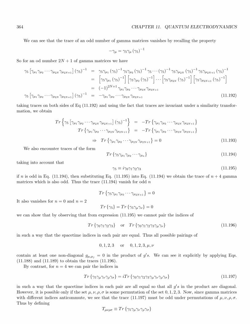
364 CHAPTER 11. QUANTUM ELECTRODYNAMICS
We can see that the trace of an odd number of gamma matrices vanishes by recalling the property
−γµ = γ5γµ (γ5)−1
So for an od number 2N + 1 of gamma matrices we have
γ5[γµ1γµ2 · · · γµ2Nγµ2N+1
](γ5)
−1 = γ5γµ1 (γ5)−1 γ5γµ2 (γ5)
−1 γ5 · · · (γ5)−1 γ5γµ2N (γ5)−1 γ5γµ2N+1
(γ5)−1
=[γ5γµ1 (γ5)
−1] [γ5γµ2 (γ5)
−1]· · ·[γ5γµ2N (γ5)
−1] [γ5γµ2N+1
(γ5)−1]
= (−1)2N+1 γµ1γµ2 · · · γµ2N γµ2N+1
γ5[γµ1γµ2 · · · γµ2Nγµ2N+1
](γ5)
−1 = −γµ1γµ2 · · · γµ2N γµ2N+1(11.192)
taking traces on both sides of Eq (11.192) and using the fact that traces are invariant under a similarity transfor-mation, we obtain
Trγ5[γµ1γµ2 · · · γµ2N γµ2N+1
](γ5)
−1
= −Trγµ1γµ2 · · · γµ2Nγµ2N+1
Trγµ1γµ2 · · · γµ2N γµ2N+1
= −Tr
γµ1γµ2 · · · γµ2Nγµ2N+1
⇒ Trγµ1γµ2 · · · γµ2N γµ2N+1
= 0 (11.193)
We also encounter traces of the form
Tr γ5γµ1γµ2 · · · γµn (11.194)
taking into account that
γ5 ≡ iγ0γ1γ2γ3 (11.195)
if n is odd in Eq. (11.194), then substituting Eq. (11.195) into Eq. (11.194) we obtain the trace of n+ 4 gammamatrices which is also odd. Thus the trace (11.194) vanish for odd n
Trγ5γµ1γµ2 · · · γµ2N+1
= 0
It also vanishes for n = 0 and n = 2
Tr γ5 = Tr γ5γµγν = 0
we can show that by observing that from expression (11.195) we cannot pair the indices of
Tr γ0γ1γ2γ3 or Tr γ0γ1γ2γ3γµγν (11.196)
in such a way that the spacetime indices in each pair are equal. Thus all possible pairings of
0, 1, 2, 3 or 0, 1, 2, 3, µ, ν
contain at least one non-diagonal gµiµj = 0 in the product of g′s. We can see it explicitly by applying Eqs.(11.188) and (11.189) to obtain the traces (11.196).
By contrast, for n = 4 we can pair the indices in
Tr γ5γµγνγργσ = iT r γ0γ1γ2γ3γµγνγργσ (11.197)
in such a way that the spacetime indices in each pair are all equal so that all g′s in the product are diagonal.However, it is possible only if the set µ, ν, ρ, σ is some permutation of the set 0, 1, 2, 3. Now, since gamma matriceswith different indices anticommute, we see that the trace (11.197) must be odd under permutations of µ, ν, ρ, σ.Thus by defining
Tµνρσ ≡ Tr γ5γµγνγργσ

11.11. SOME PROPERTIES OF “SLASH” MOMENTA 365
This is a totally antisymmetric structure of four indices in which each index can take four values. Therefore, thetrace (11.197) must be proportional to the totally antisymmetric tensor εµνρσ . We can determine the constant ofproportionality by setting µ, ν, ρ, σ → 0, 1, 2, 3 recalling that
ε0123 = −ε0123 = −1
then we obtainTr γ5γµγνγργσ = 4iεµνρσ (11.198)
using the same procedure to obtain Eq. (11.181) we can obtain the trace of products of γ5 with six, eight or moregamma matrices.
11.11 Some properties of “slash” momenta
From the Cliffrod algebra of the Dirac matrices we have
6 a 6 b = (aµγµ) (bνγ
ν) = aµbνγµγν = aµbν (2g
µν − γνγµ)
6 a 6 b = (2aµgµνbν − bνγ
νaµγµ)
6 a 6 b = 2a · b− 6 b 6 a (11.199)
in particular if the four-momenta a and b are orthogonal we obtain
6 a 6 b = − 6 b 6 a if a · b = 0 (11.200)
another interesting particular case appears from Eq. (11.199) by setting a = b
6 a2 = 2a2− 6 a2 ⇒ 6 a2 = a2 (11.201)
of course, in the scalars that appear in these identities we should multiply by a 4×4 unit matrix.We shall also encounter traces of products of slash momenta. We can calculate them by using the traces of
products of Dirac gamma matrices. For instance, using Eq. (11.193) we have
Tr 6 a1 6 a2 · · · 6 a2N+1 = Tr(aµ1γµ1) (a
µ2γµ2) · · ·(aµ2N+1γµ2N+1
)
= aµ1aµ2 · · · aµ2N+1Trγµ1γµ2 · · · γµ2N+1
Tr 6 a1 6 a2 · · · 6 a2N+1 = 0
Using Eq. (11.187) we have
Tr 6 a 6 b = Tr aµγµaνγν = aµaνTr γµγν = 4aµaνgµν
Tr 6 a 6 b = 4a · b
this result can also be obtained from Eq. (11.199) and the cyclic invariance of the trace
Tr 6 a 6 b = Tr 2 (a · b)14×4− 6 b 6 a = 2 (a · b)Tr 14×4 − Tr 6 b 6 aTr 6 a 6 b = 8 (a · b)− Tr 6 a 6 b ⇒ 2Tr 6 a 6 b = 8 (a · b)Tr 6 a 6 b = 4 (a · b)
now, from Eq. (11.188) we find
Tr 6 a 6 b 6 c 6 d = aµbνcρdσTr γµγνγργσ = 4aµbνcρdσ [gµνgρσ − gµρgνσ + gµσgνρ]
= 4 [(aµgµνbν) (cρgρσd
σ)− (aµgµρcρ) (bνgνσd
σ) + (aµgµσdσ) (bνgνρc
ρ)]
Tr 6 a 6 b 6 c 6 d = 4 [(a · b) (c · d)− (a · c) (b · d) + (a · d) (b · c)] (11.202)

Chapter 12
Path integral approach for bosons inquantum field theory
By applying the canonical quantization methods we were able to derive the Feynman rules for many theories.However, in the case of scalar fields with derivative couplings or the vector fields, we saw that the interactionHamiltonian contains a non-covariant term that is cancelled by a non-covariant term in the propagator1. Inquantum electrodynamics, the non-covariant term in the interacting Hamiltonian (the Coulomb energy) is notspatially local but it is local in time. Forgetting the cancellation process we can manage to use only the covariantterms to obtain the Feynman rules. However, this process of cancellation of non-covariant terms could be verydifficult to manage in non-abelian theories and in general relativity. Consequently, it is preferable a method thatuses the Lagrangian directly to derive the Feynman rules in a manifestly covariant form.
The path integral approach is a good alternative to work directly with a Lagrangian rather than a Hamiltonian.Indeed their are useful in non-abelian theories even when they exhibit spontaneous symmetry breaking, as is thecase of the standard model of weak and electromagnetic interactions. Moreover, path integral methods permit toaccount on the contributions to the S−matrix with an essential singularity at zero coupling constant that cannotbe discovered at any givne order in perturbation theory.
The reason to start with a canonical formalism lies in the fact that in such a formalism the S−matrix isclearly unitary. On the other hand, the path-integral formalism provides manifestly Lorentz invariance in thediagrammatic rules but the only way to show that the path-integral approach gives a unitary S−matrix is byreconstructing the canonical formalism in which unitarity is apparent. Hence, in the canonical formalism unitarityis apparent while Lorentz invariance is obscure and the opposite occurs with the path-integral formalism. Theadvantage of deriving the path-integral formalism from the canonical approach (as we shall do) is that we arecertain of having the same S−matrix in both formalisms. Consequently, we can guarantee for the S−matrix boththe Lorentz-invariance and unitarity.
A second reason to start with the canonical formalism has to do with the fact that for some importanttheories the simplest version of the path-integral approach (without starting with a canonical formalism) in whichpropagators and interaction vertices are taken directly from the Lagragian are wrong. This is the case with thenon-linear σ−model
L = −1
2gkmφ
(∂µφ
k)(∂µφm)
in which the Feynman ruels derived directly from the Lagrangian density would lead to a non-unitary and wrongS−matrix, that even depends on the way in which we define the scalar field. By deriving the path-integralapproach from a canonical formalism we are able to see the additional sorts of vertices required to correct thesimplest version of the Feynman path-integral formulation.
1The covariant term in the interaction Hamiltonian equals the negative of the interaction term in the Lagrangian.
366

12.1. THE GENERAL PATH-INTEGRAL FORMULA FOR BOSONIC OPERATORS 367
12.1 The general path-integral formula for bosonic operators
Let us assume a general quantum mechanical system with Hermitian bosonic operator “coordiantes” Qa andconjugate momenta Pb that satisfy canonical (bosonic) commutation (and NOT anticommutation) relations
[Qa, Pb] = iδab (12.1)
[Qa, Qb] = [Pa, Pb] = 0 (12.2)
we are assuming that any first class constraints are eliminated by choosing an apropriate gauge, and that theremaining second class constraints are solved by expressing the constrained variables in terms of the unconstrainedvariables Qa and Pa. Thus, we are dealing with independent canonical variables only.
The index a, is condensing continuous (position) indices as well as discrete ones (discrete Lorentz and speciesm indices)
Qa ≡ Qx,m ≡ Qm (x) (12.3)
Pa ≡ Px,m ≡ Pm (x) (12.4)
in the same way the kronecker delta in Eq. (12.1) means
δab ≡ δx,m ; y,n ≡ δ3 (x− y) δmn (12.5)
the operators defined so far are in the Schrodinger picture taken at a fixed time (e.g. t = 0).
Since the set of Q′a s commute, we can find a basis of simultaneous eigenstates |q〉 with eigenvalues qa
Qa |q〉 = qa |q〉 (12.6)
note that the lower case notation qa denotes eigenvalues instead of operators in the interaction picture. Such anotation is not misleading since we shall not use the interaction picture by now.
The eigenvectors of such a basis can be taken as orthonormal (in the extended sense)
⟨q′ |q〉 =
∏
a
δ(q′a − qa
)≡ δ
(q′ − q
)
with the corresponding completeness relation
1 =
∫ ∏
a
dqa |q〉 〈q|
in the same way we can find an orthonormal basis |p〉 of eigenvectors common to all P ′a s:
Pa |p〉 = pa |p〉 (12.7)⟨p′ |p〉 =
∏
a
δ(p′a − pa
)≡ δ
(p′ − p
)(12.8)
1 =
∫ ∏
a
dpa |p〉 〈p| (12.9)
Now from Eq. (12.1) it can be shown that Pb acts as a derivative operator −i∂/∂qb on wave functions on theq−basis. Then the wave function |p〉 in the basis |q〉 is given by
〈q |p〉 =∏
a
1√2π
exp (iqapa) (12.10)

368 CHAPTER 12. PATH INTEGRAL APPROACH FOR BOSONS IN QUANTUM FIELD THEORY
where the factor∏a
1√2π
is obtained from the normalization condition (12.8). On the other hand, Eq. (12.10) can
also be seen as the scalar product between the two complete orthonormal sets |q〉 and |p〉.In the Heisenberg picture, the canonical operators acquires time-dependence
Qa (t) ≡ exp (iHt) Qa exp (−iHt) (12.11)
Pa (t) ≡ exp (iHt) Pa exp (−iHt) (12.12)
where H is the total Hamiltonian. The canonical operators in the Heisenberg picture have eigenstates |q; t〉 and|p; t〉
Qa (t) |q; t〉 = qa |q; t〉Pa (t) |p; t〉 = pa |p; t〉
it is easy to obtain the basis |q; t〉 and |p; t〉 in terms of |q〉 and |p〉
Qa (t) |q; t〉 = qa |q; t〉 ⇒ exp (−iHt)Qa (t) exp (iHt) exp (−iHt) |q; t〉 = qa exp (−iHt) |q; t〉Qa [exp (−iHt) |q; t〉] = qa [exp (−iHt) |q; t〉]
and comparing with (12.6) we obtain
|q〉 = exp (−iHt) |q; t〉
and similarly for momenta eigenstates then we have
|q; t〉 = exp (iHt) |q〉 ; |p; t〉 = exp (iHt) |p〉 (12.13)
it worhts emphasizing that |q; t〉 is the eigenstate of Qa (t) with eigenvalue qa and it is NOT the time-evolutionof the state |q〉 for a time t. Owing to it, its time dependence is given by a factor exp (iHt) (i.e. the inverseof the time-evolution operator) instead that exp (−iHt). Once again, these states satisfy the completeness andorthonormality conditions
Qa (t) |q; t〉 = qa |q; t〉 ; Pa (t) |p; t〉 = pa |p; t〉⟨q′; t |q; t〉 =
∏
a
δ(q′a − qa
)≡ δ
(q′ − q
);⟨p′; t |p; t〉 ≡ δ
(p′ − p
)
∫ ∏
a
dqa |q; t〉 〈q; t| =
∫ ∏
a
dpa |p; t〉 〈p; t| = 1
as well as the product
〈q; t |p; t〉 =∏
a
1√2π
exp (iqapa) (12.14)
If after measuring at time t, our system becomes prepared at the state |q; t〉, the probability amplitude of findingit at the state |q′; t′〉 when we measure at time t′, is given by the scalar product
A ≡⟨q′; t′ |q; t〉 (12.15)
we shall focus on calculating this probability amplitude.

12.1. THE GENERAL PATH-INTEGRAL FORMULA FOR BOSONIC OPERATORS 369
12.1.1 Probability amplitude for infinitesimal time-intervals
The amplitude (12.15) is easier to calculate when the time interval involved is infinitesimal. From Eq. (12.13) wehave
⟨q′; τ + dτ |q; τ〉 =
⟨q′; τ
∣∣ exp (−iH dτ) |q; τ〉 (12.16)
Originally the Hamiltonian is expressed as a function H (Q,P ), but taking into account that the Hamiltoniancommutes with itself (and so with e±iHt), and that Eqs. (12.11) and (12.12) are similarity transformations, theHamiltonian can equally be written as the same function H (Q (t) , P (t))
H ≡ H (Q,P ) = eiHtH (Q,P ) e−iHt = H (Q (t) , P (t))
The Hamiltonian can be expressed in several forms through the commutation relations (12.1) and (12.2) by movingthe operators Q and P to obtain a given order. We shall settle it in a “standard form” or “normal order” with allQ′s to the left of all P ′s. As a matter of example, if a term of the form PaQbPc appears in the Hamiltonian, byusing Eq. (12.1), we have
PaQbPc = QbPaPc − iδabPc
by setting this normal order the Qa (t)′ s in the Hamiltonian of Eq. (12.16) could be replaced by the eigenvalue q′a of
Qa (t) associated with the bra. Notice that such a replacement is possible only because the operator exp [−iH dτ ]is linear in H for infinitesimal dτ . Now to deal with the P (t) operators (on the right) it is convenient to insertan identity involving their eigenvectors |p; τ〉⟨q′; τ + dτ |q; τ〉 =
∫ ∏
a
dpa⟨q′; τ
∣∣ exp [−iH (Q (τ) , P (τ)) dτ ] |p; τ〉 〈p; τ | q; τ〉
=
∫ ∏
a
dpa⟨q′; τ
∣∣ 1− iH (Q (τ) , P (τ)) dτ |p; τ〉 〈p; τ | q; τ〉
=
∫ ∏
a
dpa⟨q′; τ
∣∣ p; τ〉 〈p; τ | q; τ〉 − i
∫ ∏
a
dpa⟨q′; τ
∣∣ H (Q (τ) , P (τ)) dτ |p; τ〉 〈p; τ | q; τ〉
taking into account the order chosen for the Q,P operators in the Hamiltonian, we can replace H (Q (τ) , P (τ))by H (q′, p). In addition, by using the relation (12.14) we obtain
⟨q′; τ + dτ |q; τ〉 =
∫ ∏
a
dpa2π
exp
[−iH
(q′, p
)dτ + i
∑
a
(q′a − qa
)pa
](12.17)
with pa integrated over the interval (−∞,∞).
12.1.2 Probability amplitude for finite time intervals
We shall calculate 〈q′; t′ |q; t〉, for t < t′, by dividing the time interval from t to t′ into N + 1 intervals of equal“time length”
∆τ ≡ τk+1 − τk =(t′ − t)
N + 1; τ0 = t, τN+1 = t′ (12.18)
and insert a set of N identities associated with each time in the interior of the interval (so that we do not insertidentities associated with the edges τ0 = t and τN+1 = t′)
⟨q′; t′ |q; t〉 =
∫dq1 · · · dqN
⟨q′; t′
∣∣ qN ; τN 〉 〈qN ; τN | qN−1; τN−1〉 〈qN−1; τN−1| · · · |q1; τ1〉 〈q1; τ1 |q; t〉
(12.19)

370 CHAPTER 12. PATH INTEGRAL APPROACH FOR BOSONS IN QUANTUM FIELD THEORY
by definingq0 ≡ q ; qN+1 = q′
along with definitions (12.18) for τN+1 and τ0. We can rewrite (12.19) as
⟨q′; t′ |q; t〉 =
∫dq1 · · · dqN 〈qN+1; τN+1| qN ; τN 〉 〈qN ; τN | qN−1; τN−1〉 〈qN−1; τN−1| · · · |q1; τ1〉 〈q1; τ1 |q0; τ0〉
(12.20)
We have inner products of the type
〈qk+1; τk+1| qk; τk〉 ; k = 0, 1, 2, . . . , N
if N is large enough, the time intervals become small enough to apply the identity (12.17) valid for infinitesimaltime intervals
〈qk+1; τk+1 |qk; τk〉 ≈∫ ∏
a
dpa2π
exp
[−iH (qk+1, pk) ∆τ + i
∑
a
(qk+1,a − qk,a) pk,a
](12.21)
substituting (12.21) in (12.20) we find
⟨q′; t′ |q; t〉 ≈
∫ [ N∏
k=1
∏
a
dqk,a
][N∏
k=0
∏
a
dpk,a2π
]
× exp
i
N∑
k=0
[∑
a
(qk+1,a − qk,a) pk,a −H (qk+1, pk) ∆τ
](12.22)
where we have definedqa (τk) ≡ qk,a ; pa (τk) ≡ pk,a (12.23)
now we take the limit in which N → ∞ so that ∆τ ≡ dτ → 0. In that case the aproximation (12.22) becomesexact and we obtain
N ≡N∑
k=0
∑
a
(qk+1,a − qk,a) pk,a −H (qk+1, pk) dτ
=
N∑
k=0
∑
a
qa (τk) pa (τk)−H (q (τk) , p (τk))
dτ +O
((dτ)2
)
N →∫ t′
t
∑
a
qa (τ) pa (τ)−H (q (τ) , p (τ))
dτ (12.24)
additionally we can define integrals over the functions q (τ) and p (τ) as follows∫ ∏
τ,a
dqa (τ)∏
τ,b
dpb (τ)
2π· · · ≡ lim
dτ→0
∫ ∏
k,a
dqk,a∏
k,b
dpk,b2π
· · · (12.25)
therefore, Eq. (12.22) becomes a constrained path integral
⟨q′; t′ |q; t〉 =
∫qa(t)=qa
qa(t′)=q′a
∏
τ,a
dqa (τ)∏
τ,b
dpb (τ)
2π
× exp
i
∫ t′
tdτ
[∑
a
qa (τ) pa (τ)−H (q (τ) , p (τ))
](12.26)

12.1. THE GENERAL PATH-INTEGRAL FORMULA FOR BOSONIC OPERATORS 371
we call it a path integral because we are integrating over all paths that take q (τ) from q at τ = t to q′ at τ = t′,and also over all p (τ). We shall see that by writing the matrix elements as path integrals, we can calculate themeasily by expanding in powers of the coupling constants in H.
12.1.3 Calculation of matrix elements of operators through the path-integral formalism
In addition to amplitudes of probabilities we can obtain matrix elements between states 〈q′; t′| and |q; t〉 of time-ordered products of general operators of the form O (P (τ) , Q (τ)). In this case it is more convenient to definethese operators with all P ′s moved to the left of all Q′s. Thus, by inserting such an operator in Eq. (12.17) weobtain
M ≡⟨q′; τ + dτ
∣∣O (P (τ) , Q (τ)) |q; τ〉
=
∫ ∏
a
dpa⟨q′; τ
∣∣ exp [−iH (Q (τ) , P (τ)) dτ ] |p; τ〉 〈p; τ | O (P (τ) , Q (τ)) |q; τ〉
Owing to the order chosen for the operators Q,P in the Hamiltonian and in the operator O, we can make thereplacements
H (Q (τ) , P (τ)) → H(q′, p
)and O (P (τ) , Q (τ)) → O (p, q)
within the inner products. Then we can use the relation (12.14). The procedure is similar to the one that led toEq. (12.26)
⟨q′; τ + dτ
∣∣O (P (τ) , Q (τ)) |q; τ〉 =∫ ∏
a
dpa2π
exp
[−iH
(q′, p
)dτ + i
∑
a
(q′a − qa
)pa
]O (p, q) (12.27)
Now, to calculate the matrix element of a product of time ordered operators
OA1 (P (τA1) , Q (τA1)) OA2 (P (τA2) , Q (τA2)) · · · ; tA1 > tA2 > · · ·
we should insert these operators between the apropriate states in Eq. (12.19) [or Eq. (12.20)], and then utilizeEq. (12.27). For example, if tA1 lies between τk and τk+1, we should insert OA1 (P (τA1) , Q (τA1)) between〈qk+1; τk+1| and |qk; τk〉. We observe that in Eq. (12.19) each sucessive sum over states is at a later time, and it ispossible because of the assumption that tA1 > tA2 > · · · . With the same procedure as before, we find the generalpath-integral formula given by
MO ≡⟨q′; t′
∣∣OA1 (P (τA1) , Q (τA1)) OA2 (P (τA2) , Q (τA2)) · · · |q; t〉
=
∫qa(t)=qa
qa(t′)=q′a
∏
τ,a
dqa (τ)∏
τ,b
dpb (τ)
2πOA1 (p (τA1) , q (τA1)) OA2 (p (τA2) , q (τA2)) · · ·
× exp
i
∫ t′
tdτ
[∑
a
qa (τ) pa (τ)−H (q (τ) , p (τ))
](12.28)
in which we are assuming the time ordering given by
t′ > tA1 > tA2 > · · · > t
nevertheless, there is nothing on the right-hand side of Eq. (12.28) that refers to the order of time-arguments.Therefore, if we have a path integral of the form of the right-hand side of Eq. (12.28) but with tA1 , tA2 · · · inarbitrary order (except that they are all between t and t′ with t < t′), such a path integral is equal to a matrix

372 CHAPTER 12. PATH INTEGRAL APPROACH FOR BOSONS IN QUANTUM FIELD THEORY
element of the type of the left-hand side of Eq. (12.28), but with the operators ordered from left to right indecreasing time. Consequently for tA1 , tA2 , · · · in arbitrary order, the matrix element become
MTO ≡⟨q′; t′
∣∣T OA1 (P (τA1) , Q (τA1)) OA2 (P (τA2) , Q (τA2)) · · · |q; t〉
=
∫qa(t)=qa
qa(t′)=q′a
∏
τ,a
dqa (τ)∏
τ,b
dpb (τ)
2πOA1 (p (τA1) , q (τA1)) OA2 (p (τA2) , q (τA2)) · · ·
× exp
i
∫ t′
tdτ
[∑
a
qa (τ) pa (τ)−H (q (τ) , p (τ))
](12.29)
where as customary, T represents time-ordering of the operators.Note that the c−number functions qa (τ) and pa (τ) in Eq. (12.29) are unconstrained variables of integration
(each one is swept independently) and in particular they are not constrained to obey the classical equations ofmotion
qa (τ)−∂H (q (τ) , p (τ))
∂pa (τ)= 0 ; pa (τ) +
∂H (q (τ) , p (τ))
∂qa (τ)= 0 (12.30)
owing to it, the Hamiltonian H (q (τ) , p (τ)) in Eq. (12.29) is not constant in τ . Notwithstanding, in some sensepath integrals respect those equations of motion. Let us assume that one of the functions in Eq. (12.29) e.g.OA1 (P (τA1) , Q (τA1)), is the left hand side of either of Eqs. (12.30). It can be seen that for t < tA1 < t′ we have
[qa (tA1)−
∂H (q (tA1) , p (tA1))
∂pa (tA1)
]exp i I [q, p] = −i δ
δpa (tA1)exp i I [q, p]
[pa (tA1) +
∂H (q (tA1) , p (tA1))
∂qa (tA1)
]exp i I [q, p] = i
δ
δqa (tA1)exp i I [q, p]
with iI [q, p] being the argument of the exponential in Eq. (12.29)
I [q, p] ≡∫ t′
tdτ
∑
a
qa (τ) pa (τ)−H (q (τ) , p (τ))
whenever tA1 does not approach t nor t′, the integration over the variables qa (tA1) and pa (tA2) are not con-strained, and if they have well behavior in convergence, the integral of these variational derivatives must vanish.Consequently, the path integral given by (12.29) vanishes if OA1 (p, q) is taken to be the left.hand side of either ofthe equations of motion (12.30).
The rule above is valid only if the integration variables qa (tAi) , pa (tAi
) are independent of any other pair ofvariables qa (tAk
) , pa (tAk) that appears in any other function OAk
different from OAiin Eq. (12.29). Then, the
rule follows only if we forbid tAito approach tAk
with k 6= i, and also different from t and t′. If tAiapproaches
a given tAk, the path integral will contain a non-zero term proportional to δ (tAi
− tAk) or its derivatives. These
are the same delta function that we encounter in the operator formalism coming from time derivatives of stepfunctions that are implicit in the definition of time-ordered products.
In order to evaluate the path integrals (12.26) or (12.29) it suffices to know the classical Hamiltonian as ac−number function H (q, p). In formulating a path integral approach a natural question is how to choose theHamiltonian after the quantization H (Q,P ). Certainly, there are several Hamiltonians that differs only in theorder in which the Q′s and P ′s are put after quantization. According to our developments the apropriate choiceseems to be the one with all Q′s on the left and all P ′s on the right. However, such a choice depends on theinterpretation given to the measure ∏
dqa (τ)∏
dpb (τ)
that appears in the path integrals (12.26) or (12.29). The prescription of all Q′s on the left and all P ′s on theright is correct only if the measured is interpreted according with Eqs. (12.23), (12.24) and (12.25). With other

12.2. PATH FORMALISM FOR THE S−MATRIX 373
measures we would have other prescription for the ordering of the operators. Nevertheless, different prescriptionsfor ordering the operators in the Hamiltonian lead to different choices of the constants that appear as coefficients inthe various terms of the Hamiltonian. Since such coefficients are considered arbitrary parameters (to be adjustedby phenomenology) any prescription is physically equivalent to any other.
The path integral form (12.29) is not adequate for numerical calculations or to prove theorems. In that case itis more advantageous to use a path integral method in which we calculate amplitudes in the Euclidean space witht substituted by −ix4, so that the exponential in Eq. (12.29) becomes a negative real quantity. In the Minkowskispace, we have oscillating paths generating rapid oscillations of the integrand from one path to another. By usingthe Euclidean space, the oscillating paths are exponentially supressed. Indeed we could start directly from apath integral formulation in the Euclidean space or pass from one formulation to the other. By now, we use theMinkowski space since our main goal is to calculate Feynman amplitudes with a perturbation approach.
12.2 Path formalism for the S−matrix
The results so far are valid in the framework of ordinary quantum mechanics. A more suitbale notation forquantum field theory is obtained by setting the index a to run over points x in space and over a spin and speciesindex m so that we replace
Qa (t) → Qm (x, t) ; Pa (t) → Pm (x, t)
further, we also rewrite
H (q (t) , p (t)) → H [q (t) , p (t)] ; O (p (t) , q (t)) → H [p (t) , q (t)]
to emphasize that the Hamiltonian and operators are functionals of qm (x, t) and pm (x, t) at a given time t. Fromthese facts, we rewrite Eq. (;;;) as
MTO ≡⟨q′; t′
∣∣T OA1 [P (tA1) , Q (tA1)] OA2 [P (tA2) , Q (tA2)] · · · |q; t〉
=
∫qm(x,t)=qm(x)
qm(x,t′)=q′m(x)
∏
τ,x,m
dqm (x, τ)∏
τ,x,m
dpm (x, τ)
2πOA1 [p (tA1) , q (tA1)] OA2 [p (tA2) , q (tA2)] · · ·
× exp
i
∫ t′
tdτ
[∫d3x
∑
m
qm (x, τ) pm (x, t)−H [q (τ) , p (τ)]
](12.31)

Bibliography
[1] Steven Weinberg, The Quantum Theory of Fields. Vol. I: Foundations. Cambridge University Press(1995).
[2] Steven Weinberg, The Quantum Theory of Fields.Vol. II: Modern Applications. Cambridge UniversityPress (1996).
[3] Steven Weinberg, The Quantum Theory of Fields. Vol. III: Supersymmetry. Cambridge UniversityPress (2000).
[4] Lewis H. Ryder, Quantum Field Theory (Second Ed.). Cambridge University Press (1996).
[5] Michio Kaku, Quantum Field Theory, a modern introduction. Oxford University Press (1993).
[6] John Collins, Renormalization. Cambridge Monographs on Mathematical Physics. Cambridge UniversityPress (1984).
[7] Claude Itzykson, Jean-Bernard Zuber,Quantum Field Theory. McGraw-Hill International Editions, PhysicsSeries (1980).
374


