192
Quantum memory: design and applications Fernando Pastawski M¨ unchen 2012
| Date post: | 04-Apr-2018 |
| Category: |
Documents |
| Upload: | trinhkhuong |
| View: | 220 times |
| Download: | 3 times |

Quantum memory:
design and applications
Fernando Pastawski
Munchen 2012

Quantum memory:
design and applications
Fernando Pastawski
Dissertation
an der
Ludwig-Maximilians-Universitat
Munchen
vorgelegt von
Fernando Pastawski
aus Cordoba, Argentinien
Munchen, den 4.6.2012
Tag der mundlichen Prufung: 26.7.2012
Erstgutachter: Prof. J. I. Cirac
Zweitgutachter: Prof. H. Weinfurter
Weitere Prufungskommissionsmitglieder: Prof. J. von Delft , Prof. T. Liedl

Abstract
This thesis is devoted to the study of coherent storage of quantum information as well as
its potential applications. Quantum memories are crucial to harnessing the potential of
quantum physics for information processing tasks. They are required for almost all quantum
computation proposals. However, despite the large arsenal of theoretical techniques and
proposals dedicated to their implementation, the realization of long-lived quantum memories
remains an elusive task.
Encoding information in quantum states associated to many-body topological phases of
matter and protecting them by means of a static Hamiltonian is one of the leading proposals
to achieve quantum memories. While many genuine and well publicized virtues have been
demonstrated for this approach, equally real limitations were widely disregarded. In the first
two projects of this thesis, we study limitations of passive Hamiltonian protection of quantum
information under two different noise models.
Chapter 2 deals with arbitrary passive Hamiltonian protection for a many body system
under the effect of local depolarizing noise. It is shown that for both constant and time de-
pendent Hamiltonians, the optimal enhancement over the natural single-particle memory time
is logarithmic in the number of particles composing the system. The main argument involves
a monotonic increase of entropy against which a Hamiltonian can provide little protection.
Chapter 3 considers the recoverability of quantum information when it is encoded in a
many-body state and evolved under a Hamiltonian composed of known geometrically local
interactions and a weak yet unknown Hamiltonian perturbation. We obtain some
generic criteria which must be fulfilled by the encoding of information. For specific proposals
of protecting Hamiltonian and encodings such as Kitaev’s toric code and a subsystem code
proposed by Bacon, we additionally provide example perturbations capable of destroying the
memory which imply upper bounds for the provable memory times.
vi Abstract
Chapter 4 proposes engineered dissipation as a natural solution for continuously ex-
tracting the entropy introduced by noise and keeping the accumulation of errors under control.
Persuasive evidence is provided supporting that engineered dissipation is capable of preserv-
ing quantum degrees of freedom from all previously considered noise models. Furthermore, it
is argued that it provides additional flexibility over Hamiltonian thermalization models and
constitutes a promising approach to quantum memories.
Chapter 5 introduces a particular experimental realization of coherent storage, shifting
the focus in many regards with respect to previous chapters. First of all, the system is very
concrete, a room-temperature nitrogen-vacancy centre in diamond, which is subject
to actual experimental control and noise restrictions which must be adequately modelled.
Second, the relevant degrees of freedom reduce to a single electronic spin and a carbon 13 spin
used to store a qubit. Finally, the approach taken to battle decoherence consists of inducing
motional narrowing and applying dynamical decoupling pulse sequences, and is tailored to
address the systems dominant noise sources.
Chapter 6 analyses unforgeable tokens as a potential application of these room-temperature
qubit memories. Quantum information protocols based on Wiesner’s quantum money scheme
are proposed and analysed. We provide the first rigorous proof that such unentangled tokens
may be resistant to counterfeiting attempts while tolerating a certain amount of noise.
In summary, this thesis provides contributions to quantum memories in four different as-
pects. Two projects were dedicated to understanding and exposing the limitations of existing
proposals. This is followed by a constructive proposal of a new counter-intuitive theoretical
model for quantum memories. An applied experimental project achieves record coherent stor-
age times in room-temperature solids. Finally, we provide rigorous analysis for a quantum
information application of quantum memories. This completes a broad picture of quantum
memories which integrates different perspectives, from theoretical critique and constructive
proposal, to technological application going through a down-to-earth experimental implemen-
tation.
Zusammenfassung
Diese Arbeit widmet sich der koharenten Speicherung von Quanteninformation, sowie ihren
potenziellen Anwendungen. Quantenspeicher sind wesentlich, wenn es darum geht das Po-
tential der Quantenmechanik fur Aufgaben der Informationsverarbeitung zu nutzen. Sie sind
Voraussetzung in nahezu allen Vorschlagen zur Realisierung von Quantencomputern. Trotz
der Fulle an theoretischen Methoden und Vorschlagen zu ihrer experimentellen Implemen-
tierung, steht die Realisierung eines langlebigen Quantenspeichers bis heute aus.
Einer der vielversprechendsten Ansatze zur Implementierung von Quantenspeichern ist
es, Information in Quantenzustanden, die zu topologischen Phasen in Vielteilchensystemen
gehoren und durch einen statischen Hamiltonoperator geschutzt werden, zu codieren. Wahrend
auf der einen Seite die Vorzuge dieses Ansatzes viel Beachtung gefunden haben und in zahlre-
ichen Arbeiten diskutiert wurden, hat man auf der anderen Seite viele ebenso wichtige
Einschrankungen bislang weitgehend ignoriert. In den ersten beiden Projekten dieser Ar-
beit untersuchen wir Schwierigkeiten, die bei dem Versuch Quanteninformation passiv durch
Hamiltonoperatoren zu schutzen, auftreten. Hierbei konzentrieren wir uns auf zwei unter-
schiedliche Modelle zur Beschreibung der ausseren Storeinflusse.
Kapitel zwei befasst sich mit den Moglichkeiten ein System, das lokalem depolarisieren-
den Rauschen ausgesetzt ist, durch beliebige Hamiltonoperatoren passiv zu schutzen. Wir
zeigen, dass sich die optimale Erhohung der Speicherzeit im Vergleich zu Einteilchenspeich-
ern sowohl fur konstante als auch zeitabhangige Hamiltonoperatoren logarithmisch zu der
Teilchenzahl, aus denen das System besteht, verhalt. Die Hauptursache fur dieses Verhalten
liegt in dem monotonen Anstieg der Entropie.
In Kapitel drei betrachten wir Systeme die einer Zeitentwicklung durch Hamiltonop-
eratoren, die durch bekannte lokale Wechselwirkungen und eine beliebige hamiltonsche
Storung beschrieben werden, ausgesetzt sind. Wir leiten allgemeine Kriterien, die von der

viii Zusammenfassung
codierten Information erfullt werden mussen, her. Fur spezifische Hamiltonoperatoren und
Codierungen, wie Kitaevs torischen Code und Bacons 3D Kompas Code, beschreiben wir
Beispiele von Storungen, die dazu in der Lage sind den Speicher zu zerstoren. Dies impliziert
eine obere Beschrankung fur Speicherzeiten, die bewiesen werden konnen.
In Kapitel vier stellen wir ein Konzept vor, mit welchem Entropie, die dem System durch
Rauschen zugefuhrt wurde, durch manipulierbare Dissipation kontinuierlich extrahiert wer-
den kann. Gleichzeitig wird dabei die Akkumulation von Fehlern unter Kontrolle gehalten.
Wir zeigen, dass manipulierbare Dissipation die Quanteneigenschaften von all den von uns
betrachteten Modellen fur Rauschen erhalt.
In Kapitel funf betrachten wir eine konkrete Realisierung von koharentem Speichern.
Hier geht es um eine konkrete physikalische Anwendung in einem NV-Zentrum, in der ex-
perimentelle Kontrollmoglichkeiten und realistische Bedingungen fur das Rauschen in Be-
tracht gezogen und adaquat modelliert werden mussen. Der Bewegungsfreiheitsgrad ist in
diesem System auf nur einen Elektronenspin und einen Kohlenstoff-13 Kernspin beschrankt.
Das Konzept, das wir hier zur Bekampfung von Dekoharenz vorschlagen, besteht aus Bewe-
gungsmittelung und dynamischen Entkopplungs-Pulssequenzen und ist auf das System und
seine vornehmlichen Quellen fur Rauschen optimiert.
Solch ein Quantenspeicher fur Quantenbits in NV-Zentren, der bei Raumtemperatur funk-
tionsfahig ist, stellt unsere Motivation fur Kapitel sechs dar. Dort stellen wir Konzepte vor,
welche die Realisierung falschungssicherer Sicherheitslosungen mit derartigen Quantenbits er-
lauben. Basierend auf Wiesners Quantengeld-Schema entwickeln wir neue Quanteninformations-
Protokolle. Wir stellen hier den ersten rigorosen Beweis vor, dass derartige unverschrankte
Sicherheitslosungen gegen Falschungsversuche sicher waren und außerdem eine bestimmte
Menge an Rauschen tolerieren konnten.
Zusammenfassend liefert diese Doktorarbeit einen Beitrag zu Quantenspeichern aus vier
verschiedenen Perspektiven. Zwei Projekte sind dem Verstandnis und den Limitierungen von
bestehenden Konzepten gewidmet. Dann stellen wir ein neuartiges, kontraintuitives, theo-
retisches Konzept zur Realisierung eines Quantenspeichers vor. In Kollaboration mit einer
experimentellen Arbeit ist der Rekord von koharenten Speicherzeiten bei Raumtemperatur
gebrochen worden. Außerdem stellen wir eine rigorose Beschreibung von Quanteninforma-
tionsanwendungen fur Quantenspeicher vor.

Contents
Abstract v
Zusammenfassung vii
Publications xiii
1 Introduction 1
2 Hamiltonian memory model under depolarizing noise 9
2.1 Introduction . . . . . . . . . . . . . . . . . . . . . . . . . . . . . . . . . . . . . 9
2.2 Protection limitations . . . . . . . . . . . . . . . . . . . . . . . . . . . . . . . 11
2.3 Time dependent protection . . . . . . . . . . . . . . . . . . . . . . . . . . . . 12
2.4 Time-independent protection . . . . . . . . . . . . . . . . . . . . . . . . . . . 13
2.4.1 Clock dependent Hamiltonian . . . . . . . . . . . . . . . . . . . . . . . 16
2.4.2 Error analysis . . . . . . . . . . . . . . . . . . . . . . . . . . . . . . . . 17
2.5 Conclusions . . . . . . . . . . . . . . . . . . . . . . . . . . . . . . . . . . . . . 18
3 Hamiltonian memory model under Hamiltonian perturbations 21
3.1 Introduction . . . . . . . . . . . . . . . . . . . . . . . . . . . . . . . . . . . . 21
3.1.1 Noise model motivation . . . . . . . . . . . . . . . . . . . . . . . . . . 25
3.1.2 Outline of results . . . . . . . . . . . . . . . . . . . . . . . . . . . . . . 27
3.2 Subsystems instead of subspaces . . . . . . . . . . . . . . . . . . . . . . . . . 29
3.2.1 Eigenstate susceptibility to perturbations . . . . . . . . . . . . . . . . 30
3.2.2 State evolution in coupled Hamiltonians . . . . . . . . . . . . . . . . 31
3.2.3 Discussion . . . . . . . . . . . . . . . . . . . . . . . . . . . . . . . . . . 34
x CONTENTS
3.3 Error threshold required . . . . . . . . . . . . . . . . . . . . . . . . . . . . . 35
3.4 Limitations of the 2D toric code . . . . . . . . . . . . . . . . . . . . . . . . . 38
3.4.1 Probabilistic introduction of distant anyons . . . . . . . . . . . . . . . 38
3.4.2 Simple error loops in O(N) time . . . . . . . . . . . . . . . . . . . . . 42
3.4.3 Localization in 2D stabilizer codes . . . . . . . . . . . . . . . . . . . . 43
3.4.4 Logical errors in O(logN) time . . . . . . . . . . . . . . . . . . . . . . 44
3.4.5 Discussion . . . . . . . . . . . . . . . . . . . . . . . . . . . . . . . . . . 47
3.5 Limitations of the 2D Ising model . . . . . . . . . . . . . . . . . . . . . . . . 49
3.5.1 Hamiltonian perturbation proposal . . . . . . . . . . . . . . . . . . . . 50
3.5.2 Discussion . . . . . . . . . . . . . . . . . . . . . . . . . . . . . . . . . . 51
3.6 Aggressive noise models . . . . . . . . . . . . . . . . . . . . . . . . . . . . . . 52
3.6.1 Time-varying Perturbations . . . . . . . . . . . . . . . . . . . . . . . . 52
3.6.2 Stabilizer Hamiltonians and energetic environment . . . . . . . . . . . 54
3.6.3 Non-stabilizer Hamiltonians . . . . . . . . . . . . . . . . . . . . . . . . 56
3.7 Further applications . . . . . . . . . . . . . . . . . . . . . . . . . . . . . . . . 58
3.8 Conclusions . . . . . . . . . . . . . . . . . . . . . . . . . . . . . . . . . . . . . 59
3.A State evolution in perturbed gapped Hamiltonians . . . . . . . . . . . . . . . 61
3.B The toric code . . . . . . . . . . . . . . . . . . . . . . . . . . . . . . . . . . . 63
3.C Full Depolarization of the Toric Code’s Protected Subspace . . . . . . . . . . 66
4 Quantum memories based on engineered dissipation 71
4.1 Introduction . . . . . . . . . . . . . . . . . . . . . . . . . . . . . . . . . . . . . 71
4.2 Statement of the problem . . . . . . . . . . . . . . . . . . . . . . . . . . . . . 74
4.3 Straightforward QECC encoding . . . . . . . . . . . . . . . . . . . . . . . . . 75
4.3.1 Single Jump Operator . . . . . . . . . . . . . . . . . . . . . . . . . . . 76
4.3.2 Concatenated QECC Dissipation . . . . . . . . . . . . . . . . . . . . . 77
4.4 Local dissipative protection in 4D . . . . . . . . . . . . . . . . . . . . . . . . 78
4.4.1 Numerical simulations . . . . . . . . . . . . . . . . . . . . . . . . . . . 79
4.5 Accessible toy model . . . . . . . . . . . . . . . . . . . . . . . . . . . . . . . 80
4.6 Dissipative gadgets . . . . . . . . . . . . . . . . . . . . . . . . . . . . . . . . 81
4.7 Conclusions and perspectives . . . . . . . . . . . . . . . . . . . . . . . . . . . 83
4.A Adiabatic elimination of ancilla . . . . . . . . . . . . . . . . . . . . . . . . . . 84

CONTENTS xi
4.B 4D Toric code . . . . . . . . . . . . . . . . . . . . . . . . . . . . . . . . . . . 86
4.B.1 The 4D Toric code as a stabilizer code . . . . . . . . . . . . . . . . . . 86
4.B.2 Logical degrees of freedom . . . . . . . . . . . . . . . . . . . . . . . . . 87
4.B.3 4D PBC lattice notation . . . . . . . . . . . . . . . . . . . . . . . . . . 87
4.B.4 4D Quantum Toom’s rule . . . . . . . . . . . . . . . . . . . . . . . . . 88
4.B.5 Full recovery and error corrected operators . . . . . . . . . . . . . . . 89
4.B.6 Master equation . . . . . . . . . . . . . . . . . . . . . . . . . . . . . . 89
4.B.7 Numerical considerations . . . . . . . . . . . . . . . . . . . . . . . . . 91
4.B.8 Definition of efficient recovery R . . . . . . . . . . . . . . . . . . . . . 91
4.C Concatenated-code dissipation . . . . . . . . . . . . . . . . . . . . . . . . . . 91
4.C.1 Bounding error probabilities . . . . . . . . . . . . . . . . . . . . . . . . 96
4.D Proof of independence for the Enabled property . . . . . . . . . . . . . . . . . 98
5 Record qubit storage time using NV-center proximal 13C 101
5.1 Introduction . . . . . . . . . . . . . . . . . . . . . . . . . . . . . . . . . . . . . 101
5.1.1 Outline . . . . . . . . . . . . . . . . . . . . . . . . . . . . . . . . . . . 102
5.2 An introduction to NV centers . . . . . . . . . . . . . . . . . . . . . . . . . . 102
5.2.1 Electronic energy levels . . . . . . . . . . . . . . . . . . . . . . . . . . 104
5.2.2 Electronic spin sublevels . . . . . . . . . . . . . . . . . . . . . . . . . . 105
5.2.3 Nuclear spin environment . . . . . . . . . . . . . . . . . . . . . . . . . 105
5.3 Qubit initialization and readout . . . . . . . . . . . . . . . . . . . . . . . . . . 107
5.3.1 Electronic spin initialization and readout . . . . . . . . . . . . . . . . 108
5.3.2 CnNOTe . . . . . . . . . . . . . . . . . . . . . . . . . . . . . . . . . . 108
5.3.3 Nuclear spin gates and preparation of arbitrary states . . . . . . . . . 110
5.3.4 Repetitive readout and initialization . . . . . . . . . . . . . . . . . . . 110
5.4 Nuclear spin coherence and depolarization . . . . . . . . . . . . . . . . . . . . 113
5.4.1 Spin fluctuator model and motional narrowing . . . . . . . . . . . . . 113
5.4.2 Decoupling of homo-nuclear dipole-dipole interactions . . . . . . . . . 117
5.5 Conclusions and perspective . . . . . . . . . . . . . . . . . . . . . . . . . . . . 119
6 Unforgeable noise-tolerant quantum tokens 123
6.1 Introduction . . . . . . . . . . . . . . . . . . . . . . . . . . . . . . . . . . . . . 124
xii Inhaltsverzeichnis
6.2 Qticket . . . . . . . . . . . . . . . . . . . . . . . . . . . . . . . . . . . . . . . . 124
6.3 Cv-qticket . . . . . . . . . . . . . . . . . . . . . . . . . . . . . . . . . . . . . . 125
6.4 Applications . . . . . . . . . . . . . . . . . . . . . . . . . . . . . . . . . . . . . 128
6.5 Discussion . . . . . . . . . . . . . . . . . . . . . . . . . . . . . . . . . . . . . . 129
6.A Notation and external results . . . . . . . . . . . . . . . . . . . . . . . . . . . 131
6.B Qtickets . . . . . . . . . . . . . . . . . . . . . . . . . . . . . . . . . . . . . . . 133
6.B.1 Definition of qtickets . . . . . . . . . . . . . . . . . . . . . . . . . . . . 133
6.B.2 Soundness . . . . . . . . . . . . . . . . . . . . . . . . . . . . . . . . . . 134
6.B.3 Security . . . . . . . . . . . . . . . . . . . . . . . . . . . . . . . . . . . 135
6.B.4 Tightness . . . . . . . . . . . . . . . . . . . . . . . . . . . . . . . . . . 141
6.B.5 Extension: Issuing multiple identical qtickets . . . . . . . . . . . . . . 142
6.C CV-Qtickets . . . . . . . . . . . . . . . . . . . . . . . . . . . . . . . . . . . . . 143
6.C.1 CV-Qticket definition . . . . . . . . . . . . . . . . . . . . . . . . . . . 143
6.C.2 Soundness . . . . . . . . . . . . . . . . . . . . . . . . . . . . . . . . . . 143
6.C.3 Security . . . . . . . . . . . . . . . . . . . . . . . . . . . . . . . . . . . 144
6.C.4 Quantum retrieval games . . . . . . . . . . . . . . . . . . . . . . . . . 145
6.C.5 CV-Qticket qubit pair building block . . . . . . . . . . . . . . . . . . . 151
6.C.6 CV-Qticket retrieval games . . . . . . . . . . . . . . . . . . . . . . . . 152
6.C.7 Combinatorial bound on choosing and learning . . . . . . . . . . . . . 153
6.D Applications . . . . . . . . . . . . . . . . . . . . . . . . . . . . . . . . . . . . . 155
6.D.1 Enforcing single usage with a single verifier . . . . . . . . . . . . . . 155
6.D.2 Multiple non communicating verifiers . . . . . . . . . . . . . . . . . . 155
6.D.3 Reduced availability under sporadic verification . . . . . . . . . . . . . 156
6.D.4 The quantum credit card . . . . . . . . . . . . . . . . . . . . . . . . . 157
6.D.5 Excluding eavesdropers . . . . . . . . . . . . . . . . . . . . . . . . . 157
Acknowledgements 177

PhD Publications
This thesis is based on the following publications, which resulted from research conducted
during the author’s PhD. Some copyrighted material from these articles is reproduced with
permission of APS, AAAS, PNAS and Rinton editorial.
1. How Long Can a Quantum Memory Withstand Depolarizing Noise?
Fernando Pastawski, Alastair Kay, Norbert Schuch, and J. Ignacio Cirac
Phys. Rev. Lett. 103, 080501 (2009). (See chapter 2) as well as the original published
article appended to this thesis with permission of APS.
2. Limitations of Passive Protection of Quantum Information
Fernando Pastawski, Alastair Kay, Norbert Schuch, and J. Ignacio Cirac
Quant. Inf. and Comp. 10, (7&8) 0580-0618 (2010). (See chapter 3)
3. Quantum memories based on engineered dissipation
Fernando Pastawski, Lucas Clemente, and J. Ignacio Cirac
Phys. Rev. A 83, 012304 (2011). (See chapter 4)
4. Room-Temperature Quantum Bit Memory Exceeding One Second
Peter C. Maurer, Georg Kucsko, Christian Latta, Liang Jiang, Norman Y. Yao, S.
Bennett, Fernando Pastawski, D. Hunger, N. Chisholm, M. Markham, D. Twitchen, D.
J. Ignacio Cirac, and Mikail D. Lukin
Science 336 1283-1286 (2012). (See chapter 5) as well as the original published article
appended to this thesis with permission from AAAS.
5. Unforgeable Noise-Tolerant Quantum Tokens
Fernando Pastawski, Norman Y. Yao, Liang Jiang, Mikhail D. Lukin, and J. Ignacio
Cirac arXiv:1112.5456 (2011). (See chapter 6)

xiv Publications
Chapter 1
Introduction
Quantum mechanics is the well established physical theory describing the world below the
Planck scale. With the advent of integrated circuits and Moore’s law [92] predicting a doubling
in their transistor density every two years, it soon became clear that it would eventually
become necessary to seriously take quantum effects into account. In this context, some ideas
of quantum computing and quantum information unavoidably began to emerge in the 1970’
and early 1980’ in the minds of physicists and computer scientists such as Charles H. Bennett,
Paul A. Benioff, David Deutsch and Richard P. Feynman [17, 15, 40, 33]. It was time to move
on from the models of billiard ball computing and embrace the era of quantum information.
While it became clear early on [33] that a quantum computer would be at least as pow-
erful as a classical one, expected advantages of a quantum computer were apparently limited
to simulating quantum-mechanical systems [40] in addition to solving a few relatively con-
trived mathematical problems. There was also no pressing urge from the microelectronics
industry to better understand the workings of quantum information. This all changed with
the break-through result of Peter Shor [112], who in 1994 proposed an algorithm by which
a quantum computer could factor large numbers in a time exponentially faster than most
practical classical algorithms. If implemented, Shors algorithm could be used to crack main-
stream cryptographic codes such as RSA [107] for which the difficulty of factoring is essential.
Since then, quantum computation has received a huge amount of attention, not only from
the scientific community, but from the whole world.
Ironically, in their seminal work of 1984, Charles Bennett and Gilles Brassard [16] had
already proposed a quantum key distribution scheme, which could potentially substitute RSA

2 1. Introduction
allowing for cryptographically secure private communication even in a world with quantum
computers. However, contrary to popular belief, this was not the first cryptographic protocol
relying on the quantum nature of information. Stephen Wiesner[129], had been ahead of
his time in proposing the use of bank notes which were impossible to duplicate due to the
quantum character of the state defining them, a topic which we will get back to in the last
chapter of this thesis.
As illustrated, quantum computing and quantum information are both of technological
and fundamental appeal. This brings us to the topic of this thesis, quantum memories, which
are expected to play a central role in the implementation of quantum information technologies.
They are required to perform entanglement swapping and are thus crucial for long-distance
quantum key distribution. They are necessary in almost all models of quantum computation,
where it is ubiquitous to have data wait. Finally, the quality of a quantum memory constitutes
a benchmark for the degree of coherent quantum control achievable within a system and may
be used to compare different technologies.
This thesis is devoted to the understanding and design of quantum memories and their
applications. We present the five projects in the subsequent chapters with these general goals
in mind. The first two (chapters 2 and 3) explore existing proposals for many-body quan-
tum memories exposing their limitations and understanding their virtues. The following two
(chapters 4 and 5) propose implementations of quantum memories, first paying attention to
scaling in an abstract many-body context and later concentrating on a concrete experimental
quantum optics setting, namely Nitrogen-vacancy centers. Inspired by record coherence times,
in the chapter 6, we propose an application consisting of tokens impossible to counterfeit.
The main contributions of this thesis are to the field of many-body quantum memories
(chapters 2 , 3 and 4). In order to better understand these contributions, it is convenient to set
the context in terms of pre-existing developments such as fault-tolerant quantum computation
[47] and topological quantum memory [73, 32, 74].
The theory of fault-tolerant quantum computation [47] proves that it is possible to sim-
ulate an ideal circuit model quantum computer using only imperfect (yet sufficiently good)
single and two qubit gates, initialization of ancillary qubits and measurements. Quantum
memories may be seen as representing the most trivial computation, the identity. In particu-
lar, one should be able to compute the identity function within universal models of quantum
3
computation such as the fault tolerant circuit model. In practice however, the experimental
requirements imposed by fault tolerant quantum computation have up to now proven pro-
hibitively difficult to achieve. This has motivated ongoing research to find alternative routes
to both quantum computing and quantum memory.
Topological quantum computing and quantum memory, a revolutionary idea introduced
by Kitaev in 1997 [73, 32, 74], promises to attain fault-tolerance by means of an alternate
route, more akin to physics than to circuit engineering. At the core of this approach is the
independence of an anyonic quasi-particle picture from specific microscopic details of the
defining Hamiltonian. During the time of this thesis and the period preceding it many of the
claims pertaining to these proposals have been rigorously proven, and some of the folklore
that has arisen from it has been dissipated. The contributions of chapter 2 and 3 have been
partly responsible for this.
The toric code [74] is the most simple and hence the most widely popularized representative
for the topological approach to fault tolerance. It is associated to two related, yet distinct,
concepts both involving physical qubits placed on the edges of a 2d lattice on a torus. First,
the toric code refers to a stabilizer quantum error correcting code accommodating two
logical qubits. As such, it enjoys desirable properties such as
• Geometrically local check operators: Only quantum measurements involving groups
of four nearest neighbour qubits are needed in order to diagnose physical errors.
• Large code distance: The minimal number of single qubits that must be acted upon
in order to go from one logical state to an orthogonal one is proportional to the perimeter
of the torus. 1
• High error threshold: The code is capable of correcting random flip and phase errors
on up to ≈11% of the qubits in the limit of large torus.
Second, the toric-code Hamiltonian is obtained from interpreting the Hermitian stabilizer
operators as local Hamiltonian terms acting on groups of two-level systems. The resulting
Hamiltonian enjoys the following properties:
• Geometrically local interaction: Geometrically local terms in the Hamiltonian can
be associated to geometry local effective interactions.
1By perimeter, we mean the minimal number of edges to non-trivially wind around the torus.
4 1. Introduction
• Degenerate ground state: Information can be thought of as being accommodated in
a 4-fold degenerate ground space.2
• Robust degeneracy: For a weak geometrically local yet extensive perturbation, the
degeneracy of the ground space is approximately preserved.
• Energy gap: An energy gap suggests that excitations out of the ground space could
be thermally suppressed.
These two related notions of toric code have regretfully led to some confusion among part
of the quantum information community. The wide-spread belief that implementing a toric
code Hamiltonian would guarantee a quantum memory to be protected against any form
of local noise is a paragon example of such misconception. Results provided in this thesis
have been crucial in rigorously elucidating limitations of Hamiltonian protection models and
proposing alternatives to overcome them.
In particular, chapter 2 provides a definite proof that no Hamiltonian may by itself provide
significant protection against depolarizing noise. We consider a system which is subject
to both a unitary evolution generated by a Hamiltonian and the dissipative effect of local
depolarizing noise over the constituent particles. The motivation behind choosing a local
depolarizing noise model can be traced to infrequent yet highly energetic interactions capable
of randomizing the state of single components. For this noise model the approach towards a
maximally mixed steady state may not be postponed by a Hamiltonian. Entropy accumulates
at an unavoidable rate, and all that can be achieved by a Hamiltonian is to transfer it into
irrelevant degrees of freedom. We show that the optimal protection afforded by a constant
Hamiltonian only marginally increases the lifetime of quantum information from constant to
logarithmic in the number of system constituents.
Along similar lines, chapter 3 studies the degree of protection that may be afforded by
a protecting Hamiltonian against Hamiltonian perturbations and perturbative coupling to
an environment. Contrasting with the previous chapter, possible evolutions are unitary yet
our ignorance of the specific perturbation applied and/or entanglement with the environment
lead to effective loss of information. We show that an encoding through an error correcting
2The degeneracy of the ground space only depends on the genus of the surface represented by the lattice,
hence the name topological.
5
code with a finite error threshold is a necessary condition for information to withstand such
perturbed evolutions. This justifies the assumption of an initial encoding and final decod-
ing of information before and after the free evolution of a many body system. We go on to
describe adversely chosen Hamiltonian perturbations which are capable of destroying infor-
mation “protected” by the toric code Hamiltonian even if the final state is decoded using the
underlying error correcting code. Finally, we show that either time dependent perturbations
or weak coupling to an energetic environment are sufficient to erase information from a large
class of protecting Hamiltonians and codes.
In chapter 4 we propose engineered dissipation as an alternative capable of protecting
quantum information against a wider variety of noise. In the spirit of protecting Hamilto-
nians, we consider the engineering of a constant Liouvillian to protect encoded information.
The hope, is that by imposing a constant dynamics one may sidestep the requirement of fast
time dependent external control. The advantage with respect to protecting Hamiltonians is
that Liouvillians are capable of extracting entropy from the system. We provide numerical
and analytical evidence that such dissipative protection can protect information against depo-
larizing noise. However, the challenge of simplifying the required Liouvillians to forms which
are also geometrically local and experimentally realistic remains open.
The first chapters of this thesis (2, 3 and4) study protecting Hamiltonians and dissipative
dynamics focusing on the thermodynamic limit for the number of particles used to encode
quantum information. In contrast, chapter 5 considers the opposite extreme, where quantum
information is stored in a single 13C nuclear spin. The system of choice is the Nitrogen-
Vacancy (NV) center, whose physics is similar to that of an isolated atom. Here attention
is directed at identifying leading decoherence sources and using available control to suppress
them to the highest degree achievable. As a result of the simultaneous combination of mul-
tiple decoupling techniques it was possible to achieve an experimental spin coherence time
of approximately two seconds, a time unprecedented among room temperature solid state
qubits.
In the case of these qubit memories one of the implicit requirements for quantum compu-
tation may actually be missing. Indeed, the approach taken and the chosen parameter regime
do not allow the coherent transfer of the stored qubit into another quantum system, i.e. the
memory system can become classically correlated during measurement but not entangled.
6 1. Introduction
This excludes the possibility of performing general quantum computation or implementing
entanglement-based protocols. A naturally arising question is how such a qubit with long
coherence can be applied. While magnetometry is likely to be the most immediate techno-
logical application, it turns out that the initialization, coherent storage and measurement of
single quantum bits is also sufficient for certain protocols which we will discuss.
Among the protocols realizable with prepare and measure qubits, is the original proposal
of Wiesner [129], which exploits the impossibility of cloning quantum information to devise
money tokens which are immune to forgery. In Wiesner’s scheme, a quantum bank-note con-
sists of a large number of qubits, each prepared in a secret pure state only known to the issuing
bank. In contrast to classical objects, the destructive nature of quantum measurements for-
bids the reproduction of the quantum-banknotes even by the holder of a perfect specimen.
Recently, extensions to Wiesner’s original “quantum money” protocol have attracted signifi-
cant attention, mainly focussing on resolving the pending issue of making the money tokens
publicly verifiable [1, 86, 94, 38, 39, 85]. One particular extension resolves the issue of public
authentication of quantum tokens by requiring a classical public communication channel with
the bank[44].
Under assumptions of ideal measurements and decoherence-free memories such security
can be quantitatively guaranteed by providing a bound on the success probability of any
counterfeiting attempt which is exponentially small in the number of qubits employed. These
results are a relatively straightforward generalization of optimal cloning[128] to pure product
states. However, in any practical situation, noise, decoherence and operational imperfections
abound. Furthermore, in non-scalable qubit memories such as for the 13C nuclear spins in
NV-centers, there is no single system parameter with which the storage fidelity can be made
to systematically converge to 1. These reasons motivate the development of secure “quantum
money”-type primitives capable of tolerating realistic infidelities, which is the main original
contribution presented in chapter 6.
In order to tolerate noise, the verification of quantum tokens must condone a certain finite
fraction of qubit failures; naturally, such a relaxation of the verification process enhances the
ability for a dishonest user to forge quantum tokens. While the definition of such a protocol
adapted to tolerate noise is straightforward, providing proofs for the security of such protocols
under counterfeiting attacks is significantly more involved. We provide such rigorous proofs

7
and determining tight fidelity thresholds under which the security of the protocol can be
guaranteed. This is done for a natural relaxation of Wiesner’s original protocol [129] as well
as for a simplified version of Gavinsky’s protocol [44] which allows for public verification
provided a classical communication channel with the issuing bank.
This last project provides a suitable closure to this thesis. It demonstrates that new
quantum information applications will become available as soon as we achieve long time
coherent storage. It thus provides additional motivation to the work of previous chapters and
further reserach along those lines.

8 1. Introduction
Chapter 2
Hamiltonian memory model under
depolarizing noise
In this chapter, we investigate the possibilities and limitations of passive Hamil-
tonian protection of a quantum memory against depolarizing noise. Without
protection, the lifetime of an encoded qubit is independent of N , the number of
qubits composing the memory. In the presence of a protecting Hamiltonian, this
lifetime can increases at most logarithmically with N . We construct an explicit
time-independent Hamiltonian which saturates this bound, exploiting the noise
itself to achieve protection.
2.1 Introduction
A cornerstone for most applications in quantum information processing is the ability to re-
liably store qubits, protecting them from the adversarial effects of the environment. Quan-
tum Error Correcting Codes (QECC) achieve this task by encoding information in such a
way that regular measurements allow for the detection, and subsequent correction, of errors
[111, 3, 47, 48]. An alternative approach uses so-called protecting Hamiltonians [74, 11], which
permanently act on the quantum memory and immunize it against small perturbations. Pre-
sumably, its most attractive feature is that, in contrast to QECC, it does not require any
regular intervention on the quantum memory, encoding and decoding operations are only
performed at the time of storing and retrieving the information. Whereas this approach may
10 2. Hamiltonian memory model under depolarizing noise
tolerate certain types of perturbation [32, 9], it is not clear if it is suitable in the presence of
depolarizing noise, something which QECC can deal with.
We give a complete answer to this question. More specifically, we consider the situation
where a logical qubit is encoded in a set of N physical qubits and allowed to evolve in the
presence of depolarizing noise and a protecting Hamiltonian. The goal is to find the strategy
delivering the longest lifetime, τ , after which we can apply a decoding operation and reliably
retrieve the original state of the qubit. By adapting ideas taken from [4], it is established that
the lifetime cannot exceed logN . An analysis of the case in which no protecting Hamiltonian is
used presents markedly different behaviour depending on whether we intend to store classical
or quantum information. Finally, we construct a static protecting Hamiltonian that saturates
the upper bound τ ∼ O(logN). To this end, we first show how to achieve this bound using
a time–dependent Hamiltonian protection which emulates QECC. We then introduce a clock
gadget which exploits the noise to measure time (similar to radiocarbon dating) thus allowing
us to simulate the previous time dependent protection without explicit reference to time.
We consider a system of N qubits, each of which is independently subject to depolarizing
noise at a rate r. The total state evolves as
ρ(t) = −i[H(t), ρ(t)]− r[Nρ(t)−
N∑n=1
trn(ρ(t))⊗ 1n2
], (2.1)
where the sub-index n in the identity indicates the position it should take in the tensor
product. Note that the defined dynamics is Liouvilian and may also be explicitly expressed
in terms of Lindblad operators as
ρ(t) = L(t)ρ(t) = −i[H(t), ρ(t)] + r/4
N∑n=1
∑L∈{σ(n)
x ,σ(n)y ,σ
(n)z }
Lρ(t)L† − 1
2
{L†L, ρ
}+
, (2.2)
where {σx, σy, σz} are the Pauli matrices and the supra-index (n) indicates in which of the
physical qubit they act on.
We shall allow for an arbitrary encoding of the initial state as well as a final decoding
procedure to recover the information. In this sense, the relevant memory channel will be
defined defined as
Λt = Dect ◦ eLt ◦ Enc (2.3)
where Enc and Dect are arbitrary encoding and decoding operations from/into a two level
system. A standard benchmark for the quality of a quantum memory will be the average

2.2 Protection limitations 11
channel fidelity [98] given by
F (Λt) =
∫dψ 〈ψ|Λt(|ψ〉 〈ψ|) |ψ〉 , (2.4)
where the average is taken respect to the unitary invariant Haar measure over pure qubit
states.
2.2 Protection limitations
Using purely Hamiltonian protection, a survival time of τ ∼ O(logN) is the maximum achiev-
able. Intuitively, this is due to the fact that the depolarizing noise adds entropy to the system,
while any reversible unitary operation (i.e., Hamiltonian evolution) will never be able to re-
move this entropy from the system. Rather, in the best case, it can concentrate all the entropy
in a subsystem, keeping the remaining part as pure as possible. This entropic argument was
first presented in [4], where the authors investigated the power of reversible computation
(both classical and quantum) subject to noise in the absence of fresh ancillas. To this end,
they considered the information content I(ρ) = N − S(ρ) of the system, with N the number
of qubits and S(ρ) = − tr(ρ log2 ρ) the von Neumann entropy. The information content upper
bounds the number of classical bits extractable from ρ, and thus ultimately also the number
of qubits stored in ρ.
While the original statement about the decrease of I(ρ) is for discrete-time evolution, it
can be straightforwardly generalized to the continuous time setting of Eq. (2.1), where it
states thatdI(ρ)
dt≤ −rI(ρ) (2.5)
In order to prove 2.5 we consider the channel described by eL∆t in the limit of small ∆t and
perform a Trotter decomposition which splits the Hamiltonian and dissipative terms of the
Liouvillian. The Hamiltonian term is seen to preserve the entropy and hence the information
content of any state whereas according to [4], the depolarizing term can be seen to increase
the entropy by at least (1 − e−r∆t)I(ρ) ≈ r∆tI(ρ). We may then integrate inequality 2.5
to bound I(ρ(t)) ≤ e−rtI(ρ(0)) ≤ e−rtN which implies that the information content of the
system is smaller than ε bits after a time lnN/εr . Finally, having the information content of
all evolved states be smaller than one implies severe bounds on the average fidelity F , even
when allowing for a final decoding step.
12 2. Hamiltonian memory model under depolarizing noise
Having established an upper bound for the scaling of τ with N , let us analyze whether
this bound can be reached under different circumstances. We start out with the simplest case
where we use no Hamiltonian protection (i.e., H = 0) and show that τ is independent of N ;
that is, no quantum memory effect can be achieved. For that, we note that the effect of Eq.
(2.1) on each physical qubit may be expressed in terms of a depolarizing channel
Et(ρ) = λ(t)ρ+ (1− λ(t))1
2
where λ(t) = e−rt. For t ≥ tcl, where λ(tcl) = 13 , the resulting channel is entanglement
breaking [59]. This remains true if one incorporates encoding and decoding steps on the
full system. This is, the map Dec ◦ E⊗Nt ◦ Enc which incorporates encoding and decoding
from/into a two level system remains entanglement breaking with respect to any other system.
According to [59], the average fidelity [98] for any entanglement breaking channels is upper-
bounded by 2/3. Thus, we may say that the lifetime τ is smaller than tcl = ln 3/r, which is
independent of N .
The previous argument does not apply to classical information, for which an optimal
storage time logarithmic in N may be achieved. The classical version of Eq. 2.1, taking
H(t) ≡ 0, is a system of N classical bits subject to bit flipping noise (each bit is flipped at a
rate r/2). In this case, encoding in a repetition code, and decoding via majority voting, yields
an asymptotically optimal information survival time O(logN). Using optimal estimation [89]
and this classical protocol in the encoding phase, the bound 2/3 for the average channel fidelity
may be asymptotically reached. An intuitive way to see this is to consider an encoding which
produces N copies of a single observable (say σz) from the original qubit. This observable
may be restored as reliably as a classical memory whereas complementary observables (say
σy and σx) are effectively guessed leading to an average fidelity of 2/3.
2.3 Time dependent protection
We will now use the ideas of QECC to build a simple circuit based model that reaches
the upper bound on the protection time. This model assumes that unitary operations can
be performed instantaneously, which is equivalent to having a time–dependent protecting
Hamiltonian with unbounded strength; we will show how to remove both requirements later
on. Instead of using a repetition code, we encode the qubit to be protected in an l level
2.4 Time-independent protection 13
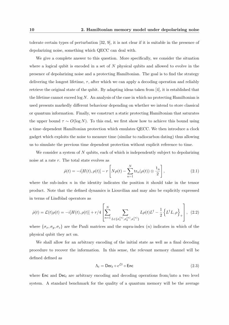
Figure 2.1: Decoding a nested QECC. The “discarded” qubits carry most of the entropy
and are not used further.
concatenated QECC [3, 47, 48] (i.e., l levels of the QECC nested into each other), which
requires N = dl qubits, where d is the number of qubits used by the code. Each level of the
QECC can provide protection for a constant time tprot < tcl, and thus, after tprot one layer
of decoding needs to be executed. Each decoding consists of a unitary Udec on each d-tuple
of qubits in the current encoding level; after the decoding, only one of each of the d qubits is
used further (Fig. 2.1). The total time that such a concatenated QECC can protect a qubit
is given by tprotl = tprot logdN ∼ O(logN), as in the classical case.
2.4 Time-independent protection
In the following, we show that the same logN protection time which we can achieve using a
time-dependent protection circuit can also be obtained from a time-independent protecting
Hamiltonian. The basic idea of our construction is to simulate the time-dependent Hamil-
tonian presented before with a time independent one. To this end, a clock is built which
serves as control. The time-independent version performs the decoding gates conditioned on
the time estimate provided by the clock. In order to obtain a clock from (2.1) with a time-
independent H, we will make use of the noise acting on the system: we add a number, K, of
“clock qubits” which we initialize to |1〉⊗K and let the depolarizing noise act on them. The
behavior of the clock qubits is thus purely classical; they act as K classical bits initialized to
1 which are being flipped at a rate r/2. Thus, the polarization k, defined by the number of
“1” bits minus the number of “0” bits has an average expected value of k(t) = Ke−rt at time
14 2. Hamiltonian memory model under depolarizing noise
t. Conversely, this provides the time estimate
t(k) = min
(ln(K/k)
r, tmax
). (2.6)
Particular realizations of this random process of bit flips can be described by a polarization
trajectory k(t). Good trajectories are defined to be those such that
|k(t)− k(t)| < K1/2+ε (2.7)
for all 0 ≤ t ≤ tmax. For appropriate parameters tmax and 0 < ε < 12 , the following theorem
states that almost all trajectories are good and can provide accurate time estimates.
Theorem 2.4.1 (Depolarizing clock) For K ≥ 16, good trajectories have a probability
P [k(t) good traj.] ≥ 1−Krtmax + exp[−3K2ε/8]
exp[K2ε/8]. (2.8)
Furthermore, for any good trajectory k(t), the time estimate t returned by the clock will differ
from the real time t by at most
δ
2:=
1
rK1/2−ε ertmax ≥ |t(k(t))− t| . (2.9)
Note that the theorem does not simply state that any time evolution will be outside (2.7)
for an exponentially small amount of time (which is easier to prove), but that there is only
an exponentially small number of cases in which (2.7) is violated at all. Although the former
statement would in principle suffice to use the clock in our construction, the stronger version
of the theorem makes the application of the clock, and in particular the error analysis, more
transparent and will hopefully lead to further applications of the clock gadget.
Proof. To prove the theorem, note that each of the bits undergoes an independent exponential
decay, so that the total polarization is the sum of K identical independent random variables.
We can thus use Hoeffding’s inequality [58] to bound the probability of finding a polarization
far from the expected average value k(t),
Pr[|k(t)− k(t)| ≥ K1/2+ε
]≤ 2e−
K2ε
2 . (2.10)
This already implies that most of the trajectories violate (2.7) for no more than an ex-
ponentially small amount of time. To see why (2.10) implies that most trajectories are good
trajectories, we bound the average number of times a trajectory leaves the region (2.7) of
2.4 Time-independent protection 15
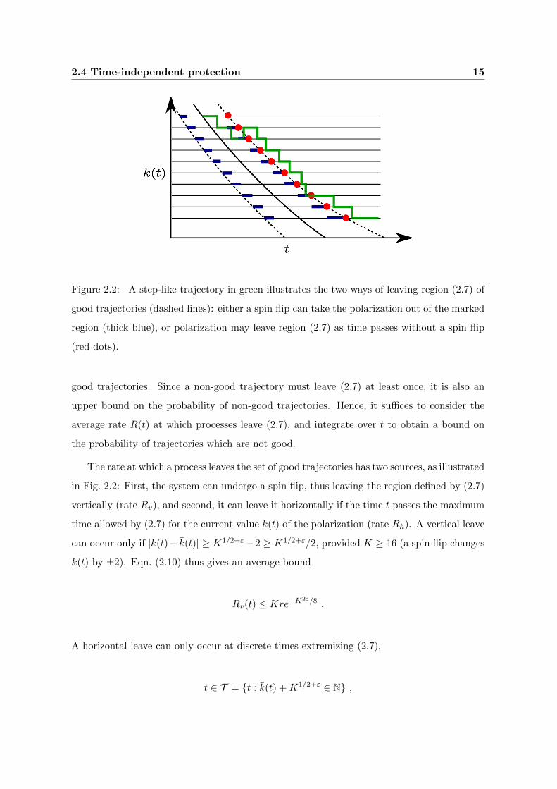
Figure 2.2: A step-like trajectory in green illustrates the two ways of leaving region (2.7) of
good trajectories (dashed lines): either a spin flip can take the polarization out of the marked
region (thick blue), or polarization may leave region (2.7) as time passes without a spin flip
(red dots).
good trajectories. Since a non-good trajectory must leave (2.7) at least once, it is also an
upper bound on the probability of non-good trajectories. Hence, it suffices to consider the
average rate R(t) at which processes leave (2.7), and integrate over t to obtain a bound on
the probability of trajectories which are not good.
The rate at which a process leaves the set of good trajectories has two sources, as illustrated
in Fig. 2.2: First, the system can undergo a spin flip, thus leaving the region defined by (2.7)
vertically (rate Rv), and second, it can leave it horizontally if the time t passes the maximum
time allowed by (2.7) for the current value k(t) of the polarization (rate Rh). A vertical leave
can occur only if |k(t)− k(t)| ≥ K1/2+ε−2 ≥ K1/2+ε/2, provided K ≥ 16 (a spin flip changes
k(t) by ±2). Eqn. (2.10) thus gives an average bound
Rv(t) ≤ Kre−K2ε/8 .
A horizontal leave can only occur at discrete times extremizing (2.7),
t ∈ T = {t : k(t) +K1/2+ε ∈ N} ,

16 2. Hamiltonian memory model under depolarizing noise
and the probability of a trajectory fulfilling k(t) = k(t)+K1/2+ε may again be bounded using
(2.10), such that
Rh(t) ≤ 2e−K2ε/2
∑τ∈T
δ(t− τ) .
The inequality (2.8) follows immediately by integrating Rh(t) +Rv(t) from 0 to tmax.
Assuming that k(t) corresponds to a good trajectory, the accuracy of the time estimate
(2.6) may be bounded by applying the mean value theorem to k:
|t(k(t))− t| = |k(t(k(t)))− k(t)||k′(tinterm)| ≤ Kε
r√Kertmax .
2.4.1 Clock dependent Hamiltonian
Let us now show how the decoding circuit can be implemented using the clock gadget. The
circuit under consideration consists of the decoding unitaries U l,kdec (decoding the k’th encoded
qubit in level l, acting on d qubits each); after a time interval tprot (the time one level of the
code can protect the qubit sufficiently well), we perform all unitaries U l,kdec at the current level
l—note that they act on distinct qubits and thus commute. Each of these unitaries can be
realized by applying a d-qubit Hamiltonian H l,kdec for a time t = tdec. Thus, we have to switch
on all the H l,·dec for t ∈ [tl, tl + tdec], where tl = l tprot + (l − 1)tdec.
In order to control the Hamiltonian from the noisy clock, we define clock times kl,on =
bk(tl)c and kl,off = dk(tl + tdec)e, and introduce a time-independent Hamiltonian which turns
on the decoding Hamiltonian for level l between k ∈ [kl,on, kl,off ],
H =∑l
(H l,1
dec + · · ·+H l,dL−l
dec
)⊗Πl . (2.11)
The left part of the tensor product acts on the N code qubits, the right part on the K clock
(qu)bits, and
Πl =
kl,off∑k=kl,on
∑wx=(k+N)/2
|x〉 〈x| ,
where x is an N -bit string with Hamming weight wx. The initial state of the system is, as
for the circuit construction, the product of the encoded qubit in an l-level concatenated code
and the maximally polarized state |1〉⊗K on the clock gadget.
2.4 Time-independent protection 17
2.4.2 Error analysis
We now perform the error analysis for the protecting Hamiltonian (2.11). In order to protect
the quantum information, we will require that the error probability per qubit in use is bounded
by the same threshold p∗ after each decoding step is completed (i.e. at t = tl + tdec + δ2). We
will restrict to the space of good trajectories, since we know from the clock theorem that this
accounts for all but an exponentially small fraction, which can be incorporated into the final
error probability.
We will choose K large enough to ensure that the error δ2 ≥ |t − t| in the clock time
satisfies δ � tprot, tdec. In this way, we ensure that the decoding operations are performed in
the right order 1 and with sufficient precision. We may thus account for the following error
sources between tl + tdec + δ/2 and tl+1 + tdec + δ/2:
i) Inherited errors from the previous rounds which could not be corrected for. By assump-
tion, these errors are bounded by pinher ≤ p∗.ii) Errors from the depolarizing noise during the free evolution of the system. The system
is sure to evolve freely for a time tprot − δ, i.e., the noise per qubit is bounded by pevol ≤1− exp[−r(tprot − δ)] ≤ r(tprot − δ).
iii) Errors during the decoding. These errors affect the decoded rather than the encoded
system and stem from two sources: On the one hand, the time the Hamiltonian is active has
an uncertainty tdec ± δ, which gives an error in the implemented unitary of not more than
exp[δ‖Hk,ldec‖] − 1. On the other hand, depolarizing noise can act during the decoding for at
most a time tdec + δ. In the worst case, noise on any of the code qubits during decoding
will destroy the decoded qubit, giving an error bound d(1− exp[−r(tdec + δ)]) ≤ dr(tdec + δ).
Thus, the error on the decoded qubit is
pdec ≤ exp[‖Hk,ldec‖δ]− 1 + dr(tdec + δ) .
Since the noise is Markovian (i.e. memoryless), the clock does not correlate its errors in time.
In summary, the error after one round of decoding is at most B(pinher + pevol) + pdec, which
we require to be bounded by p∗ again. Here, B(p) is a property of the code, and returns the
error probability of the decoded qubit, given a probability p of error on each of the original
qubits; for example, for the 5-qubit perfect QECC [80], B(p) ≤ 10p2.
1The noisy clock has the potential to run backwards in time within its accuracy.
18 2. Hamiltonian memory model under depolarizing noise
We will now show that it is possible to fulfil the required conditions by appropriately
defining the control parameters. First, we choose p∗ ≤ 1/40 to have the QECC [80] work well
below threshold. We may take tprot := p∗
r and tdec := p∗
4dr . To minimize imprecision in the
implemented unitaries, the decoding Hamiltonians are chosen of minimal possible strength,
‖Hk,ldec‖ ≤ 2π
tdec. Finally we take δ := p∗tdec
8π . Inserting the proposed values in the derived
bounds, it is straightforward to show that B(pinher + pevol) + pdec < p∗.
The number of code qubits required is N := dl, with l := d τtprot+tdec
e. The required clock
lifetime tmax = τ and precision δ are guaranteed by taking ε = 1/6 and K := (2erτ
rδ )3 in the
clock theorem. For any fixed r and p∗, this allows a lifetime τ ∼ O(log(N +K)).
2.5 Conclusions
In this chapter, we have considered the ability of a Hamiltonian to protect quantum in-
formation from depolarizing noise. While without a Hamiltonian, quantum information is
destroyed in constant time, the presence of time-dependent control can provide protection for
logarithmic time, which is optimal. As we have shown, the same level of protection can be
attained with a time-independent Hamiltonian. The construction introduced a noise-driven
clock which allows a time dependent Hamiltonian to be emulated without explicit reference
to time.
Since depolarizing noise is a limiting case of local noise models, it is expected that the time-
independent Hamiltonian developed here can be tuned to give the same degree of protection
against weaker local noise models, although these models may admit superior strategies. For
instance, noise of certain forms (such as dephasing) allows for storage of ancillas, potentially
yielding a linear survival time by error correcting without decoding. In the case of amplitude
damping noise, the noise itself distills ancillas so that the circuit can implement a full fault-
tolerant scheme, which gives an exponential survival time, assuming that one can redesign
the clock gadget to also benefit from these properties.
Whether the same degree of protection can be obtained from a Hamiltonian which is local
on a 2D or 3D lattice geometry remains an open question2. However, intuition suggests this
2A first step is to incorporate the notion of boundedness. By controlling each decoding unitary in a given
round from a different clock (which does not affect the scaling properties), a constant bound to the sum of
Hamiltonian terms acting on any given finite subsystem can be shown.
2.5 Conclusions 19
might be impossible; the crucial point in reversibly protecting quantum information from
depolarizing noise is to concentrate the entropy in one part of the system. Since the speed of
information (and thus entropy) transport is constant due to the Lieb-Robinson bound [83],
the rate at which entropy can be removed from a given volume is proportional to its surface
area, while the entropy increase goes as the volume. It thus seems impossible to remove the
entropy sufficiently quickly, although this argument is not fully rigorous, and the question
warrants further investigation.

20 2. Hamiltonian memory model under depolarizing noise

Chapter 3
Hamiltonian memory model under
Hamiltonian perturbations
In this chapter, we study limitations on the asymptotic stability of quantum
information stored in passive N-qubit systems. We consider the effect of small
imperfections in the implementation of the protecting Hamiltonian in the form
of Hamiltonian perturbations or weak coupling to a ground state environment.
We thus depart from the usual Markovian approximation for a thermal bath
by concentrating on models for which part of the evolution can be calculated
exactly. We prove that, regardless of the protecting Hamiltonian, there exists a
perturbed evolution that necessitates a final error correcting step for the state
of the memory to be read. Such an error correction step is shown to require a
finite error threshold, the lack thereof being exemplified by the 3D XZ-compass
model [11]. We go on to present explicit weak Hamiltonian perturbations which
destroy the logical information stored in the 2D toric code in a time O(log(N)).
3.1 Introduction
Quantum information processing promises exciting new capabilities for a host of computa-
tional [114, 28, 56] and cryptographic [16, 37] tasks, if only we can fabricate devices that
take advantage of the subtle and very fragile effects of quantum mechanics. The theory of
quantum error-correcting codes (QECCs) and fault-tolerance [113, 3, 47, 48] assure that this

22 3. Hamiltonian memory model under Hamiltonian perturbations
fragility can be overcome at a logical level once an error rate per element below a certain
threshold is achieved. However, providing a scalable physical implementation of computa-
tional elements with the required degree of precision and control has proven to be a task of
extreme difficulty. Thus, one might hope to design superior fault-tolerant components whose
robustness is enforced in a more natural way at a physical level.
A first step in this daunting task is to concentrate not on universal quantum computation,
but on one sub-protocol within this; the storage of quantum information. Thus, the aim is
to find systems naturally assuring the stability of quantum information, just like magnetic
domains in a hard disk provide stable storage of classical information. The quest for such a
passive quantum memory was pioneered by Kitaev [74], who introduced the toric code as the
first many body protecting Hamiltonian. The promising conjunction of properties shown by
his proposal has fueled a search, which is yet to provide a definitive result.
For families of protecting Hamiltonians, such as Kitaev’s toric code [74, 32], a constant
energy gap γ separates the degenerate ground space, used for encoding, from low energy
excited states. Furthermore, the stabilizer representation of these Hamiltonians naturally
associates it with a QECC, which permits an error threshold without the use of concatenation
[32]. A perturbation theoretic expansion of local errors V in the Hamiltonian must then cancel
to orders increasing with the distance of the associated QECC. Recently Bravyi et al. [21, 20]
have used this to rigorously prove that under the effect of sufficiently weak yet extensive
perturbations, the energy splitting of the degenerate ground space decays exponentially with
the system size. Together with previous results by Hastings and Wen [57], this guarantees
the existence of perturbed logical operators and local observable. Additionally, it also implies
that it takes this splitting an exponentially long time to implement logical rotations on the
perturbed ground space (e.g. a phase gate). A non trivial condition being that encoding is
actually performed onto the perturbed ground space.
However, such perturbation theoretic results must be applied with caution. The most im-
portant limitation probably arises from the fact that they deal with a closed quantum system
whereas actual noise may be better modeled by perturbative coupling to an environment.
Even if local observables can be adapted for to a high degree of accuracy [57], the global
eigenstates of the system may change and become very different. Within our understand-
ing, the possibility of adapting encoding and decoding protocols relies on the perturbation
3.1 Introduction 23
being characterized, something that seems unrealistic for such many-body systems1. This
is why we consider an uncharacterized perturbation introduced through a quench. By this
we mean that encoding is performed according to the ideal (unadapted) code-space of the
unperturbed Hamiltonian as will the decoding and order parameters considered. This allows
us to derive no-go, or limitation, results from the exact analysis of adversarially engineered
noise instances. However, it must be noted that error correction to the perturbed encoding
may be performed without explicit knowledge of the perturbation. This is for example the
case, for the self-correcting mechanism which is based on energy dissipation.
The first systematic study of limitations of passive quantum memories can be atributed
to Nussinov and Ortiz [99], finding constant (system size independent) bounds for the auto-
correlation times. They study the effect of infinitesimal symmetry breaking fields on topolog-
ical quantum order at finite temperature [100]. More recently, Alicki et. al. have presented
results supporting the thermal instability of quantum memories based on Kitaev’s 2D toric
code [8] and the stability of its 4D version [9] when coupled to a sufficiently cold thermal
environment. They analyse the evolution of correlation functions for the case of Markovian
dynamical semigroup [7]. Chesi et al. [26] have made progress in providing a general expres-
sion giving a lower bound for the lifetime of encoded information. The approach taken in
these articles is thermodynamic in nature and has the advantage of allowing the derivation
of positive results. A weak coupling Markovian approximation to an environment at thermal
equilibrium is assumed, thus neglecting any memory effects from the environment. In a pre-
vious article [103], we considered a Hamiltonian system subject to independent depolarizing
noise (corresponding to the infinite temperature limit of the above approach) and proved that
O(logN) is the optimal survival time for a logical qubit stored inside N physical qubits.
Our current approach directly deals with Hamiltonian perturbations and environment
couplings without going through a Markovian approximation for the environment. Thus,
approximations needed for a Markovian description of a bath are not required and do not
pose an issue. A comparative advantage of our approach is the capability of exactly dealing
with certain weak but finite perturbations and couplings, and providing restricted no go
results.
To falsify claims of protection against any possible noise of a certain class (such as weak
1A possible exception to this is given by proposals of adiabatic state preparation [54].

24 3. Hamiltonian memory model under Hamiltonian perturbations
local perturbations to the Hamiltonian), it suffices to consider an adversarial noise instance
within such a class. In such a noise model, different perturbations and environments are not
assigned probabilities; a perturbation is simply considered possible if it adheres to certain
conditions. There is a range of different conclusions that one may reach from such an analysis
of noise instances. One may simply provide upper bounds on how fast a passive memory may
be erased by a perturbation complying to a certain noise class. We may prove or extrapolate
requirements for a memory model to protect against the given noise class. We may find that a
class of noise is unreasonable by showing that it invalidates a memory model which we expect
to work (i.e. a magnetic domain). An intermediate scenario arises when we consider the
noise class to be reasonable but expect a certain notion of typicality for which the considered
instance is not representative. Such a typicality condition would then be needed explicitly to
provide proof of robustness for the memory model.
We consider the effect of relatively weak yet unknown perturbations of an N qubit local
protecting Hamiltonian and coupling to an ancillary environment starting out in its ground
state. We show that as the number N of physical subsystems used grows, it is impossible to
immunize a quantum subspace against such noise by means of local protecting Hamiltonians
only. We further show that if one wishes to recover the quantum state by means of an error
correction procedure, the QECC used must have some finite error threshold in order to guar-
antee a high fidelity; this result is applied to the 3D XZ-compass model [11] which is shown
not to have such a threshold. In the case of the 2D toric code [74], we propose Hamiltonian
perturbations capable of destroying encoded information after a time proportional to log(N),
suggesting that some form of macroscopic energy barrier may be necessary. Weak finite range
Hamiltonian perturbations are then presented which destroy classical information encoded
into the 2D Ising model; in this case interactions involving a large, yet N independent, num-
ber of qubits are required. Finally, we consider time dependent Hamiltonian perturbations
and coupling to an ancillary environment with a high energy density; here we provide con-
structions illustrating how these more powerful models may easily introduce logical errors in
constant time into information protected by any stabilizer Hamiltonians, and even certain
generalizations. Drawing from practical experience with classical memories, the one likely
conclusion here is that general time dependent Hamiltonian perturbations are not a relevant
noise model to consider, as it is in general too powerful to protect against.

3.1 Introduction 25
3.1.1 Noise model motivation
A prerequisite to assess protecting Hamiltonians is a precise definition of the noise model
they will be expected to counter. Our aim is to understand the protection lifetime they
provide to (quantum) information as well as to identify the properties a good protecting
Hamiltonian should have. In order to be able to make such predictions, we will study noise
models admitting a mathematically tractable description while striving to keep our choices
physically motivated.
The most elementary way in which the Hamiltonian evolution of a closed system can
be altered is by including a small perturbation V to the Hamiltonian H. A simple physical
interpretation for such a perturbation is to associate V to imperfections in the implementation
of the ideal protecting Hamiltonian H. Furthermore, Hamiltonian perturbations extending
beyond the system under experimental control are modeled by a weak coupling between
the system and an environment. We focus on families of protecting Hamiltonians satisfying
certain locality and boundedness conditions, and naturally extend similar restrictions on the
perturbations and couplings considered.
Let us first introduce some definitions. A family of protecting Hamiltonians {HN} is
parametrized by a natural number N which in most cases, will simply be the number of
physical subsystems (particles) on which HN acts. A Hamiltonian H is called “k-local” when
it can be represented as a sum
H =∑i
Ti, (3.1)
with at most k physical subsystems participating in each interaction term Ti. The interaction
strength of a physical subsystem s in a k-local Hamiltonian H is given by the sum∑
i |Ti| of
operator norms over those interaction terms Ti in which the physical subsystem s participates.
A family of k-local Hamiltonians is called “J-bounded” if, for every Hamiltonian HN in the
family, the largest interaction strength among the physical subsystems involved is no greater
than J . Finally, a family of Hamiltonians will be D-dimensional if the physical subsystems
involved can be arranged into a D-dimensional square lattice, such that all interaction terms
are kept geometrically local.
We will concentrate on families of k-local, J-bounded protecting Hamiltonians, with J > 0,
and k, J ∼ O(1). Furthermore, the specific Hamiltonians treated in this chapter admit an
embedding into 2, 3 or 4 spatial dimensions and we may assume such embeddings also when
26 3. Hamiltonian memory model under Hamiltonian perturbations
dealing with generic protecting Hamiltonians.
The families of Hamiltonian perturbations {VN} which we will consider will be J-bounded,
with the strength J small in comparison to J . The perturbations will be taken to be k-local,
with k possibly different, and even larger, than k. This allows, for example, taking into
consideration undesired higher order terms which may arise from perturbation theory gadgets
[19]. Allowed perturbations should also admit a geometrically local interpretation under the
same arrangement of subsystems as the protecting Hamiltonian.
When considering coupling to an environment, an additional set of physical subsystems
will be included as the environment state. A family of local environment Hamiltonians {H(E)N }
will be defined on these additional subsystems. The coupling between system and environment
will be given by a family of weak local Hamiltonian perturbations V(SE)N , acting on both
system and environment.
HN = H(S)N ⊗ I(E)
N + I(S)N ⊗H(E)
N + V(SE)N (3.2)
Finally, it should be possible to incorporate the additional physical subsystems from the
environment while preserving the number of spatial dimensions required for the Hamiltonian.
To simplify notation, the sub-index N shall in general be dropped.
The engineering of k-body interactions is increasingly difficult as k grows [130, 19]. This is
why we limit our study to families of k-local Hamiltonians (i.e. k independent ofN). It is under
such criteria that we exclude proposals such as quantum concatenated-code Hamiltonians
[12], for which the required degree of interactions would grow algebraically with the number
of qubits.
The J-bounded condition guarantees that the rate of change for local observables remain
bounded. This is a necessary condition to certifiably approximate a Hamiltonian through
perturbation theory gadgets [19]. There, constant bounds are imposed both on the norm of
each interaction as well as on the number of interactions in which each subsystem partici-
pates. The J-bounded condition also leaves out systems with long range interactions, as, for
those systems, the total interaction strength of individual physical subsystems diverges as the
system size grows. Such long range interacting systems are physically relevant, and may lead
to protecting Hamiltonian proposals [27, 53]. However, we abstain from treating such models
for which our notion of weak perturbation seems inappropriate.

3.1 Introduction 27
Each physical subsystem may independently be subject to control imprecision. Such is
the case for weak unaccounted “magnetic field” acting on every component of the system or
a weak coupling of each component to an independent environment. Thus, relevant physical
scenarios involve perturbations with extensive operator norm (i.e. scaling with the number
of subsystems). The J-bounded condition encapsulates these scenarios and seems to better
describe what we understand by a weak perturbation.
Finally, it is expected that scalable physical implementations should be mapped to at most
three spatial dimensions. This would rule out the 4D toric code Hamiltonian [32], a proposal
which was otherwise shown to provide increasing protection against weak local coupling to
a sufficiently cold thermal bath [9]. As would occur with an actual physical embedding, we
expect that the perturbations considered may be included into the same geometrical picture
as the protecting Hamiltonian they affect.
3.1.2 Outline of results
In the following sections, we analyze the problem of obtaining increased protection for quan-
tum information by means of an encoding and a protecting Hamiltonian acting on an in-
creasing number of physical subsystems. We consider the effect of adversarial noise models
consisting of local Hamiltonian perturbations and/or a weakly coupled environment. The
aim is to examine the assumptions and limitations of memory schemes based on Hamiltonian
protection with a growing number of physical subsystems as quantified by the survival time
of stored information.
We will prove in complete generality that the survival of information should be associ-
ated to a subsystem and not to a particular subspace. The figure of merit considered here
is S(t) = tr (|ψ(0)〉 〈ψ(0)| ρ(t)), the overlap between initial and evolved state after a constant
time t. For arbitrary protecting Hamiltonians we provide a completely general construction
involving a weakly coupled environment starting in its ground state (Sec. 3.2.2) which yields
an exponentially small (in N) upper bound on S(t) after a constant time. For gapped Hamil-
tonians, a proof proceeding without reference to an environment (Appendix 3.A) can provide
an upper bound to the time averaged overlap which is close to 12 . We thus infer that the
information should be associated to a subsystem.
Having found that subspaces can not provide robust encoding, we consider protecting
28 3. Hamiltonian memory model under Hamiltonian perturbations
Hamiltonians together with a recovery operation R, which can be thought of as applied on
read-out. This provides the formal means to project information from a logical subsystem onto
a code subspace and leads to a more robust figure of merit given by SR(t) = tr (ρ(0)R(ρ(t))).
Although throughout the chapter, we assume R to be an unperturbed error correction pro-
cedure associated to an encoding, it is important to emphasize that other means may allow
keeping information in a logical subsystem. In particular, self-correcting Hamiltonians advo-
cate the use of a local thermalizing coupling as a way of continuous error correction at finite
temperature. This is, while an unperturbed order parameter may be shown to be inadequate
for the storage of information, it may be possible for a robust yet implicit logical subsystem
to arise by including genuine dissipation.
In (Sec. 3.3), a weak coupling construction like that of (Sec. 3.2.2) shows that information
content of the 3D XZ-compass model [11] can be destroyed in constant time by a zero tem-
perature environment, despite of a final recovery operation R. From a broader perspective,
the structure of our proof strongly suggests that the underlying QECC defining the recovery
operation R must have a strictly positive error threshold.
We continue by considering the effect of Hamiltonian perturbations on the 2D toric code
[74]. The recovery mechanism R is then taken as the composition of a fixed syndrome mea-
surement followed by a correction operation pairing the detected anyons. It is shown (Sec. 3.4)
that, although the underlying QECC has an error threshold, it is not protected against com-
binations of unknown weak local Hamiltonian perturbations, even after a final round of error
correction is considered. Our claim is based on adversarial weak local perturbations that are
capable of destroying the stored information in a time logarithmic in N . This is stronger than
previous results [67] in that, the noise model requires no interaction with the environment
and the information is destroyed exponentially faster.
In a similar manner, we consider perturbations on the 2D Ising Hamiltonian (Sec. 3.5),
which is often used as an example of self-correcting classical memory. Here, Hamiltonian
perturbations may transform (classical) code states into an ambiguous state in constant time.
While the number k of bodies in perturbation terms is required to grow as the overall pertur-
bation strength decreases, it shows no dependence on the size N of the system. In this model,
any sequence of local errors connecting the two classical code states must go through states
with a macroscopic amount of extra energy, showing that this property alone is not sufficient
3.2 Subsystems instead of subspaces 29
to give protection against this family of perturbations. There are two possible implications
of this result. First we may think that since ferromagnetic domains seem to be quite stable,
our choice of perturbation may not be significant in that it is by no means typical. On the
other hand, although the lifetime obtained is independent of N , this independence is only
found for very large N in terms of the perturbation strength, possibly allowing to reconcile
this model with experience and hinting that in practice, information lifetime scaling with N
may be unnecessary.
Beyond the Hamiltonian perturbation model and coupling to a ground state environment,
we consider more aggressive noise models (Sec. 3.6) in which the environment can introduce
large amounts of energy. The models considered are time dependent Hamiltonian perturba-
tions and weak Hamiltonian coupling to an environment starting in a high energy state. For
such noise models, even the information storage capabilities of the 4D toric code and any local
ferromagnetic Ising model, proposals shown to be stable under Markovian thermal coupling,
are completely destroyed. We thus argue that requiring robustness against an adversarial
noise model of such a class is asking for too much and is not a prerequisite for practical
quantum or classical memories.
One might expect that the results presented here are not limited to the task of designing
a quantum memory. Rather, they tell us about the difficulty of keeping a state and its time
evolution confined within a specific subspace of the system, under the effect of Hamiltonian
noise. Such considerations arise in other settings, such as in the models of adiabatic and
topological quantum computation. We will outline some of these connections in Sec. 3.7.
3.2 Subsystems instead of subspaces
We start our examination of passive quantum memories by proving that regardless of the
choice of encoding subspace and protecting Hamiltonian the weak coupling to an environment
can, in constant time, exponentially reduce the fidelity with the evolved state. By this, we
wish to convey that a more robust figure of merit is required. Such figures are in general
derived from associating the information to a logical subsystem.
First, we propose weak local perturbations showing an exponentially decreasing overlap
between perturbed and unperturbed eigenstates. For general local Hamiltonians and states,
we consider a local coupling V of the system with a γ-bounded environment initialized in its

30 3. Hamiltonian memory model under Hamiltonian perturbations
ground state. Averaging over such couplings V , we are able to derive an exponentially small
upper bound 〈S(tf )〉V ≤ [1 − sin2(2ε)]N for the overlap between initial and evolved system
states at a time tf = πγ .
3.2.1 Eigenstate susceptibility to perturbations
Consider a k-local HamiltonianH, decomposable into k-body interaction terms Ti as described
in (3.1). We choose a perturbation V such that the initial and final Hamiltonians are related
by a composition of local unitary transformations,
H = H + V = UHU†, with U =N⊗l=1
eiεPl , (3.3)
where Pl are normalized local Hermitian operators. Taking this definition, V can be written
as
V =∑i
UTiU† − Ti, (3.4)
and thus is also k-local. Furthermore, if 2kε� 1, it is justified to call V a perturbation with
respect to H, since all terms are small with respect to those of H.
Degeneracies in H are assumed to be infinitesimally lifted to ensure uniquely defined
eigenvectors. The overlap between eigenvectors |ψi〉 of H and the perturbed eigenvectors
U |ψi〉 is then given by FU = |〈ψi| U |ψi〉|2.
By averaging over all possible directions Pl, we effectively obtain an independent qubit
depolarization. ∫U† |ψi〉 〈ψi| UdP1 . . . dPN = ∆⊗Nλ(ε)(|ψi〉 〈ψi|) (3.5)
Here, ∆λ(ρ) = λρ+ (1− λ) I2 is the qubit depolarizing channel and λ(ε) = 1− 32 sin2(ε). We
may then denote 〈F 〉U as average of the overlap FU over all local rotations U having a given
strength ε. This average is expressed in terms of the depolarizing channel as
〈F 〉U = 〈ψi|∆⊗Nλ(ε) (|ψi〉 〈ψi|) |ψi〉 . (3.6)
A result of King [72], known as multiplicativity of the maximum output p-norm for the
depolarizing channels, states that
max|φ〉
∣∣∣∆⊗Nλ (|φ〉 〈φ|)∣∣∣p≤(
max|φ〉|∆λ (|φ〉 〈φ|)|p
)N. (3.7)
3.2 Subsystems instead of subspaces 31
For qubit subsystems and for p =∞, Eq. (3.7) bounds the overlap of ∆⊗Nλ (|φ〉 〈φ|) with any
single pure state, leading to
〈F 〉U ≤(
1 + λ
2
)N=
(1− 3
4sin2(ε)
)N. (3.8)
Not only does this imply the existence of specific rotations such that F becomes exponentially
small as the number of subsystems N grows, but that this is true for most rotations U .
While this is already known under the name of Anderson’s orthogonality catastrophe (see,
for example [10, 124]), we re-derive it for completeness and as an opportunity to introduce
techniques needed throughout the rest of the chapter.
3.2.2 State evolution in coupled Hamiltonians
In this section, we consider a weak Hamiltonian perturbation coupling the system to a “cold”
environment. The environment is assumed to start in its ground state, corresponding to a cold
environment assumption. Averaging over a specific family of such perturbations instances V ,
an exponentially small bound on the overlap between the initial state and the evolved state
is obtained. This bound, 〈S(tf )〉V ≤ [1− sin2(2ε)/3]N , is obtained after a constant evolution
time tf = πγ , inversely proportional to the strength of the environment Hamiltonian.
Suppose that we start with a state |ψ0〉 “protected” by an N qubit system Hamiltonian
HS . We can introduce a simple environment, composed of 2N qubits, each of which starts in
its ground state, |0〉, and which is defined by its Hamiltonian
H = H(S) ⊗ I(E) + I(S) ⊗H(E) (3.9)
H(E) = γ
N∑i=1
|1+〉〈1+|(E)i − |00〉〈00|(E)
i . (3.10)
When necessary, we take the supraindices (S), (E1) and (E2) to denote the system, the first,
and second components of the environment respectively. While both environment components
will interact with the system, it is the presence of both which will allow a simple interpretation
of the induced decoherence as a probabilistic application of local errors.
We again use the trick of considering a perturbed Hamiltonian H = UHU† which results
from the weak local rotations U =⊗N
j=1 Uj of the decoupled Hamiltonian H. The rotation
elements will involve both system and environment components, Uj = eiεP(S)j ⊗X(E1)
j , where
the operators P(S)j are taken to be Pauli-like operators on site j of the system.

32 3. Hamiltonian memory model under Hamiltonian perturbations
The perturbation V = UHU† − H must be decomposable into small local terms. Such
a decomposition for V is given in terms of the decomposition H(S) =∑
i Ti into at most
k-body terms. Each perturbation term Vi = UTiU† − Ti has an operator norm no greater
than 2εk |Ti| and involves up to 2k-body interactions2. The perturbation required to rotate
the environment Hamiltonian terms involve at most 3-body terms and a total norm bounded
by 2εγ.
The initial state, |ψ0〉 |00〉⊗N will thus evolve into e−itUHU† |ψ0〉 |00〉⊗N . The survival
probability is then S(t) = 〈ψ0| ρS(t) |ψ0〉, where ρS(t) = trE (ρ(t)), and
ρ(t) = Ue−itHU† |ψ0〉〈ψ0| ⊗ |00〉〈00|⊗N UeitHU†. (3.11)
Here, U may be explicitly decomposed as
U = exp(iε∑
j P(S)j ⊗X(E1)
j )
=∑
p cos(ε)N−w(p)(i sin(ε))w(p)P(S)p ⊗X(E1)
p ,(3.12)
where p denotes a binary vector indicating the sites on which rotations are applied in P(S)p
and w(p) is the weight of the bit string p (number of non identity factors in P(S)p ).
Now consider a time tf = πγ such that e−itfH transforms components of the environment
from |10〉 to |11〉, while leaving components in state |00〉 unaltered. At such a time tf ,
substituting U into expressions (3.11) allows explicitly tracing over the environment to yield
ρS(tf ) =∑p,q
cos2(ε)2N−w(p)−w(q) sin2(ε)w(p)+w(q)×
Ppe−itfH(S)
Pq |ψ0〉〈ψ0|PqeitfH
(S)Pp.
(3.13)
Thus, ρS(tf ) may be considered as the density matrix resulting from the independent proba-
bilistic application of the local unitary rotations prescribed by U on |ψ0〉〈ψ0|, followed by the
evolution under the unperturbed system Hamiltonian, followed by a second round of random
application of the local rotations prescribed by U . Defining
ER,p(ρ) = pRρR+ (1− p)ρ, (3.14)
and the Hamiltonian evolution
Ht(ρ) = e−iH(S)tρeiH
(S)t, (3.15)
2For εk � 1, a further decomposition of such terms can be provided in which subterms involving k + b
bodies are of strength O(εb), guaranteeing that the strength of terms decays exponentially with the number
of bodies involved.
3.2 Subsystems instead of subspaces 33
we can take p = sin2(ε) and define ρvirt :=(⊗N
i=1 EPi,p)|ψ0〉〈ψ0|, so that we can express
S(tf ) as
S(tf ) = tr(ρvirte
−itfHSρvirteitfHS
). (3.16)
This is the overlap between a density matrix and its own unitary evolution, and can be upper
bounded by
S(tf ) ≤ tr(ρ2virt
). (3.17)
In turn, using the fact that Pi are Pauli-like operators we may rewrite it as
S(tf ) ≤ 〈ψ0|(
N⊗i=1
EPi,2p(1−p))
(|ψ0〉〈ψ0|) |ψ0〉 . (3.18)
Averaging over the Pauli-like operators, we obtain
〈S(tf )〉V ≤ 〈ψ0|∆⊗Nλ(ε)(|ψ0〉〈ψ0|) |ψ0〉 , (3.19)
which is the overlap at time tf averaged over the proposed family of weak perturbative
couplings. Here ∆λ(ρ) is again the depolarizing channel, and λ(ε) = is 1− 432p(1− p). Using
Eq. (3.8), we obtain
〈S(tf )〉V ≤ [1− 4
3p(1− p)]N , (3.20)
which by substituting p for sin2(ε) yields
〈S(tf )〉V ≤ [1− sin2(2ε)/3]N . (3.21)
By averaging over different possible weak couplings, we obtain an overlap between initial and
evolved states which is exponentially decreasing in N .
The norm γ of Hamiltonian terms in the environment should be bounded, since it is in
part these terms which are rotated by U to introduce a weak coupling between system and
environment. Thus, the proposed evolution time tf = πγ is constant. Furthermore, if one
considers an environment of N semi-infinite chains of coupled two level systems (such as
Heisenberg chains), it is possible to ensure that the overlap with the initial state is small for
all times larger than t ∼ πγ , rather than have the recurrences that arise from the discrete
spectra of the described model.
In appendix (3.A), the evolution of an unperturbed eigenstate is considered under the
effect of pure Hamiltonian perturbations (no environment). In this case, a constant rate of

34 3. Hamiltonian memory model under Hamiltonian perturbations
change in the system state is guaranteed by an energy gap γ in the system Hamiltonian. If an
initial state belongs to an energy band separated from the rest of the Hilbert space by such an
energy gap γ, we provide an upper bound on the time averaged overlap 〈S(t′)〉t′∈[0,t] ≤ 12 + 1
2γt
between initial and evolved state.
3.2.3 Discussion
We were able to show after a constant time tf , an exponentially large degradation of the over-
lap S(tf ) in terms of N . If we are to find a benchmark by which to evaluate a memory scheme,
we expect that the memory improves as more resources are dedicated to its implementation.
It is now clear that many-body quantum states are inherently unstable with respect to the
uncorrected overlap, i.e. S(t) is not the appropriate benchmark.
The fact that we may count on N physical subsystems to implement a quantum memory
should not exclude using only one of them and ignoring whatever noisy evolution is affecting
the others. This corresponds to considering an overlap reduced to the relevant subsystem
and not on the whole state. Already such a simple idea guarantees that information storage
quality is non-decreasing with N .
One may further generalize this by realizing that the relevant subsystem need not corre-
spond to an actual physical subsystem. This corresponds to providing a new decomposition
for the physical Hilbert space which allows factoring out a logical subsystem. The resulting
benchmark is SR(t) = tr (ρ(0)R(ρ(t))), quantifying the quality of the information recoverable
from the evolved state and not of the state itself. Here, R may be thought of as an operation
zeroing the irrelevant subspace, which may also be interpreted as the recovery super-operator
of a QECC. Conversely, given the recovery operation R of a QECC, one may define the cor-
responding logical subsystem. Robust error corrected logical observables3 can analogously
be defined via the extension provided from the code space to the whole Hilbert space by the
recovery operation R. In the following sections, we shall consider protecting Hamiltonians
toghether with such error correcting codes and robust logical observables.
3 Alicki et al. [9] use the name dressed observables, whereas Chesi et al. [26] use the self-explanatory name
of error corrected logical operators, which we will adopt.

3.3 Error threshold required 35
3.3 Error threshold required
A desirable property for a quantum memory is that any sequence of local operators mapping
between different logical code-states should have energy penalties which grow with the system
size. It has been shown that this happens for schemes in four dimensions, such as the 4D toric
code [32]. Seeking to provide such an example in three spatial dimensions, Bacon proposed
the 3D XZ-compass model [11], a scheme based on subsystem error correcting codes [77] and
requiring only 2-body nearest neighbour interactions. Furthermore, mean field arguments
suggest that this model might show such an increasingly large energetic barrier.
However, we will show that the zero temperature (local, but non-Markovian) environment
construction of the previous section is capable of giving a false read-out from the code after
constant time. A recovery operationR is assumed on read-out, and taken to be the unadapted
version of the associated error correcting code. We show that the shortcoming is inherent to
the choice of recovery procedure R by illustrating that the same flaw is present for the 4D
toric code if one assumes an alternative recovery protocol similar to the one considered for
the 3D XZ-compass model. This failure is a general feature of recovery protocols not having
a local error threshold (i.e. those which are unable to handle errors on a constant fraction of
randomly chosen sites).
For the 3D XZ-compass model, quantum information is first encoded into the groundspace
of a 2-local Hamiltonian HS defined on a N×N×N arrangement of two level systems (where
N is an odd number).
HS = −λN∑
i,j=1
N−1∑l=1
(Xl,i,jXl+1,i,j +Xi,l,jXi,l+1,j
+Zi,l,jZi,l+1,j + Zi,j,lZi,j,l+1) .
(3.22)
This is not a stabilizer code but a subsystem code. This means that a recovery operation need
not correct certain errors which have no effect on the logical observables, and information may
be preserved even if the recovered state is different.
First, note that pairs of planes of operators Zl =∏i,j Zi,j,lZi,j,l+1 and Xl =
∏i,j Xl,i,jXl+1,i,j
commute with the Hamiltonian H for all l. This also holds for logical operators, which con-
sist of products along a single plane Z ≡ Zl =∏i,j Zi,j,l and X ≡ Xl =
∏i,j Xl,i,j operators
respectively, for an arbitrarily chosen l. In the ground space, the choice of l is irrelevant, since
the operators Zl, Xl all have +1 eigenvalues. Provided N is odd, X and Z anti-commute,

36 3. Hamiltonian memory model under Hamiltonian perturbations
giving a qubit algebra. In the presence of errors (outside of the ground space), the error
corrected logical observables will be defined as the majority vote among plane observables
Zec = majlZl Xec = majlXl (3.23)
where maj stands for a majority vote among the ±1 eigenvalued commuting operators. Mea-
suring all pairs of adjacent planes Zl allows a majority vote error correction scheme to be
performed on the value of the Zl plane observables without extracting whether the corrected
state yields +1 or −1 values for all such planes.
Considering a perturbation on the system plus an environment, as presented in section
3.2.2. By explicitly developing the final expectation values for the observables of interest
(tr[ZecρS(tf )] and tr[XecρS(tf )] ), it can be seen that the information stored in the code will
not be reliable after a time tf . For this, we can pick up from the evolved state of the system
in Eq. (3.16)
ρS(tf ) =
(N⊗i=1
EPi,p)◦ Htf ◦
(N⊗i=1
EPi,p)|ψ0〉〈ψ0| . (3.24)
Since all plane observables (Xl and Zl) of a given type mutually commute, and also do so
with the Hamiltonian, we can independently consider the probability of each plane observable
having suffered a flip. If the Pi in Eq. (3.14) are taken to be single X or Z rotations, they will
anticommute with overlaping Zl or Xl plane observables respectively, changing their value
upon an odd number of applications. Taking the Pi to be simple Z operators, the probability
of flipping the value of an Xl plane observables by applying⊗N3
i=1 EPi,p once is given by
pplane∗ =
i≤N∑i∈odd
cos2N2−2i(ε) sin2i(ε)
(N2
i
)
=1− cosN
2(2ε)
2, (3.25)
which is exponentially close to 1/2. Since all observables involved commute with the system
Hamiltonian, the probability of observing any result configuration will be preserved by Htf .
Finally, a second round of errors⊗N3
i=1 EPi,p will again flip the observed value for each plane
with a probability pplane∗. The final independent probability of flipping the value of each
plane is
pplane = 2pplane∗(1− pplane∗) =1− cos2N2
(2ε)
2. (3.26)

3.3 Error threshold required 37
The proposed correction scheme is equivalent to a majority voting among such planes.
Thus, if more than half the planes suffer such an error, the majority vote will fail. The
probability for incorrectly measuring the error corrected logical observable Xec on read-out
is then
plogic =N∑
i=(N+1)/2
piplane(1− pplane)N−i
(N
i
). (3.27)
Given that 12 [1− cos2N2
(2ε)] ≤ pplane ≤ 12 , we have that
1
2[1−N cos2N2
(2ε)] ≤ plogic ≤1
2. (3.28)
Assuming ε to be a small constant independent of N , the probability plogical will exponentially
approach 1/2 for large N . We conclude that the encoding is not robust against the error model
posed by local coupling to a cold adversarial environment.
The problem lies in the error correction mechanism rather than the protecting Hamiltonian
itself. This becomes apparent if one applies a similar analysis to the 4D Toric code. There,
the suggested noise model does not present a problem, since the usual error correction [32] of
the 4D toric code has an error threshold. That is, provided the probability of per-site error,
p = sin2 ε is below this threshold, there exist error correction criteria which succeed with a
probability approaching 1 exponentially with N . On the other hand, we could consider a
majority voting version of error correction in this setting, where we measure hyperplanes of
X operators, and apply a majority vote to choose the correct result. In this case, an analysis
completely analogous to that of the 3D XZ-compass code would hold proving such a read-out
technique unreliable. We conclude that the error correction procedure of the 3D XZ-compass
code does not allow sufficient resolution to use any potentially topological properties of the
encoded quantum information.
The errors introduced by⊗N
i=1 EPi,p are sufficiently general to suggest a necessary crite-
rion for Hamiltonian protection of information from weak coupling to a cold environment.
Even if we consider the first round of errors and the Hamiltonian evolution as part of the
encoding procedure, information should still be able to withstand the probabilistic applica-
tion of arbitrary local errors. This means that the information, either quantum or classical,
should be encoded in such a way as to provide a finite error threshold in the thermodynamic
(large N) limit.

38 3. Hamiltonian memory model under Hamiltonian perturbations
3.4 Limitations of the 2D toric code
We will now show how local Hamiltonian perturbations are capable of introducing uncor-
rectable errors in Kitaev’s 2D toric code Hamiltonian. The introduction of such errors will
strongly rely on the lack of string tension on the toric code, suggesting a macroscopic energy
barrier may be a necessary requirement. A brief introduction to the toric code Hamiltonian
is provided in appendix 3.B, and is recommended to the unfamiliar reader.
Logical operations in the 2D toric code can be realized by creating a pair of anyons,
propagating them so as to complete a non-trivial loop, and finally annihilating them. It is
roughly such a scheme that will be followed by the perturbations we develop here. Repeating
techniques from section 3.2, we may consider the initial state as containing a superposition
of local errors which are interpreted as neighboring anyon pairs. A perturbation construction
due to Kay [67] allows the deterministic propagation of such anyon pairs along predefined
adversarial paths on the lattice. Syndrome measurement allows restricting to a probabilistic
picture where error strings corresponding to anyon propagation paths are present with a
predefined probability. It is finally the recovery procedure which may possibly complete these
errors into logical operations by selecting an incorrect anyon matching.
A family of weak local perturbations capable of probabilistically introducing distant anyon
pairs will first be presented. As before, the initial state |ψ(0)〉 is assumed to be a ground state
of the unperturbed Hamiltonian H, in this case an N ×N toric code as in Eq. (3.63). After
a time tf proportional to the maximum desired anyon propagation distance D, unperturbed
syndrome read-out on |ψ(tf )〉 will probabilistically detect distant (as well as local) anyon
pairs. Our construction will then be applied to produce a simple set of O(N) distance anyons
such that no syndrome based error correction may be reliably applied. Later, shorter yet
more elaborate anyon propagation paths will require explicit analysis of the error correcting
probability of different anyon pairing protocols. In this context, we find weak Hamiltonian
perturbations are capable of introducing logical errors with a large probability (≈ 12) in a
time tf logarithmic in the system size N .
3.4.1 Probabilistic introduction of distant anyons
Kay [67] showed that local errors (anyons) in the 2D toric code, and other local stabilizer
Hamiltonians lacking string tension, can be propagated into logical errors corresponding to
3.4 Limitations of the 2D toric code 39
almost complete loop operators by a local Hamiltonian perturbation P . While in his work
the initial presence of the anyons was assumed, here, anyons will be introduced with a certain
amplitude by a generalization of the Hamiltonian perturbation P .
Consider introducing perturbations of the form V = U(H + P )U† −H, where U =⊗
i Ui
decomposes into weak local unitary rotations, and P is, as in [67], a weak local perturbation
capable of deterministically propagating anyons in a given time tf . The perturbed Hamilto-
nian
H = U(H + P )U† (3.29)
induces a time evolution which can be written as
|ψ(t)〉 = e−itH |ψ(0)〉 = Ue−it(H+P )U† |ψ(0)〉 . (3.30)
In this context, U and P are chosen such that:
1. By applying small Z rotations on connecting edges qubits, pairs of neighbouring vertex
anyon are created by U† with amplitude O(ε).
2. Each of the anyons is deterministically propagated by P along a predefined path. Thus,
local excitation pairs become strings of errors defining new positions for the anyon pair.
3. Finally, U is unable to remove anyon pairs created by U† after at least one of them has
been propagated. Moreover, U may create additional anyon pair with amplitude O(ε).
Propagation paths for each anyon are not allowed to overlap but are otherwise completely
independent. The propagation of the i-th anyon along its path `(i) may be attributed to a
specific component Pi of P =∑
i Pi. In turn, each component Pi admits a decomposition
Pi =
|`(i)|∑j=1
J(i)j T
`(i)j−1,`
(i)j
, (3.31)
in terms of local interaction terms Tp,q, where `(i)j are the anyon locations along the path
`. As in [67], the scalar coefficients J(i)j are chosen to implement a perfect state transfer
[29, 66, 68] and each term Tp,q implement a swap among vertex anyons on p and q. If p and
q are neighboring vertices, Tp,q is defined as
Tp,q = Zs(11−ApAq)
2, (3.32)

40 3. Hamiltonian memory model under Hamiltonian perturbations
where Ap and Aq are the vertex stabilizer operators corresponding to p and q respectively
(appendix 3.B) and Zs is a Z rotation on physical site s corresponding to the edge connecting
p and q. Furthermore, by allowing p and q to be next nearest neighbors, it is possible to have
crossing anyon paths `(j), `(i) without having them overlap in the anyon locations used. If
vertices p and q are not neighbors, the same effect is obtained by substituting Zs in (3.32) for
a tensor product of Z operators along an edge path pq from p to q,
Tp,q =⊗s∈ pq
Zs(11−ApAq)
2. (3.33)
The distance D is the maximum number of steps among the different anyon propagation
paths D = maxi∣∣`(i)∣∣. It will be taken as D = N/2−1 in section (3.4.2) and as D = O(logN)
in section (3.4.4). Fixing the strength of perturbation terms in P as J(i)j = ε
D
√j(∣∣`(i)∣∣+ 1− j)
allows the perturbation P to remain ε-bounded while allowing simultaneous perfect anyon
transfer in a time tf = Dπ2ε . Similarly to previous sections, by taking the rotations Uj = eiεZj as
ε weak, the final perturbation required V will also be composed of O(ε) strength interactions
involving at most 8 bodies each.
The quantum state before measurement at time tf is given in Eq. (3.30). Expanding U†
from Uj = eiεZj , we get
|ψ(tf )〉 = Ue−i(P+H)tf⊗j
(cos ε11j − i sin εZj) |ψ(0)〉 , (3.34)
where the index j ranges over sites of non trivial action for U . The state |ψ(0)〉 is a ground
space eigenstate of H, and assuming the locations j on which U acts are non neighboring,
each Zj will increase the energy respect to H by γ. Furthermore since the energy of a state
respects to H depends only on anyon number and P is anyon number preserving, we have
[H,P ] = 0, allowing us to write
|ψ(tf )〉 = Ue−iP tf⊗j
(cos ε11j − ie−iγtf sin εZj) |ψ(0)〉 . (3.35)
Since all the propagations in P commute and correspond to exact transfer of each anyon
created by U† precisely at time tf , we may write
|ψ(tf )〉 = U∏j
(cos ε11− ie−iγtf sin ε⊗i∈``(j)
Zi) |ψ(0)〉 (3.36)
3.4 Limitations of the 2D toric code 41
where ``(j) is the path given by the union of {j} and the two propagation paths `(j+) and
`(j−) of P corresponding to the each of the two anyons created by Zj . By expanding U , we
obtain
|ψ(tf )〉 =∏j
cos2 ε11− ie−iγtf sin ε cos ε⊗i∈``(j)
Zi
+i cos ε sin εZj + sin2 εe−iγtfZj⊗i∈``(j)
Zi
|ψ(0)〉 .
(3.37)
The state |ψ(tf )〉 described by Eq. (3.37) corresponds to a coherent quantum superposition
of applying different error paths. For such unitary evolutions, initially orthogonal states will
remain orthogonal and thus fully distinguishable. However, there are at least two mechanisms
which lead us to consider a mixed density matrix as the final state. The first, is due to
the fact that the actual perturbation applied is not known, and can for instance be taken
probabilistically among the family of perturbations described. The second, is unperturbed
syndrome measurement M, which is the first step of a quantum error correction procedure
to recover the initial state.
Syndrome measurementM will probabilistically project the state |ψ(tf )〉 into a subspace
consistent with a fixed anyon distribution. This is the first step of the recovery operation
R = C ◦M, the sequential application of unperturbed syndrome measurement M followed
by a syndrome dependent correction operation C. Analysis of different correction strategies
C need only focus on the resulting mixed state M(|ψ(tf )〉〈ψ(tf )|). Since for any anyon
configuration there is at most one combination of operators yielding it in Eq. (3.37), the state
|ψ(tf )〉〈ψ(tf )| is reduced to a probabilistic application of these operators on |ψ(0)〉〈ψ(0)|.Again, taking ER,p(ρ) = pRρR+ (1− p)ρ, one may verify that
M(|ψ(tf )〉〈ψ(tf )|) =©jEZj ,pE⊗i∈``(j) Zi,p
(|ψ(tf )〉〈ψ(tf )|) (3.38)
with p = sin2 ε. Note that the order of application is arbitrary, since the ER,p superoperators
commute. Thus, one may consider independent probabilities p for observing each anyon pair
created by U† and propagated by P (or unpropagated anyon pairs created by U). Hence, when
instantiating the Hamiltonian perturbation described on a certain set of anyon propagation
paths, one need only deal with the independent probabilities of measuring propagated and
unpropagated anyon pairs.
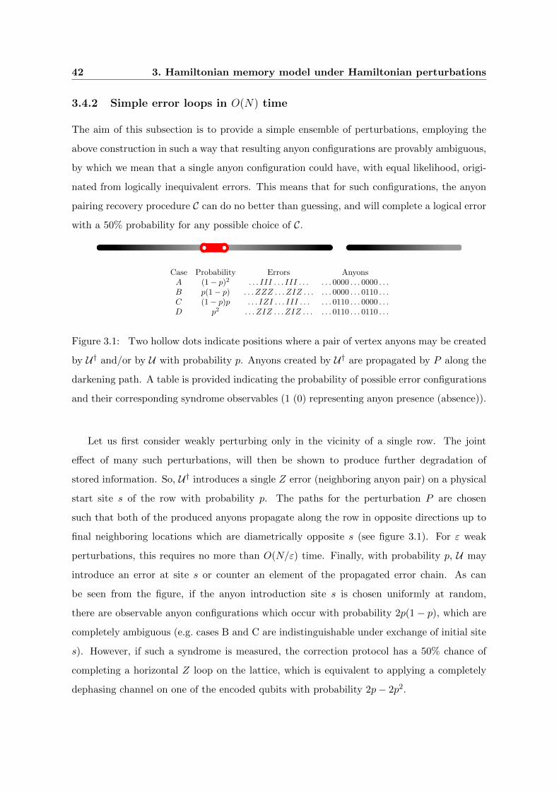
42 3. Hamiltonian memory model under Hamiltonian perturbations
3.4.2 Simple error loops in O(N) time
The aim of this subsection is to provide a simple ensemble of perturbations, employing the
above construction in such a way that resulting anyon configurations are provably ambiguous,
by which we mean that a single anyon configuration could have, with equal likelihood, origi-
nated from logically inequivalent errors. This means that for such configurations, the anyon
pairing recovery procedure C can do no better than guessing, and will complete a logical error
with a 50% probability for any possible choice of C.
Figure 3.1: Two hollow dots indicate positions where a pair of vertex anyons may be created
by U† and/or by U with probability p. Anyons created by U† are propagated by P along the
darkening path. A table is provided indicating the probability of possible error configurations
and their corresponding syndrome observables (1 (0) representing anyon presence (absence)).
Let us first consider weakly perturbing only in the vicinity of a single row. The joint
effect of many such perturbations, will then be shown to produce further degradation of
stored information. So, U† introduces a single Z error (neighboring anyon pair) on a physical
start site s of the row with probability p. The paths for the perturbation P are chosen
such that both of the produced anyons propagate along the row in opposite directions up to
final neighboring locations which are diametrically opposite s (see figure 3.1). For ε weak
perturbations, this requires no more than O(N/ε) time. Finally, with probability p, U may
introduce an error at site s or counter an element of the propagated error chain. As can
be seen from the figure, if the anyon introduction site s is chosen uniformly at random,
there are observable anyon configurations which occur with probability 2p(1− p), which are
completely ambiguous (e.g. cases B and C are indistinguishable under exchange of initial site
s). However, if such a syndrome is measured, the correction protocol has a 50% chance of
completing a horizontal Z loop on the lattice, which is equivalent to applying a completely
dephasing channel on one of the encoded qubits with probability 2p− 2p2.

3.4 Limitations of the 2D toric code 43
By applying such a perturbation family to i ≤ N rows of the lattice, the probability of
not having such a logically dephasing action take place becomes (1−2p+2p2)i, which may be
made arbitrarily small for large N (i.e. an odd number of horizontal Z loops is completed with
a probability exponentially close to 1/2). Completely analogous string like perturbations exist
for any of four logical operators defining the 2-qubit algebra associated to the ground space.
Again, by simultaneously considering such perturbations on a sufficiently large set of parallel
lines these operators too will be completed with a probability exponentially close to 1/2.
Furthermore, by allowing anyons to hop directly to next nearest neighbors (i.e. Eq. (3.33)), it
becomes possible to simultaneously introduce perpendicular yet commuting loop operations
as a result of anyon removal.
Simultaneously introducing the four logical operators independently with probability ex-
ponentially close to 12 , would yield a state exponentially close to a maximal mixture over the
code space. Our proof requires terms from different perturbation paths to commute, indi-
cating a possible obstacle to achieving this. In practice however, given that different anyons
follow roughly ballistic trajectories with a relatively small spread, this does not pose an issue.
In appendix 3.C, we show how it is possible to select the set of anyon trajectories in the per-
turbation such that the order of anyon crossing is well defined (exponentially well in N). In
turn, this implies an exponentially small deviation from the result of performing such anyon
propagations in order, resulting in a state exponentially close to a maximal mixture on the
four dimensional code-space.
Finally, it is worth mentioning that exactly the same perturbation construction may be
applied to the protecting Hamiltonian proposed by Chesi et al. [27] which presents long
range repulsive interactions among anyons. However, it must be made clear that the resulting
perturbation will, like the unperturbed Hamiltonian, also involve long range interactions. In
the case that has been studied numerically, which introduces a constant energy penalty for
every arbitrarily distant pair of anyons, our perturbation construction provides exactly the
same result for the information lifetime as for the original TC Hamiltonian.
3.4.3 Localization in 2D stabilizer codes
In the perturbations constructed to introduce logical errors in the toric code, there is a strong
use of the energy degeneracy of subspaces with the same number of anyons. The strengths

44 3. Hamiltonian memory model under Hamiltonian perturbations
of the different stabilizer terms in the 2D toric code manifest as strengths of local magnetic
fields in the effective Hamiltonian of the propagation [67]. However, having exactly the same
strength for all local Hamiltonian terms is not an essential feature of the 2D toric code or of
stabilizer Hamiltonians in general.
In the unperturbed picture of stabilizer Hamiltonians, excitations are completely localized.
However, when different excitations live in a degenerate energy space, perturbations may be
very effective at propagating them. In the spirit of Anderson localization, different stabilizer
term strengths may be randomly chosen from some range γupper > γlower > 0, with the hope
of protecting against anyon propagation terms.
However, for each such random instance, a specific Hamiltonian perturbation may “smooth”
this distribution to take on, at random, only a finite number of discrete energy values, sepa-
rated by ε, the strength of the perturbation. The number of such possible values is given by
dγupper−γlower
ε e, which is therefore also the average spacing between sites of the same energy.
Hence, by selecting propagation terms of a similar size, the hopping scheme can route around
the uneven energy landscape and introduce a logical error. Thus, the argument is unable to
guarantee protection against any constant sized perturbation. Nevertheless, it may be that
the perturbation terms necessary to break the code should involve a larger number of bodies,
which would definitely be an improvement.
In the case of the 2D toric code [67], and all other 2D local stabilizer Hamiltonians [22, 69],
there are always logical operations with string like support. This means that, albeit with
some possible energetic smoothening, the scheme presented in section 3.4.2 can be adapted to
introduce logical errors in arbitrary 2D stabilizer Hamiltonians, meaning that the asymptotic
lifetime which 2D N × N stabilizer codes may guarantee against weak local perturbations
cannot be more than O(N).
3.4.4 Logical errors in O(logN) time
In the previous section, we gave a rigorous upper bound of O(N) on the information lifetime
of the toric code. This bound coincides with the one provided by Kay in [67], which required
initial anyons in the system to be introduced by an unspecified environment. In this subsec-
tion, we provide an exponentially tighter bound by concentrating on specific choices for error
correction protocols. We argue that it is possible for a Hamiltonian perturbation to introduce

3.4 Limitations of the 2D toric code 45
4S+4
Figure 3.2: Anyon pairs corresponding to each thick red edge may be created by U†. After
a time tf , the right anyon from each pair introduced will be propagated a distance 4S + 2 to
the right introducing Z errors along the darkening paths. Finally, U acting on the same red
segment may move an unpropagated anyon one position to the right or create a neighboring
anyon pair on it. The number of big steps (or equivalently of crossings) during the upward
propagation is given by S, which in the case of the figure is 2.
ambiguous distributions of anyon configurations in a time logarithmic in N , i.e. after a time
tf ∼ O(logN), error correction succeeds with probability not much higher than 1/2. Figure
3.2 schematically presents one such perturbation, indicating where anyon pairs should be
introduced, and paths Pk along which they should propagate. The fact that the trajectories
have only simple crossings allows them to be implemented by weak local Hamiltonian per-
turbation terms involving at most 8 bodies, as obtained from Eq. (3.33), with p, q being next
nearest neighbors. Furthermore, the trajectory length is no more than twice the distance at
which the anyon pair is finally separated.
The length of anyon propagation trajectories is 8S + 4, where
S =
⌈lnN
2p
⌉, (3.39)
and each has 2S simple crossings with other trajectories. The time required to perform such
a propagation by fixed strength local perturbations is proportional to S (i.e. logarithmic in
N).
A relevant property of such a perturbation is that anyons observed when performing
unperturbed error correction after an evolution time tf are always collinear. The anyon type
and line direction may be chosen to coincide with any of the logical operations, translating
to the fact that any logical error may be introduced. This also has the desirable effect of
simplifying the analysis of anyon matching criteria. There are only two logically inequivalent
46 3. Hamiltonian memory model under Hamiltonian perturbations
anyon matchings on the line, which are the two perfect matchings in which each anyon is paired
with one of its two nearest neighbors (i.e. right or left). The point is that one matching will be
logically equivalent to the actual trajectories performed by the anyons, canceling any errors
introduced, whereas the other will complete the actual paths into a logical error. A simple
criterion to determine which case we are dealing with is to count how many times the actual
trajectories, together with the anyon matching, cross a vertical line or any homologically
equivalent curve. An odd number of crossings means that a logical error has been completed,
whereas an even number of crossings means that the proposed pairing has been successful at
error correcting.
We study the success probability of two apparently reasonable matching criteria. The first
minimizes the furthest distance among paired anyons. The second, for which a polynomial
algorithm is known [122], consists of minimizing the sum of distances among paired anyons.
Proofs and numerics will be provided for the large N regime given by N � 4S + 2 which
convey a high logical error rate.
Anyon matching that minimizes L∞
Let us first consider minimizing the furthest distance among paired anyons. This is the L∞
norm of the vector with components given by the individual distances among anyons paired
by the matching. We will prove that the probability of introducing a particular logical error
is close to 1/2 by considering two disjoint scenarios. The first is the very unlikely scenario in
which, on syndrome measurement, two consecutive anyons are measured at a distance ≥ D
(by consecutive, we mean no additional anyons were measured in the interval between them).
The second is composed of anyon distributions consistent with the measurement of a fixed
pair of consecutive anyons at a distance ≤ D. For such distributions, the number of activated
anyon paths passing completely over the fixed pair is shown to be odd with probability very
close to 1/2.
Let us first bound the probability of observing two consecutive anyons at a distance greater
than D in the syndrome measurement for the evolved state. Given a fixed region of length
D, at least bD/4c different potential anyon paths start and end in it. Furthermore, assuming
D < 4S, the probabilities for not measuring anyons in this region are independent and are
1− p for each end of an anyon path and (1− p)2 for each start of an anyon path, since both

3.4 Limitations of the 2D toric code 47
U and U† could have created anyons in this case. The anyon-free region can begin in any
of N locations of the full loop. Thus, regardless of correlations, the probability of having D
consecutive anyon-free sites is upper bounded by N(1− p)3bD/4c.
Assume now that a pair of consecutive anyons is measured at a distance no greater than
D. There are at least b(4S − D)/4c potential anyon paths going over this region, each
with independent probability p of being observed. On syndrome read-out, the number of
such paths that is activated is odd with a probability approaching 1/2 at least as fast as
12(1± (1− 2p)b(4S−D)/4c). Since the L∞ norm correction completes a logical error if the most
distant consecutive anyon pair is covered by an odd number of activated anyon paths, then
by inserting S = d ln(N)2p e and D = d8 ln(N)
5p e, we get a probability lower bound for logical errors
which approaches 1/2 as 1/2(1−N−1/5).
Anyon matching that minimizes L1
Let us now consider the anyon pairing criterion that minimizes the total sum of distances
among paired anyons. Since all anyons are found on a loop of length N , this criterion will
always choose a pairing with total distance no greater than N/2. Thus it will successfully
error correct if and only if the total distance of regions of the loop covered an odd number
of times by observed anyons is no greater than N/2. By taking S to be d lnN2p e, we expect to
find roughly half of the sites flipped. To see this, note that, on average, each site is covered
approximately Sε times. Moreover, the probability of each site being covered an odd number
of times is 12 [1− (1−2p)S ]. For small p and the chosen value of S, the average number of sites
covered an odd number of times is approximated by N2 − 1
2N . Furthermore, we expect the
actual number of such sites to approximately follow a normal distribution around this value,
which would imply that logical errors are completed with a probability close to 12 . However,
since the flipping of different nearby sites are highly correlated events, it is not clear how to
go about proving this. Instead, computer simulations (Fig. 3.3) provide very strong numerical
evidence.
3.4.5 Discussion
We have proven that Hamiltonian perturbations can completely destroy the information stored
in the 2D toric code in a time proportional to N . The only assumptions are that the precise
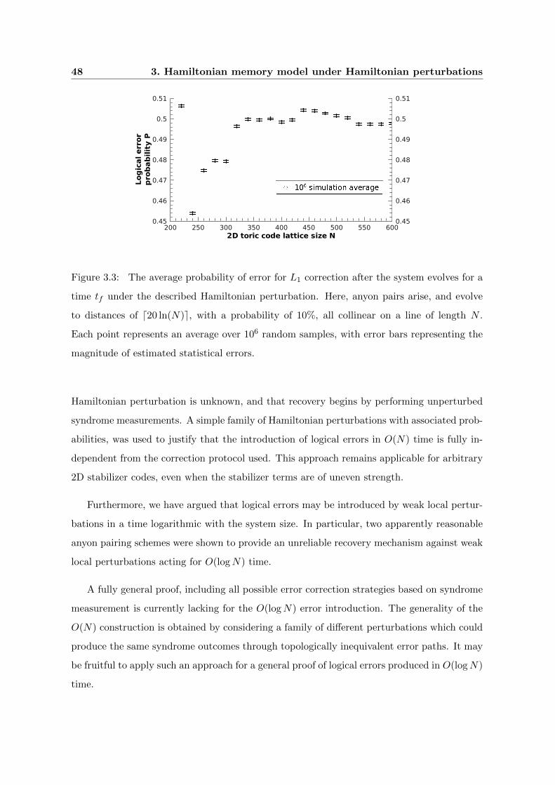
48 3. Hamiltonian memory model under Hamiltonian perturbations
Logical
error
probab
ility P
0.450.460.470.480.490.5
0.51
0.450.460.470.480.490.50.51
2D toric code lattice size N200 250 300 350 400 450 500 550 600
Figure 3.3: The average probability of error for L1 correction after the system evolves for a
time tf under the described Hamiltonian perturbation. Here, anyon pairs arise, and evolve
to distances of d20 ln(N)e, with a probability of 10%, all collinear on a line of length N .
Each point represents an average over 106 random samples, with error bars representing the
magnitude of estimated statistical errors.
Hamiltonian perturbation is unknown, and that recovery begins by performing unperturbed
syndrome measurements. A simple family of Hamiltonian perturbations with associated prob-
abilities, was used to justify that the introduction of logical errors in O(N) time is fully in-
dependent from the correction protocol used. This approach remains applicable for arbitrary
2D stabilizer codes, even when the stabilizer terms are of uneven strength.
Furthermore, we have argued that logical errors may be introduced by weak local pertur-
bations in a time logarithmic with the system size. In particular, two apparently reasonable
anyon pairing schemes were shown to provide an unreliable recovery mechanism against weak
local perturbations acting for O(logN) time.
A fully general proof, including all possible error correction strategies based on syndrome
measurement is currently lacking for the O(logN) error introduction. The generality of the
O(N) construction is obtained by considering a family of different perturbations which could
produce the same syndrome outcomes through topologically inequivalent error paths. It may
be fruitful to apply such an approach for a general proof of logical errors produced in O(logN)
time.

3.5 Limitations of the 2D Ising model 49
3.5 Limitations of the 2D Ising model
In present day classical computers, magnetic domains are widely used to provide passive
safekeeping of classical information. The Ising model is usually used to elucidate the origin of
such long lived magnetized states as a collective effect arising from microscopic local 2-body
interactions
HIsing = −J∑〈i,j〉
ZiZj . (3.40)
In two and higher spatial dimensions, the nearest neighbor Ising model presents a finite
temperature phase transition between a disordered phase and an ordered magnetized phase.
However, it has long been known that such a system looses its asymptotic bistability under
the bias produced by even the weakest of magnetic fields [106, 30, 51]
HIsing = −J∑〈i,j〉
ZiZj + ε∑j
Zj . (3.41)
Such studies consider the dynamics of minority droplets in a 2D Ising model as given by
phenomenological equations or the Metropolis algorithm. For a Metropolis algorithm in
which such a systematic magnetic field ε is included, there is only one stable phase parallel
to the field. The anti-parallel phase becomes metastable, with a lifetime exponential in J/ε.
Dependence of the information lifetime on lattice size N appears only for the small N ≤ 4J/ε
and will thus not appear if one first takes the limit for large N .
In this section we consider storing one bit of classical information subject to a quantum
evolution of a perturbed 2D Ising Hamiltonian. The observable on which the classical bit is
encoded is assumed to be the overall direction for magnetization Z = majjZj . The pertur-
bations may conceptually be split into two parts, Z parallel magnetic fields which introduce
additional degeneracies to the Hamiltonian, and transverse magnetic fields or many body
terms which couple the new ground states, introducing a hopping between them. The pertur-
bation terms considered will not show support or intensity growing with N , and they will be
capable of introducing logical errors to the unperturbed logical observable Z in a time also
independent of N .

50 3. Hamiltonian memory model under Hamiltonian perturbations
3.5.1 Hamiltonian perturbation proposal
Consider dividing the N × N 2D periodic lattice with a chessboard pattern of squares of
M×M spins where M > 4J/εmax and J is, again, the nearest neighbor Ising coupling constant
and εmax is the greatest local perturbation strength one expects the Hamiltonian to protect
information against. For simplicity, we assume N = 2nM , where n is an integer. Consider
alternately introducing ±εZj magnetic fields in the lattice site j belonging to white/black
squares of the chessboard pattern respectively. The value ε is chosen homogeneously for
each square such that the energy difference, 2εM2, from fully field parallel and anti-parallel
configurations of each square exactly matches the maximum energy difference for border Ising
terms 8MJ . For N � J/ε such a perturbation is always possible.
The point is that now, the ground space of the system acquires a much higher degeneracy,
i.e. between 22n2+1 − 1 and 24n2. Each black square could be fully magnetized parallel to
its preferred field direction or parallel to the direction of its four neighboring squares if it is
opposite. By taking one spin variable for each square, the ground states may be identified
with those of a 2D n × n anti-ferromagnetic Ising model with magnetic field. Three impor-
tant ground states are the two fully magnetized lattice configurations and the checkerboard
configuration in which all spins are fully aligned to their local magnetic field. The gap of
these ground states with respect to low lying exited states is 2ε, which is the energy penalty
of flipping a corner lattice site of a square that is fully oriented in the direction of the field
but anti-parallel to the two neighboring squares adjacent to the stated corner.
A flipping term for each square of the chessboard should be of the form α⊗
j Xj , where
the j is taken over all the M2 sites in the square. Such terms can be introduced either on
all black squares or all white squares. This would respectively couple one of the two fully
magnetized configurations with the checkerboard configuration, achieving a full swap of state
in a time tflip = πα . This evolution is exact when such M2-body terms of norm α are allowed,
which implies that a proof of Hamiltonian stability will not only require assuming sufficiently
weak perturbation terms but also a specific bound for the number of bodies on which such
terms act.
Let us now focus on the magnitude of α. This is the coefficient for a many body term, in
which the size of the support scales like M2 = (4J/ε)2, independent of N . One may consider
obtaining such a term from theM2-th order degenerate perturbation theory expansion of fields
3.5 Limitations of the 2D Ising model 51
of the form ε2∑
j Xj . For perturbation theory to be strictly valid, one needs M2ε2 < ε. Even
then, this small magnitude must be taken to the M2-th power to obtain the first non vanishing
expansion term. The time required to flip all spins in a plaquette is then proportional to:
α ≈ ε2
(ε2
ε
)M2
≈ εM−2(M2−1) = ε( ε
4J
) 32J2
ε2+2. (3.42)
This expression has no dependence on N and the same perturbation can be introduced in all
squares of a given color to yield a fixed flip time. Furthermore, we note that the state of those
chessboard squares which are not perturbed is fixed and may be traced out exactly. Hence,
the second set of perturbations applied are fully independent and degenerate perturbation
theory may be rigorously applied.
3.5.2 Discussion
Although the flip time shows no dependence on N , it grows faster than exponentially in
terms of 4J/ε. It may well be that for magnetic domains, describable by such a 2D Ising
Hamiltonian as Eq. (3.40), the ratio 4J/ε is sufficiently large to provide a lifetime longer than
would be experimentally verifiable. More importatntly, we are dealing with an extremely
simplified model, with the particularity of neglecting any long range interactions of actual
physical systems and more importantly, dissipative terms in the form of decoherence which
would dissallow the coherent evolution and thus help in preserving the classical information.
The fact that the perturbation is unknown means that if such a checkerboard state is
observed on read-out, information is not recoverable. Such schemes may clearly be generalized
to higher dimensions and to deformations of the checkerboard pattern. The existence of such
perturbations elucidates important limitations for statements one may formally prove about
the classical memory reliability of the Ising model, and therefore what conclusions one might
draw about the presence of a macroscopic energy barrier (string tension) which the 2D Ising
model certainly possesses. However, it is not clear that these arguments can be applied, for
instance, to the 4D toric code since it is a feature of classical memories, but not quantum
ones, that local fields can split degeneracies.
52 3. Hamiltonian memory model under Hamiltonian perturbations
3.6 Aggressive noise models
In previous sections, we explored the effects of Hamiltonian perturbations on quantum mem-
ories, and particularly on the 2D toric code. We also considered examples of local cold
environments perturbatively coupled to a system, as illustrated by Secs. 3.2.2 and 3.3. The
only energy available in these scenarios was due to local perturbations on the system plus
environment. Intuitively, a small but constant energy density proportional to ε was allowed.
While this energy is potentially O(Nd) for a d spatial dimension lattice of Nd qubits, it is
difficult to concentrate it in specific regions in order to generate logical errors. In compari-
son, stabilizer codes only require O(Nd−1) energy to implement a logical gate through local
rotations.
More aggressive noise models may locally introduce large amounts of energy into the
system while keeping perturbation magnitudes weak. Such an example is provided by weak yet
time dependent Hamiltonian perturbations. These are relevant when one considers effective
protecting Hamiltonians in the interaction picture [23]. Another possibility is to consider the
weak coupling of the system to an environment which starts in a high energy state. Noise
constructions for these models shall be presented in this section.
In calling such noise models aggressive, we convey the fact that we do not expect “rea-
sonable” Hamiltonian protection schemes to guarantee a long lifetime against such models.
Thus, their study may help identify required restrictions on the noise model in order to allow
for provably robust Hamiltonian protected memory models. Furthermore, it may provide
insight regarding potentially fruitful proof techniques.
3.6.1 Time-varying Perturbations
When considering Hamiltonian perturbations, we assumed that we were unable to determine
the new ground space due to the perturbation, and thus encoded in the original ground state
space. One might consider an intermediate setting where encoding can be achieved in the
perturbed code-space, perhaps due to an adiabatic evolution such as proposed by [54], or by
a precise characterization and compensation of the perturbations present at the start of the
storage time. However, in real experiments, stray fields responsible for perturbations may
fluctuate in time. Again, if one can track adiabatic changes in the perturbations, the proof of
Hastings and Wen [57] continues to hold because Lieb-Robinson bounds apply to time-varying
3.6 Aggressive noise models 53
local Hamiltonians, and we can therefore adapt the final error correction step as well. Instead,
we proceed assuming it is impossible to precisely learn this time variation.
Adiabatically varying perturbations
One extreme case to consider is that the perturbation varies adiabatically, so that the system
remains in its ground state space. If we do not apply error correction, then we are concerned
with how long it takes before the initial and final ground states have a small overlap. We
shall assume that the original Hamiltonian H of N qubits has an energy gap γ, and we will
consider the time-varying perturbation
V = U(t)HU†(t)−H
where, as before,
U(t) =
N∏j=1
e−itεXj/T
and T is the total time of the evolution, i.e. small local rotations are gradually introduced.
At any time 0 ≤ t ≤ T , the effective Hamiltonian U(t)HU†(t) has the same energy gap as
H, which means that the adiabatic condition is satisfied for T ∼ 1/poly(γ). From previous
considerations, Eqn. (3.61), we know that the overlap of the initial state |ψ(0)〉 and the evolved
state, the ground state of the adiabatically perturbed Hamiltonian, have an average overlap
of no more than tr (P0) (1 − 34 sin2(tε/T ))N . For large N and small ε, this means that the
final overlap is of the order tr (P0) exp(−3ε2N4 ) if a phase of error correction is not involved.
When error correction is introduced to this scenario, this maps into the situation where
our quantum memory is initially encoded in the perturbed subspace, but decoding is using the
original, unperturbed, error correction strategy. In the specific instance of the perturbation
U(T ), we find that X rotations are applied probabilistically on each site, and hence our QECC
must have a superior error threshold.
Hastings and Wen [57] reveal a similar interpretation holds for all possible perturbations
since all local terms are converted into quasi-local rotations.
Rapidly oscillating perturbations
Another extreme scenario is when perturbations are allowed to oscillate with arbitrary fre-
quencies. A simple construction shows that for stabilizer Hamiltonians, this allows the in-

54 3. Hamiltonian memory model under Hamiltonian perturbations
troduction of arbitrary errors in constant time. We expect that optimal control theory may
provide the tools to generalize such results to arbitrary Hamiltonians.
Consider a stabilizer HamiltonianH0 and a logical error to implement L = PMPM−1 . . . P2P1,
which is decomposed into Pauli operators Pi on different sites. We then consider the time
dependent Hamiltonian perturbation
V (t) = ε(t)∑i
e−iH0tPieiH0t. (3.43)
This perturbation is weak if ε(t) is sufficiently small. Furthermore, given that H0 is a stabilizer
Hamiltonian, V (t) may be written as a sum of local terms (at least as local as the stabilizer
operators). Finally, the dependence of ε(t) on time, is to allow for ε(0) = 0 which makes the
initial encoding equivalent for both perturbed and unperturbed Hamiltonians.
The point of such a perturbation, is that it is possible to explicitly calculate the evolution
of the system state in the interaction picture.
|ψI(t)〉 = Πie−iPi
∫ t0 ε(t
′)dt′ |ψI(0)〉 (3.44)
This means that after a constant time tf such that π2 =
∫ tf0 ε(t′)dt′, the target operation L
is perfectly implemented in the interaction picture. If |ψ(0)〉 is an eigenstate, then L is also
implemented in the Schrodinger picture, modulo a global phase.
Taking L to be a logical operator of the stabilizer code used, this means that time depen-
dent perturbations of sufficiently high frequency can destroy stored information in constant
time. Here, sufficiently high frequency refers to having perturbation terms which oscillate
with frequencies at least as high as those corresponding to localized excitations.
3.6.2 Stabilizer Hamiltonians and energetic environment
In what follows, we consider a model in which an environment starts out in an arbitrarily
energetic state. However, the couplings between system and environment are required to
remain small and local.
For simplicity, we assume that the system is defined by a stabilizer Hamiltonian HS and
that it starts out in an eigenstate |ψ0〉 of all stabilizer operators. We will consider a sequence
of M Pauli operators on different sites L = PMPM−1 . . . P2P1 compounding to a logical
operation. In the case of translationally invariant stabilizer codes, explicit constructions
3.6 Aggressive noise models 55
for these operators are given in [69]. Finally, we may assume a code state |ψ0〉, such that
〈ψ0|L |ψ0〉 = 0.
Motivated by the realization that, in order to introduce logical errors, we need to transfer
some energy from the environment to the system, we choose a specific environment Hamilto-
nian HE = −H∗S (at this point, the complex conjugate is unnecessary, but will become useful
later). This means that all steps up in energy in the system correspond to an identical step
down in energy in the environment. We start the environment state in |ψ∗0〉.In this scenario, the coupling
HSE = ε
M∑i=1
PS,i ⊗ P ∗E,i (3.45)
is enough to produce the logical error L in constant time π2ε . To see this, consider the two
states PS,i |ψ0〉P ∗E,i |ψ∗0〉 and PS,iPS,i |ψ0〉P ∗E,iP ∗E,i |ψ∗0〉. Here, the subindex i is an arbitrary
binary vector indicating which values of j a product of PS,j (respectively P ∗E,j) should be taken
over. First of all, since we have assumed HS is a stabilizer, and the PS,i are Pauli operators,
the aforementioned states are zero eigenstates of HS ⊗ 11E + 11S ⊗ HE . Furthermore, the
effective Hamiltonian for the perturbation term εPS,i ⊗ P ∗E,i acting on the pair of states
PS,i |ψ0〉P ∗E,i |ψ∗0〉 and PS,iPS,i |ψ0〉P ∗E,iP ∗E,i |ψ∗0〉 is just a matrix
ε
0 1
1 0
,
independent of i. This means that we can consider the action of the different PS,i⊗P ∗E,i terms
independently:
e−iHSEt |ψ0〉 =
(M⊗i=1
e−iεPS,i⊗P∗E,it
)|ψ0〉 .
Due to the effective Hamiltonian, PS,i |ψ0〉P ∗E,i |ψ∗0〉 is mapped to PS,iPS,i |ψ0〉P ∗E,iP ∗E,i |ψ∗0〉 in
a time π/(2ε). Thus, the effect of the entire perturbation is to rotate, in a time π/(2ε) from
|ψ0〉 to L |ψ0〉.Of course, this approach requires the environment state to have a very high initial energy,
namely to start in one of its highest energy states. A refinement of this argument allows us
to only change the sign of stabilizers in HE which share support with L. For a local stabilizer
code in d spatial dimensions consisting of Nd qubits, it was shown [69, 22] that there are
logical operators L with support on k ∝ Nd−1 sites. The initial state of the environment
56 3. Hamiltonian memory model under Hamiltonian perturbations
|ψE〉 = |ψ∗0〉 is still an eigenvector of these stabilizers, with the same eigenvalues. Thus,
coupling to an environment with an energy proportional to Nd−1, may also introduce logical
errors in the same time. This means that the energy required from the environment per
system qubit tends to 0 as 1N (compare to perturbations, which introduce an energy ε per
site). The catch however, is that the distribution of the energy in the initial environment is
highly specific and is in general very different from distributions that may be provided by low
temperature thermal states.
We conclude that no stabilizer Hamiltonian will be capable of providing a guarantee for the
logical integrity of stored information under the presence of an adversarial, weakly coupled,
local environment. Further statistical assumptions such as energy distribution associated to a
low temperature environment state need to be included in addition to the weak local coupling
assumptions.
3.6.3 Non-stabilizer Hamiltonians
Stabilizer Hamiltonians are not the only possible candidates for providing information pro-
tection, although they are particularly attractive because local errors remain as local errors
(not propagating or multiplying in the absence of perturbations). Let us now consider the
more general case of distance preserving Hamiltonians i.e. ones which might not leave local
errors perfectly localized, but do not increase the distance of the error as defined by an error
correcting code4. Using the same construction as in the previous section, we will show that
weak coupling to an environment can also introduce the relevant logical error into a distance
preserving Hamiltonian (i.e. a logical operation converting between the most distant code
states) for classical memories, by which we mean that one set of local errors becomes irrel-
evant, say Z errors, and the presence of a logical error on the classical bit depends only on
the local X errors present. The distance preserving assumption means that the number of X
errors is preserved, [HS ,∑
i Zi] = 0. The maximum distance between any 2 states is for the
eigenstates⊗
i |0〉i and⊗
i |1〉i, suggesting we should use these states for encoding.
Similarly to the previous subsection, we introduce an environment, and a perturbative
4As an aside, note that the 3D XZ-compass code [11] is an example of a code where the errors do not
remain in fixed positions, but preserve the values of the observables (since the observables commute with the
Hamiltonian). This suggests that applying explicit error correction is already likely to become much more
problematic for these codes.
3.6 Aggressive noise models 57
coupling between system and environment,
H(ε) = HS ⊗ 11E + 11S ⊗HE + ε∑i
Xi,S ⊗Xi,E . (3.46)
The system Hamiltonian is weakly coupled to a “mirror” system HE = −H∗S . This pertur-
bative coupling is responsible for the evolution of a mirrored state |0〉⊗N |0〉⊗N , eigenstate of
the unperturbed Hamiltonian H(0).
To analyze the evolution, let us consider the action of the operators Xi in terms of the
eigenstates of HS . Due to the commutation relation, there must be(Nm
)eigenstates {|ψm,j〉}
of HS which are simultaneous eigenvectors of∑
i Zi with eigenvalue 2m − N . We can thus
express the eigenvectors |ψm,j〉 of HS in terms of the canonical basis as
|ψm,j〉 =∑
i:w(i)=m
α(m)i,jXi |0〉⊗N =∑
i:w(i)=m
α(m)i,j |i〉 , (3.47)
where i are binary vectors with m non zero components and |i〉 are the respective states from
the canonical basis. The matrix α(m) is unitary as it relates two orthonormal bases of the
same subspace. Define
|m〉 =1√(Nm
) ∑i:w(i)=m
|i〉 |i〉
=1√(Nm
) ∑j,k,(i):w(i)=m
α(m)∗i,jα(m)i,k |ψm,j〉∣∣ψ∗m,k⟩
=1√(Nm
)∑j
|ψm,j〉∣∣ψ∗m,j⟩ . (3.48)
From this, one obtains that
(HS ⊗ 11E − 11S ⊗H∗S) |m〉 = 0, (3.49)
implying that any non trivial evolution of |m〉 arises exclusively from the perturbative coupling
and is given by
H(ε) |m〉 = εJm∣∣m− 1
⟩+ εJm+1
∣∣m+ 1⟩, (3.50)
with Jm =√m(N + 1−m). These are precisely the coefficients performing perfect state
transfer between∣∣0⟩ = |0〉⊗2N and
∣∣N⟩ = |1〉⊗2N in a constant time t = π2ε [29, 68].
These results exclude the possibility of proving robustness against weak adversarial cou-
pling to an arbitrarily initialized environment, even of many classical memories using the

58 3. Hamiltonian memory model under Hamiltonian perturbations
repetition code (such as Ising models). We learn that if the environment can provide enough
energy, then even weak local couplings may be sufficient to produce logical operations. This
also motivates the desire to encode in the ground state space of the Hamiltonian since, were
we to encode in a higher energy subspace, the environment needs less energy to cause de-
structive effects. Alternatively, the mechanism presented here could present a useful way to
implement gates on a memory.
3.7 Further applications
Constructed perturbations and results presented in this chapter have focused on elucidating
limitations of passive quantum memories. However, our results may be recast in the following
other scenarios.
Adiabatic Quantum Computation- The standard approach to adiabatic quantum
computation consists of implementing an adiabatic evolution
H(t) = f(t)Hi + (1− f(t))Hf , (3.51)
between Hamiltonians Hi and Hf , where f(0) = 1 and f(T ) = 0. While the ground state of
the initial Hamiltonian Hi is expected to be readily prepared, the ground state of the final
Hamiltonian Hf encodes the result of the desired quantum computation. An energy gap no
less than γ between ground state and excited states of H(t) is required for the duration of
the adiabatic evolution.
In this context, it is possible that Hamiltonian perturbations could change the initial or
final ground state, and maybe even close the gap during the Hamiltonian trajectory. For
example, a time dependent perturbation
V (t) = UH(t)U† −H(t), (3.52)
with U defined as in Eq. (3.3), can make the perturbed initial and final ground states almost
orthogonal to the unperturbed versions (see Eq. (3.8)), while keeping the same gap as H(t).
Even assuming the perturbed initial ground state is exactly prepared, only if the final state
belongs to a code space with an error threshold, will it be possible to reliably recover the
desired result, as in 3.6.1.
3.8 Conclusions 59
Connections between adiabatic quantum computation and passive quantum memories
can be expected to continue into the regime where error correction is incorporated, and
future studies may better elucidate the issues involved in developing a fault-tolerant theory
of adiabatic quantum computation [82].
Topological Quantum Computation- Difficulties in implementing quantum memories
can also be related to some of the difficulties in implementing a topological quantum compu-
tation. In particular, in section 3.4 we illustrated how constant Hamiltonian perturbations
can create and propagate anyons in the 2D toric code. In the context of topological quantum
computation, where gates are implemented through the braiding of anyons, the existence of
perturbations capable of creating and propagating anyon pairs is at least equally disturbing
as in the memory scenario.
Quantum Simulations- One of the most interesting uses of a quantum computer is likely
to be the simulation of other quantum systems. While one could express these simulations
in terms of the circuit model of quantum computation, and from there create a circuit-based
theory of fault-tolerance for quantum simulation, it would be advantageous to understand
how this could be implemented more directly, via the simulation of an encoded Hamiltonian.
A logical first step would be to encode the state of each subsystem to be simulated into
a quantum memory. Thus, establishing when quantum memories exist, or when they fail,
has implications in this case. One of the most commonly applied techniques in Hamilto-
nian simulation is that of the Trotter-Suzuki decomposition, where pulses of non-commuting
Hamiltonians are combined into one effective Hamiltonian to some accuracy δ. This inaccu-
racy may be treated as a time dependent Hamiltonian perturbation. Given the power such
perturbations were shown to have, it is with great care that one should consider the use of
passive quantum memories as elements for such quantum simulators.
3.8 Conclusions
In this chapter, we have studied several constraints on the extent to which a many body Hamil-
tonian can be expected to protect quantum information against weak local coupling to an
environment. First of all, we showed that gapped local Hamiltonians have eigenstates which
are asymptotically unstable under local Hamiltonian perturbations. This result, commonly
referred to as Anderson’s orthogonality catastrophe [10] shows that a gap is not sufficient to
60 3. Hamiltonian memory model under Hamiltonian perturbations
guarantee protection against errors [65, 53]. We proved that a weakly coupled cold environ-
ment can alter the evolution of any quantum state leading to an exponentially small overlap
between initial and final states in constant time. Taking these results together, we conclude
that quantum memory schemes must encode information into a logical subsystem instead of
restricting to a particular subspace.
When applied to the 3D XZ-compass model [11], a self-correcting quantum memory pro-
posal, we find that the standard QECC protocol is not capable of recovering the encoded
information after a constant time. This means that the unperturbed order parameter is not
preserved. Our results extend to other systems revealing that the code and error correct-
ing process must possess an error threshold. Similar conclusions may be drawn in scenarios
where information encoding and evolution follow a perturbed Hamiltonian but read-out and
decoding do not.
Further explicit local Hamiltonian perturbation constructions illustrate that while adapt-
ing for known perturbations is theoretically possible, arbitrary unknown perturbations can
destroy the storage properties of codes such as the 2D Toric code in a time O(logN). In
this case, the proposed adversarial Hamiltonian perturbation heavily relies on the absence
of a macroscopic energy barrier (it is possible to transform orthogonal encoded states via a
sequence of local operations while keeping intermediate states in a low energy subspace). By
considering the 2D Ising model, we have argued that, in and of itself, a macroscopic energy
barrier is not sufficient to protect against perturbations. Let us stress once more, that the
perturbations considered are highly atypical, and that furthermore, we expect that genuine
dissipation mechanisms will play a key role in analyzing the robustness of such models.
Finally, we have considered strong noise models such as time varying Hamiltonian per-
turbations and weak coupling to an arbitrarily initialized environment. We showed that
these noise models could apply logical transformations on information protected by stabilizer
Hamiltonians or distance preserving classical memories in constant time. Although we con-
sider such noise models to be too strong to be of practical relevance, we expect these result
to provide insight into how one may prove properties of passive quantum memories and un-
der which assumptions. For instance, since such time-varying Hamiltonian perturbations can
destroy the 4D toric code, then when trying to prove robustness against static perturbations,
Lieb-Robinson bounds are unlikely to be beneficial.
3.A State evolution in perturbed gapped Hamiltonians 61
Having proven a variety of limitations for quantum memory models and elucidated some
required conditions, the next step is to incorporate this deeper understanding into new de-
signs for quantum memories. One major route is to establish a set of necessary and sufficient
conditions under which a quantum memory is protected against unknown weak static per-
turbations. Under such a model, we may once again raise the question of whether good
protecting Hamiltonians in two or three spatial dimensions exist. Furthermore, one would
hope to find similar conditions under an extended perturbation model allowing a perturba-
tively coupled local environment. Here, a central problem is to determine which physically
realistic assumption may be made on the environment such that positive results are still at-
tainable (i.e. conditions on the initial state of the environment, such as it being prepared in
its ground state). Finally, one may study the possibility of engineering an out of equilibrium
environment to provide additional protection to quantum information.
3.A State evolution in perturbed gapped Hamiltonians
Energy gaps are considered as a positive feature for a protecting Hamiltonian, since they are
expected to provide an energetic barrier which an error process is required to overcome. How-
ever, it will be shown that for sufficiently large N , the fidelity of the unperturbed eigenstates
acquires an upper bound close to 1/2 after being evolved under the effect of a perturbed
Hamiltonian for a time inversely proportional to the gap energy γ.
If a system is perturbed, but we do not know the nature of the perturbation, the best
strategy is, arguably, to continue using the unperturbed encoding (i.e. the eigenstates of the
unperturbed Hamiltonian). The survival probability for an unperturbed eigenstate |ψ0〉 of H
after evolution under a perturbed Hamiltonian H for a given time t (Eq. (3.3)) is, without
error correction
S(t) =∣∣∣〈ψ0| e−itH |ψ0〉
∣∣∣2 =∣∣∣〈ψ0| Ue−itHU† |ψ0〉
∣∣∣2 , (3.53)
i.e. we can express S(t) as the overlap of U† |ψ0〉 with itself under the evolution of the
unperturbed Hamiltonian H. Furthermore, in terms of the eigenstate decomposition
U† |ψ0〉 =∑j
αj |ψj〉 where H |ψj〉 = Ej |ψj〉 , (3.54)
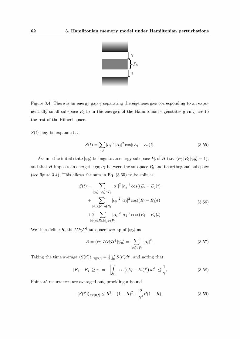
62 3. Hamiltonian memory model under Hamiltonian perturbations
Figure 3.4: There is an energy gap γ separating the eigenenergies corresponding to an expo-
nentially small subspace P0 from the energies of the Hamiltonian eigenstates giving rise to
the rest of the Hilbert space.
S(t) may be expanded as
S(t) =∑i,j
|αi|2 |αj |2 cos[(Ei − Ej)t]. (3.55)
Assume the initial state |ψ0〉 belongs to an energy subspace P0 of H (i.e. 〈ψ0|P0 |ψ0〉 = 1),
and that H imposes an energetic gap γ between the subspace P0 and its orthogonal subspace
(see figure 3.4). This allows the sum in Eq. (3.55) to be split as
S(t) =∑
|ψi〉,|ψj〉∈P0
|αi|2 |αj |2 cos((Ei − Ej)t)
+∑
|ψi〉,|ψj〉6∈P0
|αi|2 |αj |2 cos((Ei − Ej)t)
+ 2∑
|ψi〉∈P0,|ψj〉6∈P0
|αi|2 |αj |2 cos((Ei − Ej)t)
(3.56)
We then define R, the UP0U† subspace overlap of |ψ0〉 as
R = 〈ψ0| UP0U† |ψ0〉 =∑|ψi〉∈P0
|αi|2 . (3.57)
Taking the time average 〈S(t′)〉t′∈[0,t] = 1t
∫ t0 S(t′)dt′, and noting that
|Ei − Ej | ≥ γ ⇒∣∣∣∣∫ t
0cos((Ei − Ej)t′
)dt′∣∣∣∣ ≤ 1
γ, (3.58)
Poincare recurrences are averaged out, providing a bound
〈S(t′)〉t′∈[0,t] ≤ R2 + (1−R)2 +2
γtR(1−R). (3.59)

3.B The toric code 63
Although the bound in Eq. (3.59) is minimized for R = 1/2, this does not imply that the
smallest values for 〈S(t′)〉t′∈[0,t] are actually obtained for R = 1/2.
A sufficient condition for the existence of a weak perturbation yielding R = 12 may now
be obtained by means of continuity arguments. First, note that R depends continuously on
the parameter ε appearing in the definition of the rotation U , and R = 1 for ε = 0. This
means that if, for some ε0 > 0, we find that R < 1/2, then R must be equal to 1/2 for some
smaller positive value 0 < ε < ε0.
As in the previous subsection, we may take 〈R〉U as an average of the overlap R over
different directions of the rotation U . An expression for 〈R〉U , in terms of the depolarizing
channel is given by
〈R〉U = tr(P0∆⊗Nλ(ε) (|ψi〉 〈ψi|)
). (3.60)
Including the dimension of the subspace P0, the same bound as in Eq. (3.8) may be used,
leading to
〈R〉U ≤ tr (P0)
(1− 3
4sin2(ε)
)N. (3.61)
If the asymptotic growth of tr (P0) is slower than(1− 3
4 sin2(ε))−N
, the bound (3.61) will
be exponentially decreasing with N . This means that for sufficiently large N , and for most
directions of rotation, there is some small rotation parameter ε yielding R = 1/2. For the
important case of small ε and a constant dimension tr (P0), large N refers to N ∼ O(ε−2).
For those U leading to R = 12 , the time averaged survival probability 〈S(t′)〉t′∈[0,t] for the
corresponding perturbation may be bounded as
〈S(t′)〉t′∈[0,t] ≤1
2+
1
2γt. (3.62)
We thus obtain that the overlap of initial encoded states and uncorrected evolved states will
drop to values not much larger than 12 in a time inversely proportional to the gap γ.
3.B The toric code
Kitaev introduced the toric code [74] with the intention of achieving reliable storage of quan-
tum information at the physical level, as in classical stable storage, rather than by periodi-
cally performing explicit error correction procedures. He proposed that the Hamiltonian of
the physical system being used to store the quantum information could, by its nature, make

64 3. Hamiltonian memory model under Hamiltonian perturbations
the information stable. His proposal consisted of a 2D system with non trivial topology (such
as the surface of a torus) with a stabilizer Hamiltonian composed of local terms. Qubits could
then be stored in the ground subspace with a degeneracy of 4g, with g being the genus of the
surface on which the physical qubits are located.
In the toric code Hamiltonian, the physical qubits are located on the edges of a planar
grid covering the 2D surface. For concreteness and simplicity, we shall restrict to the case
were the surface is a torus and the grid is an N ×N square lattice (i.e. 2N2 physical qubits).
The Hamiltonian is composed of commuting terms which are products of Pauli operators on
different sites (it is a stabilizer Hamiltonian). For each vertex s of the grid, there is a star
(or vertex) term As =∏j∈star(s)Xj which is the product of X operators over all the qubits
of edges reaching s. Analogously, for each face p of the grid, there is a plaquette (or face)
term Bp =∏j∈boundary(p) Zj which is the product of Z operators over all the qubits of edges
surrounding the face p. Since each vertex and face have either 0 or 2 common edges, the
terms As and Bp always commute. Hence all terms of the toric code Hamiltonian
H = −∑s
As −∑p
Bp (3.63)
commute, and may be simultaneously diagonalized. Since∏sAs = I and
∏pBp = I, there
are only 2N2 − 2 independent binary quantum numbers asociated to these terms (stabilizer
operators) and each valid configuration determines a subspace of dimension 4. Due to this,
violations of plaquette (vertex) conditions As |ψ〉 = |ψ〉 (Bp |ψ〉 = |ψ〉) always come in respec-
tive pairs. Following usual nomenclature, virtual particles called vertex (plaquette) anyons
are respectively associated to these excitations. The set of stabilizers may be completed
with a pair of logical observables consisting of the product of Z (X) operators along non
contractible loops on the lattice (dual lattice), which may not be expressed as a product
of plaquette (star) terms as illustrated in figure 3.5. Together with the set of Hamiltonian
stabilizers any commuting pair of these four logical operators (X1, X2, Z1 and Z2) uniquely
determine the state.
A stated prerequisite for using the toric code as a protecting Hamiltonian is that the
energy splitting of the ground space due to Hamiltonian perturbations should be small. This
is argued through the use of degenerate perturbation theory and the fact that it only gives
non-zero splitting when the order taken is at least the lattice width/height, claiming an

3.B The toric code 65
Figure 3.5: Each edge in the grid represents a physical qubit and opposite sides of the grid
are identified by toric periodic boundary conditions. Typical plaquette and vertex operators
are depicted near the center. Two vertical loop operators, X1 and Z2, which allow breaking
the degeneracy are also presented. One can take these to be the X and Z operators for the
first and second logically encoded qubits respectively. The complementary (anticommuting)
operators are given by analogous horizontal loops.
exponential suppression of perturbations in the ground space.
The interaction terms in this Hamiltonian may be used as the syndrome measurements
of an error correcting code with the desirable property that they are all geometrically local.
Such codes provide a way of obtaining a fault tolerance threshold without requiring the use of
concatenated quantum error correction. In this case, increasing the lattice size allows periodic
measurements to suppress the effect of errors up to any desired accuracy [32] provided the
accumulated error probability between measurements is below a certain threshold.
We will briefly review how error syndromes are interpreted and corrected, making the
simplifying assumption that the error syndromes are measured perfectly. These syndromes,
i.e. measurements of the stabilizers, reveal the presence of any anyons on the lattice, but do
not distinguish between their origin, so it is up to us to determine how these anyons should be
paired up in order to annihilate them. For each of the two kinds of anyon, the error correcting
procedure will pair up the anyons and annihilate them by applying a connecting string of
operators on them. If the connections performed and the actual origin of the anyons form
topologically trivial loops (contractible loops), the error correction will have been successful.
If however, the actual error pathways, together with the connections performed by the error
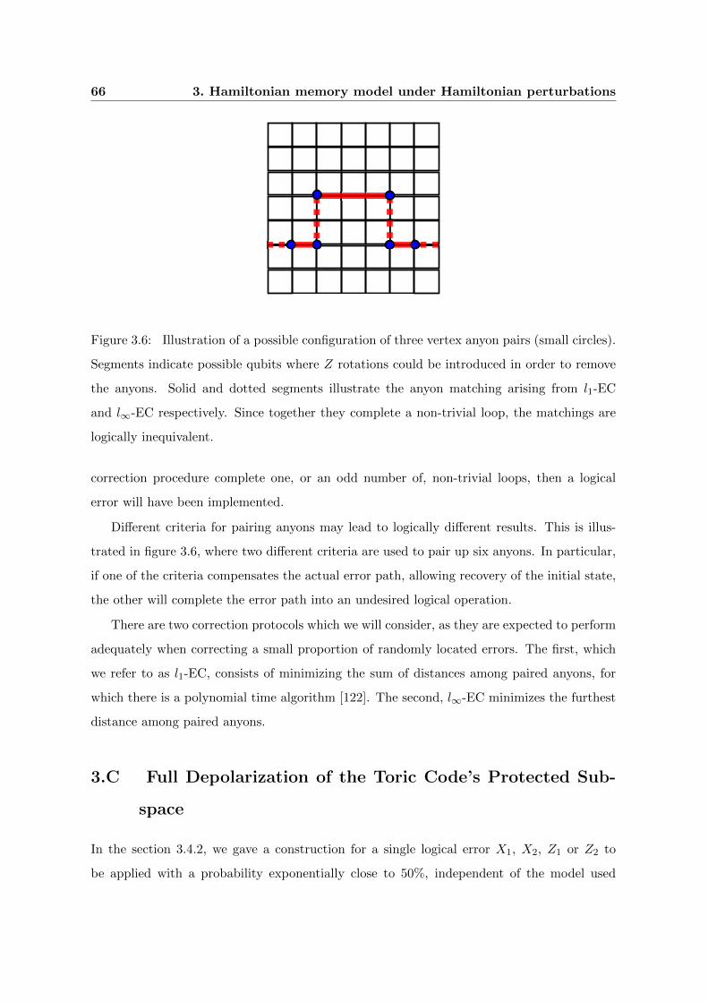
66 3. Hamiltonian memory model under Hamiltonian perturbations
Figure 3.6: Illustration of a possible configuration of three vertex anyon pairs (small circles).
Segments indicate possible qubits where Z rotations could be introduced in order to remove
the anyons. Solid and dotted segments illustrate the anyon matching arising from l1-EC
and l∞-EC respectively. Since together they complete a non-trivial loop, the matchings are
logically inequivalent.
correction procedure complete one, or an odd number of, non-trivial loops, then a logical
error will have been implemented.
Different criteria for pairing anyons may lead to logically different results. This is illus-
trated in figure 3.6, where two different criteria are used to pair up six anyons. In particular,
if one of the criteria compensates the actual error path, allowing recovery of the initial state,
the other will complete the error path into an undesired logical operation.
There are two correction protocols which we will consider, as they are expected to perform
adequately when correcting a small proportion of randomly located errors. The first, which
we refer to as l1-EC, consists of minimizing the sum of distances among paired anyons, for
which there is a polynomial time algorithm [122]. The second, l∞-EC minimizes the furthest
distance among paired anyons.
3.C Full Depolarization of the Toric Code’s Protected Sub-
space
In the section 3.4.2, we gave a construction for a single logical error X1, X2, Z1 or Z2 to
be applied with a probability exponentially close to 50%, independent of the model used
3.C Full Depolarization of the Toric Code’s Protected Subspace 67
for error correction. This is not sufficient to show that we get full depolarization of the
two-qubit subspace because it is not automatically clear that all 4 logical errors can be
introduced simultaneously in the same model; the problem being that crossing paths for anti-
commuting operations do not necessarily have a well-defined phase, and the perfect state
transfer operations can fail. Indeed, if two non commuting anyon propagation paths of equal
length cross at their midpoints, the amplitude corresponding to full propagation on both paths
can be seen to be 0 at times! It is the aim of this section to extend the setting of (Sec. 3.4.2) to
multiple logical errors while ensuring that the failure probability remain exponentially small
with system size, thereby allowing a fully depolarizing map on the code-space with probability
exponentially close to 1.
The basic idea behind this construction is that, for large systems, the propagation of
the anyons is essentially ballistic. Hence, we can divide our lattice into sections, and ensure
that the paths for anyons of different types only cross in regions where we can be (almost)
guaranteed of the order in which the anyons pass through. It is then our task to bound the
error probability.
Let us first consider the probability ps(t) of finding a propagated anyon at site s after a
propagation time t which is given in [70] as
ps(t) = f(s;D, sin2 t) = sin2s t cos2(D−s) t
(D
s
), (3.64)
where f is the binomial distribution function and D is the propagation length (i.e. there are
D + 1 possible anyon sites in the path). Here time has been normalized such that perfect
transfer occurs at t = π2 . Correspondingly, if P is the perfect transfer Hamiltonian for vertex
anyons and Π0 is the projector onto the subspace with a unique anyon at the transfer start
site, then
e−itPΠ0 =∑
s αs(t)Z⊗sΠ0
where |αs(t)| =√ps(t)
(3.65)
and Z⊗s is the tensor product of s consecutive Z operators along the anyon propagation path.
We are now in condition to compare an the actual evolution imposed by two non com-
muting anyon propagations |ψ(t)〉 and an ordered idealization of it |ψb;a(t)〉
|ψ(t)〉 = Ue−it(Pa+Pb)U† |ψ0〉|ψb;a(t)〉 = Ue−itPae−itPbU† |ψ0〉 .
(3.66)
68 3. Hamiltonian memory model under Hamiltonian perturbations
We will assume that the physical qubit corresponding to the crossing of both paths is between
anyon sites sa − 1 and sa of the anyon path associated to Pa and between anyon sites sb − 1
and sb of the anyon path associated to Pb. Furthermore, we will assume sa � sb, where what
is meant by (�) will soon be made clear. Under these conditions, we will see that |ψ(t)〉and |ψb;a(t)〉 are almost equal (at least during the time period corresponding to perfect state
transfer).
By definition, we have that 〈ψ(0)|ψb;a(0)〉 = 1. Let us now bound how fast this overlap
can actually decay
d 〈ψ(t)|ψb;a(t)〉d t
= i 〈ψ(t)| [Pb, e−itPa ]e−itPbU† |ψ0〉 . (3.67)
This allows bounding ∣∣∣∣d 〈ψ(t)|ψb;a(t)〉d t
∣∣∣∣ ≤ ∣∣∣[Pb, e−itPa ]e−itPbU† |ψ0〉∣∣∣ . (3.68)
Now let Π(a)∅ and Π
(a)0 be projectors onto the subspace with no anyons in the path of Pa
and the subspace where a single anyon is located at the initial site and define Π(b)∅ and Π
(b)0
analogously. Recalling that |ψ0〉 is a code state and our choice of rotation U , we have
(Π(a)∅ + Π
(a)0 )U† |ψ0〉 = U† |ψ0〉
(Π(b)∅ + Π
(b)0 )U† |ψ0〉 = U† |ψ0〉 .
(3.69)
Commuting these projectors and using the expansion (3.65) of the perfect transfer we may
express the RHS of equation (3.68) by∣∣∣∣∣[Pb,∑s
αs(t)Z⊗sΠ
(a)0 ]∑r
αr(t)X⊗rΠ
(b)0 U† |ψ0〉
∣∣∣∣∣ (3.70)
There is only one possible non commuting term in Pb and this only for s ≥ sa. Furthermore,
this term cancels for all but two terms in the sum over s′. We may then rewrite (3.70) as∣∣∣∣∣∣ 2Jsb∑
s≥sa αs(t)Z⊗sΠ
(a)0 ×
×(αsb(t)X
⊗sb−1 + αsb−1(t)X⊗sb)
Π(b)0 U† |ψ0〉
∣∣∣∣∣∣ (3.71)
Where Jsb is the strength of the term performing an anyon swap between sites sb and sb − 1.
Since each coefficient accompanies an orthogonal component of the state, we may recall the
definition in (3.65) and rewrite (3.71) as
2Jsb
√[psb−1(t) + psb(t)]
∑s≥sa
ps(t) sin2 ε, (3.72)
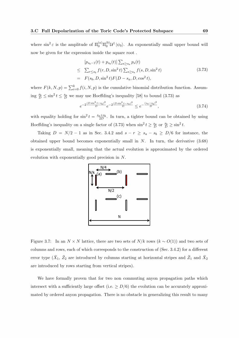
3.C Full Depolarization of the Toric Code’s Protected Subspace 69
where sin2 ε is the amplitude of Π(a)0 Π
(b)0 U† |ψ0〉. An exponentially small upper bound will
now be given for the expression inside the square root .
[psb−1(t) + psb(t)]∑
s≥sa ps(t)
≤ ∑r≤sb f(r,D, sin2 t)
∑s≥sa f(s,D, sin2 t)
= F (sb, D, sin2 t)F (D − sa, D, cos2 t),
(3.73)
where F (k,N, p) =∑k
i=0 f(i,N, p) is the cumulative binomial distribution function. Assum-
ing sbD ≤ sin2 t ≤ sa
D we may use Hoeffding’s inequality [58] to bound (3.73) as
e−2(D sin2 t−sb)
2
D e−2(D sin2 t−sa)2
D ≤ e−(sa−sb)
2
D , (3.74)
with equality holding for sin2 t = sa+sb2D . In turn, a tighter bound can be obtained by using
Hoeffding’s inequality on a single factor of (3.73) when sin2 t ≥ saD or sb
D ≥ sin2 t.
Taking D = N/2 − 1 as in Sec. 3.4.2 and s − r ≥ sa − sb ≥ D/6 for instance, the
obtained upper bound becomes exponentially small in N . In turn, the derivative (3.68)
is exponentially small, meaning that the actual evolution is approximated by the ordered
evolution with exponentially good precision in N .
Figure 3.7: In an N ×N lattice, there are two sets of N/k rows (k ∼ O(1)) and two sets of
columns and rows, each of which corresponds to the construction of (Sec. 3.4.2) for a different
error type (X1, Z2 are introduced by columns starting at horizontal stripes and Z1 and X2
are introduced by rows starting from vertical stripes).
We have formally proven that for two non commuting anyon propagation paths which
intersect with a sufficiently large offset (i.e. ≥ D/6) the evolution can be accurately approxi-
mated by ordered anyon propagation. There is no obstacle in generalizing this result to many
70 3. Hamiltonian memory model under Hamiltonian perturbations
such anyon paths, as required to introduce logical errors with high probability. Some leading
factors of order N2 appear but crucial factors remain exponentially decreasing in N .
In Fig. 3.7, we illustrate a configuration allowing the simultaneous introduction of all
possible logical errors by anyon propagation within the lattice. The marked stripes of width
N/k indicate locations where perpendicular anyon propagations begin or end. The pertur-
bation to be introduced is chosen randomly as in Sec. 3.4.2, such that each propagation
row/column starts with equal probability in either of each pair of opposing stripes. Taking
k fixed allows sufficiently many repetitions of the single row/column construction that the
probability of introducing each type of logical error approaches 12 exponentially fast with N .
Thus, after a perturbed evolution for time tf = O(N), and a final application of an arbitrary
error correcting protocol based on unperturbed syndrome measurement, the resulting state
is exponentially close to the maximally mixed state 11/4 of the code-space.
Chapter 4
Quantum memories based on
engineered dissipation
Storing quantum information for long times without disruptions is a major re-
quirement for most quantum information technologies. A very appealing ap-
proach is to use self-correcting Hamiltonians, i.e. tailoring local interactions among
the qubits such that when the system is weakly coupled to a cold bath the ther-
malization process takes a long time. Here we propose an alternative but more
powerful approach in which the coupling to a bath is engineered, so that dis-
sipation protects the encoded qubit against more general kinds of errors. We
show that the method can be implemented locally in four dimensional lattice
geometries by means of a toric code, and propose a simple 2D set-up for proof of
principle experiments.
4.1 Introduction
There are two existing approaches to providing coherent quantum storage on many-body
systems. The first one corresponds to fault tolerant quantum circuits[113, 47]. If one can
perform quantum gates and provide fresh initialized qubits with a sufficiently high accuracy
and frequency, then quantum computing and in particular, quantum memory is possible for
a time exponential in the dedicated resources.
More recently, Kitaev [32, 74] proposed that it might be possible to protect quantum
72 4. Quantum memories based on engineered dissipation
information passively by engineering of suitable Hamiltonian systems, in analogy to magnetic
domains for classical memories. While an energetically degenerate code subspace insensitive
to Hamiltonian perturbations is a necessary condition, it has become clear that there are
additional requirements for this approach to quantum memories to work. Possibly the most
important requirement is to cope with the undesired coupling between the storage system and
its environment. In this direction, the approach that has benefited from the most theoretical
progress goes by the moniker of self–correcting Hamiltonians, [11, 9, 53, 27].
For self–correcting Hamiltonians, a weak local coupling to a thermal bath is assumed.
Making a Born-Markov approximation, the evolution of the system can be described by a
thermalizing master equation. While for general local couplings, any initial state will decay to
the unique Gibbs state, it is still possible for the decay rate of specific observables to become
smaller as the number N of subsystems increases. This leads to the possibility of storing
quantum information by encoding it on a pair of slowly decaying anticommuting many-body
observables. A Hamiltonian will thus be called self–correcting provided that below a certain
finite bath temperature the dissipative dynamics leads to information lifetimes growing with
the system size (typically following an exponential increase). Alicky et al. [9] rigorously
proved an exponentially long relaxation time for protected observables in the 4D toric code.
Chesi et al. [26] generalized this result deriving a criteria for quantum memory based on
self–correcting Hamiltonians and lower bounds on the storage times. However, it is in general
not known how non thermal noise or even thermalization under a perturbed Hamiltonian
[104] affects this lifetime. In particular, this may be the case whenever the qubits are weakly
coupled to an additional bath which induces a small rate of depolarization[103].
Building on previous results, we propose and analyze an alternative way of protecting
quantum states. The method is similar to that of protecting Hamiltonians, but now the main
idea is to tailor the coupling of the qubits to a bath, so that the engineered dissipation extends
the life-time of the encoded qubit. Apart from being passive (i.e. not requiring the burden
of interrogating the quantum memory at intermediate times), the main advantage of this
scheme is that it can potentially correct for other kinds of errors beyond those generated by
thermalization, including depolarizing noise. In particular, we propose a specific method in
4 spatial dimensions inspired by toric codes and obtain evidence of its performance with the
help of numerical simulations. We also investigate a simplified 2-dimensional model protecting
4.1 Introduction 73
only from phase errors which could be a good candidate for proof of principle experiments.
Many-body classical memories based on dissipation (often under the name of asynchronous
celular automata) have naturally appeared in the context of classical fault tolerant computa-
tion. For example, using a simple local update rule on a 2D lattice, Toom [119, 50] showed
that classical information can be protected against weak local noise. A more elaborate update
rule by Gacs [41] provide protection even on a 1D lattice. These results already suggest that
dissipation may offer a powerful alternative to the existing methods for constructing many-
body quantum memories, as investigated in the present work. In fact, several authors have
already proposed the use of continuous quantum error correcting codes [105, 5, 109, 101, 87].
However previous works concentrate on a single level of error correction and do not address
the large N many-body scenario. A notable exception is the work of Dennis et al. [32] intro-
ducing a heat bath algorithm (thermal dissipation for the 4D toric code) in order to simplify
the efficacy analysis of a local many body quantum error correction algorithm. At the crux
of this approach is that thermal dissipation can be interpreted not only as introducing deco-
herence (errors), but also as performing a form of error correction, with the balance between
the two effects roughly given by the bath temperature. Indeed, this heat bath algorithm can
already be seen as a dissipative quantum memory lending itself to more natural engineering.
In fact, engineered dissipation is more general in that it need not satisfy detailed balance
conditions and thus its power extends that of cooling a self–correcting Hamiltonian. In other
words, the steady state need not be an equilibrium state and its dynamics may show a net
flow (imagine a funnel receiving water from a hose). As the classical results show, this more
general kind of dissipation may be crucial in order to correct general kind of errors.
Our proposal can be viewed as another example where engineered dissipation may be-
come a useful and alternative tool in the context of quantum information processing, beyond
quantum computation [125], state engineering [125, 34], or entanglement creation [76]. In all
those cases, it is desirable to be able to couple small subsets of qubits to Markovian environ-
ments so that their evolution equation follows a prescribed master equation. As exposed in
[125], dissipative gadgets provide a direct way of implementing this is in terms of damped
qubits; that is, a set of qubits which themselves follow a damping master equation due to
their coupling to an environment. Those qubits can be directly coupled to the physical qubits
of the quantum memory or computer to provide the desired dissipation, and thus appear as

74 4. Quantum memories based on engineered dissipation
an important resource in dissipative quantum information processing.
This chapter is organized as follows. In section 4.2 we briefly present the general idea of
engineered dissipative quantum memories. In section 4.3 we display two different but rather
obvious approaches to dissipative quantum memories and discuss why they are not entirely
satisfactory. In section 4.4 we present a specific method in 4 spatial dimensions as well as the
results of numerical simulations which validate the performance of the scheme. section 4.5
contains a simplified version in 2 spatial dimensions which corrects against phase errors and
that could be tested experimentally in the near future. In section 4.6 we show how one can
use dissipative qubits to engineer the dissipation and analyze under which condition one can
use them in this context. All previous section contain the main statements of our work. The
detailed proofs of our results and more thorough explanations are given in the appendices.
Figure 4.1: We assume that a piece of quantum information is encoded into a many body
system. The engineered dissipation, is then responsible for making the degrees of freedom
which carry the encoded quantum information resilient against the uncontrolled noise pro-
cesses taking place. Finally, the decoding process extracts the quantum information from the
collective degrees of freedom.
4.2 Statement of the problem
We consider a logical qubit encoded in N physical qubits, which are appropriately coupled to
an environment providing dissipation. We describe the action of the engineered environment,
as well as of the other sources of decoherence through a master equation
ρ = Ldiss(ρ) + Lnoise(ρ) (4.1)
Here, ρ is the density operator for the qubits, Ldiss the Liouvillian describing the engineered
dissipation, and Lnoise will denote a noise term contribution to the master equation. This
4.3 Straightforward QECC encoding 75
could be local depolarizing noise for instance
Lnoise(ρ) = ΓεLdep(ρ) = Γε
N∑n=1
1n
2⊗ trn(ρ)− ρ, (4.2)
or any other weak local noise term. Our goal is to show that for appropriate choices of Ldiss
we can extract the encoded qubit reliably after a time which substantially increases with N .
In general, any trace preserving dissipative master equation as Ldiss may be write in
Lindblad form [84]
ρ = L(ρ) = −i[H, ρ] +∑k
2Lkρ0L†k − {L
†kLkρ}+, (4.3)
consisting of a Hamiltonian term describing the unitary evolution, and a dissipative part
which may be written in terms of Lindblad or jump operators Lk. Furthermore, the models
of engineered dissipation we propose can be seen to adhere to a more benign form
ρ =∑l
Γl [Tl(ρ)− ρ] , (4.4)
where Tl are positive trace preserving channels. For these particular cases, the time dependent
density matrix may be given an explicit stochastic expansion in the form of
ρ(t) = e−Γt∞∑n=0
Tnρ(0)
n!, (4.5)
where Γ =∑
l Γl and T (ρ) =∑
l ΓlTl(ρ). This stochastic expansion will be useful for both
proofs and Monte Carlo simulations.
4.3 Straightforward QECC encoding
Here we introduce and analyze two straightforward methods of encoding a QECC in the
dissipation. The first one consist of coupling all the qubits with a reservoir in such a way
that each application of a jump operator a whole error correction procedure takes place. In
the second, we encode the QECC in several Lindblad terms, so that each jump correspond
to an execution of a part of the QEC. The main purpose of this section is to show that those
simple approaches do not work as one could imagine, and thus it illustrates why the design
of engineered quantum memories is not a trivial task. Both approaches require multibody
coupling to a single environment, where the number of system qubits coupled to the same
76 4. Quantum memories based on engineered dissipation
damped qubit grows with N , the size of the memory. In principle perturbation theory gadgets
allow the engineering of such terms, provided their respective intensity decay exponentially
with the number of subsystems involved. Not withstanding, a strength increasing with N
would be required to make the first approach work, while in the second approach only a
polynomial decrease with the number of subsystems involved would preserve functionality. In
the next section we will present a scheme which circumvents these problems, although still
with the caveat that it requires non-local couplings (as it works in 4 spatial dimensions).
4.3.1 Single Jump Operator
One major obstacle to traducing the usual error correction strategies to a dissipative scenario
is due to the random times at which dissipative terms enact the recovery operations. We
illustrate this problem in the case of a straightforward approach to dissipative protection.
One can always implement in the dissipative Liouvillian a standard quantum error correction
procedure which preserves the logical qubit: Ldiss(ρ) = Γ[R(ρ)−ρ], where R is a full recovery
operation and Γ adjusts the rate at which the recovery operation is applied (imagine full
correction of an N qubit QECC). Apart from the unrealistic nature of highly many–body
dissipation terms required in this construction, it is easy to see that it does not serve our
purposes. The reason can be seen by unraveling the quantum jump operators [25], there is
a finite N independent probability for more than 1Γε
time to elapse until the next recovery
operation. Such long times allow too many errors to accumulate for any QECC to recover
with high fidelity.
The alternative is to have dissipation implement many independent processes instead of
a single monolithic error correction procedure. Ideally, having independent processes take
care of removing independent error sets can make the accumulation of a critical fraction
of errors exponentially unlikely. The difficulty of having independent dissipation processes
is that contrary to the circuit model the order of their application is not enforced in any
way. Thus, directly encoding each gate of a QECC recovery circuit into a dissipation term
generally leads to a meaningless evolution. However, we will show that in specific cases where
dissipation terms commute or show some order property lending itself to rigorous analysis,
the asynchronous nature is not an obstacle.
4.3 Straightforward QECC encoding 77
4.3.2 Concatenated QECC Dissipation
It is indeed possible to design a many-body dissipative quantum memory. The strategy is
to take the dissipation term as a sum of recovery operations occurring on different groups
of qubits. Those operations correspond to recovery of the different logical qubits at each
level of a simple concatenated QECC [75]. Intuitively, one may argue that the difficulty
of implementing a given dissipation term increases with the number of qubits involved. We
attempt to compensate for this difficulty by imposing that the operator norm required for such
Lindblad terms decays with a power law respect to the number of physical qubits involved.
More specifically, we take
Ldiss(ρ) = Γ∑l,n
δM−l[Rl,n(ρ)− ρ]. (4.6)
Here, l = 0, 1, . . . ,M − 1 denotes the level of concatenation, and n further specifies on which
set of qubits the recovery operations Rl,n are applied. In appendix 4.C, we show that if the
local noise rate Γε is sufficiently small then initially encoded information is lost at a rate which
is exponentially small with respect to the number of qubits used (i.e. double exponentially
small with the level of concatenation M). The weakness condition on the noise can be made
precise by
Γε < Γ?ε =δ2Γ
k2, (4.7)
where k is the number of physical qubits in the code to be concatenated. Assuming the
perfect 5 qubit QECC and taking the strength of many body terms inversely proportional to
the number of bodies (δ = 1/5), a threshold of Γ?ε = 1.6 × 10⁻³Γ is obtained for the noise
rate. When the error rate is below the error threshold, the relaxation rate for the encoded
information has an exponentially small upper bound given by
τ−1 ≤ ΓεδM
(ΓεΓ?ε
)2M−1
(4.8)
The above scheme is mainly of formal interest, since the non local recovery operations
encoded in the dissipative master equation require many qubits at different locations to in-
teract with the same environment. While the necessary scaling of such terms needs to be
polynomial for our proof to go through, the derivation of such terms based on effective many-
body Hamiltonians and the dissipative gadgets we propose is expected to decay exponentially
with the number of bodies involved. Even more realistically, one would expect many-body

78 4. Quantum memories based on engineered dissipation
dissipation terms to cope with many body error terms arising from imperfect implementation.
In practice, it would be desirable to find a set up where the dissipation terms are spatially
localized by considering the qubits arranged in a lattice.
4.4 Local dissipative protection in 4D
In classical systems Toom’s rule [119] has been proven to be a simple translationally invariant
update rule in a 2D Periodic Boundary Condition (PBC) lattice which is capable of preserving
classical information, provided that the noise contribution to the dynamic is sufficiently weak.
While we have not been able to extend this rule for quantum protection in 2D, we will consider
a quantum analog of Toom’s rule for 4D. The underlying QECC used is the 4D toric code, a
stabilizer quantum error correcting code with 6 body stabilizer generators which can be made
spatially local in a 4D PBC lattice. Dennis et al.[32] proposed it as a local QECC, and the
corresponding stabilizer Hamiltonian was recently rigorously proven to be self–correcting by
Alicki et al. [9]. We derive a local master equation for protecting information encoded into
the 4D toric code based on a Toom like rule introduced by Ahn [6] and study its efficiency
for protecting encoded observables. We then consider the protection process and numerically
study the lifetime of information when depolarization errors are introduced extensively at a
small yet constant rate.
A fully rigorous description of the QECC and the local update rule used is provided in
the appendix 4.B. For the moment it is sufficient to specify that the master equation has the
form of eq. (4.1) where the specific Ldiss used associated to the 4D toric code will be called
L4D-TCToom and Lnoise is weak extensive depolarizing noise as in eq. (4.2). The numerical
results (Fig. 4.2) strongly support the existence of a critical error rate Γ?ε ≈ 0.004×Γ ( where
Γ is the correction rate to be specified ) below which, the lifetime of the encoded information
increases exponentially with the lattice size.
Although the results above have no obvious practical implication, they suggest that local
models may exist in spatial dimensions lower than 4 (for the search of quantum memories
based on protecting Hamiltonians in lower dimension see [11, 27, 53]). The hope, is that even
if self-correcting quantum memories fail to exist in lower dimensions, the use of engineered
dissipation may still provide a solution.
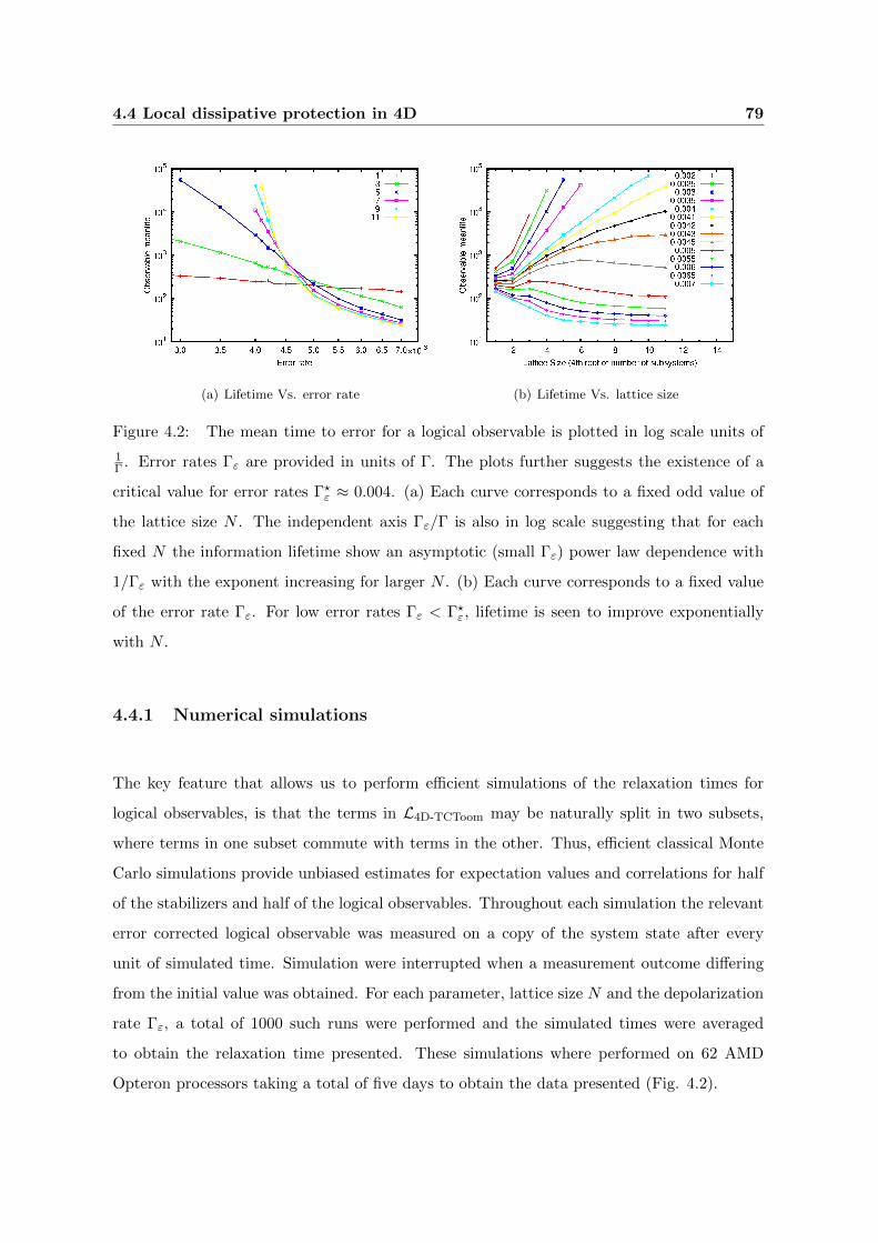
4.4 Local dissipative protection in 4D 79
(a) Lifetime Vs. error rate (b) Lifetime Vs. lattice size
Figure 4.2: The mean time to error for a logical observable is plotted in log scale units of
1Γ . Error rates Γε are provided in units of Γ. The plots further suggests the existence of a
critical value for error rates Γ?ε ≈ 0.004. (a) Each curve corresponds to a fixed odd value of
the lattice size N . The independent axis Γε/Γ is also in log scale suggesting that for each
fixed N the information lifetime show an asymptotic (small Γε) power law dependence with
1/Γε with the exponent increasing for larger N . (b) Each curve corresponds to a fixed value
of the error rate Γε. For low error rates Γε < Γ?ε, lifetime is seen to improve exponentially
with N .
4.4.1 Numerical simulations
The key feature that allows us to perform efficient simulations of the relaxation times for
logical observables, is that the terms in L4D-TCToom may be naturally split in two subsets,
where terms in one subset commute with terms in the other. Thus, efficient classical Monte
Carlo simulations provide unbiased estimates for expectation values and correlations for half
of the stabilizers and half of the logical observables. Throughout each simulation the relevant
error corrected logical observable was measured on a copy of the system state after every
unit of simulated time. Simulation were interrupted when a measurement outcome differing
from the initial value was obtained. For each parameter, lattice size N and the depolarization
rate Γε, a total of 1000 such runs were performed and the simulated times were averaged
to obtain the relaxation time presented. These simulations where performed on 62 AMD
Opteron processors taking a total of five days to obtain the data presented (Fig. 4.2).
80 4. Quantum memories based on engineered dissipation
4.5 Accessible toy model
As a a proof of principle, we now present an engineered dissipation toy model providing
protection for quantum information. One can implement the underlying ideas of dissipative
quantum memories with 2D lattices at the expense of being able to correct only for dephasing
noise
Lphase(ρ) = Γzε
N∑n=1
σzn(ρ)σzn − ρ. (4.9)
Given a noise model including only one type of error (such as σz phase errors) we will be able
to cast a classical memory prescription into a quantum scenario. A first step, is to define two
logical observables
ZEC ≡⊗s
σzs XEC ≡ θ(∑
s
σxs
)(4.10)
where θ is the Heaviside step function. The first observable ZEC commutes with the noise
Lphase and is thus completely immune to it. The noise can only change the value of XEC ,
for the part of ρ which is in the ±1 eigenspace of∑
s σxs (i.e. states for which the absolute
magnetization in the X direction is minimal). Dissipation will protect the XEC observable
by keeping most of ρ in a high X magnetization subspace. The master equation ρ = LNN(ρ)
for nearest neighbor majority voting is written as a Liouvillian in Lindblad form [84] as
LNN(ρ) = Γ∑
<s,r,t>
Ls,r,tρL†s,r,t −
1
2{L†s,r,tLs,r,t, ρ}+, (4.11)
where the index s runs over all sites, r 6= t are nearest neighbors of s and the Lindblad
operators are given by
Ls,r,t ≡ σzs1− σxs ⊗ σxr
2
1− σxs ⊗ σxt2
. (4.12)
This is, the first factor performs a phase flip when the second and third factors (projectors)
are non zero (i.e. when site s points differently than its two neighbors r and t). The Lindblad
operators are designed such that they also commute with ZEC and can only change XEC in
the portion of ρ with minimal X magnetization.
The stability of the XEC observable in such an evolution can be mapped to magnetization
metastability in classical studies [18, 30]. Restricting r and t to be north and east neighbors
in an N×N PBC lattice, one recovers Toom’s rule [119, 50] which is proven to provide an ex-
ponential survival time, even in the presence of biased errors. However, the PBC requirement
is experimentally unrealistic.
4.6 Dissipative gadgets 81
We numerically consider an experimentally accessible setup which does not require peri-
odic boundary conditions. Physical qubits will be located on an N × N 2D square lattice
sites. The sites r and t are taken among all possible nearest neighbors of s. The number of
valid neighbor combinations are(
42
)= 6 for inner sites s,
(32
)= 3 for lattice border sites s and
only one combination for corner sites. In the following plot (Fig. 4.3), we show how having
a protective dissipation term LNN can increase the relaxation time of XEC , a many-body
encoded observable (red). This is in contrast to the complementary observable which does
not benefit from dissipative protection. On the contrary, given any depolarization rate, the
relaxation time of ZL decreases with the inverse of the number of physical qubits involved
(blue).
4.6 Dissipative gadgets
As we have shown, the possibility of controlled quantum dissipation opens a host of new pos-
sibilities for QIP [34, 125, 76]. However, while some naturally occurring forms of dissipation
may be readily exploited, it is crucial to have a systematic way of engineering arbitrary dissi-
pative dynamics. A way of achieving complete control over the dissipation is to be capable of
engineering independent Lindblad jump operators while keeping their interference with each
other weak. For this we must assume availability of many body Hamiltonians, achievable
through perturbation theory gadgets [64, 19] and of some naturally occurring dissipation,
namely in the form of damped qubits. We apply the approximation of independent rates of
variation [31] pg. 356 on the damped qubits which requires the bath correlation time for the
damping process to be much shorter than the inverse of any coupling constant in the system.
Coupling to these damped qubits can thus be seen as a resource in the design of quantum
dynamics, analogous to freshly initializing qubits in quantum circuits.
Coupling the system to a damped qubit ancillary degree of freedom was proposed as a
possible path to engineer arbitrary effective dissipative dynamics [125]. More specifically, the
Hamiltonian coupling H = ω(L ⊗ σ+ + L† ⊗ σ−) to an ancilla with damping rate γ leads
to an effective dissipative dynamics of the system corresponding to the Lindblad operator
ω√
2/γL. Here σ− = |0〉 〈1| and σ+ = |1〉 〈0|.In order to use these dissipation gadgets as basic building blocks in more complex scenar-
ios, it is essential to make explicit possible limitations and restrictions of the implemented

82 4. Quantum memories based on engineered dissipation
Figure 4.3: Relaxation time for ZEC (red curves) and XL (blue curves) in units of Γ−1.
Each red curve presents the relaxation time τZ (numerically obtained) corresponding to one
value of the relative dephasing rate Γ/Γphase given by the intercept at N = 1. Blue curve
have the functional form τX = Γ−1dep ∗N−2 and each corresponds to one value of Γ/Γdep also
given by the intercept at N = 1. The lifetime τ of the encoded logical qubit can be seen
to be estimated by τ ≈ min{τX , τZ}. Given Γ/Γdep and Γ/Γphase, one may intersect the
corresponding curves to obtain the value of N leading to the optimal qubit lifetime τ . For
example, if Γdep = 5×10⁻⁵Γ and Γphase = 0.1Γ the optimal lattice size of 4×4 allows a ×100
increase in the quantum information relaxation time τ . A more extreme case may be seen
when Γphase = 0.01Γ and Γdep ≤ 5 × 10⁻⁵Γ where a factor ×50 is gained by simply using a
2× 2 lattice.
dissipation. In appendix 4.A we provide a detailed derivation of the effective system dy-
namics which makes three main contributions to our understanding of dissipative gadgets.
Firstly, while the usual approach of adiabatic elimination obtains an effective dynamics in
terms of a coarse grained time, our derivation shows that excluding a short initial transient
period, this temporal coarse graining is not necessary. Secondly, we provide explicit bounds
on the deviation from the desired state and instantaneous dynamics which are accompanied
by a smallness prefactor (ω/γ)2. Finally, we include an independent internal dynamic for
the system, and show, that the resulting effective dissipation carries through essentially un-
affected provided the strength of the internal dynamics is sufficiently weak. While the last

4.7 Conclusions and perspectives 83
point already suggests that the extensive application of local dissipation gadgets should be
well behaved, a fully rigorous analysis is beyond the scope of this thesis.
4.7 Conclusions and perspectives
We have introduced engineered dissipation as a tool to protect against general quantum noise
and proposed examples providing protection from local noise. In the case of concatenated code
dissipation, we prove that information can be made resilient against any strictly local noise.
Numerical simulations with depolarizing noise strongly suggest dissipative protection may be
made spatially local in 4D. For purely dephasing noise we propose a dissipative protection
scheme local in 2D. Proof of principle experiments could be realized with trapped ions, or
atoms in optical lattices.
A self-correcting thermalization scheme associated to the 4D toric code Hamiltonian can
provide encoded quantum information similar protection against depolarizing noise. In this
sense, we have not illustrated the advantage of engineered dissipation. While the approach we
have taken with the 4D TC is analogous to Toom’s 2D update rule for classical information
the thermalization of the 4D toric code can be seen as analogous to thermalization of the 2D
Ising model respect to unbiased noise. However, stretching such parallelism with the classical
problem suggests that engineered dissipation may be strictly more powerful and that it may
be possible to engineer a 2D local dissipation mechanism capable of protecting quantum
information. Indeed, while in 1D there can not be a self-correcting classical memory, a 1D
local dissipative master equation due to Gacs [41] is proven to provide increased classical
information lifetime with the chain size. Inspired by Gacs’ construction, Harrington [55]
has proposed a local quantum error correction scheme in 2D capable of protecting against
quantum errors. To make this into a dissipative scheme, the requirements of a) a global
synchronization clock, b) logarithmically increasing local storage space c) error free evolution
of classical information, all need to be relaxed. Whether these assumptions can be relaxed,
or other schemes in 2D or 3D exist are important questions that may dictate the fate of the
practical applications for dissipative quantum memories.

84 4. Quantum memories based on engineered dissipation
4.A Adiabatic elimination of ancilla
In this section, we prove that Master equations with arbitrary Lindblad operators may be
engineered to high accuracy by coupling the system to ancillary resource qubits which are
themselves being cooled. The basic idea is to extend the system with an additional binary
degree (spin 1/2) of freedom per Lindblad operator L to be implemented. These degrees of
freedom are further assumed to be strongly dissipatively driven with a rate γ into a |0〉 〈0|ground state. We will show that a target dissipative evolution composed of a single Lindblad
jump operator
Ltarget(ρ) = LρL† − 1
2
{L†L, ρ
}+, (4.13)
may be implemented within a small error margin. The technique used for the proof follows
the adiabatic elimination of the excited ancilla subspace in spirit, but takes into account
corrections in order to provide rigorous bounds on the deviations from the intended evolution.
Our derivation starts by assuming that the full dynamics of the system can be written as
ρ = −i[H, ρ] + 2γσ−ρσ+ − γ{σ+σ−, ρ
}+
+ γLsys(ρ) (4.14)
where σ+ = |1〉 〈0|A and σ+ = |1〉 〈0|A are raising and lowering operators on the ancilla qubit
and the Hamiltonian H couples the system to the ancilla
H = ω(L⊗ σ+ + L† ⊗ σ−) (4.15)
and Lsys is an additional evolution term with no effect on the ancillas. Here, the assumption
that is implicitly being made, is that we may independently sum the interaction Hamiltonian
H to the dissipative dynamics on both the system and the ancilla. In the case of the ancilla
decay this is the approximation of independent rates of variation [31] pg. 356, which assumes
correlation times for the reservoir responsible for spontaneous decay to be much shorter than
any other relevant time in the system. An important example where this approximation
holds to a great degree of accuracy is for two level atoms at optical frequencies, where the
autocorrelation time of the coupled vacuum fluctuations can be as much as ten orders of
magnitude shorter than the inverse of any of the other coupling constants. Since our derivation
for the weak system Liouvillian does not require temporal coarse graining, the successively
incorporation of Hamiltonian interactions rigorously leads to the additive appearance of the
desired Liouville terms up to leading order. Assuming ε = ω/γ � 1 we can rescale to a

4.A Adiabatic elimination of ancilla 85
unitless time by incorporating a factor γ leading to the following differential equations for the
reduced density matrices.
ρ00 := 〈0| ρ |0〉 = 2ρ11 − iεL†ρ10 + iερ01L+ Lsys(ρ00) (4.16)
ρ01 := 〈0| ρ |1〉 = −ρ01 + iερ00L† − iεL†ρ11 + Lsys(ρ01) (4.17)
ρ11 := 〈1| ρ |1〉 = −2ρ11 − iεLρ01 + iερ10L† + Lsys(ρ11) (4.18)
From here, we may obtain the integral forms
ρ01(τ) =e−τρ01(0) +
∫ τ
0e−t
′Lsys[ρ01(τ − t′)]dt′ (4.19)
+iε
∫ τ
0e−t
′[ρ00(τ − t′)L† − L†ρ11(τ − t′)]dt′
ρ11(τ) =e−2τρ11(0) +
∫ τ
0e−2t′Lsys[ρ11(τ − t′)]dt′ (4.20)
−iε∫ τ
0e−2t′ [Lρ01(τ − t′)− ρ10(τ − t′)L†]dt′
Assuming the initial conditions ρ01(0) = ρ11(0) = 0, that ‖L‖ ≤ 1 and ‖Lsys‖ ≤ Eε2, and
using that ‖ρ00‖+ ‖ρ11‖ ≤ 1 we may bound
‖ρ01(τ)‖ ≤ ε and ‖ρ11(τ)‖ ≤ ε2, (4.21)
with ε = ε1−Eε2 . It is now straightforward to bound ‖ρ00(τ)‖ ≤ (4 + E)ε2. We may now
concentrate on tighter bounds composed of higher order terms in ε but also, of exponentially
decaying terms. A first step to do this is to perform integraton by parts; on eq. (4.19) one
obtains
ρ01(τ) =iερ00(τ)L† − iεe−τρ00(0)L† (4.22)
−iε∫ τ
0e−t
′[ρ00(τ − t′)L† + L†ρ11(τ − t′)
]dt′
+
∫ τ
0e−t
′Lsys[ρ01(τ − t′)]dt′.
In the case of ρ11 we straightforwardly obtain
ρ11(τ) =− iε
2Lρ01(τ) (4.23)
+iε
2
∫ τ
0e−2t′Lρ01(τ − t′)dt′ + h.c.
+
∫ τ
0e−2t′Lsys[ρ11(τ − t′)]dt′

86 4. Quantum memories based on engineered dissipation
This expression may be massaged into a form which may be more readily bounded. The steps
involved include, expanding ρ01 according to eq. (4.17), then expanding appearances of ρ01
according to eq. (4.22) and finally integrating numerical factors and grouping terms. After
such manipulation, one reaches the expression
ρ11(τ) =ε2
2
[Lρ00(τ)L† − e−τ (2− e−τ )Lρ00(0)L† (4.24)
−∫ τ
0e−t
′(2− e−t′)Lρ00(τ − t′)L†dt′
−∫ τ
0e−t
′(2− 2e−t
′)LL†ρ11(τ − t′)dt′
]+ h.c.
+iε
2
∫ τ
0e−2t′LLsys[ρ01(τ − t′)]dt′ + h.c.
+
∫ τ
0e−2t′Lsys[ρ11(τ − t′)]dt′
Using eqs. (4.22) and (4.24), one may prove the following higher order bounds
‖ρ01 − iερ00L†‖ ≤ (2E + 5)ε3 + εe−τ (4.25)
‖ρ11 − ε2Lρ00L†‖ ≤ (3E + 7)ε4 + 2ε2e−τ , (4.26)
Inserting these bounds into the definition of ρ00 we may bound deviation from the target
evolution by
‖ρ00 − 2ε2Ltarget(ρ00)− Lsys(ρ00)‖ ≤ (10E + 24)ε4 + 4ε2e−τ (4.27)
After a short transient time of the order 1γ log 1
ε , the exponential term can be neglected.
Furthermore, note that the internal system dynamics Lsys may be time dependent and thus
encode correlations of different components of the system in its time dependence.
4.B 4D Toric code
4.B.1 The 4D Toric code as a stabilizer code
We will now provide an informal description of the 4D toric code. For every vertex of an
N ×N ×N ×N lattice, there are 6 orientations of faces on which physical qubits are located.
Thus, the 6×N4 physical qubits are arranged on the 2D faces of a 4D PBC lattice. We can
now introduce an over-complete set of local stabilizer generators for the code, half of which
correspond to 1D edges, the other half corresponding to 3D cubes. For each 1D edge, there
4.B 4D Toric code 87
is a tensor product operator Z⊗6, the product of Z operators acting on the six 2D faces to
which this edge belongs. Dual to this, for each 3D cube, there is a tensor product operator
X⊗6, the product of X Pauli operators over the six 2D faces of the cube. Two edge and cube
stabilizers overlap iff the edge is an edge of the cube, and then their overlap will be in exactly
two faces. Thus all stabilizer generators are seen to commute.
4.B.2 Logical degrees of freedom
Counting of the remaining degrees of freedom additional to the stabilizer syndrome obtained
is not as straightforward as for the 2D toric code, where every syndrome with an even number
of anyons was possible. In the 4D case, the required condition is that the set of unsatisfied
stabilizers is only allowed to be a combination of closed loops (in the lattice and dual lattice
respectively). However, one can explicitly construct six pairs of anticommuting logical op-
erators which commute with all stabilizer terms, one pair for each of the six possible plane
orientations. From each pair, one operator is a full plane of X rotations along a full plane
wrapping around the grid in one of the six possible orientations. The second operator from
each pair consists of a dual plane of Z operators arranged along the perpendicular plane
orientation. Although analogous to the logical operators on the 2D toric code, this image
probably stretches our 2D or at most 3D imagination. Thus, to obtain an intuition about
this construction it is convenient to provide formal expressions which one may operate with.
4.B.3 4D PBC lattice notation
Each vertex of the 4D periodic lattice can be identified by a four component vector ~v =
v0, v1, v2, v3 ∈ Z4N . For each vertex ~v, there are four edges e, six faces p and four cubes c
having the vertex as a lower corner. These orientations may be described by four component
binary vectors
e, p, c ∈ {(v0, v1, v2, v3) | vi ∈ {0, 1}}, (4.28)
with edge e, face p, or cube c orientations satisfying the additional condition∑3
i=0 vi equal
to 1, 2 or 3 respectively. Each physical qubit can be identified with a tuple ~v, p, where p
identifies the plane orientation and ~v its lower side corner. The Z type edge stabilizers E~v,e

88 4. Quantum memories based on engineered dissipation
are given by
E~v,e =⊗e⊂p
Z~v,p ⊗ Z~v−p+e,p, (4.29)
with six participating physical qubits. Finally, the X type cube stabilizer C~v,c are given by
C~v,c =⊗p⊂c
X~v,p ⊗X~v+c−p,p, (4.30)
also with six participating physical qubits.
We will now describe a set of logical operators commuting with all stabilizers which will
be used to encode information in absence of errors. There is one pair of such anticommuting
logical operators for each plane orientation p and they are given by
XLp =
N⊗n,m=1
Xne1+me2,p ZLp =
N⊗n,m=1
Zne3+me4,p, (4.31)
with e1 + e2 ≡ p and e3 + e4 ≡ p⊥. It is easy to see that according to this definition, the
two logical operator XLp and ZLp anticommute, as they coincide only at qubit (~0, p). One can
further verify that such operators commute with the complete set of stabilizers. Finally, it is
not hard to see, that if one assumes the state to be in the code subspace (i.e. +1 eigenstate
to all stabilizers), then any homologically equivalent surfaces results in equivalent definition
for the operators.
4.B.4 4D Quantum Toom’s rule
We now define a local update rule which will later be used in two ways, first as a dissipa-
tion mechanism capable of keeping errors from accumulating too badly, second as the basic
component of an information recovery procedure permitting removal of all errors to allow
information read-out. The update rule is analogous to Toom’s rule for classical information
stored in a 2D lattice. While the prescription of Toom’s rule is to flip a bit if it is different to
both its two lower side neighbors, the prescription in 4D will be to X “flip” a qubit if both its
neighboring lower side Z edge stabilizers are not satisfied, but also to Z “flip” a qubit if both
its lower side X cube stabilizers are not satisfied. This is, a local rotation may be performed
depending on neighboring stabilizer state. This is in complete analogy to an interpretation of
Toom’s rule in terms of local stabilizers. One property that permits analytic and numerical
analysis of such a scheme is the decoupling of recovery for X and Z logical operators.
4.B 4D Toric code 89
For each qubit (~v, p), we can write the super-operator describing the quantum jump im-
plementing the update rule as
RZ~v,p(ρ) = Z~v,pPX~v,pρP
X~v,pZ~v,p + PX⊥~v,p ρP
X⊥~v,p (4.32)
where PX~v,p is the projector onto the subspace where a Z flip should be performed on qubit
(~v, p) and PX⊥~v,p the orthogonal subspace. Assuming p = e1 + e2 the projector may be defined
as
PX~v,p =1
4(1− E~v,e1)(1− E~v,e2). (4.33)
Analogously, one may define an update rule RX~v,p which in a similar way, introduces an X
“flip” depending on the corresponding projectors PZ~v,p in terms of Z type stabilizers.
4.B.5 Full recovery and error corrected operators
The superoperators RZ~v,p and RX~v′,p′ always commute. Only recovery operators of the same
kind may lack commutation when considering neighboring plaquetes. In particular, to define
a full recovery operation R in terms of these local recovery update rules, it is necessary
to unambiguously specify an order of application. Indeed, in our simulation code, a sweep
through the lattice is taken as this order and we observe a good performance in recovering the
originally encoded observables (Fig. 4.4). Once the recovery operation R is unambiguously
specified, it is possible to define robust logical observables XECp and ZECp such that
tr(ZECp ρ) = tr(ZLp Rρ) tr(XECp ρ) = tr(XL
p Rρ). (4.34)
Or more compactly
ZECp = R(ZLp)
and XECp = R
(XLp
). (4.35)
Thus, error corrected logical observables (super-index EC), provide a robust result when
evaluated on a state with sufficiently few errors and coincide with logical operators on the
error-free subspace.
4.B.6 Master equation
We study a master equation including a locally depolarizing noise term of strength Γε, and
the proposed Lindblad terms intended to avoid error clusters from growing. The simulated

90 4. Quantum memories based on engineered dissipation
Figure 4.4: Recovery probability of an encoded observable in the 4D toric code is plotted as a
function of depolarization probability per qubit. Odd lattices sizes from 1 to 11 are represented
in the different curves and suggest a critical depolarization probability of approximately 7.5%.
master equation may be written as
ρ = Lρ = ΓL4DToomρ+ ΓεLdepρ (4.36)
where the dissipative protection L4DToom is given by
L4DToomρ =∑~v,p
LX~v,pρLX†~v,p −
1
2
{LX†~v,pL
X~v,p, ρ
}+
+LZ~v,pρLZ†~v,p −
1
2
{LZ†~v,pL
Z~v,p, ρ
}+.
(4.37)
The protecting Lindblad operators are
LZ~v,p = Z~v,pPX~v,p LX~v,p = X~v,pP
Z~v,p, (4.38)
corresponding to the Toom like quantum jump superoperators R{X,Z}~v,p introduced in Eq. 4.32.
We perform numerical experiments to determine the relaxation time for logical observables
(i.e. tr[XECρ(t)] ≡ tr[XLRρ(t)].) Evolutions are taken to start in a code state with an
unambiguous XL or ZL logical value and consistency of the error corrected logical observables
are checked regularly in time. The mean time to the first change in the value observed for
XEC or ZEC is taken as an estimator of the relaxation time.

4.C Concatenated-code dissipation 91
4.B.7 Numerical considerations
Evolution under this master equation can be numerically simulated efficiently for a commuting
set of observables such as the edge stabilizers and a commuting set of logical observables. This
means that a classical Monte Carlo simulation is enough to study the probability of obtaining
the correct outcome when measuring distinct logical observables which were initially well
defined. The results of such simulations are presented in (Fig. 4.2) for different sizes of the
lattice grid up to 11 and different values for Γε. These suggest a critical value for the noise
rate Γ?ε ≈ 0.004, below which arbitrarily long relaxation times may be achieved by increasing
the lattice size. Given that below threshold error rates, the information lifetime seems to
grow exponentially with the lattice size, and that the simulation time per unit time is also
proportional to the fourth power of the lattice size, it is numerically costly to extend our
evidence to larger lattices.
4.B.8 Definition of efficient recovery R
To check whether the encoded observable is still recoverable at time t, we apply a correction
super-operator R on ρ(t). The definition of R consists of sequentially applying the local jump
superoperators R{X,Z}~v,p in a sweeping order. This shows a high performance for removing all
error domains (i.e. it presents a numerical threshold to depolarizing noise on up to ≈ 7.5%
of the qubits as shown in (Fig. 4.4) .) Furthermore, computer simulations of R are efficient,
requiring a minimal amount of O(N4) operations. This is important since the Rρ(t) must
be checked every unit time to obtain an estimate of the relaxation times of error corrected
logical observables.
4.C Concatenated-code dissipation
Paz and Zurek [105] presented the first studies of protecting quantum information through
the use of a continuous dissipative process. They introduce a general master equation form
for the class of stabilizer QECC and analyze their performance in some simple cases. In
this section, we will adapt their construction and propose master equations for concatenated
QECC which are provably robust against sufficiently weak local noise.
92 4. Quantum memories based on engineered dissipation
For stabilizer QECC, the recovery super-operator R can be written in Kraus form as
R(ρ) =∑(m)
R(m)P (m)ρP (m)†R(m)†, (4.39)
where P (m) are projectors onto orthogonal syndrome subspaces with∑
(m) P(m) = 1 and R(m)
are unitary recovery operators of tensor product Pauli form. The operators L(m) = R(m)P (m)
can be interpreted as Lindblad operators to give way to a protecting master equation. How-
ever, this approach can not provide more than a constant improvement in the relaxation time
for logical observables. It can be seen that given an error rate and a correction rate, there is
an upper bound on the relaxation time of the logical encoded bit which is independent of the
code and the number of physical subsystems it uses.
We propose extending this master equation model to one which allows performing many
such recovery operations in parallel. In the case of concatenated QECC these will correspond
to error correction at the different levels of concatenation. Recovery operations at the same
level of concatenation act independently of each other as they involve disjoint subsets of
physical qubits. Most of the work goes into designing recovery operations at different levels
of concatenation which do not interfere undesirably (i.e. commute) and proving that they
provide a similar protection from local errors to the one achieved by concatenated QECC in
the circuit model.
We will define a dissipative concatenated quantum memory based on a [[k, 3, 1]] QECC.
An M -level encoding will thus make use of kM physical qubits. A labeling for each physical
qubit may be given in terms of an M component vector ~v ∈ ZMk (i.e. with each component
going from 1 to k. Partial vectors ~v with M − l components will identify mutually disjoint
blocks of kl physical qubits. Thus if ~v denotes a particular set of kl physical qubit, then the
vector v0 : ~v, with one additional component v0 and identifies a sub-block of kl−1 physical
qubits. The number of components of a vector ~v will be denoted by | ~v |, with ∅ being the
unique zero component vector.
A stabilizer QECC on k qubits can be characterized by the definition of the Stabilizers S(j),
the projectors onto syndrome subspaces P (j) and the corresponding error recovery operators
R(j), the logical operators XL, Y L, ZL, the recovery super-operator R and the error corrected
Pauli observables XEC , Y EC , ZEC . It is instructive to present the definition of these objects
for a simple QECC making it easier to latter provide the recursive definitions required for the
4.C Concatenated-code dissipation 93
concatenated QECCs. These definitions are given by
S(j) = s1(j) ⊗ s2(j) ⊗ . . .⊗ sk(j)
P (j) =∑
αi,jS(i)
R(j) = r1(j) ⊗ r2(j) ⊗ . . .⊗ rk(j)
R(ρ) =∑
R(k)P (k)ρP (k)R(k)
σL = σ1⊗ σ2⊗ . . .⊗ σk
σEC = R(σL).
(4.40)
The αi,j are coefficients relating stabilizer operators with specific projectors. Lowercase Latin
letters as well as σ, stand for one of the four single qubit Pauli operators {1, X, Y, Z}. Thus
σL, is a logical operator on the code and as a stabilizer code can be expressed as a tensor
product of single qubit operators. Finally Λ denotes the super-operator dual to Λ (i.e. if
Λ(ρ) =∑
k AkρA†k, then Λ(O) =
∑k A†kOAk).
We may now give the analogous definitions for the case of an M level concatenated code.
Here, objects must be further specified by a vector ~v of at most M components indicating
the physical qubit or group of qubits they act on. Some of these objects require a base case
definition for | ~v |= M ,
σL~v = σ~v
σEC~v = σ~v
F~v = 1.
(4.41)
In this case, ~v identifies on which physical qubit(s) the operators act on. The super-operator
F represents the full recovery operation which is trivial in the case of physical qubits. For
the rest of the objects, definitions are only required for | ~v |< M .
S(j)~v = (s1(j))EC1:~v ⊗ . . .⊗ (sk(j))ECk:~v
P(j)~v =
∑αi,jS
(i)~v
R(j)~v = (r1(j))L1:~v ⊗ . . .⊗ (rk(j))Lk:~v
R~v(ρ) =∑
R(k)~v P
(k)~v ρP
(k)~v R
(k)~v
σL~v = (σ1)L1:~v ⊗ . . .⊗ (σk)L1:~v
σEC~v = F~v(σL~v )
F~v = R~v ◦ (F1:~v ⊗ . . .⊗Fk:~v) .
(4.42)
94 4. Quantum memories based on engineered dissipation
The main distinction from non-concatenated definitions is that the subindex ~v has been
incorporated everywhere. In addition, tensor product decomposition of operators now runs
either in terms of logical operators (super-index L) or error corrected observables (super-index
EC). Finally, a distinction is made between F~v, which corrects all errors in a given block of
qubits denoted by ~v and R~v which corrects for only the highest level errors within that block.
This distinction may seem artificial since for a simple code (i.e. | ~v |= M−1) a full correction
corresponds to correcting the highest level error blocks possible.
We will now concentrate on some of the properties these recursive definitions carry that
will later allow us to define the dissipative concatenated QECC and prove robustness results.
The main property relating logical and error corrected operators verified by definition is
tr[σEC~v ρ] = tr[σL~v F~v(ρ)]. (4.43)
The meaningfulness of error corrected operators thus stems from the fact that if relatively
few errors are applied to an encoded state, the error corrected operator provides the same
expectation value as the logical operator on the unerred state
tr[OEC~v E(ρ)] = tr[OL~v ρ] ∀ρ ∈ codespace~v, (4.44)
provided that the error super-operator E contains only “few error” Kraus operators. More
precisely, the expectation values are equal provided that the Kraus operators for E contain
less than bd+12 cM−|~v| errors. More can be said in terms of the structure of correctable errors.
Namely, there is a constant error threshold provided a random distribution of uncorrelated
errors is assumed.
Another key property which can be guaranteed inductively is that the commutation/anticommutation
relation between logical operators and error corrected observables should be the same as be-
tween bare operators.
[σ1EC~v , σ2L~v ]± = 0 ⇔ [σ1, σ2]± = 0 (4.45)
An even stronger statement can be made about products of logical operators (error corrected
observables)
σ1σ2 = θσ3⇒
σ1L~v σ2L~v = θσ3L~v and
σ1EC~v σ2EC~v = θσ3EC~v
, (4.46)
where θ is a phase in {1,−1, i,−i}.
4.C Concatenated-code dissipation 95
The projector operators at each level are related to the presence of logical errors at the
immediately preceding level. This can be seen through the identity
P(j)~v = R
(j)~v P
(0)~v R
(j)~v R
(0)~v = 1, (4.47)
which relates P(0)~v , the trivial syndrome projector to other syndrome projectors. The relation
of this projector with the recovery operations is captured by
P(0)~v R~v(ρ)P
(0)~v = R~v(ρ). (4.48)
The master equation.- considered for a dissipative protection on a concatenated QECC
will contain error terms Dnoise,~v on single physical qubits ~v as well as correction terms corre-
sponding to each of the blocks. The full master equation reads
ρ =∑|~v|=M
Dnoise,~v(ρ) +∑|~v|<M
Dcorrect,~v(ρ). (4.49)
Error terms Dnoise,~v are single qubit superoperators with norm bounded by∥∥Dnoise,~v∥∥ ≤
Γnoise. The protective dissipation Dcorrect,~v is defined by
Dcorrect,~v(ρ) = Γcorrect,~v[R~v(ρ)− ρ] (4.50)
which can be written in Lindblad form as
Dcorrect,~v(ρ) =∑(j)
L(j)~v ρL
(j)†~v − 1
2
{L
(j)†~v L
(j)~v , ρ
}+
(4.51)
with Lindblad operators
L(j)~v =
√Γcorrect,~vR
(j)~v P
(j)~v . (4.52)
We will prove the robustness of the highest level observables XEC∅ , Y EC
∅ , ZEC∅ under the
combination of weak local noise and this dissipative protection. To do this, we focus on
the observables {P (j)~v : |~v| < M}. Together with an arbitrary error corrected observable at
the highest level, these constitute a complete set of quantum numbers. The most attractive
features of these observables is that both single qubit Pauli errors and the recovery operations
may be described by classical deterministic transition rules in terms of this specific set of
quantum numbers. Furthermore, the events influencing each of these quantum numbers may
be simply characterized. Namely, only recovery or physical error events located at ~u < ~v can

96 4. Quantum memories based on engineered dissipation
influence the validity of P(j)~v . This will allow us to provide upper bounds for the probability
of introducing logical errors.
It is useful to define certain additional projectors in terms of the set of commuting pro-
jectors {P (j)~v : M > |~v|}
HasError(~v) = 1− P (0)~v
IsError(j : ~v) = P(Xj)~v + P
(Yj)~v + P
(Zj)~v (4.53)
Enabled(j : ~v) = 1− P (0)~v − P (Xj)
~v − P (Yj)~v − P (Zj)
~v
The recovery operation R~v has a non trivial effect only for the subspace “HasError(~v)”.
Furthermore, in the subspace “IsError(j : ~v)”, the effect of applying the recovery operationR~vis to apply a logical operation on j : ~v. Finally, the projector “Enabled(j : ~v)” the difference
between the two and indicates that there is already a logical error among the immediate
components of ~v, but that it is not at j : ~v. This last projector will be instrumental in
bounding the probability for physical errors to be raised as logical errors. In the case of the
perfect five qubit code, it is a necessary and sufficient condition for a logical operation at
j : ~v be seen (in terms of the stabilizers) as raising a logical operation at ~v. The following
short hand notation will be used to express the probability of satisfying these predicates
(projectors)
〈P 〉t = tr[Pρ(t)]. (4.54)
4.C.1 Bounding error probabilities
of constitute the core of proving the robustness of error corrected observables under such a
dissipative dynamics as Eq. (4.49). In particular, we wish to prove inductively that
∀t 〈HasError(~v)〉t ≤ pn wheren = M − |~v|. (4.55)
Since the initial state ρ(0) is by Hypothesis a code state at all levels, we have that
∀~v : 〈HasError(~v)〉t=0 = 0. (4.56)
The trick now is to obtain an upper bound on the rate at which these probabilities may
increase and upper-bound the actual probability by a fixed-point value. Let us first illustrate

4.C Concatenated-code dissipation 97
this method by considering a simple example provided by |~v| = M − 1.
d〈HasError(~v)〉tdt
≤
kΓnoise − Γcorrect,~v〈HasError(~v)〉t(4.57)
Note that we have excluded processes by which a physical error cancels a preexisting error.
From the rate bound, we may extract a fixed-point upper-bound and use it to bound the
actual probability
〈HasError(~v)〉t ≤kΓnoise
kΓnoise + Γcorrect,~v. (4.58)
Assuming Γcorrect,~v ≥ Γcorrect,M−|~v|, we may further simplify the bound to
〈HasError(~v)〉t ≤kΓnoise
Γcorrect,1=: p1. (4.59)
We may take a similar approach to bound the rate at which errors accumulate at higher levels
(i.e. M − |~v| = n+ 1). However, the expressions required here are a bit more complicated.
d〈HasError(~v)〉tdt
(4.60)
≤∑~u�~v|~u|=M
Γnoise,~u
⟨ ∏~u<~w��~v
Enabled(~w))
⟩t
(4.61)
−Γcorrect,~v〈HasError(~v)〉t
≤ Γnoise
∑~u�~v|~u|=M
∏~u<~w��~v
〈Enabled(~w)〉t (4.62)
−Γcorrect,~v〈HasError(~v)〉t
≤ Γnoise
∑~u�~v|~u|=M
∏~u�~w�~v
〈HasError(~w)〉t (4.63)
−Γcorrect,~v〈HasError(~v)〉t
≤ kn+1Γnoise
n∏j=1
pj (4.64)
−Γcorrect,n+1〈HasError(~v)〉
A non trivial step is taken in going from [4.61] to [4.62], where the probability of a conjunction
is taken to be a product of probabilities (i.e. independent probabilities). This property will
be proven in appendix 4.D.
In turn, this leads to the fixed point bound
〈HasError(~v)〉t ≤kn+1Γnoise
∏nj=1 pj
Γcorrect,n+1=: pn+1. (4.65)
98 4. Quantum memories based on engineered dissipation
From here, we inductively derive the expression
pn =Γ2n−1
noisek2n−1
Γcorrect,n∏n−1j=1 Γ2n−1−j
correct,j
. (4.66)
Making the additional assumption Γcorrect,j = Γcorrectδj we may simplify this expression to
obtain
pn =
(Γnoisek
2
Γcorrectδ2
)2n−1
δ
k. (4.67)
In turn, this tells us that if Γnoise < (δ/k)2Γcorrect, then the probability of having non trivial
syndrome decreases double exponentially with the level of the syndrome.
Our final goal is to obtain an expression bounding the rate at which logical errors are
introduced. One possibility, is to study the decay rate for any of the three highest level
logical Pauli observables. Since these three constitute a full set of observables for the logical
subsystem, their preservation implies high fidelity storage of quantum information [7].
A logical error or flip of the highest level logical observables, can be introduced whenever
a physical error occurs at a site which is enabled to raise the error at all levels. Employing
bounds similar to those in Eqs. (4.61)-(4.64) one arrives at
d〈XEC∅ ρ(t)〉tdt
(4.68)
≤∑|~u|=M
Γnoise,~u
⟨ ∏~u<~w�∅
Enabled(~w)
⟩t
(4.69)
≤ ΓnoiseδM
(Γnoisek
2
Γcorrectδ2
)2M−1
, (4.70)
indicating that for a sufficiently low physical error rate, the logical error rate is suppressed
double exponentially in terms of M , similar to results for concatenated QECC in a quantum
circuit model.
4.D Proof of independence for the Enabled property
In this section we assume a Pauli noise model and prove that the Enabled property along
the different truncations of the same physical address are statistically independent. More
specifically, the factorization⟨ ∏~u<~w�~v
Enabled(~w)
⟩t
=∏
~u<~w�~v〈Enabled(~w)〉t (4.71)
4.D Proof of independence for the Enabled property 99
holds for a noise process of Pauli form
Dnoise,~v(ρ) =∑
σ∈{X,Y,Z}
Γσ (σ~vρσ~v − ρ) . (4.72)
The restriction of the noise process to Pauli form Eq. (4.72) is clearly undesired. However,
it provides a sufficient condition to prove Eq. (4.71), which does not hold for general noise.
We expect the need for this assumption to be an artifact of our proof technique and that our
main result, i.e. Eq. (4.68), will essentially hold for any independent noise model.
The proof relies on the independence of the different processes which introduce physical
errors and perform recovery operations. An event Ev ~w will be associated to each vector
~w, with |~w| = M corresponding to the introduction of physical errors at ~w and |~w| < M
corresponding to recovery operation R~w. Each event Ev~w can be seen as the state dependent
application of a tensor product Pauli operator. Furthermore, for |~w| < M the operator only
depends on the quantum numbers P(j)~w and must be a logical Pauli operators at some w0 : ~w.
The correction operators satisfy this property by design. In turn, for |~w| = M , Ev ~w applies
a randomly chosen physical Pauli operator at ~w according to the Pauli form noise model Eq.
(4.72). It can be seen that under these conditions, only events Ev~w such that ~w � ~v can
directly affect the quantum numbers P(j)~v . Thus, given a history L of events Ev~w applied to
an initially encoded state, the quantum numbers P(j)~v are well defined and depend only on
the sub-history of events L′ containing the events Ev~w with ~w < ~v.
Since Enabled(v0 : ~v) can be defined in terms of the P(j)~v it may only depend on the
sub-history of events Ev~w with ~w < ~c. Furthermore, Enabled(v0 : ~v) will be shown not to
depend direct or indirectly on events Ev~u with ~u < v0 : ~v. This can be seen as a consequence
of Enabled(v0 : ~v) commuting with any Pauli operator acting on qubits ~w with ~w < v0 : ~v.

100 4. Quantum memories based on engineered dissipation
Proving Eq. (4.71) may be split in the following steps⟨ ∏~u<~w�~v
Enabled(~w)
⟩t
(4.73)
=∑L
pL(t) tr[∏
~u<~w�~vEnabled(~w)Lρ0] (4.74)
=∑L
pL(t)∏
~u<~w�~vtr[Enabled(~w)Lρ0] (4.75)
=∑L
pL(t)∏
~u<~w�~vtr[Enabled(~w)L~wρ0] (4.76)
=∏
~u<~w�~v
∑L~w
pL~w(t) tr[Enabled(~w)L~wρ0] (4.77)
=∏
~u<~w�~v〈Enabled(~w)〉t, (4.78)
which will be subsequently explained and justified. As a first step, the master equation
defining ρ(t) is unraveled [25] into event histories L to obtain Exp. (4.74). Given that every
event history L implements a Pauli operator which produces eigenstates to all the projectors
Enabled(~w), the 0, 1 expectation values may be factorized to obtain Exp. (4.75). Expectation
values depend only on disjoint sub-histories Lw0:~w ( a history of events uniquely determined
by filtering events Ev~u such that ~u � ~w but not ~u � w0 : ~w from L ), leading to Exp.
(4.76). Furthermore, the sum of pL consistent with given sub-histories L~w may be written
as a product of the independent probabilities pL~w of such sub-histories, thus leading to Exp.
(4.77). Finally, each factors in Exp. (4.76) may be seen to be the history unraveling of each
of the factors in Exp. (4.78), which is what we set out to prove.
Chapter 5
Record qubit storage time using
NV-center proximal 13C
In this chapter we introduce Nitrogen-Vacancy (NV) centers in diamond, a
physical system which has demonstrated outstanding qualities for quantum in-
formation applications. Using this system, joint effort with the group of Mikhail
Lukin at Harvard have lead to the experimental realization of record coherent
storage times for room temperature solids. The emphasis of this chapter is the-
oretical, providing special attention to the authors contribution, namely, the
design and identification of decoupling techniques to extend the coherence time
of a 13C nuclear spin. As a complement, a copy of the original published article,
Science 336 (2012) 1283-1286, is appended to the printed version of this thesis
with permission of AAAS.
5.1 Introduction
Stable quantum bits, capable of both storing quantum information for prolonged times and
with the potential of being integrated into small portable devices can constitute a building
block for quantum information applications. In this chapter, we focus on a very specific
physical system with the goal of furthering the current record for room-temperature coherent
storage. Nitrogen-Vacancy center are a natural candidate for this endeavour since they have
been shown to permit coherent storage even at room temperature. The contribution of
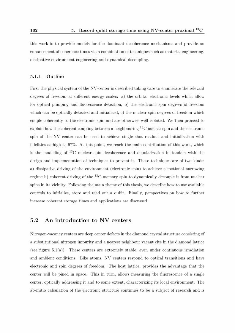
102 5. Record qubit storage time using NV-center proximal 13C
this work is to provide models for the dominant decoherence mechanisms and provide an
enhancement of coherence times via a combination of techniques such as material engineering,
dissipative environment engineering and dynamical decoupling.
5.1.1 Outline
First the physical system of the NV-center is described taking care to enumerate the relevant
degrees of freedom at different energy scales: a) the orbital electronic levels which allow
for optical pumping and fluorescence detection, b) the electronic spin degrees of freedom
which can be optically detected and initialized, c) the nuclear spin degrees of freedom which
couple coherently to the electronic spin and are otherwise well isolated. We then proceed to
explain how the coherent coupling between a neighbouring 13C nuclear spin and the electronic
spin of the NV center can be used to achieve single shot readout and initialization with
fidelities as high as 97%. At this point, we reach the main contribution of this work, which
is the modelling of 13C nuclear spin decoherence and depolarization in tandem with the
design and implementation of techniques to prevent it. These techniques are of two kinds:
a) dissipative driving of the environment (electronic spin) to achieve a motional narrowing
regime b) coherent driving of the 13C memory spin to dynamically decouple it from nuclear
spins in its vicinity. Following the main theme of this thesis, we describe how to use available
controls to initialize, store and read out a qubit. Finally, perspectives on how to further
increase coherent storage times and applications are discussed.
5.2 An introduction to NV centers
Nitrogen-vacancy centers are deep center defects in the diamond crystal structure consisting of
a substitutional nitrogen impurity and a nearest neighbour vacant cite in the diamond lattice
(see figure 5.1(a)). These centers are extremely stable, even under continuous irradiation
and ambient conditions. Like atoms, NV centers respond to optical transitions and have
electronic and spin degrees of freedom. The host lattice, provides the advantage that the
center will be pined in space. This in turn, allows measuring the fluorescence of a single
center, optically addressing it and to some extent, characterizing its local environment. The
ab-initio calculation of the electronic structure continues to be a subject of research and is
5.2 An introduction to NV centers 103
beyond the scope of this thesis [43, 42]. The widely accepted energy structure for these centers
is presented here in a phenomenological way.
(a) NV-center real-space layout (b) NV-center energy levels
Figure 5.1: a) An NV-center is obtained by removing two nearest neighbour carbons in
the diamond lattice and replacing one of them by a nitrogen atom (light grey) while keeping
the lattice location vacant (blue). In practice, a way to fabricate these centers is via high
temperature annealing of natural or implanted nitrogen impurities until they become attached
to a vacancy. b) Schematic level diagram for an NV center (left box) and a 13C nuclear spin
(right box) under illumination with green laser light. The green arrows indicate optical
transitions addressed by our green laser pulse, red arrows show electronic decay and blue
arrows indicate depolarization of the electronic spin. The transition rates for NV are taken
from [88] with the decay rate from the electronic excited state to the ground state γ = 113ns ,
the decay rate from the singlet to ms = 0 of the electronic ground state Γ = 1300ns and the
decay rate from the electronic excited states with ms = ±1 to the singlet γb = 0.3γ. Moreover
we assumed the decay rate of the excited state of NV0 to be on the same order as for NV. The
deionization rate from NV to NV0 is taken to be γ1 = I/Isat70ns and the ionization rate γ2 = 2γ1
[126]. The depolarization time for the electronic spin for NV is taken to be TNV−
1e = 8ms
and for the case of NV0, TNV0
1e = 6µs [126]. All the remaining rates are taken to be zero.
Reprinted from Science 336 (2012) 1283-1286 with permission from AAAS.

104 5. Record qubit storage time using NV-center proximal 13C
5.2.1 Electronic energy levels
Two possible charge states have been found to be long lived for NV centers, a neutral state
NV0 and a singly charged state NV−. Each of these charge states can be electronically excited
with respective zero-phonon lines of 2.16eV (575nm) for NV0 and 1.945eV (637nm) for NV−.
Compare this to a band gap of 5.5eV for diamond. There are 6 electrons contributing to
the electronic structure of the NV−, one valence electron for each of the nearest neighbour
carbons of the vacancy, two from the substitutional nitrogen and an extra negative charge.
The nitrogen and the vacancy partially break the symmetries of the diamond lattice leaving
only a C3V symmetry around the axis they define (see figure 5.1(a)). The NV− is most
abundant in nautral diamond, and will also play a dominant role in this work. However, the
NV− can become deionized by optical irradiation so NV0 should not be dismissed completely.
The orbital ground state of NV− transforms as A1 (i.e. is invariant) under C3V symmetry
transformations. There are two dipole allowed excited states at 1.945eV with E character
which can be optically excited and fluoresce. By employing a Hanbury Brown and Twiss
type setup to collect NV-center fluorescence, it is possible to ascertain that a single center is
being detected[78]. Typically, excitation and fluorescence processes occur primarily through
the phonon sidebands (630–800nm), with the excited states showing a radiative lifetime of
≈13ns. However, there is also a slower non radiative decay channel for the excited states via
a shelf state which is responsible for polarizing the electronic spin.
While the NV− energy structure is relatively well understood, knowledge of NV0 states
and dynamics have not reached the same degree of maturity and consensus. In our study, we
consider a simple model for the NV0 in which only a doublet ground state and exited state
are involved [126]. However, there are a few reasons why our results do not show a strong
dependence on the detailed description of NV0. The main one, is that all of the coherent
manipulation of our system occurs exclusively in the NV− states. Furthermore, it is expected
that at the relevant filling conditions, the NV centers spend more than twice as much time in
NV− states than in NV0 states, even during optical irradiation. Finally, the electronic spin
depolarization is more than 1000 times faster for NV0 state than for NV− and experiments
suggest that NV0 states have no orbital angular momentum. This leads us to expect that the
weak hyperfine interaction with distant 13C can be neglected due to motional averaging.

5.2 An introduction to NV centers 105
5.2.2 Electronic spin sublevels
Both the ground orbital state and the discussed excited states of NV− have an additional
triplet spin structure which is mainly preserved by optical transitions. Electronic spin-spin
interactions provide a zero-field splitting (ZFS) described by ∆gs/esS2z . In the long lived
electronic ground state ∆gs ≈ 2.87GHz allows microwave (MW) driving of electronic transi-
tions. For the excited states, the ZFS is approximately half as strong ∆es ≈ 1.43GHz [96].
However, due to the short lifetime of excited orbital states coherent control is more reliable
in the ground state. Additionally, the energy levels of electronic spin states are shifted by
an external magnetic field B which in our setup will be fixed along the NV symmetry axis.
Microwave pulses can coherently drive transitions among these electronic states. The feature
which makes NV center electronic spins most attractive, is their optical polarizability (into
ms = 0 state) and the possibility of optical measurement via spin dependent fluorescence.
5.2.3 Nuclear spin environment
At longer time scales, nuclear spins, which interact with the electronic spin degree of freedom
via hyperfine interaction begin to play a relevant role in NV-center dynamics. The Nitrogen
atom of the NV-center provides a nuclear spin which is universally present, either the naturally
occurring 14N with (I = 1) or its less likely (0.4%) stable isotope 15N with (I = 1/2) which
may also be selectively implanted. Due to its universality, many proposals have been made
involving the nitrogen nuclear spin[116], however, its strong coupling with the NV electronic
spin rule out prolonged coherent storage. Due to the strong electronic ZFS, and the symmetric
placement of the nitrogen the ANzzINz Sz is the only remaining term of the hyperfine interaction
in the electronic ground space, with ANzz ≈ −2.16MHz. The nitrogen nuclear spin also present
a zero field splitting given by P (INz )2, with P ≈ −5MHz.
While most carbon atoms (12C) in the diamond lattice have no nuclear spins the remaining
13C nuclear spins (I = 1/2) provide a bath with which the electronic NV-spin may interact.
In particular, the hyperfine interaction of the electronic spin with nearest neighbour 13C, is
even greater than with the 14N nuclear spin. From first principles, the hyperfine interaction
106 5. Record qubit storage time using NV-center proximal 13C
of the electronic spin with a 13C nuclear spins is given by
Hhf =− γeγ13C2µ0π~2|ψe(r = 0)|2
3S · I13C
+~2µ0γeγ13C
4π
⟨1
r3
(S · I13C − 3(n · S)(n · I13C)
)⟩,
(5.1)
where γe and γ13C are the gyromagnetic moments of the electron and the 13C nuclear spin
respectively, r and n are the magnitude and direction of the position r of the electron respect to
the nuclear spin and the brackets denote expectation value with respect to the electronic wave
function ψe(r) (taking coordinate origin at the nuclear spin). The first term corresponds to a
Fermi contact interaction whereas the second corresponds to the usual magnetic dipole-dipole
interaction. In the case of the NV-center, the electronic wave function actually corresponds to
six valence electrons. In practice, the hyperfine interaction can be represented by an orbital
state dependent hyperfine tensor
Hhf =∑
µ,ν∈{x,y,z}
SµAµ,νIν . (5.2)
For proximal nuclear spins, this tensor can be obtained experimentally and/or from first prin-
ciple electronic wave function calculations. For distant nuclear spins, the contact interaction
decays exponentially and can be discarded, and a point-dipole approximation which places
all electronic density at the NV is justified for estimating the hyperfine tensor[97].
In addition to the interaction with the electronic spin, each nuclear spin interacts directly
with the external magnetic field Hb = γ13C~B · I. Finally, relatively weak magnetic dipole-
dipole interactions exists among the nuclear spins
Hdd =∑j<k
−µ0
4π
γjγk~2
rjk3(3(Ij · njk)(Ik · njk)− Ij · Ik) , (5.3)
where j, k index over the different nuclear spins and the vector rjk with length rjk and
orientation njk is the relative position of the two nuclear spins.
The stable 13C isotope occurs with a natural abundance of 1.1%, whereas material engi-
neering may reduce this ratio to as low as 0.01%. This reduction is a key ingredient to our
approach of using 13C nuclear spins as memories since it effectively reduces the dipole-dipole
coupling among neighbouring 13C and the typical hyperfine interaction with the NV elec-
tronic spin. This second effect allows reaching the motional narrowing regime in which the
electronic spin is driven faster than the hyperfine interaction time.
5.3 Qubit initialization and readout 107
The effective surrounding 13C concentration determines the coherence time of the elec-
tronic spin as having a time scale similar to the hyperfine coupling[14]. Thus, in order to
have some degree of coherent coupling between the NV electronic spin and a 13C, the closest
nuclear spin should be significantly closer than the others. In the case of the experiment
conducted the nearest 13C spin addressed was at a distance of 1.7nm. Given the sample 13C
to 12C concentration of 10−4, approximately 7% of the NV-centers have such a proximal 13C.
Thus, significant search needs to be conducted in order to locate an NV presenting a single
13C with such a strong hyperfine interaction which can be clearly singled out from the rest of
the nuclear spin environment. Alternatively it may be possible to improve on existing tech-
niques to place single 13C nuclear spins close to an NV-center [115] such that sample quality
is not compromised.
5.3 Qubit initialization and readout
Relatively long coherence times have been demonstrated in bulk electron spin resonance
(ESR) and nuclear magnetic resonance (NMR) experiments [79, 13, 121]. A shortfall of
theses systems is that single spin initialization and readout are quite challenging and only
global addressing can be used. In contrast, one of the attractive qualities of NV-centers is the
possibility of optically inducing spin polarization and optically detected magnetic resonance.
Due to diffraction limits, the optically achievable spatial resolution ≈200nm is orders of
magnitude higher than what is achievable with microwave or radio-frequency allowing to
resolve single NV centers at sufficiently low density. A second advantage is the large optically
achievable spin polarizations (90% for the electronic spin [36] or even 98% for isotopic 15N
nuclear spins [62]) which are unachievable by thermal equilibration in standard NMR or ESR
experiments. Furthermore, the single spin repetitive readout techniques that will be discussed
allow achieving an even higher degree of polarization on neighbouring 13C nuclear spins.
In this section we will describe 13C initialization and single shot readout following the work
by Neumann et al. [95] (see figure 5.3). The main ingredients of this approach are a) optical
readout and initialization of electronic spin b) CnNOTe logic gate which flips the electronic
spin conditioned on the 13C nuclear spin c) arbitrary gates acting on the 13C nuclear spin.
Finally, we may infer the nuclear state and our uncertainty of it from the photon counting
statistics which is obtained. We will describe these steps one by one in what follow and finally
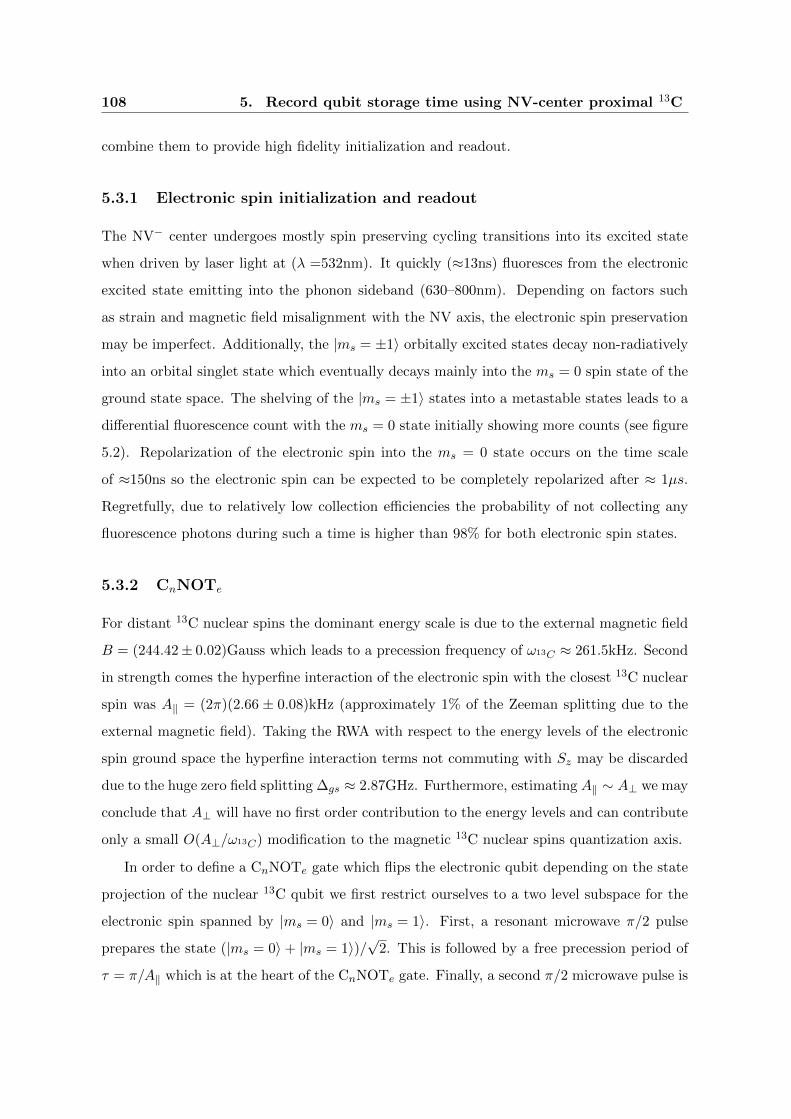
108 5. Record qubit storage time using NV-center proximal 13C
combine them to provide high fidelity initialization and readout.
5.3.1 Electronic spin initialization and readout
The NV− center undergoes mostly spin preserving cycling transitions into its excited state
when driven by laser light at (λ =532nm). It quickly (≈13ns) fluoresces from the electronic
excited state emitting into the phonon sideband (630–800nm). Depending on factors such
as strain and magnetic field misalignment with the NV axis, the electronic spin preservation
may be imperfect. Additionally, the |ms = ±1〉 orbitally excited states decay non-radiatively
into an orbital singlet state which eventually decays mainly into the ms = 0 spin state of the
ground state space. The shelving of the |ms = ±1〉 states into a metastable states leads to a
differential fluorescence count with the ms = 0 state initially showing more counts (see figure
5.2). Repolarization of the electronic spin into the ms = 0 state occurs on the time scale
of ≈150ns so the electronic spin can be expected to be completely repolarized after ≈ 1µs.
Regretfully, due to relatively low collection efficiencies the probability of not collecting any
fluorescence photons during such a time is higher than 98% for both electronic spin states.
5.3.2 CnNOTe
For distant 13C nuclear spins the dominant energy scale is due to the external magnetic field
B = (244.42± 0.02)Gauss which leads to a precession frequency of ω13C ≈ 261.5kHz. Second
in strength comes the hyperfine interaction of the electronic spin with the closest 13C nuclear
spin was A‖ = (2π)(2.66 ± 0.08)kHz (approximately 1% of the Zeeman splitting due to the
external magnetic field). Taking the RWA with respect to the energy levels of the electronic
spin ground space the hyperfine interaction terms not commuting with Sz may be discarded
due to the huge zero field splitting ∆gs ≈ 2.87GHz. Furthermore, estimating A‖ ∼ A⊥ we may
conclude that A⊥ will have no first order contribution to the energy levels and can contribute
only a small O(A⊥/ω13C) modification to the magnetic 13C nuclear spins quantization axis.
In order to define a CnNOTe gate which flips the electronic qubit depending on the state
projection of the nuclear 13C qubit we first restrict ourselves to a two level subspace for the
electronic spin spanned by |ms = 0〉 and |ms = 1〉. First, a resonant microwave π/2 pulse
prepares the state (|ms = 0〉+ |ms = 1〉)/√
2. This is followed by a free precession period of
τ = π/A‖ which is at the heart of the CnNOTe gate. Finally, a second π/2 microwave pulse is
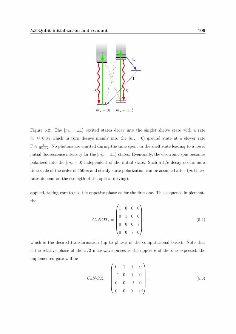
5.3 Qubit initialization and readout 109
| ms = 0i | ms = ±1i
�
�b
� �
Figure 5.2: The |ms = ±1〉 excited states decay into the singlet shelve state with a rate
γb ≈ 0.3γ which in turn decays mainly into the |ms = 0〉 ground state at a slower rate
Γ ≈ 1300ns . No photons are emitted during the time spent in the shelf state leading to a lower
initial fluorescence intensity for the |ms = ±1〉 states. Eventually, the electronic spin becomes
polarized into the |ms = 0〉 independent of the initial state. Such a 1/e decay occurs on a
time scale of the order of 150ns and steady state polarization can be assumed after 1µs (these
rates depend on the strength of the optical driving).
applied, taking care to use the opposite phase as for the first one. This sequence implements
the
CnNOTe =
1 0 0 0
0 1 0 0
0 0 0 i
0 0 i 0
(5.4)
which is the desired transformation (up to phases in the computational basis). Note that
if the relative phase of the π/2 microwave pulses is the opposite of the one expected, the
implemented gate will be
CnNOTe =
0 1 0 0
−1 0 0 0
0 0 −i 0
0 0 0 +i
, (5.5)

110 5. Record qubit storage time using NV-center proximal 13C
which is also acceptable up to phases in the computational basis and a swap in the definition
of the computational basis states for the 13C nuclear spin. It is experimentally challenging
to control the MW frequency such that it does not drift from the electronic resonance fre-
quency over a period τ . A frequency mismatch δ such that δτ = ±π/2 would already erase
all measurable contrast. This requires the resonance frequency to be matched within 1kHz.
Such drifts may be induced by temperature since the ZFS ∆gs has been reported to show a
temperature dependence of around (2π)74kHzK imposing a thermal stability of 0.02K. This is
experimentally challenging, and is avoided by defining the nuclear states |↑〉, (|↓)〉 as corre-
sponding to high (low) fluorescence. In the experimental setup considered, such frequency
drifts do occur on the time scale of 30 minutes changing this definition.
The MW pulses manipulating the electronic spin were performed with a Rabi frequency
on the order of (2π)40MHz which is more than 10000 times faster than the hyperfine splitting
and provides pulses which are approximately instantaneous with respect to it. Additionally
the 14N nuclear spin can be assumed to be dynamically polarized to 71% by the optical driving
due to an anti-crossing in the electronic excited state [62].
5.3.3 Nuclear spin gates and preparation of arbitrary states
By repetitively mapping the state of the nuclear spin onto the electronic spin and performing
fluorescence detection, it is possible to determine the state (either |↑〉 or |↓〉) to a very high
precision (purity). A full set of single qubit gates allows us to prepare any known state from
such a known initial state. Using radio-frequency driving with well controlled phases and in
resonance with the ω13C magnetic Zeeman splitting, (261kHz) it is possible to drive coherent
transitions on the 13C nuclear spins. In the considered experimental setup, these transitions
could be driven with Rabi frequencies of ≈ (2π)100kHz.
5.3.4 Repetitive readout and initialization
As mentioned earlier, each time the nuclear spin state is mapped into the electronic spin,
fluorescence counts provide an average of no more than 0.02 photon detections. In addition
to the low photon collection efficiency and imperfect contrast between |ms = 0〉 and |ms = 1〉states, there are other factors which lead to low contrast such as: imperfect initialization of
ms = 0, imperfect CnNOTe gate implementation due to electronic dephasing and unpolarized
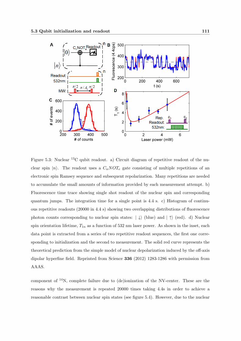
5.3 Qubit initialization and readout 111
Figure 5.3: Nuclear 13C qubit readout. a) Circuit diagram of repetitive readout of the nu-
clear spin |n〉. The readout uses a CnNOTe gate consisting of multiple repetitions of an
electronic spin Ramsey sequence and subsequent repolarization. Many repetitions are needed
to accumulate the small amounts of information provided by each measurement attempt. b)
Fluorescence time trace showing single shot readout of the nuclear spin and corresponding
quantum jumps. The integration time for a single point is 4.4 s. c) Histogram of continu-
ous repetitive readouts (20000 in 4.4 s) showing two overlapping distributions of fluorescence
photon counts corresponding to nuclear spin states: | ↓〉 (blue) and | ↑〉 (red). d) Nuclear
spin orientation lifetime, T1n as a function of 532 nm laser power. As shown in the inset, each
data point is extracted from a series of two repetitive readout sequences, the first one corre-
sponding to initialization and the second to measurement. The solid red curve represents the
theoretical prediction from the simple model of nuclear depolarization induced by the off-axis
dipolar hyperfine field. Reprinted from Science 336 (2012) 1283-1286 with permission from
AAAS.
component of 14N, complete failure due to (de)ionization of the NV-center. These are the
reasons why the measurement is repeated 20000 times taking 4.4s in order to achieve a
reasonable contrast between nuclear spin states (see figure 5.4). However, due to the nuclear

112 5. Record qubit storage time using NV-center proximal 13C
spin depolarization (T1n ≈ 25s during repetitive readout), further increase in the repetition
number provides little improvement for the readout fidelity.
In order to prepare definite nuclear spin states, it is possible to post select measurements
for which the number of photons counts is above/below predefined thresholds. In the case
of the experiment realized these were taken to be 147(195) photon counts during the last
10000 repetitions (2.2s) which leads to an initialization fidelity of ≈ 97%. In the case of
measurement, readout fidelity can be estimated at (91.9 ± 2.5)% from the overlap between
the count distributions associated to the two possible initial states.
Figure 5.4: Photon count statistics and initialization fidelity a) The number of events associ-
ated to a given number of detected photons is plotted in a histogram (blue) after initialization
of the nuclear spin in |↓〉 (green) and |↑〉 (red) and 10000 repetitive readouts (2.2s). The solid
curves correspond to a theoretical fit accounting for the effect of a possible nuclear spin flips
on the ideally Gaussian distributions. The green and red regions indicate photon count num-
bers for which initialization is assumed in the |↓〉 respectively |↑〉 nuclear states. b) The green
and red curves indicate the initialization fidelity of |↓〉 respectively |↑〉 nuclear states as a
function of the count threshold taken. Stricter count thresholds lead to higher fidelity but
to discarding a larger fraction of initializations with the net effect of prolonging the effective
initialization time required. Reprinted from Science 336 (2012) 1283-1286 with permission
from AAAS.

5.4 Nuclear spin coherence and depolarization 113
5.4 Nuclear spin coherence and depolarization
One of the main achievements of this work is to demonstrate a prolonged coherent storage
time afforded by the 13C nuclear spin. In order to do this, we must first understand the
processes that lead to nuclear spin depolarization and dephasing. In the dark (laser turned
off), no decay of the 13C nuclear spin was detected in a time of 200s, so we may assume that
under these conditions, spin flip processes are suppressed on this time scale.
In order to measure the coherence time of the 13C nuclear spin, an NMR Ramsey exper-
iment is performed. After a measurement based initialization, a π/2 RF pulse puts the 13C
nuclear spin in a superposition |↑ + ↓〉 /√
2. Then it is left to freely precess for a variable time
t. A second π/2 RF pulse is applied before a final repetitive readout of the 13C spin. Each
measurement must be repeated many times in order to get to estimate the expectation value
of |↑〉 〈↑|. The detected oscillation of |↑〉 〈↑| decay on a time scale of T ?2n = (8.2 ± 1.3)ms.
The origin of this relatively fast dephasing are electronic spin flips which occur on a longer
time scale than the hyperfine coupling T1e > A−1‖ . Indeed, experimental measurements yield
T1e = (7.5 ± 0.8)ms confirming T1e ≈ T ?2n. The reason for this is that a single flip of the
electronic spin timed at random during a period π/A‖ imprints a completely random phase
on the 13C nuclear spin.
5.4.1 Spin fluctuator model and motional narrowing
The approach we take to reduce dephasing is to continuously drive the electronic spin from
the magnetic states |ms = ±1〉 into non magnetic |ms = 0〉 state. By doing this with a
green laser beam, electronic (de)ionization transitions are also driven at rates γ(2)1 as well
as increasing the effective depolarization time of the electronic spin. A regime analogous to
motional averaging [63] can be achieved when the mixing time of the defined process is faster
than the hyperfine coupling. In this regime, both T1n and T2n increase linearly with the laser
intensity.
In order to qualitatively understand the process of motional narrowing, let us consider
an illustrative simplified scenario with only two possible NV eigenstates∣∣ms = ±1
2
⟩, each
having its own hyperfine interaction with the proximal 13C nuclear spin. We assume that the
NV state is driven incoherently as is the case for the laser driving. Finally, we assume that
transitions among electronic states occur at a rate γ. The nuclear spin Hamiltonian is then
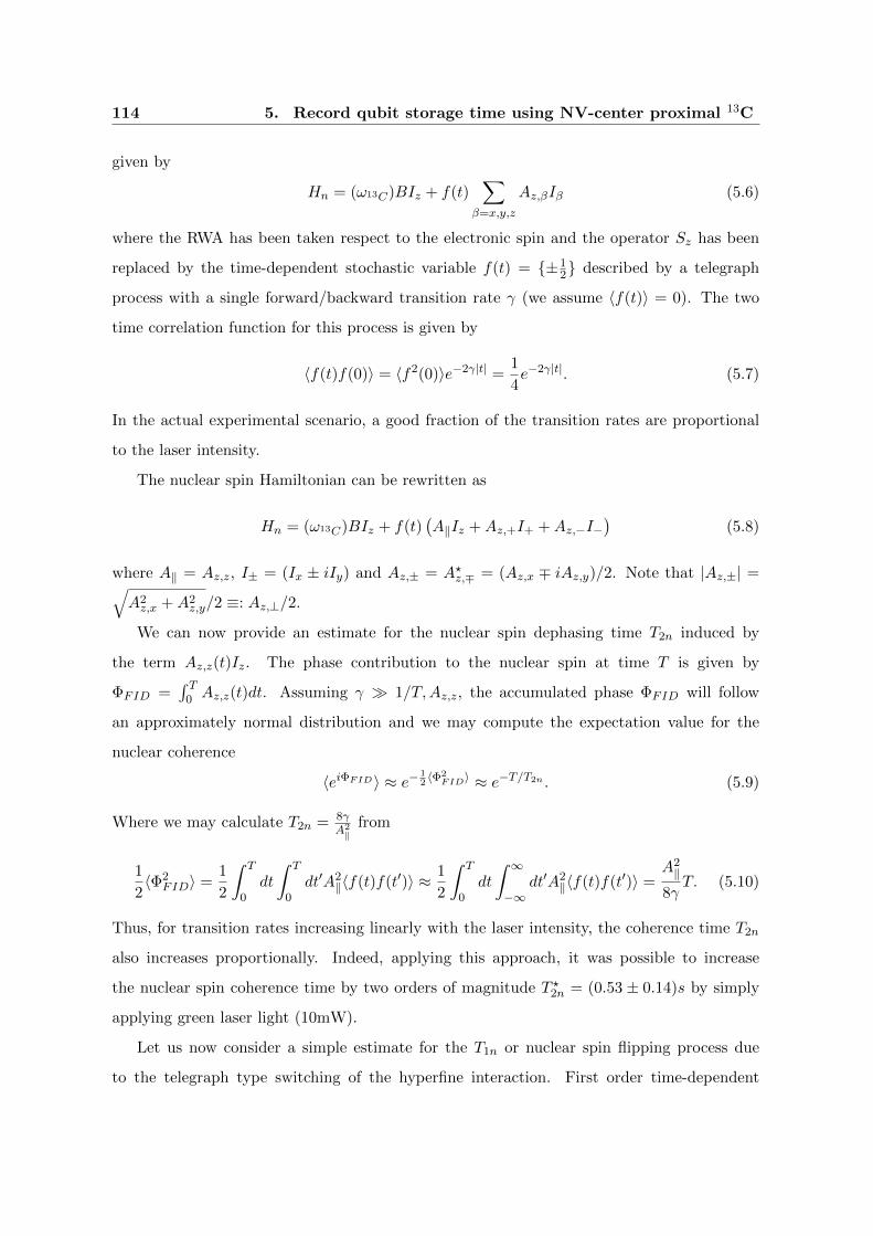
114 5. Record qubit storage time using NV-center proximal 13C
given by
Hn = (ω13C)BIz + f(t)∑
β=x,y,z
Az,βIβ (5.6)
where the RWA has been taken respect to the electronic spin and the operator Sz has been
replaced by the time-dependent stochastic variable f(t) = {±12} described by a telegraph
process with a single forward/backward transition rate γ (we assume 〈f(t)〉 = 0). The two
time correlation function for this process is given by
〈f(t)f(0)〉 = 〈f2(0)〉e−2γ|t| =1
4e−2γ|t|. (5.7)
In the actual experimental scenario, a good fraction of the transition rates are proportional
to the laser intensity.
The nuclear spin Hamiltonian can be rewritten as
Hn = (ω13C)BIz + f(t)(A‖Iz +Az,+I+ +Az,−I−
)(5.8)
where A‖ = Az,z, I± = (Ix ± iIy) and Az,± = A?z,∓ = (Az,x ∓ iAz,y)/2. Note that |Az,±| =√A2z,x +A2
z,y/2 ≡: Az,⊥/2.
We can now provide an estimate for the nuclear spin dephasing time T2n induced by
the term Az,z(t)Iz. The phase contribution to the nuclear spin at time T is given by
ΦFID =∫ T
0 Az,z(t)dt. Assuming γ � 1/T,Az,z, the accumulated phase ΦFID will follow
an approximately normal distribution and we may compute the expectation value for the
nuclear coherence
〈eiΦFID〉 ≈ e− 12〈Φ2FID〉 ≈ e−T/T2n . (5.9)
Where we may calculate T2n = 8γA2‖
from
1
2〈Φ2
FID〉 =1
2
∫ T
0dt
∫ T
0dt′A2
‖〈f(t)f(t′)〉 ≈ 1
2
∫ T
0dt
∫ ∞−∞
dt′A2‖〈f(t)f(t′)〉 =
A2‖
8γT. (5.10)
Thus, for transition rates increasing linearly with the laser intensity, the coherence time T2n
also increases proportionally. Indeed, applying this approach, it was possible to increase
the nuclear spin coherence time by two orders of magnitude T ?2n = (0.53 ± 0.14)s by simply
applying green laser light (10mW).
Let us now consider a simple estimate for the T1n or nuclear spin flipping process due
to the telegraph type switching of the hyperfine interaction. First order time-dependent

5.4 Nuclear spin coherence and depolarization 115
perturbation theory provides an estimate for the transition rates in both directions (lowering
and raising), given by
Γ↑ =
(A⊥2
)2
Sq(−γ13CB) and Γ↓ =
(A⊥2
)2
Sq(γ13CB). (5.11)
where Sq(ω) is defined as
Sq(ω) =
∫ ∞−∞
dτeiωτ 〈f(τ)f(0)〉 (5.12)
and according to eq. (5.7) can be calculated to be Sq(γ13CB) = γ4γ2+(γ13CB)2 . This leads to
the transition rates,
1/T1n,opt = Γ↓ + Γ↑ =A2⊥
8
γ
γ2 + (ω13CB/2)2(5.13)
In the dark, the nuclear spin lifetime is no longer limited by the optically induced depo-
larization (note that the numerator in eq. (5.13) vanishes but the denominator does not).
In this context resonant dipole-dipole interactions among 13C nuclear spins may provide a
significant contribution. The dipole-dipole interactions take the form
Hdd = Ddd
[3(I · n)(I′ · n)− I · I′
], (5.14)
where I is the memory spin operator and I′ is the spin operator for a neighbouring 13C nuclear
spin and n is a unit vector oriented in the direction connecting the two nuclei. At the present
13C concentration, the Ddd can be expected to be of the order of 1Hz. Since we do not
know the precise direction of n with respect to the static magnetic field we shall assume an
intensity of approximately Ddd for each of the components. This is much smaller than the
Zeeman splitting of the nuclear spins due to the external magnetic field B and even smaller
than the dephasing rate at experimentally addressed laser intensity. Consider a simplified
model in which there is a single neighbouring 13C nuclear spin. The electronic spin spends
approximately 1/3 of the time in the |ms = 0〉 state, the only state which is expected to allow
resonant I−I′+ + I+I
′− transitions from the dipole-dipole interaction. The permanence time
of the electronic spin in the |ms = 0〉 state is exponentially distributed with parameter 1/T1e.
The flip-flop probability per visit to |ms = 0〉 may be estimated by
1
T1e
∫ ∞0
e−t/T1e sin2(Dddt)dt =D2dd
2T−21e + 2D2
dd
, (5.15)
whereas the rate of visits to the |ms = 0〉 state is half the depolarization rate 12T1e
. For
T1eA‖ � 1, the phase of the memory spin is lost on each |ms = ±1〉 visit and thus, spin flips
116 5. Record qubit storage time using NV-center proximal 13C
accumulate incoherently with
T1n,dd ≈ 2T−1
1e +D2ddT1e
D2dd
≈ 2
D2ddT1e
. (5.16)
In practice, no significant depolarization was measured for the nuclear spin in a time scale of
200s, which is consistent with the long T1n,dd predicted by this last equation.
We may also analyse the dipole-dipole contribution to the memory flip rate in the motional
narrowing regime of T1eA‖ � 1. In this regime, we may start from a coarse grained time
dynamics with respect to T1e for the 13C memory spin where the effect of the electronic spin
are already included as a dissipative dephasing of rate T−12n . This is valid since the time scale
of the perturbation considered, nuclear dipole-dipole coupling, is expected to be of the order
of 1 second and hence much longer than the necessary time coarse graining. We now consider
the flip-flop between the memory spin and a neighbouring nuclear spin Ddd(I+I′− + I−I
′+).
We may now take a time dependent perturbative expansion (now of a Liouvillian) in order
to extract the effective flip-flop rates, which we identify with T−11n,dd. We expand
Γ↑↓→↓↑t ≈ 〈↓↑| e(L0+Hdd)t(|↑↓〉 〈↑↓|) |↓↑〉 (5.17)
to first non vanishing (second) order in Ddd, where L0 includes the possibly different Zee-
man splitting of the two nuclear spins and the dephasing of the memory spin whereas
Hdd(ρ) = [Ddd(I+I′+I−I
′+), ρ]. After some relatively straightforward calculations and stan-
dard approximations we arrive at
T−11n,dd ≈ Γ↑↓→↓↑ ≈ 2
D2ddT
−12n
T−22n + ∆2
ω
(5.18)
where T2n is the effective dephasing time of the memory spin and ∆ω is the effective energy
detuning between the two nuclear spins (i.e. the difference between individual effective Zee-
man splitting possibly due to the presence of an effective field from the electronic spin or
magnetic field gradient). Note that homogeneous variations in the external magnetic field do
not contribute to the dephasing or energy detuning ∆ω, since they would act equally on both
nuclear spins.
This term may be ineffective on the memory spin due to a possibly large ∆ω or effective
dephasing rate T−12n . However, this same analysis applies for any pair of 13C spins in the
neighbourhood of memory nucleus. In turn, flipping of neighbouring 13C nuclear spins can
5.4 Nuclear spin coherence and depolarization 117
produce dephasing of the memory spin due to a change in the effective magnetic field they
produce.
As evinced by the term ∆2ω in the denominator of eq. (5.18), it is possible that the
nuclear spin flip-flop processes to be frozen by energy detuning. However, the nuclear IzI′z
term of the nuclear dipole-dipole interactions will imprint a phase on the memory spin which is
dependent on the environment state. Note that during coherence measurement experiments,
the π/2 initialization RF pulse (as all RF pulses) acts globally on the 13C nuclear spins and
removes any hope of having a preferred basis for the states. The accumulated phase may
not be reverted by applying a radio-frequency echo π pulses since these pulses flip both the
memory spin and the environment leading to a continued accumulation of phase instead of a
cancellation. This leads to the need of decoupling homo-nuclear dipole-dipole interactions.
5.4.2 Decoupling of homo-nuclear dipole-dipole interactions
As mentioned, the dipole-dipole interaction among 13C nuclear spins starts playing a relevant
role once one attempts to reach coherence times of the order of 1s. It is here that RF
decoupling pulse sequences can be of use. Decoupling pulse sequences have been extensively
studied in NMR where most of them have been introduced in order to study different aspect
of nuclear spin dynamics [123]. The pulse sequence that was experimentally used was derived
from MREV-8, which in turn is derived from a four pulse sequence named WaHuHa, after
Waungh, Huber and Haberlen designed to decouple homonuclear dipole-dipole interaction[91].
One of the fruitful approaches to analyse these sequences is to use the average Hamiltonian
theory. Here, the effect of the pulses are studied by moving into an interaction picture,
a toggling frame with respect to the applied RF pulses. Provided that the characteristic
frequencies ω of the natural Hamiltonian H satisfy ωt� 1, where t is the time during which
the Hamiltonian evolves between pulses and that the pulse time τp is negligible, a Magnus
expansion may be performed to describe the effective Hamiltonian Heff . The effective Heff
is defined such that the effective evolution of the system at times nt is given by U(nt) =
exp(−intHeff ) for integer values of n. The Magnus expansion gives a systematic series
development of Heff as
Heff = H(0) +H(1) +H(2) + . . . . (5.19)
Assuming the piecewise constant interaction Hamiltonians Hj =∏jl=1 U
−1l H
∏1l=j Ul corre-
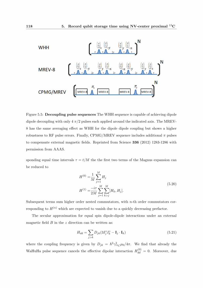
118 5. Record qubit storage time using NV-center proximal 13C
Figure 5.5: Decoupling pulse sequences The WHH sequence is capable of achieving dipole
dipole decoupling with only 4 π/2 pulses each applied around the indicated axis. The MREV-
8 has the same averaging effect as WHH for the dipole dipole coupling but shows a higher
robustness to RF pulse errors. Finally, CPMG/MREV sequence includes additional π pulses
to compensate external magnetic fields. Reprinted from Science 336 (2012) 1283-1286 with
permission from AAAS.
sponding equal time intervals τ = t/M the the first two terms of the Magnus expansion can
be reduced to
H(0) =1
M
M∑j=1
Hj
H(1) =−iτ2M
M∑j=1
M∑k>j
[Hk, Hj ].
(5.20)
Subsequent terms sum higher order nested commutators, with n-th order commutators cor-
responding to H(n) which are expected to vanish due to a quickly decreasing prefactor.
The secular approximation for equal spin dipole-dipole interactions under an external
magnetic field B in the z direction can be written as:
Hdd =∑j>k
Djk(3Izj I
zk − Ij · Ik) (5.21)
where the coupling frequency is given by Djk = ~2γ213Cµ0/4π. We find that already the
WaHuHa pulse sequence cancels the effective dipolar interaction H(0)dd = 0. Moreover, due
5.5 Conclusions and perspective 119
to the symmetry of the pulse sequence, Uk+1 = U †M−k, all odd order terms of the Magnus
expansion cancel H(2n+1)dd = 0. This leaves the second order term H
(2)dd as the first potentially
non trivial correction. Assuming τ ≈ 0.04s for four repetitions of the CPMG/MREV-8
pulse sequence, in a 2s coherence measurement, and a typical dipole-dipole interaction of
Ddd ≈ 1Hz the prefactor for the leading correction is (Dddτ)2Ddd ≈ 10−3Hz which would not
be detectable in coherence measures of a few seconds.
Combined detuning and dipolar
At high laser power, the ionization induced decoherence is suppressed by motional averag-
ing. As discussed, the CPMG/MREV-8 RF pulse sequence can suppress the dipole-dipole
interaction among nuclear spins up to second order in Dddτ . Furthermore, the sequence can
also suppress, to all orders, the effect of finite detuning δIz of the RF driving with respect
to the actual Zeeman splitting of the nuclear spins which can be of the order of (2π)10Hz.
However, the pulse sequence is not designed to suppress the combined effect of dephasing and
dipolar interactions. Accordingly, the Magnus expansion can no longer be truncated to low
order. In particular, terms of the form (δτ)nD contribute to the expansion and the effective
decoherence time is set by the value of τ for which δτ ≈ 1. This time can be estimated
numerically yielding T2 ≈ 2s (see figure 5.6),in good agreement with experiments. Thus, the
dominant source of decoherence becomes the imperfect tuning of the RF driving used for the
pulse sequence.
5.5 Conclusions and perspective
In this chapter we have presented a physical model for readout, initialization and storage of
a 13C spin proximal to an NV-center. The main contribution of the work comes in the form
of characterization of decoherence and demonstration of decoherence avoiding mechanisms
for a proximal 13C nuclear spin. For (de)ionization rates γ much larger than the hyperfine
interaction, the dephasing rate depends on the parallel component of the dipole field, 1/T ∗2n =
Γopt + Γdd, where Γdd is the spin-bath induced dephasing rate and Γopt ∼A2‖γ is the optically
induced decoherence. The dashed red line in figure 5.7(b) demonstrates that this model is in
good agreement with our data. Application of our decoupling sequence CPMG/MREV-8 (see

120 5. Record qubit storage time using NV-center proximal 13C
Figure 5.6: Combined dephasing from detuning and dipole-dipole interactions
The unitary evolution of a system consisting of a memory 13C nuclear spin and 5 bath spins
was numerically calculated following a CPMG/MREV-8 (with δ = (2π)10Hz driving detuning.
The bath nuclear spins were randomly distributed according to a 0.01% 13C concentration in
the diamond lattice and averaged over 50 realizations. The average predicted coherence shows
a significant decay after 2s. Reprinted from Science 336 (2012) 1283-1286 with permission
from AAAS.
figure 5.7(a)) also allows us to suppress nuclear-nuclear dephasing. We find that the main
imperfection in this decoupling procedure originates from a finite RF detuning. Accounting
for this imperfection, we find excellent agreement with our data, as shown by the dashed blue
line in figure 5.7(b). Moreover, this model indicates that the coherence time increases almost
linearly as a function of applied laser intensity, suggesting a large potential for improvement.
The use of even higher laser intensities is limited by heating of the diamond sample, which
causes drifts in the ESR transition [2]. However, this can be overcome via a combination of
temperature control and careful transition-frequency tracking, yielding an order of magnitude
improvement in the coherence time to approximately one minute. Further improvement can
be achieved by decreasing the hyperfine and the dipole-dipole interaction strength through a
reduction of the 13C concentration, potentially resulting in hour-long storage times. Finally,
it is possible to use coherent decoupling sequences and techniques based upon optimal control
theory [71], which scale more favorably than our current dissipation-based method. With
such techniques, we estimate that the memory lifetime can approach the timescale of phonon-
induced nuclear depolarization, measured to exceed Tmax1n ∼ 36 h [117].
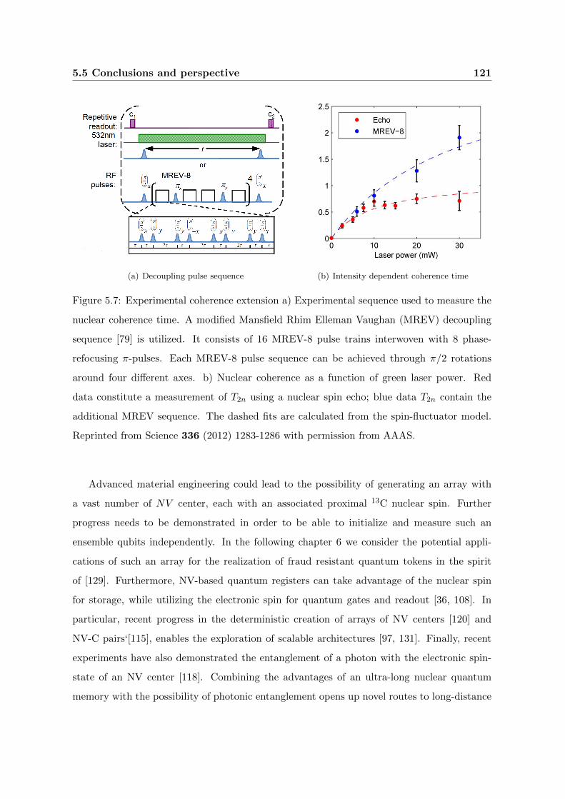
5.5 Conclusions and perspective 121
(a) Decoupling pulse sequence (b) Intensity dependent coherence time
Figure 5.7: Experimental coherence extension a) Experimental sequence used to measure the
nuclear coherence time. A modified Mansfield Rhim Elleman Vaughan (MREV) decoupling
sequence [79] is utilized. It consists of 16 MREV-8 pulse trains interwoven with 8 phase-
refocusing π-pulses. Each MREV-8 pulse sequence can be achieved through π/2 rotations
around four different axes. b) Nuclear coherence as a function of green laser power. Red
data constitute a measurement of T2n using a nuclear spin echo; blue data T2n contain the
additional MREV sequence. The dashed fits are calculated from the spin-fluctuator model.
Reprinted from Science 336 (2012) 1283-1286 with permission from AAAS.
Advanced material engineering could lead to the possibility of generating an array with
a vast number of NV center, each with an associated proximal 13C nuclear spin. Further
progress needs to be demonstrated in order to be able to initialize and measure such an
ensemble qubits independently. In the following chapter 6 we consider the potential appli-
cations of such an array for the realization of fraud resistant quantum tokens in the spirit
of [129]. Furthermore, NV-based quantum registers can take advantage of the nuclear spin
for storage, while utilizing the electronic spin for quantum gates and readout [36, 108]. In
particular, recent progress in the deterministic creation of arrays of NV centers [120] and
NV-C pairs‘[115], enables the exploration of scalable architectures [97, 131]. Finally, recent
experiments have also demonstrated the entanglement of a photon with the electronic spin-
state of an NV center [118]. Combining the advantages of an ultra-long nuclear quantum
memory with the possibility of photonic entanglement opens up novel routes to long-distance
122 5. Record qubit storage time using NV-center proximal 13C
quantum communication and solid state quantum repeaters [35].
Chapter 6
Unforgeable noise-tolerant quantum
tokens
The realization of devices which harness the laws of quantum mechanics repre-
sents an exciting challenge at the interface of modern technology and fundamental
science. An exemplary paragon of the power of such quantum primitives is the
concept of “quantum money” [129]. A dishonest holder of a quantum bank-note
will invariably fail in any counterfeiting attempts; indeed, under assumptions of
ideal measurements and decoherence-free memories such security is guaranteed
by the no-cloning theorem. In any practical situation, however, noise, decoher-
ence and operational imperfections abound. Thus, the development of secure
“quantum money”-type primitives capable of tolerating realistic infidelities is of
both practical and fundamental importance. Here, we propose a novel class of
such protocols and demonstrate their tolerance to noise; moreover, we prove their
rigorous security by determining tight fidelity thresholds. Our proposed proto-
cols require only the ability to prepare, store and measure single qubit quantum
memories, making their experimental realization accessible with current tech-
nologies.
124 6. Unforgeable noise-tolerant quantum tokens
6.1 Introduction
Recent extensions to Wiesner’s original “quantum money” protocol [129] have garnered sig-
nificant interest [1, 86, 94, 38, 39, 85]. One particular extension enables the authentication of
quantum tokens via classical public communication with a trusted verifier [44]. However, to
tolerate noise, the verification process must condone a certain finite fraction of qubit failures;
naturally, such a relaxation of the verification process enhances the ability for a dishonest
user to forge quantum tokens. It is exactly this interplay which we, here, seek to address,
by focusing on a class of ”quantum token”-protocols which involve either direct physical or
classical communication verification of qubit memories.
6.2 Qticket
Our approach to quantum tokens extends the original quantum money primitive[129] by
ensuring tolerance to finite errors associated with encoding, storage and decoding of individual
qubits. We denote the tokens within our first primitive as quantum tickets (qtickets); each
qticket is issued by the mint and consists of a unique serial number and N component quantum
states, ρ =⊗
i ρi, where each ρi is drawn uniformly at random from the set, Q = {|+〉, |−〉, |+i〉, | − i〉, |0〉, |1〉}, of polarization eigenstates of the Pauli spin operators. The mint secretly
stores a classical description of ρ, distributed only among trusted verifiers. In order to redeem
a qticket, the holder physically deposits it with a trusted verifier, who measures the qubits in
the relevant basis. This verifier then requires a minimum fraction, Ftol, of correct outcomes
in order to authenticate the qticket; following validation, the only information returned by
the verifier is whether the qticket has been accepted or rejected.
The soundness of a qticket, e.g. the probability that an honest user is successfully verified,
depends crucially on the experimental fidelities associated with single qubit encoding, storage
and decoding. Thus, for a given qubit ρi, we define the map, Mi, which characterizes the
overall fidelity, beginning with the mint’s encoding and ending with the verifier’s validation;
the average channel fidelity[98] is then given by, Fi = 1/|Q|∑ρitr[ρiMi(ρi)]. With this
definition, the verification probability of an honest user is,
ph =1
|Q|∑ρ∈Q
tr[PaccM(ρ)] ≥ 1− e−ND(Fexp‖Ftol), (6.1)

6.3 Cv-qticket 125
where Q = Q⊗N , Pacc represents the projector onto the subspace of valid qtickets, M =⊗iMi, Fexp = 1/N
∑i Fi is the per qubit average experimental fidelity, and the relative
entropy D is a measure of distinguishability between two binary probability distributions.
Crucially, so long as the average experimental fidelity associated with single qubit processes
is greater than the tolerance fidelity, an honest user is exponentially likely to be verified.
To determine a tight security threshold, we consider the counterfeiting of a single qticket.
For a given tolerance fidelity (Ftol) set by the verifiers, a qticket is only accepted if at least
FtolN qubits are validated. In the event that a dishonest user attempts to generate two
qtickets from a single valid original, each must contain a minimum of FtolN valid qubits to
be authenticated. As depicted in Fig. 1a., in order for each counterfeit qticket to contain
FtolN valid qubits, a minimum of (2Ftol−1)N qubits must have been perfectly cloned. Thus,
for a set tolerance fidelity, in order for a dishonest user to succeed, he or she must be able
to emulate a qubit cloning fidelity of at least 2Ftol − 1. Crucially, so long as this fidelity is
above that achievable for optimal qubit cloning (2/3) [128], a dishonest user is exponentially
unlikely to succeed,
pd =1
|Q|∑ρ∈Q
tr[P⊗2
accT (ρ)]≤ e−ND(2Ftol−1‖2/3), (6.2)
where T represents any completely positive trace preserving (CPTP) qticket counterfeiting
map. To ensure 2Ftol−1 > 2/3, the tolerance fidelity must be greater than 5/6, which is pre-
cisely the average fidelity of copies produced by an optimal qubit cloning map [128]. In certain
cases, an adversary may be able to sequentially engage in multiple verification rounds; how-
ever, the probability of successfully validating counterfeited qtickets grows at most quadrat-
ically in the number of such rounds, and hence, the likelihood of successful counterfeiting
can remain exponentially small even for polynomially large numbers of verifications. Rigor-
ous statement and proofs of these claims are published as supporting information available
online.
6.3 Cv-qticket
Our previous discussion of qtickets assumed that such tokens are physically transferable to
trusted verifiers (e.g. concert tickets); however, in many situations, this assumption of physical
deposition, may either be impossible or undesirable. Recently, it has been shown [44] that it

126 6. Unforgeable noise-tolerant quantum tokens
qticket: ... original
€
ρ1
€
ρ2
€
ρ3
qticket: ... cloned
€
ρ1
€
ρ2
€
ρ3
€
ρN −1
€
ρN
€
ρN −2
€
ρN −1
€
ρN
€
ρN −2€
FtolN
€
FtolNm
inimum
overlap
€
σX€
σZ
“challenge” questions
€
|1〉
€
| 0〉€
|+〉
€
| −〉
a
b
Figure 6.1: a) Depicts the pigeonhole type argument which is utilized in the proof of qticket
soundness. For a tolerance fidelity Ftol, a qticket is only successfully authenticated if it
contains at least FtolN valid qubits. However, for two counterfeit qtickets, not all valid qubits
must coincide. The minimum number of perfectly cloned qubits enabling both qtickets to be
accepted is, (2Ftol − 1)N . b) Depicts the quantum retrieval type situation envisioned for cv-
qtickets. For two verifiers asking complementary “challenge” questions, the optimal strategy
is for the user to measure in an intermediate basis. Such a strategy saturates the tolerance
threshold, F cvtol = 1+1/
√2
2 .

6.3 Cv-qticket 127
remains possible, even remotely, for a holder to prove the validity of a token by responding to
a set of “challenge” questions; these questions can only be successfully answered by measuring
an authentic token. The core behind this approach is to ensure that the “challenge” questions
reveal no additional information about the quantum state of the token.
We now discuss a specific realization of such an approach, the classical verification quan-
tum ticket (cv-qticket), and demonstrate its robustness against noise and operational imper-
fections. In contrast to the case of bare qtickets, a cv-qticket holder will be expected to answer
“challenge” questions and hence to measure qubits himself. Our treatment will contemplate
the possibility of a dishonest holder participating simultaneously in multiple remote verifica-
tions, which could in principle offer the counterfeiter an additional advantage with respect
to the qticket scenario; in particular, certain measurement strategies may yield an increased
likelihood for multiple successful authentications.
One example of a cv-qticket framework, is to utilize a set of eight possible two-qubit
product states with each qubit being prepared as a polarization eigenstate along either X or
Z directions (note that a single qubit framework is also possible):
{|0,+〉, |0,−〉, |1,+〉, |1,−〉, |+, 0〉, |−, 0〉, |+, 1〉, |−, 1〉}.
We then envision each cv-qticket to consist of n blocks, each containing r qubit pairs, and
thus, a total of n × r × 2 qubits; as before, each of the qubit pairs is chosen uniformly at
random from the allowed set above. A “challenge” question consists of requesting the holder
to measure each block (of qubits) along a basis chosen randomly among either X or Z;
naturally, as depicted in Table 1, a valid qubit pair (within a block) is one in which the holder
correctly answers the state for the particular qubit (within the pair) which was prepared along
the questioned basis. For a given tolerance threshold, an overall answer will only be deemed
correct if at least F cvtolr qubits within each of the n blocks are found valid. By analogy to
the qticket case, honest users are exponentially likely to be verified so long as Fexp > F cvtol; in
particular, since there now exist n blocks of qubits, each of which can be thought of as an
individual qticket (with r qubits),
pcvh ≥
(1− e−rD(Fexp‖F cv
tol))n. (6.3)
The proof of cv-qticket security is based upon a generalized formalism of quantum retrieval
games [44, 52], in combination with a generalized Chernoff-Hoeffding bound [61] (details
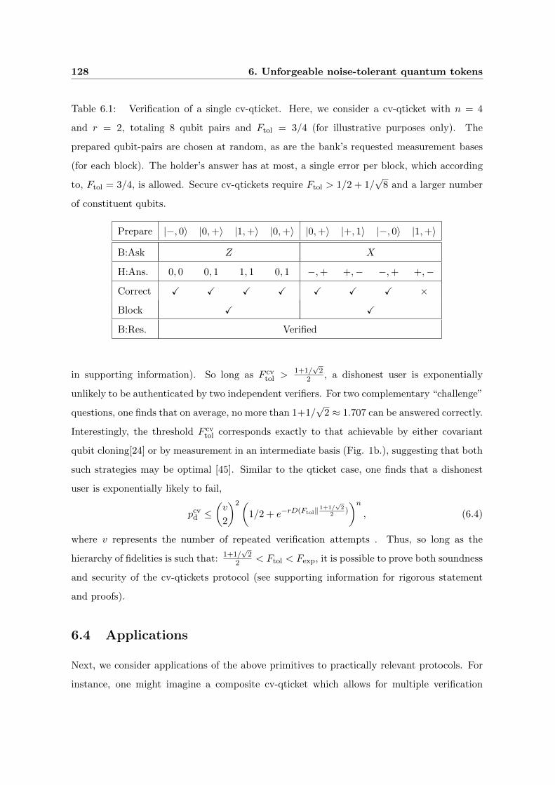
128 6. Unforgeable noise-tolerant quantum tokens
Table 6.1: Verification of a single cv-qticket. Here, we consider a cv-qticket with n = 4
and r = 2, totaling 8 qubit pairs and Ftol = 3/4 (for illustrative purposes only). The
prepared qubit-pairs are chosen at random, as are the bank’s requested measurement bases
(for each block). The holder’s answer has at most, a single error per block, which according
to, Ftol = 3/4, is allowed. Secure cv-qtickets require Ftol > 1/2 + 1/√
8 and a larger number
of constituent qubits.
Prepare |−, 0〉 |0,+〉 |1,+〉 |0,+〉 |0,+〉 |+, 1〉 |−, 0〉 |1,+〉
B:Ask Z X
H:Ans. 0, 0 0, 1 1, 1 0, 1 −,+ +,− −,+ +,−Correct X X X X X X X ×Block X X
B:Res. Verified
in supporting information). So long as F cvtol >
1+1/√
22 , a dishonest user is exponentially
unlikely to be authenticated by two independent verifiers. For two complementary “challenge”
questions, one finds that on average, no more than 1+1/√
2 ≈ 1.707 can be answered correctly.
Interestingly, the threshold F cvtol corresponds exactly to that achievable by either covariant
qubit cloning[24] or by measurement in an intermediate basis (Fig. 1b.), suggesting that both
such strategies may be optimal [45]. Similar to the qticket case, one finds that a dishonest
user is exponentially likely to fail,
pcvd ≤
(v
2
)2(1/2 + e−rD(Ftol‖ 1+1/
√2
2)
)n, (6.4)
where v represents the number of repeated verification attempts . Thus, so long as the
hierarchy of fidelities is such that: 1+1/√
22 < Ftol < Fexp, it is possible to prove both soundness
and security of the cv-qtickets protocol (see supporting information for rigorous statement
and proofs).
6.4 Applications
Next, we consider applications of the above primitives to practically relevant protocols. For
instance, one might imagine a composite cv-qticket which allows for multiple verification
6.5 Discussion 129
rounds while also ensuring that the token cannot be split into two independently valid subparts
[44]. Such a construction may be used to create a quantum-protected credit card. Indeed,
the classical communication which takes place with the issuer (bank) to verify the cv-qticket
(via “challenge” questions) may be intentionally publicized to a merchant who needs to be
convinced of the card’s validity. By contrast to modern credit card implementations, such
a quantum credit card would be unforgeable and hence immune to fraudulent charges (Fig.
2a).
An alternate advantage offered by the qticket framework is evinced in the case where veri-
fiers may not possess a secure communication channel with each other. Consider for example,
a dishonest user who seeks to copy multiple concert tickets, enabling his henchmen to enter
at different checkpoint gates. A classical solution would involve gate verifiers communicating
amongst one another to ensure that each ticket serial number is only allowed entry a single
time; however, as shown in Fig. 2b., such a safeguard can be overcome in the event that
communication has been severed. By contrast, a concert ticket based upon the proposed
qticket primitive would be automatically secure against such a scenario; indeed, the security
of qtickets is guaranteed even when verifiers are assumed to be isolated. Such isolation may
be especially useful for applications involving quantum identification tokens, where multiple
verifiers may exist who are either unable or unwilling to communicate with one another.
6.5 Discussion
While quantum primitives have been the subject of tremendous theoretical interest, their
practical realization demands robustness in the face of realistic imperfections. Our above
analysis demonstrates that such noise tolerance can be achieved for certain classes of unforge-
able quantum tokens. Moreover, the derived tolerance thresholds are remarkably mild and
suggest that proof of principle experiments are currently accessible in systems ranging from
trapped ions [60, 81] and superconducting devices [127, 46] to solid-state spins [36, 93, 14, 90].
In particular, recent advances on single nuclear spins situated in a compact room-temperature
solid, have demonstrated that ultra-long storage times can be attained in combination with
high fidelity initialization and readout [90]; such advances suggest that quantum devices based
upon single qubit quantum memories may be both practical and realistically feasible.
While our analysis has focused on describing a primitive based upon single tokens, natural
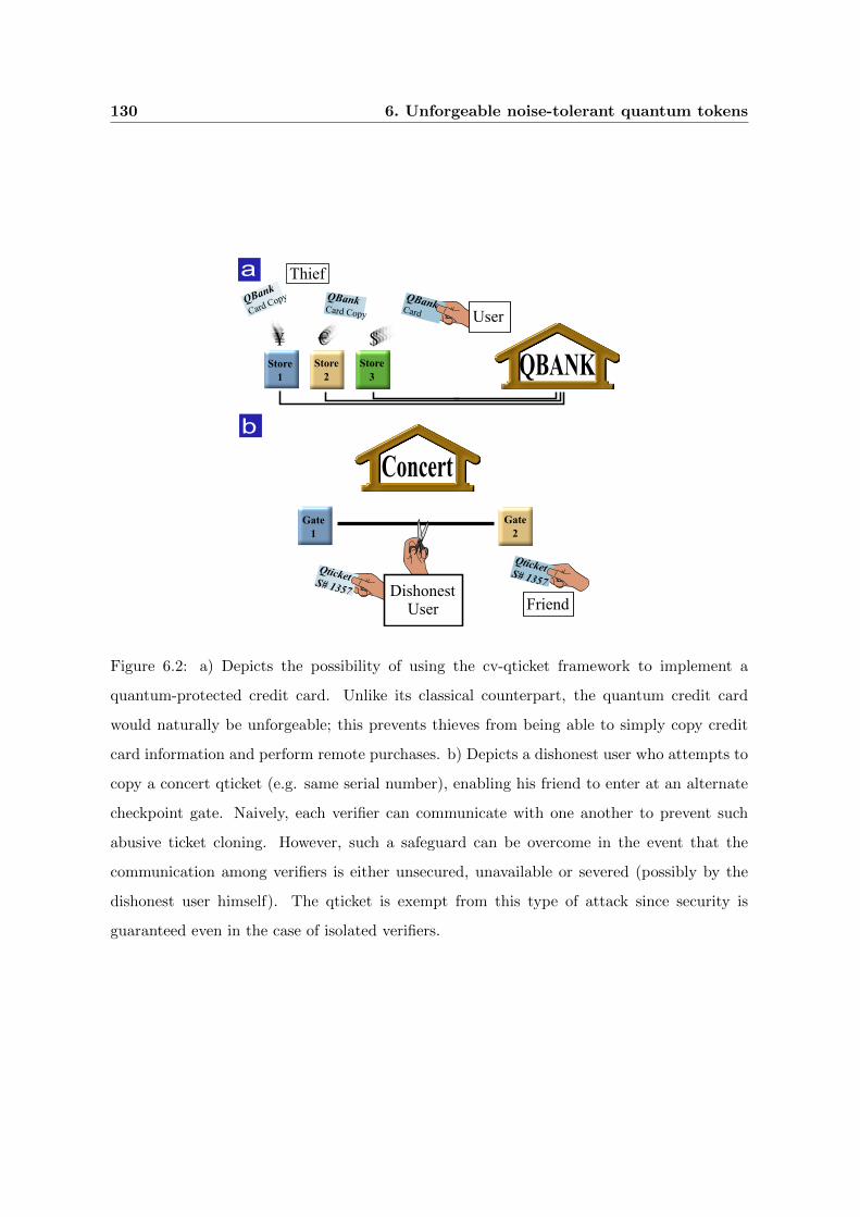
130 6. Unforgeable noise-tolerant quantum tokens
QBankCard
QBANK$€¥
Store 1
User
Store 2
Store 3
QticketS# 1357
Concert
Dishonest
Gate 1
User
Gate 2
QBank
Card Copy QBankCard Copy
Thief
QticketS# 1357
a
b
Friend
Figure 6.2: a) Depicts the possibility of using the cv-qticket framework to implement a
quantum-protected credit card. Unlike its classical counterpart, the quantum credit card
would naturally be unforgeable; this prevents thieves from being able to simply copy credit
card information and perform remote purchases. b) Depicts a dishonest user who attempts to
copy a concert qticket (e.g. same serial number), enabling his friend to enter at an alternate
checkpoint gate. Naively, each verifier can communicate with one another to prevent such
abusive ticket cloning. However, such a safeguard can be overcome in the event that the
communication among verifiers is either unsecured, unavailable or severed (possibly by the
dishonest user himself). The qticket is exempt from this type of attack since security is
guaranteed even in the case of isolated verifiers.
6.A Notation and external results 131
extensions to the case of multiple identical quantum tokens open up the possibility of even
more novel applications. In particular, as detailed in the supplementary information, it is
possible to extend our threshold results to the case where c identical copies of the quantum
token are issued. In this case, to ensure that the production of c + 1 valid tokens is ex-
ponentially improbable, the required threshold fidelity must be greater than 1 − 1(c+1)(c+2) .
The existence of such multiple identical tokens can provide a certain degree of anonymity
for users and could be employed in primitives such as quantum voting. A crucial question
that remains is whether a rigorous proof of anonymity can be obtained in a noisy environ-
ment. Furthermore, our proposed quantum tokens can also be seen as a basic noise tolerant
building block for implementing more advanced application schemes; such schemes can range
from novel implementations of quantum key distribution [16, 45, 49, 110] based upon physical
qubit transport to complex one-time-entry identification cards. Beyond these specific appli-
cations, a number of scientific avenues can be explored, including for example, understanding
whether an interplay between computational assumptions and quantum memories can yield
fundamentally new approaches to encryption.
6.A Notation and external results
The following definitions and external results will be used extensively throughout the proofs
and are included here to provide a self-contained presentation.
Definition A quantum state t-design is a probability distribution over pure quantum states
(pi, | ψi〉) such that ∑i
pi (| ψi〉〈ψi |)⊗t =
∫Haar
(| ψ〉〈ψ |)⊗t dψ.
In other words, a quantum state t-design duplicates the properties of the unique unitarily
invariant Haar measure over quantum states for all polynomials up to degree t. We will use
the set of states
Q = {| 0〉, | 1〉, | +〉, | −〉, | +i〉, | −i〉} (6.5)
with equal weights pi = 1/6; this constitutes a quantum state 3-design over H2 [132].
The average fidelity for a channel quantifies how well the channel preserves quantum
states.
132 6. Unforgeable noise-tolerant quantum tokens
Definition The Average fidelity of a map M is defined as
F (M) =
∫Haar〈ψ |M (| ψ〉〈ψ |) | ψ〉dψ.
Note for example that the average fidelity of a map M is expressed as a Haar integral of
a degree 2 polynomial expression in bras and kets and can thus be equated to a weighted
average over a quantum state 2-design.
Throughout the text, boolean values B = {True, False} will be represented as True :=
1, False := 0 and the negation b := 1 − b. We will also use the variable ~b to denote
boolean strings (i.e. ordered sequences of values in {0, 1}) with len(~b) denoting the length or
number of components of a sequence and tl(~b) denoting the string obtained from removing
the last element from ~b. We will denote by Pr[e] the probaility of an event e and Exp[v] the
expectation value of an expression v. Note that according to our convention, if the expression
is a boolean formula they may be used interchangeably.
The relative entropy is a distinguishability measure between two probability distributions.
It will be used extensively (particularly among binary or Bernoulli distributions) and appears
in the definition of auxiliary results. Let 0 ≤ p, q ≤ 1, by abuse of notation, we take D(p‖q) =
p ln pq + (1 − p) ln 1−p
1−q , the relative entropy between two Bernoulli probability distributions
with respective parameters p and q. Note that this definition satisfies D(p‖q) ≥ 2(p− q)2.
The following generalization of the Chernoff-Hoeffding bound derived by Panconesi and
Srinivasan [102] provides the same thesis as a standard Chernoff bound while relaxing the
hypothesis to allow dependent random variables.
Theorem 6.A.1 (Generalized Chernoff-Hoeffding bound) Let X1, . . . , Xn be Boolean {0, 1}random variables, such that for some δi and every S ⊆ {1, . . . , n}, it holds that Pr
[∧i∈S Xi
]≤∏
i∈S δi. Then for any γ ∈ [δ, 1] we have that Pr [∑n
i=1Xi ≥ γn] ≤ e−nD(γ‖δ), with δ :=
n−1∑n
i=1 δi.
A further generalization to real valued random variables will also be required. This is
adapted to our purpose from theorem 3.3 of Impagliazzo and Kabanets [61].
Theorem 6.A.2 Let X1, . . . , Xn be real valued random variables, with each Xi ∈ [0, 1]. Sup-
pose that there is a 0 ≤ δ ≤ 1 s.t., for every set S ⊆ {1, . . . , n}, Exp[∏
i∈S Xi
]≤ δ|S| and γ
s.t. δ ≤ γ ≤ 1 and γn ∈ N. Then we have that Pr [∑n
i=1Xi ≥ γn] ≤ 2e−nD(γ‖δ).
6.B Qtickets 133
6.B Qtickets
We first provide a rigorous definition of qtickets and how they are verified. We then proceed
to our claims, and the soundness, security and tightness of our security bound (accompanied
with respective proofs). Namely, we show that qtickets may be successfully redeemed by an
honest holder achieving a sufficiently good storage fidelity. We then show that a dishonest
holder will have a negligible chance of producing two qtickets which are accepted by verifiers
from a single valid qticket, even after repeated verification attempts. Finally we show how
a simple counterfeiting strategy has a high probability of producing two such qtickets if the
verification tolerance is set below the threshold value. As an extension, we consider how our
results generalize to producing multiple identical qtickets.
6.B.1 Definition of qtickets
Each qticket consists of a serial number s and an N component pure product state ρ(s) =⊗Ni=1 ρ
(s)i . For each serial number s, qticket components ρ
(s)i are chosen uniformly at random
from Q. This means qtickets ρ(s) are taken uniformly at random from the set Q = Q⊗N
(where by abuse of notation, the elements of Q are N component pure product states in
HQ = H⊗N2 , with components taken from Q). The verifiers store a database containing, for
each s, a classical description of ρ(s) kept secret from ticket holders and the general public.
In order to simplify notation, the serial number s associated to individual qtickets will be
omitted from now on.
In order to use qtickets, they are transferred to a verification authority who can either
accept or reject them. In both cases however, the qticket is not returned, only the binary
outcome of verification. The qticket protocol is additionally parametrized by the fraction
Ftol of qubits that a verification authority requires to be correct in order for verification to
succeed. In order to verify a submitted qticket ρ, a full measurement will be performed in
the product basis associated to the original qticket ρ and the number of correct outcomes is
then counted. If more than at least FtolN are correct, the (possibly noisy) submitted qticket
ρ is accepted, otherwise, it is rejected.
For any pure product state ρ =⊗N
i=1 ρi we define a projector P ρacc ∈ L(HQ) associated
to the subspace of states that would be accepted if ρ were a qticket (i.e. states coinciding
with ρ in at least a fraction Ftol of the qubits). The projector P ρacc offers a more abstract
134 6. Unforgeable noise-tolerant quantum tokens
interpretation and may be rigorously defined as
Acceptance projector Given a pure N qubit product state ρ =⊗N
i=1 ρi and a security
parameter 0 ≤ Ftol ≤ 1, we define the acceptance projector
P ρacc =∑
~b:∑bi≥FtolN
N⊗i=1
(biρi + biρ
⊥i
),
where ~b ∈ {0, 1}N is a boolean string.
By abused of notation, ρi and its orthogonal complement ρ⊥i := 12 − ρi are used as rank 1
projectors in L(H2).
6.B.2 Soundness
The soundness result states that even under imperfect storage and readout fidelity, legitimate
qtickets work well as long as the fidelity loss is not too severe. The completely positive trace
preserving (CPTP) maps Mi will be assumed to represent the encoding, storage and readout
of the i-th qubit component of the qticket. In this sense, the soundness statement takes place
at the level of single qubits. This is necessarily the case, since legitimate qtickets are ruined
if a significant fraction of the qubits fail in a correlated way. Given Fi = F (Mi), the average
fidelity of the qubit map Mi, we define Fexp := N−1∑Fi to be the average qubit fidelity
of the full map M =⊗
iMi over all components. The probability that the “noisy” qticket
resulting from this map is accepted as valid is given by ph(M) = 1|Q|∑
ρ∈Q tr [P ρaccM (ρ)].
Theorem 6.B.1 (Soundness of qtickets) As long as Fexp > Ftol, an honest holder can suc-
cessfully redeem qtickets with a probability
ph(M) ≥ 1− e−ND(Ftol‖Fexp).
Proof. Consider the boolean random variables ~X = (X1, . . . , XN ) with joint distribution
given by
Pr[ ~X = ~b] =1
|Q|∑ρ∈Q
tr
[M(ρ)
N⊗i=1
(biρi + biρ
⊥i
)]. (6.6)
Since M =⊗
iMi, we may recast equation 2 as
Pr[ ~X = ~b] =
N∏i=1
1
6
∑ρi∈Q
tr[Mi(ρi)(biρi + biρ
⊥i )]
(6.7)

6.B Qtickets 135
Since Q is a quantum state 2-design over qubit space, each factor coincides with the definition
of the average fidelity Fi of Mi if bi = 1 and with 1−Fi if bi = 0. Hence the Xi are independent
boolean random variables with probability Pr[Xi] = Fi. Moreover, according to definition
6.B.1, we have 1|Q|∑
ρ∈Q tr[P ρaccM(ρ)] = Pr[∑N
i=1Xi ≥ FtolN ]. Since the Xi are independent,
a standard Chernoff-Hoeffding bound allows us to conclude.
6.B.3 Security
Consider the probability of producing two tokens, both passing verification by means of the
most general possible transformation, a CPTP map T , applied on a single genuine qticket.
Definition (Counterfeiting fidelity) We define the average counterfeiting fidelity of a map
T ∈ HQ → H⊗2Q as
pd(T ) =1
|Q|∑ρ∈Q
tr[(P ρacc)
⊗2 T (ρ)]
(6.8)
One of our main results states that as long as the verification threshold Ftol is set suffi-
ciently high (> 5/6), a counterfeiter will have negligible (exponentially small in N) chances
of producing two verified tokens from a single genuine original.
Theorem 6.B.2 (Security of qtickets) For Ftol > 5/6 and for any CPTP map T ∈ HQ →H⊗2Q we have that
pd(T ) ≤ e−ND(2Ftol−1‖2/3). (6.9)
Most of the work for proving this goes into excluding the possibility that a non-product
counterfeiting strategy could perform significantly better than any product strategy such as
performing optimal cloning on each individual qubit. That is, we take into account the fact
that the map T need not factorize with respect to the different components of the qticket.
Note also that D(2Ftol − 1‖2/3) = 0 precisely for Ftol = 5/6 and is positive otherwise. Fi-
nally, we prove that even if the holder of a qticket attempts to perform v succesive verification
attempts (each time possibly using information learned from the acceptance/rejection of pre-
vious attempts) the chances of having two or more submitted qtickets accepted grows by no
more than a factor of(v2
).

136 6. Unforgeable noise-tolerant quantum tokens
Theorem 6.B.3 (Security of qtickets with learning) If the holder of a valid qticket submits
v tokens for verification, the probability of having two or more accepted is upper bounded by
pd,v =
(v
2
)e−ND(2Ftol−1‖2/3).
Note that since(v2
)is a polynomial of degree 2 in v, this bound still allows for an exponentially
large number (in N) of qticket submissions v, while preserving exponentially good security.
Proof outline
We now outline the proof for theorems 6.B.2 and 6.B.3. First, the claim in theorem 6.B.2 is
equated to an equivalent one, which averages over the set of all pure product states instead
of Q. We then bound the average cloning probability by (2/3)N for the set of pure product
states following the lines of R. F. Werner [128] for the optimal cloning of pure states. From
there, the generalized Chernoff bound from theorem 6.A.1 for dependent random variables
allows us to derive the desired result. The result of theorem 6.B.3 is obtained from a counting
argument relating the security of multiple verification attempts with the static counterfeiting
fidelity bound of theorem 6.B.2.
Equivalence with continuous statement
For the qticket protocol, drawing each component from a discrete set of states is required in
order to provide an efficient classical description. However, certain statements are simpler to
analyze over the full set of pure product states. This is the case for the counterfeiting fidelity,
which can also be expressed as a uniform average over all pure product states.
Lemma 6.B.4 (Counterfeiting fidelity) The average counterfeiting fidelity of a map T can
be expressed as
pd(T ) =
∫d~ρ tr
[(P ~ρacc
)⊗2T (~ρ)
](6.10)
where∫d~ρ represents N nested integrations on the Haar measure of qubit components and ~ρ
the resulting product state.
Proof. Definition 6.B.1 may seem unnecessarily cumbersome, yet it serves to make explicit
that the projector P ρacc is a polynomial of degree 1 in each of the components ρi of the qticket
ρ. Furthermore, note that regardless of what the multi-qubit map T is, its application T (ρ)
6.B Qtickets 137
has degree 1 in each of the components ρi of ρ. Together this implies that the integrand
of lemma 6.B.4 is a polynomial of degree at most 3 in each of the qubit components ρi of
~ρ. We may conclude by observing that the average taken in definition 6.B.3 is equivalent to
uniformly taking each component ρi from a qubit state 3-design.
Optimal cloning for pure product states
R. F. Werner [128] obtained a tight upper bound for the average probability of a CPTP map
T producing m clones from n copies of an unknown pure quantum state | ψ〉. Our statement
is that if one attempts to clone an N component pure product state, the optimal cloning
probability is achieved by independently cloning each of the components; neither generating
entanglement nor correlations may help with the cloning. We present this statement for the
case of cloning two copies from a qubit product state, but the derivation is fully generalizable.
Lemma 6.B.5 (Optimal cloning of pure product states) The average cloning fidelity over N
qubit component pure product states of a CPTP map T is bounded by∫d~ρtr[~ρ⊗2T (~ρ)] ≤ (2/3)N .
Proof. One possible derivation of this lemma is by following the lines of the original proof
for optimal cloning of pure states [128]. First one shows that if there is a CPTP map T
achieving average cloning fidelity F ? then there is a covariant CPTP map T ? achieving the
same average cloning fidelity. This map can be explicitly constructed as
T ?(~ρ) =
∫d~g ~g†⊗2T (~g~ρ~g†)~g⊗2, (6.11)
where the integral∫d~g averages over all possible local rotations ~g on N subsystems. This
covariant map achieves exactly the same cloning fidelity for any initial pure product state
since all pure product states are equivalent up to local unitaries. Finally, we observe
0 ≤ tr[~ρ⊗2T ?(12N − ~ρ)] (6.12)
since 12N − ~ρ is positive and T ? positivity preserving. We then obtain
F ? ≤ tr[~ρ⊗2T ?(12N )] (6.13)
138 6. Unforgeable noise-tolerant quantum tokens
and may now average this inequality over ~ρ and use∫d~ρ ~ρ⊗2 =
(S2)⊗N
3N, (6.14)
where S2 is the rank 3 projector onto the symmetric space of two qubits. The operator norm
of this expression is 1/3N whereas tr[T ?(12N )] ≤ 2N leading to F ? ≤ (23)N , as desired.
Pigeonhole argument and Chernoff bound
We are now ready to prove the first no-counterfeiting result for qtickets.
Proof of theorem 6.B.2. Consider the boolean random variables ~E = (E1, . . . , EN ) with
joint distribution given by
Pr[ ~E = ~b] =
∫d~ρtr
[T (~ρ)
N⊗i=1
(biρ⊗2i + bi(14 − ρ⊗2
i ))]. (6.15)
Intuitively, the variable Ei represents the event of measuring the i-th component to be cor-
rectly cloned.
In order for the two qtickets to be accepted, there must be a total of at least FtolN com-
ponents yielding the correct measured outcome in each qticket. By the pigeonhole principle,
this means that there are at least 2FtolN −N components which were measured correctly on
both submitted qtickets,
pd(T ) ≤ Pr
[N∑i=1
Ei ≥ (2Ftol − 1)N
]. (6.16)
For arbitrarily chosen T , the Ei may be dependent variables. However, according to lemma
6.B.5, for any subset S of qubit components, we may bound
Pr[∀i∈SEi] ≤(
2
3
)|S|. (6.17)
Theorem 6.A.1, is now invoked to provide an upper bound on the RHS of eq. 6.16, yielding
the thesis of theorem 6.B.2.
Combinatorial bound on learning
The bound on counterfeiting that we have provided assumes that two (possibly entangled)
counterfeits are produced by applying a CPTP map on a single original copy. In contrast, a
sequential strategy temporally orders the submitted qtickets where the production strategy

6.B Qtickets 139
(CPTP map) for the later submissions can depend on whether previous submissions where
accepted or not. The counterfeiter may learn valuable information about how to construct
valid qtickets from the feedback provided by the verifiers. The content of theorem 6.B.3 is
that even with a valid qticket and the information learned from v repeated submissions it is
very unlikely for a counterfeiter to produce more than one accepted qticket.
Proof of theorem 6.B.3. According to theorem 6.B.2, the probability pd(T ) for any
CP map T to produce two valid counterfeit copies from a single one, is upper bounded by
B = e−ND(2Ftol−1‖2/3). We bound the counterfeiting probability of an interactive strategy
S submitting v tokens for verification by the sum of the counterfeiting fidelity of(v2
)CP
maps Tk,l. Each of these maps corresponds to the case in which a specific pair {k, l} of the v
submitted tokens are the first to be accepted by the verifiers.
Without loss of generality, we assume that in an interactive strategy the holder waits
for the outcome of the j-th verification in order to decide how to continue and produce the
j + 1-th submission. We model a v step interactive strategy S as a collection of CPTP maps
{S~b} with ~b a boolean string of length between 0 and v−1 representing what the counterfeiter
does after receiving the first len(~b) verification outcomes.
Each S~b is a CPTP map fromHH toHQ⊗HH , whereHQ is a Hilbert space accommodating
qtickets and HH is a larger space representing the memory of the holder.
For any partial verification result~b we may write the CPTP map which produces the len(~b)
submissions as Stl(~b)
, which is composed of successively applying S~b′ for all initial substrings
~b′ of ~b. That is
S∅ :=S∅
S~b :=(
id⊗ len(~b)Q ⊗S~b
)◦ S
tl(~b).
(6.18)
For an interactive strategy S the probability that the first len(~b) verification outcomes are
given by ~b is expressed as
p~b(S) =1
|Q|∑ρ∈Q
tr[Stl(~b)
(ρ)
len(~b)⊗j=1
(bjP
ρacc + bjP
ρrej
)⊗ 1H ], (6.19)
where P ρrej := 1Q − P ρacc. The probability for the interactive strategy S to succeed at coun-
terfeiting in v steps can be described as the sum of these probabilities over all possible full
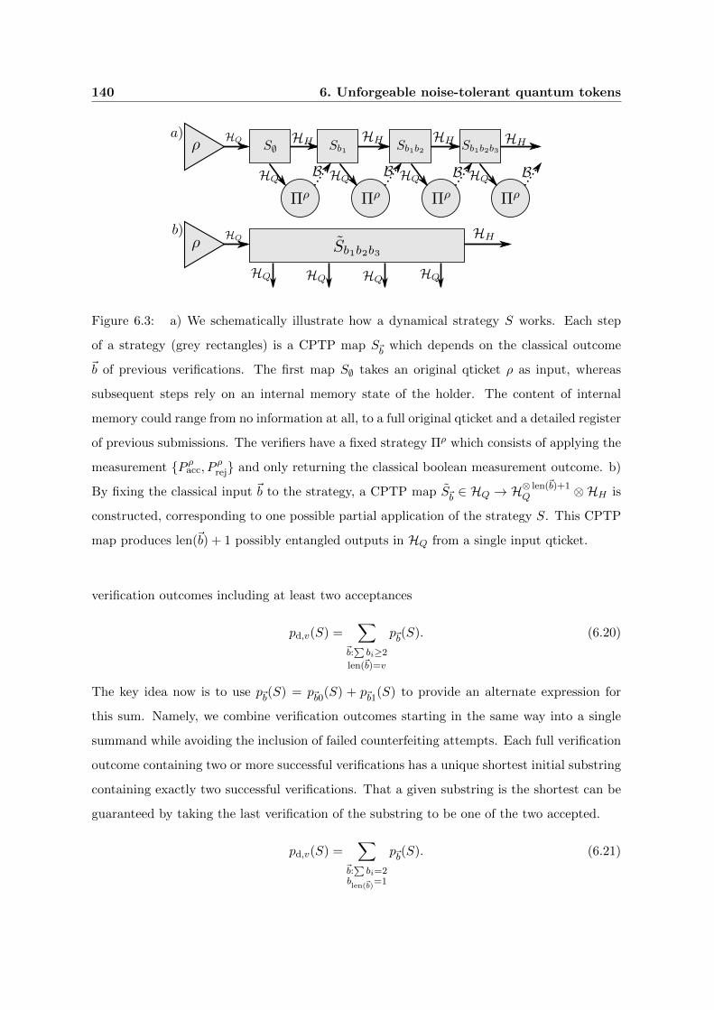
140 6. Unforgeable noise-tolerant quantum tokens
Figure 6.3: a) We schematically illustrate how a dynamical strategy S works. Each step
of a strategy (grey rectangles) is a CPTP map S~b which depends on the classical outcome
~b of previous verifications. The first map S∅ takes an original qticket ρ as input, whereas
subsequent steps rely on an internal memory state of the holder. The content of internal
memory could range from no information at all, to a full original qticket and a detailed register
of previous submissions. The verifiers have a fixed strategy Πρ which consists of applying the
measurement {P ρacc, Pρrej} and only returning the classical boolean measurement outcome. b)
By fixing the classical input ~b to the strategy, a CPTP map S~b ∈ HQ → H⊗ len(~b)+1Q ⊗HH is
constructed, corresponding to one possible partial application of the strategy S. This CPTP
map produces len(~b) + 1 possibly entangled outputs in HQ from a single input qticket.
verification outcomes including at least two acceptances
pd,v(S) =∑
~b:∑bi≥2
len(~b)=v
p~b(S). (6.20)
The key idea now is to use p~b(S) = p~b0(S) + p~b1(S) to provide an alternate expression for
this sum. Namely, we combine verification outcomes starting in the same way into a single
summand while avoiding the inclusion of failed counterfeiting attempts. Each full verification
outcome containing two or more successful verifications has a unique shortest initial substring
containing exactly two successful verifications. That a given substring is the shortest can be
guaranteed by taking the last verification of the substring to be one of the two accepted.
pd,v(S) =∑
~b:∑bi=2
blen(~b)
=1
p~b(S). (6.21)

6.B Qtickets 141
Each of the(v2
)summands on the RHS of Eq. (S6.21), may be characterized by two indices
k, l s.t.
~b =
k−1︷ ︸︸ ︷0 . . . 0 1
l−k−1︷ ︸︸ ︷0 . . . 0 1 for some k < l ≤ v. (6.22)
For each one of these summands, we construct a static strategy Tk,l(ρ) = tr\k,l[Stl(~b)(ρ)] which
takes as input a single valid qticket ρ and submits exactly two tokens. The counterfeiting
probability of this map on ρ is
tr[(P ρacc)
⊗2 Tk,l(ρ)]
=tr[(P ρacc)
⊗2 tr\k,l[Stl(~b)(ρ)]]
=tr[Stl(~b)
(ρ)
len(~b)⊗j=1
(bjP
ρacc + bj1Q
)⊗ 1H ]
≥tr[Stl(~b)
(ρ)
len(~b)⊗j=1
(bjP
ρacc + bjP
ρrej
)⊗ 1H ].
(6.23)
By averaging over ρ ∈ Q we obtain p~b(S) ≤ pd(Tk,l) ≤ B and invoking Eq. (S6.21) we obtain
pd,v(S) ≤(v2
)B.
6.B.4 Tightness
For Ftol < 5/6 applying an optimal qubit cloning map[128] Λ(ρ) = 13ρ⊗ ρ+ 1
6ρ⊗ 1+ 161⊗ ρ
on each of the individual qubits of the qticket provides a good counterfeiting probability.
The plot in Fig. S6.4 illustrates the probability of counterfeiter to actually get two qtickets
accepted when taking this approach. For each of the two counterfeited qtickets, the probability
of failing verification is the cumulant of a binomial distribution B(N, 5/6) up to FtolN and
rejection probability may be upper bounded by 12 exp(−2N(5/6 − Ftol)
2) using Hoeffding’s
inequality. Even when failure of the two qtickets is anticorrelated, the probability of either of
them failing verification can not excede the sum. This shows that a the scheme can not be
made secure for Ftol < 5/6. While such a scheme provides optimal forging probability when
(Ftol = 1), other schemes could in principle outperform it in terms of counterfeiting capability.
Althought this is in principle possible, our security result shows that assymptotically in N ,
no other strategy may work for Ftol > 5/6.
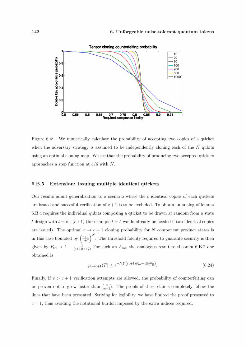
142 6. Unforgeable noise-tolerant quantum tokens
0.5 0.55 0.6 0.65 0.7 0.75 0.8 0.85 0.9 0.95 10
0.2
0.4
0.6
0.8
1
Required acceptance fidelity
Dou
ble
key
acce
ptan
ce p
roba
bilit
y
Tensor cloning counterfeiting probability
0.5 0.55 0.6 0.65 0.7 0.75 0.8 0.85 0.9 0.95 10
0.2
0.4
0.6
0.8
1
Required acceptance fidelity
Dou
ble
key
acce
ptan
ce p
roba
bilit
y
Tensor cloning counterfeiting probability
0.5 0.55 0.6 0.65 0.7 0.75 0.8 0.85 0.9 0.95 10
0.2
0.4
0.6
0.8
1
Required acceptance fidelity
Dou
ble
key
acce
ptan
ce p
roba
bilit
y
Tensor cloning counterfeiting probability
0.5 0.55 0.6 0.65 0.7 0.75 0.8 0.85 0.9 0.95 10
0.2
0.4
0.6
0.8
1
X: 0.848Y: 0.14
Required acceptance fidelity
Dou
ble
key
acce
ptan
ce p
roba
bilit
y
Tensor cloning counterfeiting probability1020501002005001000
0.5 0.55 0.6 0.65 0.7 0.75 0.8 0.85 0.9 0.95 10
0.2
0.4
0.6
0.8
1
Required acceptance fidelity
Dou
ble
key
acce
ptan
ce p
roba
bilit
y
Tensor cloning counterfeiting probability
1020501002005001000
Figure 6.4: We numerically calculate the probability of accepting two copies of a qticket
when the adversary strategy is assumed to be independently cloning each of the N qubits
using an optimal cloning map. We see that the probability of producing two accepted qtickets
approaches a step function at 5/6 with N .
6.B.5 Extension: Issuing multiple identical qtickets
Our results admit generalization to a scenario where the c identical copies of each qtickets
are issued and succesful verification of c+ 1 is to be excluded. To obtain an analog of lemma
6.B.4 requires the individual qubits composing a qticket to be drawn at random from a state
t-design with t = c+(c+1) (for example t = 5 would already be needed if two identical copies
are issued). The optimal c → c + 1 cloning probability for N component product states is
in this case bounded by(c+1c+2
)N. The threshold fidelity required to guarante security is then
given by Ftol > 1 − 1(c+1)(c+2) For such an Ftol, the analogous result to theorem 6.B.2 one
obtained is
pc→c+1(T ) ≤ e−ND((c+1)Ftol−c‖ c+1c+2). (6.24)
Finally, if v > c + 1 verification attempts are allowed, the probability of counterfeiting can
be proven not to grow faster than(vc+1
). The proofs of these claims completely follow the
lines that have been presented. Striving for legibility, we have limited the proof presented to
c = 1, thus avoiding the notational burdon imposed by the extra indices required.
6.C CV-Qtickets 143
6.C CV-Qtickets
In this section we provide a proof that cv-qtickets are secure, not only against counterfeiting
but also against any other possible double usage. We first present definitions for cv-qtickets
and their verification. We then state the associated soundness and security guarantees and
outline the security proof. Only the proof of the security statement is provided, since prov-
ing soundness for cv-qtickets requires no additional techniques as compared to soundness of
qtickets.
6.C.1 CV-Qticket definition
Each cv-qticket is composed of n× r qubit pairs. Each qubit pair is prepared by choosing a
state from
{|0,+〉, |0,−〉, |1,+〉, |1,−〉, |+, 0〉, |−, 0〉, |+, 1〉, |−, 1〉}
uniformly at random.
A full verification question for the cv-qticket will consist of n randomly chosen axes from
{X,Z} each corresponding to a specific block of r qubit pairs. In principle, the holder of the
cv-qticket then measures the polarization of every qubit components along the corresponding
requested axis and communicates the measurement outcomes to the verifier. The criteria
to consider an answer correct is the following; within each of the n blocks, at least Ftolr of
the reported outcomes corresponding to qubits prepared in a polarization eigenstate of the
inquired axis should be given correctly.
6.C.2 Soundness
The soundness result states that even under imperfect storage and readout fidelity, legitimate
cv-qtickets work well as long as the fidelity loss is not too severe. Again, the completely pos-
itive trace preserving (CPTP) maps Mj will be assumed to represent the encoding, storage
and readout of the j-th qubit component of the cv-qticket, with the full map over all compo-
nents given by M =⊗
j∈{1,...,2r×n}Mj . In the case of cv-qtickets, sufficiently many (Ftolr)
correct answers should be provided within each block, demanding that a sufficiently good
average fidelity be implemented for every single block. A random remapping of the Cartesian
axes for each qubit component of a cv-qticket is also necessary, and can be achieved via a
144 6. Unforgeable noise-tolerant quantum tokens
random unitary (possibly from a unitary 2-design). This is required for example in the case
where an actual physical polarization, say X, is lost faster than other components. In this
case asking for the stored X polarization for all qubits in a block may yield a large failure
probability even though the average storage fidelity among the qubits is sufficiently high. A
random unitary remapping solves this and allows to connect with the average qubit storage
fidelity, even in the case where only two nominal axes are used.
Given Fj = F (Mj), the average fidelity of the qubit map Mj , we define Fexp,b :=
N−1∑
j:d j2re=b Fj to be the average qubit fidelity within block b ∈ {1, . . . , n}. Furthermore,
to simplify the final expression, let us define Fexp = minb Fexp,b.
Theorem 6.C.1 (Soundness of cv-qtickets) As long as Fexp > Ftol, an honest holder imple-
menting a map M can successfully redeems cv-qtickets with a probability
pcvh (M) ≥
(1− e−rD(Fexp‖Ftol)
)n.
Observe that one may reduce this statement to n independent statements within each block
which are completely analogous to the soundness for qtickets theorem 6.B.1.
6.C.3 Security
A naive security statement expresses that the holder of a single cv-qticket is unable to produce
two copies from it, each with the potential of passing a verification. Since the verification of
cv-qtickets is achieved by sending a classical message to a verifier, the security statement for
cv-qtickets goes beyond this; it states that even with simultaneous access to two randomly
chosen verification questions, the holder of a cv-qticket is exponentially unlikely to provide
satisfactory answers to both. We further extend our security claim, to an even more adverse
scenario; the holder of a cv-qticket has simultaneous access to v independent verification ques-
tions and may proceed to answer them in any chosen order. Moreover failing in verification
attempts does not forbid the holder from further attempts which may possibly be performed
relying on the information accumulated from previous verification outcomes.
Let S be a mathematical object denoting the counterfeiting strategy taken by the holder
of a valid cv-qticket. We will denote by pcvd,v(S), the probability that strategy S leads to
two or more successful verifications when engaging in v verification attempts with possibly
independent verifiers. The probability is taken over the random generation of cv-qtickets, of
6.C CV-Qtickets 145
verification questions, and of measurement outcomes (Born’s rule). The security statement
is then
Theorem 6.C.2 (Security of cv-qtickets) For any counterfeiting strategy S and tolerance
parameter Ftol >1+1/
√2
2 we have
pcvd,v(S) ≤
(v
2
)2(1/2 + e−rD(Ftol‖ 1+1/
√2
2)
)n.
The proof of this statement goes as follows. Since abstractly cv-qtickets consist of a set of
randomly produced states and questions requested on these states the formalism of quantum
retrieval games (QRGs) provides adequate modeling. This framework is presented in a largely
self-contained manner, since its generality and potential make it of independent interest. We
first provide basic definitions for QRGs and derive some simple results. Then we present
possible ways of composing QRGs together with associated quantitative bounds. The first
results are then applied to the qubit pair constituents of cv-qtickets to bound the holders
potential to provide answers to complementary question. Cv-qtickets are then modeled by
a QRG for scenarios in which the holder of a cv-qticket wishes to simultaneously answer
questions from two independent verifiers without any additional aid. Finally, a combinatorial
bound, similar to the one used for qtickets, is used to provide an upper limit on how the
double verification probability may increase with the number v of verification attempts.
6.C.4 Quantum retrieval games
Quantum retrieval games (QRGs), recently defined by Gavinsky [44] provide a framework to
analyze protocols in which information is to be extracted from a state produced according
to a classical probability distribution. We will here present a definition of QRGs following
Gavinsky as well as some additional results derived which may be of independent interest.
Alice prepares a normalized state ρs = %(s)/ps according to the probability ps := tr[%s]
and transfers it to Bob. Whereas Alice remembers the index s of the generated state, Bob is
only provided with ρs and a full description of the distribution from which it was generated.
Alice then asks Bob a question about s which Bob attempts to answer as best as possible.
A simple possibility is for Alice to directly ask Bob the value of s. In general however,
the set of possible answers A need not coincide with the set of indexes S over the possible
prepared states. If each answer a is either correct or incorrect the question may be modeled

146 6. Unforgeable noise-tolerant quantum tokens
as σ ∈ S × A → {0, 1}. This is, σ(s, a) = 1 iff the answer a is correct for state index s
and σ(s, a) = 0 otherwise. This definition faithfully represents Gavinsky’s QRGs. We extend
this notion to weighted quantum retrieval games (WQRGs) to model situations where some
answers are “more correct” than others. Here for each prepared state s and possible answer
a the game will assign a non-negative real value σ(s, a) associated to the utility function of
answer a given input s (i.e. σ ∈ S ×A→ R+).
Bob needs to choose an answer a ∈ A and may use his copy of state ρs to do so. The most
general strategy that Bob can take according to the laws of quantum mechanics is to perform
a positive operator valued measurement (POVM). We will consider post-selected POVMs, as
opposed to a physical POVM, as those which may fail to produce a measurement outcome.
This is, whereas a physical POVM always produces an outcome from the expected set, for
post-selected POVM some “invalid” outcomes are discarded and excluded from statistics.
In order to express the random preparation of states by Alice we first define the notion of
an indexed ensemble.
Indexed ensemble We will say that % is an ensemble on H indexed over S iff ∀s ∈ S : %(s)
is a positive operator on H and∑
s∈S tr[%(s)] = 1.
Note that if % is an indexed ensemble, then ρ =∑
s %(s) is a normalized density matrix.
Although Alice gives a specific state %(s)/tr[%(s)] to Bob, since Bob does not know s, he does
not know which one has been received. The state ρ = trAlice[∑
s∈S s⊗ %(s)] will be called the
reduced density matrix of % since it corresponds to tracing out Alice’s classically correlated
subsystem containing the index s. Without loss of generality, ρ can be assumed to be full
rank on H.
In other words, a physical/selective projection P indexed over A is simply a physical/post-
selected POVM equipped with an interpretation for each possible measurement outcome in
terms of possible answers in a ∈ A.
Selective and physical projections We will say that P is a selective projection indexed
over A iff ∀a ∈ A, P(a) are bounded positive semidefinite operators on H. It will also be a
physical projection iff∑
a P(a) = 1.
Note that no normalization has been imposed for selective projections since induced proba-
bility distributions are normalized a posteriori. An indexed ensemble and a projection on the
6.C CV-Qtickets 147
same Hilbert space induce a joint probability distribution over the indexes S×A of prepared
states and provided answers.
Induced probability distribution Let % be an ensemble on H indexed over S and let Pbe a projection on H indexed over A. Then
p(s0, a0) =tr[P(a0)%(s0)]∑s,a tr[P(a)%(s)]
. (6.25)
is a probability distribution over S ×A which will be denoted by p = 〈%,P〉 and is undefined
unless∑
s,a Tr[P(a)%(s)] > 0.
Furthermore, note that for physical projections the denominator in Eq. (S6.25) is 1 and
the marginal of the resulting distribution over S is p(s) =∑
a p(s, a) = tr[%(s)] which is
independent of P.
Weighted quantum retrieval games Let % be an ensemble onH indexed over S. Consider
a utility function σ ∈ S×A→ R+. Then the pair G = (%, σ) is a weighted quantum retrieval
game. A WQRG is also a QRG when σ ∈ S ×A→ {0, 1}.
The value of a game G w.r.t. a projection P is the average utility obtained by Bob by
using a certain measurement strategy P. This value is given by the expectancy of the utility
function σ over the joint distribution of prepared states and measurement outcomes.
Definition The value of game G = (%, σ) w.r.t. projection P is defined as
Val(G,P) :=∑s,a
p(s, a)σ(s, a) (6.26)
where p = 〈%,P〉 is the induced probability distribution.
We now define the optimum value achievable by Bob for two distinct conditions depending
on whether selective or physical projections are allowed.
Definition The selective (respectively physical) value of a game G are defined as
Sel(G) := supP∈Selective projections
Val(G,P) (6.27)
Phys(G) := supP∈Physical projections
Val(G,P). (6.28)
148 6. Unforgeable noise-tolerant quantum tokens
Note that according to this definition Sel(G) ≥ Phys(G) since the supremum is taken over a
larger set. However, for certain tailored games, the selective and physical values will coincide.
The advantage of selective values is that they may be straightforwardly computed and are
more amenable to compositional results. If Bob is forced to provide an answer, he can only
achieve the physical value of a game. If Bob is allowed to abort the game after measuring his
state ρs and aborted games are not considered when calculating his expected utility then he
will be able to achieve the selective value.
The following result provides an explicit formula to calculate the selective value of a game.
In this sense, it is a generalization of lemma 4.3 in [44].
Theorem 6.C.3 (Selective value of a game) Let G = (%, σ) be a WQRG with∑
s %(s) =
ρ. Define O(a) :=∑
s σ(s, a)ρ−1/2%(s)ρ−1/2. Then the selective value of G may be calculated
as Sel(G) = maxa ‖O(a)‖, where ‖ · ‖ denotes the operator norm.
Proof. We first use the definition of the value of a game G w.r.t. P, expand the induced
probability distribution and move the sum over s inside the trace
Val(G,P) =
∑a Tr[P(a)
∑s σ(s, a)%(s)]∑
a tr[P(a)∑
s %(s)]. (6.29)
We define P such that P(a) = ρ1/2P(a)ρ1/2. Using this definition and that of ρ and Oa we
may rewrite
Val(G,P) =
∑a Tr[P(a)O(a)]∑
a Tr[P(a)]
≤ maxa
Tr[P(a)O(a)]
Tr[P(a)]
≤ maxa‖O(a)‖.
(6.30)
The first inequality uses the positivity of all summands. For the second inequality we note
that P(a) must be positive semidefinite and the variational definition of operator norm of
the positive semidefinite operator O(a). Equality can be achieved by taking P(a0) to be a
projector onto the highest eigenvalue subspace of O(a0) if ‖O(a0)‖ = maxa ‖O(a)‖ and taking
P(a0) = 0 otherwise.
The theorem provides an explicit construction of a projection achieving the selective value
of a game. Furthermore, the proof allows us to derive a necessary and sufficient condition
under which the selective and physical values of a game coincide.
6.C CV-Qtickets 149
Corollary 6.C.4 Given a retrieval game G, we have that Sel(G) = Phys(G) iff there exist
positive P(a) such that
O(a)P(a) = Sel(G)P(a) and∑a
P(a) = ρ (6.31)
We now turn to the systematic composition of retrieval games in the form of product and
threshold games. This provides a way to construct more elaborate retrieval games together
with bounds on their associated values. A natural definition of tensor product may be given
for indexed ensembles, projections and utility functions.
(%1 ⊗ %2)(s1, s2) = %1(s1)⊗ %2(s2) (6.32)
(P1 ⊗ P2)(a1, a2) = P1(a1)⊗ P2(a2) (6.33)
(σ1 ⊗ σ2)((s1, s2), (a1, a2)) = σ1(s1, a1)σ2(s2, a2) (6.34)
These definitions have the property that the tensor product of physical projections is a physical
projection and that the induced probability distribution of two tensor product is the tensor
product of the individual induced probability distributions
〈(%1 ⊗ %2), (P1 ⊗ P2)〉 = 〈%1,P1〉 ⊗ 〈%2,P2〉
Tensor product WQRG Let G1 = (%1, σ1) and G2 = (%2, σ2). We define the tensor product
WQRG G1 ⊗ G2 as
G1 ⊗ G2 = (%1 ⊗ %2, σ1 ⊗ σ2).
Proposition 6.C.5 (Tensor product selective value) The selective value of a tensor prod-
uct game is the product of the selective value of the independent games.
Sel(G1 ⊗ G2) = Sel(G1) Sel(G2)
Proof. By using the definition of O(a) in theorem 6.C.3 with respect to the WQRG involved
we obtain
‖O(a1, a2)‖ = ‖O1(a1)⊗O2(a2)‖ = ‖O1(a1)‖‖O2(a2)‖.
Maximizing over a1 and a2 on both sides theorem 6.C.3 provides the desired equality.
The selective value of the product game is attained by the tensor product of projections,
each achieving the respective selective values.
150 6. Unforgeable noise-tolerant quantum tokens
Corollary 6.C.6 (Tensor product physical value) If Phys(G1) = Sel(G1) and Phys(G2) =
Sel(G2) then Phys(G1 ⊗ G2) = Sel(G1 ⊗ G2).
Given a direct product game and a projection for it one may consider the inverse procedure
of defining a projection on one of the subcomponents of the game.
Restriction of a projection Let P be a projection on H1 ⊗ H2 indexed over A1 × A2.
Furthermore, let ρ2 be a normalized density matrix on H2. We define the restriction P|1 with
respect to ρ2 and A2 as
P|1(a1) =∑a2
tr2(P(a1, a2)1⊗ ρ2).
By abuse of notation, if ρ = ρ1 ⊗ ρ2 is a normalized product state in H1 ⊗H2 we may define
the restriction of P with respect to the normalized tensor factors of ρ. This is the case for the
reduced density matrix of product indexed ensembles. By restricting a projection one obtains
a new projection which induces the same reduced probability distribution
Lemma 6.C.7 (Restriction of a projection) Let P|1 be the restriction of P with respect
to ρ2 and A2, where ρ2 is the reduced density matrix of %2. Then
〈%1,P|1〉(s1, a1) =∑s2,a2
〈%1 ⊗ %2,P〉(s1s2, a1a2).
Theorem 6.C.8 (Selective value of threshold QRG) Let Gj = (%j , σj) be WQRGs s.t.
σj ∈ (Sj , Aj) → [0, 1] and Sel(Gj) = δj for all j ∈ {1, . . . , n}. Furthermore take δ =
n−1∑n
j=1 δj and δ ≤ γ ≤ 1. Define the QRG Gγ = (⊗
j %j), σγ) with a tensor product
ensemble distribution and boolean utility function
σγ(~s,~a) =
n∑j=1
σj(sj , aj) ≥ γn
.
Then we have Sel(Gγ) ≤ 2e−nD(γ‖δ).
Proof. The direct product indexed ensemble % =⊗
j %j and projection P induce a normalized
probability distribution over ~S × ~A given by
p(~s,~a) =tr[P(~a)%(~s)]∑~s~a tr[P(~a)%(~s)]
.
Define the dependent random variable Xj to be σj(sj , aj) where sj and aj are taken according
to this probability distribution. For any S ⊆ {1, . . . , n}, we may define P|S as the restriction
6.C CV-Qtickets 151
of the projection P to the subsystems specified by S with respect to (ρ~s). By proposition
6.C.5 we have that
Exp
∏j∈S
Xj
= Val
⊗j∈SGj ,P|S
≤∏j∈S
δj . (6.35)
Using theorem 6.A.1 and definition 6.C.4 we obtain
Val (Gγ ,P) = Pr
∑j
Xj ≥ γn
≤ 2e−nD(γ‖δ). (6.36)
Since this is true for arbitrary P we conclude that Sel(Gγ) ≤ 2e−nD(γ‖δ).
6.C.5 CV-Qticket qubit pair building block
Consider a game in which Alice transfers to Bob one of the following states chosen at random
S = {|0,+〉, |0,−〉, |1,+〉, |1,−〉, |+, 0〉, |−, 0〉, |+, 1〉, |−, 1〉},
each with probability 1/8. Alice then asks Bob for the Z polarization of both qubits, possible
answers being A = {00, 01, 10, 11}. An answer is correct iff it coincides in the polarization
of the qubit prepared in a Z eigenstate. Bob can always answer the question correctly by
measuring both qubits in the Z basis.
The quantum retrieval game formalism applies to this problem although one must admit
that it is like cracking a nut with a sledgehammer. We call this game GZ = (%, σZ) where we
have∑
s %(s) = ρ = 14/4, and tr[%(s)] = 1/8 for all s ∈ S. A formal definition of the utility
function σZ can be given as σZ(s, a) = (s1 ≡ a1 or s2 ≡ a2). We first define the operators
O(a) from theorem 6.C.3. Due to symmetry we may restrict to considering one such operator
O(00) = 4 (%(0,+) + %(0,−) + %(+, 0) + %(−, 0)) (6.37)
and find that ‖O(00)‖ = 1 which is a non degenerate eigenvalue for all O(a). The fact that
the four corresponding eigenspaces are orthogonal confirms that 1 is also the physical value
of the game.
The same trivial value of 1 can be achieved for the game in which Alice requests the
X direction polarization of the states. We will call this game GX = (%, σX). The problem
becomes interesting if Bob is requested provide a guess for both complementary polarizations.
There are two relevant possibilities, both of which will require Bob to give an answer twice as

152 6. Unforgeable noise-tolerant quantum tokens
long as before. The first scenario describes the best case probability of Bob answering both
questions correctly and may be modeled by a QRG with utility function
G∧ = (%, σ∧) σ∧(s, aXaZ) = σX(s, aX) ∧ σZ(s, aZ).
In the second scenario we are interested in the average number of questions answered correctly
when two complementary questions are posed and may be modeled by the WQRG with utility
function
Gavg = (%, σavg) σavg(s, aXaZ) =σX(s, aX) + σZ(s, aZ)
2.
Thanks to symmetries one need only calculate a single ‖O(a)‖ and for concreteness we choose
O(+ + 00). For the conjunction QRG we obtain
O(+ + 00) = 4 (%(0,+) + %(+, 0)) and ‖O++00‖ = 3/4.
For the average WQRG we obtain
O(+ + 00) =2[2%(0,+) + 2%(+, 0) + %(0,−)
+ %(−, 0) + %(+, 1) + %(1,+)](6.38)
and ‖O++00‖ = 1/2 + 1/√
8 ≈ 0.8536. This is precisely the optimal fidelity for covariant
qubit cloning (i.e. cloning of equatorial qubits). On the other hand, if Bob is asked the
same question twice instead of complementary questions it is clear that he will be able to
repeat two correct answers. All in all, if Bob is asked complementary question half of the
time and coinciding questions half of the time he will be able to emulate an average fidelity
of 3/4 +√
2/8 ≈ 0.927.
Indeed, once we have defined a concrete WQRG, calculating its selective value becomes
an exercise thanks to theorem 6.C.3. Furthermore, if the game has sufficient symmetry it will
be possible to prove a coinciding physical values for the game.
6.C.6 CV-Qticket retrieval games
We will first bound the probability of answering two of these randomly chosen questions by
bounding the selective value of the corresponding retrieval game. To do this, we bound the
value of a game where r complementary questions are asked on r qubit pairs (this is precisely

6.C CV-Qtickets 153
the case for one block when the two random questions are complementary).
σ(X)Ftol
(~s,~a(X)) =
r∑j=1
σ(X)j (sj , a
(X)j ) ≥ Ftolr
σ
(Z)Ftol
(~s,~a(Z)) =
r∑j=1
σ(Z)j (sj , a
(Z)j ) ≥ Ftolr
σ∧Ftol
(~s, (~a(X),~a(Z))) =σ(X)Ftol
(~s,~a(X)) ∧ σ(Z)Ftol
(~s,~a(Z))
(6.39)
We will not calculate the selective value exactly but give a bound in terms of theorem
6.C.8. In order for the two block answers to be correct, among the two, at least 2Ftolr answers
should have been provided correctly for individual qubit pairs. This is a weaker condition
since it only imposes that the sum among the two block answers be sufficiently large, not
necessarily implying that they are both above threshold.
σ∧Ftol(~s, (~a(X),~a(Z))) ≤
r∑j=1
σavgj (sj , (a(X)j , a
(Z)j )) ≥ Ftolr
(6.40)
The description on the right hand side has precisely the form required for theorem 6.C.8. We
conclude that the selective value and hence the probability within any strategy of provid-
ing valid answers to two complementary questions for the same block is upper bounded by
2 exp[−rD(Ftol‖1/2 + 1/√
8)] (for Ftol > 1/2 + 1/√
8).
Given two randomly chosen questions for a block there is a probability of 1/2 that they
will coincide and a probability 1/2 that they will be complementary. Taking this into account,
the probability for a dishonest holder to correctly answer two such randomly chosen block
questions is upper bounded by 1/2 + exp[−rD(Ftol‖1/2 + 1/√
8)]. By taking r sufficiently
large, this value can be guaranteed to be smaller then 1. Hence, the probability of correctly
answering n such randomly chosen threshold question pairs will be upper bounded by B :=
(1/2 + exp[−rD(Ftol, 1/2 + 1/√
8)])n which can be made exponentially close to 1 in n.
6.C.7 Combinatorial bound on choosing and learning
The formulation presented adequately models a scenario in which the holder of a cv-qticket
does not receive any feedback from the verifiers. However, if the holder of a cv-qticket can
engage in several verification protocols, new possibilities arise which should be taken into
account.
154 6. Unforgeable noise-tolerant quantum tokens
Firstly, by simultaneously engaging in several (v) verification protocols with different ver-
ifiers, the holder may simultaneously have access to v challenge questions. The holder may
then for instance, choose the most similar questions and attempt to answer these. Further-
more, by successively participating in v verification protocols the holder can choose to perform
verifications sequentially and wait for the outcome of the k-th before choosing which question
to answer as the k + 1-th and providing an answer for it.
In general, if the holder engages in v verification attempts, he will receive v random ques-
tions providing no additional information on the cv-qticket. There are(v2
)possible question
pairs among these, each of which can be seen as randomly chosen. Thus if no feedback is
used the probability of answering at least one of these pairs correctly is upper bounded by(v2
)B. An example scenario where this bound is relatively tight is when r is very large and n
is relatively small. In this case, the probability of answering two randomly chosen questions
is well approximated by the collision probability 2−n ( i.e. the probability that two questions
coincide ) which grows precisely as(v2
)if the holder has access to v independently drawn
questions and may choose to answer any pair.
Suppose now, that the answers to the verifiers are provided sequentially, so that the
decision of which answer to produce for each verifier may be made dependent on the outcome
of previous verifications. We can safely assume that the answers to challenge questions are
then provided sequentially, each after receiving the acceptance or rejection of the previous
ones. We can then apply a similar argument to the one exposed for the proof of qticket
security in section 6.B.3. This yields an additional factor of(v2
)corresponding to the possible
feedback scenarios up to the point of the second accepted answer, each of which can be
simulated statically (i.e. by assuming the given feedback and fixing a corresponding POVM
to generate answer up to that point). Hence the total probability for an interactive strategy
with v verification attempts of producing two or more accepted answers is upper bounded by(v2
)2B.
It may seem artificial for verifiers to select a random question each time. Randomness is
important in order to avoid revealing information about the issued cv-qticket. However, the
verifier may choose a random question once and for all and ask it until it is answered correctly.
Once it has been answered correctly, the verifier knows that the cv-qticket has already been
redeemed and can thus reject all subsequent verification attempts. This is similar to the kind
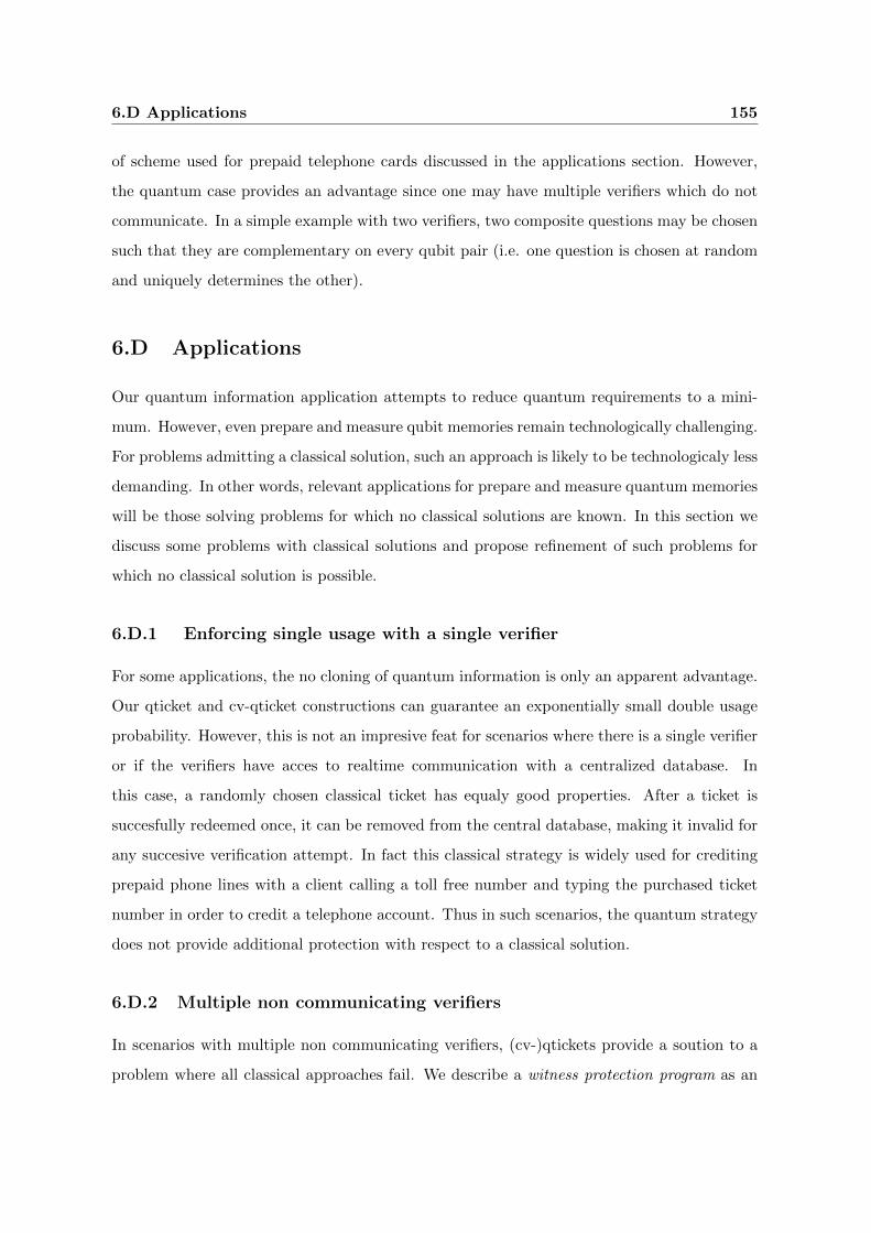
6.D Applications 155
of scheme used for prepaid telephone cards discussed in the applications section. However,
the quantum case provides an advantage since one may have multiple verifiers which do not
communicate. In a simple example with two verifiers, two composite questions may be chosen
such that they are complementary on every qubit pair (i.e. one question is chosen at random
and uniquely determines the other).
6.D Applications
Our quantum information application attempts to reduce quantum requirements to a mini-
mum. However, even prepare and measure qubit memories remain technologically challenging.
For problems admitting a classical solution, such an approach is likely to be technologicaly less
demanding. In other words, relevant applications for prepare and measure quantum memories
will be those solving problems for which no classical solutions are known. In this section we
discuss some problems with classical solutions and propose refinement of such problems for
which no classical solution is possible.
6.D.1 Enforcing single usage with a single verifier
For some applications, the no cloning of quantum information is only an apparent advantage.
Our qticket and cv-qticket constructions can guarantee an exponentially small double usage
probability. However, this is not an impresive feat for scenarios where there is a single verifier
or if the verifiers have acces to realtime communication with a centralized database. In
this case, a randomly chosen classical ticket has equaly good properties. After a ticket is
succesfully redeemed once, it can be removed from the central database, making it invalid for
any succesive verification attempt. In fact this classical strategy is widely used for crediting
prepaid phone lines with a client calling a toll free number and typing the purchased ticket
number in order to credit a telephone account. Thus in such scenarios, the quantum strategy
does not provide additional protection with respect to a classical solution.
6.D.2 Multiple non communicating verifiers
In scenarios with multiple non communicating verifiers, (cv-)qtickets provide a soution to a
problem where all classical approaches fail. We describe a witness protection program as an
156 6. Unforgeable noise-tolerant quantum tokens
example of how such a scenario might look like.
In a witness protection program, a governmental institution decides to give asylum to a
key eye witness to whom an unforgeable quantum token is issued. This token can be used
by the witness (holder) to claim asylum in any of a set of participating hotels (verifiers).
The issuer also provides all hotels with the necessary information to verify the tokens. When
using the token, neither the eye-witness nor the chosen hotel wish to divulge the locale where
the witness is hosted, thus protecting both from being targets of an attack. This includes
suspending communication between participating hotels as well as with the issuing authority.
Any classical solution can not prevent a sufficiently resourceful holder from making copies of
the received token, thus hotels are forced to communicate in order to avoid its double use.
In this case, a quantum solution based on unforgeable tokens is the sole possibility to satisfy
these unique constraints.
Figure 6.5: 1) The issuing entity hands a qticket to the key witness. 2) It provides the hotels
with the secret classical description which will be used to verify it. 3a) An honest witness
choses a hotel and physically transfer the qticket for verification. It will be accepted as long
as the level of accumulated noise is below threshold. 3b) A dishonest witness will fail to
counterfeit his/her qticker to provide acomodation for an additional guest. However, there is
no way of avoiding a valid qticket from changing hands.
6.D.3 Reduced availability under sporadic verification
In principle, a centralized database may guarante that classical ticket are only redeemed
once. However, there are situations where the ticket should be available only to one holder
at a time and the non-clonable nature of a qticket allows enforcing this. One such example is

6.D Applications 157
the sporadic control of tickets required for a given service. For concreteness, imagine a qticket
which is valid for making use of a public transportation network. Commuters are sporadically
controled, at which point if they are found to have a invalid qticket they are charged an
important fine, whereas if they are found to hold a valid qticket, they are provided with a
fresh substitute. If the transportation tickets are classical, sporadic control can not avoid
counterfeited copies in the hands of coluding commuters from circulating simultaneously.
The deceiving commuters need only communicate classicaly among each other before and
after they are controled, effectively sharing a single classical ticket to make use of the service
multiple times1. In contrast the unavailability of long distance quantum comunication would
disallows them to share a qticket in such a way (i.e. each valid qticket may only be at one
place at a time).
6.D.4 The quantum credit card
Having developed a single verification, noise tolerant, non-forgeable token, such as the cv-
qticket, it is now possible to examine generalizations to interesting composite protocols. For
instance, Gavinsky’s proposal[44] allows for multiple verification rounds to be performed on
a single token, while also ensuring that the token can not be split into two independently
valid subparts. Such a construction may be seen as a quantum credit card. Indeed, the
classical communication which takes place with the issuer (bank) to verify the cv-qticket
(via “challenge” questions) may be intentionally publicized to a merchant who needs to be
convinced of the card’s validity. An alternate possibility is to follow the original interpretation
as a quantum cash token where verification is performed by the receiver each time the “money”
changes hands.
6.D.5 Excluding eavesdropers
While qtickets do not provide additional advantage against dishonest holder in the scenario of
a single verifier quantumness may provide an advantage against eavesdroping and untrusted
communication. In order to make online banking more secure, Banks routinely use TANs
(transaction authentication numbers) as an additional security measure. The bank sends its
client a list of TANs via postal service in addition to an online password which is set up via
1If the classical ticket is not renewed upon control even communication is unnecesary.
158 6. Unforgeable noise-tolerant quantum tokens
another channel. Each time a bank transaction is requested online by the client, the bank
requests a TAN from the list to guarantee the authenticity of the transaction. An impostor
then needs to know both a secret password used by the user and some TANs, thus increasing
the difficulty to succesfully impersonate a transaction with respect to any single security
measure. However, since TANs are classical objects it is conceivable that an eavesdroper may
learn them while remaining undetected (imagine an eavesdroper taking xray pictures of the
correspondence). This means that with some effort of the eavesdroper the additional security
measure becomes ineffective.
This problem can be straightforwardly resolved by using quantum prepare and measure
memories. Even if a cv-qticket is sent via an untrusted optical fiber or postal service, the
receiver may openly communicate with the issuer and sacrifice some of the received qubits in
order to obtain a bound on how much information could have leaked to eavesdropers. This is
precisely the approach taken in QKD to obtain a statistical bound on the information that has
leaked out. Gavinsky’s Q scheme, allowing multiple verification rounds may be reinterpreted
as quantum TAN lists. The holder of a quantum TAN list may verify its validity, and perform
a transaction by publicly communicating with the bank. If the quantum TAN list is verified
to be legitimate, then the probability of an eavesdroper getting verified by using the leaked
information will be negligible (exponentially small). In turn, the cv-qtickets described in
the main text and appendix may be used as basic building blocks for such a scheme in the
presence of noise.

References
[1] S. Aaronson: Quantum Copy-Protection and Quantum Money, In 24th Annual IEEE
Conference on Computational Complexity, 2009.. IEEE (July 2009) pages 229–242.
[2] V.M. Acosta, E. Bauch, M.P. Ledbetter, A. Waxman, L. Bouchard and D. Budker,
Phys. Rev. Lett. 104 (2010), 070801.
[3] D. Aharonov and M. Ben-Or, quant-ph/9611025 (1996).
[4] D. Aharonov, M. Ben-Or, R. Impagliazzo and N. Nisan, quant-ph/9611028 (1996).
[5] C. Ahn, A.C. Doherty and A.J. Landahl, Phys. Rev. A 65 (2002), 042301.
[6] C.S. Ahn: Extending quantum error correction: new continuous measurement protocols
and improved fault-tolerant overhead. Pasadena, CA, Caltech, Dissertation, 2004.
[7] R. Alicki and M. Fannes, Phys. Rev. A 79 (2009), 012316.
[8] R. Alicki, M. Fannes and M. Horodecki, arXiv:0810.4584 (2008).
[9] R. Alicki, M. Horodecki, P. Horodecki and R. Horodecki, arXiv:0811.0033 (2008).
[10] P.W. Anderson, Phys. Rev. Lett. 18 (1967), 1049.
[11] D. Bacon, Phys. Rev. A 73 (2006), 012340.
[12] D. Bacon, Phys. Rev. A 78 (2008), 042324.
[13] M.V. Balabas, T. Karaulanov, M.P. Ledbetter and D. Budker, Phys. Rev. Lett. 105
(2010), 070801.

160 REFERENCES
[14] G. Balasubramanian, P. Neumann, D. Twitchen, M. Markham, R. Kolesov,
N. Mizuochi, J. Isoya, J. Achard, J. Beck, J. Tissler, V. Jacques, P.R. Hemmer,
F. Jelezko and J. Wrachtrup, Nat. Materials 8 (2009), 383.
[15] P. Benioff, Journal of Statistical Physics 29 (1982), 515.
[16] C.H. Bennet and G. Brassard: Quantum Cryptography: Public Key Distribution and
Coin Tossing, In Proceedings of the IEEE International Conference on Computers,
Systems & Signal Processing, Bangalore, India. IEEE, New York (1984) pages 175–
179.
[17] C.H. Bennett, IBM Journal of Research and Development 17 (1973), 525.
[18] K. Binder and E. Stoll, Phys. Rev. Lett. 31 (1973), 47.
[19] S. Bravyi, D.P. DiVincenzo, D. Loss and B.M. Terhal, Phys. Rev. Lett. 101 (2008),
070503.
[20] S. Bravyi and M.B. Hastings, arXiv:1001.4363 (2010).
[21] S. Bravyi, M.B. Hastings and S. Michalakis, Jour. Math. Phys. 51 (2010), 093512.
[22] S. Bravyi and B. Terhal, New Jour. Phys. 11 (2009), 043029.
[23] K.R. Brown, Phys. Rev. A 76 (2007), 022327.
[24] D. Bruss, M. Cinchetti, G. Mauro D’Ariano and C. Macchiavello, Phys. Rev. A 62
(2000), 012302.
[25] H.J. Carmichael: Statistical Methods in Quantum Optics 1: Master Equations and
Fokker-Planck Equations (Theoretical and Mathematical Physics). Springer, November
1998.
[26] S. Chesi, D. Loss, S. Bravyi and B.M. Terhal, New Jour. Phys. 12 (2010), 025013.
[27] S. Chesi, B. Rothlisberger and D. Loss, arXiv:0908.4264 (2009).
[28] A.M. Childs and W. van Dam, arXiv:0812.0380 (2008).
[29] M. Christandl, N. Datta, A. Ekert and A.J. Landahl, Phys. Rev. Lett. 92 (2004), 187902.
REFERENCES 161
[30] E. Cirillo and J. Lebowitz, Jour. Stat. Phys. 90 (1998), 211.
[31] C. Cohen-Tannoudji, J. Dupont-Roc and G. Grynberg: AtomPhoton Interactions: Ba-
sic Processes and Applications. 1. ed. Wiley-Interscience, March 1992.
[32] E. Dennis, A. Kitaev, A. Landahl and J. Preskill, Jour. Math. Phys. 43 (2002), 4452.
[33] D. Deutsch, Proceedings of the Royal Society A Mathematical Physical and Engineering
Sciences 400 (1985), 97.
[34] S. Diehl, A. Micheli, A. Kantian, B. Kraus, H.P. Bchler and P. Zoller, Nature Phys. 4
(2008), 878.
[35] L. Duan and C. Monroe, Rev. Math. Phys. 82 (2010), 1209.
[36] M.V.G. Dutt, L. Childress, L. Jiang, E. Togan, J. Maze, F. Jelezko, A.S. Zibrov,
P.R. Hemmer and M.D. Lukin, Science 316 (2007), 1312 .
[37] A.K. Ekert, Phys. Rev. Lett. 67 (1991), 661.
[38] E. Farhi, D. Gosset, A. Hassidim, A. Lutomirski, D. Nagaj and P. Shor, Phys. Rev.
Lett. 105 (2010), 190503.
[39] E. Farhi, D. Gosset, A. Hassidim, A. Lutomirski and P. Shor, arXiv:1004.5127 (2010).
[40] R.P. Feynman, International Journal of Theoretical Physics 21 (1982), 467.
[41] P. Gacs, Jour. Stat. Phys. 103 (2001), 45.
[42] A. Gali, Phys. Rev. B 79 (2009), 235210.
[43] A. Gali, M. Fyta and E. Kaxiras, Phys. Rev. B 77 (2008), 155206.
[44] D. Gavinsky, arXiv:1109.0372 (2011).
[45] N. Gisin, G. Ribordy, W. Tittel and H. Zbinden, Rev. Math. Phys. 74 (2002), 145.
[46] S. Gladchenko, D. Olaya, E. Dupont-Ferrier, B. Doucot, L.B. Ioffe and M.E. Gershenson,
Nature Phys. 5 (2009), 48.
[47] D. Gottesman, Phys. Rev. A 57 (1998), 127.
162 REFERENCES
[48] D. Gottesman, arXiv:0904.2557 (2009).
[49] D. Gottesman and H. Lo, IEEE Transactions on Information Theory 49 (2003), 457.
[50] L.F. Gray. In Perplexing Problems in Probability, 1. ed. Birkhauser Verlag AG (August
1999), pages 331–354.
[51] G. Grinstein, IBM J. Res. & Dev. 48 (2004).
[52] G. Gutoski and J. Watrous: Toward a general theory of quantum games, In Proceedings
of the thirty-ninth annual ACM symposium on Theory of computingSTOC ’07. ACM,
New York, NY, USA (2007) page 565?574.
[53] A. Hamma, C. Castelnovo and C. Chamon, Phys. Rev. B 79 (2009), 245122.
[54] A. Hamma and D.A. Lidar, Phys. Rev. Lett. 100 (2008), 030502.
[55] J.W. Harrington: Analysis of quantum error-correcting codes: symplectic lattice codes
and toric codes. Caltech, Thesis, 2004.
[56] A.W. Harrow, A. Hassidim and S. Lloyd, Phys. Rev. Lett. 103 (2009), 150502.
[57] M.B. Hastings and X.G. Wen, Phys. Rev. B 72 (2005), 045141.
[58] W. Hoeffding, Journal of the American Statistical Association 58 (1963), 13.
[59] M. Horodecki, P.W. Shor and M.B. Ruskai, Rev. Math. Phys. 15 (2003), 629.
[60] D.B. Hume, T. Rosenband and D.J. Wineland, Phys. Rev. Lett. 99 (2007), 120502.
[61] R. Impagliazzo and V. Kabanets. Constructive Proofs of Concentration Bounds. Tech-
nical report 072, Electronic Colloquium on Computational Complexity, 2010.
[62] V. Jacques, P. Neumann, J. Beck, M. Markham, D. Twitchen, J. Meijer, F. Kaiser,
G. Balasubramanian, F. Jelezko and J. Wrachtrup, Phys. Rev. Lett. 102 (2009), 7.
[63] L. Jiang, M.V.G. Dutt, E. Togan, L. Childress, P. Cappellaro, J.M. Taylor and
M.D. Lukin, Phys. Rev. Lett. 100 (2008), 073001.
[64] S.P. Jordan and E. Farhi, Phys. Rev. A 77 (2008), 062329.
REFERENCES 163
[65] S.P. Jordan, E. Farhi and P.W. Shor, Phys. Rev. A 74 (2006), 052322.
[66] P. Karbach, Phys. Rev. A 72 (2005), 030301.
[67] A. Kay, Phys. Rev. Lett. 102 (2009), 070503.
[68] A. Kay, arXiv:0903.4274 (2009).
[69] A. Kay and R. Colbeck, arXiv:0810.3557 (2008).
[70] A. Kay and M. Ericsson, New Jour. Phys. 7 (2005), 143.
[71] N. Khaneja, R. Brockett and S.J. Glaser, Phys. Rev. A 63 (2001), 032308.
[72] C. King, Information Theory, IEEE Transactions on 49 (2003), 221.
[73] A.Y. Kitaev, Physics-Uspekhi 44 (2001), 131.
[74] A.Y. Kitaev, Annals of Physics 303 (2003), 2.
[75] E. Knill, R. Laflamme and W.H. Zurek, Science 279 (1998), 342.
[76] H. Krauter, C.A. Muschik, K. Jensen, W. Wasilewski, J.M. Petersen, J.I. Cirac and
E.S. Polzik, Phys. Rev. Lett. 107 (2011), 080503.
[77] D. Kribs, R. Laflamme and D. Poulin, Phys. Rev. Lett. 94 (2005), 180501.
[78] C. Kurtsiefer, S. Mayer, P. Zarda and H. Weinfurter, Phys. Rev. Lett. 85 (2000), 290.
[79] T.D. Ladd, D. Maryenko, Y. Yamamoto, E. Abe and K.M. Itoh, Phys. Rev. B 71
(2005), 014401.
[80] R. Laflamme, C. Miquel, J.P. Paz and W.H. Zurek, Phys. Rev. Lett. 77 (1996), 198.
[81] C. Langer, R. Ozeri, J.D. Jost, J. Chiaverini, B. DeMarco, A. Ben-Kish, R.B. Blakestad,
J. Britton, D.B. Hume, W.M. Itano, D. Leibfried, R. Reichle, T. Rosenband, T. Schaetz,
P.O. Schmidt and D.J. Wineland, Phys. Rev. Lett. 95 (2005), 060502.
[82] D.A. Lidar, Phys. Rev. Lett. 100 (2008), 160506.
[83] E.H. Lieb and D.W. Robinson, Comm. Math. Phys. 28 (1972), 251.
164 REFERENCES
[84] G. Lindblad, Comm. Math. Phys. 48 (1976), 119.
[85] A. Lutomirski, arXiv:1107.0321 (2011).
[86] A. Lutomirski, S. Aaronson, E. Farhi, D. Gosset, A. Hassidim, J. Kelner and P. Shor,
arXiv:0912.3825 (2009).
[87] H. Mabuchi, New Jour. Phys. 11 (2009), 105044.
[88] N.B. Manson, J.P. Harrison and M.J. Sellars, Physical Review B 74 (2006), 104303.
[89] S. Massar and S. Popescu, Phys. Rev. Lett. 74 (1995), 1259.
[90] P.C. Maurer, G. Kucsko, C. Latta, L. Jiang, N.Y. Yao, S.D. Bennett, F. Pastawski,
D. Hunger, N. Chisholm, M. Markham, D.J. Twitchen, J.I. Cirac and M.D. Lukin,
Science 336 (2012), 1283.
[91] M. Mehring: Principles of High Resolution Nmr in Solids. 2. ed. Springer-Verlag,
February 1983.
[92] G.E. Moore, Electronics 38 (1965), 2005.
[93] J.J.L. Morton, A.M. Tyryshkin, R.M. Brown, S. Shankar, B.W. Lovett, A. Ardavan,
T. Schenkel, E.E. Haller, J.W. Ager and S.A. Lyon, Nature 455 (2008), 1085.
[94] M. Mosca and D. Stebila, arXiv:0911.1295 (2009).
[95] P. Neumann, J. Beck, M. Steiner, F. Rempp, H. Fedder, P.R. Hemmer, J. Wrachtrup
and F. Jelezko, Science 329 (2010), 542 .
[96] P. Neumann, R. Kolesov, V. Jacques, J. Beck, J. Tisler, A. Batalov, L. Rogers,
N.B. Manson, G. Balasubramanian, F. Jelezko and J. Wrachtrup, New Journal of
Physics 11 (2009), 013017.
[97] P. Neumann, R. Kolesov, B. Naydenov, J. Beck, F. Rempp, M. Steiner, V. Jacques,
G. Balasubramanian, M.L. Markham, D.J. Twitchen, S. Pezzagna, J. Meijer,
J. Twamley, F. Jelezko and J. Wrachtrup, Nature Phys. 6 (2010), 249.
[98] M.A. Nielsen, Phys. Lett. A 303 (2002), 249.
REFERENCES 165
[99] Z. Nussinov and G. Ortiz, Phys. Rev. B 77 (2008).
[100] Z. Nussinov and G. Ortiz, Ann. of Phys. 324 (2009), 977.
[101] O. Oreshkov and T.A. Brun, Phys. Rev. A 76 (2007), 022318.
[102] A. Panconesi and A. Srinivasan, SIAM Journal on Computing 26 (1997), 350.
[103] F. Pastawski, A. Kay, N. Schuch and I. Cirac, Phys. Rev. Lett. 103 (2009), 080501.
[104] F. Pastawski, A. Kay, N. Schuch and I. Cirac, Quant. Inform. and Comp. 10 (2010),
0580.
[105] J.P. Paz and W.H. Zurek, Proc. R. Soc. A 454 (1998), 355.
[106] H.L. Richards, S.W. Sides, M.A. Novotny and P.A. Rikvold, J. Magn. Magn. Mater.
150 (1995), 37.
[107] R.L. Rivest, A. Shamir and L. Adleman, Communications of the ACM 21 (1978), 120.
[108] T. van der Sar, Z.H. Wang, M.S. Blok, H. Bernien, T.H. Taminiau, D.M. Toyli, D.A. Li-
dar, D.D. Awschalom, R. Hanson and V.V. Dobrovitski, Nature 484 (2012), 82.
[109] M. Sarovar and G.J. Milburn, Phys. Rev. A 72 (2005), 012306.
[110] V. Scarani and R. Renner, Phys. Rev. Lett. 100 (2008), 200501.
[111] P. Shor: Fault-tolerant quantum computation, In Proceedings of the 37th Annual Sympo-
sium on Fundamentals of Computer Science. IEEE Computer Society Press, Burlington,
VT, USA (1996) pages 56–65.
[112] P.W. Shor, Proceedings 35th Annual Symposium on Foundations of Computer Science
35 (1994), 124.
[113] P.W. Shor, Phys. Rev. A 52 (1995), R2493.
[114] P.W. Shor, SIAM J. Comput. 26 (1997), 1484.
[115] P. Spinicelli, A. Drau, L. Rondin, F. Silva, J. Achard, S. Xavier, S. Bansropun, T. De-
buisschert, S. Pezzagna, J. Meijer, V. Jacques and J. Roch, New Jour. Phys. 13 (2011),
025014.
166 REFERENCES
[116] M. Steiner, P. Neumann, J. Beck, F. Jelezko and J. Wrachtrup, Phys. Rev. B 81 (2010),
035205.
[117] C.J. Terblanche, E.C. Reynhardt and J.A. van Wyk, Solid State Nuclear Magnetic
Resonance 20 (2001), 1. PMID: 11529416.
[118] E. Togan, Y. Chu, A.S. Trifonov, L. Jiang, J. Maze, L. Childress, M.V.G. Dutt,
A.S. Sorensen, P.R. Hemmer, A.S. Zibrov and M.D. Lukin, Nature 466 (2010), 730.
[119] A. Toom, Problems of Information Transmission 10 (1974), 239.
[120] D.M. Toyli, C.D. Weis, G.D. Fuchs, T. Schenkel and D.D. Awschalom, Nano Lett. 10
(2010), 3168.
[121] A.M. Tyryshkin, S. Tojo, J.J.L. Morton, H. Riemann, N.V. Abrosimov, P. Becker,
H. Pohl, T. Schenkel, M.L.W. Thewalt, K.M. Itoh and S.A. Lyon, Nat. Materials ad-
vance online publication (2011).
[122] P. Vaidya: Geometry helps in matching, In Proceedings of the twentieth annual ACM
symposium on Theory of computingSTOCS. ACM (1988) pages 422–425.
[123] L.M.K. Vandersypen and I.L. Chuang, Rev. Math. Phys. 76 (2005), 1037.
[124] L.C. Venuti and P. Zanardi, Phys. Rev. Lett. 99 (2007), 095701.
[125] F. Verstraete, M.M. Wolf and J.I. Cirac, Nature Phys. 5 (2009), 633.
[126] G. Waldherr, J. Beck, M. Steiner, P. Neumann, A. Gali, T. Frauenheim, F. Jelezko and
J. Wrachtrup, Phys. Rev. Lett. 106 (2011), 157601.
[127] G. Wendin, Proc. R. Soc. A 361 (2003), 1323 .
[128] R.F. Werner, Phys. Rev. A 58 (1998), 1827.
[129] S. Wiesner, ACM SIGACT News 15 (1983), 78.
[130] M.M. Wolf, Nature Phys. 4 (2008), 834.
[131] N.Y. Yao, L. Jiang, A.V. Gorshkov, P.C. Maurer, G. Giedke, J.I. Cirac and M.D. Lukin,
arXiv:1012.2864 (2010).
167
[132] H. Zhu and B. Englert, Phys. Rev. A 84 (2011), 022327.

168

List of Figures
2.1 Decoding a nested QECC. The “discarded” qubits carry most of the entropy
and are not used further. . . . . . . . . . . . . . . . . . . . . . . . . . . . . . 13
2.2 A step-like trajectory in green illustrates the two ways of leaving region (2.7)
of good trajectories (dashed lines): either a spin flip can take the polarization
out of the marked region (thick blue), or polarization may leave region (2.7)
as time passes without a spin flip (red dots). . . . . . . . . . . . . . . . . . . 15
3.1 Two hollow dots indicate positions where a pair of vertex anyons may be created
by U† and/or by U with probability p. Anyons created by U† are propagated
by P along the darkening path. A table is provided indicating the probability
of possible error configurations and their corresponding syndrome observables
(1 (0) representing anyon presence (absence)). . . . . . . . . . . . . . . . . . . 42
3.2 Anyon pairs corresponding to each thick red edge may be created by U†. After
a time tf , the right anyon from each pair introduced will be propagated a
distance 4S + 2 to the right introducing Z errors along the darkening paths.
Finally, U acting on the same red segment may move an unpropagated anyon
one position to the right or create a neighboring anyon pair on it. The number
of big steps (or equivalently of crossings) during the upward propagation is
given by S, which in the case of the figure is 2. . . . . . . . . . . . . . . . . . 45
3.3 The average probability of error for L1 correction after the system evolves for a
time tf under the described Hamiltonian perturbation. Here, anyon pairs arise,
and evolve to distances of d20 ln(N)e, with a probability of 10%, all collinear on
a line of length N . Each point represents an average over 106 random samples,
with error bars representing the magnitude of estimated statistical errors. . . 48
170 LIST OF FIGURES
3.4 There is an energy gap γ separating the eigenenergies corresponding to an ex-
ponentially small subspace P0 from the energies of the Hamiltonian eigenstates
giving rise to the rest of the Hilbert space. . . . . . . . . . . . . . . . . . . . . 62
3.5 Each edge in the grid represents a physical qubit and opposite sides of the grid
are identified by toric periodic boundary conditions. Typical plaquette and
vertex operators are depicted near the center. Two vertical loop operators, X1
and Z2, which allow breaking the degeneracy are also presented. One can take
these to be the X and Z operators for the first and second logically encoded
qubits respectively. The complementary (anticommuting) operators are given
by analogous horizontal loops. . . . . . . . . . . . . . . . . . . . . . . . . . . 65
3.6 Illustration of a possible configuration of three vertex anyon pairs (small cir-
cles). Segments indicate possible qubits where Z rotations could be introduced
in order to remove the anyons. Solid and dotted segments illustrate the anyon
matching arising from l1-EC and l∞-EC respectively. Since together they com-
plete a non-trivial loop, the matchings are logically inequivalent. . . . . . . . 66
3.7 In an N × N lattice, there are two sets of N/k rows (k ∼ O(1)) and two
sets of columns and rows, each of which corresponds to the construction of
(Sec. 3.4.2) for a different error type (X1, Z2 are introduced by columns starting
at horizontal stripes and Z1 and X2 are introduced by rows starting from
vertical stripes). . . . . . . . . . . . . . . . . . . . . . . . . . . . . . . . . . . 69
4.1 We assume that a piece of quantum information is encoded into a many body
system. The engineered dissipation, is then responsible for making the degrees
of freedom which carry the encoded quantum information resilient against the
uncontrolled noise processes taking place. Finally, the decoding process ex-
tracts the quantum information from the collective degrees of freedom. . . . . 74

LIST OF FIGURES 171
4.2 The mean time to error for a logical observable is plotted in log scale units
of 1Γ . Error rates Γε are provided in units of Γ. The plots further suggests
the existence of a critical value for error rates Γ?ε ≈ 0.004. (a) Each curve
corresponds to a fixed odd value of the lattice size N . The independent axis
Γε/Γ is also in log scale suggesting that for each fixed N the information
lifetime show an asymptotic (small Γε) power law dependence with 1/Γε with
the exponent increasing for larger N . (b) Each curve corresponds to a fixed
value of the error rate Γε. For low error rates Γε < Γ?ε, lifetime is seen to
improve exponentially with N . . . . . . . . . . . . . . . . . . . . . . . . . . . 79
4.3 Relaxation time for ZEC (red curves) and XL (blue curves) in units of Γ−1.
Each red curve presents the relaxation time τZ (numerically obtained) cor-
responding to one value of the relative dephasing rate Γ/Γphase given by the
intercept at N = 1. Blue curve have the functional form τX = Γ−1dep ∗N−2 and
each corresponds to one value of Γ/Γdep also given by the intercept at N = 1.
The lifetime τ of the encoded logical qubit can be seen to be estimated by
τ ≈ min{τX , τZ}. Given Γ/Γdep and Γ/Γphase, one may intersect the corre-
sponding curves to obtain the value of N leading to the optimal qubit lifetime
τ . For example, if Γdep = 5× 10⁻⁵Γ and Γphase = 0.1Γ the optimal lattice size
of 4× 4 allows a ×100 increase in the quantum information relaxation time τ .
A more extreme case may be seen when Γphase = 0.01Γ and Γdep ≤ 5× 10⁻⁵Γ
where a factor ×50 is gained by simply using a 2× 2 lattice. . . . . . . . . . 82
4.4 Recovery probability of an encoded observable in the 4D toric code is plotted as
a function of depolarization probability per qubit. Odd lattices sizes from 1 to
11 are represented in the different curves and suggest a critical depolarization
probability of approximately 7.5%. . . . . . . . . . . . . . . . . . . . . . . . 90

172 LIST OF FIGURES
5.1 a) An NV-center is obtained by removing two nearest neighbour carbons in
the diamond lattice and replacing one of them by a nitrogen atom (light grey)
while keeping the lattice location vacant (blue). In practice, a way to fabri-
cate these centers is via high temperature annealing of natural or implanted
nitrogen impurities until they become attached to a vacancy. b) Schematic
level diagram for an NV center (left box) and a 13C nuclear spin (right box)
under illumination with green laser light. The green arrows indicate optical
transitions addressed by our green laser pulse, red arrows show electronic decay
and blue arrows indicate depolarization of the electronic spin. The transition
rates for NV are taken from [88] with the decay rate from the electronic ex-
cited state to the ground state γ = 113ns , the decay rate from the singlet to
ms = 0 of the electronic ground state Γ = 1300ns and the decay rate from the
electronic excited states with ms = ±1 to the singlet γb = 0.3γ. Moreover we
assumed the decay rate of the excited state of NV0 to be on the same order as
for NV. The deionization rate from NV to NV0 is taken to be γ1 = I/Isat70ns and
the ionization rate γ2 = 2γ1 [126]. The depolarization time for the electronic
spin for NV is taken to be TNV−
1e = 8ms and for the case of NV0, TNV0
1e = 6µs
[126]. All the remaining rates are taken to be zero. Reprinted from Science
336 (2012) 1283-1286 with permission from AAAS. . . . . . . . . . . . . . . 103
5.2 The |ms = ±1〉 excited states decay into the singlet shelve state with a rate
γb ≈ 0.3γ which in turn decays mainly into the |ms = 0〉 ground state at a
slower rate Γ ≈ 1300ns . No photons are emitted during the time spent in the
shelf state leading to a lower initial fluorescence intensity for the |ms = ±1〉states. Eventually, the electronic spin becomes polarized into the |ms = 0〉independent of the initial state. Such a 1/e decay occurs on a time scale of the
order of 150ns and steady state polarization can be assumed after 1µs (these
rates depend on the strength of the optical driving). . . . . . . . . . . . . . . 109
LIST OF FIGURES 173
5.3 Nuclear 13C qubit readout. a) Circuit diagram of repetitive readout of the
nuclear spin |n〉. The readout uses a CnNOTe gate consisting of multiple rep-
etitions of an electronic spin Ramsey sequence and subsequent repolarization.
Many repetitions are needed to accumulate the small amounts of information
provided by each measurement attempt. b) Fluorescence time trace showing
single shot readout of the nuclear spin and corresponding quantum jumps.
The integration time for a single point is 4.4 s. c) Histogram of continuous
repetitive readouts (20000 in 4.4 s) showing two overlapping distributions of
fluorescence photon counts corresponding to nuclear spin states: | ↓〉 (blue) and
| ↑〉 (red). d) Nuclear spin orientation lifetime, T1n as a function of 532 nm
laser power. As shown in the inset, each data point is extracted from a series of
two repetitive readout sequences, the first one corresponding to initialization
and the second to measurement. The solid red curve represents the theoreti-
cal prediction from the simple model of nuclear depolarization induced by the
off-axis dipolar hyperfine field. Reprinted from Science 336 (2012) 1283-1286
with permission from AAAS. . . . . . . . . . . . . . . . . . . . . . . . . . . . 111
5.4 Photon count statistics and initialization fidelity a) The number of events as-
sociated to a given number of detected photons is plotted in a histogram (blue)
after initialization of the nuclear spin in |↓〉 (green) and |↑〉 (red) and 10000
repetitive readouts (2.2s). The solid curves correspond to a theoretical fit ac-
counting for the effect of a possible nuclear spin flips on the ideally Gaussian
distributions. The green and red regions indicate photon count numbers for
which initialization is assumed in the |↓〉 respectively |↑〉 nuclear states. b)
The green and red curves indicate the initialization fidelity of |↓〉 respectively
|↑〉 nuclear states as a function of the count threshold taken. Stricter count
thresholds lead to higher fidelity but to discarding a larger fraction of initializa-
tions with the net effect of prolonging the effective initialization time required.
Reprinted from Science 336 (2012) 1283-1286 with permission from AAAS. . 112

174 LIST OF FIGURES
5.5 Decoupling pulse sequences The WHH sequence is capable of achieving
dipole dipole decoupling with only 4 π/2 pulses each applied around the indi-
cated axis. The MREV-8 has the same averaging effect as WHH for the dipole
dipole coupling but shows a higher robustness to RF pulse errors. Finally,
CPMG/MREV sequence includes additional π pulses to compensate external
magnetic fields. Reprinted from Science 336 (2012) 1283-1286 with permission
from AAAS. . . . . . . . . . . . . . . . . . . . . . . . . . . . . . . . . . . . . 118
5.6 Combined dephasing from detuning and dipole-dipole interactions 120
5.7 Experimental coherence extension a) Experimental sequence used to measure
the nuclear coherence time. A modified Mansfield Rhim Elleman Vaughan
(MREV) decoupling sequence [79] is utilized. It consists of 16 MREV-8 pulse
trains interwoven with 8 phase-refocusing π-pulses. Each MREV-8 pulse se-
quence can be achieved through π/2 rotations around four different axes. b)
Nuclear coherence as a function of green laser power. Red data constitute a
measurement of T2n using a nuclear spin echo; blue data T2n contain the addi-
tional MREV sequence. The dashed fits are calculated from the spin-fluctuator
model. Reprinted from Science 336 (2012) 1283-1286 with permission from
AAAS. . . . . . . . . . . . . . . . . . . . . . . . . . . . . . . . . . . . . . . . 121
6.1 a) Depicts the pigeonhole type argument which is utilized in the proof of qticket
soundness. For a tolerance fidelity Ftol, a qticket is only successfully authen-
ticated if it contains at least FtolN valid qubits. However, for two counterfeit
qtickets, not all valid qubits must coincide. The minimum number of perfectly
cloned qubits enabling both qtickets to be accepted is, (2Ftol − 1)N . b) De-
picts the quantum retrieval type situation envisioned for cv-qtickets. For two
verifiers asking complementary “challenge” questions, the optimal strategy is
for the user to measure in an intermediate basis. Such a strategy saturates the
tolerance threshold, F cvtol = 1+1/
√2
2 . . . . . . . . . . . . . . . . . . . . . . . . . 126
LIST OF FIGURES 175
6.2 a) Depicts the possibility of using the cv-qticket framework to implement a
quantum-protected credit card. Unlike its classical counterpart, the quantum
credit card would naturally be unforgeable; this prevents thieves from being
able to simply copy credit card information and perform remote purchases. b)
Depicts a dishonest user who attempts to copy a concert qticket (e.g. same
serial number), enabling his friend to enter at an alternate checkpoint gate.
Naively, each verifier can communicate with one another to prevent such abu-
sive ticket cloning. However, such a safeguard can be overcome in the event
that the communication among verifiers is either unsecured, unavailable or sev-
ered (possibly by the dishonest user himself). The qticket is exempt from this
type of attack since security is guaranteed even in the case of isolated verifiers. 130
6.3 a) We schematically illustrate how a dynamical strategy S works. Each step of
a strategy (grey rectangles) is a CPTP map S~b which depends on the classical
outcome ~b of previous verifications. The first map S∅ takes an original qticket
ρ as input, whereas subsequent steps rely on an internal memory state of the
holder. The content of internal memory could range from no information at
all, to a full original qticket and a detailed register of previous submissions.
The verifiers have a fixed strategy Πρ which consists of applying the mea-
surement {P ρacc, Pρrej} and only returning the classical boolean measurement
outcome. b) By fixing the classical input ~b to the strategy, a CPTP map
S~b ∈ HQ → H⊗ len(~b)+1Q ⊗ HH is constructed, corresponding to one possible
partial application of the strategy S. This CPTP map produces len(~b) + 1
possibly entangled outputs in HQ from a single input qticket. . . . . . . . . 140
6.4 We numerically calculate the probability of accepting two copies of a qticket
when the adversary strategy is assumed to be independently cloning each of
the N qubits using an optimal cloning map. We see that the probability of
producing two accepted qtickets approaches a step function at 5/6 with N . . 142

176
6.5 1) The issuing entity hands a qticket to the key witness. 2) It provides the ho-
tels with the secret classical description which will be used to verify it. 3a) An
honest witness choses a hotel and physically transfer the qticket for verification.
It will be accepted as long as the level of accumulated noise is below thresh-
old. 3b) A dishonest witness will fail to counterfeit his/her qticker to provide
acomodation for an additional guest. However, there is no way of avoiding a
valid qticket from changing hands. . . . . . . . . . . . . . . . . . . . . . . . . 156
Acknowledgements
I am greatly indebted to my supervisor, Ignacio Cirac, for proposing exciting research pro-
grams and providing the appropriate environment to carry them out. Throughout these years
he has been very generous in providing time for discussion and guidance, while also offering
me the freedom to develop my scientific independence.
I would like to thank Alastair Kay, Norbert Schuch, Lucas Clemente, Peter Maurer, Georg
Kucsko, Norman Yao, Liang Jiang and Mikhail Lukin for their fruitful and constructive
collaboration on the different research projects pursued during this thesis.
I also would like to acknowledge the people who have been especially generous with their
guidance. Miguel Aguado, was a true mentor and introduced me to the notions required for
understanding the topological approach to quantum memory and computing. Eric Kessler has
provided invaluable help in guiding my dive into the literature of Nitrogen Vacancy centres.
I should also thank, Geza Giedke, Mari Carmen Banuls, Maarten van den Nest and Thomas
Schulte-Herbruggen for their valuable advice and stimulating discussion.
Special thanks go to Heike and Anika without whom this thesis would be lost in trans-
lation. Thank you for always bringing good mood into the office and for the good advice. I
would also like to thank, Leonardo, Oriol, Gemma, Matteo, Martin Schutz, Bierger, Tassilo,
Sebastien, Michael, Oliver and the rest of my colleagues and friends at MPQ for their com-
pany through many fun side activities such as football, jam sessions, poker, hikes and grilling.
It was a great fun.
To my parents for their support from the distance.
Finally, I would like to thank Leonore, for her support and bearing through the swinging
effects of research on my moods during my time at MPQ.
I should also acknowledge the financial support of the Elitenetzwerk Bayern through the
“Quantum Computation Communication and Control” and of the Max-Planck Society.

178


