Quantum Monte Carlo methods for nuclear physics J. Carlson Theoretical Division, Los Alamos National Laboratory, Los Alamos, NM 87545 S. Gandolfi Theoretical Division, Los Alamos National Laboratory, Los Alamos, NM 87545 F. Pederiva Dipartimento di Fisica, Universit´ a di Trento, I-38123 Trento, Italy INFN - Trento Institute for Fundamental Physics and Applications, I-38123 Trento Italy Steven C. Pieper Physics Division, Argonne National Laboratory, Argonne, IL 60439 R. Schiavilla Theory Center, Jefferson Lab, Newport News, VA 23606 Department of Physics, Old Dominion University, Norfolk, VA 23529 K.E. Schmidt Department of Physics, Arizona State University, Tempe, AZ 85287 R.B. Wiringa Physics Division, Argonne National Laboratory, Argonne, IL 60439 Quantum Monte Carlo methods have proved very valuable to study the structure and reactions of light nuclei and nucleonic matter starting from realistic nuclear interactions and currents. These ab-initio calculations reproduce many low-lying states, moments and transitions in light nuclei, and simultaneously predict many properties of light nuclei and neutron matter over a rather wide range of energy and momenta. We review the nuclear interactions and currents, and describe the continuum Quantum Monte Carlo methods used in nuclear physics. These methods are similar to those used in condensed matter and electronic structure but naturally include spin-isospin, tensor, spin-orbit, and three-body interactions. We present a variety of results including the low-lying spectra of light nuclei, nuclear form factors, and transition matrix elements. We also describe low-energy scattering techniques, studies of the electroweak response of nuclei relevant in electron and neutrino scattering, and the properties of dense nucleonic matter as found in neutron stars. A coherent picture of nuclear structure and dynamics emerges based upon rather simple but realistic interactions and currents. CONTENTS I. INTRODUCTION 2 II. HAMILTONIAN 3 A. The nucleon-nucleon interaction 4 B. Three-body forces 5 C. Nuclear Hamiltonians from chiral effective field theory 6 arXiv:1412.3081v2 [nucl-th] 29 Apr 2015
Transcript
Quantum Monte Carlo methods for nuclear physics
J. Carlson
Theoretical Division,Los Alamos National Laboratory, Los Alamos,NM 87545
S. Gandolfi
Theoretical Division,Los Alamos National Laboratory, Los Alamos,NM 87545
F. Pederiva
Dipartimento di Fisica,Universita di Trento, I-38123 Trento,ItalyINFN - Trento Institute for Fundamental Physics and Applications,I-38123 Trento Italy
Steven C. Pieper
Physics Division,Argonne National Laboratory, Argonne,IL 60439
R. Schiavilla
Theory Center, Jefferson Lab, Newport News,VA 23606Department of Physics,Old Dominion University, Norfolk,VA 23529
K.E. Schmidt
Department of Physics,Arizona State University, Tempe,AZ 85287
R.B. Wiringa
Physics Division,Argonne National Laboratory, Argonne,IL 60439
Quantum Monte Carlo methods have proved very valuable to study the structure andreactions of light nuclei and nucleonic matter starting from realistic nuclear interactionsand currents. These ab-initio calculations reproduce many low-lying states, momentsand transitions in light nuclei, and simultaneously predict many properties of light nucleiand neutron matter over a rather wide range of energy and momenta. We review thenuclear interactions and currents, and describe the continuum Quantum Monte Carlomethods used in nuclear physics. These methods are similar to those used in condensedmatter and electronic structure but naturally include spin-isospin, tensor, spin-orbit,and three-body interactions. We present a variety of results including the low-lyingspectra of light nuclei, nuclear form factors, and transition matrix elements. We alsodescribe low-energy scattering techniques, studies of the electroweak response of nucleirelevant in electron and neutrino scattering, and the properties of dense nucleonic matteras found in neutron stars. A coherent picture of nuclear structure and dynamics emergesbased upon rather simple but realistic interactions and currents.
CONTENTS
I. INTRODUCTION 2
II. HAMILTONIAN 3
A. The nucleon-nucleon interaction 4
B. Three-body forces 5
C. Nuclear Hamiltonians from chiral effective fieldtheory 6
arX
iv:1
412.
3081
v2 [
nucl
-th]
29
Apr
201
5
2
III. Quantum Monte Carlo methods 7A. Variational Monte Carlo 8
V. Electroweak currents 28A. Conventional nuclear electroweak currents 28
1. Two- and three-body electromagnetic currents 292. Two- and three-body weak currents in the
conventional approach 31B. Electromagnetic currents in chiral effective field
theory 32C. Elastic and inelastic form factors 33D. Second 0+ state of 12C: Hoyle state 35E. Magnetic moments and electroweak transitions 36F. Electroweak Response of Light Nuclei 38G. Sum rules of electroweak response functions 40H. Euclidean response functions 43
VI. The equation of state of neutron matter 45A. Pure neutron matter: Homogeneous phase 45
1. Three-neutron force and Symmetry energy 472. Neutron star structure 49
B. Inhomogeneous Neutron Matter 49
VII. Conclusions and Future Directions 51
Acknowledgments 53
References 53
I. INTRODUCTION
Nuclei are fascinating few- and many-body quantumsystems, ranging in size from the lightest nuclei formedin the big bang to the structure of neutron stars with∼10 km radii. Understanding their structure and dy-namics starting from realistic interactions among nucle-ons has been a long-standing goal of nuclear physics.The nuclear quantum many-body problem contains manyfeatures present in other areas such as condensed mat-ter physics, including pairing and superfluidity and shellstructure, but also others that are less common includ-ing a very strong coupling of spin and spatial degreesof freedom, clustering phenomena, and strong spin-orbitsplittings. The challenge is to describe diverse physicalphenomenon within a single coherent picture.
This understanding is clearly important to describe nu-clear properties and reactions, including reactions that
synthesized the elements and the structure of neutron-rich nuclei. An accurate picture of interactions and cur-rents at the nucleonic level is critical to extend this un-derstanding to the properties of dense nucleonic matteras occurs in neutron stars, and to use nuclei as probesof fundamental physics through, for example, beta de-cay, neutrinoless double-beta decay, and neutrino-nucleusscattering.
Over the last three decades it has become possible us-ing Quantum Monte Carlo (QMC) methods to reliablycompute the properties of light nuclei and neutron mat-ter starting from realistic nuclear interactions. Whilemany of the most basic properties of nuclei can be ob-tained from comparatively simple mean-field models, ithas been a challenge to relate the two- and three-nucleoninteractions inferred from experiments to the structureand reactions of nuclei. This challenge arises because thescale of the nuclear interactions obtained by examiningnucleon-nucleon phase shifts is of order (50-100) MeV ormore, significantly larger than a typical nuclear bindingenergy of 8 MeV per nucleon.
In addition, the nucleon-nucleon interaction is muchmore complex than the Coulomb force used in molecularand atomic physics, the van der Waals potential betweenatoms used, for example, in studies of liquid helium sys-tems, or the contact interaction that dominates dilutecold-atom physics. The primary force carrier at largenucleon separations is the pion, which couples stronglyto both the spin and isospin of the nucleons with a strongtensor component. In addition there are significant spin-orbit forces. As a consequence, there is strong couplingbetween the spin and isospin and spatial degrees of free-dom.
These features lead to complex nuclear phenomena.The interactions are predominantly attractive at low mo-menta, resulting in large pairing gaps in nuclei and as-sociated superfluidity in matter. In light nuclei, thereis further clustering of neutrons and protons into alpha-particle like configurations that are very evident in thelow-lying excitations of some nuclei. At moderate nu-cleon separations, the tensor character of the neutron-proton interaction produces significant high-momentumcomponents in the nuclear wave function that impact theelectroweak response observed in electron and neutrinoscattering. The nuclear correlations also significantlyquench the single-particle description of nucleon knock-out and transfer reactions. A major challenge has been toinclude both the short-range high-momentum phenom-ena and the long-range superfluid and clustering proper-ties of nuclei and matter in a consistent framework.
QMC methods based upon Feynman path integrals for-mulated in the continuum have proved to be very valu-able in attacking these problems. The sampling of con-figuration space in variational (VMC) and Green’s func-tion (GFMC) Monte Carlo simulations gives access tomany of the important properties of light nuclei includ-
3
ing spectra, form factors, transitions, low-energy scatter-ing and response. Auxiliary Field Diffusion Monte Carlo(AFDMC) uses Monte Carlo to also sample the spin-isospin degrees of freedom, enabling studies of, for ex-ample, neutron matter that is so critical to determiningthe structure of neutron stars. In this review we concen-trate on continuum Monte Carlo methods. Lattice QMCmethods have also recently been employed to study bothneutron matter (Abe and Seki, 2009; Lee and Schafer,2006; Muller et al., 2000; Roggero et al., 2014; Seki andvan Kolck, 2006; Wlaz lowski et al., 2014) and certainnuclei (Epelbaum et al., 2012; Lee, 2009). Other MonteCarlo methods combined with the use of effective interac-tions and/or space models like the shell model have beenalso developed to study properties of larger systems; seefor example (Abe et al., 2012; Bonett-Matiz et al., 2013;Bonnard and Juillet, 2013; Koonin et al., 1997; Otsukaet al., 2001).
Other many-body methods, many of which have directanalogues in other fields of physics, have also played im-portant roles in the study of nuclei. These include thecoupled cluster method (Hagen et al., 2014; Hagen et al.,2014), the no core shell model (Barrett et al., 2013), thesimilarity renormalization group (Bogner et al., 2010),and the Self Consistent Green’s Function (Dickhoff andBarbieri, 2004). Each of these methods has distinct ad-vantages, and many are able to treat a wider varietyof nuclear interaction models. Quantum Monte Carlomethods, in contrast, are more able to deal with a widerrange of momentum and energy and to treat diverse phe-nomenon including superfluidity and clustering.
Progress has been enabled by simultaneous advancesin the input nuclear interactions and currents, the QMCmethods, increasingly powerful computer facilities, andthe applied mathematics and computer science requiredto run efficiently these calculations on the largest avail-able machines (Lusk et al., 2010). Each of these factorshave been very important. QMC methods have beenable to make use of some of the most powerful com-puters available, through extended efforts of physicistsand computer scientists to scale the algorithms success-fully. The codes have become much more efficient andalso more accurate through algorithmic developments.The introduction of Auxiliary Field methods paved theway to scale these results to much larger nuclear systemsthan would otherwise have been possible. Equally im-portant, advances in algorithms have allowed to expandthe physics scope of our investigations. Initial applica-tions were to nuclear ground states, including energiesand elastic form factors. Later advances opened the wayto study low-energy nuclear reactions, the electroweakresponse of nuclei and infinite matter.
Combined, QMC and other computational methodsin nuclear physics have allowed us, for the first time,to directly connect the underlying microscopic nuclearinteractions and currents with the structure and reac-
tions of nuclei. Nuclear wave functions that containthe many-nucleon correlations induced by these interac-tions are essential for accurate predictions of many ex-periments. QMC applications in nuclear physics span awide range of topics, including low-energy nuclear spec-tra and transitions, low-energy reactions of astrophysi-cal interest, tests of fundamental symmetries, electron-and neutrino-nucleus scattering, and the properties ofdense matter as found in neutron stars. In this reviewwe briefly present the interactions and currents and theMonte Carlo methods, and then review results that havebeen obtained to date across these different diverse andimportant areas of nuclear physics.
II. HAMILTONIAN
Over a substantial range of energy and momenta thestructure and reactions of nuclei and nucleonic mattercan be studied with a non-relativistic Hamiltonian withnucleons as the only active degrees of freedom. Typicalnuclear binding energies are of order 10 MeV per nucleonand Fermi momenta are around 1.35 fm−1. Even allow-ing for substantial correlations beyond the mean field,the nucleons are essentially non-relativistic. There is awealth of nucleon-nucleon (NN) scattering data availablethat severely constrains possible NN interaction mod-els. Nuclear interactions have been obtained that pro-vide accurate fits to these data, both in phenomenolog-ical models and in chiral effective field theory. This isnot sufficient to reproduce nuclear binding, however, asinternal excitations of the nucleon do have some impact.The lowest nucleon excitation is the ∆(1232) resonanceat ∼290 MeV. Rather than treat these excitations as dy-namical degrees of freedom, however, it is more typicalto include them and other effects as three-nucleon (3N)interactions.
Therefore, in leading order approximation, one can in-tegrate out nucleon excitations and other degrees of free-dom resulting in a Hamiltonian of the form
H = K + V , (1)
where K is the kinetic energy and V is an effective in-teraction, which, in principle, includes N -nucleon poten-tials, with N ≥ 2:
V =∑i<j
vij +∑i<j<k
Vijk + . . . . (2)
The NN interaction term is the most studied of all,with thousands of experimental data points at labora-tory energies from essentially zero to hundreds of MeV.Attempts are now being made to understand this inter-action directly through lattice QCD, though much moredevelopment will be required before it can be used di-rectly in studies of nuclei (Beane et al., 2013; Ishii et al.,
4
2007). Traditionally the NN scattering data has been fitwith phenomenological interactions that require a rathercomplicated spin-isospin structure because of the way thenucleon couples to the pion, other heavier mesons, andnucleon resonances. More recently, advances have beenmade using chiral effective field theory, which employschiral symmetry and a set of low-energy constants to fitthe NN scattering data. This has led to an understand-ing of why charge-independent NN terms are larger thanisospin-breaking ones, why 3N interactions are a smallfraction (∼ 10%) of NN interactions, and has provided adirect link between interactions and currents.
In what follows we will focus on potentials developedin coordinate space, which are particularly convenientfor QMC calculations. Many phenomenological modelsare primarily local interactions (although often specifieddifferently in each partial wave) and local interactionscan be obtained within chiral effective theory, which isan expansion in the nucleon’s momentum. The inter-action is predominantly local because of the nature ofone-pion exchange, but at higher orders derivative (mo-mentum) operators must be introduced. Local interac-tions are simpler to treat in continuum QMC methodsbecause the NN propagator is essentially positive defi-nite, a property that is not always true in non-local in-teractions. The Monte Carlo sampling for such positivedefinite propagators is much easier, reducing statisticalerrors in the simulation.
A number of very accurate NN potentials constructedin the 1990s reproduce the long-range one-pion-exchangepart of the interaction and fit the large amount of em-pirical information about NN scattering data containedin the Nijmegen database (Stoks et al., 1993b) with aχ2/Ndata ∼ 1 for lab energies up to ∼ 350 MeV. Theseinclude the potentials of the Nijmegen group (Stoks et al.,1994), the Argonne potentials (Wiringa and Pieper, 2002;Wiringa et al., 1995) and the CD-Bonn potentials (Mach-leidt, 2001; Machleidt et al., 1996). Of those potentialsderived more recently by using chiral effective field the-ory, the most commonly used is that of Entem and Mach-leidt (2002). The most practical choice for QMC cal-culations is the Argonne v18 potential (Wiringa et al.,1995), which is given in an r-space operator (non-partialwave) format and has a very weak dependence on non-local terms. The latter are small and hence are tractablein QMC calculations. Another less sophisticated interac-tion that, apart from charge-symmetry breaking effects,reproduces the gross features of Argonne v18 is the Ar-gonne v′8. These are the potentials adopted in most ofthe QMC calculations.
However all of these NN interactions, when used alone,underestimate the triton binding energy, indicating thatat least 3N forces are necessary to reproduce the physicsof 3H and 3He. A number of semi-phenomenological 3Npotentials, such as the Urbana (Carlson et al., 1983; Pud-liner et al., 1996) series, were developed to fit three- and
four-body nuclear ground states. The more recent Illinois(Pieper, 2008a; Pieper et al., 2001) 3N potentials repro-duce the ground state and low-energy excitations of lightp-shell nuclei (A ≤ 12). More sophisticated models maybe required to treat nucleonic matter at and above satu-ration density ρ & ρ0. Particularly in isospin-symmetricnuclear matter, the many-body techniques for realisticinteractions also need to be improved. Effective field the-ory techniques and QMC methods may help to provideanswers to these questions.
A. The nucleon-nucleon interaction
Among the realistic NN interactions, the Argonne v18
(AV18) NN potential (Wiringa et al., 1995) is a finite,local, configuration-space potential that is defined in allpartial waves. AV18 has explicit charge-independencebreaking (CIB) terms, so it should be used with a kineticenergy operator that keeps track of the proton-neutronmass difference by a split into charge-independent (CI)and charge-symmetry breaking (CSB) pieces:
K =∑i
KCIi +KCSB
i (3)
≡ −~2
4
∑i
[(1
mp+
1
mn
)+
(1
mp− 1
mn
)τzi
]∇2i ,
where mp and mn are the proton and neutron mass, andτzi is the operator that selects the third component of theisospin. AV18 is expressed as a sum of electromagneticand one-pion-exchange (OPE) terms and phenomenolog-ical intermediate- and short-range parts, which can bewritten as an overall operator sum
vij = vγij + vπij + vIij + vSij =∑p
vp(rij)Opij . (4)
The electromagnetic term vγij has one- and two-photon-exchange Coulomb interaction, vacuum polarization,Darwin-Foldy, and magnetic moment terms, with appro-priate form factors that keep terms finite at rij=0. TheOPE part includes the charge-dependent (CD) terms dueto the difference in neutral and charged pion masses:
vπij = f2[Xijτ i · τ j + XijTij
], (5)
where the coupling constant is f2 =0.075, τ are the Paulimatrices that operate over the isospin of particles, andTij = 3τziτzj−τ i ·τ j is the isotensor operator. The radialfunctions are
Xij =1
3
(X0ij + 2X±ij
), (6)
Xij =1
3
(X0ij −X±ij
), (7)
Xmij =
(m
ms
)21
3mc2 [Y (µrij)σi · σj + T (µrij)Sij ] ,
(8)
5
where m = mπ± or mπ0 , µ = m/~c, the scaling massms = mπ± , σ are Pauli matrices that operate over thespin of nucleons, and Sij = 3σi · rijσj · rij −σi · σjis the tensor operator. The Y (x) and T (x) are the
normal Yukawa Y (x) = e−x
x ξ(r) and tensor T (x) =(1 + 3
x + 3x2
)Y (x) ξ(r) functions with a short-range cut-
off ξ(r) = 1− exp(−cr2) with c = 2.1 fm−2.The intermediate- and short-range strong-interaction
terms have eighteen operators and are given the func-tional forms
vIij =
18∑p=1
IpT 2(µrij)Opij , (9)
vSij =
18∑p=1
[P p +Qpr +Rpr2
]W (r)Opij , (10)
where T 2 is constructed with the average pion mass,µ = ( 1
3mπ0 + 23mπ±)/~c, and W (r) is a Woods-Saxon
potential with radius r0 = 0.5 fm and diffuseness a = 0.2fm. Thus the former has two-pion-exchange (TPE)range, while the short-range part remains finite and isconstrained to have zero slope at the origin, except fortensor terms which vanish at the origin. The first four-teen operators are CI terms:
OCIij =
[1,σi · σj , Sij ,L · S,L2,L2(σi · σj), (L · S)2
]⊗ [1, τ i · τ j ] , (11)
where Lij = 12i (ri−rj)×(∇i−∇j) is the relative angular
momentum of the pair ij, and Sij = 12 (σi + σj) is the
total spin. The remaining operators include three CDand one CSB terms:
OCDij = [1,σi · σj , Sij ]⊗ Tij , (12)
OCSBij = τzi + τzj . (13)
The maximum value of the central (p=1) potential is ∼ 2GeV.
The AV18 model has a total of 42 independent pa-rameters Ip, P p, Qp and Rp. A simplex routine (Nelderand Mead, 1965) was used to make an initial fit to thephase shifts of the Nijmegen PWA93 analysis (Stokset al., 1993a), followed by a final fit direct to the database, which contains 1787 pp and 2514 np observables forElab ≤ 350 MeV. The nn scattering length and deuteronbinding energy were also fit. The final χ2/Ndata = 1.1(Wiringa et al., 1995). While the fit was made up to 350MeV, the phase shifts are qualitatively good up to muchlarger energies ≥ 600 MeV (Gandolfi et al., 2014).
The CD and CSB terms are small, but there is clear ev-idence for their presence. The CD terms are constrainedby the long-range OPE form and the differences betweenpp and np scattering in the 1S0 channel. The CSB termis short-ranged and constrained by the difference in ppand nn scattering lengths, and is necessary to obtain thecorrect 3He–3H mass difference.
b c
∆∆ ∆
∆
a d
π
π
π
ππ
π π
π
ππ
FIG. 1 Three-nucleon force diagrams for (a) two-pion P -wave, (b) two-pion S-wave, and (c–d) three-pion ring terms.
Direct GFMC and AFDMC calculations with the fullAV18 potential are not practical because the spin-isospin-dependent terms which involve the square of the orbitalmomentum operator have very large statistical errors.However, these terms in AV18 are fairly weak and can betreated as a first-order perturbation. Using a wave func-tion of good isospin also significantly reduces the costof calculations in GFMC. Hence it is useful to define asimpler isoscalar AV8′ potential with only the first eight(central, spin, isospin, tensor and spin-orbit) operatorsof Eq. (11); details are given in (Pudliner et al., 1997;Wiringa and Pieper, 2002). The AV8′ is not a simpletruncation of AV18, but a reprojection that preservesthe isoscalar average of the strong interaction in all Sand P partial waves as well as the deuteron. It has beenused in benchmark calculations of 4He by seven differentmany-body methods, including GFMC (Kamada et al.,2001).
It has proved useful to define even simpler reprojec-tions of AV8′, particularly an AV6′ potential withoutspin-orbit terms that is adjusted to preserve deuteronbinding. The AV6′ has the same CI OPE potential asAV8′ and preserves deuteron binding and S-wave and1P1 partial wave phase shifts, but 3P0,1,2 partial wavesare no longer properly differentiated. Details are givenin Wiringa and Pieper (2002), where the evolution of nu-clear spectra with increasing realism of the potentials wasinvestigated.
B. Three-body forces
The Urbana series of 3N potentials (Carlson et al.,1983) is written as a sum of two-pion-exchange P -waveand remaining shorter-range phenomenological terms,
Vijk = V 2π,Pijk + V Rijk . (14)
The structure of the two-pion P -wave exchange termwith an intermediate ∆ excitation (Fig. 1a) was origi-nally written down by Fujita and Miyazawa (1957); itcan be expressed simply as
V 2π,Pijk =
∑cyc
AP2πXπij , X
πjkτ i · τ j , τ j · τ k
+ CP2π[Xπij , X
πjk][τ i · τ j , τ j · τ k] , (15)
6
where Xπij is constructed with the average pion mass and∑
cyc is a sum over the three cyclic exchanges of nucle-
ons i, j, k. For the Urbana models CP2π = 14A
P2π, as in
the original Fujita-Miyazawa model, while other poten-tials like the Tucson-Melbourne (Coon et al., 1979) andBrazil (Coelho et al., 1983) models, have a ratio slightlylarger than 1
4 . The shorter-range phenomenological termis given by
V Rijk =∑cyc
ART2(µrij)T
2(µrjk) . (16)
For the Urbana IX (UIX) model (Pudliner et al., 1995),the two parameters AP2π and AR were determined by fit-ting the binding energy of 3H and the density of nuclearmatter in conjunction with AV18.
While the combined AV18+UIX Hamiltonian repro-duces the binding energies of s-shell nuclei, it somewhatunderbinds light p-shell nuclei. A particular problemis that the two-parameter Urbana form is not flexibleenough to fit both 8He and 8Be at the same time. A newclass of 3N potentials, called the Illinois models, has beendeveloped to address this problem (Pieper et al., 2001).These potentials contain the Urbana terms and two addi-tional terms, resulting in a total of four strength param-eters that can be adjusted to fit the data. The generalform of the Illinois models is
Vijk = V 2π,Pijk + V 2π,S
ijk + V 3π,∆Rijk + V Rijk . (17)
One term, V 2π,Sijk , is due to πN S-wave scattering as il-
lustrated in Fig. 1b and is parametrized with a strengthAS2π. It has been included in a number of 3N poten-tials like the Tucson-Melbourne and Brazil models. TheIllinois models use the form recommended in the latestTexas model (Friar et al., 1999), where chiral symme-try is used to constrain the structure of the interaction.However, in practice, this term is much smaller than theV 2π,Pijk contribution and behaves similarly in light nuclei,
so it is difficult to establish its strength independentlyjust from calculations of energy levels.
A more important addition is a simplified form forthree-pion rings containing one or two ∆s (Fig. 1c,d).As discussed by Pieper et al. (2001), these diagrams re-sult in a large number of terms, the most important ofwhich are used to construct the Illinois models:
V 3π,∆Rijk = A∆R
3π
[50
3SIτS
Iσ +
26
3AIτA
Iσ
]. (18)
Here the SIx and AIx are operators that are symmetric orantisymmetric under any exchange of the three nucleons,and the subscript σ or τ indicates that the operators acton, respectively, spin or isospin degrees of freedom.
The SIτ is a projector onto isospin- 32 triples:
SIτ = 2 +2
3(τ i · τ j + τ j · τ k + τ k · τ i) = 4PT=3/2 .
(19)
To the extent isospin is conserved, there are no suchtriples in the s-shell nuclei, and so this term does notaffect them. It is also zero for Nd scattering. However,the SIτS
Iσ term is attractive in all the p-shell nuclei stud-
ied. The AIτ has the same structure as the isospin part ofthe anticommutator part of V 2π,P , but the AIτA
Iσ term
is repulsive in all nuclei studied so far. In p-shell nuclei,the magnitude of the AIτA
Iσ term is smaller than that of
the SIτSIσ term, so the net effect of the V 3π,∆R
ijk is slightrepulsion in s-shell nuclei and larger attraction in p-shellnuclei. The reader is referred to the appendix of Pieperet al. (2001) for the complete structure of V 3π,∆R
ijk .
The first series of five Illinois models (IL1-5) exploreddifferent combinations of the parameters AP2π, AS2π, A∆R
3π ,and AR, and also variation of the OPE cutoff functionξ(r). One drawback of these models is that they appearto provide too much attraction in dense neutron mattercalculations (Sarsa et al., 2003). To help alleviate thisproblem, the latest version Illinois-7 (IL7) introduced anadditional repulsive term with the isospin- 3
2 projector:
VR,T=3/2ijk =
∑cyc
AR,T=3/2T2(µrij)T
2(µrjk)PT=3/2 .
(20)After fixing AS2π at the Texas value, and taking ξ(r) fromAV18, the four parameters AP2π, A∆R
3π , AR, and AR,T=3/2
were searched to obtain a best fit, in conjunction withAV18, for energies of about 20 nuclear ground and low-lying excited states in A ≤ 10 nuclei (Pieper, 2008a).
C. Nuclear Hamiltonians from chiral effective field theory
Chiral effective field theory (χEFT) has witnessedmuch progress during the two decades since the pioneer-ing papers by Weinberg (1990, 1991, 1992). In χEFT, thesymmetries of quantum chromodynamics (QCD), in par-ticular its approximate chiral symmetry, are employed tosystematically constrain classes of Lagrangians describ-ing, at low energies, the interactions of baryons (in par-ticular, nucleons and ∆-isobars) with pions as well asthe interactions of these hadrons with electroweak fields.Each class is characterized by a given power of the pionmass and/or momentum, the latter generically denotedby P , and can therefore be thought of as a term in aseries expansion in powers of P/Λχ, where Λχ ' 1 GeVspecifies the chiral-symmetry breaking scale. Each classalso involves a certain number of unknown coefficients,called low-energy constants (LEC’s), which are deter-mined by fits to experimental data. See, for example, thereview papers Bedaque and van Kolck (2002) and Epel-baum et al. (2009), and references therein. Thus χEFTprovides a direct connection between QCD and its sym-metries and the strong and electroweak interactions innuclei. From this perspective, it can be justifiably ar-gued to have put low-energy nuclear physics on a more
7
fundamental basis. Just as importantly, it yields a practi-cal calculational scheme, which can, at least in principle,be improved systematically.
Within the nuclear χEFT approach, a variety of stud-ies have been carried out in the strong-interaction sec-tor dealing with the derivation of NN and 3N po-tentials (Bernard et al., 2011; Entem and Machleidt,2003; Epelbaum et al., 1998, 2002; Girlanda et al., 2011;van Kolck, 1994; Machleidt and Entem, 2011; Navratil,2007; Ordonez et al., 1996) and accompanying isospin-symmetry-breaking corrections (Epelbaum and Meiss-ner, 1999; Friar and van Kolck, 1999; Friar et al., 2004,2005). In the electroweak sector additional studieshave been made dealing with the derivation of parity-violating NN potentials induced by hadronic weak in-teractions (Girlanda, 2008; Haxton and Holstein, 2013;Viviani et al., 2014; Zhu et al., 2005) and the construc-tion of nuclear electroweak currents (Kolling et al., 2009,2011; Park et al., 1993; Pastore et al., 2011, 2009; Piarulliet al., 2013).
Recently chiral nuclear interactions have been devel-oped that are local up to next-to-next-to-leading order(N2LO) (Gezerlis et al., 2013). These interactions employa different regularization scheme from previous chiral in-teractions, with a cutoff in the relative NN momentumq. They are therefore fairly simple to treat with stan-dard QMC techniques to calculate properties of nucleiand neutron matter (Gezerlis et al., 2013; Lynn et al.,2014).
As explained in Gezerlis et al. (2014), up to N2LO,the momentum-dependent contact interactions can becompletely removed by choosing proper local operators.For example, at LO there are several operators that areequivalent for contact interactions: 1, σ1 · σ2, τ 1 · τ 2,and σ1 · σ2τ 1 · τ 2. Similarly, interactions at NLOand N2LO can be constructed by adding extra opera-tors that include the S12, S12τ 1 · τ 2, and L · S. Theshort-range regulators are also chosen to be local, i.e.,fcut = [1− exp(−r/R0)4]. In this way, by fitting the low-energy constants, the chiral potentials are completely lo-cal up to N2LO. At the next order N3LO non-local opera-tors start to appear, but their contributions are expectedto be very small (Piarulli et al., 2015).
III. QUANTUM MONTE CARLO METHODS
There is a large variety of Quantum Monte Carlo algo-rithms, and it would be out of the scope of this review tocover all of them. We will limit ourselves to describinga specific subset of QMC algorithms that has been con-sistently applied to the many nucleon problem, namelyalgorithms that are based on a coordinate representationof the Hamiltonian, and that are based on recursive sam-pling of a probability density or of a propagator. Thisset of methods includes the standard Variational Monte
Carlo (VMC), Green’s Function Monte Carlo (GFMC)and Diffusion Monte Carlo methods.
These methods have been successfully applied to abroad class of problems. The major fields of applicationof this set of algorithms are quantum chemistry and ma-terials science (B.J. Hammond, 1994; Foulkes et al., 2001;Nightingale and Umrigar, 1999), where QMC is a natu-ral competitor of methods such as Coupled Cluster the-ory and standard Configuration Interaction methods thatare very accurate for problems where the uncorrelated orHartree-Fock state provides already a good description ofthe many-body ground state. In these fields several soft-ware packages have been developed with the aim of mak-ing the use of QMC methods more and more widespreadacross the community. Other applications in condensedmatter theory concern the physics of condensed heliumsystems, both 4He and 3He (Ceperley, 1995; Schmidt andCeperley, 1992). Several QMC calculations have beenextensively performed to investigate properties of bothbosonic and fermionic ultracold gases; see for exampleCarlson et al. (2003b); Giorgini et al. (2008).
Because of the strong correlations induced by nuclearHamiltonians, QMC methods have proved to be veryvaluable in understanding properties of nuclei and nu-cleonic matter. Variational Monte Carlo methods wereintroduced for use with nuclear interactions in the early1980s (Lomnitz-Adler et al., 1981). VMC requires an ac-curate understanding of the structure of the system tobe explored. Typically, a specific class of trial wave func-tions is considered, and using Monte Carlo quadrature toevaluate the multidimensional integrals, the energy withrespect to changes in a set of variational parameters isminimized.
GFMC was introduced in nuclear physics for spin-isospin-dependent Hamiltonians in the late 1980s (Carl-son, 1987, 1988). It involves the projection of the groundstate from an initial trial state with an evolution in imag-inary time in terms of a path integral, using Monte Carlotechniques to sample the paths. GFMC works best whenan accurate trial wave function is available, often devel-oped through initial VMC calculations. This method isvery accurate for light nuclei, but becomes increasinglymore difficult moving toward larger systems. The growthin computing time is exponential in the number of par-ticles because of the number of spin and isospin states.The largest nuclear GFMC calculations to date are forthe 12C nucleus (Lovato et al., 2013, 2014, 2015), andfor systems of 16 neutrons (Gandolfi et al., 2011; Mariset al., 2013) (540,672 and 65,536 spin-isospin states, re-spectively).
Auxiliary Field Diffusion Monte Carlo (AFDMC) wasintroduced in 1999 (Schmidt and Fantoni, 1999). In thisalgorithm the spin- and isospin-dependence is treated us-ing auxiliary fields. These fields are sampled using MonteCarlo techniques, and the coordinate-space diffusion inGFMC is extended to include a diffusion in the spin and
8
isospin states of the individual nucleons as well. This al-gorithm is much more efficient at treating large systems.It has been very successful in studying homogeneous andinhomogeneous neutron matter, and recently has beenshown to be very promising for calculating properties ofheavier nuclei, nuclear matter (Gandolfi et al., 2014), andsystems including hyperons (Lonardoni et al., 2013, 2015,2014). It does require the use of simpler trial wave func-tions, though, and is not yet quite as flexible in the com-plexity of nuclear Hamiltonians that can be employed.Extending the range of interactions that can be treatedwith AFDMC is an active area of research.
A. Variational Monte Carlo
In VMC, one assumes a form for the trial wave functionΨT and optimizes variational parameters, typically byminimizing the energy and/or the variance of the energywith respect to variations in the parameters. The energyof the variational wave function EV
EV =〈ΨT |H|ΨT 〉〈ΨT |ΨT 〉
≥ E0, (21)
is greater than or equal to the ground-state energy withthe same quantum numbers as ΨT . Monte Carlo methodscan be used to calculate EV and to minimize the energywith respect to changes in the variational parameters.
For nuclear physics, the trial wave function |ΨT 〉 hasthe generic form:
|ΨT 〉 = F|Φ〉. (22)
With this form, a factorization of the wave functioninto long-range low-momentum components and short-range high-momentum components is assumed. Theshort-range behavior of the wave functions is controlledby the correlation operator F , and the quantum num-bers of the system and the long-range behavior by |Φ〉.In nuclei the separation between the short-distance cor-relations and the low-momentum structure of the wavefunction is less clear than in some systems. For example,alpha particle clusters can be very important in light nu-clei, and their structure is of the order of the interparticlespacing. Also the pairing gap can be a nontrivial frac-tion of the Fermi energy, and hence the coherence lengthmay be smaller than the system. Nevertheless this gen-eral form has proved to be extremely useful in both lightnuclei and nuclear matter.
1. Short-range structure: F
The correlation operator is dominated by Jastrow-likecorrelations between pairs and triplets of particles:
F =
S ∏i<j<k
(1 + Fijk)
S∏i<j
Fij
, (23)
where S is the symmetrization operator, Fij is a two-body and Fijk is a three-body correlation. The two-body correlation operator can include a strong depen-dence upon spin and isospin, and is typically taken as:
Fij =∑p
fp(rij)Opij , (24)
where
Opij = 1, τ i · τ j ,σi · σj , (σi · σj)(τ i · τ j), Sij , Sijτ i · τ j ,(25)
and the fp are functions of the distance rij between par-ticles i and j. The pair functions fpij are usually obtainedas the solution of Schrodinger-like equations in the rela-tive distance between two particles:[
− ~2
2µ∇2 + vS,T (r) + λS,T (r)
]fS,T (r) = 0 . (26)
The pair functions are obtained by solving this equationin different spin and isospin channels, for example S = 0,T = 1, and can then be recast into operator form. ForS=1 channels the tensor force enters and this equationbecomes two coupled equations for the components withL = J − 1 and L = J + 1.
The λS,T (r) are functions designed to encode the vari-ational nature of the calculation, mimicking the effectof other particles on the pair in the many-body system.Additional variational choices can be incorporated intoboundary conditions on the fS,T (r). For example, in nu-clear and neutron matter the pair functions are typicallyshort-ranged functions and the boundary condition thatfp=1 = 1 and fp>1 = 0 at some distances d, which maybe different in different channels, is enforced. Usuallyit is advantageous for the tensor correlation to be finiteout to longer distances because of the one-pion-exchangeinteraction. The distances d are variational parameters,and the equations for the pair correlations are eigenvalueequations; the eigenvalues are contained in the λ(r). SeePandharipande and Wiringa (1979) for complete details.
For the lightest s-shell nuclei (A= 3 and 4), on theother hand, the asymptotic properties of the wave func-tion are encoded in the pair correlation operators fp.To this end the λ(r) are determined by requiring theproduct of pair correlations S
∏j Fij to have the cor-
rect asymptotic behavior as particle i is separated fromthe system. These boundary conditions are described inSchiavilla et al. (1986) and Wiringa (1991).
It has been found advantageous to reduce the strengthof the spin- and isospin-dependent pair correlation func-tions Fij when other particles are nearby, with the simpleform above altered to
Fij =∑p
fp(rij)∏k
qp(rij , rik, rjk)Opij , (27)
where the central (spin-isospin independent) quenchingfactor qp=1 is typically 1, while for other operators it is
9
parametrized so as to reduce the pair correlation whenanother particle k is near the pair ij (Pudliner et al.,1997).
The Fijk becomes particularly important when theHamiltonian includes a 3N force. A good correlationform is:
Fijk =∑x
εxVxijk(rij , rjk, rki) , (28)
with r = yxr, yx a scaling parameter, and εx a (smallnegative) strength parameter. The superscript x denotesvarious pieces of the 3N force like (2π, P ) and R, soEq. (28) brings in all the spin-isospin dependence in-duced by that piece of the 3N potential. In practice theS∏i<j<k(1 + Fijk) in Eq. (23) is usually replaced with
a sum (1 +∑i<j<k Fijk) which is significantly faster and
results in almost as good a variational energy. For three-and four-body nuclei and nuclear matter, pair spin-orbitcorrelations have also been included in Eq. (23), but theyare expensive to compute and not used in the work re-viewed here.
The typical number of variational parameters for s-shell nuclear wave functions is about two dozen for a two-body potential like AV18, as shown in Wiringa (1991)and Pudliner et al. (1997). Another four to six param-eters are added if a three-body potential is included inthe Hamiltonian. One can also add a few additional pa-rameters to break charge independence, e.g., to generateT = 3
2 components in the trinucleon wave functions, butthese are generally used only for studies of isospin vi-olation. For p-shell nuclei, the alpha-particle pair andtriplet correlations are varied only minimally, and mostoptimization is done with the long-range correlations dis-cussed below.
The variational parameters have generally been opti-mized by hand. Variational wave functions with signif-icantly larger numbers of parameters and more sophis-ticated optimization have since been developed (Usmaniet al., 2012, 2009), but are not in general use. However,they have provided useful insight for improving the sim-pler parameter sets. The calculation of light nuclei is nowsufficiently fast that automated optimization programsmight be profitably employed in the future.
2. Long-Range Structure: |φ〉
The quantum numbers and long-range structure of thewave function are generally controlled by the |Φ〉 termin Eq. (22). For nuclear and neutron matter this hasoften been taken to be an uncorrelated Fermi gas wavefunction. Recently, the crucial role of superfluidity hasbeen recognized, particularly in low-density neutron mat-ter. In such cases the trial wave function includes a |Φ〉 ofBCS form. For the s-wave pairing relevant to low-density
neutron matter, this can be written:
|Φ〉 = A [φ(r11′), φ(r22′), φ(r33′), ...] , (29)
where the finite particle number projection of the BCSstate has been taken, with φ(r) the individual pairfunctions, and the unprimed and primed indices referto spin-up and spin-down particles respectively. Thesepair states are functions of the distance between thetwo nucleons in the pair. The operator A is an anti-symmetrization operator (Carlson et al., 2003a; Gezerlisand Carlson, 2008). For a more general pairing, a Pfaf-fian wave function is needed (see for example Gandolfiet al. (2008a, 2009a) and references therein).
For light nuclei, the simplest |Φ〉 can be written as thesum of a few Slater determinants, essentially those aris-ing from a very modest shell-model treatment of the nu-cleus. The single-particle orbitals in such calculations arewritten in relative coordinates so as to avoid introducingany spurious center-of-mass (CM) motion. An explicitantisymmetrization of the wave function summing overparticles in s-wave, p-wave, etc., orbitals is required tocompute |Φ〉.
Improved wave functions can be obtained by consider-ing the significant cluster structures present in light nu-clei. For example the ground state of 8Be has a very largeoverlap with two well-separated alpha particles. Alpha-cluster structures are important in many light nuclei, forexample states in helium and carbon. To this end, itis useful to use a “Jastrow” wave function |ΦJ〉 whichincludes spin-isospin independent two- and three-bodycorrelations and the cluster-structure for the |Φ〉:
|ΦJ〉 = A∏
i<j<k
f cijk∏i<j≤4
fss(rij)∏
k≤4<l≤A
fsp(rkl)
×∑N
∏4<l<m≤A
fpp(rlm)|ΦN (1234 : 56...A)〉. (30)
This wave function must be explicitly antisymmetrizedas it is written in a particular cluster structure, with par-ticles 1 . . . 4 being in an alpha-particle cluster, summedover the N =
(A4
)possible partitions. The spin-isospin
independent two-body correlations fss, fpp, and fsp aredifferent for pairs of particles where both are in the s-shell, both in the p-shell, or one in each. The fss comesfrom the structure of an alpha particle, the fsp is con-structed to go to unity at large distances. The fpp is setto give the appropriate cluster structure outside the α-particle core, for example it is similar to a deuteron for6Li and to a triton for 7Li; see Pudliner et al. (1997) formore details.
Except for closed-shell nuclei, the complete trial wavefunction is constructed by taking a linear set of states ofthe form in Eq. (30) with the same total angular momen-tum and parity. Typically these correspond to the lowestshell-model states of the system. QMC methods are then
10
used to compute the Hamiltonian and normalization ma-trix elements in this basis. These coefficients are oftensimilar in magnitude to those produced by a very smallshell-model calculation of the same nucleus. In light nu-clei LS coupling is most efficient; examples of the diago-nalization may be found in Pieper et al. (2002); Pudlineret al. (1997); Wiringa et al. (2000) and compared to tra-ditional shell model studies such as Kumar (1974). TheVMC calculations give very good descriptions of inclu-sive observables including momentum distributions, butthe energies and other observables can then be improved,using the results of the VMC diagonalization to initiatethe GFMC calculations.
3. Computational Implementation
The spatial integrals in Eq. (21) are evaluated usingMetropolis Monte Carlo techniques (Metropolis et al.,1953). A weight function W (R) is first defined to samplepoints in 3A-dimensional coordinate space. The simplestchoice is W (R) = 〈ΨT (R)|ΨT (R)〉, where the bracketsindicate a sum over all the spin isospin parts of the wavefunction. For spin-isospin independent interactions theA-particle wave function is a function of the 3A coordi-nates of the system only, and the weight function W isthe square of the wave function. The Metropolis methodallows one to sample points in large-dimensional spaceswith probability proportional to any positive function Wthrough a suitable combination of proposed (usually lo-cal) moves and an acceptance or rejection of the proposedmove based upon the ratio of the function W at the orig-inal or proposed points. Iterating these steps producesa set of points in 3A dimensional space with probabilityproportional to W(R).
For spin-isospin dependent interactions, the wave func-tion |ΨT (R)〉 is a sum of complex amplitudes for eachspin-isospin state of the system:
and similarly for the isospin states with n and p insteadof ↓ and ↑. The 2A isospin states can be reduced byusing charge conservation to A!/(N !Z!) states and, byassuming the nucleus has good isospin T , further reducedto
I(A, T ) =2T + 1
12A+ T + 1
(A
12A+ T
)(33)
components. The weight function in this case is the sumof the squares of the individual amplitudes: W (R) =∑s,t |φs,t(R)|2.Given a set of coordinates R, to calculate the wave
function one must first populate the various amplitudesin the trial state by calculating the Slater determinant,BCS state, or Jastrow wave function |Φ〉. Spin-isospinindependent operators acting on |Φ〉 are simple multi-plicative constants for each amplitude φs,t. Pair corre-lation operators then operate on the Φ; these are sparsematrix multiplications for each pair. The sparse matri-ces are easily computed on-the-fly using explicitly codedsubroutines (Pieper, 2008b). The product over pair cor-relations is built up by successive operations for each pair.For example, the effect of the operator σ1 ·σ2 on the wavefunction of three-particles can be written as follows (Thenotation a(↑1↓2↓3) means the amplitude for nucleon 1being spin up and nucleons 2 and 3 being spin down; theisospin components have been omitted for simplicity):
Metropolis Monte Carlo is used to sample points inthe 3A-dimensional space by accepting and rejecting trialmoves of the particles. Enforcing detailed balance en-sures that the asymptotic distribution of such points willbe distributed according to the weight W (R). The en-ergy can then be computed as the average over the Npoints in the random walk:
EV =1
N
N∑i=1
〈ΨT (Ri)|H|ΨT (Ri)〉W (Ri)
, (35)
where the angled brackets imply the sum over spin andisospin states for each set of spatial coordinates Ri. Thematrix elements of the Hamiltonian are evaluated usingthe same techniques as those used for the pair correlationoperators.
The computational time for the VMC method scalesexponentially with the particle number. At first glance,this may seem to be because of the explicit sums over ex-ponentially large number of spin-isospin amplitudes cal-culated from the trial wave function. If that were the onlyreason, it would be trivial to sample the spin-isospin stateand evaluate the trial wave function’s amplitude for thatsampled spin-isospin state. This sampling can in factbe done but the fundamental problem remains that goodtrial wave functions constructed as described in Eqs. (22–
11
24), require exponential in the particle number opera-tions to evaluate either a single spin-isospin amplitude orall of them. Evaluating a single amplitude provides neg-ligible savings, so the computational time is reduced byexplicitly summing over the amplitudes, which removesany variance that would occur from sampling. If trialwave functions could be constructed which capture theimportant physics, while requiring computational timethat scales polynomially with particle number for a sin-gle spin-isospin amplitude, VMC calculations would bestraightforward for all nuclei.
In reality one does not usually compute the full wavefunction with all orders of pair operators implied by thesymmetrization operator S in the definition of the wavefunction. One can sample the orders of the pairs indepen-dently for the left and right (bra and ket) wave functionsof Eq. (35), and define a slightly more complicated pos-itive definite form for the weight function W in termsof the two sets of amplitudes φs,t,l and φs,t,r for the or-der of pair operators l and r in the left- and right-handwave functions. From several thousand to several tens ofthousands of points are sufficient for a typical evaluationof the energy, and statistical errors are obtained usingstandard techniques.
To search for optimal variational parameters embed-ded in ΨT , it is very useful to first generate a MonteCarlo walk with configurations Ri and weights W (Ri)for a given parameter set. Then one can change one ormore parameters and reuse the same set of configurationsto evaluate the change in the energy. The correlated en-ergy difference will have a much smaller statistical errorthan differencing two large energies obtained from inde-pendent random walks. In this manner, a chain of smallincremental improvements can be developed that leadsto a lower variational energy. When the norm of the im-proved wave function starts to differ significantly fromthe original walk, a new reference walk can be made andthe search continued from that set.
One way to overcome the exponential growth in com-putational requirements and access larger nuclei is touse a cluster expansion. Cluster expansions in terms ofthe operator correlations in the variational wave functionwere developed more than two decades ago and used inthe first QMC calculations of 16O (Pieper et al., 1992).In these calculations a full 3A-dimensional integral wasdone for the Jastrow part of the wave function while upto four-nucleon linked-clusters were used for the operatorterms. Earlier versions of the Argonne NN and Urbana3N interactions were used. Given the tremendous in-crease in computer power since then, this method mightprofitably be reconsidered for calculations of much biggernuclei.
B. Green’s function Monte Carlo
GFMC methods are used to project out the groundstate with a particular set of quantum numbers. GFMCmethods were invented in the 1960s (Kalos, 1962) andhave been applied to many different problems in con-densed matter, chemistry, and related fields. They areclosely related to finite-temperature algorithms whichcalculate the density matrix (Ceperley, 1995), but theyuse trial wave functions on the boundaries of the pathsto project out the quantum numbers of specific states.
GFMC typically starts from a trial wave function |ΨT 〉and projects:
|Ψ0〉 ∝ limτ→∞
exp[−(H − E0)τ ]|ΨT 〉, (36)
where E0 is a parameter used to control the normaliza-tion. For strongly-interacting systems one cannot com-pute exp[−(H−E0)τ ] directly, however one can computethe high-temperature or short-time propagator, and in-sert complete sets of states between each short-time prop-agator,
|Ψ0(RN )〉 =∏1..N
〈RN | exp[−(H − E0)δτ ]|RN−1〉
...〈R1| exp[−(H − E0)δτ ]|R0〉|ΨT (R0)〉 , (37)
and then use Monte Carlo techniques to sample the pathsRi in the propagation. The method is accurate for smallvalues of the time step δτ , and the accuracy can be de-termined by simulations using several different values ofthe time step and extrapolating to zero. In the GFMCmethod, Monte Carlo is used to sample the coordinatesR; Eq. (37) also has an implied sum over spin and isospinstates at each step of the walk which is calculated explic-itly.
1. Imaginary-Time Propagator
In the simplest approximation the propagator:
Gδτ (R′,R) ≡ 〈R′| exp(−Hδτ)|R〉 (38)
≈ 〈R′| exp(−V δτ/2) exp(−Tδτ) exp(−V δτ/2)|R〉 ,
where T is the non-relativistic kinetic energy:
G0(R′,R) = 〈R′| exp[−Tδτ ]|R〉
=
[1
λ3π3/2
]Aexp[−(R−R′)2/λ2] , (39)
with λ2 = 4 ~2
2mδτ , yielding a Gaussian diffusion for thepaths. The matrix V is the spin- and isospin-dependentinteraction:
〈R| exp(−V δτ)|R〉 ≈ S∏i<j
exp[−Vij(rij)δτ ] , (40)
12
where S indicates a symmetrization over orders of pairs.Each pair interaction can be simply evaluated as the ex-ponent of a small spin-isospin matrix. This treatment isadequate for static spin-dependent NN interactions.
In practice one needs to include momentum-dependentspin-orbit NN interactions as well as 3N interactions. Itis more efficient to calculate the NN propagator explic-itly, storing the radial and spin-isospin dependence on agrid for each initial and final NN state. This is doneby calculating the propagator independently in each par-tial wave and then summing them to create the full NNpropagator. This was first done in studies of liquid He-lium (Ceperley, 1995; Schmidt and Lee, 1995) and thenadapted to the nuclear physics case (Pudliner et al.,1997). This has the advantage of summing all NN inter-actions for each pair explicitly, allowing for larger timesteps in the path-integral simulation. The NN propaga-tor gij is defined:
〈χ′σχ′τ |gij(r′ij , rij ; δτ)|χσχτ 〉 =
〈χ′σχ′τr′ij | exp[−Hijδτ ]|χσχτrij〉, (41)
where rij and r′ij are the initial and final NN relative co-ordinates, Hij is the NN Hamiltonian including relativekinetic energy and the NN interaction, and χ′σ, χσ andχ′τ , χτ are NN initial and final spin and isospin states,respectively. The pair propagator is calculated for theAV8′ Hamiltonian, denoted as gv8
ij . At present higher or-
der terms in the momenta (p2,L2, (L · S)2, ...) are treatedperturbatively. Though the pair propagator can be cal-culated for these interactions, the Monte Carlo samplingcan lead to large variance (Lynn and Schmidt, 2012).
The pair propagators are then combined to produce thefull propagation matrix for the system. The 3N interac-tion Vijk is included symmetrically, and the full propaga-tion matrix for each step Gδτ (R′,R) can then be writtenas:
Gδτ (R′,R) = 〈R′|
1−∑i<j<k
Vijkδτ/2
|R′〉G0(R′,R)
× S∏i<j
gv8ij (R′,R)
g0ij(R
′,R)〈R|
1−∑i<j<k
Vijkδτ/2
|R〉.(42)
The spin-orbit interaction in the product of propagatorswith the full v8 interaction yields spurious interactionsresulting from quadratic terms in the difference R′ −Rfrom different pairs. One can correct for this but in prac-tice the effect is not significant. Using the calculated NNpropagators allows for a factor of 5-10 larger time stepsδτ than the simple approximation in Eq.(39) (Pudlineret al., 1997).
2. Implementation
Once the propagator for each step is specified, an algo-rithm must be chosen to sample over all possible paths.A branching random walk algorithm very similar to thatused in standard diffusion Monte Carlo (DMC) (Foulkeset al., 2001) is used. This random walk does not sam-ple the entire path at once; it uses Markov Chain MonteCarlo to perform each step given the present coordinatesand amplitudes in the propagated wave function. Onedifference with standard DMC is that the importancesampled Green’s function is explicitly sampled ratherthan using a small time-step extrapolation for the wavefunctions.
A positive definite “weight” W (ΨT ,Ψ(τ)) is first de-fined as a function of the trial function ΨT and the prop-agated wave function Ψ(τ). Typically the form used is
W =
∣∣∣∣∣∑s,t
〈ΨT |χsχt〉〈χsχt|Ψ(τ)〉
∣∣∣∣∣+ ε∑s,t
|〈ΨT |χsχt〉〈χsχt|Ψ(τ)〉| , (43)
where ε is a small parameter. Sampling of the paths andbranching for the importance function are then imple-mented with the scalar function W . Given the presentposition R, several different possible final states R′ =R + δR are sampled from the free propagator G0. Foreach sample of δR the corresponding −δR configurationis included in the sample. The weight function Wi isthen calculated for each of the possible new points R′i,and the final point is chosen according to the relativeweights and scaled with the ratio of the average Wi tothe actual Wi. Branching is performed with the ratio ofweight functions after and before the step, or typicallyafter several steps. The weights of different paths usedto calculate observables will eventually diverge, yieldingthe entire contribution from only a few paths that dom-inate. This is commonly avoided by using the branchingtechnique, in which the configurations are redistributedby killing or making N copies of each one according to
Ni = [Wi + ξ] , (44)
where Wi is the weight of the i-th configuration ob-tained by multiplying the weight of Eq. (43) by exp([E0−V (R)]δτ) (V is the spin/isospin independent part of thepotential), ξ is a random number with uniform distri-bution between 0 and 1, and in the above equation [...]means the truncated integer number of the argument.Different random number seeds are given to new copiesgenerated from the same walker. This procedure guar-antees that the configurations with small weight, con-tributing by generating only noise to the observables,are dropped. The full procedure is described in Pudlineret al. (1997).
13
After every typically 20 to 40 steps, the energy as afunction of imaginary time τ is calculated as:
E(τ) =〈ΨT |H|Ψ(τ)〉〈ΨT |Ψ(τ)〉
=
∑i〈ΨT (i)|H|Ψ(τ, i)〉/Wi∑i〈ΨT (i)|Ψ(τ, i)〉/Wi
, (45)
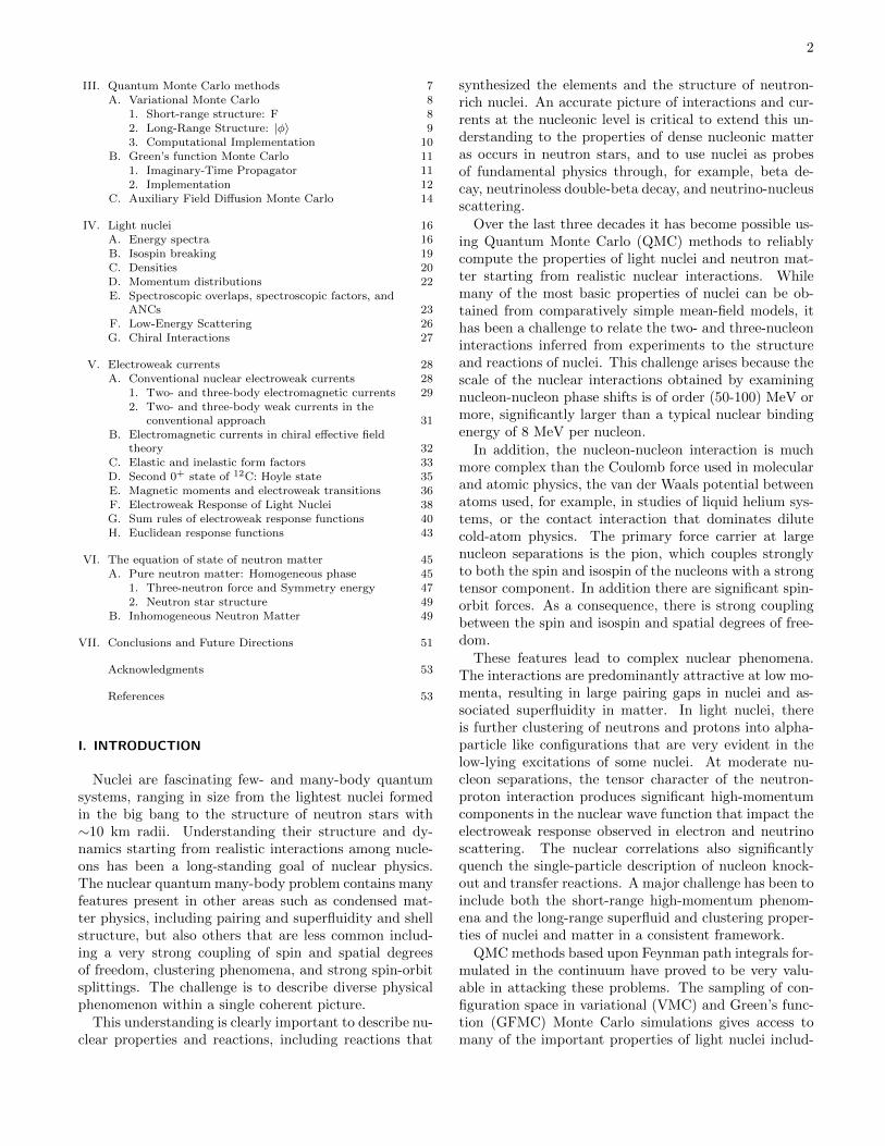
where the sum over i indicates the sum over samples ofthe wave function. The brackets in the numerator anddenominator of the last expression indicate sums overspins and isospins for each sample. The E(τ) initiallydecrease rapidly from the VMC (τ = 0) energy but thenstabilizes and just fluctuates within the statistical errors;examples of this are shown in Fig. 2, discussed below,and also in Sec. V.D. These stable values are averagedto get the converged GFMC results.
In principle, the GFMC propagation should con-verge to the lowest-energy state of given quantum num-bers Jπ;T . The nuclei considered here may have afew particle-stable and multiple particle-unstable excitedstates of the same quantum numbers. In practice, GFMCpropagation can obtain good energy estimates for manyof these additional states.
First, a set of orthogonal VMC trial functions are gen-erated that are diagonalized in the small single-particlep-shell basis of differing LS and spatial symmetry combi-nations that can make a given Jπ;T . These are pseudo-bound wave functions that fall off exponentially at longrange, with matter radii not much larger than the groundstate. Then independent GFMC propagations are carriedout starting from each of these trial functions. An exam-
ple is shown in Fig. 2 for the four 52
−p-shell states in 7Li,
all of which are particle-unstable (Pieper et al., 2004).The GFMC propagations stay nearly orthogonal to fairlylarge τ ∼ 1 MeV−1, as shown by the solid symbols in thefigure. The overlaps between different states can be eval-uated, and an explicit reorthogonalization made, shownby the open symbols. The states remain well-separatedin energy.
The first 52
−state in Fig. 2 is physically wide (∼ 900
keV) because it has the spatial symmetry of alpha plustriton and is several MeV above the threshold for breakupinto separated clusters. Consequently, a GFMC propaga-tion is expected to eventually drop to that threshold en-ergy, and the figure shows, after a rapid initial drop from−26 to −32 MeV by τ = 0.1 MeV−1, a slowly decreas-ing energy as τ increases, reaching −33 MeV at τ = 1MeV−1. In cases like this, the energy is quoted at thesmall value of τ where the rapid initial improvement overthe variational starting point has saturated. The second52
−state in Fig. 2 is physically narrow (∼ 80 keV) be-
cause it has a spatial symmetry like 6Li+n and is only20 keV above that breakup threshold. The GFMC prop-agation shows the same rapid initial drop in energy, andthen no appreciable further decline, allowing us to iden-
0 0.2 0.4 0.6 0.8 1-35
-30
-25
-20
-15
τ (MeV-1)
E(τ
) (
MeV
)
4th 5/2-
3rd 5/2-
2nd 5/2-
1st 5/2-
7Li(5/2-)AV18 + Illinois-2
GFMC Propagation
FIG. 2 GFMC energies of four 52
−states in 7Li vs. imaginary
time τ . The solid symbols show the computed energies at eachτ , open symbols show the results of rediagonalization.
tify a clear energy for this state. The third and fourth52
−states are not experimentally identified, but from the
GFMC propagation behavior we would expect the thirdstate to be physically narrow, and the fourth to be fairlybroad. An alternative approach to calculate systems inthe continuum by imposing specific boundary conditionsis presented in sec. IV.F.
In general the GFMC method suffers from the fermionsign problem, in that the numerator and denominatorof Eq. (45) tend to have an increasing ratio of error tosignal for a finite sample size and large imaginary timesτ . Other than for a few special cases such as purely at-tractive interactions, Hubbard models at half-filling, orlattice QCD at zero chemical potential, QMC methodstypically all have this difficulty. This is basically becausewhen ΨT is not exact it contains contamination fromthe Bosonic ground-state that will be unavoidably sam-pled. For scalar potentials, or in any case where a realwave function can be used, the sign problem is avoidedby using the fixed-node approximation, and the prob-lem is solved in a restricted (Bosonic) sub-space, wherethe trial wave function always maintains the same sign.In this case the problem would be exactly solved if thenodes of the true ground-state were known. Because thisis not the case, the solution obtained is a rigorous up-perbound to the true ground-state energy (Moskowitzet al., 1982). For spin-isospin dependent Hamiltoniansa complex wave function must be used, and the gen-eral fixed-node approximation does not apply. Insteadthe sign problem is circumvented by using a ‘constrainedpath’ algorithm, essentially limiting the original propa-gation to regions where the propagated and trial wavefunctions have a positive overlap. This approximation,
14
like the fixed-node algorithm for spin-independent inter-action, involves discarding configurations that have zerooverlap with the trial wave function. As such, they areexact for the case when the trial wave function is exactand are therefore variational. However, unlike the fixed-node case, the constrained path method does not provideupper bounds (Wiringa et al., 2000).
To address the possible bias introduced by the con-straint, all the configurations (including those that wouldbe discarded) for a previous number of steps Nuc are usedwhen evaluating energies and other expectation values.Nuc is chosen to be as large a number of time steps asfeasible with reasonable statistical error (again typically20 to 40 steps). Tests using different trial functions andvery long runs indicate that energies in p-shell nuclei areaccurate to around one per cent using these methods.This has been tested in detail in Wiringa et al. (2000),where the use of different wave functions is discussed.
Expectation values other than the energy are typicallycalculated from “mixed” estimates; for diagonal matrixelements this is:
〈O(τ)〉 ≈ 2〈ΨT |O|Ψ(τ)〉〈ΨT |Ψ(τ)〉
− 〈ΨT |O|ΨT 〉〈ΨT |ΨT 〉
. (46)
The above equation can be verified by assuming thatthe true ground state is well represented by the vari-ational wave function and a small perturbation, i.e.,|Ψ(τ)〉 ≈ |ΨT 〉+ λ|Ψ〉, and λ is a small parameter. Sincethe variational wave functions are typically very good theextrapolation is quite small. This can be further testedby using different trial wave functions to extract the sameobservable, or using the Hellman-Feynman theorem. Forthe case of simple static operators, improved methods areavailable that propagate both before and after the inser-tion of the operator O (Liu et al., 1974), i.e. directlycalculating operators with Ψ(τ) on both sides. Howeverthese techniques might be very difficult to apply for non-local operators.
Because a Hamiltonian commutes with itself, the totalenergy of the Hamiltonian used to construct the propa-gator [Eq. (42)] is not extrapolated; thus this total en-ergy is not the sum of its extrapolated pieces, rather thesum differs by the amount the ΨT energy was improved.As was noted above, the full AV18 NN potential can-not be used in the propagator; rather an H ′ containingthe AV8′ approximation to AV18 is used. In practiceAV8′ gives slightly more binding than AV18 so the therepulsive part of the 3N potential is increased to make〈H ′〉 ≈ 〈H〉. The difference 〈H − H ′〉 must be extrap-olated by Eq. (46). The best check of the systematicerror introduced by this procedure is given by comparingGFMC calculations of 3H and 4He energies with resultsof more accurate few-nucleon methods; this suggests thatthe error is less than 0.5% (Pudliner et al., 1997).
In the case of off-diagonal matrix elements, e.g., intransition matrix elements between initial Ψi and final
Ψf wave functions, Eq. (46) generalizes to:
〈O(τ)〉 ≈〈Ψf
T |O|Ψi(τ)〉〈Ψi
T |Ψi(τ)〉|ΨiT |
|ΨfT |
+〈Ψf (τ)|O|Ψi
T 〉〈Ψf (τ)|Ψf
T 〉|ΨfT |
|ΨiT |
−〈Ψf
T |O|ΨiT 〉
|ΨfT ||Ψi
T |. (47)
Technical details can be found in Pervin et al. (2007).Recently, the capability to make correlated GFMC
propagations has been added (Lovato et al., 2015). Inthese calculations, the values of R for every δτ time step,the corresponding weights W , and other quantities aresaved during an initial propagation. Subsequent propa-gations for different initial ΨT or different nuclei (suchas isobaric analogs) then follow the original propagationand correlated differences of expectation values can becomputed with much smaller statistical errors than forthe individual values.
C. Auxiliary Field Diffusion Monte Carlo
The GFMC method works very well for calculating thelow lying states of nuclei up to 12C. Its major limitationis that the computational costs scale exponentially withthe number of particles, because of the full summationsof the spin-isospin states. An alternative approach is touse a basis given by the outer product of nucleon posi-tion states, and the outer product of single nucleon spin-isospin spinor states. An element of this overcompletebasis is given by specifying the 3A Cartesian coordinatesfor the A nucleons, and specifying four complex ampli-tudes for each nucleon to be in a |s〉 = |p ↑, p ↓, n ↑, n ↓〉spin-isospin state. A basis state is then defined
|RS〉 = |r1s1〉 ⊗ |r2s2〉 · · · ⊗ |rnsn〉 . (48)
The trial functions must be antisymmetric under inter-change. The only such functions with polynomial scalingare Slater determinants or Pfaffians (BCS pairing func-tions), for example,
〈RS|Φ〉 = A [〈r1s1|φ1〉〈r2s2|φ2〉 . . . 〈rAsA|φn〉] (49)
or linear combinations of them. Operating on these withthe product of correlation operators, Eq. (23), again givesa state with exponential scaling with nucleon number. Inmost of the AFDMC calculations, these wave functionsinclude a state-independent, or central, Jastrow correla-tion:
〈RS|ΨT 〉 = 〈RS|
∏i<j
f c(rij)
Φ〉 . (50)
Calculations of the Slater determinants or Pfaffians scalelike A3 when using standard dense matrix methods, while
15
the central Jastrow requires A2 operations if its range isthe same order as the system size. These trial functionscapture only the physics of the gross shell structure ofthe nuclear problem and the state-independent part ofthe two-body interaction. Devising trial functions thatare both computationally efficient to calculate and thatcapture the state-dependent two- and three-body corre-lations that are important would greatly improve boththe statistical and systematic errors of QMC methodsfor nuclear problems.
The trial wave functions above can be used for varia-tional calculations. However, the results are poor sincethe functions miss the physics of the important tensorinteractions. More recently the improved form
〈RS|ΨT 〉 =
〈RS|
∏i<j
f c(rij)
1 +∑i<j
Fij +∑i<j<k
Fijk
|Φ〉 ,(51)
has been employed, where f c are spin-isospin indepen-dent correlations, and the correlations F have a formsimilar to those discussed in the previous sections. Thesewave functions can be used as importance functions forAFDMC calculations where they have been found ade-quate for this purpose in a variety of problems.
Using the basis state as in Eq. (48) requires the use ofa different propagator, with at most linear spin-isospinoperators. The propagator can be rewritten using theHubbard-Stratonovich transformation:
e−O2/2 =
1√2π
∫ ∞−∞
dx e−x2/2exO , (52)
where the variables x are called auxiliary fields, and Ocan be any type of operator included in the propagator.
It is helpful to apply the auxiliary field formalism toderive the well known central potential diffusion MonteCarlo algorithm (Anderson, 1976). The Hamiltonian is
H =
A∑n
p2n
2m+ V (R) , V (R) =
∑i<j
v(rij) , (53)
and v(rij) is a generic potential whose form depends onthe system. Making the short-time approximation, thepropagator can be written as
e−(H−E0)δτ ≈ exp
(−
A∑n
p2n
2mδτ
)exp [−(V (R)− E0)δτ ] .
(54)Since the Hamiltonian does not operate on the spin, thespin variables can be dropped from the walker expressionsto leave just a position basis |R〉. Operating with thelocal-potential term gives just a weight factor:
e−[V (R)−E0]δτ |R〉 = W |R〉 . (55)
The kinetic energy part of the propagator can be appliedby using the Hubbard-Stratonovich transformation:
exp
(−∑n
p2n
2mδτ
)≈∏n
exp
(− p
2n
2mδτ
)(56)
=∏n
1
(2π)3/2
∫dxne
−x2n/2 exp
(− i~pnxn
√~2δτ
m
).
This propagator applied to a walker |R〉 generates a newposition |R+∆R〉, where each particle position is shiftedas
r′n = rn +~2δτ
mxn . (57)
This is identical to the standard diffusion Monte Carloalgorithm without importance sampling. Each particle ismoved with a Gaussian distribution of variance ~2δτ/m,and a weight of exp[−(V (R) − E0)δτ ] is included. Thebranching on the weight is then included to complete thealgorithm.
The NN potential in the general form of Eq. (4) canbe written as
V =∑i<j
vp(rij)Opij =
1
2
∑i,j
Oαi Aiα,jβOβj =
1
2
∑n
λnO2n
(58)where Oαi are σi, τ i or similar combinations; see Gandolfi(2007) for more details. The new operators O are defined
On =∑jβ
ψ(n)jβ O
βj . (59)
Here ψ(n)jβ and λn are the eigenvectors and eigenvalues
obtained by diagonalizing the matrix Aiα,jβ .It is easy to see that applying the Hubbard-
Stratonovich transformation consists in a rotation of thespin-isospin states of nucleons:∏i<j
e−Vijδτ |RS〉 = (60)
∏n
1
(2π)3/2
∫dxne
−x2n/2 e
√−λnδτxnOn |RS〉 = |RS′〉 ,
The propagation is performed by sampling the auxiliaryfields from the probability distribution exp(−x2
n/2), andapplying the rotations to the nucleon spinors. At orderδτ the above propagator is the same as that described inthe previous sections. The advantage of this procedure isthat a wave function with the general spin-isospin struc-ture of Eq. (49) can be used, at a much cheaper compu-tational cost than that of including all the spin-isospinstates of Eq. (31). However, one must then solve the inte-gral in Eq. (52), which is done by Monte Carlo samplingof the auxiliary fields x.
The inclusion of importance sampling within the auxil-iary fields formalism is straightforward, and is currently
16
done as described in Sec. III.B.2. At each time-step arandom vector ∆R for the spatial coordinates, and therequired auxiliary fields X are sampled. The four weightscorresponding to these samples are
Wi =〈ΨI |R±∆RS′(±X)〉
〈ΨI |RS)〉exp [−Vc(R)δτ ] , (61)
where ΨI is used for the importance sampling, S′(X) areobtained by rotating the spinors S of the previous time-step using the auxiliary fields X, and Vc includes all thespin-isospin independent terms of the interaction. Theprocedure is then completed as done in GFMC: one ofthe above configurations is taken according to the proba-bilities, and the branching is done by considering the cu-mulative weight. This procedure lowers the variance asthe ”plus-minus” sampling cancels the linear terms com-ing from the exponential of Eqs. (56,60). Note that in theexample of the kinetic energy presented above, the effectof sampling using ±∆R is identical to sampling config-urations using ∇ΨI/ΨI commonly adopted in standarddiffusion Monte Carlo (Foulkes et al., 2001).
The importance function ΨI must be real and positive,and an efficient algorithm to deal with complex wavefunctions has been proposed by Zhang and Krakauer(2003), i.e., consider 〈ΨI |RS〉 = |〈ΨT |RS〉|, and mul-tiply the weight terms Wi by cos ∆θ, where ∆θ is thephase of 〈ΨT |R′ S′〉/〈ΨT |RS〉, and for each Wi, |R′ S′〉is the corresponding configuration obtained from the cor-responding ±∆R and ±X sampling. This method sam-ples configurations with a very low variance.
Previous applications of the AFDMC method used asomewhat different importance sampling, using ∇ΨI/ΨI
for the kinetic energy, and the strategy describedby Sarsa et al. (2003) and Gandolfi et al. (2009b) forthe spin; the two methods become the same in the limitof δτ → 0. In Gandolfi et al. (2014) it has been foundthat the procedure described above is much less time-step dependent for calculations including protons. Thisis due to the strong tensor force in the np channel thatin the case of pure neutron systems is very weak. Thetwo algorithms give very similar results.
The energy and other observables are calculated aftera block of steps in imaginary time, where each block com-prises a number of steps that is chosen to be large enough(typically around 100-500) such that the configurationsare statistically uncorrelated. This is done to save com-puting time in calculating observables for data that arenot useful to reduce the statistical errors.
While the Hubbard-Stratonovich transformation is themost common, there are many other possibilities. Forexample, the propagator for the relativistic kinetic energycan be sampled by using
exp[−(√
p2c2 +m2c4 −mc2)δτ]
=
∫d3xf(x)e−ip·x/~
(62)
with
f(x) =
∫d3p
(2π)3eip·x/~ e
−(√
p2c2+m2c4−mc2)δτ
= emc2δτ K2
(mc~√x2 + c2δτ2
)(63)
where K2 is the modified Bessel function of order 2 (Carl-son et al., 1993).
IV. LIGHT NUCLEI
A. Energy spectra
Results of GFMC calculations for light nuclei using theAV18+IL7 Hamiltonian are compared to experiment inFig. 3 and Table I (Brida et al., 2011; Lovato et al., 2013;McCutchan et al., 2012; Pastore et al., 2013, 2014; Pieperand Carlson, 2015; Wiringa et al., 2013). Results usingjust AV18 with no 3N potential are also shown in thefigure. Figure 3 shows the absolute energies of more than50 ground and excited states. The experimental energiesof the 21 ground states shown in the table are reproducedwith an rms error of 0.36 MeV and an average signederror of only 0.06 MeV. The importance of the three-body interaction is confirmed by the large correspondingnumbers for AV18 with no 3N potential, namely 10.0 and8.8 MeV. About sixty additional isobaric analog statesalso have been evaluated but are not shown here.
Table I gives the ground state energies E, proton (neu-tron) point radii rp (rn), magnetic moments µ (includ-ing two-body current contributions, see Sec. V), andquadrupole moments Q for all the particle-stable groundstates of A ≤ 10 nuclei, plus 12C and the resonant groundstates of 7He and 8Be. Many of these results were ob-tained in recent studies of spectroscopic overlaps, electro-magnetic transitions and sum rules, and isospin mixing.The energies, radii, and electromagnetic moments are ingenerally good agreement with experiment.
A detailed breakdown of the AV18+IL7 energies intovarious pieces for some of the nuclear ground states isshown in Table II. The components include the totalkinetic energy K, the contribution v18 of the strong in-teraction part of AV18, the full electromagnetic potentialvγij , the two-pion-exchange parts of IL7 V 2π
ijk , the three-
pion-ring parts V 3πijk , and the short-range repulsion V Rijk.
In the last column, δvij is the expectation value of thedifference between v18 and v8′ , which is the part of theNN interaction that is treated perturbatively because v8′
is used in the propagation Hamiltonian. The sum of thesix contributions K through V Rijk does not quite matchthe total energy reported in Table I because they havebeen individually extrapolated from the mixed energyexpression Eq. (46).
Several key observations can be drawn from Table II.First, there is a huge cancellation between kinetic and
17
-100
-90
-80
-70
-60
-50
-40
-30
-20E
nerg
y (M
eV)
AV18AV18+IL7 Expt.
0+
4He0+2+
6He 1+3+2+1+
6Li3/2−1/2−7/2−5/2−5/2−7/2−
7Li
0+2+
8He0+
2+2+
2+1+3+
1+
4+
8Li
1+
0+2+
4+2+1+3+4+
0+
8Be
3/2−1/2−5/2−
9Li
3/2−1/2+5/2−1/2−5/2+3/2+
7/2−
3/2−
7/2−5/2+7/2+
9Be
1+
0+2+2+0+3,2+
10Be 3+1+
2+
4+
1+
3+2+
3+
10B
3+
1+
2+
4+
1+
3+2+
0+
2+0+
12C
Argonne v18with Illinois-7
GFMC Calculations
FIG. 3 GFMC energies of light nuclear ground and excited states for the AV18 and AV18+IL7 Hamiltonians compared toexperiment. See Table I for references.
TABLE I AV18+IL7 GFMC results for A ≤ 12 nuclear ground states (Brida et al., 2011; Lovato et al., 2013; McCutchan et al.,2012; Pastore et al., 2013, 2014; Pieper and Carlson, 2015; Wiringa et al., 2013), compared to experimental values (Amrounet al., 1994; NNDC, 2014; Nortershauser and et al., 2009; Nortershauser et al., 2011; Purcell et al., 2010; Shiner et al., 1994;Tilley et al., 2002, 2004). Numbers in parentheses are statistical errors for the GFMC calculations or experimental errors;errors of less than one in the last decimal place are not shown.
AZ(Jπ;T ) E (MeV) rp [rn] (fm) µ (µN ) Q (fm2)GFMC Expt. GFMC Expt. GFMC Expt. GFMC Expt.
FIG. 4 GFMC excitation energies of light nuclei for the AV18 and AV18+IL7 Hamiltonians compared to experiment. SeeTable I for references.
two-body terms. Second, the net perturbative correctionδvij is tiny (< 2%) compared to the full v18 expectationvalue. Third, the total Vijk contribution is ∼ 5% of vij ,suggesting good convergence in many-body forces, but itis not negligible compared to the binding energy. Finally,the V 3π
ijk contribution that is unique to the Illinois poten-
tials is a small fraction of the V 2πijk in T = 0 states, but
does get as large as 35% in T = 2 states.
In describing the structure of the light nuclei, it is con-venient to characterize specific Jπ;T states by their dom-inant orbital and spin angular momentum and spatialsymmetry 2S+1LJ [n] where [n] denotes the Young dia-gram for spatial symmetry (Wiringa, 2006). (This classi-fication is essentially a modern update of the discussionin Feenberg and Wigner (1937).) For example, 4He isa 1S0[4] state, and the ground state of 6Li is predomi-nantly 3S1[42], with admixtures of 3D1[42] and 1P1[411].Because NN forces are strongly attractive in relative S-waves, and repulsive in P -waves, ground states of givenJπ;T have the maximum spatial symmetry allowed bythe Pauli exclusion principle. For the same spatial sym-metry, states of higher L are higher in the spectrum.Further, due to the effect of NN spin-orbit forces, iter-ated tensor forces and also 3N forces, the spin doublets,triplets, etc., are split, with the maximum J value forgiven [n] lying lowest in the spectrum (up to mid p-shell).These features are evident in the excitation spectra dis-
TABLE II Breakdown of GFMC energy contributions forAV18+IL7, in MeV. See Table I for references.
AZ(Jπ;T ) K v18 vγij V 2πijk V 3π
ijk V Rijk δvij2H(1+; 0) 19.81 −22.05 0.02 0.093H( 1
The excitations relative to the ground state energiesfor many states are shown in Fig. 4 and tabulated inTable III. These excitation energies are each the differ-ence of two independent GFMC calculations; the quotedstatistical errors are the uncorrelated combination of theerrors of each calculation. In general, the excitation en-
19
ergies are quite satisfactory with an rms error of 0.5 MeVfor 58 A ≤ 10 states using AV18+IL7 compared to 1.8MeV using just AV18. Thus we see that AV18 alone doesa much better job on excitation energies than it does forabsolute binding, and that the addition of IL7 greatlyimproves both aspects.
The 6He ground state is a 1S0[42] combination, with a1D2[42] first excited state; the AV18+IL7 Hamiltoniangets an excitation in fair agreement with experiment.The first three T = 0 excited states in 6Li constitutea 3DJ [42] triplet, and the spin-orbit splitting betweenthe 3+, 2+, and 1+ states is also reproduced very nicely.The first two states in 7Li are a narrowly split 2PJ [43]pair, while the next two are a 2FJ [43] pair, followedby the lowest member of a 4PJ [421] triplet, all with areasonably good reproduction of experiment. The 8Benucleus exhibits a strong 2α rotational spectrum, witha 1S0[44] ground state and widely spaced 1D2[44] and1G4[44] excited states, also with excitation energies inexcellent agreement with experiment. Above this rota-tional band are 3P2[431], 3P1[431], and 3D3[431] T = 0states that isospin mix with the T = 1 isobaric analogsof the 8Li ground and first two excited states.
The A = 10 nuclei, which are mid p-shell nuclei, havethe interesting feature of having two linearly independentways of constructing 2S+1DJ [442] states. In 10Be, theground state is 1S0[442] (much like 6He with an addedα) followed by two 1D2[442] excited states. In 10B, thelowest state might be expected to be a 3S1[442] statesimilar to 6Li ground state plus an α, but there are alsotwo 3DJ [442] triplets, one of which is so widely split bythe effective one-body spin-orbit force that one 3D3[442]component becomes the ground state leaving the 3S1[442]state as the first excited state (Kurath, 1979).
The IL7 3N force plays a key role in getting thesespin-orbit splittings correctly. The AV18 NN force alonesplits the 6Li 3DJ [42] states in the correct order, butwith insufficient spacing. It leaves the 7Li 2PJ [43] dou-blet degenerate, as well as the two 1D2[442] states in10Be, and the 3S1[442] state in 10B is predicted to bethe ground state. IL7 not only splits the two 2+ statesin 10Be by about the correct amount, but splits themin the correct direction, making the predicted E2 transi-tions to the ground state significantly different in size asexperimentally observed (McCutchan et al., 2012). Byincreasing the splitting of the 3DJ [442] states in 10B, IL7also gives the correct 3+ ground state for 10Be. Addi-tion of the older Urbana 3N potentials fixes some, butnot all of these problems. The superior behavior of theIllinois 3N interactions is also seen in 5He, i.e., αn scat-tering, as discussed in Sect. IV.F. The importance of3N interactions is also observed in no-core shell modelcalculations (Navratil et al., 2007).
TABLE III GFMC excitation energies in MeV for theAV18+IL7 Hamiltonian compared to experiment (Tilleyet al., 2004) for selected A ≤ 12 states; those marked witha * are the empirical isospin-unmixed values. See Table I forreferences.
Energy differences among isobaric analog states areprobes of the charge-independence-breaking parts of theHamiltonian. The energies for a given isospin multipletcan be expanded as
nomials (Peshkin, 1960). GFMC calculations of the co-efficients an(A, T ) for a number of isobaric sequences andvarious contributions for the AV18+IL7 Hamiltonian areshown in Table IV along with the experimental values.The contributions are the CSB component of the kineticenergyKCSB, all electromagnetic interactions vγ , and thestrong CIB interactions, vCIB = vCSB +vCD. The experi-mental values were computed using ground-state energiesfrom (NNDC, 2014) and excitation energies from (TUNL,2014). By using the correlated GFMC propagations de-scribed in Sec. III.B, it is possible to extract statisticallysignificant values for some of the a3(A, T ). An additionalcontribution is the second-order perturbation correction
20
TABLE IV GFMC isovector and isotensor energy coefficientsan(A, T ) computed using AV18+IL7, in keV, compared toexperiment (Pieper, 2015; Wiringa et al., 2013).
to the CI part of the Hamiltonian δHCI due to differ-ences in the wave functions. Although this term is small,it is the difference between two large energies and has thegreatest Monte Carlo statistical error of any of the con-tributions; again correlated GFMC propagations makeits extraction possible.
The dominant piece in all these terms is the Coulombinteraction between protons, giving 85-95% (70-100%) ofthe experimental isovector (isotensor) total. However thestrong CSB and CD interactions give important correc-tions, and the other terms are not negligible. In particu-lar, the vCSB contribution is just the right size to fix the3He – 3H mass difference and is a strong constraint on thedifference of nn and pp scattering lengths. Overall, theisoscalar terms are in good agreement with experiment,while the isotensor terms are perhaps a little too large.One can understand the negative values of a3(A, T ) ascoming from the increasing Coulomb repulsion as Tz in-creases; this expands the nucleus and reduces vC1(pp).
Another place that CSB interactions play a role is inthe isospin mixing of nearby states with the same spinand parity but different isospins (Wiringa et al., 2013).A classic case is the appearance in the 8Be excitationspectrum of three pairs of states with Jπ of 2+ (at 16.6–16.9 MeV), 1+ (at 17.6–18.2 MeV) and 3+ (at 19.0–19.2MeV). The unmixed states come from three T = 0 states,including the second 2+ excitation and first 1+ and 3+
states in the 8Be spectrum and three T = 1 states thatare the isobaric analogs of 8Li ground state and its firsttwo excited states. These states have the same dominant[431] spatial symmetry, so it is not surprising that theirenergies are closely paired. The CSB components of theHamiltonian have ∼ 100 keV off-diagonal (in isospin) ma-
TABLE V GFMC isospin mixing matrix elements H01 in8Be spin doublets computed using AV18+IL7 (augmentedby class IV CSB contributions) in keV, compared to experi-ment (Wiringa et al., 2013).
trix elements H01 leading to significant isospin mixing..Experimentally this is observed in the two-alpha decay ofthe 2+ states, which have comparable widths and whichcan only go via the T = 0 component of the wave func-tions. The mixing of the 1+ doublet is apparent in theirM1 decays (Pastore et al., 2014).
GFMC calculations of the isospin-mixing matrix ele-ments are shown in Table V. The table includes a smallcontribution from class IV CSB terms vIV that can con-nect T = 0 and T = 1 np pairs (Henley et al., 1979).The theoretical total provides about 90% of the inferredexperimental values in the 2+ and 1+ doublets, but is toolarge for the (poorly determined) 3+ case.
C. Densities
The one- and two-nucleon density distributions of lightnuclei are interesting in a variety of experimental set-tings. They are evaluated as the expectation values
ρN (r) =1
4πr2〈Ψ|
∑i
PNiδ(r − |ri −Rcm|)|Ψ〉 , (65)
ρNN (r) =1
4πr2〈Ψ|
∑i<j
PNiPNj
δ(r − |ri − rj |)|Ψ〉 , (66)
where PN is a proton or neutron projector.Ground state proton and neutron rms point radii are
tabulated in Table I. These can be related to the chargeradii, which have been measured very accurately for thehelium, lithium, and beryllium isotopic chains in recentyears by a combination of electron scattering from sta-ble nuclei and isotopic differences by atomic spectroscopyon rare isotopes. A recent review (Lu et al., 2013) dis-cusses these developments and the conversion betweenpoint and charge radii and presents figures for the GFMCone- and two-body densities of the helium isotopes.
The proton and neutron one-body densities for thelithium isotope chain are shown, as red up triangles andblue down triangles, respectively, in the upper panels ofFig. 5. As the binding energy increases with A, the cen-tral proton density increases, even though the number ofprotons is constant. Consequently, the proton point ra-dius decreases by 0.4 fm in going from 6Li to 9Li, in fairagreement with the experimentally observed reduction of
21
0 1 2 3 40.00
0.02
0.04
0.06
0.08
0.10
0.12
9Li(3/2-)
0 1 2 3 40.00
0.02
0.04
0.06
0.08
0.10
0.12
8Li(2+)
0 1 2 3 40.00
0.02
0.04
0.06
0.08
0.10
0.12
7Li(3/2-)
0 1 2 3 40.00
0.02
0.04
0.06
0.08
0.10
0.12
ρ(r)
(fm
-3)
6Li(1+)
0 1 2 3 4-0.04
-0.02
0.00
0.02
0.04
r (fm)
0 1 2 3-0.04
-0.02
0.00
0.02
0.04
r (fm)
0 1 2 3-0.04
-0.02
0.00
0.02
0.04
r (fm)
0 1 2 3-0.04
-0.02
0.00
0.02
r (fm)
ρ µ(r
) (µ
N f
m-3
)
FIG. 5 GFMC point proton (red up triangles) and neutron (blue down triangles) densities (upper panel) and magnetic spindensities (lower panel) for the chain of lithium isotopes; also shown are proton magnetic orbital density (green diamonds), andtotal magnetic density in IA (black circles) (Wiringa, 2015).
0.34 fm. In contrast, the neutron point radius is relativelyconstant, even though neutrons are being added, varyingonly 0.15 fm over the same range.
The magnetic moments of A ≤ 9 nuclei have been cal-culated in GFMC (Marcucci et al., 2008; Pastore et al.,2013; Pervin et al., 2007) including contributions fromtwo-body meson-exchange currents (MEC), as discussedin Sec. V. The MEC can give 20–40% contributions overthe impulse approximation (IA) values, resulting in verygood agreement with experiment as shown in Table I.
The origin of the IA contributions from the protonand neutron spin densities and proton orbital densityare illustrated in the bottom panels of Fig. 5, also forthe lithium isotope chain. Here, the proton spin con-tribution µp[ρp↑(r)− ρp↓(r)] is shown by red upward-pointing triangles, the neutron spin contribution by bluedownward-pointing triangles, the proton orbital contri-bution by green diamonds, and the total by black cir-cles. The proton spin density, due to one unpaired p-shell proton, is similar in all cases, with a negative regionat short distance from the core and a positive peak near2 fm that gradually shifts inward as the binding increases.The neutron spin density has the opposite sign and al-ternates between a significant unpaired neutron contri-bution in 6,8Li and a very small paired contribution in7,9Li. The proton orbital piece gets progressively largeras A increases. The MEC contributions are discussed inmore detail below, but come largely from pion exchangeand are primarily isovector in character, ranging from 2%in 6Li to 10% in 7Li and 20% in 8,9Li.
0 1 2 3 4 50.000
0.004
0.008
0.012
0.016
0.020
0.024
0.028
0.032
r (fm)
ρ pp(r
) (f
m-3
)
9Li8Li7Li6Li
FIG. 6 GFMC pp densities for the chain of lithium iso-topes (Wiringa, 2015).
The two-nucleon density for pp pairs in the lithiumisotopes is shown in Fig. 6 and all four curves integrateto three pairs. Because the third proton is in the p-shell, the behavior of ρpp(r) is rather different from theone pp pair in the core of the helium isotopes shown inFig. 12 of Lu et al. (2013). In that case, there is a slightdecrease in the peak value as A increases because the p-shell neutrons in 6,8He tug the core protons out a little. Inlithium the peak value of ρpp(r) gets progressively largerwith increasing A due to the increasing binding, so thepair rms radius decreases from 4.03 fm in 6Li to 3.20 fm
22
0 1 2 3 4 510-3
10-1
101
103
12C
0 1 2 3 4 510-3
10-1
101
103
10B
0 1 2 3 4 510-3
10-1
101
103
8Be
0 1 2 3 4 510-3
10-1
101
103
6Li
0 1 2 3 4 510-3
10-1
101
103
4He
0 1 2 3 4 510-3
10-1
101
103
k (fm-1)
ρ p(k)
(fm
3 )
2H
FIG. 7 VMC proton momentum distributions in T = 0 lightnuclei (Wiringa et al., 2014).
in 9Li.
D. Momentum distributions
Momentum distributions of individual nucleons, nu-cleon pairs, and nucleon clusters reflect features of theshort-range structure of nuclei. They can provide use-ful insight into various reactions on nuclei, such as(e, e′p) and (e, e′pp/pn) electrodisintegration processes orneutrino-nucleus interactions.
The probability of finding a nucleon with momentumk and spin-isospin projection σ,τ in a given nuclear stateis proportional to the density
ρστ (k)=
∫dr′1 dr1 dr2 · · · drA ψ†JMJ
(r′1, r2, . . . , rA)
× e−ik·(r1−r′1) Pστ (1)ψJMJ
(r1, r2, . . . , rA) . (67)
Pστ (i) is the spin-isospin projection operator for nucleoni, and ψJMJ
is the nuclear wave function with total spinJ and spin projection MJ . The normalization is
Nστ =
∫dk
(2π)3ρστ (k) , (68)
where Nστ is the number of spin-up or spin-down protonsor neutrons.
Early variational calculations of few-nucleon momen-tum distributions (Schiavilla et al., 1986) evaluatedEq. (67) by following a Metropolis Monte Carlo walk inthe dr1 dr2 · · · drA space and one extra Gaussian integra-tion over dr′1 at each Monte Carlo configuration. Thiswas subject to large statistical errors originating fromthe rapidly oscillating nature of the integrand for largevalues of k.
0 1 2 3 4 510-1
101
103
105
12C
0 1 2 3 4 510-1
101
103
105
10B
0 1 2 3 4 510-1
101
103
105
8Be
0 1 2 3 4 510-1
101
103
105
6Li
0 1 2 3 4 510-1
101
103
105
q (fm-1)
ρ pN(q
,Q=
0) (
fm3 )
4He
FIG. 8 VMC pn (blue diamonds) and pp (red circles) back-to-back (Q = 0) pair momentum distributions for T = 0nuclei (Wiringa et al., 2014).
and perform the Gaussian integration over x. How-ever, this requires re-evaluating both initial and finalwave functions at multiple configurations, which limitsthe present calculations to VMC. A comprehensive setof single-nucleon momentum distributions for A ≤ 12nuclei, evaluated with the AV18+UX Hamiltonian, hasbeen published (Wiringa et al., 2014) with figures andtables available on-line (Wiringa, 2014a).
The overall evolution of the proton momentum distri-bution in light T = 0 nuclei is shown in Fig. 7. The shapeof the distributions shows a smooth progression as nucle-ons are added. As A increases, the nuclei become moretightly bound, and the fraction of nucleons at zero mo-mentum decreases. As nucleons are added to the p-shell,the distribution at low momenta becomes broader, anddevelops a peak at finite k. The sharp change in slopenear k = 2 fm−1 to a broad shoulder is present in all thesenuclei and is attributable to the strong tensor correlationinduced by the pion-exchange part of the NN potential,further increased by the two-pion-exchange part of the3N potential. Above k = 4 fm−1, the bulk of the mo-mentum density appears to come from short-range spin-isospin correlations.
Two-nucleon momentum distributions, i.e., the proba-bility of finding two nucleons in a nucleus with relativemomentum q = (k1−k2)/2 and total center-of-mass mo-mentum Q = k1+k2, provide insight into the short-rangecorrelations induced by a given Hamiltonian. They can
23
0 1 2 3 4 510-2
100
102
104Q=0.00
4He
0 1 2 3 4 510-2
100
102
1040.25
0 1 2 3 4 510-2
100
102
1040.50
0 1 2 3 4 510-2
100
102
1040.75
0 1 2 3 4 510-2
100
102
1041.00
0 1 2 3 4 510-2
100
102
104
q (fm-1)
ρ pp(q
,Q)
(fm
3 )
1.25
FIG. 9 VMC proton-proton momentum distributions in 4Heaveraged over the directions of q and Q as a function of q forseveral fixed values of Q from 0 to 1.25 fm−1 (Wiringa et al.,2014).
be formulated analogously to Eqs. (67,69), and projectedwith total pair spin-isospin ST , or as pp, np, and nnpairs. Again, a large collection of VMC results has beenpublished (Wiringa et al., 2014) and figures and tablesare available on-line (Wiringa, 2014b).
Experiments to search for evidence of short-range cor-relations have been a recent focus of activity at Jeffer-son Laboratory. In an (e, e′pN) experiment on 12C atJLab, a very large ratio ∼ 20 of pn to pp pairs wasobserved at momenta q=1.5–2.5 fm−1 for back-to-back(Q = 0) pairs (Subedi et al., 2008). VMC calculationsfor ρpN (q,Q = 0) are shown in Fig. 8 as blue diamondsfor pn pairs and red circles for pp pairs for T = 0 nucleifrom 4He to 12C (Schiavilla et al., 2007; Wiringa et al.,2014). The pp back-to-back pairs are primarily in 1S0
states and have a node near 2 fm−1, while the pn pairsare in deuteron-like 3S1 −3 D1 states where the D-wavefills in the S-wave node. Consequently, there is a largeratio of pn to pp pairs in this region. This behavior ispredicted to be universal across a wide range of nuclei.
As Q increases, the S-wave node in pp pairs will gradu-ally fill in, as illustrated for 4He in Fig. 9, where ρpp(q,Q)is shown as a function of q for several fixed values of Q,averaged over all directions of q and Q. In contrast, thedeuteron-like distribution in pn pairs is maintained as Qincreases, as shown in Fig. 10, with only a gradual de-crease in magnitude because there are fewer pairs at hightotal Q. Recently, these momentum distributions for 4Hehave been tested in new JLab experiments and found topredict the ratio of pp to pn pairs at higher missing mo-mentum very well (Korover et al., 2014).
0 1 2 3 4 510-1
101
103
105Q=0.00
4He
0 1 2 3 4 510-1
101
103
1050.25
0 1 2 3 4 510-1
101
103
1050.50
0 1 2 3 4 510-1
101
103
1050.75
0 1 2 3 4 510-1
101
103
1051.00
0 1 2 3 4 510-1
101
103
105
q (fm-1)
ρ pn(q
,Q)
(fm
3 )
1.25
FIG. 10 VMC proton-neutron momentum distributions in4He averaged over the directions of q and Q as a function ofq for several fixed values of Q from 0 to 1.25 fm−1 (Wiringaet al., 2014).
E. Spectroscopic overlaps, spectroscopic factors, and ANCs
Determining the influence of nuclear structure on nu-clear reactions is a challenging subject. One source oftheoretical input is the calculation of spectroscopic over-laps, spectroscopic factors (SFs), and asymptotic normal-ization coefficients (ANCs). They are steps on the wayto calculating reaction cross sections in direct nuclear re-actions, like nucleon knockout or radiative capture.
A one-nucleon spectroscopic overlap is the expectationvalue of the nucleon removal operator between states ofnuclei differing by one particle. It can be written as
R(β, γ, ν; r) =√A⟨
[ΨA−1(γ)⊗ Y(ν; rCv)]JA,TA∣∣∣∣δ(r − rCv)r2Cv
∣∣∣∣ΨA(β)
⟩(70)
where β ≡ A, JπA, TA, Tz,A denotes the quantum num-bers of a parent A-body nucleus, γ ≡ C, JπC , TC , Tz,Cspecifies an (A − 1)-body core, and ν ≡ v, l, s, j, t, tzspecifies the valence nucleon. Here rCv is the distancebetween the valence nucleon and the center of mass ofthe core, and Y(ν; r) ≡ [Yl(r)⊗ χs(σv)]j χt,tz (τv) is thevalence angle-spin-isospin function. The SF is then de-fined as the norm of the overlap:
S(β, γ, ν) =
∫|R(β, γ, ν; r)|2 r2dr. (71)
In standard shell model calculations (Cohen and Ku-rath, 1967), the SFs obey various sum rules (Macfarlaneand French, 1960), including that for a given state ofthe parent nucleus, the SFs to all possible final statesof the core plus valence nucleon add up to the parent’snumber of such nucleons. For example,
∑γ,ν〈6He(γ) +
p(ν)|7Li(β)〉 = 1 because 7Li has one p-shell proton.
24
0 2 4 6 8r [fm]
10-3
10-2
10-1
R [
fm-3
/2]
VMCmixed
6He
mixed 7Li
GFMCfitW/r
FIG. 11 VMC and GFMC calculations of the 〈6He(0+) +
p(p3/2)|7Li( 32
−)〉 overlap (Brida et al., 2011); see text for de-
tails.
Overlap functions R(r) satisfy a one-body Schrodingerequation with appropriate source terms (Pinkston andSatchler, 1965). Asymptotically, at r →∞, these sourceterms contain core-valence Coulomb interaction at most,and hence the long-range part of overlap functions forparent states below core-valence separation thresholds isproportional to a Whittaker function W−η,l+1/2:
R(β, γ, ν; r)r→∞−−−→ C(β, γ, ν)
W−η,l+1/2(2kr)
r, (72)
where η = ZCZνα√µc2/2|B| depends on proton num-
bers ZC and Zν , the fine-structure constant α, and thecore-valence reduced mass µ and the separation energy B(negative for parent states below core-valence separationthresholds). The wave number k is defined as
√2µ|B|/~,
and l is the orbital momentum in Y(ν). The proportion-ality constant C(β, γ, ν) in Eq. (72) is the ANC.
VMC calculations of overlaps and SFs for s-shell nucleiwere first reported in (Schiavilla et al., 1986), followedby calculations in various p-shell nuclei for applicationto (e, e′p) experiments (Lapikas et al., 1999), transfer re-actions like (d, p) and (d,3 He) (Wuosmaa et al., 2005,2008), and single-neutron knockout reactions (Grinyeret al., 2011, 2012). The first GFMC calculations forA ≤ 7 nuclei were reported in Brida et al. (2011). Theseare off-diagonal calculations, as in Eq. (47), so the finalGFMC result is extrapolated from two different mixedestimates, one where Ψ(τ) is propagated for the A-bodynucleus and one where it is propagated for the (A − 1)-body nucleus. A large collection of VMC and GFMCresults can be found on-line (Wiringa and Brida, 2014).
For the s-shell nuclei, VMC energies and densities arevery close to the exact GFMC results, so VMC andGFMC overlaps R(r) for cases like 〈3H + p(s1/2)|4He〉are in excellent agreement, both in the peak values atsmall r and in the asymptotic regime. This translatesinto very similar SF and ANC predictions. However, for
0 2 4 6 8r [fm]
0
2
4
6
C(r
)
VMCGFMCfit
FIG. 12 The ratios C(r) of the VMC and GFMC 〈6He(0+) +
p(p3/2)|7Li( 32
−)〉 overlaps to the asymptotic Whittaker func-
tion (Brida et al., 2011); see text for details.
p-shell nuclei, the VMC energies are progressively smallerin magnitude relative to GFMC as A increases, althoughthe one-body densities remain fairly close. Consequentlythe overlaps have similar peak values but different asymp-totic behavior.
An example of p-shell overlap calculations is shown in
Fig. 11 for 〈6He(0+)+p(p3/2)|7Li( 32
−)〉. The VMC calcu-
lation is shown by black squares, the two GFMC mixedestimates by red down (blue up) triangles for GFMCpropagation of the 6He (7Li) states, and the final GFMCresult by green circles. In this case, the VMC overlap andthe GFMC mixed estimate when 6He is propagated givevirtually identical results, so the GFMC mixed estimatewhen 7Li is propagated coincides with the final result.The smooth fit to the GFMC result shown by the solidpurple line is parallel at large r to the Whittaker functionW/r (constructed with the experimental separation en-ergy) shown by the dot-dash orange line. The integratedVMC and GFMC SFs for this case are 0.44 and 0.41, re-spectively. These values are consistent with experiment(Lapikas et al., 1999; Wuosmaa et al., 2008) but muchsmaller than the standard shell model value (correctedfor center of mass) of 0.69 (Cohen and Kurath, 1967).
In general, the SFs predicted by the VMC and GFMCcalculations show a significant quenching relative to stan-dard shell model estimates which are based on notions ofindependent particle motion. The low-energy states oflight nuclei can be interpreted as having quasiparticlesin single-particle orbitals (Pandharipande et al., 1997).The difference between physical particles and quasiparti-cles is the consequence of the correlations in the system,which push a significant fraction of nucleons above thenominal Fermi sea, as noted in the momentum distribu-tion calculations of Sec. IV.D. The SF is the quasiholestrength, i.e., the probability of the quasiparticle beinga physical particle. A variety of experiments find that,for a broad range of nuclei from 4He to 208Pb, SFs are
25
FIG. 13 Overlaps for various bound states as computed by 1) VMC sampling (points with error bars), 2) a bound-state integralrelation with the VMC as input but imposing experimental separation energies (solid curves) evaluated by Nollett (2012), and3), GFMC overlaps (dashed curves) from Brida et al. (2011).
quenched ∼ 0.5 relative to standard shell model, consis-tent with the VMC and GFMC calculations (Kay et al.,2013).
The ratio C(r) of the VMC and GFMC overlaps withthe Whittaker function constructed with the experimen-tal separation energy are shown in Fig. 12. The incorrectasymptotic behavior of the VMC calculation means theC(r) does not reach a constant value and precludes ex-tracting a reasonable ANC from this ratio. However theGFMC calculation, with its much better asymptotic be-havior, does go to a constant at large r, as indicated bythe purple line fit.
There is an alternative method to obtain overlaps,ANCs, and estimates of widths from variational wavefunctions using integral constraints that are insensitiveto their asymptotic behavior (Barletta et al., 2009; Nol-lett, 2012; Nollett and Wiringa, 2011). As an example,the ANC is given by a sort of modified overlap integralwith a finite-range potential insertion:
C(β, γ, ν) =2µ
k~2w×A
∫ M−η,l+ 12(2kr)
r(73)
Ψ†A−1(γ)Y†(ν; r) (Urel − VC) ΨA(β) d3r .
The integral extends over all particle coordinates, A isan antisymmetrization operator for the core and valenceparticle, M−η,l+ 1
2is the Whittaker function that is irreg-
ular at infinity, and w is its Wronskian with the regularWhittaker function W−η,l+ 1
2. The Urel is a sum of two-
and three-body potentials involving the last nucleon
Urel =∑i<A
viA +∑
i<j<A
VijA , (74)
where we have labeled the last nucleon A. The point-Coulomb potential between the residual nucleus and lastnucleon is VC = ZA−1Zνα~c/r and in the limit of largeseparation, typically r > 7 fm, (Urel−VC) vanishes. Thisprovides a natural cutoff to the integral of Eq. (73).
This integral method has been implemented, usingVMC wave functions obtained for the AV18+UIX Hamil-tonian, for 19 one-nucleon removals from nuclear stateswith 3 ≤ A ≤ 9. Detailed tables are given in Nollett andWiringa (2011), as well as comparisons to available ex-perimental determinations and previous theoretical work.In general, when the experimental binding energyBexpt isused in the wave number k, the ANCs derived from VMCwave functions through Eq. (73) are in excellent agree-ment with experiment. The results also agree with theGFMC determinations discussed above at ∼ 10% level,
e.g., the GFMC ANC for 〈6He(0+) + p(p3/2)|7Li( 32
−)〉
from Fig. 12 is 3.5, while the VMC integral value is3.7. Of particular note, the astrophysical S-factor for8B → p +7 Be is related to the ANCs by S17(0) =
[38.7 eV b fm]∑
j |C(2+, 32
−, j)|2 (Esbensen, 2004). In-
serting the VMC ANC values gives the result 20.8 eV b,which is exactly the current recommended value from theSolar Fusion II analysis (Adelberger et al., 2011).
26
Relations similar to Eq. (73) can be used to gener-ate overlaps and also to estimate the widths of resonantstates (Nollett, 2012). Examples of overlaps evaluated inthis way are shown in Fig. 13, where they are comparedto the VMC input and the GFMC overlaps of Brida et al.(2011). Many widths in 5 ≤ A ≤ 9 nuclei have also beenevaluated, using as input VMC pseudo-bound wave func-tions from the AV18+UIX Hamiltonian. Detailed tablesare given in Nollett (2012). The agreement with experi-ment is generally satisfactory when the physical states arenarrow, but the method fails for broad states; the over-laps can help differentiate these cases. For broad states,true scattering wave functions need to be developed, asdiscussed below.
While the preceding discussion has focused on single-nucleon spectroscopic overlaps, SFs, ANCs, and widths,the techniques involved are readily adaptable to othercluster-cluster pairings, e.g., with deuterons or αs as thevalence cluster. Spectroscopic overlaps for dd in 4He, αdin 6Li, and αt in 7Li are included in the on-line overlaptabulations of Wiringa and Brida (2014) and spectro-scopic factors can be obtained from the cluster-clustermomentum distribution tables in Wiringa (2014a). Itshould be possible in future to evaluate α ANCs andwidths from the VMC wave functions and generalizedintegral relations.
F. Low-Energy Scattering
Quantum Monte Carlo methods can also be used totreat low-energy scattering in nuclear systems (Carlsonet al., 1987; Nollett et al., 2007). The methods employedare similar to bound-state methods, and are easily appli-cable at low energies where the combined system breaksup into at most two clusters. One enforces one or moreboundary conditions on the asymptotic wave function atlarge cluster separations and then solves for the energylevels with these boundary conditions. The resulting en-ergies can be used with the boundary conditions to de-termine the elements of the S-matrix for those energies.
The simplest example is for a one-channel case withonly elastic scattering, for example n−α scattering. Theasymptotic wave function for the relative motion of theneutron and the alpha particle is given by:
Ψ ∝ Φc1Φc2YLJ [cos δJLjL(kr)− sin δJLnL(kr)] ,(75)
where Φc1 and Φc2 are the internal wave functions of thetwo clusters, k and r are the relative momentum andspatial separation between the two clusters, and δJL isthe phase shift in the JL partial wave. For problems withCoulomb interactions between the clusters the relativewave function will contain Coulomb rather than Besselfunctions.
The original QMC scattering calculations required thewave function to be zero at a specified cluster separa-
tion (Carlson et al., 1987), while in recent work the log-arithmic derivative γ of the relative wave function at aboundary r = R0 is specified (Nollett et al., 2007):
γ =∇rΨ
Ψ
∣∣∣∣∣r=R0
. (76)
In VMC calculations this is enforced within the form ofthe trial wave function, which is required at large dis-tances to go like Eq. (75). The radius R0 should be largeenough so that there is no strong interaction betweenthe clusters at that separation. The scattering energyand hence the relative momentum between clusters is un-known initially, but these are obtained by variationallysolving for states confined within the boundary r = R0.Knowledge of the energy and the boundary condition isthen sufficient to determine the phase shift at that en-ergy. The method for GFMC is very similar, except thatthe logarithmic derivative of the wave function must alsobe enforced in the propagator. This can be incorporatedthrough an image method. For each point R near theboundary r = R0 reached during the random walk, thecontribution to the internal wave function from pointsoriginally outside the boundary are added. Consider animage at a cluster separation re = r(R0/r)
2; simple ma-nipulations yields
Ψn+1(R′) =
∫|r|<R0
dRc1 dRc2 dr G(R′,R) (77)
×[Ψn(R) + γ
G(R′,Re)
G(R′,R)
(rer
)3
Ψn(Re)
],
where R and R′ are the initial and final points of all theparticles, Rc1 and Rc2 are the internal coordinates of theclusters, and r is the separation between clusters. Theimage point for all the particles is denoted by Re, and reis its cluster separation. The image contribution ensuresthe correct logarithmic derivative of the wave function atthe boundary is preserved in the propagation.
The n−α system is interesting as it is the lightest sys-tem where T = 3/2 triplets play a significant role. QMCmethods have been used to study low-energy scattering inn−α, including the two low-lying P -wave resonances andS-wave scattering (Nollett et al., 2007). The spin-orbitsplitting is especially interesting, as it can be examinedby comparing the 3P1/2 and 3P3/2 partial waves.
The results of calculations with the AV18 NN inter-action and with different 3N interactions are shown inFig. 14. The various calculations are also compared withan R-matrix analysis of the experimental data. As is ev-ident from the figure, the AV18 interaction alone signif-icantly underpredicts the spin-orbit splitting. The two-pion-exchange in the UIX 3N interaction increases thesplitting, but not enough to agree with the experimentaldata. The IL2 model of the 3N interaction results in goodagreement with the experimental spin-orbit splitting.
27
0 1 2 3 4 50
30
60
90
120
150
180
Ec.m. (MeV)
δ JL (
degr
ees)
12
+
12
-
AV18AV18+UIXAV18+IL2R-Matrix
32
-
FIG. 14 (Color online) Phase shifts for n-α scattering. Filledsymbols (with statistical errors smaller than the symbols) areGFMC results, dashed curves are polynomial fits, and solidcurves are from an R-matrix fit to data (Nollett et al., 2007).
These scattering methods have many possible appli-cations. They can be extended to inelastic multichan-nel processes in a fairly straightforward manner. In thiscase there are multiple independent solutions for a givenscattering energy, hence one must study the energy asa function of the boundary conditions in each channeland obtain multiple independent solutions for the sameenergy. From the boundary conditions, the energy, andthe relative asymptotic magnitude of the wave functions,one can obtain the full multichannel S-matrix. It shouldbe possible to treat a variety of low-energy strong reac-tions, as well as electroweak transitions involving scat-tering states using these methods. In addition, hadronicparity violation in few-nucleon systems is an importantapplication.
G. Chiral Interactions
Local NN potentials derived within chiral effectivefield theory have been used to calculate properties ofA=3,4 nuclei with GFMC by Lynn et al. (2014). Al-though the calculations do not yet include 3N interac-tions that also appear at N2LO, they are neverthelessinteresting, showing the order-by-order results for thebinding energies and also the range of results for differentcutoffs. Also the question of perturbative treatments ofhigher-order corrections has been investigated, as well as
-48
-46
-44
-42
LO NLO N2LO NLO+pert. v8
′
Eb [
Me
V]
Chiral Order
-30
-28
-26
-24
-22
-20
-18
-16
Exp.R0 = 1.0 fmR0 = 1.1 fmR0 = 1.2 fm
FIG. 15 GFMC 4He binding energies at LO, NLO, and N2LOcompared with experiment (dashed line) and with the Ar-gonne AV8′ energy. Also shown is a first-order perturbation-theory calculation of the N2LO binding energy using the NLOwave function (Lynn et al., 2014).
one- and two-nucleon distributions.
Figure 15 shows results at various orders and for differ-ent values of the cutoff R0 used to regulate the small-rbehavior of the pion-exchange potentials, flong = 1 −exp[−(r/R0)4]. The LO result is extremely overbound,whereas the NLO and N2LO results are underbound asexpected because of the lack of the 3N interaction. TheNLO interaction includes pion-exchange diagrams, andthe N2LO two-pion exchange terms. On the right, thecolumn labeled ‘NLO+pert’ shows the results for theN2LO binding energy using the NLO wave function plusthe perturbative contribution of the difference betweenthe two interactions. The perturbative treatment is rea-sonable, but the spread of energies is significantly largerand of course the binding is less than in the full nonper-turbative calculation. The role of chiral 3N interactionsin light nuclei and in matter are currently being investi-gated.
It should be noted that lattice QMC approaches to thestudy of chiral interactions have been pursued (Epelbaumet al., 2012, 2014, 2011; Lee et al., 2004). These meth-ods have also been used to study, for example, the Hoylestate in 12C and the ground state and excitations in 16O.While the lattices used to date are rather coarse, usinga lattice spacing near 2 fm corresponding to a maximummomenta of ∼ 1.5 fm−1, they obtain very good resultsfor the energies of the Hoyle state and for other nucleiwith alpha particle substructure. Comparisons for dif-ferent forms of chiral interactions and for a variety ofobservables could prove very valuable.
28
V. ELECTROWEAK CURRENTS
A. Conventional nuclear electroweak currents
A fundamental aspect in the description of electroweakprocesses in nuclei is the construction of a realistic setof nuclear electroweak currents. The electromagneticcurrent is denoted by jµγ , and the neutral and charge-changing weak currents as jµNC and jµCC , respectively. Inthe Standard Model of particle physics, the latter consistof polar-vector (jµγ or jµ) and axial-vector (jµ5) parts,and read
where θW is the Weinberg angle (sin2θW = 0.2312 Naka-mura (2010)), jµγ,S and jµγ,z are, respectively, the isoscalarand isovector pieces of the electromagnetic current, andthe subscript b with b=x, y, or z on jµγ,b , jµb , and jµ5
b
denotes components in isospin space. The conserved-vector-current constraint relates the polar-vector com-ponents jµb of the charge-changing weak current to theisovector component jµγ,z of the electromagnetic currentvia [
Ta , jµγ,z
]= i εazb j
µb , (79)
where Ta are isospin operators, the implication being that(jµx , j
µy , j
µγ,z) form a vector in isospin space. There are in
principle isoscalar contributions to jµNC associated withstrange quarks, but they are ignored in Eq.(78), sinceexperiments at Bates (Beise et al., 2005; Spayde et al.,2000) and Jefferson Lab (Acha et al., 2007; Ahmed et al.,2012; Aniol et al., 2004) have found them to be verysmall.
The leading terms in jµγ and jµNC/CC are expected to
be those associated with individual nucleons. A singlenucleon absorbs the momentum and energy of the exter-nal electroweak field, and can later share this momentumand energy with other nucleons via two- and three-bodyinteractions. These interactions determine the final stateof the nucleus, and are not part of the current operator.They are known as final state interactions in approachesbased on perturbation theory. Interactions between nu-cleons that take place before the absorption of the ex-ternal field momentum and energy are known as initialstate interactions. Nonperturbative approaches, such asthose discussed in this review, use eigenstates of the nu-clear Hamiltonian as initial and final states, and treatonly the interaction with the external field, described bythe above currents, as a weak perturbation. The nucleareigenstates contain all the effects of nuclear forces includ-ing those of the electroweak interaction between nucleonsin the nucleus.
The one-body electroweak operators follow from a non-relativistic expansion of the single-nucleon covariant cur-rents. By retaining terms proportional to 1/m2 in this
expansion, one finds in the electromagnetic case the fol-lowing time-like (charge) and space-like (current) com-ponents
j0γ(q; i) =
[1√
1 +Q2/(2m)2εi(Q
2)
− i
4m2
[2µi(Q
2)− εi(Q2)]q · (σi × pi)
]eiq·ri ,
(80)
jγ(q; i) =εi(Q
2)
2m
pi , eiq·ri
− i
2mµi(Q
2) q× σi eiq·ri
(81)
where q and ω are the momentum and energy trans-fers (due to the external field) with Q2 = q2 − ω2, piis the momentum operator of nucleon i with its chargeand magnetization distributions described by the formfactors εi(Q
2) and µi(Q2),
εi(Q2) =
1
2
[GSE(Q2) +GVE(Q2) τi,z
], (82)
µi(Q2) =
1
2
[GSM (Q2) +GVM (Q2) τi,z
]. (83)
Here GSE(Q2) and GSM (Q2), and GVE(Q2) and GVM (Q2),are, respectively, the isoscalar electric and magnetic, andisovector electric and magnetic, combinations of the pro-ton and neutron form factors, normalized as GSE(0) =GVE(0) = 1, GSM (0) = µS , and GVM (0) = µV , with µS andµV denoting the isoscalar and isovector combinations ofthe proton and neutron magnetic moments, µS = 0.880and µV = 4.706 in units of nuclear magnetons µN . Theseform factors are obtained from fits to elastic electron scat-tering data off the proton and deuteron; for a recent re-view see Hyde-Wright and de Jager (2004).
The isoscalar jµγ,S and isovector jµγ,z pieces in jµNC are
easily identified as the terms proportional to GSE/M and
GVE/M in the expressions above, while the isovector com-
ponents jµ5z are given by
j05z (q; i) = − 1
4mτi,z
[GA(Q2)σi ·
pi , eiq·ri
+GPS(Q2)
mµωσi · q eiq·ri
], (84)
j5z(q; i) = −GA(Q2)
2τi,z
[σi eiq·ri
− 1
4m2
(σi
p2i , eiq·ri
−σi · pi pi , eiq·ri
− 1
2σi · q
pi , eiq·ri
− 1
2qσi · pi , eiq·ri
+iq× pi eiq·ri
)]− GPS(Q2)
4mmµτi,z qσi · q eiq·ri ,
(85)
29
where GA and GPS are the nucleon axial and inducedpseudoscalar form factors. The former is obtained fromanalysis of pion electro-production data (Amaldi et al.,1979) and measurements of the reaction n(νµ, µ
−)p inthe deuteron at quasi-elastic kinematics (Baker et al.,1981; Kitagaki et al., 1983; Miller et al., 1982) and ofνµ p and νµ p elastic scattering (Ahrens et al., 1987). Itis normalized as GA(0) = gA, where gA is the nucleonaxial coupling constant, gA = 1.2694 (Nakamura, 2010).The form factor GPS is parametrized as
GPS(Q2) = − 2mµm
m2π +Q2
GA(Q2) , (86)
where mµ and mπ are the muon and pion masses, respec-tively. This form factor is not well known; see Gorringeand Fearing (2003) and Kammel and Kubodera (2010)for recent reviews. The parametrization above is consis-tent with values extracted (Czarnecki et al., 2007; Mar-cucci et al., 2012) from precise measurements of muon-capture rates on hydrogen (Andreev et al., 2007) and3He (Ackerbauer et al., 1998), as well as with the mostrecent theoretical predictions based on chiral perturba-tion theory (Bernard et al., 1994). Lastly, the polar-vector jµ± and axial-vector jµ5
± components in jµCC fol-low, respectively, from jµγ,z and jµ5
z by the replacementsτi,z/2 −→ τi,± = (τi,x ± τi,y)/2.
In a nucleus, these one-body (1b) contributions lead tothe impulse approximation (IA) electroweak current
jµ1b(q) =∑i≤A
jµ(q; i) . (87)
In the limit of small momentum transfers qµ, and ig-noring relativistic corrections proportional to 1/m2 andneutron charge contributions, it is easily seen that jµγ,1b
reduces to the charge and convection current operatorsof individual protons, and to the magnetization currentoperator of individual protons and neutrons, while thetime-like j0
± and space-like j5± components in jµCC reduce,respectively, to the familiar Fermi and Gamow-Teller op-erators.
There is ample evidence for the inadequacy of the IAcurrents to provide a quantitatively satisfactory descrip-tion of electroweak observables at low and intermediatevalues of energy and momentum transfers, especially inlight s- and p-shell nuclei with A ≤ 12, for which es-sentially exact calculations can be carried out. This ev-idence is particularly striking in the case of electromag-netic isovector transitions. Well-known illustrations are,among others, the 10% underestimate of the np radia-tive capture cross section at thermal neutron energies,which in fact provided the initial impetus to considertwo-body terms in the nuclear electromagnetic currentoperator (Riska and Brown, 1972), the 15% underesti-mate of the isovector magnetic moment of the trinucle-ons and the large discrepancies between the experimen-tal and calculated magnetic and charge form factors of
the hydrogen and helium isotopes (Hadjimichael et al.,1983; Schiavilla et al., 1989, 1990; Strueve et al., 1987),particularly in the first diffraction region at momentumtransfers in the range of (3.0–3.5) fm−1, the large under-prediction, by respectively about 50% and 90%, of thend and n 3He radiative capture cross sections (Girlandaet al., 2010; Marcucci et al., 2005), and, finally, the sig-nificant underestimate, in some cases as large as 40%, ofmagnetic moments and M1 radiative transition rates inA=7–9 nuclei (Pastore et al., 2013).
In the case of charge-changing weak transitions, dis-crepancies between experimental data and theoretical re-sults obtained with the IA operators are not as large andare all limited to the low momentum and energy transfersof interest in β decays and electron- and muon-captureprocesses. They are nevertheless significant. Examplesof these in the few-nucleon systems are the few % un-derestimate of the Gamow-Teller matrix element in tri-tium β decay (Schiavilla et al., 1998) and the 10% under-prediction (Marcucci et al., 2012) of the precisely mea-sured (Ackerbauer et al., 1998) 3He(µ−, νµ)3H rate.
Many-body terms in the nuclear electroweak currentoperators arise quite naturally in the conventional meson-exchange picture as well as in more modern approachesbased on chiral effective field theory. Below we provide abrief review of both frameworks; a recent review on reac-tions on electromagnetic reactions in light nuclei (Baccaand Pastore, 2014) is also available.
1. Two- and three-body electromagnetic currents
We first discuss electromagnetic operators. There isa large body of work dealing with the problem of theirconstruction from meson-exchange theory, crystallizedin a number of reviews of the 1970s and 1980s, e.g.,Chemtob and Rho (1971); Mathiot (1989); Riska (1989);Towner (1987). Here we describe an approach, origi-nally proposed by Riska (Riska, 1985a,b; Riska and Pop-pius, 1985), that leads to conserved currents, even in thepresence of NN and 3N potentials, not necessarily de-rived from meson-exchange mechanisms (as is the casefor the AV18 and UIX or IL7 models). This approachhas been consistently used to study many photo- andelectro-nuclear observables, and has proved to be quitesuccessful in providing predictions systematically in closeagreement with experiment.
Leading electromagnetic two-body charge and cur-rent operators are derived from the static (that is,momentum-independent) components of the NN poten-tial, consisting of the isospin-dependent central, spin, andtensor terms. These terms are assumed to be due to ex-changes of effective pseudo-scalar (PS or π-like) and vec-tor (V or ρ-like) mesons, and the corresponding chargeand current operators are constructed from nonrelativis-tic reductions of Feynman amplitudes with the π-like and
30
ρ-like effective propagators. For the π-like case (we de-fer to Carlson and Schiavilla (1998) and Marcucci et al.(2005) for a complete listing) they are given in momen-tum space by
j0,PSγ (ki,kj) =
[FS1 (Q2) τ i · τ j + FV1 (Q2) τj,z
]×
vPS(kj)
2mσi · q σj · kj + (i j) , (88)
jPSγ (ki,kj) = iGVE(Q2)(τ i × τ j)z×
vPS(kj)
[σi −
ki − kjk2i − k2
j
σi · ki]σj · kj + (i j) .
(89)
Here ki and kj are the fractional momenta deliveredto nucleons i and j, with q = ki + kj , and vPS(k) isprojected out of the (isospin-dependent) spin and ten-sor components of the potential (Marcucci et al., 2005).
The Dirac nucleon electromagnetic form factors FS/V1
are related to those introduced previously via FS/V1 =(
GS/VE + η G
S/VM
)/(1 + η) with η = Q2/(4m2), and
therefore differ from GS/VE by relativistic corrections pro-
portional to η. The representation of these operators incoordinate space follows from
jµ,PSγ (q; ij) =
∫dki
(2π)3
dki(2π)3
(2π)3× (90)
δ(ki + kj − q) eiki·ri eikj ·rj jµ,PSγ (ki,kj) ,
and explicit expressions for them can be found in Schi-avilla et al. (1989).
By construction, the longitudinal components of theresulting jPSγ and jVγ currents satisfy current conservationwith the static part of the potential vij(static),
q·[
jPSγ (q; ij) + jVγ (q; ij)]
=[vij(static) , j0
γ(q; i) + j0γ(q; j)
], (91)
where j0γ(q; i) is the one-body charge operator of Eq. (80)
to leading order in an expansion in powers of 1/m. Thecontinuity equation requires that the form factor GVE(Q2)be used in the longitudinal components of the PS andV currents. However, it poses no restrictions on theirtransverse components, in particular on the electromag-netic hadronic form factors that may be used in them.Ignoring this ambiguity, the choice GVE has been madefor both longitudinal and transverse components.
Additional conserved currents follow from minimalsubstitution in the momentum-dependent part of the po-tential vij(nonstatic). In a realistic potential like theAV18, this momentum dependence enters explicitly viathe spin-orbit, quadratic orbital angular momentum, andquadratic spin-orbit operators, and implicitly via τ i · τ j ,which for two nucleons can be expressed in terms ofspace- and spin-exchange operators as
Both the explicit and implicit (via τ i · τ j) momentum-dependent terms need to be gauged with pi −→ pi −εi(Q
2) A(ri), where A(r) is the vector potential, in or-der to construct exactly conserved currents with vij(non-static) (Sachs, 1948). The procedure, including the non-uniqueness inherent in its implementation, is describedin Marcucci et al. (2005) and Sachs (1948). In contrastto the purely isovector jPSγ and jVγ , the currents fromvij(non-static) have both isoscalar and isovector terms,which, however, due to their short-range nature lead tocontributions that are typically much smaller (in magni-tude) than those generated by jPSγ and jVγ .
Conserved three-body currents associated with theV 2πijk term of the 3N potential have also been derived
by assuming that this term originates from the exchangeof effective PS and V mesons with excitation of an in-termediate ∆ isobar. However, their contributions havebeen found to be generally negligible, except for some ofthe polarization observables, like T20 and T21, measuredin proton-deuteron radiative capture at low energy (Mar-cucci et al., 2005).
It is important to stress that the two- and three-bodycharge and current operators discussed so far have no freeparameters, and that their short-range behavior is con-sistent with that of the potentials—for the NN potential,in particular, this behavior is ultimately constrained byscattering data. It is also worthwhile noting that in anucleus AZ global charge conservation requires that
〈AZ |∫
dx j0γ(x) |AZ〉 = Z . (93)
This condition is obviously satisfied by j0γ,1b(q=0) (equiv-
alent to the volume integral of the charge density above);it implies that two-body (and many-body) charge oper-ators must vanish at q=0, to which both j0,PS
γ and j0,Vγ
conform. As emphasized by Friar (1977), a proper deriva-tion of the leading two-body charge operator j0,PS
γ nec-essarily entails the study of nonstatic corrections to theOPE potential. However, these corrections are neglectedin the AV18, and in fact in most modern realistic poten-tials. These issues have recently been re-examined (andextended to the two-pion-exchange potential and chargeoperator) within the context of chiral effective field the-ory (Pastore et al., 2011).
There are many-body currents arising from magnetic-dipole excitation of ∆ resonances. They have been de-rived in a number of different approaches, the most accu-rate of which is based on the explicit inclusion of ∆-isobardegrees of freedom in nuclear wave functions. In thisapproach, known as the transition-correlation-operator(TCO) method and originally developed by Schiavilla
31
et al. (1992), the nuclear wave function is written as
ΨN+∆ =
S∏i<j
(1 + UTR
ij
)Ψ '
1 +∑i<j
UTRij
Ψ
(94)
where Ψ is the purely nucleonic component and S isthe symmetrizer, and in the last expression on ther.h.s. only admixtures with one and two ∆’s are re-tained. The transition operators UTR
ij convert NN intoN∆ and ∆∆ pairs and are obtained from two-bodybound and low-energy scattering solutions of the fullN+∆ coupled-channel problem, including transition po-tentials vTR
ij (NN → N∆) and vTRij (NN → ∆∆); see
Wiringa et al. (1984). The simpler perturbative treat-ment of ∆-isobar degrees of freedom, commonly used inestimating the ∆-excitation current contributions, usesthe approximation
UTR,PTij =
1
m−m∆
[vTRij (NN → N∆) + (i j)
]+
1
2 (m−m∆)vTRij (NN → ∆∆) , (95)
and m∆ (1232 MeV) is the ∆ mass. This perturbativetreatment has been found to overestimate ∆-isobar con-tributions (Schiavilla et al., 1992), since UTR,PT
ij ignoresthe repulsive core in the N∆ N∆ and ∆∆ ∆∆interactions as well as the significant kinetic energies ofthe ∆’s in these channels.
In the presence of an electromagnetic field, N ∆and ∆ ∆ couplings need to be accounted for. For thefirst process, the coupling and associated electromagneticform factor are taken from N(e, e′) data in the resonanceregion (Carlson, 1986), while for the second, experimen-tal information on the magnetic moment µγ∆∆ comesfrom soft-photon analysis of pion-proton bremsstrahlungdata near the ∆ resonance (Lin and Liou, 1991). The as-sociated currents give important contributions to isovec-tor transitions, comparable to those from the PS current.In particular, the leading N → ∆ current is parametrizedas
jγ(q; i,N → ∆) =i
2mGγN∆(Q2) Si × qTi,z eiq·ri ,
(96)where Si and Ti are spin and isospin transition operatorsconverting a nucleon into a ∆. The ∆ → N currentfollows from the expression above by replacing Si and Ti
by their adjoints S†i and T†i . The electromagnetic γN∆form factor, obtained from fits of γN data at resonance,is normalized as GγN∆(0) = µγN∆ with µγN∆ ' 3µN(Carlson, 1986). There can also be an electric quadrupoletransition between the N and ∆ states. However, thiscoupling is very weak compared to the magnetic dipole,and has typically been neglected. In the perturbative
approach above, the N ∆ current in Eq.(96) leads toa two-body current given by
j∆,PTγ (q; ij) =[
vTRij (NN → ∆N)
]† 1
mN −m∆jγ(q; i,N → ∆)
+ jγ(q; i,∆→ N)1
mN −m∆vTRij (NN → ∆N)
+ (i j) . (97)
This current is obviously transverse, and hence uncon-strained by current conservation.
The ∆-excitation currents in either perturbation the-ory or in the nonperturbative TCO approach can be re-duced to effective two- and many-body operators depend-ing on UTR
ij , but acting only on the nucleonic componentΨ of the full wave function. This is accomplished bymaking use of standard identities which allow one to ex-press products of spin and isospin transition operators interms of Pauli spin and isospin matrices. Both pertur-bation theory and the TCO method have been used toobtain results reported in the present review.
Finally, additional short-range isoscalar and isovectortwo-body charge and (purely transverse) current opera-tors follow from, respectively, the ρπγ and ωπγ transitionmechanisms. The coupling constants and hadronic andelectromagnetic form factors at the ρNN , ωNN , ρπγ,and ωπγ vertices are poorly known (Carlson and Schiav-illa, 1998). In reference to the ρπγ current, it is impor-tant to note that, because of the large tensor coupling ofthe ρ-meson to the nucleon, a nonrelativistic expansionof jµ,ρπγ which only retains the leading order is not ac-curate (Schiavilla and Pandharipande, 2002). The inade-quacy of this approximation becomes especially apparentin the deuteron magnetic form factor at high momentumtransfers. However, with the exception of this observ-able, these transition currents typically lead to very smallcorrections to charge and magnetic form factors of lightnuclei, in the momentum transfer range where data areavailable.
2. Two- and three-body weak currents in the conventionalapproach
Among the axial current operators, the leading termsare those associated with the excitation of ∆ resonances.The N → ∆ axial current is
j5a(q; i,N → ∆) = −GAN∆(Q2)
2Si Ti,a eiq·ri , (98)
where the (unknown) N to ∆ axial form factor isparametrized as
GAN∆(Q2) =gAN∆
(1 +Q2/Λ2A)
2 , (99)
32
and the cutoff ΛA is taken of the order 1 GeV (as in thecase of the nucleon). The coupling constant gAN∆ is notknown. In the static quark model, it is related to thenucleon axial coupling constant via gAN∆ = (6
√2/5)gA.
This value has often been used in the literature in thecalculation of ∆-induced axial current contributions toweak transitions (Carlson et al., 1991; Saito et al., 1990).However, in view of the uncertainty in the naive quarkmodel predictions, a more reliable estimate of gAN∆ isobtained by determining it phenomenologically in the fol-lowing way. It is well established that the one-body axialcurrent leads to a 3–4% under-prediction of the measuredGamow-Teller matrix element of tritium β-decay (Schi-avilla et al., 1998), the relatively small spread dependingon the particular realistic Hamiltonian adopted to gen-erate the trinucleon wave functions. Since the contribu-tions due to ∆ → ∆ currents (Schiavilla et al., 1992),and to the other mechanisms discussed below, have beenfound to be numerically small, this 3–4% discrepancycan be used to determine gAN∆. Of course, the result-ing value depends on how the ∆ degrees of freedom aretreated in nuclear wave functions, whether perturbativelyas in Eq. (97) or nonperturbatively in the full TCO ap-proach (Marcucci et al., 2000; Schiavilla et al., 1992). Inany case, this value is typically significantly smaller thanthe quark-model estimate.
There are additional axial two-body currents due to π-and ρ-meson exchange and ρπ transition; explicit expres-sions have been listed most recently in Shen et al. (2012).They are derived from nonrelativistic reduction of Feyn-man amplitudes (Towner, 1987). However, the contribu-tions of these two-body operators to weak transitions inlight nuclei have been found to be numerically far less im-portant than those from ∆ degrees of freedom (Carlsonet al., 1991; Schiavilla et al., 1992).
Finally, in the axial charge there is a two-body operatorof pion range, whose model-independent structure andstrength are determined by soft-pion theorem and currentalgebra arguments (Kubodera et al., 1978) and it arisesnaturally in chiral effective field theory:
j05,πa (ki,kj) = −i GA(Q2)
4 f2π
h2π(ki)
k2i +m2
π
(τ i × τ j)a×
σi · ki + (i j) . (100)
Here fπ is pion decay amplitude (fπ ' 93 MeV), the Q2
dependence of the form factor GA is assumed to be thesame as in the nucleon, and the hadronic form factor hπis parametrized as
hπ(k) =Λ2π −m2
π
Λ2π + k2
. (101)
The Λπ is in the range (1.0–1.5) GeV, consistent withvalues inferred from the OPE component of realistic NNpotentials. Because of the absence of Jπi
i = 0+ → Jπf
f =
0− weak transitions in light nuclei, it does not play asignificant role in these systems.
(a)
(b) (c)
(d)
Q 2)
Q 1)
Q 0)
LO:
N1LO:
N2LO:
N3LO:
(e) (f ) (g)
(g) (h) (i )(j )
j ) (m)(l)(k)(i )
(n) (o)(m)
FIG. 16 Diagrams illustrating one- and two-body electro-magnetic current operators at (P/Λχ)−2 (LO), (P/Λχ)−1
(N1LO), (P/Λχ)0 (N2LO), and (P/Λχ)1 (N3LO). Nucleons,pions, and photons are denoted by solid, dashed, and wavylines, respectively. The square in panel (d) represents the rel-ativistic correction to the LO one-body current, suppressedrelative to it by an additional (P/Λχ)2 factor; the solid circlein panel (j) is associated with a γπN vertex in HγπN involv-ing the low-energy constants (LECs) d′8, d′9, and d′21; the solidcircle in panel (k) denotes two-body contact terms of mini-mal and nonminimal nature, the latter involving the LECsC′15 and C′16. Only one among all possible time orderings isshown for the N1LO and N3LO currents, so that both direct-and crossed-box contributions are retained.
B. Electromagnetic currents in chiral effective field theory
Electromagnetic charge and current operators were de-rived up to one loop originally by Park et al. (1996)in the heavy-baryon formulation of covariant perturba-tion theory. More recently, however, two independentderivations, based on time-ordered perturbation theory(TOPT), have appeared in the literature, one by Pastoreet al. (2011, 2009); Piarulli et al. (2013) and the other byKolling et al. (2009, 2011). In the following, we only dis-cuss briefly the electromagnetic current operator, sinceit has been used recently in QMC calculations of mag-netic moments and M1 transition rates in light p-shellnuclei (Pastore et al., 2013, 2014). For a derivation ofthis as well as of the electromagnetic charge operator, werefer the reader to the original papers.
The contributions to the current operators up to one
33
loop are illustrated diagrammatically in Fig. 16, wherethe NnLO terms correspond to the power counting(P/Λχ)
n×(P/Λχ)LO
. The electromagnetic currents fromLO, N1LO, and N2LO terms and from N3LO loop cor-rections depend only on the known parameters gA andfπ (N1LO and N3LO), and the nucleon magnetic mo-ments (LO and N2LO). Note that the LO and N1LOcurrents are the same as the conventional ones, whilethe N2LO current consists of relativistic corrections tothe LO one. Unknown low-energy constants (LECs) en-ter the N3LO OPE contribution involving a γπN vertex
from a higher order chiral Lagrangian L(3)πN (proportional
to the LECs d′i) and contact currents implied by nonmin-imal couplings (Pastore et al., 2009; Piarulli et al., 2013).They are given by
jN3LOγπN (ki,kj) = i
gAF 2π
σj · kjω2kj
[d′8 τj,z kj + d′9 τi · τj kj
− d′21(τi × τj)z σi × kj
]× q + (i j) ,
(102)
jN3LOγ,nm (ki,kj) = −i e
[C ′15 σi + C ′16(τi,z − τj,z)σi
]× q
+ (i j) . (103)
Before discussing the determination of these LECs, wenote that the loop integrals in the N3LO diagrams ofFig. 16 are ultraviolet divergent and are regularized us-ing dimensional regularization. The divergent parts ofthese loop integrals are reabsorbed by the LECs multi-plying contact terms. Finally, the resulting renormalizedelectromagnetic operators have power-law behavior forlarge momenta, and must be further regularized beforethey can be sandwiched between nuclear wave functions.This is accomplished by the inclusion of a momentum-space cutoff of the type CΛ(k) = exp(−k4/Λ4) with Λ inthe range ' (500–700) MeV/c. The expectation is thatobservables, like magnetic moments and M1 transitionsin light nuclei are fairly insensitive to variations of Λ inthis range.
The d ′i , entering the OPE N3LO current, could be fit-ted to pion photo-production data on a single nucleon orrelated to hadronic coupling constants by resonance sat-uration arguments (Pastore et al., 2009; Piarulli et al.,2013). Both procedures have drawbacks. While theformer achieves consistency with the single-nucleon sec-tor, it nevertheless relies on single-nucleon data involvingphoton energies much higher than those relevant to thethreshold processes under consideration and real (in con-trast to virtual) pions. The second procedure is question-able because of poor knowledge of some of the hadroniccouplings, such as gρNN . Alternative strategies have beeninvestigated for determining the LECs d′i as well as C ′15
and C ′16 (Piarulli et al., 2013). In this respect, it is con-
venient to define the dimensionless LECs dS,Vi (in units
of the cutoff Λ) related to the original set via
C ′15 = dS1 /Λ4 , d′9 = dS2 /Λ
2,
C ′16 = dV1 /Λ4 , d′8 = dV2 /Λ
2 , d′21 = dV3 /Λ2 , (104)
where the superscript S or V on the dS,Vi characterizesthe isospin of the associated operator.
The isoscalar dS1 and dS2 have been fixed by reproduc-ing the experimental deuteron magnetic moment µd andisoscalar combination µS of the trinucleon magnetic mo-ments. It turns out that in calculations based on theAV18 and AV18+UIX Hamiltonians the LEC dS1 mul-tiplying the contact current assumes reasonable values,dS1 ' 2.5 and 5.2 corresponding to Λ = 500 MeV and 600MeV, while the LEC dS2 values are quite small ' −0.17and –0.20 for the same range of cutoff Λ (Piarulli et al.,2013).
Three different strategies, referred to as I, II, and III,have been investigated to determine the isovector LECsdV1 , dV2 , and dV3 . In all cases I-III, dV3 /d
V2 = 1/4 is as-
sumed as suggested by ∆ dominance in a resonance sat-uration picture of the N3LO OPE current of panel (j)in Fig. 16. In set I, dV1 and dV2 have been constrainedto reproduce the experimental values of the np radiativecapture cross section σnp at thermal neutron energies andthe isovector combination µV of the trinucleon magneticmoments. This, however, leads to unreasonably large val-ues for both LECs, and is clearly unacceptable (Piarulliet al., 2013). In sets II and III, the LEC dV2 is fixed by as-suming ∆ dominance while the LEC dV1 multiplying thecontact current is fitted to reproduce either σnp in setII or µV in set III. Both alternatives still lead to some-what large values for this LEC: dV1 ' −9.3 and –11.6 inset II and dV1 ' −5.2 and –1.0 in set III. There are nothree-body currents at N3LO (Pastore et al., 2009), andtherefore it is reasonable to fix the strength of the NNcontact operators by fitting a 3N observable such as µS
and µV .
C. Elastic and inelastic form factors
The longitudinal FL and transverse FT form factors forelastic and inelastic transitions are extracted from elec-tron scattering data by measuring the cross section (Don-nelly and Sick, 1984)
dσ
dΩ= 4π σM f−1
rec
[Q4
q4F 2L +
(Q2
2 q2+ tan2θe/2
)F 2T
],
(105)where σM is the Mott cross section, q and Q are theelectron three- and four-momentum transfers, frec is therecoil correction frec = 1 + (2 ε/mA) sin2θe/2, ε and θe
are the electron initial energy and scattering angle in thelaboratory, and mA is the mass of the target nucleus. Inthe case of elastic scattering, the electron energy trans-fer is ωel =
√q2 +m2
A − mA and the four-momentum
34
transfer Q2el = 2mA ωel. The form factors FL and FT are
expressed in terms of reduced matrix elements (RMEs) ofcharge (CL), magnetic (ML), and electric (EL) multipoleoperators, defined below, as
F 2L (q) =
1
2 Ji + 1
∞∑L=0
| 〈Jf || CL(q) || Ji〉 |2 , (106)
F 2T (q) =
1
2 Ji + 1
∞∑L=1
[| 〈Jf ||ML(q) || Ji〉 |2
+ | 〈Jf || EL(q) || Ji〉 |2]. (107)
We note that for elastic scattering Ji = Jf = J and theEL RMEs vanish because of time reversal invariance.
Standard techniques (Walecka, 1995) are used tocarry out the multipole expansion of the electromagneticcharge j0
γ(q) and current jγ(q) operators in a referenceframe in which the z axis defines the spin-quantizationaxis, and the direction q is specified by the angles θ andφ:
0γ(q) =
∫dx eiq·x j0
γ(x)
=∑LML
4π iL Y ∗LML(q)CLML
(q) , (108)
jγ,qλ(q) =
∫dx eiq·x eqλ · jγ(x)
= −∑
LML(L≥1)
√2π (2L+ 1) iLDL
ML, λ(−φ,−θ, φ)
× [λMLML(q) + ELML
(q)] , (109)
where λ = ±1, the YLMLare spherical harmonics, and
the DLML, λ
are rotation matrices (Edmonds, 1957). Theunit vectors eqλ denote the linear combinations
eq±1 = ∓ 1√2
(eq1 ± i eq2) , (110)
with eq3 = q, eq2 = z× q/ | z× q |, and eq1 = eq2 × eq3.These relations are used below to isolate the contributingRMEs to elastic transitions in nuclei with A ≤ 12. Theground states of nuclei in the mass range 6 ≤ A ≤ 12have spins ranging from J = 0 (as in 12C) to J = 3(as in 10B), and are described by VMC or GFMC wavefunctions. For reasons of computational efficiency, it isconvenient to determine the RMEs of charge and mag-netic multipoles contributing to a specific transition byevaluating the matrix elements of j0
γ(q) and jγ(q) be-tween states having a given spin projection MJ , usuallythe stretched configuration with MJ = J , for a number ofdifferent q directions. The matrix element of the chargeoperator can then be written as
〈JJ ; q|j0γ(q)|JJ〉 =
∞∑L=0
√4π iL cLJ PL(cos θ) 〈J ||CL(q)||J〉
(111)
where θ is the angle that q makes with the z spin-quantization axis, the PL are Legendre polynomials, andcLJ is the Clebsch-Gordan coefficient 〈JJJ−J |L0〉. Gen-erally, for a nucleus of spin J the number of contributing(real) RMEs of charge multipole operators is [J ]+1 (here[J ] denotes the integer part of J) and the allowed L arethe even integers between 0 and 2 J . Thus, it is possibleto select [J ] + 1 independent q directions, evaluate thematrix element of the charge operator for each of thesedifferent q, and then determine the RMEs by solving alinear system. For example, for a nucleus of spin J = 1(like 6Li)
〈11; q z|j0γ(q z)|11〉 =
√4π
3
(C0 −
1√2C2
), (112)
〈11; q x|j0γ(q x)|11〉 =
√4π
3
(C0 +
1
2√
2C2
), (113)
where CL is a short-hand notation for 〈1||CL(q)||1〉.For the transverse elastic form factor, it is possible to
proceed in a similar fashion. Since electric multipoles donot contribute in elastic scattering
〈JJ ; q | eqλ · jγ(q) | JJ〉
= −λ∑L≥1
iL√
2π cLJ DL0, λ(−φ,−θ, φ) 〈J ||ML(q)||J〉 ,
(114)
where the unit vectors eqλ, λ = ±1, have been definedin Eq. (110). Using the identity (Edmonds, 1957)
DL0, λ(−φ,−θ, φ) = −
√4π
2L+ 1YLλ(θ, φ) , λ = ±1 ,
(115)and, rather than considering the spherical componentsjqλ(q) of the current, it is possible to work with its com-ponent along the unit vector eq2 defined earlier; further,q can be taken in the xz-plane (φ = 0), in which case eq2is along the y axis, leading to
〈JJ ; q |jγ,y(q) | JJ〉 =√
4π∑L≥1
iL+1 cLJ√L (L+ 1)
× P 1L(cos θ) 〈J ||ML(q)||J〉 , (116)
where P 1L(x) are associated Legendre functions. For a
nucleus of spin J > 0, the number of contributing (purelyimaginary) RMEs of magnetic multipole operators is [J−1/2] + 1, and the allowed L are the odd integers between0 and 2 J . In the case of a J = 1 nucleus, for example,it is possible to take q along the x axis (θ = π/2), anddetermine M1 ≡ 〈1||M1(q)||1〉 from
〈11; q x | jy(q x) | 11〉 =√πM1 . (117)
Finally, the small q behavior of the charge monopole
35
and quadrupole, and magnetic dipole RMEs is given by:
〈J ||C0(q = 0)||J〉 =
√2 J + 1
4πZ , (118)
〈J ||C2(q)||J〉 ' 1
12√π c2J
q2Q , J ≥ 1 , (119)
〈J ||M1(q)||J〉 ' i√2π c1J
q
2mµ , J ≥ 1/2 , (120)
where Q and µ are the quadrupole moment and mag-netic moment, defined in terms of matrix elements of thecharge and current density operators j0
γ(x) and jγ(x) re-spectively as
Q = 〈JJ |∫
dx j0γ(x) (3 z2 − x2) | JJ〉 , (121)
µ
2m= 〈JJ | 1
2
∫dx [x× jγ(x)]z | JJ〉 . (122)
They are determined by extrapolating to zero a polyno-mial fit (in powers of q2) to the calculated C2/q
2 andM1/q on a grid of small q values. Consequently, the lon-gitudinal form factor at q = 0 is normalized as
F 2L (q = 0) =
Z2
4π, (123)
while the transverse form factor F 2T (q) vanishes at q = 0.
Note that experimental data for F 2L (q) are often reported
in the literature as normalized to one at q = 0.In QMC, matrix elements are evaluated as described in
Sec. III.B.2. The results of elastic and inelastic electro-magnetic form factors for 6Li are shown in Fig. 17. Thecalculations were performed within the impulse approxi-mation (IA), and two-body operators added (IA+MEC).Overall, the agreement with the experimental data is ex-cellent. The contribution of MEC is generally small butits inclusion improves the agreement between theory anddata. In particular, it shifts the longitudinal elastic andinelastic form factors to slightly lower values, and sensi-bly increases the transverse inelastic form factor.
The longitudinal form factor of 12C is shown in Fig. 18.The calculation has been performed including only one-body operators (empty symbols), and one- plus two-bodyoperators (Lovato et al., 2013). The experimental dataare from a compilation by Sick (1982, 2013), and are wellreproduced by theory over the whole range of momentumtransfers. The two-body contributions are negligible atlow q, and become appreciable only for q > 3 fm−1, wherethey interfere destructively with the one-body contribu-tions, bringing theory into closer agreement with experi-ment.
D. Second 0+ state of 12C: Hoyle state
The second 0+ state of 12C is the famous Hoyle state,the gateway for the triple-alpha burning reaction in stars.
0 1 2 3 4
q (fm-1
)
10-3
10-2
10-1
100
|FL(q
)|
Stanford
IA
IA+MEC
6Li(e,e)
6Li
0 1 2 3 4
q (fm-1
)
10-8
10-7
10-6
10-5
10-4
10-3
FT
2 (
q)
NIKHEF
Saskatoon
Stanford
IA
IA+MEC
6Li(e,e)
6Li
0 1 2 3 4
q (fm-1
)
10-6
10-5
10-4
10-3
10-2
10-1
FL
2(q
)
Mainz
Saskatoon
Stanford
IA
IA+MEC
6Li(e,e’)
6Li* (3
+,T=0)
0 1 2 3 4
q (fm-1
)
10-7
10-6
10-5
10-4
10-3
10-2
FT
2 (
q)
Mainz
Saskatoon
IA
IA+MEC
6Li(e,e’)
6Li* (0
+,T=1)
FIG. 17 The 6Li longitudinal elastic (upper left panel), in-elastic (bottom left), and transverse elastic (upper right), andinelastic (bottom right) calculated with VMC in the impulseapproximation (IA), and with the addition of MEC contribu-tions (Wiringa and Schiavilla, 1998). The results are com-pared to the experimental data indicated in the legend. SeeWiringa and Schiavilla (1998) and references therein.
0 1 2 3 4
q (fm-1
)
10-4
10-3
10-2
10-1
100
|F(q
)|
expρ
1bρ
1b+2b
FIG. 18 The longitudinal elastic form factor of 12C includingone- (empty circles) and one- plus two-body operators (redfilled circles) calculated with GFMC. The results are com-pared to the experimental data (Lovato et al., 2013).
36
0 0.2 0.4 0.6 0.8 1 1.2 1.4 1.6
-100
-90
-80
-70
-60
-50
τ (MeV-1)
E(τ
) (
MeV
)g.s.; Corr 1
g.s.; Corr 2
2nd 0+; Corr 1
2nd 0+; Corr 2
3×4He
12C
12C(0+)GFMC with AV18+IL7
FIG. 19 GFMC propagated energy versus imaginary time forthe first two 0+ states of 12C.
It is a particularly difficult state for shell model calcu-lations as it is predominantly a four-particle four-holestate. However the flexible nature of the variational trialfunctions allows us to directly describe this aspect of thestate.
To do this (Pieper and Carlson, 2015) two differenttypes of single-particle wave functions have been used inthe |ΦN 〉 of Eq. (30): 1) the five conventional 0+ LS-coupled shell model states and 2) states that have anexplicit three-alpha structure. The first alpha is in the0s shell, the second in the 0p shell and the third in eitherthe 0p or 1s0d shells. The latter can have four nucleons in1s or four in 0d or two in 1s and two in 0d. In addition weallow the third alpha to have two nucleons in 0p and twoin 1s0d (a two-particle two-hole excitation). This givesus a total of 11 components in |ΦN 〉; a diagonalizationgives the ΨT for the ground and excited 0+ states.
The resulting ground state has less than 1% of its ΨT
in the 1s0d shell while the second state has almost 70% inthe 1s0d shell. The GFMC propagation is then done forthe first two states; the resulting energies are shown as afunction of imaginary time τ in Fig. 19 which has resultsfor two different initial sets of ΨT . The GFMC rapidlyimproves the variational energy and then produces stable(except for Monte Carlo fluctuations) results to large τ .The resulting ground state energy is very good, −93.3(4)MeV versus the experimental value of −92.16 MeV. How-ever the Hoyle state excitation energy is somewhat toohigh, 10.4(5) versus 7.65 MeV.
Figure 20 shows the resulting VMC and GFMC den-sities for one of the sets of ΨT . The GFMC propagationbuilds a dip at r = 0 into the ground-state density whichresults in good agreement with the experimental value.However the Hoyle-state density is peaked at r = 0 inboth the VMC and GFMC calculations. A possible in-terpretation of these results is that the ground state isdominated by an approximately equilateral distributionof alphas while the Hoyle state has an approximately lin-ear distribution.
0 1 2 3 40.00
0.02
0.04
0.06
0.08
0.10
r (fm)
ρ p (
fm-3
)
g.s., ΨV
g.s., GFMC
2nd 0+, ΨV
2nd 0+, GFMC
Experiment
12C(0+)GFMC with AV18+IL7
FIG. 20 VMC and GFMC point-proton densities for the firsttwo 0+ states of 12C. The experimental band was unfoldedfrom electron scattering data in Ref. (De Vries et al., 1987)
.
0 1 2 3 410-4
10-3
10-2
10-1
k (fm-1)
f pt(k
)
VMC
GFMC
Experiment
0 0.2 0.40123456
k2 (fm-2)
6 Z
f tr(k
) / k
2 (
fm2 )
FIG. 21 VMC and GFMC E0 transition form factor betweenthe first two 0+ states of 12C in the impulse approximation.The data is from Chernykh et al. (2010)
The calculated impulse E0 transition form factor iscompared to the experimental data in Fig. 21. The insertis scaled such that (linear) extrapolation to k2 = 0 givesthe B(E0). The GFMC more than doubles the VMCresult and gives excellent agreement with the data.
E. Magnetic moments and electroweak transitions
In the impulse approximation (IA), magnetic momentsare calculated as
µIA =∑i
(eN,iLi + µN,iσi) , (124)
where eN,i = (1 + τi,z)/2, µN = eN + κN , κN =(κS+κV τi,z)/2, and κS = −0.120 and κV = 3.706 are theisoscalar and isovector combinations of the anomalousmagnetic moment of the proton and neutron. The mag-netic moment corrections associated with the two-body
37
-3
-2
-1
0
1
2
3
4µ
(µN
)
EXPT
GFMC(IA)GFMC(MEC)
n
p
2H
3H
3He
6Li
6Li*
7Li
7Be
8Li 8B
9Li
9Be
9B
9C
10B
10B*
FIG. 22 Magnetic moments in nuclear magnetons for A ≤ 10nuclei. Black stars indicate the experimental values (Tilleyet al., 2002, 2004), while blue dots (red diamonds) representGFMC calculations which include the IA one-body EM cur-rent (full χEFT current up to N3LO); asterisks denote firstexcited states. Results are from (Pastore, 2014; Pastore et al.,2013).
operators discussed in the previous sections are obtainedfrom diagonal nuclear matrix elements
µMEC = −i limq→0
2m
q〈Jπ,MJ ;T |jMEC
y (qx)|Jπ,MJ ;T 〉 ,
(125)where the nuclear wave function is taken withM = J , themomentum transfer q is taken along x, m is the nucleonmass, and the extrapolation to determine µ is done fromcalculations performed at several small values of q.
The total magnetic moments, including MEC de-rived within χEFT, have been presented in Table I ofSec. IV.A. Results obtained using MEC derived in theconventional approach and within χEFT are very simi-lar, and have been discussed in detail in Pastore et al.(2013). Here it is interesting to discuss the role of MECcompared to the IA. GFMC calculations using AV18+IL7and chiral two-body currents of the magnetic momentsare shown in Fig. 22. The experimental magnetic mo-ments of A = 2, 3 nuclei were used to constrain the LECsof the χEFT; all the results for heavier nuclei are predic-tions.
In many cases the two-body currents significantlychange the IA results and in all of these much betteragreement with experiment is achieved. The contribu-tion of MEC is generally larger for even-odd and odd-even nuclei, in particular for 9Li and 9C. The exceptionsare 9Be and 9B, which with their [441] spatial symmetryare essentially single nucleons outside a 8Be(0+) core; onaverage, these have no OPE interaction with the core andtherefore no significant MEC contribution. For odd-oddisoscalar nuclei, the IA results are already in good agree-ment with experimental data; only for the T = 1 nuclei8Li and 8B are the MEC contributions significant.M1 and E2 electromagnetic transitions for A=6–9 nu-
clei have been calculated with GFMC. The one-body partof these operators are given by
M1 = µN∑i
(Li + gpSi)(1 + τi,z)/2 + gnSi(1− τi,z)/2 ,
E2 = e∑i
[r2i Y2(ri)
](1 + τi,z) (126)
where Y is a spherical harmonic, L and S the orbital andspin angular momentum operators, and gp and gn thegyromagnetic ratio of protons and neutrons. MEC arealso included in the M1 transitions. The nuclear matrixelements can be compared with the experimental widths.In units of MeV, they are given by (Preston, 1962)
ΓM1 =16π
9
(∆E
~c
)3
B(M1) ,
ΓE2 =4π
75
(∆E
~c
)5
B(E2) , (127)
where ∆E is the energy difference between the final andinitial state and B(M1) = 〈JF ||M1||JI〉2/(2JI + 1) is inunits of µ2
N and B(E2) = 〈JF ||E2||JI〉2/(2JI + 1) is inunits of e2 fm4.
A number of calculated electromagnetic transitionstrengths are compared to experiment in Fig. 23. Manyadditional transitions within 8Be are reported in Pastoreet al. (2014). Again GFMC calculations were made usingAV18+IL7 and chiral two-body currents. The two-bodycurrents make large corrections to the IA results for theM1 transitions; these often result in excellent agreementwith experiment.
Weak decays of A=6, 7 nuclei have been evaluated us-ing QMC but much more needs to be done in the future.In IA, the weak Fermi (F) and Gamow-Teller (GT) op-erators to be evaluated are:
F =∑i
τi± ,
GT =∑i
σiτi± . (128)
A first calculation for the weak decays 6He(β−)6Li and7Be(ε)7Li was made by Schiavilla and Wiringa (2002)using VMC wave functions for the AV18+UIX Hamilto-nian, and incorporating conventional MEC as discussedin Sec. V.A.2. Parameters in the MEC were fixed toreproduce 3H β-decay (Schiavilla et al., 1998).
The 6He β-decay is a pure GT transition, while the7Be electron capture is a mixed F+GT transition to theground state, and a GT transition to the first excitedstate of 7Li. These are superallowed decays where thedominant spatial symmetry of the parent and daughterstates is the same, e.g., [42]→[42] in A=6 and [43]→[43]in A=7. In these cases, the F and GT matrix elementsare of order 1–2 and the MEC contributions are only a2–4% correction.
38
0 1 2 3
Ratio to experiment
EXPT
6He(0+) → 6Li(1+) B(GT)
7Be(3/2-) → 7Li(3/2
-) B(GT)
7Be(3/2-) → 7Li(1/2
-) B(GT)
6Li(0+ → 1+) B(M1)
7Li(1/2- → 3/2
-) B(M1)
7Li(1/2- → 3/2
-) B(E2)
7Be(1/2- → 3/2
-) B(M1)
8Li(1+ → 2+) B(M1)
8Li(3+ → 2+) B(M1)
8B(1+ → 2+) B(M1)
8B(3+ → 2+) B(M1)
9Be(5/2- → 3/2
-) B(M1)
9Be(5/2- → 3/2
-) B(E2)
GFMC(IA) GFMC(MEC)
FIG. 23 Ratio of calculated to experimental M1, E2 (Pastoreet al., 2013), and GT reduced transition probabilities (Pervinet al., 2007) in A ≤ 9 nuclei. Symbols are as in Fig. 22.
Subsequently, a GFMC calculation for these transi-tions was made by Pervin et al. (2007) based on theAV18+IL2 Hamiltonian, but only in the IA. The GFMCresults for these three B(GT) reduced transition proba-bilities are shown at the bottom of Fig. 23. These arealready in fairly good agreement with experiment, andsmall MEC corrections will not shift the results by much.
Weak decays in the A=8,9 nuclei pose a much biggerchallenge. For example, 8He(β−)8Li goes from a pre-dominantly [422] symmetry state to multiple 1+ excitedstates, but primarily to the first excited state in 8Li. Thelatter is predominantly a [431] symmetry state with onlya small [422] component, so the allowed GT matrix ele-ment is of order 0.1–0.2. Similarly, the 8Li(β−)8Be and8B(β+)8Be decays are transitions from large to smallcomponents, with the added complication that the final2+ state in 8Be is a moderately broad resonant state.GFMC calculations in impulse approximation underpre-dict the A=8 experimental matrix elements by a factor oftwo (Pastore, 2014). It is possible that GFMC does aninadequate job of accurately determining small compo-nents in the final state wave functions, or that the spe-cific Hamiltonian does not induce the required correla-
tions. However, if the magnitude of the MEC correctionsis comparable to that in the A=6,7 superallowed decays,then the MEC will be relatively much more important inthe allowed decays and may resolve the problem. This isan important task for future QMC studies.
F. Electroweak Response of Light Nuclei
The response to electroweak probes provides direct in-formation on dynamics in the nucleus. The rich structureof nuclear interactions and currents, combined with theavailability of different probes, offers the opportunity tostudy many intriguing aspects of nuclear dynamics. Herewe describe theoretical approaches for describing inclu-sive scattering of electrons and neutrinos from a nucleus,including both sum-rule techniques and direct compu-tations of response functions, as well as comparisons toavailable experimental data. In the last few years in-clusive neutrino scattering from nuclear targets has seena surge in interest, spurred by the excess, at relativelylow energy, of measured cross section relative to theoret-ical calculations observed in recent neutrino quasi-elasticscattering data on 12C (Aguilar-Areval, 2008; Butkevich,2010). Analyses based on these calculations have led tospeculations that our present understanding of the nu-clear response to charge-changing weak probes may beincomplete (Benhar et al., 2010). However, it should beemphasized that the calculations on which these analysesare based use rather crude models of nuclear structure—Fermi gas or local density approximations of the nuclearmatter spectral function—and simplistic treatments ofthe reaction mechanism, and should therefore be viewedwith some skepticism. The differential cross section forneutrino ν and antineutrino ν inclusive scattering off anucleus, specifically the processes A(νl, νl) and A(νl, νl)induced by neutral weak currents (NC), and the processesA(νl, l
−) and A(νl, l+) induced by charge-changing weak
currents (CC), can be expressed in terms of five responsefunctions Rαβ as(
dσ
dε′dΩ
)ν/ν
=G2
2π2k′ε′ F (Z, k′) cos2 θ
2
[R00 +
ω2
q2Rzz
− ω
qR0z +
(tan2 θ
2+Q2
2 q2
)Rxx
∓ tanθ
2
√tan2 θ
2+Q2
q2Rxy
], (129)
where G=GF for the NC processes and G=GF cos θC forthe CC processes, and the − (+) sign in the last term isrelative to the ν (ν) initiated reactions. The value of GFis 1.1803× 10⁻⁵ GeV−2 as obtained from an analysis ofsuper-allowed 0+ → 0+ β-decays by Towner and Hardy(1999)—this value includes radiative corrections—whilecos θC is taken as 0.97425 from Nakamura (2010). The
39
initial neutrino four-momentum is kµ = (ε,k), the finallepton four momentum is kµ ′ = (ε′,k′), and the lep-ton scattering angle is denoted by θ. The lepton energyand momentum transfers are defined as ω = ε − ε′ andq = k−k′, respectively, and the squared four-momentumtransfer as Q2 = q2 − ω2 > 0. The Fermi functionF (Z, k′) accounts for the Coulomb distortion of the fi-nal lepton wave function in the charge-raising reaction,
F (Z, k′) = 2 (1+γ) (2 k′ rA)2 γ−2 exp (π y)
∣∣∣∣∣Γ(γ + i y)
Γ(1 + 2 γ)
∣∣∣∣∣2
,
(130)with
γ =
√1− (Z α)
2; (131)
otherwise it is set to one. Here y = Z α ε′/k′, Γ(z) isthe gamma function, rA is the nuclear radius, and αis the fine structure constant. There are in principleradiative corrections for the CC and NC processes dueto bremsstrahlung and virtual photon- and Z-exchanges.These corrections have been evaluated in the deuteronby Towner and Hardy (1998), and Kurylov et al. (2002)at the low energies (∼ 10 MeV) relevant for the SNOexperiment, which measured the neutrino flux from the8B decay in the sun. They are not considered furtherbelow, since our focus here is primarily on scattering ofneutrinos with energies larger than 100 MeV, and we arenot concerned with discussing cross section calculationswith % accuracy in this regime. The nuclear responsefunctions are defined as
R00(q, ω) =∑f δ(ω + E0 − Ef )
× 〈f | j0(q, ω) |0〉〈f | j0(q, ω) |0〉∗ , (132)
Rzz(q, ω) =∑f δ(ω + E0 − Ef )
× 〈f | jz(q, ω) |0〉〈f | jz(q, ω) |0〉∗ , (133)
R0z(q, ω) = 2∑f δ(ω + E0 − Ef )
× Re[〈f | j0(q, ω) |0〉〈f | jz(q, ω) |0〉∗
],(134)
Rxx(q, ω) =∑f δ(ω + E0 − Ef )
×[〈f | jx(q, ω) |0〉〈f | jx(q, ω) |0〉∗
+ 〈f | jy(q, ω) |0〉〈f | jy(q, ω) |0〉∗],(135)
Rxy(q, ω) = 2∑f δ(ω + E0 − Ef )
× Im[〈f | jx(q, ω) |0〉〈f | jy(q, ω) |0〉∗
],(136)
where | 0〉 represents the initial ground state of the nu-cleus of energy E0, |f〉 its final state of energy Ef , andan average over the initial spin projections is understood.The three-momentum transfer q is taken along the z-axis (i.e., the spin-quantization axis), and jµ(q, ω) is thetime component (for µ = 0) or space component (forµ = x, y, z) of the NC or CC. Note that in the model of
electroweak currents adopted here, their ω-dependenceenters through the dependence on Q2 of the electroweakform factors of the nucleon and N -to-∆ transition. Be-low, when discussing QMC calculations of Rαβ(q, ω), thefour-momentum Q2 transfer is fixed at the top of thequasi-elastic peak, and the form factors are evaluatedat Q2
qe = q2 − ω2qe with ωqe =
√q2 +m2 − m, so that
the only ω-dependence left in Rαβ(q, ω) is that from theenergy-conserving δ-function.
The expression above for the CC cross section is validin the limit ε′ ' k′, in which the lepton rest mass isneglected. At small incident neutrino energy, this ap-proximation is not correct. Inclusion of the lepton restmass leads to changes in the kinematical factors multi-plying the various response functions. The resulting crosssection can be found in Shen et al. (2012).
The cross section for inclusive electron scattering fol-lows from Eq. (129) by using current conservation to re-late the longitudinal component of the current to thecharge operator via jzγ(qz) = (ω/q)j0
γ(qz) and by notingthat the interference response Rxy vanishes, since it in-volves matrix elements of the vector and axial parts of thecurrent jNC or jCC of the type Im (〈jx〉〈jy5 〉∗ + 〈jx5 〉〈jy〉∗).One finds(
dσ
dε′dΩ
)e
= σM
[Q4
q4RL +
(tan2 θ
2+Q2
2 q2
)RT
],
(137)
where σM is the Mott cross section, and the longitudinal(L) and transverse (T ) response functions are defined asin Eqs. (132) and (135) with jµ replaced by jµγ .
The accurate calculation of the inclusive response atlow and intermediate energy and momentum transfers(say, q . 0.5 GeV/c and ω in the quasi-elastic region)is a challenging quantum many-body problem, since itrequires knowledge of the whole excitation spectrum ofthe nucleus and inclusion in the electroweak currents ofone- and two-body terms. In the specific case of inclusiveweak scattering, its difficulty is compounded by the factthat the energy of the incoming neutrinos is not known(in contrast to inclusive (e, e′) scattering where the ini-tial and final electron energies are precisely known). Theobserved cross section for a given energy and angle of thefinal lepton results from a folding with the energy distri-bution of the incoming neutrino flux and, consequently,may include contributions from energy- and momentum-transfer regions of the nuclear response where differentmechanisms are at play: the threshold region, where thestructure of the low-lying energy spectrum and collectiveeffects are important; the quasi-elastic region, which isdominated by scattering off individual nucleons and nu-cleon pairs; and the ∆ resonance region, where one ormore pions are produced in the final state.
The simplest model of nuclear response is based onthe plane-wave impulse approximation (PWIA). The re-sponse is assumed to be given by an incoherent sum of
40
scattering processes off single nucleons that propagatefreely in the final state. In PWIA the struck nucleonwith initial momentum p absorbs the momentum q ofthe external field and transitions to a free particle state ofmomentum p+q without suffering any interactions withthe residual (A− 1) system. In the most naive formula-tion of PWIA, the response is obtained from the single-nucleon momentum distribution in the ground-state ofthe nucleus and the nucleon electroweak form factors,
RPWIAαβ (q, ω) =
∫dpN(p)xαβ(q,p)
δ
[ω − E − (p + q)
2
2m− p2
2 (A− 1)m
], (138)
where xαβ describes the coupling to the external elec-troweak field, N(p) is the nucleon momentum distribu-tion, and the effects of nuclear interactions are subsumedin the single parameter E, which can be interpreted asan average binding energy. The remaining terms in theδ-function are the final energies of the struck nucleon andrecoiling (A−1) system, respectively. In cases where themomentum transfer q is large, it may be more appropri-ate to use relativistic expressions for the coupling xαβand final nucleon kinetic energy.
More sophisticated formulations of PWIA are basedon the spectral function, thus removing the need for in-cluding the parameter E. To this end, it is useful to firstexpress the response in terms of the real-time propaga-tion of the final state as
Rαβ(q, ω) =1
2π
∫ ∞−∞
dt ei(ω+E0)t 〈0 | O†β(q) e−iHtOα(q) |0〉
≡ 1
2π
∫ ∞−∞
dt ei(ω+E0)t Rαβ(q, t) (139)
where the Oα’s denote the relevant components of theelectroweak current of interest. Since the interactions ofthe struck nucleon with the remaining nucleons are ne-glected, the A-body Hamiltonian reduces to H ' K(A)+H(1, . . . , A−1), where K(A) is the kinetic energy opera-tor of nucleon A (the struck nucleon) and H(1, . . . , A−1)is the Hamiltonian for the remaining (and fully interact-ing) A− 1 nucleons.
Ignoring the energy dependence in the spectral func-tion reproduces the naive PWIA response, since integrat-ing the spectral function S(p, E) recovers the momentumdistribution. At large values of the momentum transfer(q ∼ 1 GeV/c), one would expect the spectral functionapproach to be reasonably accurate. There will be signif-icant corrections, however, arising from the fact that insome instances the struck nucleon is not only in a meanfield, but is strongly interacting with one or more othernucleons. More sophisticated treatments are required toget a complete picture.
PWIA calculations of the longitudinal response mea-sured in (e, e′) scattering, for example, grossly overesti-
mate the data in the quasi-elastic peak region (Carlsonand Schiavilla, 1998). They also lead to an incorrectstrength distribution, since they underestimate energy-weighted sum rules of the longitudinal (and transverse)response functions. Much of this overestimate can be at-tributed to the fact the charge can propagate through theinteraction, not only through the movement of nucleons.
It is possible to compute sum rules of the electroweakresponse as ground state expectation values that aremuch more accurate than approximations to the full re-sponse. One can also calculate integral transforms of theresponse, which can be directly compared to experimen-tal data and provide a great deal of information aboutthe full response. Here we review results for sum rulesand Euclidean response.
G. Sum rules of electroweak response functions
Sum rules provide a powerful tool for studying inte-gral properties of the response of a nuclear many-bodysystem to an external probe. Of particular interest arethose at constant three-momentum transfer, since theycan be expressed as ground-state expectation values ofappropriate combinations of the electroweak current op-erators (and commutators of these combinations with theHamiltonian in the energy-weighted case), thus avoidingthe need for computing the nuclear excitation spectrum.
In the electromagnetic case, the (non-energy-weighted)sum rules are defined as (Carlson et al., 2002)
Sα(q) = Cα
∫ ∞ω+
th
dωRα(q, ω)
Gp 2E (Q2)
, (140)
where Rα(q, ω) is the longitudinal (α = L) or transverse(α = T ) response function, ωth is the energy transfercorresponding to the inelastic threshold, GpE(Q2) is theproton electric form factor (evaluated at four-momentumtransfer Q2 = q2 − ω2), and the Cα’s are appropriatenormalization factors, given by
CL =1
Z, CT =
2(Z µ2
p +N µ2n
) m2
q2. (141)
Here Z (N) and µp (µn) are the proton (neutron) num-ber and magnetic moment, respectively. These factorshave been introduced so that Sα(q → ∞) ' 1 un-der the approximation that the nuclear electromagneticcharge and current operators originate solely from thecharge and spin magnetization of individual protons andneutrons and that relativistic corrections to these one-body operators—such as the Darwin-Foldy and spin-orbit terms in the charge operator—are ignored. Thesum rules above can be expressed (McVoy and Van Hove,1962) as ground-state expectation values of the type
Sα(q)=Cα
[〈0|O†α(q)Oα(q)|0〉 − |〈0; q|Oα(q)|0〉|2
],
(142)
41
where Oα(q) is either the charge j0γ(q) (α = L) or
transverse current jγ,⊥(q) (α = T ) operator divided byGpE(Q2), |0; q〉 denotes the ground state of the nucleusrecoiling with total momentum q, and an average overthe spin projections is understood. The Sα(q) as definedin Eq. (140) only includes the inelastic contribution toRα(q, ω), i.e., the elastic contribution represented by thesecond term on the r.h.s. of Eq. (142) has been removed.It is proportional to the square of the longitudinal FL ortransverse FT elastic form factor. For Jπ = 0+ stateslike 4He or 12C, FT vanishes, while FL(q), discussed inSec.V.B is given by FL(q) = GpE(Q2
el) 〈0; q|OL(q)|0〉/Z,with the four-momentum transfer Q2
el = q2 − ω2el and ωel
corresponding to elastic scattering, ωel =√q2 +m2
A −mA (mA is the rest mass of the nucleus).
In the case of NC and CC weak response functions,the (non-energy-weighted) sum rules are generally de-fined as (Lovato et al., 2014)
Sxy(q) = Cxy Im 〈0|jx†(q) jy(q)− jy†(q) jx(q)|0〉(145)
where the Cαβ ’s are convenient normalization factors (seebelow), αβ = 00, zz, 0z, and xx, and for αβ = xx theexpectation value of jx†jx + jy†jy is computed. Notethat the electroweak nucleon and N -to-∆ form factors injµNC/CC are taken to be functions of q only by evaluating
them at Q2qe, at the top of the quasi-elastic peak. In con-
trast to the electromagnetic sum rules above, the Sαβ(q)include the elastic and inelastic contributions; the formerare proportional to the square of electroweak form fac-tors of the nucleus. In the large q limit, these nuclearform factors decrease rapidly with q, and the sum rulesreduce to the incoherent sum of single-nucleon contribu-tions. The normalization factors Cαβ are chosen suchthat Sαβ(q →∞) ' 1, for example
C−1xy = − q
mGA(Q2
qe)[Z GpM (Q2
qe)−N GnM (Q2qe)],
(146)where Z (N) is the proton (neutron) number, GA isthe weak axial form factor of the nucleon normalized asGA(0) = gA, and GpM =
(1− 4 sin2θW
)GpM/2 − GnM/2
and GnM =(1− 4 sin2θW
)GnM/2 − GpM/2 are its weak
vector form factors. The GpM and GnM are the ordinaryproton and neutron magnetic form factors, normalized tothe proton and neutron magnetic moments: GpM (0) = µpand GnM (0) = µn. Thus the Sαβ(q) give sum rules of re-sponse functions corresponding to approximately point-like electroweak couplings.
Obviously, sum rules of weak response functions can-not be compared to experimental data. Even in the elec-tromagnetic case, a direct comparison between the cal-culated and experimentally extracted sum rules cannotbe made unambiguously for two reasons. First, the ex-perimental determination of Sα requires measuring theassociated Rα in the whole energy-transfer region, fromthreshold up to ∞. Inclusive electron scattering exper-iments only allow access to the space-like region of thefour-momentum transfer (ω < q). While the response inthe time-like region (ω > q) could, in principle, be mea-sured via e+e− annihilation, no such experiments havebeen carried out to date. Therefore, for a meaningfulcomparison between theory and experiment, one needs toestimate the strength outside the region covered by theexperiment. In the past this has been accomplished in thecase of SL(q) either by extrapolating the data (Jourdan,1996) or, in the few-nucleon systems, by parametrizingthe high-energy tail and using energy-weighted sum rulesto constrain it (Schiavilla et al., 1989, 1993).
The second reason that direct comparison of theoret-ical and “experimental” sum rules is difficult lies in theinherent inadequacy of the dynamical framework adoptedin this review to account for explicit pion productionmechanisms. The latter mostly affect the transverse re-sponse and make its ∆-peak region outside the range ofapplicability of this approach. At low and intermediatemomentum transfers (q . 500 MeV/c), the quasi-elasticand ∆-peak are well separated, and it is therefore rea-sonable to study sum rules of the electromagnetic trans-verse response. In the quasi-elastic region, where nucleonand (virtual) pion degrees of freedom are expected tobe dominant, the dynamical framework adopted in thepresent review should provide a realistic and quantita-tive description of electromagnetic (and weak) responsefunctions.
In Figs. 24 and 25, we show recent results obtainedfor the electromagnetic longitudinal and transverse sumrules in 12C. The open squares give the experimental sumrules SL(q) and ST (q) obtained by integrating up to ωmax
(in the region where measurements are available) the lon-gitudinal and transverse response functions (divided bythe square of GpE) extracted from world data on inclusive(e, e′) scattering off 12C (Jourdan, 1996); see Lovato et al.(2013) for additional details. We also show by the solidsquares the experimental sum rules obtained by estimat-ing the contribution of strength in the region ω > ωmax.This estimate ∆Sα(q) is made by assuming that for ω >ωmax, i.e., well beyond the quasi-elastic peak, the longi-tudinal or transverse response in a nucleus like 12C (RAα )is proportional to that in the deuteron (R d
α), which canbe accurately calculated (Shen et al., 2012). This scalingassumes that the high-energy part of the response is dom-inated by NN physics, and that the most important con-tribution is from deuteron-like np pairs. It is consistentwith the notion that at short times the full propagator is
42
0 1 2 3 4
q (fm-1
)
0.0
0.2
0.4
0.6
0.8
1.0
1.2
SL (
q)
exp+tailexpρ
1b
ρ1b+2b
FIG. 24 The longitudinal sum rule of 12C obtained withGFMC from the AV18+IL7 Hamiltonian with one-body only(empty circles, dashed line) and one- and two-body (solid cir-cles, solid line) terms in the charge operator is compared toexperimental data without (empty squares), and with (solidsquares), the tail contribution (Lovato et al., 2013).
0 1 2 3 4
q (fm-1
)
0.0
0.5
1.0
1.5
2.0
ST (
q)
exp+tailexp
J1b
J1b+2b
J1b+2b
+deriv
0.0 0.2 0.4 0.6 0.8 1.00
1
2 ST/C
T
FIG. 25 Same as in Fig. 26, but for the transverse sumrule (Lovato et al., 2013). The open symbols do not con-tain derivative terms while a VMC evaluation of the deriva-tive terms is included for the solid red dots. The inset showsST (q)/CT in the small q-region.
governed by the product of pair propagators (assuming3N interactions are weak), discussed earlier in Sec.V.F.Thus, one sets RAα (q, ω > ωmax) = λ(q)R d
α(q, ω), anddetermines λ(q) by matching the experimental 12C re-sponse to the calculated deuteron one. It is worthwhileemphasizing that, for the transverse case, this estimateis particularly uncertain for the reasons explained ear-lier; the data on RT (Jourdan, 1996) indicate that atthe higher q values for ω ∼ ωmax there might be alreadysignificant strength that has leaked in from the ∆-peakregion.
The sum rules computed with the AV18+IL7 Hamil-tonian and one-body only or one- and two-body termsin the electromagnetic charge SL and current ST oper-
ators are shown, respectively, by the dashed and solidlines in Figs. 24–25. In the small q limit, SL(q) vanishesquadratically, while the divergent behavior in ST (q) isdue to the 1/q2 present in the normalization factor CT .In this limit, OT (q = 0) = i [H ,
∑i ri Pi ] (Carlson and
Schiavilla, 1998; Marcucci et al., 2005), where H is theHamiltonian and Pi is the proton projector, and there-fore ST (q)/CT is finite; the associated strength is dueto collective excitations of electric-dipole type in the nu-cleus. In the large-q limit, the one-body sum rules differfrom unity because of relativistic corrections in OL(q),primarily the Darwin-Foldy term which gives a contri-bution −η/(1 + η) to S1b
L (q), where η ' q2/(4m2), andbecause of the convection term in OT (q), which gives acontribution ' (4/3)CT Tp/m to S1b
T (q), where Tp is theproton kinetic energy in the nucleus.
In contrast to SL, the transverse sum rule has largetwo-body contributions. This is consistent with studiesof Euclidean transverse response functions in the few-nucleon systems (Carlson et al., 2002), which suggest thata significant portion of this excess transverse strength isin the quasi-elastic region. Overall, the calculated SL(q)and ST (q) are in reasonable agreement with data. How-ever, a direct calculation of the response functions isclearly needed for a more meaningful comparison betweentheory and experiment.
While sum rules of NC or CC weak sum rules are of amore theoretical interest, they nevertheless provide usefulinsights into the nature of the strength seen in the quasi-elastic region of the response and, in particular, into therole of two-body terms in the electroweak current. Thosecorresponding to weak NC response functions and rela-tive to 12C are shown in Fig. 26: results S1b (S2b) corre-sponding to one-body (one- and two-body) terms in theNC are indicated by the dashed (solid) lines. Note thatboth S1b
αβ and S2bαβ are normalized by the same factor
Cαβ , which makes S1bαβ(q) → 1 in the large q limit. In
the small q limit, S1b00 (q) and S1b
0z (q) are much larger thanS1bαβ for αβ 6= 00, 0z.
Except for S2b00 (q), the S2b
αβ(q) sum rules are consid-
erably larger than the S1bαβ(q), by as much as 30-40%.
This enhancement is not seen in calculations of neutrino-deuteron scattering (Shen et al., 2012). The increase dueto two-body currents is quite substantial even down tosmall momentum transfers. At q ' 1 fm−1, the enhance-ment is about 50% relative to the one-body values. Ingeneral, the additional contributions of the two-body cur-rents (j2b) to the sum rules are given by a combinationof interference with one-body currents (j1b), matrix el-
ements of the type 〈0 | j†1b j2b | 0〉 + 〈0 | j†2b j1b | 0〉, and
contributions of the type 〈0 | j†2b j2b | 0〉. At low momen-tum transfers the dominant contributions are found to beof the latter 〈0 | j†2b j2b | 0〉 type, where the same pair iscontributing in both left and right operators. Enhance-ments of the response due to two-body currents could
43
0 1 2 3 4
q (fm-1
)
0
1
Sxy (
q)
0
1
2
S0z (
q)
0
1
Szz
(q)
0
1
Sxx (
q)
0
2
4S
00 (
q)
FIG. 26 The GFMC sum rules Sαβ in 12C, corresponding tothe AV18+IL7 Hamiltonian and obtained with one-body only(dashed lines) and one- and two-body (solid lines) terms inthe NC (Lovato et al., 2014).
be important in astrophysical settings, where the neu-trino energies typically range up to 50 MeV. A directcalculation of the 12C response functions is required todetermine whether the strength of the response at lowq extends to the low energies kinematically accessible toastrophysical neutrinos.
At higher momentum transfers the interference be-tween one- and two-body currents plays a more im-portant role. The larger momentum transfer in thesingle-nucleon current connects the low-momentum com-ponents of the ground-state wave function directly withthe high-momentum ones through the two-body current.For nearly the same Hamiltonian as is used here, thereis a 10% probability that the nucleons have momentagreater than 2 fm−1 implying that ≈ 30% of the wavefunction amplitude is in these high-momentum compo-nents (Wiringa et al., 2014). The contribution of np pairsremains dominant at high momentum transfers, and ma-trix elements of the type 〈0 | [ j1b(l)+j1b(m)]†j2b(lm) |0〉+ c.c. at short distances between nucleons l and m arecritical.
Figure 27 shows the separate contributions associatedwith the vector (VNC) and axial-vector (ANC) parts ofthe Sxx/Cxx sum rule. The ANC piece of the Sxx sumrule is found to have large two-body contributions ofthe order of 30% relative to the one-body part. Simi-lar results are found for the 0z and zz sum rules; thexy sum rule is nonzero because of interference betweenthe VNC and ANC and vanishes in the limit in whichonly one or the other is considered. The ANC two-
0 1 2 3 4
q (fm-1
)
0.0
2.0
4.0
6.0
8.0
Sxx/C
xx (
q)
VNC, 1b
VNC, 12b
ANC, 1b
ANC, 12b
NC, 1b
NC, 12b
FIG. 27 The GFMC Sxx/Cxx sum rules obtained with theNC (curves labeled NC) and either its vector (curves labeledVNC) or axial-vector (curves labeled ANC) parts only (Lo-vato et al., 2014). The corresponding one-body (one- andtwo-body) contributions are indicated by dashed (solid) lines.Note that the normalization factor Cxx is not included.
body contributions in the sum rules are much larger thanthe contributions associated with axial two-body currentsin weak charge-changing transitions to specific states atlow-momentum transfers, such as β-decays and electron-and muon-capture processes involving nuclei with massnumbers A=3–7 (Marcucci et al., 2011; Schiavilla andWiringa, 2002), where they amount to a few % (but arenevertheless necessary to reproduce the empirical data).
In summary, two-body currents generate a significantenhancement of the single-nucleon neutral weak currentresponse, even at quasi-elastic kinematics. This enhance-ment is driven by strongly correlated np pairs in nuclei.The presence of these correlated pairs also leads to impor-tant interference effects between the amplitudes associ-ated with one- and two-body currents: the single-nucleoncurrent can knock out two particles from a correlatedground state, and the resulting amplitude interferes withthe amplitude induced by the action of the two-body cur-rent on this correlated ground state.
H. Euclidean response functions
Direct calculations of Rαβ are difficult in systems withA > 2, and at the moment one has to rely on techniquesbased on integral transforms relative to the energy trans-fer, which eliminate the need for summing explicitly overthe final states. Two such approaches have been devel-oped: one based on the Lorentz-integral transform (LIT)has been used extensively in the few-nucleon systems,albeit so far by including only one-body electroweak cur-rent operators. It has been reviewed recently (Leidemannand Orlandini, 2013), and will not be discussed here. Theother approach is based on the Laplace transform (Carl-
44
son and Schiavilla, 1992, 1994) and leads to Euclidean(or imaginary time) response functions, defined as
Eαβ(q, τ) =
∫ ∞0
dω e−τ ω Rαβ(q, ω)
= 〈0 |O†β(q) e−τ(H−E0)Oα(q) |0〉 . (147)
The Euclidean response is essentially a statistical me-chanical formulation, and hence can be evaluated withQMC methods similar to those discussed earlier. Elec-tromagnetic Euclidean response functions have been cal-culated for the few-nucleon systems (A=3 and 4) (Carl-son et al., 2002; Carlson and Schiavilla, 1992, 1994), andvery recently for 12C (Lovato et al., 2015). It should berealized that in a nucleus like 12C these are very computa-tionally intensive calculations, requiring tens of millionsof core hours on modern machines.
In the case of (e, e′) scattering the electromagneticEuclidean response functions can be compared directlywith experimental data, by simply evaluating the Laplacetransforms of the measured response functions, at leastfor values of τ large enough so as to make EL/T (q, τ)mostly sensitive to strength in the quasi-elastic and low-energy regions of RL/T (q, ω).
The response at τ = 0 is identical to the sum rule, andits slope at τ = 0 is equivalent to the energy-weightedsum rule. The simulation proceeds by calculating theground-state wave function using GFMC, and then evalu-ating the imaginary-time dependent correlation functionsover a range of separations τ using the same paths sam-pled in the original ground-state calculation. Since thecurrent operators couple to states of different spin andisospin, the calculations require recomputing the pathintegral for different current operators Oα(q).
To more easily compare the Euclidean response to datafor larger τ , we multiply by a scaling factor Eαβ(q, τ) =exp[q2τ/(2m)]Eαβ(q, τ). For a free nucleon initially atrest, this scaled response is a constant independent ofτ , since the response is a delta function in energy foreach momentum transfer q. The slope and curvature ofthe calculated Euclidean response at low τ indicates thestrength at high energy, and the response at large τ isrelated to the low-energy part of the nuclear response.The calculated responses have a higher average energythan simple PWIA-like approaches, and also have greaterstrength at high energy (from NN processes) and at lowenergy (from low-lying nuclear states).
The difference between the full response and the sim-ple PWIA is most easily understood for the longitudinalresponse, which is dominated by one-nucleon currents.The PWIA is sensitive to the momentum distribution ofthe protons, as it assumes that the struck nucleon doesnot interact with other nucleons. The full calculation isalso sensitive to the propagation of charge through theNN interaction, since the struck proton can charge ex-change with other nucleons. This rapid propagation of
0.0
2.0
4.0
6.0
8.0
10.0
12.0
14.0
EL
(τ)
τ [MeV−1]
ExpO1b
O1b+2b
0.0
10.0
20.0
30.0
40.0
50.0
0.000 0.005 0.010 0.015 0.020 0.025 0.030
ET
(τ)
τ [MeV−1]
FIG. 28 The longitudinal (upper panel) and transverse (lowerpanel) electromagnetic Euclidean responses for 12C at q =570 MeV/c. The bands represent the transform of the exper-imental data, and the calculations with single-nucleon andtwo-nucleon currents are shown as open and filled symbols,respectively.
charge leads to an enhanced strength at high energy.
In Fig. 28 we show recent calculations (Lovato et al.,2015) of the 12C Euclidean electromagnetic longitudi-nal and transverse response compared with experimentaldata. The overall agreement with experiment in the lon-gitudinal channel is excellent. Here the calculation withthe full currents is very similar to that with one-nucleoncurrents alone. The error bars are higher at large τ (lowerenergy) because of the required subtraction of the elasticcontribution.
The transverse response is shown in the lower panel ofFig. 28. The difference between single-nucleon currentsand one- plus two-nucleon currents is quite substantialand extends over the full range of τ . This implies a sub-stantial enhancement of the cross section in the full en-ergy region, including both the quasi-elastic peak and thelow-energy regime. The full calculation is in good agree-ment with experiment. The enhancement can in somecases be as large as 40%, somewhat larger than typicaleffects of two-nucleon currents on the squared matrix el-ements of low energy transitions, but not dramaticallyso. The larger momentum transfers in these inclusive ex-periments can be expected to lead to larger contributionsfrom pion- and ∆ currents, and these are found to be thedominant two-nucleon current contributions.
45
0.000
0.002
0.004
0.006
0.008
0.010
0.012
0.014R
00/C
2 p,E
ω[MeV]
World dataGFMC O1b
GFMC O1b+2b
0.000
0.005
0.010
0.015
0.020
0.025
0.030
0.035
0 50 100 150 200 250 300 350 400
Rx
x/C
2 p,E
ω[MeV]
FIG. 29 The longitudinal (upper panel) and transverse(lower panel) EM response of 4He at q=600 MeV/c recon-structed from the Euclidean response compared to experi-mental data (Lovato et al., 2015). The experimental resultsare shown as symbols with error bars, and the bands showthe reconstructed responses and errors associated with themaximum entropy reconstruction.
Ideally one would like to invert the Laplace transformto obtain a more direct reconstruction of the response asa function of momentum and energy transfer. This hasbeen accomplished already for A=4, where the calcula-tions are much faster and hence the simulations can becarried out with high accuracy. Recent calculations (Lo-vato et al., 2015) agree with earlier calculations of the EMresponse of 4He (Carlson et al., 2002), but the statisticalaccuracy is at least an order of magnitude better.
For such accurate data the maximum entropymethod (Bryan, 1990; Jarrell and Gubernatis, 1996) canbe used to reconstruct the response. Results for 4Heat q=600 MeV/c are shown in Fig. 29, similar accu-racy is obtained over a wide range of momentum trans-fers. Again it is seen that the enhancement from two nu-cleon currents is substantial and extends over the wholequasielastic regime. At higher energies the calculated re-sponse does not include pion production and hence failsto reproduce the strength associated with ∆ production.
Imaginary time response functions for the neutral cur-rent response of 12C have also been performed (Lovatoet al., 2015) and are shown in Fig. 30. At present the sta-tistical accuracy is not sufficient to invert the response,but the Euclidean response already gives important re-sults. These calculations demonstrate an enhancement
0.0
0.5
1.0
1.5
2.0
2.5
3.0
Ex
x(τ
)
τ [MeV−1]
NC 1bNC 1b+2b
VNC 1bVNC 1b+2b
ANC 1bANC 1b+2b
0.0
0.5
1.0
1.5
2.0
2.5
3.0
3.5
0.000 0.005 0.010 0.015 0.020 0.025 0.030
Ex
y(τ
)τ [MeV−1]
FIG. 30 The neutral current weak response of 12C at q=570MeV/c. Calculations with single-nucleon currents are shownas open symbols, and with the full currents as filled symbols.The upper panel shows the transverse response and its vector-vector and axial-axial contributions, while the lower panelshows the interference vector-axial vector response.
of the axial currents in addition to the expected en-hancement in the vector channels. In particular, thevector-axial interference response (lower panel) is signif-icantly enhanced by the two-nucleon currents. It is thisresponse that gives the difference between neutrino andanti-neutrino cross sections. This is a very importantquantity in attempts to isolate the CP-violating phase inthe neutrino sector or the mass hierarchy in long-baselineexperiments; see for example (LBNE Collaboration et al.,2013). Future work on charge current responses and in-versions to the real-time response have many importantapplications including accelerator neutrinos and neutri-nos in astrophysical environments.
VI. THE EQUATION OF STATE OF NEUTRON MATTER
A. Pure neutron matter: Homogeneous phase
The equation of state (EoS) of neutron matter is akey ingredient in understanding the static and dynamicproperties of neutron stars. In the region between the in-ner crust and the outer core, neutron stars are primarilyneutrons, in equilibrium with a small fraction of protons,electrons and muons in β-decay equilibrium. It has been
46
argued that when the chemical potential is large enough,heavier particles containing strange quarks may appear.This is expected to happen at densities & 3ρ0 (Lonar-doni et al., 2015). However, while the determination ofthe maximum mass of neutron stars requires knowledgeof the EoS up to several times nuclear densities, the EoSaround nuclear density and up to about 2ρ0 largely de-termines their radii (Lattimer and Prakash, 2001). As-trophysical applications are not the only relevant ones.The EoS of neutron matter is used to constrain effectiveforces in the presence of large isospin-asymmetry. Forexample, the bulk term of Skyrme models is sometimesfitted with input from a neutron matter EoS.
Neutron matter is not directly accessible in terrestrialexperiments, and all the indirect experimental evidencerelated to it is based on extrapolations of measurementson heavy nuclei, and on astrophysical observations (see,e.g., Danielewicz et al. (2002)). The role of ab-initio tech-niques becomes therefore crucial as a tool for testing themodel Hamiltonians that can be directly fitted on ex-perimental data for light nuclei against the constraintsderiving from indirect measurements.
At low densities ρ ≤ 0.003 fm−3 properties of neutronmatter are very similar to ultra-cold Fermi gases thathave been extensively studied in experiments. In thisregime, the interaction is mainly s-wave, and the systemstrongly paired. The nuclear interaction can be simpli-fied, the standard DMC method for central potentialscan be used, and very accurate results for the energy andthe pairing gap obtained (Carlson et al., 2012; Gezerlisand Carlson, 2008, 2010). Other results obtained usingAFDMC with the full nuclear Hamiltonian are qualita-tively similar (Gandolfi et al., 2008a, 2009a). At higherdensities, the contribution of higher partial waves be-comes important, and the complete nuclear Hamiltonianhas to be used to calculate the EoS.
Argonne and other modern interactions are very wellsuited to study dense matter. The NN scattering dataare described well with AV18 in a very wide range of lab-oratory energies, and this gives an idea to their validityto study dense matter. A laboratory energy of 350 MeV(600 MeV) corresponds to a Fermi momentum kF ≈400MeV (530 MeV) and to a neutron density 2 ρ0 (4 ρ0).This is not the case of softer potentials fitted to very lowenergy scattering data. The AV18 and AV8′ two-body in-teractions combined with the UIX three-body force havebeen extensively employed to calculate the properties ofneutron matter and its consequences for neutron starstructure (see, e.g., Akmal et al. (1998)). In the past,several attempts to use Illinois three-body forces weremade, but they provided unexpected overbinding of neu-tron matter at large densities (Sarsa et al., 2003), and willnot be discussed any further. It has been recently shownthat even the IL7 three-body interaction gives an EoStoo soft (Maris et al., 2013). It would be very interestingto calculate the EoS of symmetric nuclear matter using
IL7, but unfortunately there are no such calculations.
The first AFDMC calculations of the EoS of neutronmatter including three-body forces has been producedby Sarsa et al. (2003). Later using a different implemen-tation of the constrained-path and with more statistics,better agreement was obtained with GFMC where thecomparison is available (Gandolfi et al., 2009b). To date,only the equation of state of pure neutron matter hasbeen calculated with QMC using realistic Hamiltonians,while nuclear matter can be studied by including onlytwo-body forces (Gandolfi et al., 2014).
By imposing periodic boundary conditions it is pos-sible to simulate an infinite system using a finite num-ber of particles. However, the energy and other physicalquantities are affected by the spatial cut-offs that arerequired to make the wave function compatible with pe-riodic boundary conditions. The effect of cutting the po-tential energy at the edge of the simulation box is mademilder by summing the contributions due to periodic im-ages of the nucleons included in a given number of shellsof neighboring image simulation cells. Finite size correc-tions to the kinetic energy already appear for the Fermigas. In order to have a wave function that describes asystem with zero total momentum and zero angular mo-mentum, it is necessary to fill up a shell characterizedby the modulus of the single particle momentum. Thisfact determines a set of magic numbers, which are com-monly employed in simulations of periodic systems. Thekinetic energy corresponding to each magic number is anon-regular and non-monotonic function of the numberof Fermions (Ceperley et al., 1977). This fact suggeststhat for an interacting system it is necessary to proceedwith an accurate determination of the closed shell ener-gies in order to minimize the discrepancy with the infinitesystem limit.
To this end, the effect of using different number of neu-trons was carefully studied by means of the Periodic BoxFermi hypernetted chain (FHNC) method (Fantoni andSchmidt, 2001). This study showed that the particularchoice of 33 Fermions (for each spin state) is the clos-est to the thermodynamic limit. Another strategy forallowing an accurate extrapolation consists of using theTwisted Averaged Boundary Conditions. The method,described in Lin et al. (2001) is based on randomly drift-ing the center of the Fermi sphere, which adds a phaseto the plane waves used in the Slater determinant, in or-der to add contributions from wave vectors other thanthose strictly compatible with the simulation box. Thisprocedure smooths the behavior of the energy as a func-tion of N , giving the possibility of better determining theN →∞ limit (Gandolfi et al., 2009b).
In Fig. 31 the EoS of neutron matter computed bya simulation with N = 66 is presented. In order tocheck the consistency of the results given by AFDMC,a simulation was performed using only N = 14 neu-trons and by imposing the same boundary conditions
47
0 0.1 0.2 0.3 0.4 0.5
Neutron Density (fm-3
)
0
20
40
60
80
100
120
Energ
y p
er
Neutr
on (
MeV
)AV8’+UIX
AV8’
FIG. 31 The EoS of neutron matter as a function of the den-sity, obtained using the AV8′ NN interaction alone (lower redsymbols/line), and combined with the UIX 3N force (Gan-dolfi et al., 2014).
TABLE VI The parameters of Eq. (148) fitting the equationof state computed with the full AV8′+UIX Hamiltonian andwith the NN interaction only (AV8′). The parametrizationof selected EoSs shown in Fig. 33 are also included. For eachEoS, the corresponding Esym and slope L are indicated.
to the interaction as in the GFMC calculation (Carlson,2003; Carlson et al., 2003b). The comparison shows thatthe two methods are in good agreement (Gandolfi et al.,2009b). Particular care was taken in studying the effectof finite-size effects by repeating each simulation usinga different number of neutrons and using Twisted Aver-aged Boundary Conditions. The repulsive nature of thethree-neutron interaction is clear from the figure, wherethe EoS obtained with and without UIX is shown.
The AFDMC results are conveniently fitted using thefunctional form
E(ρn) = a
(ρnρ0
)α+ b
(ρnρ0
)β, (148)
where E is the energy per neutron (in MeV) as a functionof the density ρn (in fm−3). The parameters of the fitfor both AV8′ and the full AV8′+UIX Hamiltonian arereported in Table VI.
The EoS of neutron matter up to ρ0 has been recentlycalculated by Gezerlis et al. (2014, 2013) with nucleartwo-body local interactions derived within the chiral ef-fective field theory. The AFDMC calculations for the
0 0.05 0.1 0.15
Neutron Density (fm-3
)
0
5
10
15
Energ
y p
er
Neutr
on (
MeV
)
LONLON2LO
R0=
1.0
fm
R0=
1.2
fm
FIG. 32 The EoS of neutron matter as a function of thedensity, calculated by Gezerlis et al. (2014) using AFDMCwith chiral NN interactions at LO, NLO and N2LO for thetwo different cutoff indicated in the figure (three-body forceshave not been included at N2LO). Also shown are the re-sults obtained by Wlaz lowski et al. (2014) using lattice QMCat N2LO, by including the 3N interaction (upper red dot-dashed line) and without (lower red dot-dashed line), and theresults of Roggero et al. (2014) using the N2LOopt without3N (orange dashed line).
χEFT interaction at LO, NLO, and N2LO orders areshown in Fig. 32. (Note that three-body forces have notbeen included at N2LO). At each order in the chiral ex-pansion, it is important to address the systematic un-certainties entering through the regulators used to renor-malize short-range correlations; see Gezerlis et al. (2014)for more comprehensive details. In the figure, the EoSobtained using cutoffs of R0=1.0 fm and 1.2 fm are indi-cated. The figure shows that the results are converging inthe chiral expansion, i.e. the energy per neutron at N2LOis quite similar to NLO. The three-neutron interactionentering at N2LO has not been included in the calculationbut its contribution is expected to be small (Tews et al.,2015). Other approaches based on lattice-based QMCmethods have been explored recently by Wlaz lowski et al.(2014) and Roggero et al. (2014), with very similar re-sults also included in Fig. 32.
1. Three-neutron force and Symmetry energy
As described in Sec. II.A the NN force is obtained byaccurately fitting scattering data, but a 3N force is es-sential to have a good description of the ground statesof light nuclei. The effect of the 3N force on the nuclearmatter EoS is particularly important, as it is needed tocorrectly reproduce the saturation density ρ0 and the en-ergy. The neutron matter EoS is also sensitive to theparticular choice of the 3N force, and consequently thecorresponding neutron star structure.
By assuming that the NN Hamiltonian is well con-strained by scattering data, the effect of using different
48
three-neutron forces to compute the EoS of neutron mat-ter has been studied carefully. As described in Sec. II.Bthe 3N force can be split into different parts: a long-rangeterm given by 2π-exchange, an intermediate part de-scribed by 3π-rings and a phenomenological short-rangerepulsion. The role of the latter term is the least un-derstood, although in part it is probably mocking up arelativistic boost correction to the NN interaction (Ak-mal et al., 1998; Pieper et al., 2001). It is important toaddress the effect of all these terms in the calculation ofneutron matter. These parts have been tuned and theeffective range of the repulsive term changed to explorehow these terms change the many-body correlations inneutron matter. The main part that has been exploredis the short-range term. This term is purely phenomeno-logical and it is mainly responsible for providing the cor-relations at high densities. The expectation value of the2π-exchange Fujita-Miyazawa operator in neutron mat-ter is small compared to VR, and this limits almost thewhole effect of UIX to the short-range term (Gandolfiet al., 2012).
From the experimental side, the EoS of neutron mattercannot be measured, but strong efforts have been madeto measure the isospin-symmetry energy, see the reviewby Tsang et al. (2012). By assuming a quadratic depen-dence of the isospin-asymmetry δ = (ρn − ρp)/(ρn + ρp),the symmetry energy can be interpreted as the differencebetween pure neutron matter (δ = 1) and symmetric nu-clear matter (δ = 0)
Esym(ρ) = EPNM(ρ)− ESNM(ρ) , (149)
where EPNM is the energy per neutron of pure neutronmatter, and ESNM is the energy per nucleon of symmetricnuclear matter. The total energy of nuclear matter willtake the form
E(ρ, δ) = ESNM + Esym(ρ)δ2 . (150)
Several experiments aim to measure the symmetry en-ergy Esym at the empirical saturation density ρ0=0.16fm−3, and the parameter L related to its first derivative.Around ρ0 the symmetry energy can be expanded as
Esym(ρ) = Esym +L
3
ρ− ρ0
ρ0+ · · · . (151)
The present experimental constraints to Esym havebeen used to study the sensitivity of the EoS of neu-tron matter to the particular choice of the 3N force.The assumptions are that the empirical energy of nu-clear matter at saturation is ESNM(ρ0) = −16 MeV, andthrough Eq. (149) there is a consequent range of the en-ergy of neutron matter at saturation, EPNM(ρ0). By fol-lowing Tsang et al. (2009) the symmetry energy is ex-pected to be in the range 32 ± 2 MeV, correspondingto the neutron matter energy EPNM(ρ0) = 16 ± 2 MeV.
0 0.1 0.2 0.3 0.4 0.5
Neutron Density (fm-3
)
0
20
40
60
80
100
Energ
y p
er
Neutr
on (
MeV
)
30 32 34 36E
sym (MeV)
30
40
50
60
70
L (
MeV
) 35.1
33.7
32
Esym
= 30.5 MeV (NN)
FIG. 33 The energy per particle of neutron matter for differ-ent values of the nuclear symmetry energy (Esym) (Gandolfiet al., 2012). For each value of Esym the corresponding bandshows the effect of different spatial and spin structures of thethree-neutron interaction. The red and black line show thesame result of Fig. 31 where just the two-body alone and withthe original UIX three-body forces has been used. The in-set shows the linear correlation between Esym and its densityderivative L.
Other papers report a wider range of values of Esym; seefor example Chen et al. (2010).
Following Pieper et al. (2001), different parametriza-tions of APW2π , ASW2π and A3π have been considered. Start-ing with the original strengths of these parameters, theconstant AR has been adjusted in order to reproduce aparticular value of EPNM(ρ0) and give a correspondingsymmetry energy. We show the various EoS computedusing different models of 3N interactions in Fig. 33, com-pared to the AV8′ NN force alone and with the originalUIX 3N force. The blue and green bands in the figureshow the EoS with a symmetry energy corresponding to33.7 and 32 MeV, respectively. Each band covers the var-ious results obtained using different three-neutron forcesadjusted to have the same Esym. The parameters fittingthe higher and the lower EoS for each band are reportedin Table VI. It is interesting to note that the bands aretiny around ρ0, and the uncertainty grows at larger den-sities. The two bands show the sensitivity of the EoS tothe three-neutron force.
The EoS are used to determine the value of L as afunction of Esym in Eq. (151), and the result is shown inthe inset of Fig. 33. As expected, the uncertainty in L isvery small, producing a very accurate prediction of L asa function of Esym (Gandolfi et al., 2012). These resultsgenerally agree with experimental constraints (see Tsanget al. (2012) and Lattimer and Lim (2013)), and with con-straints from neutron stars (Steiner and Gandolfi, 2012),as discussed in the next section. Future experiments withthe aim to measure simultaneously Esym and L will pro-vide a strong test of the assumed model. Two importantaspects could be missing in this model: the relativistic
49
8 9 10 11 12 13 14 15 16R (km)
0
0.5
1
1.5
2
2.5
3
M (
MO• )
Causality: R>2.9 (G
M/c2 )
ρ central=2ρ 0
ρ central=3ρ 0
35.1
33.7
32
Esym
= 30.5 MeV (NN)
1.4 MO•
1.97(4) MO•
FIG. 34 Predicted neutron-star masses plotted as a functionof stellar radius (Gandolfi et al., 2012, 2014). Different EoSare considered: those obtained with the AV8′ NN (red curve)and with the UIX 3N interactions (black solid line) presentedin Sec. VI.A. The two green and blue bands show the resultsobtained using different 3N forces constrained to have a par-ticular value of the symmetry energy (indicate by numbersnear the bands and curves).
effects and the contribution of higher-order many-bodyforces. However in the regime of densities considered,these effects can probably be neglected. First, the rel-ativistic effects have been previously studied in Akmalet al. (1998), where it has been shown that the densitydependence of such effects has roughly the same behav-ior as the short-range part of the three-body force, i.e.,that they can be incorporated in its short-range part.Second, the four-body force contributions should be sup-pressed relative to the three-body force for densities upto 2-3ρ0. Within χEFT this assumption can be justifiedat nuclear density by the high precision fits to light-nucleiobtained with only three-body forces (Epelbaum et al.,2009). For phenomenological interactions, the contribu-tion of the two-body potential energy is much larger thanthat of the three-body, and the four-body is then ex-pected to be much smaller than the three-body in densematter (Akmal et al., 1998).
2. Neutron star structure
While real neutron stars are very complicated ob-jects, their main global properties can usually be well-approximated by considering simple idealized modelsconsisting of a perfect fluid in hydrostatic equilibrium.If rotation can be neglected to a first approximation (asis the case for the spin rates of most currently-known pul-sars) then the model can be taken to be spherical and itsstructure obtained by solving the Tolman-Oppenheimer-Volkoff (TOV) equations (Oppenheimer and Volkoff,1939), enabling one to calculate, for example, the stellar
mass as a function of radius or of central density. Usingthe energy density ε(ρ) defined as
ε(ρ) = ρ[E(ρ) +mnc2] , (152)
where mn is the mass of neutron, and the pressure P (ρ)at zero temperature is given by
P (ρ) = ρ2 ∂E(ρ)
∂ρ, (153)
as inputs, the neutron star model is evaluated by inte-grating the TOV equations:
dP
dr= −G[m(r) + 4πr3P/c2][ε+ P/c2]
r[r − 2Gm(r)/c2], (154)
dm(r)
dr= 4πεr2 . (155)
Here m(r) is the gravitational mass enclosed within a ra-dius r, and G is the gravitational constant. The solutionof the TOV equations for a given central density givesthe profiles of ρ, ε and P as functions of radius r, andalso the total radius R and mass M = m(R), with R de-fined as the distance where the pressure P drops to zero.A sequence of models can be generated by specifying asuccession of values for the central density. In Fig. 34 themass M (measured in solar masses M) as a function ofthe radius R (measured in km) is showed, as obtainedfrom AFDMC calculations using different prescriptionsfor the EoS presented in the previous sections.
It is interesting to make a comparison between theseresults so as to see the changes caused by introductionof the various different features in the Hamiltonian. Anobjective of this type of work is to attempt to constrainmicrophysical models for neutron-star matter by mak-ing comparison with astronomical observations. Thishas become possible in the last few years, as discussedfor example in Steiner et al. (2010), Ozel et al. (2010),Steiner and Gandolfi (2012) and Steiner et al. (2015).Further progress is anticipated within the next few yearsif gravitational waves from neutron star mergers can bedetected. The most recently observed maximum neutronstar masses are 1.97(2) M (Demorest et al., 2010) and2.01(4) M (Antoniadis et al., 2013). These observationsput the most severe constraints on the EoS, although theprecise hadronic composition is still undetermined.
B. Inhomogeneous Neutron Matter
While the mass and radius of a neutron star dependprimarily on the equation of state of neutron matter,the inner crust of the star contains inhomogeneous neu-tron matter immersed between very neutron-rich nu-clei (Brown and Cumming, 2009; Ravenhall et al., 1983;
50
0.7
0.8
0.9
1
1.1
E /
ωN
4/3
0 10 20 30 40 50 60N
0.7
0.8
0.9
1
1.1
E /
ωN
4/3
AFDMCGFMCSLY4SLY4-adjSKM*SKPBSK17E
TFξ=0.5, 1
5 MeV
10 MeV
FIG. 35 Energies divided by ~ωN4/3 for neutrons in HO fieldswith ~ω = 10 MeV (top) and 5 MeV (bottom) from (Gandolfiet al., 2011). Filled symbols indicate ab initio calculations; thedashed lines are Thomas-Fermi results. Other results havebeen obtained using a variety of Skyrme forces indicated inthe legend.
8 10 12 14 16 18 20N
-14
-12
-10
-8
E/N
(M
eV)
AFDMCGFMCSLY4SLY4-adj
FIG. 36 Energies per particle for neutrons in the Woods-Saxon field (Gandolfi et al., 2011), symbols as in Fig. 35.
Shternin et al., 2007). Similarly, the exterior of veryneutron-rich nuclei is believed to have a significant excessof neutrons. This neutron distribution can be probed, forexample, in parity-violating electron scattering.
Mean-field models including Skyrme and related mod-els are typically fit to bulk properties of known nuclei,which are much nearer to isospin symmetry. They havesometimes also included results from ab-initio calcula-tions of neutron matter directly in their fits, e.g., Cha-banat et al. (1997, 1998). Historically, this is the onlyinformation used to constrain density functionals in thepure neutron matter limit.
Therefore it is useful to perform ab-initio studies of in-homogeneous neutron matter at low and moderate den-sities. A study of neutron drops can provide constraintson density-functional studies of neutron-rich inhomoge-neous matter, as well as the properties of neutron-richnuclei that can be measured in terrestrial experiments.(Gandolfi et al., 2011; Maris et al., 2013). It is also possi-ble to study neutron-rich nuclei with an inert core of neu-trons and protons, including realistic NN and 3N interac-tions between the neutrons. This approach has been usedto study the binding energies of oxygen (Chang et al.,2004; Gandolfi et al., 2006) and calcium isotopes (Gan-dolfi et al., 2008b).
Calculations of neutron drops provide informationabout a variety of quantities that enter in the energy-density functional. Clearly the gradient term in pureneutron matter is important in neutron drops, this termhas a large uncertainty in fits of known nuclei. The gradi-ent term is important even in closed-shell arrangementsof neutrons in an external well. Studying drops betweenthe closed shell limits provides a variety of additional in-formation. One can study the superfluid pairing of pureneutron drops, a very different environment from nuclei.The pairing is expected to play a more important rolein dilute neutron matter, and may affect the shell clo-sure. Similarly one can look at the purely isovector spin-orbit splitting by varying the number of neutrons aroundclosed shells and possible sub-shell closures.
Early QMC calculations of very small neutron drops(N = 6,7,8) already indicated a substantial differencefrom traditional Skyrme models, which overbind thedrops and yield a too-large spin-orbit splitting (Pederivaet al., 2004; Pudliner et al., 1996; Smerzi et al., 1997).However these calculations did not systematically covera wide range of neutron numbers and confinement poten-tials.
Both GFMC and AFDMC have been used to pro-vide ab-initio results for neutron drops. The AV8′+UIXHamiltonian, which produces an EoS consistent withknown neutron star masses (see the previous section),has been used to constrain several modern Skyrme mod-els (Gandolfi et al., 2011; Maris et al., 2013). Severalforms of the external well were considered, including har-monic oscillators (HO) of various frequency, as well asWood-Saxon wells. The former produce a wider range ofdensities, particularly higher densities near the center ofthe trap, while in the latter the density saturates as innuclei.
The results of these calculations are shown in Figs. 35and 36. For the harmonic traps the energy is divided bythe frequency of the trap times N4/3; this would be a con-stant for a free Fermi Gas in the Thomas-Fermi or localdensity approximation. The QMC results are shown assolid points. For a given Hamiltonian, the agreement be-tween GFMC and AFDMC is very satisfactory. Resultsagree very well for the 10 MeV HO interaction, whilefor ~ω = 5 MeV, the AFDMC results are slightly higherthan the GFMC ones; the maximum difference is 3%, andmore typically results are within 1%. The bigger differ-ence for the low-density drops produced by the 5-MeVwell presumably arises because the importance functionused in AFDMC does not include pairing, in contrast tothe more complete treatment used in GFMC.
In both cases conventional Skyrme models overbind thedrops. Since some of the Skyrme functionals have beenfitted to the neutron matter EoS, the overbinding mightbe explained by the contributions given by the gradientterm. As is evident from Fig. 35, closed shells are stillfound at N = 8, 20, and 40 neutrons in the HO wells.
51
2.0
2.5
3.0
3.5
4.0
4.5
< r
2 >1/
2 (fm
)
GFMCSLY4SLY4-adj
8 10 12 14 16N
2.0
2.5
3.0
3.5
< r
2 >1/
2 (fm
)
10 MeV
5 MeVHO
WS
FIG. 37 Calculated radii of neutrons confined in HO (up-per) and WS (lower) fields compared to original and adjustedSkyrme models (see text) from (Gandolfi et al., 2011).
These closed-shell states are almost exclusively sensitiveto the neutron matter EoS and the isovector gradientterms, while the contributions from pairing and spin-orbit terms are very small. Instead, by examining dropswith neutron numbers that differ slightly from closedshells, one can constrain the spin-orbit interaction. Ithas been found that a smaller isovector coupling, approx-imately 1/6 of the isoscalar coupling, reproduces ratheraccurately the ab-initio calculations for these drops. Re-sults for half-filled-shell drops (e.g. N = 14 or 30) andodd-even staggerings are sensitive to the pairing inter-actions as well as the spin-orbit force. Fixing the spin-orbit strength from near closed-shell drops, the pairingstrength can be adjusted to fit the calculated spectra.
Adjusting these three parameters in the density func-tional to better describe energies for selected number ofneutrons in the HO as described in Gandolfi et al. (2011)improves the agreement for all external fields and parti-cle numbers considered. This is shown by the upper solidcurves (SLY4-adj) in Fig. 35 and in Fig. 36.
The rms radii and density distributions of neutrondrops are also useful checks of the density functionals.GFMC accurately computes these quantities. In Fig. 37the radii computed using GFMC for different drops arecompared to those computed using the original SLY4Skyrme and the adjusted SLY4-adj for the two HO wellsconsidered. Comparisons of the densities for N = 8 and14 in the HO wells are shown in Fig. 38. These two sys-tems provide benchmarks of a closed-shell drop and ofa half-filled-shell respectively. The adjusted-SLY4 givesmuch better evaluations of these observables than thoseobtained using the original SLY4 functional.
The QMC calculations can also be compared to pre-dictions given by other methods. For example, in Fig. 39the AFDMC results obtained using different Hamiltoni-ans (indicated in the legend) are compared to the no corefull configuration results obtained using the JISP16 inter-action in no-core full configuration (NCFC) calculations
0
0.1
0.2
0.3
r2ρ
(fm
-1) ω = 5 MeV
ω = 10 MeVSLY4-adjSLY4
0 1 2 3 4 5 6r (fm)
0
0.1
0.2
0.3
0.4
r2ρ
(fm
-1)
N=8
N=14
FIG. 38 Calculated densities of neutrons in HO potentialscompared to Skyrme models (see text) from (Gandolfi et al.,2011).
0.7
0.8
0.9
1
E /
(h
ΩN
(4/3
) )
AV8’+UIXAV8’+IL7AV8’JISP16JISP16, upperbound N
max= 4
hΩ = 10 MeV
FIG. 39 Energies divided by ~ωN4/3 for neutrons in HO fieldswith ~ω = 10 MeV obtained using AV8′ with and withoutthree-neutron forces with AFDMC, and using JISP16 withthe NCFC method (Maris et al., 2013).
(Maris et al., 2013).Recent density functionals successfully reproduce both
the properties of nuclei and neutrons drops. The newSkyrme parametrizations UNEDF0, UNEDF1 and UN-EDF2 (Kortelainen et al., 2014) are compared to QMCcalculations in Fig. 40. These new parametrizations pro-vide a much better fit to neutron drops.
VII. CONCLUSIONS AND FUTURE DIRECTIONS
Quantum Monte Carlo methods have proved to be ex-tremely valuable for studying the structure and reactionsof nuclei and nucleonic matter with realistic nuclear in-teractions and currents. As illustrated in this review,QMC methods can simultaneously treat diverse phenom-ena across a range of momentum scales including strongtensor correlations at short distances and the associatedelectroweak responses, spectra and clustering and low-energy EM transitions in light nuclei, and superfluidityand the dense neutron matter equation of state. Acrossthis range from the lightest nuclei to neutron matter
52
4
6
8
10E t
ot/N
4/3
(MeV
)
0 10 20 30 40 50 60N
=10MeV
=5MeV
AFDMCUNEDF0UNEDF1UNEDF2
SLy4SLy4 adj.
hω
hω
FIG. 40 Energies of neutron drops predicted using the UN-EDF0, UNEDF1, and UNEDF2 Skyrme energy density func-tionals, compared to the AFDMC results (Kortelainen et al.,2014).
the same nuclear models of interactions and currents areapplicable. These models have been directly obtainedfrom nucleon-nucleon scattering data and properties ofthe very lightest nuclei.
QMC methods and accurate interaction and cur-rent models provide quantitative predictions for spec-tra, electromagnetic moments, transition rates, form fac-tors, asymptotic normalization constants, and other low-momentum properties of nuclei up to A=12. The recentresults on electromagnetic transitions in light nuclei isparticularly encouraging, demonstrating conclusively theimportance of realistic models of two-nucleon currentseven at very low momentum transfer. The wide range ofenergies (up to ∼ 350 MeV lab) covered by these interac-tions also allow one to study the electroweak response atrather large momentum transfers, and to study the neu-tron matter equation of state up to the regime where theFermi momentum is ∼ 2.5 fm−1, a regime that controlsthe radius and much of the structure of neutron stars.Realistic models of the nuclear interaction predicted astiff equation of state at high densities from the two- andthree-nucleon repulsion. The recent observation of two-solar mass neutron stars confirms this behavior.
Progress has been due to a concerted effort of physi-cists studying nuclear interactions and currents, novelquantum Monte Carlo methods, and computer scientistsand applied mathematicians enabling efficient computa-tions on the largest available computers (Bogner et al.,2013). The dramatic advances in computer architecture,and the fairly wide availability of these machines, havealso been key.
Many important challenges will be addressed in thenear future, in both light and heavy nuclei and nucle-onic matter. In light nuclei the study of more compli-
cated nuclear reactions will be important. These canaddress problems where it is difficult to conduct exper-iments, including reactions at very low energies wherethe Coulomb barrier suppresses the reaction rate, or re-actions on unstable nuclei. In addition tests of funda-mental symmetries, including electric dipole moments inlight nuclei, can be addressed. Many of these problemsrequire only moderate advances in theory and compu-tation and it should be possible to address a significantnumber in the next few years.
Neutrino scattering and nuclear response is of funda-mental interest in both fairly light nuclei like carbon andoxygen, and also in heavier nuclei like argon. Calcu-lations of the charged-current carbon response will bevery illuminating, in particular regarding the differenceof neutrino to anti-neutrino cross sections. This plays akey role in future attempts to measure the neutrino masshierarchy and the CP-violating phase using acceleratorneutrinos. Calculations in heavier nuclei will allow us toexplore the nuclear dependence of the quasielastic scat-tering, which is expected to be fairly small as in electronscattering.
The properties of heavy neutron-rich nuclei are alsovery important, particularly in light of the upcomingFRIB facility. The extreme neutron-rich nuclei play animportant role in the r-process, and it will be very inter-esting to explore questions including pairing in neutron-rich nuclei and their weak response starting from fun-damental interactions. Of course larger nuclei also pro-vide important tests of fundamental symmetries, includ-ing electric dipole moments and neutrinoless double betadecay. It will be an important challenge to use quantumMonte Carlo techniques to study these problems.
The reliability and dynamic range of these models areextremely important in extrapolating to new regimes,particularly the neutron-rich matter found in supernovaeand neutron stars. Questions to be addressed there in-clude the equation of state and weak response of beta-stable matter, relevant to the cooling of neutron stars,and the response in hot low-density regimes character-istic of the surface where the neutrinos decouple in thecore-collapse supernovae. Studies of the equation of stateand its relevance to neutron star mergers are also impor-tant. Gravitational wave observations should be able togive much more precise information on the mass-radiusrelation in neutron stars.
We look forward to dramatic advances in theory andcomputation, including a more refined understanding ofnuclear interactions and currents. Combined with excit-ing prospects in experiments and observation, we believethere is a bright future for nuclear physics and its con-nections to quantum few- and many-body theory, astro-physics, neutrino physics, and physics beyond the Stan-dard Model.
53
ACKNOWLEDGMENTS
We are particularly indebted with A. Lovato for thecareful reading of the manuscript and for the various crit-ical comments. We also would like to thank A. Bulgac,A. Gezerlis, D. Lonardoni, A. Lovato, J. Lynn, K. M.Nollett, S. Pastore, S. Reddy, and A. Roggero for theuseful discussions, and/or for sharing results. The workof J.C., S.G., S.C.P., and R.B.W. has been supportedby the NUCLEI and previous UNEDF SciDAC projects.This research is also supported by the U.S. Departmentof Energy, Office of Nuclear Physics, under contracts DE-AC02-05CH11231 (S.G. and J.C.), DE-AC02-06CH11357(S.C.P. and R.B.W.), and DE-AC05-06OR23177 (R.S.),by LISC, the Interdisciplinary Laboratory for Compu-tational Science, a joint venture of the University ofTrento and the Bruno Kessler Foundation (F.P.), and byNational Science foundation grant PHY-1404405 (K.S.).Under an award of computer time provided by the IN-CITE program, this research used resources of the Ar-gonne Leadership Computing Facility at Argonne Na-tional Laboratory, which is supported by the Office ofScience of the U.S. Department of Energy under contractDE-AC02-06CH11357. This research also used resourcesprovided by Los Alamos Open Supercomputing, by theNational Energy Research Scientific Computing Center(NERSC), and by Argonne’s Laboratory Computing Re-source Center.
REFERENCES
Abe, T., P. Maris, T. Otsuka, N. Shimizu, Y. Utsuno, andJ. P. Vary (2012), Phys. Rev. C 86, 054301.
Abe, T., and R. Seki (2009), Phys. Rev. C79, 054003.Acha, A., et al. (HAPPEX Collaboration) (2007), Phys. Rev.
Lett. 98, 032301.Ackerbauer, P., et al. (1998), Phys. Lett. B 417, 224.Adelberger, E. G., et al. (2011), Rev. Mod. Phys. 83, 195.Aguilar-Areval, A. A. et al.. (MiniBooNE Collaboration)
(2008), Phys. Rev. Lett. 100, 032301.Ahmed, Z., et al. (HAPPEX Collaboration) (2012), Phys.
Rev. Lett. 108, 102001.Ahrens, L. A., et al. (1987), Phys. Rev. D 35, 785.Akmal, A., V. R. Pandharipande, and D. G. Ravenhall
(1998), Phys. Rev. C 58 (3), 1804.Amaldi, E., S. Fubini, and G. Furlan (1979), Springer Tracts
in Modern Physics 93, 10.1007/BFb0048208.Amroun, A., V. Breton, J.-M. Cavedon, B. Frois, D. Goutte,
F. Juster, P. Leconte, J. Martino, Y. Mizuno, X.-H. Phan,S. Platchkov, I. Sick, and S. Williamson (1994), Nucl.Phys. A 579, 596.
Anderson, J. B. (1976), J. Chem. Phys. 65 (10), 4121.Andreev, V. A., et al. (MuCap Collaboration) (2007), Phys.
Rev. Lett. 99, 032002.Aniol, K. A., et al. (HAPPEX Collaboration) (2004), Phys.
Rev. C 69, 065501.Antoniadis, J., et al. (2013), Science 340 (6131).Bacca, S., and S. Pastore (2014), J. Phys. G; Nucl. Part.
Phys. 41, 123002.
Baker, N. J., A. M. Cnops, P. L. Connolly, S. A. Kahn, H. G.Kirk, M. J. Murtagh, R. B. Palmer, N. P. Samios, andM. Tanaka (1981), Phys. Rev. D 23, 2499.
Barletta, P., C. Romero-Redondo, A. Kievsky, M. Viviani,and E. Garrido (2009), Phys. Rev. Lett. 103, 090402.
Barrett, B. R., P. Navrtil, and J. P. Vary (2013), Progress inParticle and Nuclear Physics 69 (0), 131.
Beane, S. R., E. Chang, S. D. Cohen, W. Detmold, H. W.Lin, T. C. Luu, K. Orginos, A. Parreno, M. J. Savage, andA. Walker-Loud (2013), Phys. Rev. D 87, 034506.
Bedaque, P., and U. van Kolck (2002), Ann. Rev. Nucl. Part.Sci. 52, 339.
Beise, E., M. Pitt, and D. Spayde (2005), Progress in Particleand Nuclear Physics 54 (1), 289.
Benhar, O., P. Coletti, and D. Meloni (2010), Phys. Rev.Lett. 105, 132301.
Bernard, V., E. Epelbaum, H. Krebs, and U.-G. Meissner(2011), Phys. Rev. C 84, 054001.
Bernard, V., N. Kaiser, and U.-G. Meissner (1994), Phys.Rev. D 50, 6899.
B.J. Hammond, P. R., W.A. Lester (1994), Monte CarloMethods in ab Initio Quantum Chemistry (World Scien-tific, Singapore).
Bogner, S., A. Bulgac, J. A. Carlson, J. Engel, G. Fann, et al.(2013), Comput. Phys. Commun. 184, 2235.
Bogner, S., R. Furnstahl, and A. Schwenk (2010), Progressin Particle and Nuclear Physics 65 (1), 94.
Bonett-Matiz, M., A. Mukherjee, and Y. Alhassid (2013),Phys. Rev. C 88, 011302.
Bonnard, J., and O. Juillet (2013), Phys. Rev. Lett. 111,012502.
Brida, I., S. C. Pieper, and R. B. Wiringa (2011), Phys. Rev.C 84, 024319.
Brown, E. F., and A. Cumming (2009), Astrophys. J. 698,1020.
Bryan, R. (1990), European Biophysics Journal 18 (3), 165.Butkevich, A. V. (2010), Phys. Rev. C 82, 055501.Carlson, C. E. (1986), Phys. Rev. D 34, 2704.Carlson, J. (1987), Phys. Rev. C 36 (5), 2026.Carlson, J. (1988), Phys. Rev. C 38 (4), 1879.Carlson, J. (2003), Eur. Phys. J. A 17, 463.Carlson, J., S.-Y. Chang, V. R. Pandharipande, and K. E.
Schmidt (2003a), Phys. Rev. Lett. 91 (5), 050401.Carlson, J., S. Gandolfi, and A. Gezerlis (2012), PTEP 2012,
01A209.Carlson, J., J. Jourdan, R. Schiavilla, and I. Sick (2002),
Phys. Rev. C 65, 024002.Carlson, J., J. Morales, V. R. Pandharipande, and D. G.
Ravenhall (2003b), Phys. Rev. C 68 (2), 025802.Carlson, J., V. R. Pandharipande, and R. Schiavilla (1993),
Phys. Rev. C 47 (2), 484.Carlson, J., V. R. Pandharipande, and R. B. Wiringa (1983),
Nucl. Phys. A 401, 59.Carlson, J., D. O. Riska, R. Schiavilla, and R. B. Wiringa
(1991), Phys. Rev. C 44, 619.Carlson, J., and R. Schiavilla (1992), Phys. Rev. Lett. 68,
3682.Carlson, J., and R. Schiavilla (1994), Phys. Rev. C 49, R2880.Carlson, J., and R. Schiavilla (1998), Rev. Mod. Phys. 70 (3),
743.Carlson, J., K. E. Schmidt, and M. H. Kalos (1987), Phys.
Rev. C 36, 27.Ceperley, D., G. V. Chester, and M. H. Kalos (1977), Phys.
Rev. B 16 (7), 3081.
54
Ceperley, D. M. (1995), Rev. Mod. Phys. 67, 279.Chabanat, E., P. Bonche, P. Haensel, J. Meyer, and R. Scha-
effer (1997), Nucl. Phys. A 627, 710.Chabanat, E., P. Bonche, P. Haensel, J. Meyer, and R. Scha-
effer (1998), Nucl. Phys. A 635, 231.Chang, S. Y., J. Morales, Jr., V. R. Pandharipande, D. G.
Ravenhall, J. Carlson, S. C. Pieper, R. B. Wiringa, andK. E. Schmidt (2004), Nucl. Phys. A 746, 215.
Chemtob, M., and M. Rho (1971), Nucl. Phys. A 163, 1.Chen, L.-W., C. M. Ko, B.-A. Li, and J. Xu (2010), Phys.
Rev. C 82 (2), 024321.Chernykh, M., H. Feldmeier, T. Neff, P. von Neumann-Cosel,
and A. Richter (2010), Phys. Rev. Lett. 105, 022501.Coelho, H. T., T. K. Das, and M. R. Robilotta (1983), Phys.
Rev. C 28, 1812.Cohen, S., and D. Kurath (1967), Nucl. Phys. A 101, 1.Coon, S. A., M. D. Scadron, P. C. McNamee, B. R. Barrett,
D. W. E. Blatt, and B. H. J. McKellar (1979), Nucl. Phys.A 317, 242.
Czarnecki, A., W. J. Marciano, and A. Sirlin (2007), Phys.Rev. Lett. 99, 032003.
Danielewicz, P., R. Lacey, and W. G. Lynch (2002), Science298, 1592.
De Vries, H., C. W. De Jager, and C. De Vries (1987), AtomicData and Nuclear Data Tables 36, 495.
Demorest, P., T. Pennucci, S. Ransom, M. Roberts, andJ. Hessels (2010), Nature 467, 1081.
Dickhoff, W., and C. Barbieri (2004), Progress in Particleand Nuclear Physics 52 (2), 377.
Donnelly, T. W., and I. Sick (1984), Rev. Mod. Phys. 56,461.
Edmonds, A. (1957), Princeton University Press 16, 1.Entem, D., and R. Machleidt (2002), Phys. Lett. B 524, 93.Entem, D., and R. Machleidt (2003), Phys. Rev. C 68,
041001.Epelbaum, E., W. Gloeckle, and U.-G. Meissner (1998), Nuc.
Phys. A 637, 107.Epelbaum, E., H.-W. Hammer, and U.-G. Meißner (2009),
Rev. Mod. Phys. 81 (4), 1773.Epelbaum, E., H. Krebs, T. A. Lahde, D. Lee, and U.-G.
Meissner (2012), Phys. Rev. Lett. 109, 252501.Epelbaum, E., H. Krebs, T. A. Lahde, D. Lee, U.-G. Meißner,
and G. Rupak (2014), Phys. Rev. Lett. 112, 102501.Epelbaum, E., H. Krebs, D. Lee, and U.-G. Meissner (2011),
Phys. Rev. Lett. 106, 192501.Epelbaum, E., and U.-G. Meissner (1999), Phys. Lett. B 461,
287.Epelbaum, E., A. Nogga, W. Gloeckle, H. Kamada, U. G.
Meissner, et al. (2002), Phys. Rev. C 66, 064001.Esbensen, H. (2004), Phys. Rev. C 70, 047603.Fantoni, S., and K. E. Schmidt (2001), Nucl. Phys. A 690,
456.Feenberg, E., and E. Wigner (1937), Phys. Rev. 51, 95.Foulkes, W. M. C., L. Mitas, R. J. Needs, and G. Rajagopal
(2001), Rev. Mod. Phys. 73, 33.Friar, J. (1977), Ann. Phys. (N.Y.) 104, 380.Friar, J. L., D. Huber, and U. van Kolck (1999), Phys. Rev.
C 59, 53.Friar, J. L., and U. van Kolck (1999), Phys. Rev. C 60,
034006.Friar, J. L., U. van Kolck, M. C. M. Rentmeester, and
R. G. E. Timmermans (2004), Phys. Rev. C 70, 044001.Friar, J. L., G. L. Payne, and U. van Kolck (2005), Phys.
Rev. C 71, 024003.
Fujita, J., and H. Miyazawa (1957), Prog. Theor. Phys. 17,360.
Gandolfi, S. (2007), arXiv:0712.1364 [nucl-th] Ph.D. thesis,University of Trento, Italy.
Gandolfi, S., J. Carlson, and S. C. Pieper (2011), Phys. Rev.Lett. 106 (1), 012501.
Gandolfi, S., J. Carlson, and S. Reddy (2012), Phys. Rev. C85 (3), 032801.
Gandolfi, S., J. Carlson, S. Reddy, A. W. Steiner, and R. B.Wiringa (2014), Eur. Phys. J. A 50, 10.
Gandolfi, S., A. Y. Illarionov, S. Fantoni, F. Pederiva, andK. E. Schmidt (2008a), Phys. Rev. Lett. 101, 132501.
Gandolfi, S., A. Y. Illarionov, F. Pederiva, K. E. Schmidt,and S. Fantoni (2009a), Phys. Rev. C 80, 045802.
Gandolfi, S., A. Y. Illarionov, K. E. Schmidt, F. Pederiva,and S. Fantoni (2009b), Phys. Rev. C 79, 054005.
Gandolfi, S., A. Lovato, J. Carlson, and K. E. Schmidt (2014),Phys. Rev. C 90, 061306.
Gandolfi, S., F. Pederiva, and S. a Beccara (2008b), Eur.Phys. J. A 35, 207.
Gandolfi, S., F. Pederiva, S. Fantoni, and K. E. Schmidt(2006), Phys. Rev. C 73, 044304.
Gezerlis, A., and J. Carlson (2008), Phys. Rev. C 77,032801(R).
Gezerlis, A., and J. Carlson (2010), Phys. Rev. C 81, 025803.Gezerlis, A., I. Tews, E. Epelbaum, M. Freunek, S. Gandolfi,
K. Hebeler, A. Nogga, and A. Schwenk (2014), Phys. Rev.C 90, 054323.
Gezerlis, A., I. Tews, E. Epelbaum, S. Gandolfi, K. Hebeler,et al. (2013), Phys. Rev. Lett. 111 (3), 032501.
Giorgini, S., L. P. Pitaevskii, and S. Stringari (2008), Rev.Mod. Phys. 80, 1215.
Girlanda, L. (2008), Phys. Rev. C 77, 067001.Girlanda, L., A. Kievsky, L. Marcucci, S. Pastore, R. Schiav-
illa, et al. (2010), Phys. Rev. Lett. 105, 232502.Girlanda, L., A. Kievsky, and M. Viviani (2011), Phys. Rev.
C 84, 014001.Gorringe, T., and H. W. Fearing (2003), Rev. Mod. Phys.
76, 31.Grinyer, G. F., et al. (2011), Phys. Rev. Lett. 106, 162502.Grinyer, G. F., et al. (2012), Phys. Rev. C 86, 024315.Hadjimichael, E., B. Goulard, and R. Bornais (1983), Phys.
Rev. C 27, 831.Hagen, G., T. Papenbrock, A. Ekstrom, K. A. Wendt,
G. Baardsen, S. Gandolfi, M. Hjorth-Jensen, and C. J.Horowitz (2014), Phys. Rev. C 89, 014319.
Hagen, G., T. Papenbrock, M. Hjorth-Jensen, and D. J. Dean(2014), Reports on Progress in Physics 77 (9), 096302.
Haxton, W. C., and B. R. Holstein (2013), Prog. Part. Nucl.Phys. 71, 185.
Henley, E. M., G. A. Miller, M. Rho, and D. Wilkinson(1979), Mesons in Nuclei, Vol. 1, (North-Holland, Ams-terdam) , 405.
Hyde-Wright, C. E., and K. de Jager (2004), Annual Reviewof Nuclear and Particle Science 54 (1), 217.
Ishii, N., S. Aoki, and T. Hatsuda (2007), Phys. Rev. Lett.99, 022001.
Jarrell, M., and J. E. Gubernatis (1996), Physics Reports269 (3), 133.
Jourdan, J. (1996), Nucl. Phys. A 603, 117.Kalos, M. H. (1962), Phys. Rev. 128, 1791.Kamada, H., A. Nogga, W. Glockle, E. Hiyama,
M. Kamimura, K. Varga, Y. Suzuki, M. Viviani,A. Kievsky, S. Rosati, J. Carlson, S. C. Pieper, R. B.
55
Wiringa, P. Navratil, B. R. Barrett, N. Barnea, W. Lei-demann, and G. Orlandini (2001), Phys. Rev. C 64 (4),044001.
Kammel, P., and K. Kubodera (2010), Annual Review ofNuclear and Particle Science 60 (1), 327.
Kay, B. P., J. P. Schiffer, and S. J. Freeman (2013), Phys.Rev. Lett. 111, 042502.
Kitagaki, T., et al. (1983), Phys. Rev. D 28, 436.van Kolck, U. (1994), Phys. Rev. C 49, 2932.Kolling, S., E. Epelbaum, H. Krebs, and U.-G. Meissner
(2009), Phys. Rev. C 80, 045502.Kolling, S., E. Epelbaum, H. Krebs, and U.-G. Meissner
(2011), Phys. Rev. C 84, 054008.Koonin, S. E., D. J. Dean, and K. Langanke (1997), Phys.
Rep. 278, 1.Korover, I., et al. ((Jefferson Lab Hall A Collaboration))
(2014), Phys. Rev. Lett. 113, 022501.Kortelainen, M., J. McDonnell, W. Nazarewicz, E. Olsen, P.-
G. Reinhard, J. Sarich, N. Schunck, S. M. Wild, D. Dav-esne, J. Erler, and A. Pastore (2014), Phys. Rev. C 89,054314.
Kubodera, K., J. Delorme, and M. Rho (1978), Phys. Rev.Lett. 40, 755.
Kumar, N. (1974), Nuclear Physics A 225 (2), 221.Kurath, D. (1979), Nuclear Physics A 317 (1), 175.Kurylov, A., M. J. Ramsey-Musolf, and P. Vogel (2002),
Phys. Rev. C 65, 055501.Lapikas, L., J. Wesseling, and R. B. Wiringa (1999), Phys.
Rev. Lett. 82, 4404.Lattimer, J. M., and Y. Lim (2013), Astrophys. J. 771, 51.Lattimer, J. M., and M. Prakash (2001), Astrophys. J. 550,
426.LBNE Collaboration,, C. Adams, D. Adams, T. Akiri,
T. Alion, K. Anderson, C. Andreopoulos, M. Andrews,I. Anghel, J. C. Costa dos Anjos, and et al. (2013), ArXive-prints arXiv:1307.7335 [hep-ex].
Lee, D. (2009), Prog. in Part. and Nucl. Phys. 63, 117.Lee, D., B. Borasoy, and T. Schaefer (2004), Phys. Rev. C
70, 014007.Lee, D., and T. Schafer (2006), Phys. Rev. C73, 015201.Leidemann, W., and G. Orlandini (2013), Prog. Part. Nucl.
Phys. 68, 158.Lin, C., F. H. Zong, and D. M. Ceperley (2001), Phys. Rev.
E 64 (1), 016702.Lin, D., and M. K. Liou (1991), Phys. Rev. C 43, R930.Liu, K. S., M. H. Kalos, and G. V. Chester (1974), Phys.
Rev. A 10, 303.Lomnitz-Adler, J., V. Pandharipande, and R. Smith (1981),
Nucl. Phys. A 361 (2), 399.Lonardoni, D., S. Gandolfi, and F. Pederiva (2013), Phys.
Rev. C 87, 041303.Lonardoni, D., A. Lovato, S. Gandolfi, and F. Pederiva
(2015), Phys. Rev. Lett. 114, 092301.Lonardoni, D., F. Pederiva, and S. Gandolfi (2014), Phys.
Rev. C 89, 014314.Lovato, A., S. Gandolfi, R. Butler, J. Carlson, E. Lusk, S. C.
Pieper, and R. Schiavilla (2013), Phys. Rev. Lett. 111,092501.
Lovato, A., S. Gandolfi, J. Carlson, S. C. Pieper, and R. Schi-avilla (2014), Phys. Rev. Lett. 112, 182502.
Lovato, A., S. Gandolfi, J. Carlson, S. C. Pieper, and R. Schi-avilla (2015), arxiv.org/abs/1501.01981.
Lu, Z.-T., P. Mueller, G. W. F. Drake, W. Nortershauser,S. C. Pieper, and Z.-C. Yan (2013), Rev. Mod. Phys. 85,
1383.Lusk, E., S. Pieper, and R. Butler (2010), SciDAC Review
17, 30.Lynn, J., J. Carlson, E. Epelbaum, S. Gandolfi, A. Gezerlis,
et al. (2014), Phys. Rev. Lett. 113 (19), 192501.Lynn, J. E., and K. E. Schmidt (2012), Phys. Rev. C 86 (1),
014324.Macfarlane, M. H., and J. B. French (1960), Rev. Mod. Phys.
32, 567.Machleidt, R. (2001), Phys. Rev. C 63, 024001.Machleidt, R., and D. Entem (2011), Phys. Rep. 503, 1.Machleidt, R., F. Sammarruca, and Y. Song (1996), Phys.
Rev. C 53 (4), R1483.Marcucci, L. E., A. Kievsky, S. Rosati, R. Schiavilla, and
M. Viviani (2012), Phys. Rev. Lett. 108, 052502.Marcucci, L. E., M. Pervin, S. C. Pieper, R. Schiavilla, and
R. B. Wiringa (2008), Phys. Rev. C 78, 065501.Marcucci, L. E., M. Piarulli, M. Viviani, L. Girlanda,
A. Kievsky, S. Rosati, and R. Schiavilla (2011), Phys. Rev.C 83, 014002.
Marcucci, L. E., R. Schiavilla, M. Viviani, A. Kievsky,S. Rosati, and J. F. Beacom (2000), Phys. Rev. C 63,015801.
Marcucci, L. E., M. Viviani, R. Schiavilla, A. Kievsky, andS. Rosati (2005), Phys. Rev. C 72, 014001.
Maris, P., J. P. Vary, S. Gandolfi, J. Carlson, and S. C. Pieper(2013), Phys. Rev. C 87, 054318.
Mathiot, J.-F. (1989), Physics Reports 173, 63.McCutchan, E. A., C. J. Lister, S. C. Pieper, R. B. Wiringa,
D. Seweryniak, J. P. Greene, P. F. Bertone, M. P. Car-penter, C. J. Chiara, G. Gurdal, C. R. Hoffman, R. V. F.Janssens, T. L. Khoo, T. Lauritsen, and S. Zhu (2012),Phys. Rev. C 86, 014312.
McVoy, K. W., and L. Van Hove (1962), Phys. Rev. 125,1034.
Metropolis, N., A. W. Rosenbluth, M. N. Rosenbluth, A. H.Teller, and E. Teller (1953), The Journal of ChemicalPhysics 21 (6), 1087.
Miller, K. L., et al. (1982), Phys. Rev. D 26, 537.Moskowitz, J. W., K. E. Schmidt, M. Lee, and M. H. Kalos
(1982), J. Chem. Phys. 77, 349.Muller, H., S. Koonin, R. Seki, and U. van Kolck (2000),
Phys. Rev. C61, 044320.Nakamura, K. et al.. (2010), Journal of Physics G: Nuclear
and Particle Physics 37 (7A), 075021.Navratil, P. (2007), Few-Body Syst. 41, 117.Navratil, P., V. G. Gueorguiev, J. P. Vary, W. E. Ormand,
and A. Nogga (2007), Phys. Rev. Lett. 99, 042501.Nelder, J. A., and R. Mead (1965), The Computer Journal
7 (4), 308.Nightingale, M., and C. Umrigar (1999), Quantum Monte
Carlo Methods in Physics and Chemistry (Springer).NNDC, (2014), “Nudat 2,”
http://www.nndc.bnl.gov/nudat2/chartNuc.jsp.Nollett, K. M. (2012), Phys. Rev. C 86, 044330.Nollett, K. M., S. C. Pieper, R. B. Wiringa, J. Carlson, and
G. Hale (2007), Phys. Rev. Lett. 99, 022502.Nollett, K. M., and R. B. Wiringa (2011), Phys. Rev. C 83,
041001.Nortershauser, N., and et al. (2009), Phys. Rev. Lett. 102,
062503.Nortershauser, N., T. Neff, R. Sanchez, and I. Sick (2011),
Phys. Rev. C 84, 024307.Oppenheimer, J. R., and G. M. Volkoff (1939), Phys. Rev.
56
55, 374.Ordonez, C., L. Ray, and U. van Kolck (1996), Phys. Rev. C
53, 2086.Otsuka, T., M. Honma, T. Mizusaki, N. Shimizu, and
Y. Utsuno (2001), Progress in Particle and Nuclear Physics47 (1), 319.
Ozel, F., G. Baym, and T. Guver (2010), Phys. Rev. D82,101301.
Pandharipande, V. R., I. Sick, and P. K. A. deWitt Huberts(1997), Rev. Mod. Phys. 69 (3), 961.
Pandharipande, V. R., and R. B. Wiringa (1979), Rev. Mod.Phys. 51 (4), 821.
Park, T.-S., D.-P. Min, and M. Rho (1993), Phys. Rep. 233,341.
Park, T.-S., D.-P. Min, and M. Rho (1996), Nucl. Phys. A596, 515.
Pastore, S. (2014), private communication.Pastore, S., L. Girlanda, R. Schiavilla, and M. Viviani (2011),
Phys. Rev. C 84, 024001.Pastore, S., L. Girlanda, R. Schiavilla, M. Viviani, and
R. Wiringa (2009), Phys. Rev. C 80, 034004.Pastore, S., S. C. Pieper, R. Schiavilla, and R. B. Wiringa
(2013), Phys. Rev. C 87, 035503.Pastore, S., R. B. Wiringa, S. C. Pieper, and R. Schiavilla
(2014), Phys. Rev. C 90, 024321.Pederiva, F., A. Sarsa, K. E. Schmidt, and S. Fantoni (2004),
Nucl. Phys. A 742, 255.Pervin, M., S. C. Pieper, and R. B. Wiringa (2007), Phys.
Rev. C 76, 064319.Peshkin, M. (1960), Phys. Rev. 121, 636.Piarulli, M., L. Girlanda, L. Marcucci, S. Pastore, R. Schiav-
illa, and M. Viviani (2013), Phys. Rev. C 87, 014006.Piarulli, M., L. Girlanda, R. Schiavilla, R. N. Perez, J. E.
Amaro, and E. R. Arriola (2015), Phys. Rev. C 91, 024003.Pieper, S. C. (2008a), AIP Conf. Proc. 1011, 143.Pieper, S. C. (2008b), in Proceedings of the ”Enrico Fermi”
Summer School, Course CLXIX, Nuclear Structure farfrom Stability: New Physics and new Technology, editedby A. Covello, F. Iachello, R. A. Ricci, and G. Maino(IOS Press, Amsterdam) p. 111, reprinted in La Rivistadel Nuovo Cimento, 31, 709, (2008).
Pieper, S. C. (2015), unpublished.Pieper, S. C., and J. Carlson (2015), unpublished.Pieper, S. C., V. R. Pandharipande, R. B. Wiringa, and
J. Carlson (2001), Phys. Rev. C 64 (1), 014001.Pieper, S. C., K. Varga, and R. B. Wiringa (2002), Phys.
Rev. C 66 (4), 044310.Pieper, S. C., R. B. Wiringa, and J. Carlson (2004), Phys.
Rev. C 70, 054325.Pieper, S. C., R. B. Wiringa, and V. R. Pandharipande
(1992), Phys. Rev. C 46 (5), 1741.Pinkston, W. T., and G. R. Satchler (1965), Nucl. Phys. 72,
641.Preston, M. A. (1962), Physics of the Nucleus, (Addison-
Wesley, Reading, Massachusetts) , 299.Pudliner, B. S., V. R. Pandharipande, J. Carlson, S. C.
Pieper, and R. B. Wiringa (1997), Phys. Rev. C 56 (4),1720.
Pudliner, B. S., V. R. Pandharipande, J. Carlson, and R. B.Wiringa (1995), Phys. Rev. Lett. 74 (22), 4396.
Pudliner, B. S., A. Smerzi, J. Carlson, V. R. Pandharipande,S. C. Pieper, and D. G. Ravenhall (1996), Phys. Rev. Lett.76 (14), 2416.
Purcell, J. E., J. H. Kelley, E. Kwan, C. G. Sheu, and H. R.
Weller (2010), Nucl. Phys. A 848, 1.Ravenhall, D. G., C. J. Pethick, and J. R. Wilson (1983),
Phys. Rev. Lett. 50 (26), 2066.Riska, D., and G. Brown (1972), Phys. Lett. B 38 (4), 193.Riska, D. O. (1985a), Phys. Scr. 31, 107.Riska, D. O. (1985b), Phys. Scr. 31, 471.Riska, D. O. (1989), Phys. Rep. 181, 207.Riska, D. O., and M. Poppius (1985), Phys. Scr. 32, 581.Roggero, A., A. Mukherjee, and F. Pederiva (2014), Phys.
Rev. Lett. 112, 221103.Sachs, R. G. (1948), Phys. Rev. 74, 433.Saito, T.-Y., Y. Wu, S. Ishikawa, and T. Sasakawa (1990),
Phys. Lett. B 242 (1), 12.Sarsa, A., S. Fantoni, K. E. Schmidt, and F. Pederiva (2003),
Phys. Rev. C 68 (2), 024308.Schiavilla, R., and V. R. Pandharipande (2002), Phys. Rev.
C 65, 064009.Schiavilla, R., V. R. Pandharipande, and D. O. Riska (1989),
Phys. Rev. C 40, 2294.Schiavilla, R., V. R. Pandharipande, and D. O. Riska (1990),
Phys. Rev. C 41, 309.Schiavilla, R., V. R. Pandharipande, and R. B. Wiringa
(1986), Nucl. Phys. A449, 219.Schiavilla, R., V. G. J. Stoks, W. Glockle, H. Kamada,
A. Nogga, J. Carlson, R. Machleidt, V. R. Pandharipande,R. B. Wiringa, A. Kievsky, S. Rosati, and M. Viviani(1998), Phys. Rev. C 58, 1263.
Schiavilla, R., and R. Wiringa (2002), Phys. Rev. C 65,054302.
Schiavilla, R., R. B. Wiringa, and J. Carlson (1993), Phys.Rev. Lett. 70, 3856.
Schiavilla, R., R. B. Wiringa, V. R. Pandharipande, andJ. Carlson (1992), Phys. Rev. C 45, 2628.
Schiavilla, R., R. B. Wiringa, S. C. Pieper, and J. Carlson(2007), Phys. Rev. Lett. 98, 132501.
Schmidt, K., and D. Ceperley (1992), The Monte CarloMethod in Condensed Matter Physics (ed by K. BinderSpringer, Berlin).
Schmidt, K. E., and S. Fantoni (1999), Phys. Lett. B 446,99.
Schmidt, K. E., and M. A. Lee (1995), Phys. Rev. E 51,5495.
Seki, R., and U. van Kolck (2006), Phys. Rev. C73, 044006.Shen, G., L. Marcucci, J. Carlson, S. Gandolfi, and R. Schi-
avilla (2012), Phys. Rev. C86, 035503.Shiner, D., R. Dixson, and V. Vedantham (1994), Phys. Rev.
Lett. 74, 3553.Shternin, P. S., D. G. Yakovlev, P. Haensel, and A. Y.
Potekhin (2007), Mon. Not. R. Astron. Soc. 382, L43.Sick, I. (1982), Phys. Lett. B 116, 212.Sick, I. (2013), Private communication.Smerzi, A., D. G. Ravenhall, and V. R. Pandharipande
(1997), Phys. Rev. C 56 (5), 2549.Spayde, D. T., et al. ((SAMPLE Collaboration)) (2000),
Phys. Rev. Lett. 84, 1106.Steiner, A. W., and S. Gandolfi (2012), Phys. Rev. Lett. 108,
081102.Steiner, A. W., S. Gandolfi, F. J. Fattoyev, and W. G. New-
ton (2015), Phys. Rev. C 91, 015804.Steiner, A. W., J. M. Lattimer, and E. F. Brown (2010),
Astrophys. J. 722, 33.Stoks, V., R. Timmermans, and J. J. de Swart (1993a), Phys.
Rev. C 47 (2), 512.Stoks, V. G. J., R. A. M. Klomp, M. C. M. Rentmeester, and
57
J. J. de Swart (1993b), Phys. Rev. C 48 (2), 792.Stoks, V. G. J., R. A. M. Klomp, C. P. F. Terheggen, and
J. J. de Swart (1994), Phys. Rev. C 49 (6), 2950.Strueve, W., C. Hajduk, P. Sauer, and W. Theis (1987),
Nucl. Phys. A 465 (4), 651.Subedi, R., R. Shneor, P. Monaghan, B. Anderson, K. Aniol,
et al. (2008), Science 320, 1476, 0908.1514.Tews, I., S. Gandolfi, A. Gezerlis, and A. Schwenk (2015),
In preparation.Tilley, D. R., C. M. Cheves, J. L. Godwin, G. M. Hale, H. M.
Hofmann, J. H. Kelley, C. G. Sheu, and H. R. Weller(2002), Nucl. Phys. A 708, 3.
Tilley, D. R., J. H. Kelley, J. L. Godwin, D. J. Millener, J. E.Purcell, C. G. Sheu, and H. R. Weller (2004), Nucl. Phys.A 745, 155.
Towner, I. S. (1987), Phys. Rep. 155 (5), 263.Towner, I. S., and J. C. Hardy (1998), ArXiv Nuclear Theory
e-prints nucl-th/9809087.Towner, I. S., and J. C. Hardy (1999), , 338Edited by P.
Herczeg, C.M. Hoffman, and H.V. Klapdor-Kleingrothaus(World Scientific, Singapore).
Tsang, M. B., J. R. Stone, F. Camera, P. Danielewicz, S. Gan-dolfi, K. Hebeler, C. J. Horowitz, J. Lee, W. G. Lynch,Z. Kohley, R. Lemmon, P. Moller, T. Murakami, S. Ri-ordan, X. Roca-Maza, F. Sammarruca, A. W. Steiner,I. Vidana, and S. J. Yennello (2012), Phys. Rev. C 86,015803.
Tsang, M. B., Y. Zhang, P. Danielewicz, M. Famiano, Z. Li,W. G. Lynch, and A. W. Steiner (2009), Phys. Rev. Lett.102 (12), 122701.
TUNL, (2014), “Nuclear data evaluation project,”http://www.tunl.duke.edu/NuclData/.
Usmani, Q. N., K. Anwar, and N. Abdullah (2012), Phys.Rev. C 86, 034323.
Usmani, Q. N., A. Singh, K. Anwar, and G. Rawitscher(2009), Phys. Rev. C 80, 034309.
Viviani, M., A. Baroni, L. Girlanda, A. Kievsky, L. E. Mar-cucci, and R. Schiavilla (2014), Phys. Rev. C 89, 064004.
Walecka, J. (1995), Oxford Stud.Nucl.Phys. 16, 1.Weinberg, S. (1990), Phys. Lett. B 251, 288.Weinberg, S. (1991), Nucl. Phys. B 363, 3.Weinberg, S. (1992), Phys. Lett. B 295, 114.Wiringa, R. B. (1991), Phys. Rev. C 43, 1585.Wiringa, R. B. (2006), Phys. Rev. C 73, 034317.Wiringa, R. B. (2014a), Single-Nucleon Momentum Dis-
momenta.Wiringa, R. B. (2014b), Two-Nucleon Momentum Distri-
butions, http://www.phy.anl.gov/theory/research/
momenta2.Wiringa, R. B. (2015), unpublished.Wiringa, R. B., and I. Brida (2014), Spectroscopic Overlaps,
http://www.phy.anl.gov/theory/research/overlap.Wiringa, R. B., S. Pastore, S. C. Pieper, and G. A. Miller
(2013), Phys. Rev. C 88, 044333.Wiringa, R. B., and S. C. Pieper (2002), Phys. Rev. Lett.
89 (18), 182501.Wiringa, R. B., S. C. Pieper, J. Carlson, and V. R. Pand-
haripande (2000), Phys. Rev. C 62, 014001.Wiringa, R. B., and R. Schiavilla (1998), Phys. Rev. Lett.
81, 4317.Wiringa, R. B., R. Schiavilla, S. C. Pieper, and J. Carlson
(2014), Phys. Rev. C 89, 024305.Wiringa, R. B., R. A. Smith, and T. L. Ainsworth (1984),
Phys. Rev. C 29 (4), 1207.Wiringa, R. B., V. G. J. Stoks, and R. Schiavilla (1995),
Phys. Rev. C 51 (1), 38.Wlaz lowski, G., J. W. Holt, S. Moroz, A. Bulgac, and K. J.
Roche (2014), Phys. Rev. Lett. 113, 182503.Wuosmaa, A. H., et al. (2005), Phys. Rev. Lett. 94, 082502.Wuosmaa, A. H., et al. (2008), Phys. Rev. C 78, 041302.Zhang, S., and H. Krakauer (2003), Phys. Rev. Lett. 90,
136401.Zhu, S. L., C. M. Maekawa, B. R. Holstein, M. J. Ramsey-
Musolf, and U. van Kolck (2005), Nucl. Phys. A 748, 435.