Quantum optics with arti cial...

THESIS FOR THE DEGREE OF DOCTOR OF PHILOSOPHY

Quantum optics with

artificial atoms

Anton Frisk Kockum

Applied Quantum Physics LaboratoryDepartment of Microtechnology and NanoscienceCHALMERS UNIVERSITY OF TECHNOLOGY

Goteborg, Sweden 2014

Quantum optics with artificial atomsANTON FRISK KOCKUM

ISBN 978-91-7597-113-1

c©ANTON FRISK KOCKUM, 2014

Doktorsavhandlingar vid Chalmers tekniska hogskolaNy serie nr 3794ISSN 0346-718X

Applied Quantum Physics LaboratoryDepartment of Microtechnology and Nanoscience - MC2Chalmers University of TechnologySE-412 96 Goteborg, SwedenTelephone +46 (0)31 772 1000www.chalmers.se

Author email: [email protected]

ISSN 1652-0769Technical Report MC2-291

Cover: Clockwise from top left: a setup for microwave photon detectionusing cascaded three-level systems (Paper V); time evolution of the coher-ent state in a resonator, dispersively coupled to a qubit, conditioned on thequbit state (Paper I); a model for a giant multi-level atom coupled at sev-eral points (possibly wavelengths apart) to a 1D waveguide (Paper VII);zoom-in on part of a transmon qubit coupled to surface acoustic waves,realizing a giant atom (Paper VI).

Printed by Chalmers ReproserviceGoteborg, Sweden 2014

http://www.chalmers.se

Quantum optics with artificial atomsANTON FRISK KOCKUM

Applied Quantum Physics LaboratoryDepartment of Microtechnology and NanoscienceChalmers University of Technology

Abstract

Quantum optics is the study of interaction between atoms and photons. Inthe eight papers of this thesis, we study a number of systems where artificialatoms (here, superconducting circuits emulating the level structure of anatom) enable us to either improve on known concepts or experiments fromquantum optics with natural atoms, or to explore entirely new regimeswhich have not been possible to reach in such experiments.

Paper I shows how unwanted measurement back-action in a parity mea-surement can be avoided by fully using the information in the measure-ment record. Paper III is a proof-of-principle experiment demonstratingthat an artificial atom built from superconducting circuits can mediate astrong photon-photon interaction. In Papers II and V, we theoreticallyinvestigate whether this interaction can be used in a setup for detectingpropagating microwave photons, making the photon to be detected imparta phase shift on a coherent probe signal. We find that one atom is notenough to overcome the quantum background noise, but it turns out thatseveral atoms cascaded in the right way can do the trick.

In Paper IV, we explain experimental results for a driven artificial atomcoupled to photons in a resonator. The last three papers all deal with anartificial atom coupled to a bosonic field at several points, which can bewavelengths apart. Paper VI is a ground-breaking experimental demon-stration of coupling between an artificial atom and propagating sound inthe form of surface acoustic waves (SAWs). The short SAW wavelengthmakes the atom “giant” in comparison; the effects of this new regime is ex-plored theoretically in Paper VII, where the multiple coupling points areshown to give interference effects affecting both the atom’s relaxation rateand its energy levels. In Paper VIII, an artificial atom in front of a mirroris used to probe the mode structure of quantum vacuum fluctuations.

Keywords: Quantum optics, quantum stochastic calculus, quantum mea-surement, transmon, circuit QED, photon detector, parity measurement,surface acoustic waves, artificial atoms

List of publications

This thesis is based on the work contained in the following eight papers,which are referred to in the text by their Roman numerals:

I. Undoing measurement-induced dephasing in circuit QEDAnton Frisk Kockum, Lars Tornberg, and Goran JohanssonPhysical Review A 85, 052318 (2012)

II. Breakdown of the cross-Kerr scheme for photon countingBixuan Fan, Anton Frisk Kockum, Joshua Combes, Goran Johans-son, Io-Chun Hoi, C. M. Wilson, Per Delsing, G. J. Milburn, andThomas M. StacePhysical Review Letters 110, 053601 (2013)

III. Giant cross-Kerr effect for propagating microwaves inducedby an artificial atomIo-Chun Hoi, Anton Frisk Kockum, Tauno Palomaki, Thomas M.Stace, Bixuan Fan, Lars Tornberg, Sankar R. Sathyamoorthy, GoranJohansson, Per Delsing, and C. M. WilsonPhysical Review Letters 111, 053601 (2013)

IV. Detailed modelling of the susceptibility of a thermally pop-ulated, strongly driven circuit-QED systemAnton Frisk Kockum, Martin Sandberg, Michael R. Vissers, JiansongGao, Goran Johansson, and David P. PappasJournal of Physics B: Atomic, Molecular and Optical Physics 46,224014 (2013)

http://dx.doi.org/10.1103/PhysRevA.85.052318

http://dx.doi.org/10.1103/PhysRevLett.110.053601


http://dx.doi.org/10.1088/0953-4075/46/22/224014

http://dx.doi.org/10.1088/0953-4075/46/22/224014

VI List of publications

V. Quantum nondemolition detection of a propagating microwavephotonSankar R. Sathyamoorthy, Lars Tornberg, Anton Frisk Kockum, BenQ. Baragiola, Joshua Combes, C. M. Wilson, Thomas M. Stace, andGoran JohanssonPhysical Review Letters 112, 093601 (2014)

VI. Propagating phonons coupled to an artificial atomMartin V. Gustafsson, Thomas Aref, Anton Frisk Kockum, Maria K.Ekstrom, Goran Johansson, and Per DelsingScience 346, 207 (2014)

VII. Designing frequency-dependent relaxation rates and Lambshifts for a giant artificial atomAnton Frisk Kockum, Per Delsing, and Goran JohanssonPhysical Review A 90, 013837 (2014)

VIII. Probing the quantum vacuum with an atom in front of amirrorIo-Chun Hoi, Anton Frisk Kockum, Lars Tornberg, Arsalan Pourk-abirian, Goran Johansson, Per Delsing, and C. M. WilsonSubmitted (2014). ArXiv preprint: 1410.8840


http://dx.doi.org/10.1126/science.1257219


http://arxiv.org/abs/1410.8840

Acknowledgements

First of all I would like to thank my supervisor Goran Johansson, forgiving me the chance to work in the fascinating field of quantum opticswith artificial atoms.

I owe big thanks to Lars Tornberg. You taught me the basics when Istarted out as a master student, and then returned to impart more knowl-edge to me when I continued as a PhD student. I really appreciate howyou always were available for fun discussions about physics and climbing.

Thanks also to all the rest of the people in the Applied QuantumPhysics Laboratory, and also in the Quantum Device Physics Laboratory,for making this such a fun and stimulating place to work.

I want to thank Bixuan Fan, Thomas Stace, Gerard Milburn, and therest of the group in Brisbane, for hosting me during my visit to Universityof Queensland. I also want to thank my colleagues in Delft, Waterloo,Albuquerque, and Boulder for fruitful collaborations.

To Birger Jorgensen, and all the other great teachers who helped mereach this point.

Thanks to Goran, Anna, Lars, Thomas, and Per for your helpful com-ments on the drafts of this thesis.

Thank you, friends and family, for your support and for all the goodtimes we have shared.

Goteborg, November 2014Anton Frisk Kockum

Contents

List of publications V

Acknowledgements VII

Contents IX

List of figures XIII

Nomenclature XV

1 Introduction 1

1.1 Quantum optics in superconducting circuits . . . . . . . . . 2

1.2 Reaching new regimes with artificial atoms . . . . . . . . . 5

1.3 Quantum fluctuations of the vacuum . . . . . . . . . . . . . 7

1.4 Quantum computing and parity measurement . . . . . . . . 9

1.5 Overview of the thesis . . . . . . . . . . . . . . . . . . . . . 12

2 Artificial atoms and 1D waveguides 15

2.1 Circuit QED . . . . . . . . . . . . . . . . . . . . . . . . . . 16

2.2 The quantized transmission line . . . . . . . . . . . . . . . . 18

2.2.1 The infinite 1D waveguide . . . . . . . . . . . . . . . 18

2.2.2 Mirrors and resonators . . . . . . . . . . . . . . . . . 21

2.3 The transmon qubit . . . . . . . . . . . . . . . . . . . . . . 22

2.4 Surface acoustic waves . . . . . . . . . . . . . . . . . . . . . 25

2.4.1 Classical SAW theory . . . . . . . . . . . . . . . . . 25

2.4.2 Coupling SAWs to a transmon . . . . . . . . . . . . 32

2.5 The Jaynes–Cummings model . . . . . . . . . . . . . . . . . 35

X Contents

3 Master equations and input-output theory 41

3.1 Master equation for an open quantum system . . . . . . . . 42

3.2 Input-output theory . . . . . . . . . . . . . . . . . . . . . . 45

3.3 Quantum stochastic calculus . . . . . . . . . . . . . . . . . 47

3.4 Fock-state input . . . . . . . . . . . . . . . . . . . . . . . . 50

3.4.1 Deriving the coupled master equations . . . . . . . . 51

3.4.2 Example – a photon meeting an atom . . . . . . . . 54

4 Quantum measurements 57

4.1 Measurement back-action and SMEs . . . . . . . . . . . . . 57

4.1.1 An example of back-action . . . . . . . . . . . . . . 58

4.1.2 Time evolution of the density matrix . . . . . . . . . 59

4.2 Photon detection . . . . . . . . . . . . . . . . . . . . . . . . 60

4.3 Homodyne detection . . . . . . . . . . . . . . . . . . . . . . 63

4.4 Susceptibility . . . . . . . . . . . . . . . . . . . . . . . . . . 66

5 Cascaded quantum systems 69

5.1 The (S,L,H) formalism . . . . . . . . . . . . . . . . . . . . 69

5.2 (S,L,H) rules and examples . . . . . . . . . . . . . . . . . . 71

5.2.1 Series product, concatenation, and feedback . . . . . 71

5.2.2 Example 1 – coupled cavities and a circulator . . . . 73

5.2.3 Example 2 – a giant artificial atom . . . . . . . . . . 77

6 Paper overview 81

6.1 Paper I – Undoing measurement-induced dephasing in cir-cuit QED . . . . . . . . . . . . . . . . . . . . . . . . . . . . 81

6.2 Paper II – Breakdown of the cross-Kerr scheme for photoncounting . . . . . . . . . . . . . . . . . . . . . . . . . . . . . 83

6.3 Paper III – Giant cross-Kerr effect for propagating microwavesinduced by an artificial atom . . . . . . . . . . . . . . . . . 85

6.4 Paper IV – Detailed modelling of the susceptibility of a ther-mally populated, strongly driven circuit-QED system . . . . 86

6.5 Paper V – Quantum nondemolition detection of a propagat-ing microwave photon . . . . . . . . . . . . . . . . . . . . . 86

6.6 Paper VI – Propagating phonons coupled to an artificial atom 88

6.7 Paper VII – Designing frequency-dependent relaxation ratesand Lamb shifts for a giant artificial atom . . . . . . . . . . 89

6.8 Paper VIII – Probing the quantum vacuum with an atomin front of a mirror . . . . . . . . . . . . . . . . . . . . . . . 90

Contents XI

7 Summary and outlook 93

A Transformations 97A.1 Properties and identities for unitary transformations . . . . 97A.2 Dispersive transformation . . . . . . . . . . . . . . . . . . . 98A.3 Rotating frame . . . . . . . . . . . . . . . . . . . . . . . . . 100

B Deriving the master equation 103

Bibliography 107

Appended papers 135

List of figures

1.1 A micrograph of the artificial atom used to mediate photon-photon interactions in Paper III . . . . . . . . . . . . . . . . 3

1.2 An artist’s impression of an artificial atom coupled to SAWs 6

1.3 Sketch of an artificial atom probing quantum vacuum fluc-tuations in front of a mirror . . . . . . . . . . . . . . . . . . 9

1.4 The Bloch sphere representation of a qubit . . . . . . . . . 10

1.5 Quantum error-correction code for bit-flip protection withthree qubits . . . . . . . . . . . . . . . . . . . . . . . . . . . 11

2.1 The three basic circuit elements for superconducting circuits 17

2.2 Circuit diagram for a transmission line . . . . . . . . . . . . 18

2.3 Circuit diagram for a Cooper-pair box . . . . . . . . . . . . 22

2.4 Energy levels of the Cooper-pair box . . . . . . . . . . . . . 23

2.5 SAW propagation . . . . . . . . . . . . . . . . . . . . . . . . 28

2.6 Sketch of an interdigital transducer . . . . . . . . . . . . . . 29

2.7 Circuit models for transmitter and receiver IDTs . . . . . . 31

2.8 Circuit model of a transmon coupled to SAWs . . . . . . . . 32

2.9 A model for a giant artificial atom . . . . . . . . . . . . . . 34

2.10 A transmission line resonator coupled to two transmons . . 36

2.11 Bare and dressed states in the Jaynes–Cummings model . . 38

3.1 A Fock-state wavepacket interacting with a quantum system 51

3.2 Excitation probability for a two-level atom hit by a single-photon wavepacket . . . . . . . . . . . . . . . . . . . . . . . 55

4.1 Bloch sphere representation of two weakly entangled qubits 58

4.2 Illustration of the model for homodyne detection. . . . . . . 64

5.1 Cascading quantum systems . . . . . . . . . . . . . . . . . . 70

XIV List of figures

5.2 The three operations in the (S,L,H) formalism . . . . . . . 725.3 Two coupled cavities . . . . . . . . . . . . . . . . . . . . . . 745.4 (S,L,H) for a giant artificial atom . . . . . . . . . . . . . . 78

6.1 Cascaded transmons for photon detection . . . . . . . . . . 87

Nomenclature

Abbreviations

1D, 2D, 3D One-dimensional, Two-dimensional, Three-dimensional

2DEG Two-dimensional electron gas

CNOT Controlled-NOT (quantum computing gate)

CPB Cooper-pair box

CQED Cavity quantum electrodynamics

cQED Circuit quantum electrodynamics

GaAs Gallium arsenide

H.c. Hermitian conjugate

IDT Interdigital transducer

LiNbO3 Lithium niobate

LO Local oscillator

QED Quantum electrodynamics

QND Quantum nondemolition

RWA Rotating wave approximation

SAW Surface acoustic wave

SME Stochastic master equation

SNR Signal-to-noise ratio

SQUID Superconducting quantum interference device

Symbols defined in Chapter 1

α, β Complex numbers (amplitudes of a qubit state)

~ h/2π|ψ3〉 , |ψ3,err〉 A state with three qubits before/after a bit flip error

|ψ〉 An arbitrary qubit state

XVI Nomenclature

ωp, ωc Probe frequency, control frequency

ω Angular frequency

θ, φ Angles on the Bloch sphere

a, a† Annihilation/creation operator for a harmonic oscillator

c The speed of light

H Hamiltonian

h Planck’s constant

L Distance from an artificial atom to a mirror

m Mass

M12,M23 Parity measurement (result) for qubits 1 and 2 (2 and 3)

N Number of qubits

x, p Position and momentum of a harmonic oscillator


χ Dispersive frequency shift

∆x A small distance

∆ Detuning between atom and resonator frequencies, ωa − ωr

δ(x) Delta function

δnm Kronecker delta: δnm = 1 if n = m, δnm = 0 if n 6= m

η IDT metallization ratio∂L∂Φn

Generalized momenta

Γ Transmon relaxation rate

|g/e〉 Bare ground/excited state of a two-level atom

|n,±〉 Dressed state

|n〉 Bare resonator state with n photons

λ g/∆ (a small parameter)

λ Wavelength

a Acceleration

D Electrical displacement

E Electric field

F, Fi Force (in direction i = x,y,z)

S Strain vector

T Stress vector

u, ui Particle displacement (in direction i = x,y,z)

L Lagrangian density

Nomenclature XVII

P Principal value

L Lagrangian

LJJ Lagrangian for a Josephson junction

LTL Lagrangian for a transmission line

LC ,LL Lagrangian for a capacitor/inductor

LCPB CPB Lagrangian

µ Coupling between IDT voltage and the electric potential forgenerated SAWs

ωa, ωtr Atom/transmon frequency

ωr Resonator frequency

ωj Frequency of mode j in a transmission line

ωm Energy of level m in a multi-level atom (~ = 1)

Ωn Splitting between dressed states, Ωn =√∆2 + 4g2(n+ 1)

ωn Resonance frequency for mode n of a harmonic oscillator

φL, φR Electric potential of left/right-moving SAWs

Φ Flux

φ Electric potential at the surface of a piezoelectric solid

φ Phase difference across a Josephson junction

Φ(x,t) Flux density

ΦL, ΦR Left/right-moving flux wave

Φn Flux at node n

ρm Mass density

σi The Pauli matrices (i = x,y,z)

σ−, σ+ Atom lowering and raising operators

σm− Lowering operator for a multi-level atom, |m〉〈m+ 1|σm+ Raising operator for a multi-level atom, |m+ 1〉〈m|ε Permittivity matrix

ε0 Permittivity of the medium above a SAW substrate

εp Permittivity of a SAW substrate

ϕn Mixing angle of a dressed state |n,±〉ζ Damping factor of a parallel RLC circuit

a IDT finger width

Aj Cross-section area in direction j (j = x,y,z)

aL,ω, aR,ω Annihilation operator for left/right-moving photons of angu-lar frequency ω

XVIII Nomenclature

aLj , aRj Annihilation operator for left/right-moving photons in modej of a transmission line

C Capacitance

c Stiffness matrix

c′ Renormalized stiffness in a piezoelectric solid

C0, L0 Capacitance/inductance per unit length

Cg, Vg Gate capacitance/voltage

CJ Capacitance of a Josephson junction

CT IDT capacitance

cg Geometry factor for an IDT

Cs ε0 + εp

Ctr Transmon capacitance

cijkl Elasticity tensor

e Piezoelectric constant

e The elementary charge

E(n,±) Energy of a dressed state

EJ Josephson energy

EC Electron charging energy

f Frequency

f0 IDT resonance frequency, f0 = λv0g Coupling strength between resonator and atom

Ga, Ba Real/imaginary part of the acoustic admittance

gm Coupling between electric potential of incoming SAWs andgenerated IDT current

gjkm Coupling between transition m− 1 in a multi-level atom andmode j in a transmission line at point xk

Hatom Atom Hamiltonian

Hint Interaction Hamiltonian

HRabi, HJC Rabi Hamiltonian, Jaynes–Cummings Hamiltonian

HTL Hamiltonian for a transmission line

HCPB CPB Hamiltonian

I, In Current (at node n)

IC Critical current in a Josephson junction

IJ Supercurrent in a Josephson junction

k Wavenumber, ω/v

Nomenclature XIX

K2 Electromechanical coupling in a piezoelectric solid

L Inductance

LJ Josephson inductance

N Number of connection points between a giant artificial atomand a 1D transmission line

n Number of Cooper pairs on the CPB island

ng Background charge, measured in Cooper pairs

Np Number of IDT finger pairs

P Power

p IDT inter-finger distance

Q(x,t) Charge density

Qn Charge at node n

R Resistance

r Atom radius

Sij Strain tensor, ∂ui∂j

SV V [ω] Spectral density for voltage fluctuations at ω

Tij Stress tensor, Fi/Aj

v (Particle displacement) velocity

V, Vn Voltage (at node n)

v0 SAW propagation velocity

VT Voltage source connected to an IDT

vwave Acoustic wave velocity

W IDT finger length, width of a SAW beam

xk Coordinate of IDT electrode k or of coupling point k for agiant multi-level atom interacting with a 1D transmission line

Y0 Transmission line conductance

y0 Characteristic conductance for SAWs

Z0 Characteristic impedance of a transmission line

ZL, ZS Load/source impedance


n(ωj ,T ) Number of thermal photons in mode j at temperature T

∆ Detuning between atom and incoming photon, ωa − ωph

Γ Atom relaxation rate

Γph Bandwidth of a Gaussian photon wavepacket

XX Nomenclature

|1ξ〉 , |Nξ〉 A propagating Fock state with 1/N photons and envelope ξ

|ψ0〉 A pure atom state at time t = 0|ψ〉 The state of a quantum system

D [c] ρ Lindblad superoperator, D [c] ρ = cρc† − 12c†cρ− 1

2ρc†c

1bath The identity operator in the bath Hilbert space

T The time-ordering operator

ω′a, ω′′a Renormalized atom frequency at negligible/finite T

ωph Photon frequency

dΛ(t) Gauge process increment

dBt A quantum noise increment

dUt A small increment of the time evolution operator

ρ (Effective) density matrix

ρatom, ρbath Atom/bath density matrix

ρtot Density matrix for the total system (atom plus bath)

ρm,n Generalized density matrix for Fock-state input

ξ(ω) Spectral density function of a propagating Fock state

X(t) An arbitrary operator X in the interaction picture

ξ(t) The temporal shape of a propagating Fock state

b(ω) Annihilation operator for photons of frequency ω

b0(ω), b1(ω) b(ω, t = t0), b(ω, t = t1) in the Heisenberg picture

bin(t), bout(t) The in/out-field in input-output theory

bj Annihilation operator for mode j in a bath

Bt A quantum Wiener process

c An arbitrary operator of a quantum system

gj Coupling between an atom and mode j of the bath

Hbath Hamiltonian for a bath/environment

J(ω) Density of states for the bath

kB Boltzmann’s constant

L Coupling operator with relaxation rate,√Γσ− or

√κa

Pexc(t) Probability of finding an atom in the excited state

T Temperature

t, τ Time

t0, t1 An initial/future time

tph Arrival time for the center of a Gaussian photon wavepacket

U(t), U(t,0) The time evolution operator (from time 0 to time t)

Nomenclature XXI

Ut The time evolution operator (from time 0 to time t)

wi Probability weights in the definition of the density matrix


α(t) A coherent probe signal

β Amplitude of a coherent drive

χdc Susceptibility connecting change of d to perturbation of c

∆ 〈d〉 Change in d due to a perturbation

ε Angle quantifying degree of entanglement for |Ψ〉s+p

η Measurement efficiency

E [X] Expectation value

κ Relaxation rate of a harmonic oscillator

|Ψ〉s+p Total state of system plus probe

|Ψ〉s System (qubit) state

L Liouvillian

G [c] ρ SME superoperator, G [c] ρ = cρc†

〈c†c〉 − ρ

M [c] ρ SME superoperator, M [c] ρ = cρ+ ρc† −⟨c+ c†

⟩ρ

Ωi(t) Operator giving measurement result i, Ωi(t) = 〈i |U(t)| 0〉φ Phase set by the LO in homodyne detection

dAt A quantum noise increment

dC(1)t , dC(2)

t Quantum noise increments for beamsplitter outputs

dN(t) Stochastic increment of N(t)dW (t) A Wiener increment

ρ0, ρ1 Unperturbed density matrix and a small perturbation

ρsi , ρi System density matrix, given measurement result i

d An arbitrary system operator

H0, H1 Unperturbed Hamiltonian and a small perturbation

Hsys System Hamiltonian

j(t) Homodyne current

N(t) Stochastic process, counting number of photons detected

N1(t), N2(t) Stochastic process for photon counting at detector 1/2

pi Probability of measurement outcome i

Y, Z Result of measurement in the Y/Z basis of a qubit

XXII Nomenclature


α Amplitude of a coherent signal

Concatenation product in the (S,L,H) formalism

∆a Detuning between atom and probe, ωa − ωp

∆a, ∆b ωa − ωβ, ωb − ωβ〈a〉ss The expectation value of a in the steady state

Γ Atom relaxation rate through each connection point

Γk Atom relaxation rate through connection point k

κ1, κ2 Photon loss rate through the left/right side of a cavity withannihilation operator a

κ3, κ4 Photon loss rate through the left/right side of a cavity withannihilation operator b

κa Relaxation rate through each of the two sides of a cavity withannihilation operator a

ωβ Frequency of the coherent input signal

ωa, ωb Frequency of a cavity with annihilation operator a/b

φ A phase shift

S, L, H Scattering matrix, coupling operator vector, and Hamilto-nian resulting from a feedback operation

/ Series product in the (S,L,H) formalism

G A doublet (L,H) describing an open quantum system

G1, G2 (S,L,H) triplet for system 1/2

Gα, Gβ (S,L,H) triplet for a coherent signal of amplitude α/β

Gφ (S,L,H) triplet for a phase shift φ

GBS (S,L,H) triplet for a beamsplitter

GL,1, GL,2 (S,L,H) triplet for the part of a giant atom interacting withleft-travelling modes via connection point 1/2

GL, GR (S,L,H) triplet for the part of a giant atom interacting withleft/right-travelling modes

GR,1,GR,2 (S,L,H) triplet for the part of a giant atom interacting withright-travelling modes via connection point 1/2

Gtot Total (S,L,H) triplet for a giant atom

Ga, Gb (S,L,H) triplet for a cavity with annihilation operator a/b

Ga1, Ga2 (S,L,H) triplet describing input-output port 1/2 of a cavitywith annihilation operator a

Nomenclature XXIII

Gb→c (S,L,H) triplet for a system where the output from port b isused as input for port c

Gb1, Gb2 (S,L,H) triplet describing input-output port 1/2 of a cavitywith annihilation operator b

H1, H2 Hamiltonian of system 1/2

Ha, Hb Hamiltonian for a cavity with annihilation operator a/b

L1, L2 Coupling operator for systems 1/2

Ln Coupling operator for input-output port n

L /[k] Coupling operator vector with row k removed

S Scattering matrix

S[/k,/l ] Scattering matrix with row k and column l removed

U(1)dt , U

(2)dt Time evolution for system 1/2 during a short time dt

1n The n× n identity matrix


χK Strength of Kerr interaction

N Number of transmons in the setup for Paper V

toff Time when the coherent probe is turned off in Paper I

Symbols defined in the appendices∣∣∣ψ⟩

A state transformed by U

λ A scalar

H A Hamiltonian transformed by U

b(t) ∑j gjbje

−iωjt

G An operator

H0, HI The non-interacting and interacting parts of HJC

S The exponent in Udisp

s(t) σ−e−iωat

U A unitary transformation

Udisp The dispersive transformation

Urot A transformation to a rotating frame

Chapter 1

Introduction

Quantum optics is the study of interaction between light and matter at afundamental level, where the physical description needs to include quantummechanics to account for the dynamics of single photons and atoms. Fora long time, it was not clear whether such a regime was accessible toexperiments. In 1952, Erwin Schrodinger, one of the founding fathers ofquantum mechanics, wrote “we are not experimenting with single particles,any more than we can raise Ichthyosauria in the zoo” [1]. At that time,there were experiments involving single particles, but the only experimentalrecords were traces in cloud chambers and the like, i.e., the measurementswere destructive.

Decades after Schrodinger’s comment, experiments started to catchup with theory. The Nobel Prize in Physics 2012 was awarded to SergeHaroche and David Wineland for their contribution to this field over theyears [2–4]. They had demonstrated that single atoms could be used toprobe photon states in a microwave cavity [5–8] and, conversely, that sin-gle ions could be trapped, cooled, and probed with laser light [9–13]. Inboth cases, the measurements are gentle enough to allow for continuousmanipulation of the fragile quantum systems. Incidentally, one of the firstbig achievements for both research groups was to create and measure asuperposition state known as a “Schrodinger cat state” [14, 15].

While we now have the tools to test theoretical predictions from quan-tum optics in practice, the experiments are still hard to implement andsuffer from some limitations. However, in recent years there has beentremendous progress in performing analogues of quantum optics experi-ments using other systems [16, 17]. These systems, known as artificial

2 Introduction

atoms, can be designed to emulate relevant properties of natural atoms.One example is artificial atoms made of superconducting circuits, whichcan have a multi-level structure with transitions at microwave frequencies.The artificial atoms not only make it easier to investigate known aspects ofquantum optics; they also open up exciting possibilities of exploring newregimes which are not found in natural atoms.

In this thesis, we pursue both paths. Firstly, we study systems whereartificial atoms overcome experimental limitations for natural atoms, real-izing clear demonstrations of various known quantum optics phenomena.Secondly, we show examples where artificial atoms take us to new quantumoptics regimes not possible for natural atoms. Some of the work presentedin the eight appended papers falls into both categories.

In the following part of the introduction, we survey developments andmotivations driving the field of quantum optics with artificial atoms, suchas the use of microwave circuitry and the quest for a quantum computer.We end with an overview of the thesis.

1.1 Quantum optics in superconducting circuits

As we have seen, quantum optics experiments were originally performedwith natural atoms, sometimes placed in cavities formed by mirrors. Thisapproach is known as cavity quantum electrodynamics (cavity QED orCQED) [18, 19]. In the last few decades, other systems such as quan-tum dots [20], nitrogen-vacancy centers in diamond [21], and rare-earthions in crystals [22] have also attracted attention. However, perhaps themost versatile and promising of the new experimental approaches to quan-tum optics is that of superconducting circuits [23–28], often referred to ascircuit quantum electrodynamics (circuit QED or cQED).

In the case of superconducting circuits, transmission lines on a chip areused to guide microwave photons to and from artificial atoms. The artifi-cial atoms come in different varieties, but they are all based on Josephsonjunctions [29, 30] in combination with traditional circuit elements like ca-pacitances and inductances.

All the elements of the superconducting circuits can be manufacturedon a chip with lithographic methods. This allows for detailed design ofproperties suitable for the experiments one has in mind. It is possible toset the transition frequencies of the artificial atoms as well as the couplingstrength between the artificial atoms and the transmission lines (the envi-

1.1 Quantum optics in superconducting circuits 3

Figure 1.1: A micrograph of the artificial atom used to mediate photon-photoninteractions in Paper III. The two sawtooth-shaped aluminium islands are coupledboth capacitively and via Josephson junctions (the tiny structure connecting theislands in the middle). This superconducting circuit emulates a three-level atom,which couples to a transmission line for microwave photons (the middle aluminiumstrip with ground planes above and below). When the incoming probe photonsat frequency ωp and control photons at ωc interact with the transitions of theartificial atom, the atom imparts a phase shift on the probe signal depending onthe strength of the control signal. The phase-shifted probe signal is then read outusing homodyne detection. Micrograph by Io-Chun Hoi.

ronment) with good precision; in fact, in some experiments one can eventune these important parameters in situ. The combination of easy-to-useconventional microwave electronics and a lithographic manufacturing pro-cess also means that there is good potential to scale up superconductingcircuit setups to larger systems, which will be necessary in order to builda future quantum computer.

The control of superconducting circuits allows for some quantum opticsexperiments to be performed easier and more cleanly than is possible withnatural atoms. This is the main reason why all experimental papers inthis thesis (Papers III, IV, VI, and VIII) use superconducting circuits.The pure theory papers (Papers I, II, V, and VII) are also written withsuperconducting circuits in mind as the first experimental realization, butin most cases there are no insurmountable obstacles to implementing theirsuggested experiments in other systems.

A good example where superconducting circuits outperform naturalatoms is provided in Paper III. In that paper, we use a three-level artificialatom in an open transmission line to mediate an effective photon-photoninteraction between a probe signal and a control signal resonant with thefirst and the second atom transition, respectively, as shown in Fig. 1.1. We

4 Introduction

demonstrate phase shifts of tens of degrees in the probe signal when thecontrol signal is on a single-photon level. Comparable experiments withnatural atoms placed in optical fibres are at best able to achieve phaseshifts of less than a milliradian per photon [31–33].

Another example is the experiment in Paper VIII. There, an artificialatom is placed close to the end of a transmission line. This setup mimicsthe situation of a natural atom placed in front of a mirror. While such anexperiment has been performed with natural atoms [34], the superconduct-ing circuit offers several advantages. One is that the artificial atom is fixed,but its effective distance to the mirror can be tuned by changing its transi-tion frequency. The natural atom must be physically moved and is hard tokeep rigidly in place. The other distinction between the two cases is thatthe superconducting circuit setup is effectively one-dimensional (1D), whilethe natural atom couples to a three-dimensional (3D) environment. Thesetwo differences make it easier to detect the interference effect of the mirroron the atom relaxation rate in the superconducting circuit. The move from3D to 1D has in the last few years led to several experiments with artifi-cial atoms in open transmission lines [35–41] (plus Papers III and VIII),significantly improving on earlier efforts with natural atoms [42–46] andquantum dots [47, 48], even though the latter ones use elaborate focussingto overcome the drawbacks of the 3D geometry.

From the discussion so far one might get the impression that supercon-ducting circuits hold the answer to all problems in quantum optics. Thereality is more complicated; superconducting circuits certainly have draw-backs compared to other systems. For example, two natural atoms of thesame species are guaranteed to have identical features, but it is impossibleto fabricate two artificial atoms with superconducting circuits and makesure that they are the same in every way. Another problem is the fact thatthe field of circuit QED is still young compared to other approaches, e.g.,ion traps, and some tools available in experiments with optical photons arestill missing from the toolkit for microwave superconducting circuits. Animportant example is an efficient single-photon detector for propagatingphotons, which exists in several variations for optical frequencies [49, 50],but is more difficult to achieve for microwave photons since their energiesare several orders of magnitude lower than the energies of optical photons.

In Papers II and V, we try to remedy this drawback and investigatethe limits of a possible photon-detection scheme in circuit QED (there arealso other proposals [51–55]). The scheme is based on the Kerr-like photon-

1.2 Reaching new regimes with artificial atoms 5

photon interaction we demonstrated experimentally in Paper III. A photon,with frequency close to that of the first transition in the artificial atom,is sent through a transmission line along with a coherent probe signal,which has a frequency close to that of the second transition of the artificialatom. If the atom can mediate a strong enough interaction between theprobe and the photon, the presence of a photon can be read out from ameasurement on the probe signal. While Paper II shows that it is notenough to use a single artificial atom to achieve sufficient signal-to-noiseratio (SNR) for photon detection, Paper V demonstrates that cascadingseveral artificial atoms in the right way makes it possible. An importantadvantage compared to existing optical photon detectors is that ours doesnot destroy the photon to be detected; the detection is said to be quantumnondemolition (QND). Nondemolition detection schemes based on Kerrinteractions for optical photons have also been suggested [56, 57], but seemharder to implement with natural atoms.

1.2 Reaching new regimes with artificial atoms

The advantages of superconducting circuits extolled in the previous sec-tion begs the question: if we can do things so much better with artificialatoms and have such freedom of design, can we not then reach new regimesinaccessible with natural atoms? Yes, we can! Comparing to the previoussection, we here try to distinguish between parameter regimes that aremerely very hard to reach with natural atoms (but are easier to achievewith artificial ones) and regimes which don’t exist in nature, but can bedesigned for artificial atoms. The border between the two is not sharp.

Above, we focussed on quantum optics experiments with superconduct-ing circuits and other artificial atoms. To fully appreciate the possibilitiesafforded by engineered quantum systems, we also need to introduce thefield of quantum optomechanics, where the interaction between light andmechanical vibrations is studied [58–65]. The typical experimental setupis an optical cavity where one of the mirrors can move. The quantizedvibrations of the mirror then couples to the photons in the cavity. Thiskind of setup has been realized in a large variety of systems in recentyears [66–73]. Of special interest is quantum electromechanics, where thephotons are provided in electrical circuits [74–78]. A corresponding exper-imental setup is then an LC-oscillator where one of the capacitor platescan vibrate, realizing a coupling to the microwave photons in the electrical

6 Introduction

Figure 1.2: An artist’s impression of an artificial atom coupled to SAWs. Aninterdigitated structure of metal fingers (an interdigital transducer, IDT) canconvert microwave photons to phonons and vice versa. The structure to the leftfunctions as both a loudspeaker and a microphone, letting us communicate withthe artificial atom to the right via sound waves that travel on the surface of amicrochip. Illustration by Philip Krantz (krantznanoart.com).

circuit. Mechanical vibrations have been cooled to their quantum groundstate in both optomechanical and electromechanical setups in the last fewyears [79, 80]. To complete the circle, there is now a theoretical proposalfor implementing an analogue of optomechanics in superconducting mi-crowave circuits without any moving parts [81]. Instead, two Josephsonjunctions form a loop to make a superconducting quantum interference de-vice (SQUID) [30, 82], which can act as an effective movable mirror. The“movement” is achieved by tuning the magnetic field passing through theloop.

In the large zoo of artificial and natural atoms together with other en-gineered quantum systems, much of the interesting physics is a result ofcross-breeding. There are many ongoing efforts to create hybrid systemsthat combine the best characteristics of different systems while avoidingtheir shortcomings [17, 83–92]. The general trend seems to be that super-conducting circuits act as a hub for most of these efforts thanks to the easewith which such systems can be designed, manufactured, and controlled.

Papers VI and VII provide an excellent example of a hybrid systemthat uses mechanical vibrations and an artificial atom made from super-conducting circuits to open up a new regime. In the experiment of Paper

http://www.krantznanoart.com/

1.3 Quantum fluctuations of the vacuum 7

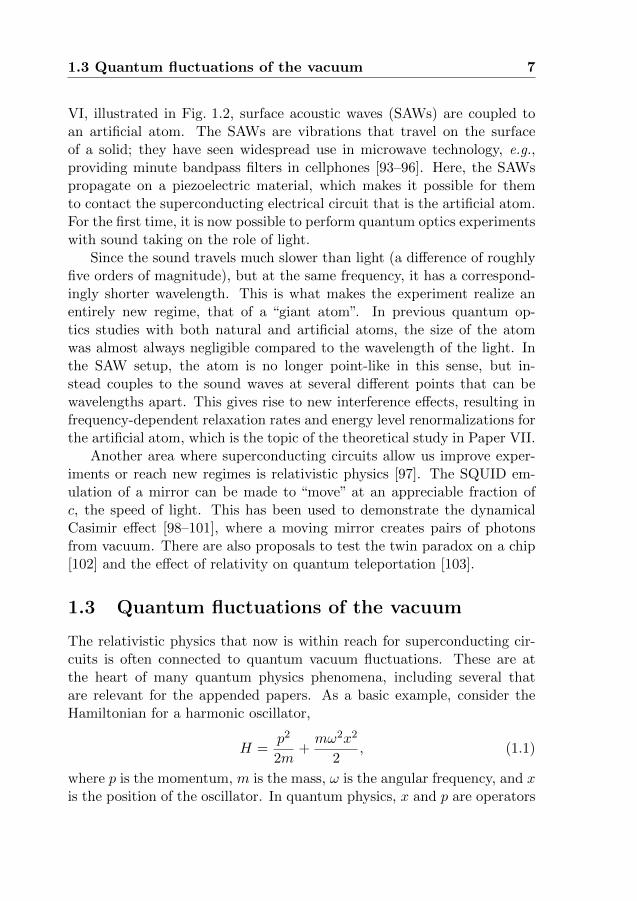
VI, illustrated in Fig. 1.2, surface acoustic waves (SAWs) are coupled toan artificial atom. The SAWs are vibrations that travel on the surfaceof a solid; they have seen widespread use in microwave technology, e.g.,providing minute bandpass filters in cellphones [93–96]. Here, the SAWspropagate on a piezoelectric material, which makes it possible for themto contact the superconducting electrical circuit that is the artificial atom.For the first time, it is now possible to perform quantum optics experimentswith sound taking on the role of light.

Since the sound travels much slower than light (a difference of roughlyfive orders of magnitude), but at the same frequency, it has a correspond-ingly shorter wavelength. This is what makes the experiment realize anentirely new regime, that of a “giant atom”. In previous quantum op-tics studies with both natural and artificial atoms, the size of the atomwas almost always negligible compared to the wavelength of the light. Inthe SAW setup, the atom is no longer point-like in this sense, but in-stead couples to the sound waves at several different points that can bewavelengths apart. This gives rise to new interference effects, resulting infrequency-dependent relaxation rates and energy level renormalizations forthe artificial atom, which is the topic of the theoretical study in Paper VII.

Another area where superconducting circuits allow us improve exper-iments or reach new regimes is relativistic physics [97]. The SQUID em-ulation of a mirror can be made to “move” at an appreciable fraction ofc, the speed of light. This has been used to demonstrate the dynamicalCasimir effect [98–101], where a moving mirror creates pairs of photonsfrom vacuum. There are also proposals to test the twin paradox on a chip[102] and the effect of relativity on quantum teleportation [103].

1.3 Quantum fluctuations of the vacuum

The relativistic physics that now is within reach for superconducting cir-cuits is often connected to quantum vacuum fluctuations. These are atthe heart of many quantum physics phenomena, including several thatare relevant for the appended papers. As a basic example, consider theHamiltonian for a harmonic oscillator,

H = p2

2m + mω2x2

2 , (1.1)

where p is the momentum, m is the mass, ω is the angular frequency, and xis the position of the oscillator. In quantum physics, x and p are operators

8 Introduction

with the commutation relation [x, p] = i~, where ~ = h/2π (h is Planck’sconstant). Using this, and defining the annihilation and creation operators

a =√mω

2~

(x+ ip

mω

), (1.2)

a† =√mω

2~

(x− ip

mω

), (1.3)

the Hamiltonian can be rewritten as [104]

H = ~ω(a†a+ 1

2

). (1.4)

The operator a†a counts the number of excitations of the oscillator. Wesee that even if the oscillator is in its ground state (zero excitations), itstill has an energy ~ω

2 . This is the vacuum energy; the oscillator is nevercompletely still.

The electromagnetic field can be described as a collection of harmonicoscillators where the excitations are photons [105, 106]. Thus, in the elec-tromagnetic vacuum there are photons flitting in and out of existence,which leads to several interesting effects. One example is the static Casimireffect [107], where two stationary mirrors in vacuum experience an attrac-tive force due to there being fewer allowed electromagnetic field modesbetween them than elsewhere. The Casimir force is a result of more vac-uum fluctuations pushing from the outside than from the inside. Thiseffect has been detected experimentally [108]. Vacuum effects in relativis-tic settings include the dynamical Casimir effect mentioned above as wellas Hawking radiation [109] and the Unruh effect [110].

The presence of vacuum fluctuations also affects atoms. A well-knownexample is the Lamb shift [111, 112], a renormalization of energy levels inthe hydrogen atom. This kind of shift has also been measured for artifi-cial atoms in superconducting circuits [113] and we calculate it for a giantartificial atom in Paper VII. Another effect of the vacuum fluctuations isthat they induce relaxation of excited atom states [105, 114–116]. Thisis the quantum version of the fluctuation-dissipation theorem, which con-nects random fluctuations in the environment of a system with dissipationfrom that system [117–119]. Dissipation from a quantum system to anenvironment occurs in all the appended papers.

In Paper VIII, we use an artificial atom to map out the structure ofvacuum fluctuations in front of a mirror (the end of a transmission line), as

1.4 Quantum computing and parity measurement 9

Figure 1.3: Sketch of an artificial atom probing quantum vacuum fluctuations infront of a mirror. The superconducting circuit that is the artificial atom is placedat a distance L from the termination of a transmission line to ground, which isan effective mirror. By modulating the transition frequency ωa of the atom, thedistance to the mirror can be changed in terms of wavelengths λ = 2πc/ωa, wherec is the speed of light in the transmission line. Changing the effective distance L/λplaces the atom at a node (blue line) or antinode (red line) of vacuum fluctuationmodes.

illustrated in Fig. 1.3. The information is extracted by measuring the re-laxation rate of the atom as we tune its frequency, thus effectively changingits distance to the mirror.

Finally, quantum fluctuations of the vacuum are also important in thecontext of measurements on quantum systems [120]. The fluctuations re-sult in an unavoidable noise background, which must be overcome. This isa vital point for the different measurement schemes analyzed in Papers I,II, and V.

1.4 Quantum computing and parity measurement

We have already alluded to the building of a quantum computer as animportant motivation for much of the development in quantum optics inthe last decades. The idea of a quantum computer was introduced byFeynman in 1982 [121]. In contrast to a classical computer, which operatesusing bits that can be in the two states 0 and 1, a quantum computer wouldwork with quantum bits, qubits. Qubits have eigenstates denoted |0〉 and|1〉, but they can exist in a superposition of these states,

|ψ〉 = α |0〉+ β |1〉 , (1.5)

where α and β are complex numbers satisfying the normalization condition|α|2 + |β|2 = 1 [122]. Such a superposition state can be represented on a

10 Introduction

Figure 1.4: The Bloch sphere representation of a qubit. The basis states arelocated at the north and south poles. The various possible superpositions of thetwo can then be converted to unique coordinates on the sphere, since an equivalentparametrization of the superposition is |ψ〉 = cos θ2 |0〉+ eiφ sin θ

2 |1〉.

Bloch sphere, shown in Fig. 1.4.

Simply put, the possibility of putting a qubit in superposition statesenables a parallelization of computation that provides an advantage com-pared to classical computers. Several quantum computing algorithms havebeen developed that can provide a great speed-up for solving certain classesof problems [123–127].

To build a fully working quantum computer, an architecture must befound that is scalable and uses long-lived qubits that can both be measuredand work in gate operations [128]. Several systems, with both natural andartificial atoms, are being investigated for this purpose [16, 26, 28, 129–133]. However, so far only a few qubits have been made to work together[134–137] (not counting the D-Wave machines [138–144]). Hence, beforewe see large-scale quantum computers we will first have quantum simula-tors [145–152], where a smaller number of qubits are used to investigatequantum physics problems that are intractable on classical computers; ittakes 2N classical bits to simulate N quantum two-level systems, but itonly takes N qubits.

It is also hard to make qubits that can maintain a superposition statefor a long time. Coupling to environmental noise like vacuum fluctuations

1.4 Quantum computing and parity measurement 11

Encoding Measurements Correction

|ψ〉 • •Bitfliperror

M12Flip iff M12 = −1,M23 = 1

|0〉M23

Flip iff M12 = −1,M23 = −1

|0〉 Flip iff M12 = 1,M23 = −1

Figure 1.5: A circuit diagram for the three-qubit bit-flip error-correction code. Inthe first step, quantum controlled-NOT (CNOT) gates are applied to produce thestate |ψ3〉 from |ψ〉 (see Eq. (1.6)). After a bit-flip error occurs, parity measure-ments are done and correcting flips are applied to the qubits depending on themeasurement results (-1 means the qubits are in opposite states, +1 that they arein the same state).

leads to decoherence of the qubit. For superconducting qubits there hasbeen tremendous progress in the last few years, increasing coherence timesfrom microseconds to above a millisecond [153–155]. This is not enough initself to enable computations with low enough error rate, but it is at thethreshold for being useful in quantum error correction codes, where severalqubits together represent and store the information of a single “logicalqubit” [156–159]. This redundancy allows for a kind of “majority vote”system where if one qubit fails, that can be detected and corrected usingthe others.

In the last years, 2D surface codes have emerged as a good, scalablecandidate for error correction in quantum computing [160, 161]. These andother codes use parity measurements to detect errors without disturbingthe encoded logical qubit. A parity measurement on two or more qubits isa measurement which determines whether an even or odd number of themare in the same state. The measurement does not give any informationabout the states of the individual qubits, preserving their superpositionstates. Thus a parity measurement on two qubits tells us if they are ineither some superposition of |00〉 and |11〉 or in some superposition of |01〉and |10〉. It does not give us any clue about whether any single qubit is instate |0〉 or |1〉.

The simple three-qubit code, which can protect against bit-flip errors,is a pedagogical example showing how parity measurements can be usedin error correction [122] (and has been implemented with superconductingcircuits [162]). The process is shown schematically in Fig. 1.5. We take

12 Introduction

our logical state |ψ〉 from Eq. (1.5) and encode it using three qubits as

|ψ3〉 = α |000〉+ β |111〉 . (1.6)

It is important to note that the quantum no-cloning theorem [163, 164]prevents us from merely creating three independent identical copies of |ψ〉;we have to make this entangled state instead. Now, let us assume that thethird qubit is flipped. This gives

|ψ3,err〉 = α |001〉+ β |110〉 . (1.7)

If we first do a parity measurement on qubits 1 and 2, and then on qubits2 and 3, we do not affect the state |ψ3,err〉. However, the result of themeasurements lets us draw the conclusion that qubit 3 has been flipped(assuming that the probability of more than one qubit flipping is negligi-ble). We can then apply a control pulse to this qubit, flipping it back toits original state.

In Paper I, we show how parity measurements in circuit QED can beimproved by undoing unwanted measurement back-action. The setup weinvestigate has two qubits coupled to a resonator. By driving the resonatorwith a coherent microwave signal, and detecting the output in a suitableway, one can for certain system parameters realize a parity measurement ofthe two qubits [165]. However, the measurement also seems to give extraback-action on one of the parity states, which would make it unsuitable forpractical use. In our paper, we are able to show that a careful analysis ofthe measurement signal reveals all the information about this extra back-action needed to undo it.

1.5 Overview of the thesis

This is a compilation thesis, consisting of an introductory text and ap-pended reprints of eight papers. In the present chapter, we have givenan overview of the field, placing the work of the appended papers in theirproper context and explaining the motivation for them. In the next fewchapters, we will mainly review the theoretical tools used in the appendedpapers. Although some of the appended papers include experiments, this isa theory thesis, and we defer to the appended papers in question, togetherwith the theses of some of our experimental collaborators [40, 166–168],for details about fabrication and measurement setups.

1.5 Overview of the thesis 13

Chapter 2 is devoted to the various components of the systems we con-sider in the appended papers: transmission lines, surface acoustic waves,and artificial atoms in the form of superconducting qubits. We review howto formulate a quantum mechanical description of such electrical circuitsand say a few words about the Jaynes–Cummings model, which describesinteraction between an atom and a resonator.

Chapters 3–5 form the theoretical backbone of the thesis. In Chapter 3,we begin to look at open quantum systems, where a small quantum systemis coupled to an environment with a large number of degrees of freedom. Tohandle this situation, master equations are introduced which constitute aneffective description of the system under the influence of the environment.This is used to some extent in all appended papers. From the masterequation we then move on to input-output theory, which deals in moredetail with excitations arriving at and leaving the small system.

The output from a system can be measured in various ways; this isthe topic of Chapter 4. It is especially important for Papers I, II, and V,which deal with both parity measurements and photon detection. In thesepapers, as well as in Papers VII and VIII, we also make use of the (S,L,H)formalism for cascaded quantum systems, which is the topic of Chapter 5.Here, input-output theory is extended to handle output from one systembeing used as input for another.

Chapter 6 is an overview of the results in the appended papers. Briefly,Paper I analyzes a scheme for parity measurement in circuit QED andshows that an unwanted type of measurement back-action actually can beavoided by fully using the information in the measurement record. PapersII and V are theoretical investigations of a possible photon detector setupfor circuit QED, where artificial atoms mediate an interaction betweenthe photon to be detected and a coherent probe signal. In Paper II, weshow that one atom is not enough to overcome the quantum backgroundnoise, but Paper V shows that several atoms cascaded in the right way cando it. Paper III is a proof-of-principle experiment demonstrating that anartificial atom in the form of a superconducting circuit can indeed mediatethe strong photon-photon interactions we rely on in Papers II and V.

In Paper IV, we explain experimental results for an artificial atomcoupled to photons in a resonator. The system exhibits rich dynamicswhen driven and probed with signals at different frequencies. Finally,Papers VI, VII, and VIII are all concerned with an artificial atom coupledto a bosonic field at several points, which can be wavelengths apart. In

14 Introduction

Paper VIII, an artificial atom placed in front of a mirror is used as a probeof the interference pattern in the mode structure of the quantum vacuumfluctuations. Paper VI is a ground-breaking experimental demonstrationof coupling between an artificial atom and propagating sound in the formof SAWs. The short wavelength of the SAWs makes the atom “giant” incomparison; the effects of this new regime is explored further theoreticallyin Paper VII, which shows how the multiple coupling points of the atomgive rise to interference effects affecting both the atom’s relaxation rateand its energy levels.

Finally, we conclude in Chapter 7 by summarizing our work and lookingto the future. There are indeed many interesting directions to pursue inthe field of quantum optics with artificial atoms.

Chapter 2

Artificial atoms and 1Dwaveguides

As we saw in Chapter 1, there are many systems that can be used for ex-periments in quantum optics. The archetypical setup is either single atomsor ions, trapped in an electromagnetic field, being manipulated with laserlight [2, 4, 11–13, 15, 129, 135, 136, 148, 169, 170], or the reverse, lighttrapped between two mirrors interacting with passing atoms [2, 3, 5–8, 18,19, 171, 172]. However, in the last decade or so, an increasing numberof quantum optics experiments have been done using artificial atoms insuperconducting circuits [23–28, 35, 37, 41, 101, 113, 137, 162]. The versa-tility offered by superconducting circuits in designing the artificial atomsand their couplings to the surroundings, as well as the simplicity of usingexisting microwave technology for the signal processing in experiments, arethe main reasons behind this development.

Since all experimental papers in this thesis use superconducting cir-cuits, and all the theoretical papers are written mainly with such imple-mentations in mind, this chapter is devoted to the quantum theory ofelectrical circuits. After we introduce the theoretical tools needed to gofrom a classical circuit description to a quantum one, we will illustratetheir use on our two main components: the transmission line and the ar-tificial atom known as a transmon [173]. We will also look at theory forsurface acoustic waves in piezoelectric materials and show how a transmoncan couple to such waves. Finally, we say a few words about regimes inthe Jaynes–Cummings model [174], which describes interactions betweenan atom and photons in a resonator.

16 Artificial atoms and 1D waveguides

2.1 Circuit QED

The process for quantizing circuits has already been well described inRefs. [175–179]. In the following, we will cover the main points in thesereferences.

To arrive at a quantum description given an electrical circuit, the firststep is to write down the classical Lagrangian L [180] of the circuit. Itturns out to be convenient to work with node fluxes

Φn(t) =∫ t

−∞Vn(t′) dt′, (2.1)

where Vn denotes node voltage at node n, and node charges

Qn(t) =∫ t

−∞In(t′) dt′, (2.2)

where In denotes node current. With the node fluxes as our generalizedcoordinates, the Hamiltonian H follows from the Legendre transformation[180]

H =∑

n

∂L

∂ΦnΦn − L. (2.3)

The generalized momenta ∂L∂Φn

will sometimes, but not always, be the node

charges Qn.Up to this point, everything has been completely classical. To pro-

ceed to quantum mechanics, we promote the generalized coordinates andmomenta to operators with the canonical commutation relation

[Φn,

∂L

∂Φm

]= i~δnm, (2.4)

where δnm is the Kronecker delta.For quantum optics with superconducting circuits, three basic elements

are needed: capacitors, inductors, and Josephson junctions, illustrated inFig. 2.1. A Josephson junction consists of a thin insulating barrier betweentwo superconducting leads, and it can be modelled as a capacitor in parallelwith a nonlinear inductor characterized by the Josephson energy EJ.

The Lagrangians for capacitors and inductors are straightforward. Theenergy of a capacitor with capacitance C is

CV 2

2 =C(Φ1 − Φ2

)2

2 , (2.5)

2.1 Circuit QED 17

C L EJ CJ

Φ1

Φ2

Φ1

Φ2

Φ1

Φ2

Figure 2.1: The three basic circuit elements used in quantum optics for supercon-ducting circuits. From left to right: capacitance C, inductance L, and a Josephsonjunction with capacitance CJ and Josephson energy EJ.

where V is the voltage across the capacitor, and for an inductor withinductance L it is

LI2

2 =V = LI

= (Φ1 − Φ2)2

2L , (2.6)

where I is the current through the inductor. In the Lagrangian, capacitiveterms (terms with Φ) represent kinetic energy and give a positive contribu-tion, while inductive terms (terms with Φ) represent potential energy andgive a negative contribution. We thus have

LC =C(Φ1 − Φ2

)2

2 , (2.7)

LL = −(Φ1 − Φ2)2

2L . (2.8)

For the Josephson junction, the contribution from the capacitive partwith CJ follows immediately from previous discussion. To get the contri-bution from the nonlinear inductor, we use the Josephson equations [29,30]

IJ = IC sinφ, (2.9)

φ = 2e~V (t), (2.10)

where IJ is the supercurrent through the junction, IC is the critical cur-rent (the maximum value of IJ), V (t) is the voltage across the junction,φ = 2e (Φ1 − Φ2) /~ is a phase difference across the junction, and e is theelementary charge. These equations give

∫ t

−∞I(t′)V (t′) dt′ = EJ (1− cosφ) , (2.11)


C0∆x

L0∆x

C0∆x

L0∆x

C0∆x

Φn−1 Φn Φn+1

︸︷︷︸∆x

Figure 2.2: Circuit diagram for a transmission line. C0 and L0 denote capacitanceper unit length and inductance per unit length, respectively, and ∆x is a smalldistance which will go to zero in the continuum limit.

where we have identified the Josephson energy EJ = ~IC/2e. The La-grangian for the Josephson junction is thus

LJJ =CJ

(Φ1 − Φ2

)2

2 − EJ (1− cosφ) . (2.12)

Note that the inductive term is a cosine function rather than the quadraticfunction for a normal inductor; this is why the Josephson junction can beseen as nonlinear inductance. This nonlinearity is essential for makingartificial atoms with different level structures. From normal capacitorsand inductors we can only get harmonic LC-oscillators.

2.2 The quantized transmission line

With the formalism for quantum circuits in hand, we now apply it to ourfirst building block in quantum optics with superconducting circuits: thetransmission line. A microwave transmission line is basically a coaxialcable squashed onto a chip; it consists of a center conductor between twoground planes. We will first consider an infinitely long transmission lineand then insert mirrors (gaps) to form resonators.

2.2.1 The infinite 1D waveguide

The transmission line can be modelled by the circuit depicted in Fig. 2.2[181, 182]. Using Eqs. (2.7) and (2.8), we immediately get the Lagrangian

LTL =∑

n

[C0∆x

2(Φn(t)

)2− 1

2L0∆x(Φn+1(t)− Φn(t))2

], (2.13)

2.2 The quantized transmission line 19

from which we can identify the conjugate momenta

∂LTL

∂Φn= C0∆xΦn(t), (2.14)

which are the node charges Qn(t). Applying the Legendre transformation(Eq. (2.3)) to LTL, inserting the definition of the node charges, and takingthe limit ∆x→ 0 (or rather ∆x→ dx) gives the Hamiltonian

HTL = 12

∫ ∞

−∞dx(Q(x,t)2

C0+ 1L0

(∂Φ(x,t)∂x

)2), (2.15)

where Q(x,t) and Φ(x,t) are charge density and flux density, respectively.The Lagrangian can also be written in a continuum form

LTL =∫ ∞

−∞dxL =

∫ ∞

−∞dx(C02(Φ(x,t)

)2− 1

2L0

(∂Φ(x,t)∂x

)2), (2.16)

and applying the Euler-Lagrange equations [106]

∂

∂µ

∂L∂(∂Φ∂µ

)

− ∂L

∂Φ= 0, µ = x,t (2.17)

to the Lagrangian density L gives the wave equation

∂2Φ(x,t)∂t2

− 1L0C0

∂2Φ(x,t)∂x2 = 0. (2.18)

This tells us that there will be left- and right-moving flux waves

Φ(x,t) = ΦL(kx+ ωt) + ΦR(−kx+ ωt) (2.19)

moving in the transmission line with velocity v = 1/√L0C0 and wavenum-

ber k = ω/v.So far, all calculations have been classical. To quantize the field in the

transmission line, we promote the generalized coordinates and momentato operators with the commutation relation

[Φ(x), Q(x′)

]= i~δ(x− x′), (2.20)

where the delta function, rather than the Kronecker delta, appears since weare working with a continuum model. From the form of the Hamiltonian in


Eq. (2.15) it can be seen that we have a collection of harmonic oscillators.We can thus rewrite the generalized coordinates and momenta in termsof annihilation and creation operators, just like in Sec. 1.3. The left- andright-moving fluxes become [175, 178, 183]

ΦL/R(x,t) =√

~Z04π

∫ ∞

0

dω√ω

(aL/R,ωe

−i(±kx+ωt) + H.c.), (2.21)

where H.c. denotes Hermitian conjugate, the annihilation and creation op-erators obey the commutation relations

[aX,ω, a

†X’,ω′

]= δ(ω − ω′)δXX′ , (2.22)

and Z0 =√L0/C0 is the characteristic impedance of the transmission line.

To connect to the discussion of quantum vacuum fluctuations in Sec. 1.3and the measurement of their strength in a semi-infinite transmission linein Paper VIII, it is illustrative to calculate the spectral density of thevoltage fluctuations in our open transmission line using Eq. (2.21). UsingV = ∂tΦ, we have [120]

SV V [ω] =∫ ∞

−∞dteiωt 〈V (t)V (0)〉

=∫ ∞

−∞dteiωt~Z0

4π

∫ ∞

0

dω′√ω′

∫ ∞

0

dω′′√ω′′

(−iω′)(−iω′′)

×⟨(

aL,ω′e−i(kx+ω′t) + aR,ω′e−i(−kx+ω′t) −H.c.)

×(aL,ω′′e−ikx + aR,ω′′eikx −H.c.

)⟩

= ~Z04π

∫ ∞

−∞dteiωt

∫ ∞

0dω′√ω′∫ ∞

0dω′′√ω′′2e−iω′tδ(ω′ − ω′′)

= ~Z02π

∫ ∞

0dω′ω′2πδ(ω − ω′) = Z0~ω, (2.23)

where we assumed negligible temperature such that the only contribution

from the expectation value is terms on the form⟨aa†

⟩= 1. The result

shows that the left- and right-travelling modes each contribute ~ω/2 to thepower spectral density SV V [ω]/Z0, which agrees well with our expectationsfor the quantum vacuum fluctuations.

2.2 The quantized transmission line 21

2.2.2 Mirrors and resonators

We can now proceed to introduce boundary conditions in the open trans-mission line. Grounding one end at x = 0 gives the boundary conditionΦ(0,t) = 0; it is equivalent to inserting a mirror in open space. It is alsopossible to connect one end of the transmission line to ground via a capac-itance or via a SQUID (the latter gives a tunable boundary condition, amoving mirror, as discussed in Sec. 1.2).

A semi-infinite transmission line still has a continuum of modes, but theboundary condition gives rise to a mode structure. This can be seen as aninterference effect between waves approaching the mirror and waves thathave been reflected off the mirror. In Paper VIII, we explore this modestructure, which is imposed also on the vacuum fluctuations, by placingan artificial atom close to a mirror and varying its resonance frequency.The relaxation rate of the atom is proportional to the spectral density ofthe voltage fluctuations at the atom transition frequency, which given theboundary condition Φ(0,t) = 0 becomes SV V [ω]/Z0 = 2~ω sin2(kx).

A semi-infinite transmission line is also used in the experiment of PaperIII, where a three-level artificial atom placed close to a mirror is used tomediate photon-photon interactions. Here, the main point of using themirror is to give unidirectionality that improves efficiency; all the photonsmust go out in one direction, whereas in an open transmission line theycan be scattered by the atom in two different directions.

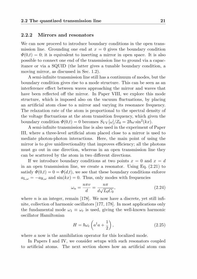
If we introduce boundary conditions at two points x = 0 and x = din an open transmission line, we create a resonator. Using Eq. (2.21) tosatisfy Φ(0,t) = 0 = Φ(d,t), we see that these boundary conditions enforceaL,ω = −aR,ω and sin(kx) = 0. Thus, only modes with frequencies

ωn = nπv

d= nπ

d√L0C0

, (2.24)

where n is an integer, remain [178]. We now have a discrete, yet still infi-nite, collection of harmonic oscillators [177, 178]. In most applications onlythe fundamental mode ω1 ≡ ωr is used, giving the well-known harmonicoscillator Hamiltonian

H = ~ωr

(a†a+ 1

2

), (2.25)

where a now is the annihilation operator for this localized mode.In Papers I and IV, we consider setups with such resonators coupled

to artificial atoms. The next section shows how an artificial atom can


Cg

+−VgEJ CJ

Φ

Figure 2.3: Circuit diagram for a Cooper-pair box. The Josephson junction ismodelled by the capacitance CJ in parallel with a nonlinear inductor havingJosephson energy EJ. The node between the gate capacitance Cg and the Joseph-son junction is called the ”island”.

be constructed from superconducting circuits, and Sec. 2.5 explores theHamiltonian that results from the interaction between an atom and a res-onator.

2.3 The transmon qubit

There are several ways to build an artificial atom with superconducting cir-cuits [27, 178, 184–190]. Their common denominator is the use of Joseph-son junctions to provide a nonlinear element. In this section, we will givean overview of one implementation, the transmon [173], which is used orconsidered in all the appended papers of this thesis.

The transmon is a variation on the Cooper-pair box (CPB) [185, 186,191], the circuit diagram of which is shown in Fig. 2.3. The CPB consistsof a small superconducting island connected to a superconducting reservoirvia a Josephson junction, which allows Cooper pairs to tunnel on and offthe island. The model also includes an external voltage source Vg coupledto the island via a gate capacitance Cg, to determine the background chargeng = CgVg/2e (measured in units of Cooper pairs) that the environmentinduces on the island.

Using Eqs. (2.7) and (2.12) we get the CPB Lagrangian

LCPB =Cg

(Φ− Vg

)2

2 + CJΦ2

2 − EJ(1− cos 2eΦ~

) (2.26)

Applying the Legendre transformation, identifying the conjugate momen-tum (the node charge) Q = (CJ + Cg)Φ − CgVg, and removing constant

2.3 The transmon qubit 23

−1 −0.5 0 0.5 1

0

0.5

1

1.5

2

ng

Energy

−1 −0.5 0 0.5 1

0

0.5

1

1.5

2

ng

Figure 2.4: The three lowest energy levels of a CPB plotted as a function of ng forEJ/EC = 1 (left) and EJ/EC = 20 (right). The energy scale is normalized to thelevel separation between the ground state and the first excited state at ng = 0.The decreased sensitivity to charge noise in the transmon regime (EJ/EC 1),as well as the decreased anharmonicity, is apparent.

terms that do not contribute to the dynamics, we arrive at the Hamiltonian

HCPB = 4EC(n− ng)2 − EJ cosφ, (2.27)

where EC = e2/2(Cg + CJ) is the electron charging energy, n = −Q/2e isthe number of Cooper pairs on the island, and φ = 2eΦ/~.

We now promote Φ and Q to operators in the same way as in theprevious sections. This translates into a commutation relation for n andφ, which since the Hamiltonian is periodic in φ should be expressed as [105,179] [

eiφ, n]

= eiφ. (2.28)

From this follows that e±iφ |n〉 = |n∓ 1〉, where |n〉 is the charge basiscounting the number of Cooper pairs. Using the resolution of unity [104]and cosφ = (eiφ+e−iφ)/2 we can then write the Hamiltonian in the chargebasis as [177, 178]

HCPB =∑

n

[4EC(n− ng)2 |n〉〈n| − 1

2EJ (|n+ 1〉〈n|+ |n− 1〉〈n|)].

(2.29)The energy level structure of HCPB depends on the parameters EJ, EC,

and ng. As ng represents the influence of the environment, we would likeit to have little effect in order to have a stable, controllable system. This isachieved when EJ EC (the phase rather than the charge dominates), as


is illustrated in Fig. 2.4. The price to be paid is a decrease in anharmonic-ity, i.e., the difference between the transition energy needed to go from theground state to the first excited state and the transition energy needed togo from the first excited state to the second excited state. To work as aqubit, an artificial atom has to be anharmonic enough to be approximatedas a two-level system when driving the first transition; a signal driving theatom from the ground state to the first excited state should not be ableto induce a further transition to the second excited state. Fortunately,the influence of ng decays much faster than the anharmonicity when EJ isincreased, so the transmon can indeed be used as a qubit [173].

In the limit EJ EC, the energy levels of the transmon are approxi-mately given by [173]

Em = −EJ +√

8EJEC

(m+ 1

2

)− EC

12(6m2 + 6m+ 3

). (2.30)

From this, we get the anharmonicity

α = E2,1 − E1,0 = (E2 − E1)− (E1 − E0) = −EC . (2.31)

Since EC EJ, the anharmonicity is small compared to the transitionfrequencies, but it can still be large enough compared to drive strengths andrelaxation rates in the system to ensure that the transmon can be operatedas a two-level system. To achieve a low EC, one adds a shunt capacitance inparallel with CJ, often by designing the transmon in the form of two islandsthat form an interdigitated finger structure with high capacitance. Theislands are usually connected by a SQUID (see Sec. 1.2) rather than a singleJosepshon junction. The SQUID functions as a Josephson junction with atunable EJ (controlled by the magnetic flux through the SQUID), whichmeans that the energy levels and transition frequencies of the transmoncan be tuned in situ during an experiment.

The transmon is not always operated as a pure two-level system. Insome cases, the second excited state of the transmon is actually used toimplement qubit gates [162, 192, 193]. Indeed, d-level systems, qudits,make quantum computation possible with less resources [194–196] and cansimulate more quantum systems than qubits [197]; transmons seem wellsuited to work as qudits [198, 199]. Another advantage of the transmon isthat the superconducting island shape can be designed to couple to severalother transmons or resonators [200, 201].

2.4 Surface acoustic waves 25

2.4 Surface acoustic waves

While most papers in this thesis are concerned with transmons coupled tophotons in electric transmission lines, Paper VI shows that a transmon canalso interact with phonons in the form of surface acoustic waves. In thissection, we will first review classical theory for SAWs and then show howthey couple to a transmon.

2.4.1 Classical SAW theory

Surface acoustic waves are a type of vibrations in a solid that are confinedto the surface of the material, decaying exponentially in the bulk. Suchsolutions to the wave equation in a 3D material were first found by LordRayleigh in 1885 [202] and they are important in many natural phenom-ena, e.g, in earthquakes. About 50 years ago, it was realized that SAWs inpiezoelectric materials can be used to convert long-wavelength electromag-netic radiation to short-wavelength vibrations, which has proven extremelyuseful in TV and cellphone technology [93–96]. Here, we will mainly followRef. [93] to explain the basic mechanisms.

Applying a force F to a 3D solid material can give rise to particledisplacements u. To describe this, one defines the stress tensor

Tij = FiAj, i,j = x,y,z, (2.32)

where Fi is the force in direction i and Aj is the cross-section area indirection j (the area vector is taken as the normal pointing outwards fromthe volume under consideration). The stress gives rise to a strain

Sij = ∂ui∂j

, i,j = x,y,z, (2.33)

which measures the fractional change of length in the material. The stressand the strain are related by an elasticity tensor, or stiffness coefficient,

Tij = cijklSkl. (2.34)

From symmetry considerations it is possible to show that Tij = Tji, reduc-ing the number of independent stresses to six. These can be gathered in avector

T = (Txx, Tyy, Tzz, Tyz, Tzx, Txy). (2.35)


Similarly, we can define a strain vector S, where the last three entries aresymmetrizations,

S = (Sxx, Syy, Szz, Syz + Szy, Sxz + Szx, Sxy + Syx) . (2.36)

We are then left withT = cS, (2.37)

where c is a 6× 6 stiffness matrix.For a dielectric material, there is a similar relation between an applied

electric field E and the electrical displacement D,

D = εE, (2.38)

where ε is a 3 × 3 permittivity matrix. In most materials, the processesof Eqs. (2.37) and (2.38) are independent of each other. However, in apiezoelectric material, the arrangement of the atoms is such that a strainwill give rise to a polarization charge, and vice versa. The result is thatwe get two coupled equations,

T = cS− eTE, (2.39)

D = eS + εE, (2.40)

where e is a 3× 6 matrix known as the piezoelectric constant and eT is itstranspose. To see the interplay between electricity and vibrations, we willconsider as an example a compressional wave moving in the x direction ina material with e11 6= 0. Eqs. (2.39)-(2.40) then become

T1 = c11S1 − e11E1, (2.41)

D1 = e11S1 + ε11E1. (2.42)

Following Ref. [93], we will now connect to Sec. 2.2, showing that this ex-ample is equivalent to a transmission line. To see this, we first introducethe particle displacement velocity v = ∂tu (we drop subscripts from hereon). Since S = ∂xu, taking the time derivative of Eq. (2.41) and rearrang-ing the terms gives

∂v

∂x= 1c

∂T

∂t+ e

c

∂E

∂t. (2.43)

Then, solving Eq. (2.39) for S, inserting the result into Eq. (2.40), solvingthe resulting equation for E and inserting that result in Eq. (2.43) leadsto

∂v

∂x= 1c′∂T

∂t+ e

εc′∂D

∂t, (2.44)


where we have defined

c′ = c+ e2

ε≡ c(1 +K2). (2.45)

K2 = e2/εc is called the electromechanical coupling ; it is a defining prop-erty for piezoelectric materials. In the most strongly piezoelectric materi-als, like lithium niobate (LiNbO3), K2 ≈ 5 · 10−2, while gallium arsenide(GaAs), which was used in the experiment of Paper VI, has K2 ≈ 7 · 10−4.

In the quasi-electrostatic approximation, D is constant (assuming thatthe material has no free charges and that there is external voltage applied).With this and the definition in Eq. (2.32), Eq. (2.44) becomes

∂v

∂x= 1c′A

∂F

∂t(2.46)

for a cross-section area A.

To get a second equation that will help us connect this to a trans-mission line model, we consider the effect of stress on an infinitesimalcube with sides dx, dy, and dz, having mass density ρm. On one side ofthe cube, there is a force Tdydz, while on the opposite side the force is(T + (∂xT ) dx) dydz. Newton’s second law, F = ma, used on the net forcegives

∂T

∂xdxdydz = ρmdxdydz ∂v

∂t, (2.47)

which can be rewritten as

∂F

∂x= ρmA

∂v

∂t. (2.48)

Eqs. (2.46) and (2.48) are of the same form as the equations for voltageV and current I in a transmission line,

∂V

∂x= −L0

∂I

∂t, (2.49)

∂I

∂x= −C0

∂V

∂t. (2.50)

Making the identifications

V ↔ −F, I ↔ v, L0 ↔ ρmA, C0 ↔1c′A

, (2.51)


Figure 2.5: SAW propagation on a substrate. The particle motion includes bothcompression in the x direction, which is the propagation direction of the SAW,and shearing in the y direction.

we can thus extract the acoustic wave propagation velocity

vwave = 1√L0C0

= 1√ρmA

1c′A

=√

c′

ρm. (2.52)

The example above was for an acoustic wave moving in the bulk ofa piezoelectric material. A surface acoustic wave is more complicated, asshown in Fig. 2.5. If we let x be the propagation direction (the surface isthe xz plane), the SAW will include compressional motion in the x directionand shearing in the y direction (this gives in total elliptical particle motion),along with an electrostatic wave. Since we are interested in connecting toelectronics, it is convenient to make the electric potential at the surface, φ,our main variable. Given φ, ux and uy will be fixed by material parameters.

The full SAW description involves permittivities and piezoelectric cou-plings in several directions as well as an exponentially decaying part in they direction. With the reasonable approximations that the compressionalmotion dominates and that the electrostatic part is described by the con-stant potential φ in a shallow layer at the surface (zero elsewhere), it isstill possible to use a transmission line picture. The potential φ is thenequated to the voltage V in the transmission line and a transmission lineconductance Y0 is defined such that the total power carried by the SAW,including both electrical and mechanical contributions, is

P = Y0 |φ|2 . (2.53)


Figure 2.6: A sketch of an IDT. Two islands with periodically spaced metal fingersof length W are connected to a voltage source VT. The voltage induces strain inthe piezoelectric substrate, launching SAWs to the left and right with electricpotential φL/R.

Since the conductance will depend on the width W of the SAW, a charac-teristic conductance y0 is defined using the SAW wavelength λ,

y0 = λ

WY0. (2.54)

From calculations similar to those of the example above, but with somemore care taken to reflect that we are now at a surface, it can be shownthat [93]

y0 = 2πCsv0K2 , (2.55)

where v0 is the SAW propagation velocity and Cs = ε0 + εp (εp being thepermittivity of the substrate and ε0 the permittivity of the medium abovethe substrate).

With a theory for SAW propagation in place, the next step is to gen-erate the waves. Current SAW technology is based on the interdigitaltransducer (IDT), invented in 1965 [203]. An IDT consists of a num-ber of metallic fingers placed periodically on the piezoelectric substrate assketched in Fig. 2.6. When an AC voltage VT is applied to the transducer,it induces strain in the piezoelectric substrate and generates SAWs withamplitude φ = µVT, where µ is a coupling constant that will be determined


shortly. Conversely, a SAW wave arriving at the IDT structure will gener-ate a current I = gmφ. The reciprocity between conversion from electricalsignal to SAW and vice versa leads to a relation between gm and µ [93]:

gm = 2µY0, (2.56)

where the factor 2 comes from the applied voltage generating waves withamplitude µVT in each propagation direction (both to the left and to theright).

To calculate µ for a single IDT finger pair of length W , we can ap-proximate it as a capacitor with capacitance WCs and a uniform chargedensity set by VT . This acts as a current source in the SAW transmissionline; the result is [93]

µ = icgK2, (2.57)

where cg is a geometry factor on the order of 1. Its exact value dependson the metallization ratio η, the ratio between the finger width a and theinter-finger distance p. The result in Eq. (2.57) also assumes that we areconsidering a frequency matching the resonance condition λ = 2p.

For the case of multiple fingers, one simply sums the individual fingercontributions, including the phase shift the SAW acquires travelling fromone finger to the next. If we, for convenience, ground one of the electrodesand let the coordinates of the Np fingers of the other electrode be xk, weget

|µ| = cgK2

∣∣∣∣∣∣

Np∑

k=1ei2πfxk/v0

∣∣∣∣∣∣. (2.58)

If the fingers are equally spaced such that |xk − xk−1| = λ = v0/f0, theresult for an arbitrary frequency f is

|µ (f)| = cgK2sin(Npπ

f−f0f0

)

sin(π f−f0

f0

) , (2.59)

which has the peak value NpK2 on resonance, f = f0. The possibility to

choose finger spacings that couple preferentially to certain frequencies ispart of the reason why SAWs are widely used in filtering applications.

For a compact description of the IDT functions, it is useful to developan equivalent circuit model, shown in Fig. 2.7. The conversion of electricalsignal to SAW is represented by a real-valued acoustic admittance Ga.


V CT Ga iBa

ZS

VT

gmφ CT Ga iBa ZL

VT

Figure 2.7: Circuit models for transmitter and receiver IDTs. Top: a transmitterIDT where a voltage V is applied through a source impedance ZS, resulting in avoltage VT over the IDT which consists of the capacitance CT between the twoelectrodes and a complex acoustic admittance Ga + iBa. Bottom: a receiver IDT.Here, the incoming SAW amplitude φ acts as a current source in the circuit, whichincludes a load impedance ZL.

Since the power lost through such a circuit element, 12 |VT|2Ga, should

equal the emitted SAW power, 212 |φ|

2 Y0, we get

Ga = 2 |µ(f)|2 Y0 = −µgm. (2.60)

There is also an imaginary-valued acoustic admittance iBa, which arisesfrom the fact that SAWs generated at one finger can be picked up againby another finger. It turns out that Ba is the Hilbert transform of Ga [93],

Ba(f) = 1πP∫ ∞

−∞df ′Ga(f ′)

f ′ − f , (2.61)

where P denotes principal value. For the case of equally spaced IDT fingers,we have Ba(f0) = 0. In the equivalent circuit model, the capacitanceCT between the two electrodes is also included. When the IDT picks upSAWs instead of emitting them, it is represented by a current source withI = gmφ.


gmφ Ga iBa Ctr LJ

Figure 2.8: Circuit model of a transmon coupled to SAWs. The transmon isapproximated as an LC-oscillator. The fingers of the transmon shunt capacitancealso serve as an IDT structure that connects to the SAWs.

2.4.2 Coupling SAWs to a transmon

In the previous subsection, we saw that SAWs can be described in termsof a moving electric potential in a transmission line model. The differ-ence compared to the photons in the purely electrical transmission line ofSec. 2.2 is that the SAWs are mainly vibrations, the quanta of which arephonons. We can also observe that the transmon of Sec. 2.3 couples tocharge and includes a large shunt capacitance, which is often designed inan interdigitated finger structure similar to that of IDTs. It thus seemspossible to couple a transmon to SAWs, realizing quantum optics exper-iments with slow-moving phonons instead of fast photons. This idea wasfirst presented in Refs. [167, 204] and realized in Paper VI.

To estimate the coupling we can get between the SAW phonons and atransmon, we can consider the semiclassical circuit model shown in Fig. 2.8,as is done in the appendix of Paper VI. Here, the capacitance Ctr betweenthe two electrodes is that of the transmon. The transmon SQUID is in-cluded in the form of a nonlinear inductance LJ, which from the Josephsonequations, Eqs. (2.9) and (2.10), becomes

LJ = ~2eIC cosφ, (2.62)

where now φ is the phase difference across the SQUID as defined in Sec. 2.1and e is the elementary charge. In the semiclassical approximation, wejust consider a single excitation in the transmon and can thus neglectthe nonlinearity of LJ (φ 1), such that the resonance frequency of thetransmon is

ωtr = 1√LJCtr

. (2.63)

To make things easier, we also assume that we are on acoustic resonance,such that Ba = 0 and does not affect ωtr.


The damping factor of a parallel RLC circuit is given by

ζ = 12R

√L

C, (2.64)

so the rate at which the transmon relaxes to phonons is

Γ = ωtrGa

2

√LJ

Ctr= Npc

2gK

2ωtr, (2.65)

where Np is the number of finger pairs. Here, we used Eqs. (2.54), (2.55),(2.60), and (2.63), together with |µ| = NpcgK

2, Ctr = NpWCs, and2πv0/λ = ωtr.

The result in Eq. (2.65) changes slightly if we use different finger struc-tures (e.g., pairs of double fingers which can minimize problems with purelymechanical reflections) or another metallization ratio, but the main resultstands: with a few fingers, depending on piezoelectric substrate, we canget a relatively fast relaxation from the qubit to phonons. For exam-ple, in Paper VI Np = 20 finger pairs were used on a GaAs substratewith K2 = 7 · 10−4, which resulted in a relaxation rate to phonons ofΓ/2π = 38 MHz. Indeed, for a strongly piezoelectric substrate and manyIDT fingers, it even seems possible to reach a regime of ultrastrong cou-pling, where Γ is on the order of ωtr.

From a quantum optics perspective, one of the main reasons that thetransmon coupled to SAWs is a very interesting system is that it formsa “giant artificial atom”. Natural atoms used in traditional quantum op-tics typically have a radius r ≈ 10−10 m and interact with light at opticalwavelengths λ ≈ 10−7−10−6 m [18, 169]. Sometimes the atoms are excitedto high Rydberg states (r ≈ 10−8 − 10−7 m), but they then interact withmicrowave radiation (λ ≈ 10−3 − 10−1 m) [3, 19]. Microwaves also inter-act with superconducting qubits, but even these structures are typicallymeasured in micrometers (although some recent designs approach wave-length sizes [205]). Consequently, theoretical investigations of atom-lightinteraction usually rely on the dipole approximation that the atom canbe considered point-like when compared to the light wavelength. This isclearly not the case for the transmon coupled to SAWs, since here each IDTfinger is a connection point and the separation between fingers is alwayson the order of wavelengths.

Inspired by the SAW-transmon setup, Paper VII investigates the physicsof an atom coupled to an open transmission line at a number of discrete


Figure 2.9: A schematic model for a giant artificial multi-level atom, connectedat N points to left- and right-moving excitations in a 1D transmission line.

points, which can be spaced wavelengths apart. A sketch of this modelis shown in Fig. 2.9. While this is a model of the SAW-transmon setup,approximating each finger as having a negligible width, it should also bepossible to realize with a variation of the transmon design, the “xmon”[200], coupled to the usual superconducting transmission line consideredin Sec. 2.2. The Hamiltonian for our model is

H = Hatom +HTL +Hint, (2.66)

where we define the multi-level-atom Hamiltonian

Hatom =∑

m

ωm |m〉〈m| , (2.67)

the transmission line Hamiltonian

HTL =∑

j

ωj(a†RjaRj + a†LjaLj

), (2.68)

and the interaction Hamiltonian

Hint =∑

j,k,m

gjkm(σm− + σm+

) (aRje

−iωjxk/v + aLjeiωjxk/v + H.c.

), (2.69)

where σm− = |m〉〈m+ 1| and σm+ = |m+ 1〉〈m|. The atom has energy levelsm = 0,1,2, . . . with energies ωm (for brevity and simplicity, we will here

2.5 The Jaynes–Cummings model 35

and in the rest of the thesis work in units where ~ = 1). It is connectedto right- and left-moving modes Rj and Lj of the transmission line withsome coupling strength gjkm at N points with coordinates xk. We assumethat the time it takes for a transmission line excitation to travel withvelocity v across all the atom connection points is negligible compared tothe timescale of atom relaxation. Thus, only the phase shifts betweenconnection points need to be included in the calculations, not the timedelays.

The derivation of results such as relaxation rates of the atom requirestechniques that will be introduced in Chapter 3. Here, we will just brieflystate the results, which are closely connected to the classical theory forIDTs in the previous subsection. Firstly, the relaxation rate becomes pro-

portional to∣∣∣∑Nk=1 e

iωjxk/v∣∣∣2, just like the acoustic admittance Ga ∝ |µ|2

(see Eq. (2.58)). Thus, we can design our atom such that it only relaxesfast at certain transition frequencies, but remains protected from decay atothers. Secondly, the atom transition frequencies are shifted by a smallamount (a Lamb shift), approximately proportional to the Hilbert trans-

form of∣∣∣∑Nk=1 e

iωjxk/v∣∣∣2. This is similar to the imaginary acoustic admit-

tance iBa, which shifts the LC resonance frequency in the semiclassicalcalculation above if the atom is not on resonance with the IDT structure.

The theoretical and experimental work on SAW-transmon and othergiant atom systems have only just started with Papers VI and VII. InChapter 7, we will give some possible directions for future work.

2.5 The Jaynes–Cummings model

With our building blocks for quantum optics in place, it is time to lookcloser at how they can be combined. An important and common setup isthat of one or several atoms coupled to a resonator, illustrated for super-conducting circuits in Fig. 2.10. The system consisting of a resonator andone two-level atom (qubit) can be described by the Rabi Hamiltonian [206]

HRabi = ωra†a+ ωa

2 σz + gσx(a+ a†

), (2.70)

where ωr is the frequency of the resonator, ωa is the transition frequencyof the atom, g is the strength of the coupling between the atom and theresonator, a (a†) is the annihilation (creation) operator for the resonator


Figure 2.10: An artist’s rendering of a transmission line resonator coupled to twotransmons. The dark blue line in the center is the center conductor of the trans-mission line, interrupted by a capacitance to the left. The large dark blue areasare ground planes. The golden sawtooth shapes form the large capacitances of thetwo transmons (needed to achieve EJ/EC 1) and the red dots are the Joseph-son junctions (two junctions, instead of one, are used in a SQUID configuration toallow tuning of EJ with an external magnetic field). Illustration by Philip Krantz(krantznanoart.com).

mode, and the σi are Pauli matrices describing the atom. σx can be rewrit-ten as σ+ + σ−, where σ− (σ+) is the lowering (raising) operator of theatom.

In the last part of Eq. (2.70), we have the terms aσ− and a†σ+, whichwill oscillate with frequency ωr + ωa in the interaction picture. Providedthat this frequency is much larger than g, which sets the relevant timescalefor the system dynamics, these terms will average out and we can neglectthem in our calculations. This approximation is known as the rotatingwave approximation (RWA) [207]. It reduces the Rabi Hamiltonian to theJaynes–Cummings Hamiltonian [105, 174, 208]

HJC = ωra†a+ ωa

2 σz + g(aσ+ + a†σ−

). (2.71)

In this simpler model, the number of excitations in the system is con-

http://www.krantznanoart.com/


served, allowing for an explicit solution of the Hamiltonian (solving theRabi Hamiltonian is also possible, but it is a much harder problem [209]).It is straightforward to extend the Jaynes–Cummings model to includemore than two levels of the atom, as is often necessary when dealing withthe transmon [173], or to include more atoms; the latter case is called theTavis–Cummings model [210]. The only added complication is that thephotons need not couple equally strongly to different transitions or atoms.In Paper IV, we study and explain experimental results in such a system,where a multi-level transmon is coupled to a superconducting resonator.There, we also apply drives to both the resonator and the transmon.

To understand the results of Paper IV, the concept of dressed states[105, 211] is vital. When the interaction g between atom and resonator inEq. (2.71) is turned on, the eigenstates of the system are no longer “bare”excitations of either resonator or atom, but instead dressed states thatmix atom and resonator excitations. Diagonalizing Eq. (2.71) gives theeigenstates [105]

|n,+〉 = cos(ϕn2

)|e〉 |n〉+ sin

(ϕn2

)|g〉 |n+ 1〉 , (2.72)

|n,−〉 = − sin(ϕn2

)|e〉 |n〉+ cos

(ϕn2

)|g〉 |n+ 1〉 , (2.73)

where |n〉 is the bare resonator state with n photons, |g/e〉 is the bare atomground/excited state, and the angle ϕn is given by

tan (ϕn) = Ωn∆. (2.74)

Here, ∆ = ωa − ωr is the detuning between atom and resonator, and

Ωn =√∆2 + 4g2(n+ 1) (2.75)

is the splitting between the dressed states. The energies of the dressedstates are given by

E(n,±) =(n+ 1

2

)ωr ±

12Ωn. (2.76)

The transition from bare to dressed states is illustrated in Fig. 2.11. Ifone adds a drive to the system, as in Paper IV, this can be interpreted as“dressing the dressed states”, giving doubly dressed states.


|0〉

|1〉

|2〉

|0〉

|1〉

|g〉 |e〉|0,g〉

|1,−〉

|1,+〉

|2,−〉

|2,+〉

ωr

∆

∆

Ω1

Ω2

Figure 2.11: Level diagrams for bare and dressed states in the Jaynes–Cummingsmodel. To the left, the bare states are represented in two ladders, one for |g〉 andone for |e〉. The states |g〉n+ 1 and |e〉n are close in energy, separated by ∆, butthere are no transitions possible between the two. To the right, the coupling g isswitched on and the nearby states hybridize, forming a new ladder with differentlevel spacings.

A useful twist on the Jaynes–Cummings model is the dispersive regime,which is when the detuning |∆| is much larger than the coupling strengthg. In this case, we can apply the unitary transformation

Udisp = exp[λ(aσ+ − a†σ−

)], (2.77)

where λ = g/∆, to Eq. (2.71), and do a perturbation expansion in thesmall parameter λ. We defer the details of this calculation to Appendix A.Keeping terms up to first order in λ, the result is

Hdisp = (ωr + χσz) a†a+ ωa + χ

2 σz, (2.78)

where χ = g2/∆. Perturbation to higher orders in λ is possible [212] andthe procedure can also be carried out for a multi-level atom [173].

The most important feature of the Hamiltonian in Eq. (2.78) is that theatom and the resonator no longer interact by exchanging excitations. In-stead, changing the state of the qubit will shift the resonator frequency andchanging the number of photons in the resonator will shift the qubit fre-quency. Both these effects have been used to perform QND measurements


of qubit states [24, 213] and photon number [8, 214]. The measurementswe consider in Paper I are all based on using a coherent signal to probe aresonator dispersively coupled to one or two qubits.

Another advantage of the dispersive regime is that it allows us to traceout the resonator degrees of freedom to achieve an effective description forjust the atom [165, 215, 216]. This procedure is an integral part of thework in Paper I. It reduces the number of degrees of freedom in the systemfrom infinity to two and lets us see clearly what back-action a measurementon the resonator has on the qubit.

As superconducting circuits for quantum optics have been developed,it has been realized that they make it possible to reach the regime of ul-trastrong coupling, where g & 0.1ωr/a [217–220] (strong coupling, on theother hand, is when g is greater than the rate of relaxation to the envi-ronment). In this regime, the RWA breaks down, and either the full RabiHamiltonian or some better approximation must be used [207]. Ultrastrongcoupling has been experimentally demonstrated in the last few years bothfor optical photons interacting with electrons in quantum wells [221], withnatural molecules [222], in superconducting circuits [223, 224], in a two-dimensional electron gas (2DEG) [225, 226], and with magnons [227]. Aswe mention in the outlook for Papers VI and VII, it should also be possibleto reach this interesting regime with SAWs coupled to a transmon.

While we use the Jaynes–Cummings model in Papers I and IV, in therest of the appended papers we deal with one or several artificial atomscoupled to an infinite or semi-infinite transmission line. Experiments inthese kinds of systems have only recently reached high quality in super-conducting circuits [35–41]; theoretical studies of one [183, 228–240] orseveral atoms [241–251] have been done for a longer time, recently alsofor the case of ultrastrong coupling [219, 252, 253]. The crucial differencecompared to the Jaynes–Cummings model is that the artificial atom herecouples to a continuum of modes, which can transport excitations awayfrom the atom. To study these systems, we need to use master equationsand input-output theory, which is the topic of the next chapter.

Chapter 3

Master equations andinput-output theory

For a closed quantum system, a system which does not interact in any waywith its surroundings, the Hamiltonian H of the system gives us all theinformation we need to derive its time evolution. We can either describethe dynamics in the Schrodinger picture, where the state of the system,|ψ〉, evolves in time according to the Schrodinger equation [104]

ddt |ψ〉 = −iH |ψ〉 , (3.1)

and system operators are constant, or in the Heisenberg picture, wherethe state is constant and a system operator c evolves according to theHeisenberg equation [104]

c = −i [c,H] . (3.2)

Another, more general, way to describe the state and its evolution inthe Schrodinger picture is to use the density matrix ρ = ∑

iwi |ψi〉〈ψi|,which represents an ensemble of states (many experiments) with wi givingthe probability of the system being in the state |ψi〉. The time evolutionfor ρ is given by the Liouville–von Neumann equation

ρ = −i [H, ρ] , (3.3)

which is easily derived from the Schrodinger equation [104]. The densitymatrix representation is the most convenient one when we open up the sys-tem to influence from the outside. Given ρ, one can compute expectationvalues from 〈c〉 = tr (cρ), and the time evolution is given by ∂t 〈c〉 = tr (cρ).

42 Master equations and input-output theory

In this chapter, we will start to study open quantum systems, i.e.,quantum systems that are coupled to a surrounding environment, oftencalled a bath. We will first derive a master equation, which gives an ef-fective description of the system density matrix, including the effects ofinteraction with the bath but tracing out the bath degrees of freedom. Wethen consider input-output theory for the quantum system, and developa stochastic description of the bath effects, which will be useful in laterchapters.

3.1 Master equation for an open quantum system

The problem we face when considering an open quantum system is oneof size: our system couples to an environment which consists of infinitelymany other quantum systems. To find an effective description of onlythe system itself, we need to make a number of approximations, whichfortunately are well justified in many experiments. The procedure is welldescribed in many books [116, 254, 255]; here, we will mainly follow thetreatment in the last one.

To illustrate the derivation of a master equation, we consider a modelwhere our quantum system is a single two-level atom, coupled to a bathconsisting of an infinite number of harmonic oscillators of different reso-nance frequencies. The Hamiltonian is

H = Hatom +Hbath +Hint, (3.4)

Hatom = ωa

2 σz, (3.5)

Hbath =∑

j

ωjb†jbj , (3.6)

Hint =∑

j

gj(bj + b†j)(σ− + σ+), (3.7)

Note that we do not make the RWA on the interaction Hamiltonian, eventhough we will assume that the coupling gj is weak. It will become clearlater that making the RWA too early in the master equation derivationeliminates essential terms.

To simplify calculations, we move to the interaction picture,

X(t) = ei(Hatom+Hbath)tXe−i(Hatom+Hbath)t, (3.8)

3.1 Master equation for an open quantum system 43

for all operators X. The equation for the time evolution of the transformeddensity matrix of the total system (atom plus bath), can then be written

˙ρtot(t) = −i[Hint(t), ρtot(t)

]. (3.9)

The solution of this equation is

ρtot(t) = ρtot(0)− i∫ t

0dτ[Hint(τ), ρtot(τ)

], (3.10)

which can be inserted back into Eq. (3.9). If we then trace over the bathdegrees of freedom, the result is an equation for the effective atom densitymatrix ρ,

˙ρ(t) = trbath

(−i[Hint(t), ρtot(0)

]−∫ t

0dτ[Hint(t),

[Hint(τ), ρtot(τ)

]]).

(3.11)Every step leading up to Eq. (3.11) has been exact. To go further, we

need two approximations. First is the Born approximation, which relies onthe coupling gj to be weak and the bath to be large compared to the atom.With these conditions fulfilled, it is reasonable to assume that the bathdensity matrix ρbath does not change significantly due to the interactionwith the atom. We also assume the atom and the bath to be in a separablestate initially; this means that we have ρtot(t) ≈ ρ(t)⊗ ρbath.

The second approximation is the Markov approximation, which statesthat the bath has no memory, i.e., the interaction between the atom andbath is so weak, and the bath is so large, that any imprint the atom makeson the bath at time t′ does not come back and affect the dynamics ofthe atom at a later time t. This allows us to replace ρ(τ) with ρ(t) inEq. (3.11). All this, together with 〈Hint〉bath = 0, reduces Eq. (3.11) to

˙ρ(t) = −∫ t

0dτtrbath

([Hint(t),

[Hint(τ), ρ(t)ρbath

]]). (3.12)

To proceed from Eq. (3.12) is not hard, only somewhat tedious. Thedetails of the calculations have therefore been deferred to Appendix B.Once the trace over the bath has been taken, the RWA has been applied,terms have been collected, and the transformation back from the interac-tion picture has been done, the final result can be compactly expressedas

ρ = −i[ω′a2 σz, ρ

]+ ΓD [σ−] ρ. (3.13)


Here, Γ is the atom relaxation rate, given by

Γ = 2πJ(ωa)g2(ωa) (3.14)

where J(ω) is the bath density of states and g(ωj) = gj . The superoperatorD [X] ρ = XρX† − 1

2X†Xρ − 1

2ρX†X in Eq. (3.13) is said to be on the

Lindblad form [256]. It should be noted that the form of the terms inthe master equation ensures that the density matrix properties ρ = ρ†,tr (ρ) = 1, and ρ > 0 are preserved.

In the master equation, we also have a new atom transition frequency

ω′a = ωa + P∫ ∞

0dωJ(ω)g2(ω)

( 1ω + ωa

− 1ω − ωa

). (3.15)

The difference compared to the isolated atom is a Lamb shift. If we hadmade the RWA too early, the first term in the integral would be missing[257, 258].

In the derivation of Eq. (3.13), we assumed negligible temperature, i.e.,⟨b†jbj

⟩bath

= 0, but it is also possible to include a finite temperature T ,

giving⟨b†jbj

⟩bath

= 1e~ωj/kBT − 1

≡ n(ωj ,T ), (3.16)

where kB is Boltzmann’s constant. The result is a modification of Eq. (3.13)to

ρ = −i[ω′′a2 σz, ρ

]+ (1 + n(ωa,T ))ΓD [σ−] ρ+ n(ωa,T )ΓD [σ+] ρ, (3.17)

where we now see that the thermal excitations in the bath can excitethe atom via the D [σ+] ρ term. Furthermore, the Lamb shift also getsthermal contributions, leading to the new atom transition frequency ω′′a .The expression for this new frequency is a more complicated version ofEq. (3.15), including terms with n(ω,T ) in the integral.

Master equations are used in all the appended papers; to interact withthe quantum systems we want to study, we have to connect them to theoutside world. From a purely theoretical viewpoint, the master equationderivation in Paper VII is the most interesting, since it is made for agiant artificial atom, a case which does not seem to have been consideredpreviously.

3.2 Input-output theory 45

3.2 Input-output theory

While the master equation gives us an effective description of the quantumsystem that is coupled to an environment, it does not immediately tell uswhat the output of the system is, or how that output depends on someinput. This is the topic of input-output theory. Let us study again theexample of the previous section, with a two-level atom coupled to a bath ofharmonic oscillators. The Hamiltonian (slightly rewritten for conveniencewhich becomes clear during the calculations) is

H = Hatom +Hbath +Hint, (3.18)

Hatom = ωa2 σz, (3.19)

Hbath =∫ ∞

0dωωb†(ω)b(ω), (3.20)

Hint = i

∫ ∞

0dω

√Γ (ω)2π

(b†(ω)σ− − σ+b(ω)

), (3.21)

where Γ (ω) is a frequency-dependent coupling strength. Here, we havealready made the RWA on the interaction Hamiltonian Hint.

To study input and output from the system, we follow the treatmentin Ref. [259]. We begin by extending the lower integration limits to −∞in Eqs. (3.20) and (3.21). This is an acceptable approximation, since onlyterms with frequencies close to ωa are important. With this modificationdone, we write down the Heisenberg equation for the atom and bath op-erators. Using the commutation relations [σ−, σ+] = −σz, [σ−, σz] = 2σ−,

and[b(ω), b†(ω′)

]= δ(ω − ω′) gives

b(ω) = −iωb(ω) +

√Γ (ω)2π σ−, (3.22)

σ− = −iωaσ− + σz

∫ ∞

−∞dω

√Γ (ω)2π b(ω). (3.23)

Defining b0(ω) = b(ω, t = t0) as the initial bath state at some initial timet0 < t lets us write the solution to the first equation as

b(ω) = e−iω(t−t0)b0(ω) +

√Γ (ω)2π

∫ t

t0dt′σ−(t′)e−iω(t−t′). (3.24)


Now we make the Markov approximation that Γ (ω) varies slowly aroundωa and thus can be taken to be constant in this region, Γ (ω) = Γ . Thisgives the idealized description of white noise, which is delta-correlated (thedamping of the atom at time t will only depend on the bath at time t, noton the bath at any previous time). We also define the in-field

bin(t) = 1√2π

∫ ∞

−∞dωe−iω(t−t0)b0(ω). (3.25)

Inserting the expression for b(ω) from Eq. (3.24) into Eq. (3.23) with thisaddition gives, after a little algebra, that the equation for σ− can be written

σ− = −iωaσ− +√Γσzbin(t) + Γ

2 σzσ−. (3.26)

From this we see two things. Firstly, the in-field from the bath will affectthe evolution of the atom operator σ−. Secondly, even if there is no inputfrom the bath, the coupling will still give rise to damping of σ− (sinceσzσ− = −σ−) with a rate which we recognize as the dephasing rate Γ/2,half of the relaxation rate for an atomic excitation.

Another way to solve the Heisenberg equation for b(ω) is to defineb1(ω) = b(ω, t = t1) as the future bath state at some future time t1 > t.This gives

b(ω) = e−iω(t−t1)b1(ω)−√Γ (ω)2π

∫ t1

tdt′σ−(t′)e−iω(t−t′), (3.27)

and defining the out-field

bout(t) = 1√2π

∫ ∞

−∞dωe−iω(t−t1)b1(ω) (3.28)

lets us write the time-reversed equation for σ− as

σ− = −iωaσ− +√Γσzbout(t)−

Γ

2 σzσ−. (3.29)

Using that Eqs. (3.26) and (3.29) should give the same result at time tnow gives the important result

bout(t) = bin(t) +√Γσ−(t), (3.30)

which connects input and output, the goal of this section.

3.3 Quantum stochastic calculus 47

3.3 Quantum stochastic calculus

As was mentioned in Sec. 1.3, there is a deep connection between stochasticfluctuations in an environment and dissipation from a system coupled tothat environment [116–119]. With the results from the previous sectionsof the current chapter, we can now develop a description of the bath whichemphasizes its stochastic character. This description, quantum stochasticcalculus, will be very useful when we later deal with more advanced input-output scenarios (in particular, measurements on a quantum system).

In the previous section, we defined the in-field bin(t) in Eq. (3.25). Set-ting t0 = 0 for simplicity from here on, we can calculate the commutationrelation

[bin(t), b†in(t)

]= 1

2π

∫ ∞

−∞dω∫ ∞

−∞dω′e−iωt+iω′t′

[b0(ω), b†0(ω′)

]

= 12π

∫ ∞

−∞dωe−iω(t−t′) = δ(t− t′), (3.31)

which strengthens the view of bin(t) as white noise. We define [116, 259]

Bt =∫ t

0dsbin(s), (3.32)

which is known as a quantum Wiener process. From this we get the quan-tum noise increments

dBt =∫ t+dt

tdsbin(s), (3.33)

which is often written in differential form as dBt = bin(t)dt.Now we can write down the time evolution operator U(t) ≡ U(t,0) ≡

Ut, which is defined to evolve a state from time 0 to time t as |ψ(t)〉 =U(t) |ψ(0)〉 in the Schrodinger picture or to evolve an operator X in theHeisenberg picture as X(t) = U †(t)X(0)U(t). Using the Schrodinger equa-tion and the Hamiltonian in Eqs. (3.18)–(3.21), we get, in the rotatingframe of Hbath,

U(t) = T exp[− i

∫ t

0dt′(Hatom + i

√Γ

2π

×∫ ∞

−∞dω(b†(ω)σ−eiωt

′ − σ+b(ω)e−iωt′))]

= T exp[−iHatomt+

√Γ(B†tσ− − σ+Bt

)], (3.34)


where T is the time-ordering operator. Note that we here have replacedthe b’s with b0’s to get the final result.

We would like to expand Eq. (3.34) for a small increment in t to getdUt. However, care is required when dealing with stochastic increments.There are two approaches to the problem: Stratonovich calculus and Itocalculus [116, 259–262].

In Stratonovich calculus, an integral of some function or system oper-ator f(t) with stochastic increments is defined as

∫ t

0f(t′) dBt′ = lim

n→∞

n∑

j=0

12 (f(tj) + f(tj+1))

(Btj+1 −Btj

). (3.35)

The advantage of this approach is that the chain rule of ordinary calculuscontinues to hold for stochastic increments, i.e., d(AB) = A(dB)+(dA)B.The downside is that the terms in the sum defining the integral don’t nec-essarily commute, as the terms are defined on overlapping time intervals.

In Ito calculus, the same integral is instead defined as

∫ t

0f(t′) dBt′ = lim

n→∞

n∑

j=0f(tj)

(Btj+1 −Btj

), (3.36)

which ensures that the terms in the sum commute, as they only overlapon a time interval of length zero (f(tj) only depends on Bt with t < tj).The price to pay is that the chain rule has to be modified to d(AB) =A(dB)+(dA)B+(dA)(dB). In the following we will work with Ito calculus,since the fact that f(t)dBt commute makes calculating expectation valueseasier.

Before we can find dUt, we need to calculate expectation values suchas

⟨dBtdB†t

⟩=

∫ t+dt

tdt′∫ t+dt

tdt′′

⟨0∣∣∣bin(t′)b†in(t′′)

∣∣∣ 0⟩

=∫ t+dt

tdt′∫ t+dt

tdt′′

⟨0∣∣∣[bin(t′), b†in(t′′)

]∣∣∣ 0⟩

=∫ t+dt

tdt′∫ t+dt

tdt′′δ(t′ − t′′) 〈0|0〉

=∫ t+dt

tdt′ = dt, (3.37)

where we have used bin(t) |0〉 = 0 in the first equality. This tells us that

in vacuum expectation values we can treat dBtdB†t as dt, which explains

3.3 Quantum stochastic calculus 49

why we need to keep the second-order term in the chain rule. Calculationssimilar to Eq. (3.37) give that dBtdBt, dB†tdB

†t , and dB†tdBt are all 0.

Together, these results are known as the Ito rules for vacuum expectationvalues, and they show why Bt is called a quantum Wiener process. The Itorules can be generalized to having the bath in a thermal state [116, 259].

Expanding Eq. (3.34) using Ito calculus now gives

dUt =[− iHatomdt+

√Γ(σ−dB†t − σ+dBt

)

+12(−iHatomdt+

√Γ(σ−dB†t − σ+dBt

))2+O

(t3/2

) ]Ut

=[− iHatomdt+

(LdB†t − L†dBt

)− 1

2L†Ldt+O

(t3/2

) ]Ut,

(3.38)

where we have introduced the common notation L =√Γσ−. With this

expression for the time evolution in hand, we can now also derive the ItoLangevin equation for an atom operator c [116, 259],

dc(t) = d(U †t cUt) = dU †t cUt + U †t cdUt + dU †t cdUt= −i [c(t), Hatom(t)] dt+D† [L] c(t)dt

+ [c(t), L(t)] dB†t +[L†(t), c(t)

]dBt, (3.39)

where D† [L] c = L†cL − 12

L†L, c

, and we have used the Ito rules for

vacuum expectation values.To calculate expectation values of atom operators, we can either stay

in the Heisenberg picture and use Eq. (3.39), or we can find an effectivedensity matrix for the atom in the Schrodinger picture. To do the latter,we note that

〈c(t)〉 = tratomtrbath [(c(t)⊗ 1bath) (ρatom(0)⊗ ρbath(0))]= tratomtrbath

[U †(t) (c(0)⊗ 1bath)U(t) (ρatom(0)⊗ ρbath(0))

],

(3.40)

where 1bath is the identity operator in the bath Hilbert space. We alsoassume that the atom+bath state factorizes at time t = 0 as |ψ0〉 ⊗ |0〉,where |ψ0〉 is some pure atom state. By using the cyclic property of thetrace, we can then rewrite this equation as

〈c(t)〉 = tratom [c(0)ρ(t)] , (3.41)


where ρ(t) is the effective atom density matrix

ρ(t) = trbath

[U(t) (ρatom(0)⊗ ρbath(0))U †(t)

]. (3.42)

From the Ito Langevin equation for c, Eq. (3.39), we get

〈dc(t)〉 = 〈ψ0, 0 |dc(t)|ψ0, 0〉=

⟨ψ0∣∣∣−i [c(t), Hatom(t)] +D† [L] c(t)

∣∣∣ψ0⟩

dt

= tratom

[(−i [c(t), Hatom(t)] +D† [L] c(t)

)ρ(0)

]. (3.43)

But since we also have

〈dc(t)〉 = tratom [c(0)dρ(t)] , (3.44)

the cyclic property of the trace gives us an equation of motion for theeffective density matrix,

dρ(t) = −i [Hatom, ρ(t)] dt+D [L] ρ(t)dt, (3.45)

where we have removed the time arguments t = 0 from the Schrodingerpicture atom operators. Remembering that L =

√Γσ−, we see that we

have rederived the master equation for the atom, Eq. (3.13).

3.4 Fock-state input

As a first application of quantum stochastic calculus, we can consider aspecific type of input to our quantum system (our atom): a Fock state witha specific number of excitations (e.g., photons). This situation is especiallyimportant for papers II and V, where we design a photon detector and testit by simulating an input of one or zero photons.

A general formalism for handling Fock-state input was developed veryrecently [263, 264], building on some earlier efforts [265, 266]. Here, wewill follow Ref. [263] to derive a generalization of the master equationfrom Sec. 3.1 which encompasses the fact that N photons are impingingon our quantum system. The setup we consider is schematically depictedin Fig. 3.1.

3.4 Fock-state input 51

Figure 3.1: A Fock-state wavepacket with envelope ξ(t) interacting with a quan-tum system. In this illustration, the quantum system is a two-level atom. Thetime t is defined by when the wavepacket part ξ(t) interacts with the atom.

3.4.1 Deriving the coupled master equations

First, we define the Fock state [267, 268]

|1ξ〉 =∫ ∞

−∞dωξ(ω)b†(ω) |0〉 , (3.46)

where ξ(ω) is the spectral density function describing how the photon issuperposed over different modes. The spectrum is assumed to be con-fined to a small bandwidth around a center frequency ωc, which is closeto the relevant transition frequency of the system the photon is going tointeract with. Under this assumption, we can then define a slowly vary-ing envelope ξ(ω) → ξ(ω)e−iωct. The Fourier transform of this envelope,

F[ξ(ω)

]= ξ(t), is the temporal shape of the photon, normalized according

to∫

dt |ξ(t)|2 = 1. In the time domain we then have

|1ξ〉 =∫ ∞

−∞dtξ(t)b†in(t) |0〉 , (3.47)

and a Fock state with N photons can be defined as

|Nξ〉 = 1√N

(∫ ∞

−∞dtξ(t)b†in(t)

)N|0〉 . (3.48)


Assuming, like we did in Sec. 3.3, that the atom+bath state factorizesat time t = 0 as |ψ〉 ⊗ |0〉, where |ψ〉 is some pure atom state, we can nowproceed in a similar manner as in that section to derive an equation for theeffective density matrix of the atom. It turns out to be more complicatedthan before, since the atom now can absorb excitations from the bath,which was not the case when the bath was in the vacuum state. Recallthat all equations in Sec. 3.3 were derived using the Ito vacuum expectationrules for combinations of dBt and dB†t . Fortunately, it can be shown thatthese rules still hold unchanged even for asymmetric Fock state expectationvalues 〈Mξ |. . .|Nξ〉 [263]. Thus, Eqs. (3.38) and (3.39) can still be used.

Using the identity

dBt |Nξ〉 = dt√Nξ(t) |(N − 1)ξ〉 , (3.49)

which can be shown rather easily [263], together with Eq. (3.39) gives thatthe equation of motion for the expectation value of an atom operator c inthe Heisenberg picture is

〈dc(t)〉 = 〈ψ,Nξ |dc(t)|ψ,Nξ〉=

⟨ψ,Nξ

∣∣∣−i [c(t), Hatom(t)] +D†[L(t)]c(t)∣∣∣ψ,Nξ

⟩dt

+⟨ψ,Nξ

∣∣∣[c(t), L(t)] dB†t +[L†(t), c(t)

]dBt

∣∣∣ψ,Nξ

⟩

=⟨ψ,Nξ

∣∣∣−i [c(t), Hatom(t)] +D†[L(t)]c(t)∣∣∣ψ,Nξ

⟩dt

+ 〈ψ, (N − 1)ξ |[c(t), L(t)]|ψ,Nξ〉 ξ∗(t)dt+⟨ψ,Nξ

∣∣∣[L†(t), c(t)

]∣∣∣ψ, (N − 1)ξ⟩ξ(t)dt. (3.50)

Apparently, we need to evaluate several expectation values on the form〈ψ, nξ |X(t)|ψ,mξ〉 for different atom operators X(t) in order to eventuallyfind 〈c(t)〉. From Eqs. (3.39) and (3.49) we get

〈ψ, nξ |dX(t)|ψ,mξ〉 = 〈ψ, nξ |−i [X(t), Hatom(t)]|ψ,mξ〉 dt+⟨ψ, nξ

∣∣∣D†[L(t)]X(t)∣∣∣ψ,mξ

⟩dt

+ 〈ψ, (n− 1)ξ |[X(t), L(t)]|ψ,mξ〉√nξ∗(t)dt

+⟨ψ, nξ

∣∣∣[L†(t), X(t)

]∣∣∣ψ, (m− 1)ξ⟩√

mξ(t)dt.(3.51)

Thus, we see that we end up with a system of equations that couple down-wards. Solving these equations starting from 〈ψ,0 |X(t)|ψ,0〉 will eventu-


ally give 〈c(t)〉. The initial conditions are

〈ψ,nξ |X(0)|ψ,mξ〉 =〈ψ |X(0)|ψ〉 , if n = m,0, if n 6= m.

(3.52)

To get a less cumbersome description in terms of an effective atomdensity matrix instead, we define ρm,n in analogy with Eq. (3.41):

〈ψ, nξ |X(t)|ψ,mξ〉 = tratom (ρm,n(t)X) . (3.53)

With this definition Eq. (3.51) can either be written as

〈ψ, nξ |dX(t)|ψ,mξ〉 = tratom

(ρm,n(t)

(−i [X,Hatom] +D†[L]X

))dt

+tratom (ρm,n−1(t) [X,L])√nξ∗(t)dt

+tratom

(ρm−1,n(t)

[L†, X

])√mξ(t)dt, (3.54)

or as〈ψ, nξ |dX(t)|ψ,mξ〉 = tratom (dρm,n(t)X) . (3.55)

Combining these two equations and using the cyclic property of the tracegives the system of equations

dρm,n(t)dt = −i [H, ρm,n(t)] +D [L] ρm,n(t)

+√n [L, ρm,n−1(t)] ξ∗(t)

+√m[ρm−1,n(t), L†

]ξ(t), (3.56)

which can be solved by starting from the equation for ρ0,0(t) and workingyour way upwards. From Eqs. (3.52) and (3.53) it follows that the initialconditions are

ρm,n(0) =|ψ〉〈ψ| , if n = m,0, if n 6= m.

(3.57)

Note that ρm,n = ρ†n,m, which reduces the number of equations that needto be solved. The final result is ρN,N (t), which allows us to calculate theexpectation value of any atom operator when a wavepacket containing Nphotons interacts with the atom.

This formalism can be extended in a number of ways. For example, itallows for the bath state to be in a superposition of Fock states. Also, onecan include a coupling between the atom and the gauge process incrementdΛ(t) = b†inbindt, but these things are outside the scope of this thesis asthey are not used in Papers II and V. The interested reader is referred toRefs. [263, 264].


3.4.2 Example – a photon meeting an atom

To illustrate the formalism for Fock-state input, we will now look moreclosely at the simplest example possible: a single-photon wavepacket im-pinging on a two-level atom. The atom Hamiltonian is, in the rotatingframe of the photon center frequency ωph,

Hatom = ∆

2 σz, (3.58)

where ∆ = ωa − ωph. We assume the photon wavepacket to have theGaussian envelope

ξ(t) =(Γ 2

ph

2π

)1/4

exp(−Γ 2

ph (t− tph)2

4

), (3.59)

where tph is the time when the center of the photon wavepacket arrives atthe atom and Γph is the bandwidth of the photon.

The coupled density matrix equations become

ρ0,0 = −i[∆

2 σz, ρ0,0

]+ ΓD [σ−] ρ0,0, (3.60)

ρ0,1 = −i[∆

2 σz, ρ0,1

]+ ΓD [σ−] ρ0,1 + ξ∗(t)

[√Γσ−, ρ0,0

], (3.61)

ρ1,0 = ρ†0,1, (3.62)

ρ1,1 = −i[∆

2 σz, ρ1,1

]+ ΓD [σ−] ρ1,1 + ξ(t)

[ρ0,1,√Γσ+

]

+ξ∗(t)[√Γσ−, ρ1,0

], (3.63)

with initial conditions ρ0,0(0) = ρ1,1(0) = ρatom(0), and ρ0,1(0) = ρ1,0(0) =0.

The density matrix can be solved analytically by writing ρm,n as acombination of Pauli matrices [269]. However, as this is somewhat tedious,we limit ourselves to plotting, in Fig. 3.2, numerical solutions for the atomexcitation probability Pexc(t). This shows how the arrival of the photonleads to a high probability of exciting the atom when the photon is onresonance. The exact probability depends on the wavepacket shape [235].

In paper II, we perform a similar calculation to model the effect of asingle photon arriving at a three-level transmon. The photon frequencyis close to the first transition frequency of the transmon. We study, for


0 5 10 150

0.2

0.4

0.6

0.8

Time (1/Γ)

|ξ(t)|

2,Pexc

Excitation probability

Photon temporal shape

Figure 3.2: The dynamics of a single-photon wavepacket encountering a two-levelatom. The red line shows the temporal shape of the Gaussian wavepacket ofthe photon, and the blue line shows the excitation probability of the atom as afunction of time. Parameters: ∆ = 0, tph = 5/Γ , Γph = Γ , ρatom(0) = |g〉〈g|.

different shapes of the photon wavepacket, how the presence of the photonaffects a coherent probe which is close in frequency to the second transitionof the transmon. Even in this case, one can get far by a purely analyticaltreatment. However, in Paper V we include several cascaded transmons;the Fock-state input formalism is still used, but we are restricted to nu-merical simulations.

In this chapter, we have developed formalisms to handle open quantumsystems. We can now give an effective description for how a quantum sys-tem dissipates excitations to an environment and how input-output worksfor such a system. In the next chapter, we will use the quantum stochasticcalculus further to answer the question: what is the effect of a measurementon the output from the quantum system?

Chapter 4

Quantum measurements

To characterize a quantum system, we need to measure it. In this way,measurements are an integral part of all the appended papers that includeexperiments (III, IV, VI, and VIII). However, the purely theoretical Pa-pers I, II, and V are also concerned with measurements, or rather how toimprove them. It transpires that measuring a quantum system is morecomplicated than measuring a classical one. This is due to two things:unavoidable noise from quantum vacuum fluctuations and measurementback-action, i.e., measuring one component of an entangled state can alterthe other components, as was discussed in Sec. 1.4.

In this chapter, we will first look at an example to illustrate furtherhow a measurement on the output from a quantum system can give riseto back-action on that system. We will then use the stochastic quantumcalculus from Chapter 3 to derive stochastic master equations (SMEs) de-scribing the effect of both photon detection and homodyne detection on thesystem output. Finally, we consider another type of measurement, used inexperiments in some of the appended papers, where both drive and probetones are applied to the system. This two-tone spectroscopy is most easilyunderstood by calculating the susceptibility of the system.

4.1 Measurement back-action and SMEs

Our goal of this section is to incorporate the effect of measurements in thetime evolution of the system density matrix. We will begin with a simpleexample to gain more intuition into the effects of a measurement.

58 Quantum measurements

Figure 4.1: The weakly entangled state of Eq. (4.3) illustrated using the Blochsphere representation for the probe qubit.

4.1.1 An example of back-action

Imagine that we have a system consisting of a qubit in the superpositionstate

|Ψ〉s = α |0〉+ β |1〉 . (4.1)

We now want to do a measurement on this system. A measurement willinvolve sending in a probe to interact with the system. We will use thesimplest probe possible, a second qubit. This probe qubit interacts withthe system qubit for some time, entangling the two, and then enters ameasurement apparatus which can do a projective measurement. Fromthe result of the projective measurement on the probe qubit, we will tryto infer information about the system qubit state.

The simplest version of this protocol is when the two qubits becomefully entangled, giving a state for system+probe

|Ψ〉s+p = α |00〉+ β |11〉 . (4.2)

In this case, measuring the probe qubit to be in state |Ψ〉p = |1〉 (|0〉)will then project the system qubit into the state |Ψ〉s = |1〉 (|0〉). In otherwords, the act of measuring the probe qubit gives back-action on the systemqubit.

There are two ways we can alter the protocol above to get more in-teresting back-action. Firstly, we can choose to measure the probe qubitin some other basis (above we measured in the Z basis). Secondly, theentanglement can be weaker. Consider the weakly entangled state

|Ψ〉s+p = α |00〉+ β |1〉s(

cos ε2 |0〉p + sin ε

2 |1〉p), (4.3)

4.1 Measurement back-action and SMEs 59

pictured in Fig. 4.1. If we now measure the probe qubit in the Z basis weget

|Ψ〉s =

α|0〉+β cos ε/2|1〉√|α|2+|β|2 cos2 ε/2

, if Z = +1,|1〉 , if Z = −1.

(4.4)

That is, measuring Z = +1, which we do with probability |α|2+|β|2 cos2 ε/2,only gives us a little information about the system qubit if ε is small. Inturn, the back-action of the measurement is small. If we look at the probequbit in the Y basis instead we find

|Ψ〉s =α |0〉+ βeiε/2 |1〉 , if Y = +1,α |0〉+ βe−iε/2 |1〉 , if Y = −1. (4.5)

Here, we see that the measurement does not give any information about theprobabilities of finding the system qubit in state |0〉 or |1〉. This is becausethe probabilities for the different Y measurement results are always 1/2each; they do not depend on α or β. However, the Y measurement stillgives rise to a back-action on the system qubit in the form of a phase kick.Moreover, provided that we know the degree of entanglement ε, we knowexactly what the phase kick was given the measurement result.

This last example is closely connected to the work in Paper I. There, weconsider sending in probe photons which become entangled with a systemqubit. Measuring the photons in one way gives information about the qubitstate, but measuring them in another way only gives rise to a measurementback-action in the form of phase kicks. These phase kicks can be calculatedand undone given the measurement record, which becomes important if thesystem is scaled up to two qubits and one wants to do a parity measurementon them.

4.1.2 Time evolution of the density matrix

In the example above, we arrived at the final state of the system, condi-tioned on the measurement result, by projecting into the subspace corre-sponding to the measurement result and then tracing out the probe. Ingeneral, we consider the time evolution of a density matrix

ρ(t) = U(t)ρ(0)U †(t) (4.6)

for the combined Hilbert space of the system and the probe. We use theabbreviated notation U(t) = U(t,0) for the time evolution operator.


The measurement can give different outcomes i, corresponding to pro-jecting the probe into the state |i〉p in the Hilbert space of the probe.The probability of outcome i is pi = tr (|i〉〈i| ρ |i〉〈i|). If we assume thatthe probe is initialized in some ground state |0〉p, then the system densitymatrix, after the measurement result becomes i, is given by

ρsi(t) = 1

pi

⟨i∣∣∣U(t) (ρs(0)⊗ |0〉〈0|)U †(t)

∣∣∣ i⟩

= 1piΩi(t)ρs(0)Ω†i (t), (4.7)

where we defined the operator Ωi(t) = 〈i |U(t)| 0〉. This operator livesin the system Hilbert space and gives an effective description of the timeevolution of the system conditioned on measurement results. Note that

the probability can now be rewritten pi(t) = tr(Ωi(t)ρs(0)Ω†i (t)

).

Assuming that the measurement takes place during some short timedt, we arrive at the equation of motion for the system density matrix [122,177],

ρi(t+ dt) = 1pi(dt)

Ωi(dt)ρ(t)Ω†i (dt), (4.8)

where we have dropped the superscript on ρ. It is important to note thatEq. (4.8) is very different from the master equation we derived in Sec. 3.1.The difference is that we have now allowed for measurements, which meansthat probabilities come into play and turns Eq. (4.8) into a stochastic equa-tion. An equation of this type, which gives the time evolution of a systemconditioned on measurement results, is often referred to as a quantum tra-jectory equation [270–273]. While an ordinary master equation describesthe average evolution of a system over many experiments, a quantum tra-jectory is like a single run of an experiment. Thus, averaging over thepossible measurement outcomes (many runs of the experiment) will let usrecover the ordinary master equation from a quantum trajectory equation;we will see examples of this in the following sections.

4.2 Photon detection

As a first example of a quantum measurement, we will discuss photon de-tection. To do this, we consider our quantum system to be a harmonicoscillator with annihilation operator a such that Hsys = ωra

†a. This sys-tem is coupled to a bath of harmonic oscillators just like the atom in theexamples of the previous chapter. Given that the relaxation rate of oursystem is κ, we have L =

√κa.

4.2 Photon detection 61

To begin with, we assume that all photons leaking out from the res-onator arrives at the detector. Two measurement outcomes are possibleduring a short time dt: either no photon is detected or one photon isdetected. We can calculate the corresponding Ωi operators using the ex-pression for the time evolution operator from Eq. (3.38), modified to aharmonic oscillator:

Ω0(t+ dt, t) =⟨

0∣∣∣∣1− iHsysdt+

√κ(adB†t − a†dBt

)− κ

2a†adt

∣∣∣∣ 0⟩

= 1− iHsysdt−κ

2a†adt, (4.9)

Ω1(t+ dt, t) =⟨

1∣∣∣1− iHsysdt+


)∣∣∣ 0⟩

+⟨

1∣∣∣∣(−iHsysdt+


))2∣∣∣∣ 0⟩

=√κa√

dt, (4.10)

where we have used the Ito rules for vacuum expectation values and |1〉 =1√dt

dB†(t) |0〉 [272].

Inserting these results in Eq. (4.8) gives

ρ0(t+ dt) =

(1− iHsysdt− κ

2a†adt

)ρ0(t)

(1 + iHsysdt− κ

2a†adt

)

⟨(1 + iHsysdt− κ

2a†adt

) (1− iHsysdt− κ

2a†adt

)⟩

=ρ0(t)− i [Hsys, ρ0(t)] dt− κ

2

a†a, ρ0(t)

dt+O(dt2)

1− κ 〈a†a〉dt+O(dt2)

=(ρ0(t)− i [Hsys, ρ0(t)] dt− κ

2a†a, ρ0(t)

dt)

×(1 + κ

⟨a†a

⟩dt)

+O(dt2)

= ρ0(t)− i [Hsys, ρ0(t)] dt− κ

2a†a, ρ0(t)

dt

+κ⟨a†a

⟩ρ0(t)dt+O(dt2), (4.11)

and carrying out a similar calculation for ρ1(t) leaves us with

dρ0 =(−i [Hsys, ρ0] + κ

⟨a†a

⟩ρ0 −

κ

2a†a, ρ0

)dt, (4.12)

dρ1 = aρ1a†

〈a†a〉 − ρ1, (4.13)


where we suppressed the time arguments for brevity.To combine these results into a single SME, we define the stochas-

tic process N(t), which counts the number of photons detected up totime t. We then have the stochastic increment dN(t) with the propertydN(t)2 = dN(t), since in a small enough time interval one can only detect0 or 1 photons. The stochastic increment also has the expectation value

E [dN(t)] = κ⟨a†a

⟩dt, which is the probability of detecting one photon

during the time dt. With this notation, Eqs. (4.12) and (4.13) give theSME

dρ =(−i [Hsys, ρ] + κ

⟨a†a

⟩ρ− κ

2a†a, ρ

)dt

+(aρa†

〈a†a〉 − ρ)

dN(t), (4.14)

which describes how the system state develops, conditioned on the mea-surement record N(t). To make the connection to the master equationsof Sec. 3.1, remember that Eq. (4.14) is a quantum trajectory equation. Ifwe average over many trajectories, using the expectation value for dN(t),we recover a master equation on the Lindblad form,

ρ = −i [Hsys, ρ] + κD [a] ρ. (4.15)

In the above derivation, we assumed that all output from the systemreaches the photon detector, and that the detector is perfect. A morerealistic situation is one where the detector only registers a fraction η ofthe photons from the system. The parameter η is called the measurementefficiency. When η < 1, the SME will include an ordinary Lindblad termdescribing the loss of the undetected photons. This clarifies the picture ofthe ordinary master equation as a description of average effects on the sys-tem where we lack information of their exact behaviour in each trajectory.The final expression for the SME including measurement efficiency is [272]

dρ =(− i~

[Hsys, ρ] + (1− η)κD [a] ρ)

dt

+G [a] ρdN(t)− 12ηκM

[a†a

]ρdt, (4.16)

where we have introduced the notation G [c] ρ = cρc†

〈c†c〉 − ρ, M [c] ρ = cρ +

ρc† −⟨c+ c†

⟩ρ, and where now E [dN(t)] = ηκ

⟨a†a

⟩dt. An SME of this

4.3 Homodyne detection 63

type, with the addition of a qubit coupled to the harmonic oscillator, iscentral to Paper I, where we among other things investigate how to undounwanted measurement back-action from a photon detection measurement.

In Sec. 1.1, we related how an efficient single-photon detector for prop-agating photons is missing in the experimental toolbox of circuit QED, andhow Papers II and V are concerned with fixing this problem. However, theproposed setup in those papers is not directly described by an SME likeEq. (4.16), but instead uses a homodyne measurement on a coherent probesignal to realize an effective photon detection. The theoretical descriptionof such a measurement is the topic of the following section.

4.3 Homodyne detection

In the absence of a good photon detector, homodyne detection is the chiefmeasurement technique used in quantum optics with superconducting cir-cuits. In this section, we will derive an SME for homodyne detection fol-lowing Refs. [177, 254]. A different derivation can be found in Ref. [272].

A simple theoretical model of homodyne detection is depicted in Fig. 4.2.The output from the system that we wish to measure is fed into one ofthe two input ports of a 50/50 beamsplitter. At the other input port, astrong coherent signal at the same frequency from a local oscillator (LO), isapplied. The two outputs from the beamsplitter are then detected by sep-arate photon detectors and the final measurement signal, the homodynecurrent, is the difference of the two photocurrents. It should be clearlynoted that this is a theoretical model which captures the essential physics.The actual experimental implementation for superconducting circuits isdifferent; since microwave photon detectors are lacking, the signal is firstamplified, then down-converted in frequency, and finally sampled with ananalog-to-digital converter [274, 275].

We can use the same formalism as in the previous section to derivethe Ωi operators for each of the two photon detectors. However, we mustremember that the inputs to the two detectors are mixes of dBt, driven bythe coherent signal, and dAt, driven by the system output. For a 50/50beamsplitter, these mixes are given by

dC(1)t = 1√

2(dAt + dBt) , (4.17)

dC(2)t = 1√

2(dAt − dBt) . (4.18)


Figure 4.2: The model for homodyne detection. The system output is mixed witha strong coherent signal at a beamsplitter and photon detection (red devices inthe figure) is performed on the two outputs. The homodyne current j(t) is foundas the difference of the two photon detector signals in the limit of an infinitelystrong local oscillator.

We must also find the time evolution operator for the B vacuum. Thecoherent signal from the LO, with amplitude β (|β|2 is the photon flux),gives terms like β∗dBt instead of

√κa†dBt as we had previously. Keeping

in mind that |0〉 now really means |0〉A ⊗ |0〉B, we get

Ω0(t+ dt, t) =⟨

0∣∣∣1− iHsysdt+

√κ(adA†t − a†dAt

)+ βdB†t

∣∣∣ 0⟩

+⟨

0∣∣∣∣−β∗dBt −

κ

2a†adt− |β|2 dt

∣∣∣∣ 0⟩

= 1− iHsysdt−κ

2(a†a+ |β|2

)dt, (4.19)

Ω1/2(t+ dt, t) =√κ

2 (a± β)√

dt, (4.20)

where we used 〈1|1/2 = 1√2√

dt 〈0| (dAt ± dBt) and the Ito rules. With these

results in hand, we can write down the equation of motion for the densitymatrix for the three different measurement results. Defining the stochas-

4.3 Homodyne detection 65

tic photon counting processes N1(t) and N2(t) with their correspondingstochastic increments like in the previous section, we get an SME.

The SME for homodyne detection then follows as a result of takingthe limit of an infinitely strong LO, i.e., β → ∞. Carrying through thisanalysis, which requires some work that is well described elsewhere [177,254], eventually leads to the SME

dρ = −i [Hsys, ρ] dt+ κD [a] ρdt+√κηM[ae−iφ

]ρdW (t), (4.21)

where dW (t) is a Wiener increment, φ is a phase set by the LO, and wehave included the measurement efficiency η. The phase φ determines whichquadrature of the signal is measured. The Wiener increment is a randomvariable with E [dW (t)] = 0 and variance dt. Using the first property, wesee that averaging over many quantum trajectories given by Eq. (4.21) onceagain lets us recover the ordinary Lindblad master equation, Eq. (4.15).

The measurement signal associated with our SME is the homodynecurrent

j(t)dt = √κη⟨ae−iφ + a†eiφ

⟩dt+ dW (t), (4.22)

which we get by taking the limit β → ∞ of the normalized photocurrent(N1(t)−N2(t))/β [177, 254]. Eq. (4.22) shows two things clearly. Firstly,changing φ indeed determines which quadrature is measured; if φ = 0,

we get information about⟨a+ a†

⟩, while if φ = π/2, we get information

about i⟨a† − a

⟩. Secondly, the signal will be noisy, even for a vacuum

bath, due to the stochastic increment dW (t). The latter can be seen as aneffect of vacuum fluctuations.

The SME for homodyne detection is important for the calculations inPaper I. There, we study homodyne measurements on a resonator disper-sively coupled to one or two qubits. Depending on which quadrature ismeasured, the information about the qubit state(s) that can be extracted,and consequently the back-action of the measurement on the qubit(s), canbe very different. Interestingly, even though the measurement back-actionis partly random due to the stochastic increments dW (t) in Eq. (4.21), wecan still extract it exactly from the measured homodyne current, since thatalso includes dW (t).

In Papers II and V, we use homodyne detection to construct an effectivephoton detector. There, we also combine Eq. (4.21) with the formalismfor Fock-state input given in Sec. 3.4 and with the formalism for cascadedquantum systems which is the topic of Chapter 5. The essential question in


Papers II and V is whether we can get a strong enough signal to overcomethe ever-present noise dW (t).

To demonstrate the effects predicted in Papers I, II, and V in experi-ment, a high measurement efficiency η is essential. Achieving this is noteasy; amplifiers are needed to process the weak signals considered, andthey generally add a lot more noise on top of that of the quantum vacuum,giving low η. Fortunately, in the last years parametric amplifiers based onJosephson junctions have been developed, pushing η up towards 0.5 andabove [276–282].

As a final remark, it should be noted that the SMEs for photon de-tection and homodyne detection require some extra care when used inanalytical or numerical calculations. They are not ordinary differentialequations; the stochastic components make them fundamentally different.For general analytical solutions and efficient numerical algorithms, the in-terested reader can consult Ref. [283].

4.4 Susceptibility

In the previous sections, we considered different ways of doing measure-ments on the output from a quantum system. Another way to characterizethe system, often used in experiments, is to investigate its response to oneor more external drive signals. To this end, the input-output theory ofSec. 3.2 is useful. However, in two-tone spectroscopy, where the system isdriven at one frequency ωd and the response to a weak probe at anotherfrequency ωp is measured, it becomes hard to find an appropriate rotatingframe to work in. In this case, it is helpful to calculate the susceptibilityof the system instead. The method is applied in Papers III, IV, and VI.

We follow Ref. [284] and consider a system with Hamiltonian

Hsys = H0 +H1, (4.23)

where H1 is a small perturbation, caused by a coherent probe signal α(t)being applied to the system operator c,

H1 = cα(t) = c(αe−iωpt + α∗eiωpt

). (4.24)

We want to find the response (the change) ∆ 〈d〉 of a system operator dto this perturbation. Since the perturbation is small, the response can beassumed linear,

∆ 〈d(t)〉 =∫ t

−∞dt′χdc(t− t′)α(t′), (4.25)

4.4 Susceptibility 67

where χdc(t) is the susceptibility.

The time evolution for the system density matrix ρ = ρ0 + ρ1 (ρ1 ρ0since the perturbation is weak) is governed by the Liouville–von Neumannequation, Eq. (3.3),

ρ(t) = ρ0(t)+ρ1(t) = −i [H0, ρ0(t)]−i [H0, ρ1(t)]−i [H1, ρ0(t)]−i [H1, ρ1(t)] .(4.26)

Moving to the interaction picture,

ρ(t) = eiH0tρ(t)e−iH0t, (4.27)

and ignoring the last term of Eq. (4.26) since it is second order in theperturbation, we get

˙ρ1(t) = −i[H1(t), ρ0(t)

], (4.28)

which has the solution

ρ1(t) = −i∫ t

−∞dt′[c(t′), ρ0(t′)

]α(t′). (4.29)

The response we seek is thus

∆ 〈d(t)〉 = tr(d(t)ρ1(t)

)= i

∫ t

−∞dt′⟨[c(t′), d(t)

]⟩α(t′), (4.30)

where the expectation value is taken with respect to the unperturbed den-sity matrix ρ0 and we have used that the trace is unchanged under cyclicpermutations. We assume ρ0 to describe equilibrium, such that the ex-pectation value in Eq. (4.30) only depends on the time difference t − t′.Making the change of variables τ = t− t′, we then have

∆ 〈d(t)〉 = i

∫ ∞

0dτ⟨[c(0), d(τ)

]⟩α(τ − t). (4.31)

Fourier transforming this gives

χdc(ωp) = i

∫ ∞

0dτ 〈[c(0), d(τ)]〉 e−iωpτ . (4.32)

When we have an open quantum system such that ρ0 is governed by amaster equation ρ0 = Lρ0 (where L is called the Liouvillian and is used


to abbreviate equations like Eq. (3.13)), the two-time correlators are cal-culated as [116]

〈c(0)d(t)〉 = tr(deLtρc

), (4.33)

〈d(t)c(0)〉 = tr(deLtcρ

). (4.34)

For some advice on computing the susceptibility numerically, see Ref. [285].In this chapter and the previous one, we have now covered master

equations for open quantum systems, how to handle input and output insuch systems, and how to describe different kinds of measurements on thesystem output. What remains to discuss is how to handle the output fromone system being used as an input for a second one (or fed back as aninput for the first). This is the topic of the next chapter.

Chapter 5

Cascaded quantum systems

With artificial atoms enabling quantum optics experiments in more com-plex, interconnected systems, it becomes important to have theoreticaltools that can deal with such setups. In the previous chapters, we havedealt with input-output theory for open quantum systems, developingalong the way quantum stochastic calculus which also helped us describemeasurements on the system output. In this chapter, we will extend thesemethods to cascaded quantum systems, where the output from one quan-tum system is used as the input for another.

Cascaded quantum systems have been studied theoretically for decades[116, 270, 286], but it is only recently that a compact formalism has beendeveloped which allows for simple calculation of an effective descriptionfor any number of cascaded systems. In the following, we will derive thebasics of this (S,L,H) formalism [287, 288] and give examples of how itcan be applied in situations that arise in some of the appended papers.

5.1 The (S,L,H) formalism

Consider the situation depicted in Fig. 5.1, where we have two quantumsystems that are described by Hamiltonians H1 and H2, respectively. Welet the first system be coupled via an input-output port to the environmentby a coupling operator L1. The output from the first system is fed intothe second system, which is coupled to the environment via L2. The timeevolution operator for the combined system can then be found by first timeevolving the state of system 1 for a small time dt, then evolving the stateof system 2 for that small time, and so on. We assume here that there

70 Cascaded quantum systems

H1 H2

Figure 5.1: Two quantum systems cascaded such that the output from system 1becomes input to system 2. Using stochastic quantum calculus, we can derive aneffective description for the total system.

is negligible time delay in relaying a signal from the first system to thesecond. The first part of the time evolution (from time 0 to time dt) isthen, using Eq. (3.38),

U(2)dt U

(1)dt =

(1 + dU (2)

0

) (1 + dU (1)

0

)= 1− i (H1 +H2) dt

+ (L1 + L2) dB†0 −(L†1 + L†2

)dB0

−12(L†1L1 + L†2L2

)dt− L†2L1dt

= 1− i(H1 +H2 + 1

2i(L†2L1 − L†1L2

))dt

−12 (L1 + L2)† (L1 + L2) dt

+ (L1 + L2) dB†0 − (L1 + L2)† dB0. (5.1)

From this, we see that the total system behaves as if it had a Hamiltonian

H = H1 +H2 + 12i

(L†2L1 − L†1L2

)and was coupled to the environment via

an operator L = L1 + L2 [262].

The above derivation suggests that an open quantum system could beassigned a doublet G = (L,H), and that the series product of two systemsis given by

G = G2 / G1 =(L1 + L2, H1 +H2 + 1

2i[L†2L1 − L†1L2

]). (5.2)

Note that the total doublet is not invariant under interchange of 1 and2. This reflects the ordering of the two systems; the output from one isfed into the other, not the other way around. It is possible to extendthe formalism to systems having several input-ouput ports. The L thenbecomes a column vector of coupling operators and the above expressionstill holds.

5.2 (S,L,H) rules and examples 71

So far, we have only used the L and H in (S,L,H). The final partof the triplet, S, is called the scattering matrix. It is an addition to theformalism needed to describe systems with scattering between multiplechannels [288], such as beamsplitters or circulators. Such devices haveneither L nor H; they are simply systems which take several inputs andmix them into several outputs. The S describes this scattering process, andprovides a way to use the (S,L,H) formalism to handle connections betweena multitude of different quantum systems. To exemplify, the triplet for a50/50 beamsplitter is given by

GBS =(( 1√

2 − 1√2

1√2

1√2

),

(00

), 0). (5.3)

Actually, the S also comes in handy for a single-channel case. In asituation when the distance between two systems, G1 and G2, is non-negligible, the (S,L,H) formalism can still be made to work if one insertsa phase shift φ between the two systems in the calculation. However, wemust still assume that the time it takes to travel the distance in question issmall compared to the timescale on which the systems evolve. The phaseshift is inserted by placing the triplet Gφ = (eiφ,0,0) between G1 and G2.

Another component one would like to incorporate in many setups is acoherent signal. Noting that this is just a displaced vacuum, one can showthat a coherent signal, sending in |α|2 photons per second, is described bythe triplet Gα = (1,α,0).

5.2 (S,L,H) rules and examples

The series product we derived above is the basis for the (S,L,H) formalism.To allow for assembly and coupling of systems in many ways, we need todefine two additional operations: concatenation (“stacking systems”) andfeedback (using an output from a system as an input for the same system).We also need to modify the series product to include S. In this section, weestablish the full set of rules for all three (S,L,H) operations and illustratetheir use with examples from some of the appended papers.

5.2.1 Series product, concatenation, and feedback

The three operations of the (S,L,H) formalism are illustrated in Fig. 5.2.The series product / from Eq. (5.2) generalizes, when including the scat-


G1 G2 G2 / G1=

G1

G2

G1 G2=

Gb

a

c

b

a

c

Gb→c

a

b

a

b

=

Figure 5.2: Illustrations of the three operations in the (S,L,H) formalism. Fromtop to bottom: series product G2 / G1, concatenation product G1 G2, andfeedback.

tering matrix, to [287, 288]

G2 / G1 =(S2S1, S2L1 + L2, H1 +H2 + 1

2i(L†2S2L1 − L†1S†2L2

)). (5.4)

To assemble systems we also need the concatenation product , whichis given by

G2 G1 =((

S2 00 S1

),

(L2L1

), H2 +H1

). (5.5)

Finally, there is also a rule for the feedback operation [(S,L,H)]k→l =(S,L,H), which represents feeding the kth output of a system into the lth


input of the same system. The result is

S = S[/k,/l ] +

S1,l...

Sk−1,lSk+1,l

...Sn,l

(1− Sk,l)−1(Sk,l . . . Sk,l−1 Sk,l+1 . . . Sk,n

),

(5.6)

L = L /[k] +

S1,l...

Sk−1,lSk+1,l

...Sn,l

(1− Sk,l)−1 Lk, (5.7)

H = H + 12i

n∑

j=1L†jSj,l

(1− Sk,l)−1 Lk −H.c.

, (5.8)

where S[/k,/l ] and L /[k] are the original scattering matrix and coupling vectorwith row k and column l removed [289, 290].

Once we have the (S,L,H) for our total system,

G =

S,

L1...Ln

, H

, (5.9)

we can extract the master equation for the total system as

ρ = −i [H, ρ] +n∑

i=1D [Li] ρ. (5.10)

The average output from port i of the system is simply given by 〈Li〉.

5.2.2 Example 1 – coupled cavities and a circulator

For a first example of how to use the (S,L,H) formalism, we will now lookat a simplified version of a setup used in Paper I to model a bandpass


Ga1β

Ga2 Gb1

Gb2

Figure 5.3: Top: Illustration of the setup for the two coupled cavities. The κidenote photon loss rates through the cavity sides. Bottom: A schematic pictureof the same setup, showing how to set up the (S,L,H) triplet for the total system.It should be understood as follows: The uppermost input is that which is fed inthrough the left side of the first cavity, the middle input is that which enters thefirst cavity from the right, and the last input is that which enters the second cavityfrom the right. The first output is that which exits, or is reflected from, the leftside of the first cavity. The second output is that which exits, or is reflected from,the left side of the second cavity. Finally, the last output exits, or is reflectedfrom, the right side of the second cavity.

filter. In this version, depicted schematically in Fig. 5.3, a coherent signalimpinges on a two-sided cavity from the left. The output from the rightside of the cavity is then sent on, hitting a second two-sided cavity fromthe left. We imagine there being a circulator between the two cavitiesto prevent the signal reflected off the second cavity from returning andinteracting with the first cavity. The circulator is assumed perfect and doesnot enter as a separate component in the (S,L,H) calculations. In the caseof an imperfect circulator, one can include it as a three-port device with ascattering matrix. This was done in Paper V to investigate the impact ofcirculator efficiency on the photon detection ability of cascaded transmons.

We begin by writing down the (S,L,H) triplets of the system compo-


nents shown in Fig. 5.3. The incoming coherent signal is simply representedby

Gβ = (1, β, 0) , (5.11)

where |β|2 is the photon flux, measured in units of photons per second.The first cavity has the triplet

Ga =((

1 00 1

),

(√κ1a√κ2a

), Ha

)

= (1,√κ1a,Ha) (1,√κ2a,0) ≡ Ga1 Ga2 (5.12)

where a is the annihilation operator for the mode in the cavity, κ1 and κ2are the photon loss rates through the left and the right side of the cavity,respectively, and

Ha = ∆aa†a (5.13)

is the Hamiltonian of the cavity in a frame rotating with the frequencyωβ of the input signal; ∆a = ωa − ωβ is the detuning from the cavityfrequency ωa. The decomposition of the cavity triplet using concatenationin Eq. (5.12) is useful since it lets us properly deal with using one of thecavity outputs as input for the second cavity, which has the triplet

Gb = Gb1 Gb2 = (1,√κ3b,Hb) (1,√κ4b,0) , (5.14)

with everything defined in analogy with the case of the first cavity.With the individual components in place, we now use the schematic in

Fig. 5.3 together with the rules for concatenation and the series productto calculate triplet for the combined system,

G = (I Gb1 Gb2) / ((Ga1 / Gβ)Ga2 I)

=

13,

0√κ3b√κ4b

, Hb

/

13,

β +√κ1a√

κ2a0

, Ha + 1

2i√κ1(βa† − β∗a

)

=(

13,

β +√κ1a√κ2a+√κ3b√

κ4b

,

Ha +Hb + 12i√κ1[βa† − β∗a

]+ 1

2i√κ2κ3

[ab† − a†b

]). (5.15)


Here, 1n denotes the n×n identity matrix and we inserted identity tripletsI = (1,0,0) in some places to make sure that the right channels are con-nected.

From Eq. (5.10) we now see that the master equation for the combinedsystem is

ρ = −i[Ha +Hb + 1

2i√κ1(βa† − β∗a

)+ 1

2i√κ2κ3

(ab† − a†b

), ρ

]

+D [β +√κ1a] ρ+D [√κ2a+√κ3b] ρ+D [√κ4b] ρ. (5.16)

Noting that

D [a+ b] ρ = D [a] ρ+D [b] ρ+ aρb† + bρa†

−12((a†b+ b†a

)ρ+ ρ

(a†b+ b†a

)), (5.17)

after some algebra we are able to rewrite the master equation as

ρ = −i[Ha +Hb − i

√κ1(βa† − β∗a

), ρ]

+ (κ1 + κ2)D [a] ρ+ (κ3 + κ4)D [b] ρ+√κ2κ3

([b, ρa†

]+[aρ, b†

]). (5.18)

The first two lines in this equation would be the full result if the two cavitieswere not connected; the third line contains the unidirectional couplingbetween the cavities. If we want to determine the signal that exits fromthe right side of the second cavity, we solve this master equation and useit to calculate

√κ4 〈b〉.

The motivation for including this type of setup in Paper I was to modela bandpass filter. To prove that a cavity acts as a filter for a signal, it isenough to study the steady state of the signal that is reflected from the firstcavity, i.e., β +√κ1 〈a〉ss as given by the input-output relation Eq. (3.30).Using commutation relations for the a’s and b’s together with the cyclicproperty of the trace, we get that the steady state of 〈a〉 is given by

0 = ddt 〈a〉 = tr (aρ) = −√κ1β −

(i∆a + 1

2κ1 + 12κ2

)〈a〉 , (5.19)

which leads us to

〈a〉ss = −√κ1β

i∆a + 12κ1 + 1

2κ2. (5.20)


It is reassuring to note that the steady state of the first cavity does notdepend in any way on the parameters of the second cavity, which is as itshould be since the coupling is unidirectional. Assuming κ1 = κ2 ≡ κa,the steady-state reflected signal form the first cavity is thus

β +√κa 〈a〉ss = β − κaβ

i∆a + κa. (5.21)

We see that the photon flux, the absolute value squared of the above quan-tity, is 0 when the input signal is on resonance with the cavity, i.e., when∆a = 0. Furthermore, the photon flux is exactly half of the input when∆a = ±κa. This shows that the cavity acts as a filter with bandwidth 2κa.

5.2.3 Example 2 – a giant artificial atom

For a second (S,L,H) example, we turn to the analysis of the giant artificialatom in Paper VII. There, we consider a multi-level atom coupled to anopen transmission line at multiple points. The most basic version of thissetup is a two-level atom coupled at two points to the transmission line.In the (S,L,H) formalism, we can handle this system by letting the outputfrom the first coupling point pass through a phase shift (accounting forthe distance between coupling points, assuming that the travel time isnegligible) and then be fed back to the atom at the second coupling point.

The setup we consider, together with its (S,L,H) model, is depictedin Fig. 5.4. We first look at the part of the atom interacting with theright-travelling modes. This part has an (S,L,H) triplet GR, which can bedivided into two, GR,1 and GR,2, one for each connection point. Includingthe Hamiltonian ∆a

2 σz, where ∆a = ωa − ωp is the detuning of the atomtransition frequency from some probe frequency ωp, in GR,1, we have

GR,1 =

1,

√Γ12 σ−,

∆a

2 σz

, (5.22)

GR,2 =

1,

√Γ22 σ−, 0

, (5.23)

where Γk is the relaxation rate of the atom via connection point k. TheΓk are divided by 2 here since only half of the relaxation goes to the right-travelling modes.


GR,1 GR,2

GL,1 GL,2

Gφ

Gφ

Figure 5.4: Top: Illustration of the setup for the giant artificial atom. The atomis coupled at two points to the transmission line, which supports right- and left-travelling modes. Bottom: A schematic picture of the same setup, showing how toset up the (S,L,H) triplet for the total system. The atom is conceptually dividedinto two parts, one interacting with each direction of the travelling modes. Theoutput of each such mode from its first interaction point is fed through a phaseshift and the returns to the atom at the second interaction point.

We now find GR from the calculation

GR = [(Gφ / GR,1)GR,2]1→2

=

(eiφ 00 1

),

e

iφ√

Γ12 σ−√

Γ22 σ−

, ∆a

2 σz

1→2

=

eiφ,

eiφ

√Γ12 +

√Γ22

σ−,

12σz

(∆a + 1

2√Γ1Γ2 sin (φ)

) ,

(5.24)


where we used all the rules from Eqs. (5.4)–(5.8) and eiφ−e−iφ = 2i sin(φ).In the same way, we get

GL = [(Gφ / GL,2)GL,1]1→2

=

eiφ,

eiφ

√Γ22 +

√Γ12

σ−,

14σz

√Γ1Γ2 sin (φ)

, (5.25)

and thus the total triplet for our system is

Gtot = GR GL

=

(eiφ 00 1

),

(eiφ√

Γ12 +

√Γ22

)σ−

(eiφ√

Γ22 +

√Γ12

)σ−

,

∆a +√Γ1Γ2 sin (φ)

2 σz

.

(5.26)

With the total triplet in hand, Eq. (5.10) gives us the master equation.With the simplifying assumption Γ1 = Γ2 ≡ Γ , the result is

ρ = −i[∆a + Γ sin (φ)

2 σz, ρ

]+∣∣∣1 + eiφ

∣∣∣2ΓD [σ−] . (5.27)

Thus, the effect of the feedback in the giant artificial atom is to introduce ashift of the resonance frequency by Γ sin (φ) (a Lamb shift) and to give an

effective relaxation rate∣∣∣1 + eiφ

∣∣∣2Γ . Both these modifications depend on

the phase shift φ, which is determined by the distance between the couplingpoints and the resonance frequency of the atom. This means that we havea frequency-dependent coupling, which is discussed further in Paper VII.There, we also do the derivation in the traditional master equation way(see Sec. 3.1), which gives a more precise account for the Lamb shift.

The method used here for the giant atom is also applicable to the caseof an atom placed in front of a mirror. In that case, the right-travellingoutput from the atom gets a phase shift as it travels to the mirror andback, and is then fed back to the atom as the left-travelling input. In thiscase one also gets a frequency and distance dependence of the relaxationrate and the atom frequency. The varying relaxation rate is investigatedexperimentally in Paper VIII; it can be interpreted as a measure of thevacuum fluctuation strength in the transmission line, and this strengthvaries since the mirror imposes a boundary condition giving nodes andanti-nodes for the vacuum modes.


The (S,L,H) formalism concludes our overview of the theoretical meth-ods used in the appended papers. With the full theoretical toolbox fromChapters 2–5 in hand, we are now ready to take a closer look at the ap-pended papers in the following chapter.

Chapter 6

Paper overview

In this penultimate chapter, we give an overview of the eight appendedpapers upon which this thesis is based. The focus of the overview is onexplaining the main ideas of the papers and showing how the theoreticalmethods of the previous chapters are applied in practice. Broadly put,all the appended papers are theoretical or experimental studies of systemswhere artificial atoms enable us to either improve on known concepts orexperiments from quantum optics with natural atoms, or to explore newregimes which have not been possible to reach with natural atoms.

Little research is done in isolation these days; all the appended papersare collaborations between several researchers. As a part of the paperoverview, I will briefly clarify my own contribution to each of the appendedpapers.

6.1 Paper I – Undoing measurement-induced de-phasing in circuit QED

In Sec. 1.4, we discussed how parity measurements on qubits are an in-tegral part of many error correction schemes for quantum computing. Aproposal for how to carry out a 2-qubit parity measurement in circuit QEDwas presented in 2010 [165] (there are now also similar schemes for measur-ing 3- and 4-qubit parity [291, 292], and even to measure N -qubit parityusing an ancilla qubit [293]). The idea is to place two qubits in a cavity,tune the system into the dispersive regime (see Sec. 2.5), and send in acoherent microwave signal at the resonance frequency of the cavity. Thedispersive shifts of the qubits can then be arranged such that if the qubits

82 Paper overview

are in opposite states their effects on the cavity resonance frequency cancel,while if they are in identical states they will cooperate to shift the cavityfrequency up or down. Performing homodyne detection on one quadratureof the outgoing signal will only reveal whether it is on resonance with thecavity or not, thus only giving information about the parity of the twoqubits (and no information about their individual states). However, akinto the example in Sec. 4.1.1, the parity measurement comes with additionalback-action in the form of phase kicks to the states in one of the paritysubspaces. Averaging over many measurements, these phase kicks look likemeasurement-induced dephasing.

In Ref. [216], Tornberg and Johansson showed that part of this dephas-ing can be undone. It turns out that monitoring the homodyne current(the measurement signal, see Sec. 4.3) gives information about the phasekicks, similar to the example in Sec. 4.1.1. However, it appeared that onlypart of the information about the phase kicks could be extracted this way,and thus the problem of measurement-induced dephasing remained.

In Paper I, we look at measurements on both one and two qubits in acavity, using both homodyne detection and photon detection in the SMEformalism of Secs. 4.2 and 4.3. We show that all the information aboutphase kicks can be extracted from the measurement signal in all thesecases, and thus that the measurement-induced dephasing in principle canbe completely undone.

The key insight for the positive result of Paper I was that Ref. [216]considered the steady-state case, i.e., the coherent probe is turned on attime t = 0 and is never turned off. We try to undo the phase kicks we haveinformation about, once a long time has passed. The problem with thisapproach is that there will always be probe photons left in the cavity whichhave yet to leak out and reach the detector. Each such remaining probephoton is entangled with the qubits and carries information about theirphase, which we need to completely undo the dephasing. The solution issimple: we analyze the situation where the probe signal has been turnedoff at a time t = toff > 0, and we have waited some time after that to letthe remaining photons leak out of the cavity and reach the detector.

In this way, we acquire all information about the phase kicks. Forthe case of homodyne detection, the information consists of the homodynecurrent from time t = 0 and onwards, while for the case of photon detectionit is all the times when a photon was detected. The calculation for the caseof photon detection, including tracing out the cavity degrees of freedom

6.2 Paper II – Breakdown of the cross-Kerr scheme for ... 83

to derive an effective SME for one qubit, has not been done previouslyto our knowledge. The effective SME for homodyne detection has beenderived before [165, 215], but the result that all the measurement-induceddephasing can be undone if the probe is turned off, is new.

The positive result on undoing the phase kicks completely is, of course,only achieved in the limit of perfect detectors. Presently, there are noefficient photon detectors for propagating microwave photons and the ho-modyne detection schemes struggle with amplifier noise, as discussed inSec. 4.3. To see if our results could be tested with currently availableexperimental equipment, we model the case of homodyne detection withimperfect detectors and limited bandwidth. We use the (S,L,H) formal-ism of Chapter 5 to insert a second cavity, acting as a bandpass filter (seeSec. 5.2.2) through which the output from the cavity with the qubits waspassed. According to the results from this model, it should be feasibleto demonstrate some undoing of measurement-induced dephasing alreadywith existing technology. This year, such an experimental confirmation ofour results was achieved in Delft [294].

For Paper I, my contribution consisted of deriving the equations used,performing the numerical simulations, interpreting results, and writingmost of the manuscript.

6.2 Paper II – Breakdown of the cross-Kerr schemefor photon counting

In Sec. 1.1, we saw that one of the missing experimental tools for quan-tum optics with superconducting circuits is a good detector of propagatingphotons at microwave frequencies, although there are proposals to remedythis [51–55]. Paper II is an investigation of the possiblity to use a three-level transmon to mediate a cross-Kerr type interaction between photonsto construct a photon detector. Generally, a Kerr interaction between twomodes with annihilation operators a and b, respectively, is of the formχKa

†ab†b. If the interaction strength χK is large enough, the presence ofphotons in one mode will change the frequency of the photons in the othermode, giving them a phase shift.

In our approach, a single photon, which we wish to detect, is closeto resonance with the first transition in the transmon. The idea is thatthe arrival of this photon at the transmon will induce a phase shift in acoherent probe, which is close to resonance with the second transition of

84 Paper overview

the transmon. This phase shift can then be read out from a homodynedetection on the probe. The question is whether the shift is large enoughto be discernible over the unavoidable vacuum noise.

We model the system at hand in two different ways. In the first ap-proach, we place a cavity, which will be our photon source, to the left ofthe transmon. Using the (S,L,H) formalism of Chapter 5, we derive themaster equation for the total system. Then, adding a homodyne measure-ment on the coherent probe after it has interacted with the transmon givesus a stochastic master equation (see Sec. 4.3). By numerically simulatingmany quantum trajectories, some starting with one photon in the cavityand some with zero photons in the cavity, we get a distribution of mea-surement results (integrated homodyne currents) for each case. From theseparation and widths of the two distributions we extract the signal-to-noise ratio (SNR).

The second approach is to use the Fock-state input-output formalismof Sec. 3.4. Here, it is more straightforward to consider different shapes ofthe photon wavepacket. Also, it turns out that the system of equations forthe density matrix is analytically solvable. We are thus able to extract theSNR in a different way than before; the result is the same as in the firstapproach.

The main result of the paper is that a single transmon can not givean SNR above 1, which means that it will not function as a good photondetector. Even putting several transmons one after another in the trans-mission line does not help. If they are too close together, they will act asa single transmon; if they are far apart, the SNR is still below 1 since alarge part of the probe and the signal are reflected off the first transmonsand does not propagate onwards. Other ideas, such as squeezing the probefield and varying the ratio of the two transmon relaxation rates, also failto produce a good SNR. The basic problem is that the transmon can onlyhandle one photon at a time, which means that the cross-Kerr interactiononly shifts the probe signal by an amplitude of “less than one photon”, nomatter how strong the probe is. This is not enough to clearly distinguisha signal above the vacuum noise, which can be said to have the amplitudeof half a photon.

For Paper II, I contributed by collaborating on deriving equations andperforming numerical simulations, and by discussing ideas and results. Ialso assisted in the writing of the manuscript.

6.3 Paper III – Giant cross-Kerr effect for propagating ... 85

6.3 Paper III – Giant cross-Kerr effect for prop-agating microwaves induced by an artificialatom

Paper III is an experimental investigation of the cross-Kerr effect we triedto use for photon detection in Paper II. Two setups are tested: a singlethree-level transmon in an open transmission line and a transmon at theend of a transmission line. In both cases two coherent signals are sent in:one, the “control”, close to resonance with the first transmon transition,and another, the “probe”, close to resonance with the second transition.See Fig. 1.1 for an illustration of the open transmission line case.

As was mentioned in Sec. 1.1, similar setups using natural atoms haveonly achieved a weak photon-photon interaction, where a single controlphoton only imparts a phase shift of less than a milliradian on the probe[31–33]. In Paper III, we report as our main result phase shifts of tens ofdegrees when both the probe and the control are on the single-photon level.By single-photon level for the coherent signals, we mean a signal powersuch that on average one photon arrives at the transmon per relaxationtime. An important thing to note is that the phase shift is larger whenthe transmon sits at the end of a transmission line. This is due to the factthat all signals only travel one way in this setup; in an open transmissionline, the transmon output splits up with half of it leaving in each of thetwo possible propagation directions.

The behaviour of the transmon in the experiment is well explained by amodel where the decoherence is mainly due to relaxation to the transmis-sion line. The model uses a master equation and input-output theory asgiven in Chapter 3. In Paper II we assume the idealized case where relax-ation to the transmission line is the only decoherence mechanism. Whilethe setup in Paper II will not work as a photon detector, an improvedversion of it considered in Paper V will. The results of Paper III give usgood reason to believe that the setup of Paper V can be made to work inpractice.

In the work on Paper III, I had the main responsibility for the theoret-ical part. I also assisted in fitting the data and gave input on the writingof the manuscript.

86 Paper overview

6.4 Paper IV – Detailed modelling of the sus-ceptibility of a thermally populated, stronglydriven circuit-QED system

In Paper IV, we look at results from an experiment where a transmon wasplaced in a resonator. This setup realizes the Jaynes–Cummings modeldiscussed in Sec. 2.5, but with a multi-level atom rather than a two-levelone.

To probe the system, a weak coherent signal is sent into the resonatorand its transmission coefficient is measured. With the first transmon tran-sition frequency relatively close to the resonance frequency of the cavity,transmission peaks are observed at frequencies corresponding to transitionsbetween dressed states (see Sec. 2.5).

A strong coherent drive is then applied close to the first transmontransition. The result is that we get doubly dressed states, where both theresonator and the drive interact with the transmon. As the frequencies ofboth probe and drive are varied, a rich pattern of resonances appear. Weare able to model the experimental results with good precision for a range ofdrive strengths using a master equation (including a thermal population ofthe bath, see Sec. 3.1) and calculating the susceptibility for the weak probe(see Sec. 4.4). The features in the data can all be qualitatively explainedin terms of the doubly dressed states and multi-photon transitions betweenthem.

For Paper IV, I did most of the theoretical work. I set up the model,wrote code for numerical simulations, and explained qualitatively the fea-tures in the data. I also assisted in writing the manuscript.

6.5 Paper V – Quantum nondemolition detectionof a propagating microwave photon

Paper V is a theoretical study building on Paper II in the search for adetector of propagating microwave photons. While we found in Paper IIthat the effective photon-photon interaction mediated by a single three-level transmon was too weak to allow for photon detection, we did not giveup on the idea. Paper II also showed that cascading several transmons inan open transmission line did not help, due to problems with reflections,but in Paper V we hit upon a setup which avoids these problems.

6.5 Paper V – Quantum nondemolition detection of a ... 87

Quantum Nondemolition Detection of a Propagating Microwave Photon

Sankar R. Sathyamoorthy,1 L. Tornberg,1,* Anton F. Kockum,1 Ben Q. Baragiola,2 Joshua Combes,2 C. M. Wilson,1,3

Thomas M. Stace,4 and G. Johansson11Department of Microtechnology and Nanoscience, MC2, Chalmers University of Technology, S-41296 Gothenburg, Sweden

2Center for Quantum Information and Control, University of New Mexico, Albuquerque, New Mexico 87131-0001, USA3Institute for Quantum Computing and Electrical and Computer Engineering Department, University of Waterloo,

Waterloo N2 L 3G1, Canada4Centre for Engineered Quantum Systems, School of Physical Sciences, University of Queensland, Saint Lucia,

Queensland 4072, Australia(Received 29 August 2013; revised manuscript received 19 December 2013; published 3 March 2014)

The ability to nondestructively detect the presence of a single, traveling photon has been a long-standinggoal in optics, with applications in quantum information and measurement. Realizing such a detector iscomplicated by the fact that photon-photon interactions are typically very weak. At microwave frequencies,very strong effective photon-photon interactions in a waveguide have recently been demonstrated. Here weshow how this type of interaction can be used to realize a quantum nondemolition measurement of a singlepropagating microwave photon. The scheme we propose uses a chain of solid-state three-level systems(transmons) cascaded through circulators which suppress photon backscattering. Our theoretical analysisshows that microwave-photon detection with fidelity around 90% can be realized with existingtechnologies.

DOI: 10.1103/PhysRevLett.112.093601 PACS numbers: 42.50.Dv, 42.50.Lc, 42.65.-k, 85.60.Gz

Quantum mechanics tells us that a measurement perturbsthe state of a quantum system. In the most extreme case,this leads to the destruction of the measured quantumsystem. By coupling the system to a quantum probe, aquantum nondemolition [1] (QND) measurement can berealized, where the system is not destroyed by the meas-urement. Such a property is crucial for quantum errorcorrection [2], state preparation by measurement [3,4], andone-way quantum computing [5]. For microwave frequen-cies, detection of confined photons in high-Q cavities hasbeen proposed and experimentally demonstrated by severalgroups [6–9]. They all exploit the strong interactionbetween photons and atoms (real and artificial) on thesingle photon level. Detection schemes for traveling pho-tons have also been suggested [10–12], but in thoseproposals the photon is absorbed by the detector and themeasurement is therefore destructive. Proposals fordetecting itinerant photons using coupled cavities havealso been suggested, but they are limited by the trade-offbetween interaction strength and signal loss due to reflec-tion [13]. Other schemes based on the interaction of Λ-typeatomic level structures have been suggested, but theabsence of such atomic level structures in solid-statesystems make them unsuited to the microwave regime[14–16].Here, we present a scheme to detect a propagating

microwave photon in an open waveguide. At its heart isthe strong effective nonlinear interaction between micro-wave fields induced by an artificial atom to which they arecoupled. A single photon in the control field induces adetectable displacement in the state of a probe field, which

is initially in a coherent state. The control field is notabsorbed, making the protocol QND. The protocol may beoperated either synchronously (in which the control pho-tons arrive within specified temporal windows) or asyn-chronously [17].Figure 1 illustrates the scheme. The effective nonlinear

interaction between the control photon and the probefield is realized by N noninteracting artificial atoms (trans-mon devices [18]) coupled to the transmission line.Transmons are particularly attractive in light of recent workdemonstrating strong atom-field coupling in the single-photon regime in open waveguides [19]. We treat the atomsas anharmonic three-level ladder systems with energy

FIG. 1 (color online). A chain of N transmons cascaded frommicrowave circulators interacts with control and probe fields,which are close to resonance with the 0-1 and 1-2 transition,respectively. In the absence of a control photon, the chain istransparent to the probe. A control photon with temporal profileξðtÞ drives each transmon consecutively, which then displaces theprobe field, which is detected by homodyne measurement.

PRL 112, 093601 (2014) P HY S I CA L R EV I EW LE T T ER Sweek ending

7 MARCH 2014

0031-9007=14=112(9)=093601(5) 093601-1 © 2014 American Physical Society

Figure 6.1: A schematic of the photon-detection setup considered in Paper V. Thephoton wavepacket ξ(t) to be detected (close to resonance with the first transmontransition) and the coherent probe of amplitude αp (close to resonance with thesecond transmon transition) are guided by circulators to each transmon in turn.This adds up the effective photon-photon interactions, giving a clear difference inthe probe depending on whether there was a photon present or not. Illustrationby Sankar R. Sathyamoorthy.

The setup studied in Paper V is shown in Fig. 6.1. By placing eachtransmon at the end of a transmission line, and connecting the lines withcirculators, we force both the photon wavepacket and the coherent probeto travel unidirectionally. The main result of the paper is that this makesthe effective photon-photon interactions add up to give a

√N increase in

SNR for N transmons in the chain. Just like in Paper II, the analysis isbased on an SME for homodyne detection, the (S,L,H) formalism to handlecascaded quantum systems, and the formalism for Fock-state input. Animportant point compared to other photon-detector proposals is that thephoton we detect is not absorbed, but travels on, making the detection“nondemolition”.

We analyze a number of possible imperfections in the setup that couldaffect an experimental implementation of the proposal. The effects of mea-surement efficiency for the homodyne detection of the probe, the shape ofthe photon wavepacket, dephasing, varying coupling strengths, and lossesin the circulators are all considered. With the promising developmentsregarding measurement efficiency referred to in Sec. 4.3, the most critical

88 Paper overview

issue is probably the circulators. We find that a 5% power loss in eachcirculator can be tolerated in the setup, but with power loss approaching10% the SNR will not increase no matter how many transmons are addedto the chain.

While we have yet to see an experimental implementation of the pro-posal in Paper V, there is a recent paper which seeks to improve further onthe setup [295]. There, each transmon is placed in a cavity. The photon tobe detected travels the same path as before, but each cavity is probed by aseparate coherent signal. This appears to reduce the number of transmonsneeded to achieve good SNR.

For Paper V, my main contribution was to derive most of the equationsin the theoretical models. I also assisted in some numerical calculations,discussed the results, and gave input on the manuscript.

6.6 Paper VI – Propagating phonons coupled toan artificial atom

Paper VI is an experiment which opens up new realms in quantum optics.Here, we make phonons in the form of surface acoustic waves (see Sec. 2.4)interact with an artificial atom, a transmon. The idea for this setup wasfirst given in Ref. [204]. With the SAWs propagating on a piezoelectric sub-strate, the interdigitated shunt capacitance of the transmon (see Sec. 2.3)can be designed to act as an IDT, converting between electrical excitationsof the atom and propagating phonons.

We perform several tests with the experimental setup in Fig. 1.2 to con-firm that the artificial atom couples to the SAWs. The tests are all inspiredby the similarity of the setup with a transmon in an open transmission line.Firstly, the reflection coefficient for a SAW probe sent towards the trans-mon is shown to be power-dependent, consistent with the fact that theanharmonic artificial atom can only handle one phonon at a time. Sec-ondly, driving the transmon electrically while listening for its emission ofSAWs gives results consistent with multi-phonon emission at the trans-mon transition frequencies. Furthermore, the slow propagation velocity ofthe SAWs, about 2900 m/s, lets us see that the SAW emission from thetransmon arrives at our detector roughly 40 ns after the electrical driveis turned on. This is consistent with the distance between the transmonand the detector. Thirdly, we perform a hybrid two-tone spectroscopy onthe transmon where we drive it electrically and probe it via SAWs. This

6.7 Paper VII – Designing frequency-dependent relaxation ... 89

is similar to the experiment in Paper IV; we observe resonances that wecan identify with the multi-level structure of the transmon dressed by theelectrical drive.

The experiments are modelled with a master equation and input-outputtheory from Chapter 3. For the two-tone spectroscopy, we also use thesusceptibility of Sec. 4.4. In the experiment, the transmon can be seen tocouple to the phonons at several points (each finger of the IDT structure)that are on the order of wavelengths apart. In Paper VII, we show thatthis leads to a frequency-dependent relaxation rate, but since we only everlisten to the SAWs at a single frequency, it is not necessary to include thefrequency-dependence in the model to explain the experimental data.

For Paper VI, I contributed by setting up the quantum model, writingcode for numerical simulations, and assisting in the data fitting. I alsoassisted in the interpretation of results and gave input on the manuscript.

6.7 Paper VII – Designing frequency-dependentrelaxation rates and Lamb shifts for a giantartificial atom

Inspired by the breakthrough in Paper VI, Paper VII is a theoretical studyof a giant artificial atom coupled to an open 1D environment. As we ex-plained in Sec. 2.4.2, both natural and artificial atoms are usually verysmall compared to the wavelength of the photons (or phonons) they inter-act with. Therefore, there has until the arrival of paper VI not been muchreason to study “giant” atoms.

The theoretical model we employ for the giant artificial atom is shownin Fig. 2.9 and discussed in Sec. 2.4.2. We consider an atom which couplesto left- and right-moving 1D fields at a number of points that can be farenough apart for the field to get a sizable phase shift travelling from onepoint to the next. However, we assume the travel time itself to be negligiblecompared to the timescale set by the atom relaxation time. Relaxing thisassumption is an interesting direction for future work.

We set up a Hamiltonian for the atom plus the 1D fields (the envi-ronment), including the aforementioned phase shifts, and then proceed inthe fashion of Sec. 3.1 and Appendix B to derive a master equation forthe multi-level atom (we also do an (S,L,H) calculation similar to thatof Sec. 5.2.3). This leads to the two main results of the paper. Firstly,

90 Paper overview

the atom relaxation rate becomes frequency-dependent. The distance be-tween coupling points leads to different phase shifts, and thus either con-structive or destructive interference, for different frequencies. This meansthat by choosing the distance between coupling points, one can design thefrequency-dependence of the coupling to suit whatever needs one mighthave. For example, it is possible to arrange things such that the first tran-sition of the transmon relaxes slowly, while the second transition relaxesfast. By driving the transmon to the second excited state, it should thenbe possible to create population inversion.

Secondly, the interference between coupling points also leads to a morecomplicated expression for the Lamb shift than for a “small” atom, sincethe virtual photons (vacuum fluctuations) that create this frequency renor-malization can now interact with the atom in several places. Of course,the Lamb shift can now also be designed by choosing the coupling pointscoordinates appropriately.

Beside the theoretical analysis, Paper VII also proposes a second pos-sible experimental implementation of a giant artificial atom besides thatseen in Paper VI. We believe one could use a variation of the transmondesign, called the “xmon” [200] to couple to an ordinary superconductingtransmission line at several points. By meandering the transmission linein a suitable way, the distance between coupling points could be on theorder of wavelengths.

For Paper VII, my contribution consisted of setting up the theoreti-cal model, deriving the equations, performing numerical simulations, dis-cussing the results, and writing the manuscript.

6.8 Paper VIII – Probing the quantum vacuumwith an atom in front of a mirror

Paper VIII can be considered an experimental demonstration of a precursorto the case of multiple coupling points discussed in Paper VII. In PaperVIII, a transmon is placed at a distance from the end of a transmissionline as sketched in Fig. 1.3. The end of the transmission line acts as amirror, and thus the transmon interacts twice with any incoming signal;once when it first hits the transmon and then again when it returns to thetransmon after having reflected off the mirror. This leads to interferenceeffects just like in Paper VII. The transition frequency of the artificialatom sets the distance to the mirror in units of wavelength and determines

6.8 Paper VIII – Probing the quantum vacuum with an ... 91

whether there will be constructive or destructive interference, giving strongor weak coupling between the atom and the transmission line.

Another view of the situation is that the mirror is a boundary conditionwhich imposes a mode structure on the vacuum in the transmission line. Ifthe atom transition frequency corresponds to an antinode of this structure,the atom will couple strongly to the line and relax quickly. If insteadthe atom sits at a node, it will relax slowly. By sending in a coherentprobe at different frequencies, we can measure the atom relaxation rate.The relaxation rate is proportional to the spectral density of the vacuumfluctuations in the transmission line (see Sec. 2.2). In the experiment, wecan vary the transmon transition frequency and thus map out the strengthof the vacuum fluctuations in the vicinity of the mirror.

The structure of the vacuum in cavities have been measured before invarious systems [296, 297], but here we have a semi-infinite transmissionline instead. The results we get are also much cleaner than previous effortswith natural atoms in front of a mirror [34], as discussed in Sec. 1.1.

We measure a change in relaxation rate of the atom of about an order ofmagnitude as we tune its transition frequency close to a node. The lowestvalue of the spectral density of the vacuum fluctuations that we observeis 0.02~ω, which should be compared with the expected value of ~ω in anopen transmission line or 2~ω at an antinode in front of a mirror.

The experimental results are modelled with a master equation and theinput-output theory of Chapter 3. To arrive at the frequency-dependenceof the coupling, using an (S,L,H) derivation similar to that of Sec. 5.2.3 isan easy route.

For Paper VIII, I contributed by collaborating on setting up the the-oretical model and discussing the results. I also assisted in the writing ofthe manuscript.

Chapter 7

Summary and outlook

In this thesis, we have studied a number of systems where artificial atomsenable us to either improve on known concepts or experiments from quan-tum optics with natural atoms, or explore new regimes which have notbeen possible to reach with natural atoms. Chapter 2 covered the sys-tems considered: artificial atoms and transmission lines, made from su-perconducting circuits, and surface acoustic waves. The theoretical toolsof circuit quantization, master equations, input-output theory, stochasticmaster equations for quantum measurements, and the (S,L,H) formalismfor cascaded quantum systems were reviewed in Chapters 2–5.

The focus of the first appended papers is quantum measurements. InPaper I, we show how unwanted measurement back-action (in the formof measurement-induced dephasing) can be undone when probing one ortwo qubits dispersively coupled to a resonator. The results apply to bothhomodyne detection and photon detection, and are relevant for parity mea-surements, which are needed to implement error-correcting surface codesfor quantum computing. Recently, the effect was confirmed in an experi-ment [294].

Papers II, III, and V treat the problem of detecting propagating pho-tons at microwave frequencies. We consider a setup where artificial three-level atoms mediate an effective photon-photon interaction between thepropagating signal we want to detect and a coherent probe. In Paper II,we show that although the artificial atom can mediate a quite strong in-teraction, it is not enough to overcome the fundamental quantum noiselimitations and make the setup work as a photon detector. However, inPaper V we then show that by cascading a number of three-level atoms

94 Summary and outlook

in the right way, we can overcome the vacuum noise and achieve a goodsignal-to-noise ratio. An important advantage of our system compared tothe photomultipliers for optical photons is that the setup with three-levelatoms is nondestructive, i.e., the photon can propagate onward after be-ing detected. Paper III is an experimental study of the photon-photoninteraction we can mediate with a three-level atom. We show that we canimpart a phase shift of tens of degrees per photon when both the signal andthe probe are at the single-photon level. This is several orders of magni-tude larger than what has been achieved for propagating photons in othersystems with natural atoms.

Looking to the future, it will be interesting to see whether the paritymeasurement and photon detection schemes discussed here will find prac-tical applications. For the photon detection, one could investigate whetherthe setup can be made to resolve photon numbers as well, not only theabsence or presence of photons. As shown in Ref. [295], cavities could beused to further improve the detection efficiency.

In Paper IV, we study experimental results for an artificial atom cou-pled to photons in a cavity. The atom is subject to a strong drive signaland the cavity is probed with a weak signal. We are able to explain therich dynamics exhibited by the system, involving multi-photon transitions,in terms of dressed states formed by the atom and the cavity photons, andin terms of doubly dressed states which occur when the aforementioneddressed states interact with the strong drive on the atom.

Papers VI, VII, and VIII investigate an artificial atom coupled to abosonic field at several points, spaced wavelengths apart. This is a newregime which has not been reachable in quantum optics with natural atoms.Paper VI is an experimental demonstration of coupling between an artifi-cial atom (a transmon) and phonons in the form of surface acoustic waves.The low phonon propagation velocity makes the phonon wavelength muchshorter than that of microwave photons, allowing us to leave the regimewhere the atom can be considered point-like compared to the field it inter-acts with. Paper VII is a more in-depth analysis of the theory for this newtype of system. There, we find that the multiple coupling points betweenatom and field allow us to design frequency-dependent coupling strengthand energy shifts for the “giant artificial atom”. Finally, in Paper VIII, anartificial atom placed in front of a mirror is used as a probe of the inter-ference pattern that arises in the mode structure of the quantum vacuumfluctuations due to the presence of the mirror.

95

The coupling between artificial atoms and surface acoustic waves demon-strated in Paper VI offer many possibilities for further work [298]. For ex-ample, a slow-moving phonon could be caught between two artificial atoms.The many coupling points in the SAW-transmon setup should not only al-low us to test predictions from Paper VII, they could also be a route tothe regime of ultrastrong coupling (see Sec. 2.5). Noting that the phononwavelength at microwave frequencies matches that of optical photons, it isalso worthwhile to consider whether this could be used for conversion be-tween optical photons and microwave excitations; this is an active area ofinvestigation in some other setups [299, 300]. Finally, there has also beensome work on building networks for quantum information using phononsrather than photons [301].

The theoretical work on the giant artificial atom in Paper VII intro-duces a new timescale compared to the situation with a small atom. Thistimescale, the time it takes to travel between coupling points, was assumedto be small compared to the atom relaxation time in Paper VII, but thisassumption could be done away with. There is some previous work on anatom placed far from a mirror which could guide such an effort [302]. Itwould also be interesting to explore the regime where the coupling strengthat a single finger, or the total coupling strength, is ultrastrong.

The internal structure of a giant artificial atom also opens up newpossibilities for combining quantum systems. For example, the classic setupfrom Sec. 2.5 with an atom in a cavity could be turned on its head; we cannow place a cavity in an atom. Whether this or other setups, e.g., an atominside an atom, give rise to new and interesting physics remains to be seen.

Taking a broader look at quantum optics with artificial atoms, hybridsystems seem to be on the rise, as discussed in Sec. 1.2. Combining SAWsand superconducting circuits as in Paper VII is just one example. In thesame vein, it could be possible to couple a transmon to graphene plasmons.

Finally, input-output theory and the (S,L,H) formalism of Chapter 5are still being developed further, e.g., to include non-Markovian networks[303]. Combining these theoretical tools with experimental advances forsuperconducting circuits and well-developed software for numerical calcu-lations [289, 304, 305] makes it feasible to consider larger setups with manyartificial atoms and resonators [306–309].

All in all, we have used artificial atoms to break new ground in quantumoptics, but we are only starting to tap the vast potential of this researchfield.

Appendix A

Transformations

In this appendix, we give the details of two important unitary transforma-tions: the dispersive transformation and the transformation to a rotatingframe. The first is given in Eq. (2.77), and lets us simplify the Jaynes–Cummings Hamiltonian in Eq. (2.71) to Eq. (2.78). The second is usefulto eliminate time dependence and/or clarify which terms can be thrownaway when applying the RWA.

A.1 Properties and identities for unitary trans-formations

We consider a unitary transformation U . If this transformation changes a

system state |ψ〉 into∣∣∣ψ⟩

according to

∣∣∣ψ⟩

= U |ψ〉 , (A.1)

we can use that the Schrodinger equation should remain in the same formafter the transformation, i.e.,

iddt |ψ〉 = H |ψ〉 , (A.2)

iddt∣∣∣ψ⟩

= H∣∣∣ψ⟩, (A.3)

to infer that the transformed Hamiltonian H should be given by

H = UHU † + iUU †. (A.4)

98 Transformations

Many unitary transformations are written as exponentials of operators.Therefore, in calculations it is useful to know the Baker–Hausdorff lemma[104]

exp (λG)A exp (−λG) = A+ λ [G,A] + λ2

2! [G, [G,A]] + . . . , (A.5)

where G and A are operators and λ is a scalar. Applying this to our systemof photons and an atom, it also good to know the commutation relations

[a, a†

]= 1, (A.6)

[a, a†a

]= a, (A.7)

[a†, a†a

]= −a†, (A.8)

[σ−, σ+] = −σz, (A.9)

[σ−, σz] = 2σ−, (A.10)

[σ+, σz] = −2σ+. (A.11)

The last three are easily derived using σ− = |g〉〈e|, σ+ = |e〉〈g|, andσz = |e〉〈e| − |g〉〈g| .

A.2 Dispersive transformation

We start from the Jaynes–Cummings Hamiltonian in Eq. (2.71), repeatedhere for convenience:

HJC = ωra†a+ ωa

2 σz + g(aσ+ + a†σ−

). (A.12)

In the dispersive regime, |λ| = |g/∆| = |g/(ωa − ωr)| 1, we then applyto this Hamiltonian the unitary transformation

Udisp = exp[λ(aσ+ − a†σ−

)]. (A.13)

The Baker–Hausdorff lemma, Eq. (A.5), gives

UdispaU†disp = a+ λ

[aσ+ − a†σ−, a

]

+λ2

2[aσ+ − a†σ−,

[aσ+ − a†σ−, a

]]+O

(λ3)

= a+ λσ− + λ2

2[aσ+ − a†σ−, σ−

]+O

(λ3)

= a+ λσ− + λ2

2 aσz +O(λ3), (A.14)

A.2 Dispersive transformation 99

where we also used Eqs. (A.6) and (A.9). This also means that

Udispa†U †disp =

(UdispaU

†disp

)†= a† + λσ+ + λ2

2 a†σz +O

(λ3).(A.15)

In a similar fashion, we calculate

UdispσzU†disp = σz + λ

[aσ+ − a†σ−, σz

]

+λ2

2[aσ+ − a†σ−,

[aσ+ − a†σ−, σz

]]+O

(λ3)

= σz − 2λ(aσ+ + a†σ−

)

−λ2[aσ+ − a†σ−, aσ+ + a†σ−

]+O

(λ3)

= σz − 2λ(aσ+ + a†σ−

)− λ2σz

(1 + 2a†a

)+O

(λ3),

(A.16)

where we used σ+σ− = (1+σz)/2 and discarded constant terms since theydo not affect the dynamics if they are included in the Hamiltonian.

Finally, we also calculate

Udispσ−U†disp = σ− + λaσz +O

(λ2), (A.17)

where we only need to include the first-order terms since σ− only appearsin the weak interaction term of the Hamiltonian.

Applying our results to the transformation of the full Hamiltonianyields

UdispHJCU†disp = ωra

†a+ λωr

(aσ+ + a†σ−

)+ λ2ωrσz

(a†a+ 1

2

)

+ωa

2 σz − λωa

(aσ+ + a†σ−

)− λ2ωrσz

(a†a+ 1

2

)

+g(aσ+ + a†σ−

)+ λgσz

(2a†a+ 1

)+ gO

(λ2)

= ωra†a+ ωa

2 σz + λgσz

(a†a+ 1

2

)+O

(λ2). (A.18)

Introducing the notation χ = g2/∆, the transformed Hamiltonian can bewritten

Hdisp = (ωr + χσz) a†a+ ω0 + χ

2 σz, (A.19)

100 Transformations

which is Eq. (2.78).It is worth noting that there is a slightly different route to this result

[310]. Defining

HJC = H0 +HI, (A.20)

H0 = ωra†a+ ωa

2 σz, (A.21)

HI = g(aσ+ + a†σ−

), (A.22)

andS = λ

(aσ+ − a†σ−

), (A.23)

it is easy to show that[S,H0] = −HI. (A.24)

Combining this result with the Baker–Hausdorff lemma gives

exp (S)HJC exp (−S) = HJC + [S,HJC] + 12! [S, [S,HJC]] + . . .

= H0 +HI + [S,HI]−HI + 12 [S,−HI] + . . .

= H0 + 12 [S,HI] + . . . , (A.25)

where the remaining terms are of second order or higher in S. Usingthe final formula in Eq. (A.25) also gives the dispersive Hamiltonian inEq. (A.19), but it does not give any information about how individualoperators transform under Udisp, which can be useful in some contexts.

A.3 Rotating frame

As an example of a transformation that takes us to a rotating frame, wewill consider transforming the Rabi Hamiltonian, Eq. (2.70),

HRabi = ωra†a+ ωa

2 σz + gσx(a+ a†

), (A.26)

by applying

Urot = exp(iωrta

†a+ iωa

2 tσz

). (A.27)

This will clarify the time dependence of the coupling terms and show whenthe RWA is valid.

A.3 Rotating frame 101

Since this transformation involves time, we must include the secondterm of Eq. (A.4), which becomes

iUrotU†rot = i

(iωra

†a+ iωa

2 σz

)UrotU

†rot = −ωra

†a− ωa

2 σz. (A.28)

Clearly, the first two terms in Eq. (A.26) commute with Urot, so we onlyneed to find the transformations for the third term. Eqs. (A.5) and (A.10)give

Urotσ−U†rot = σ− + i

ωa

2 t [σz, σ−] + 12!

(iωa

2 t

)[σz, [σz, σ−]] + . . .

= σ−

(1− iωat+ 1

2! (−iωat)2 + . . .

)= σ−e−iωat, (A.29)

which also leads to

Urotσ+U†rot =

(Urotσ−U

†rot

)†= σ+e

iωat. (A.30)

In the same way, Eqs. (A.5) and (A.7) give

UrotaU†rot = ae−iωrt, (A.31)

Urota†U †rot = a†eiωrt. (A.32)

Combining all these results, we arrive at the transformed Hamiltonian

Hrot = UrotHRabiU†rot + iUrotU

†rot

= g(σ−e−iωat + σ+e

iωat) (ae−iωrt + a†eiωrt

)

= g

(aσ+e

i(ωa−ωr)t + a†σ−ei(ωr−ωa)t

+aσ−e−i(ωa+ωr)t + a†σ+ei(ωa+ωr)t

). (A.33)

The last two terms will always oscillate rapidly and can be discarded inthe RWA provided that g is small compared to ωa + ωr.

Appendix B

Deriving the masterequation

In this appendix, we present the full master equation derivation sketchedin Sec. 3.1. Beginning from the Hamiltonian in Eqs. (3.4)–(3.7), repeatedhere,

H = Hatom +Hbath +Hint, (B.1)

Hatom = ωa

2 σz, (B.2)

Hbath =∑

j

ωjb†jbj , (B.3)

Hint =∑

j

gj(bj + b†j)(σ− + σ+), (B.4)

it was shown in Sec. 3.1 that the Born and Markov approximations leadto the density matrix equation

˙ρ(t) = −∫ t

0dτtrbath

([Hint(t),

[Hint(τ), ρ(t)ρbath

]]), (B.5)

where ρ(t) is the atom density matrix in the interaction picture. From thetransformations in Appendix A, we get that the interaction Hamiltonianin the interaction picture is

Hint(t) =∑

j

gj(bje−iωjt + b†jeiωjt)(σ−e−iωat + σ+e

iωat). (B.6)

104 Deriving the master equation

We will now proceed with the gritty details of the derivation that leadsto Eq. (3.13). It is convenient to define operators

s(t) = σ−e−iωat, (B.7)

b(t) =∑

j

gjbje−iωjt, (B.8)

such that the interaction Hamiltonian can be written

Hint(t) =(b(t) + b†(t)

) (s(t) + s†(t)

). (B.9)

When taking the trace in Eq. (B.5), the only nonzero terms will be

trbath

(b(t)b†(τ)ρbath

)=

⟨∑

j

gjbje−iωjt

∑

k

gkb†keiωkτ

⟩

bath

=∑

j,k

gjgkei(ωkτ−ωjt)δjk

=∑

j

g2j e−iωj(t−τ), (B.10)

since[bj , b

†k

]= δjk and we assume negligible temperature, i.e.,

⟨b†jbj

⟩bath

=0. With this, Eq. (B.5) becomes

˙ρ(t) = −∫ t

0dτ∑

j

g2j

[e−iωj(t−τ)

(s(t)s†(τ)ρ(t) + s†(t)s(τ)ρ(t)

)

−eiωj(t−τ)(s(t)ρ(t)s†(τ) + s†(t)ρ(t)s(τ)

)

−e−iωj(t−τ)(s(τ)ρ(t)s†(t) + s†(τ)ρ(t)s(t)

)

+eiωj(t−τ)(ρ(t)s(τ)s†(t) + ρ(t)s†(τ)s(t)

) ], (B.11)

where we have now also made the RWA. If we had made the RWA atthe start in the Hamiltonian, half of the terms that now remain would bemissing. This would not affect the final result for the relaxation rate, butit would have an impact on the Lamb shift [257, 258].

We now replace the sum over bath modes with an integral, denotingthe density of states by J(ω). We also change variables in the time integralto t′ = t − τ and extend the upper integration limit there to ∞, which isjustified since we have made the approximation that the bath correlations

105

decay much faster than the timescale for the evolution of our system, theatom. Reverting back from our definitions of s(t) and b(t), we arrive at

˙ρ(t) =∫ ∞

0dωJ(ω)g2(ω)

∫ ∞

0dt′[e−i(−ω+ωa)t′ (σ−ρ(t)σ+ − ρ(t)σ+σ−)

+e−i(−ω−ωa)t′ (σ+ρ(t)σ− − ρ(t)σ−σ+)+e−i(ω+ωa)t′ (σ+ρ(t)σ− − σ−σ+ρ(t))

+e−i(ω−ωa)t′ (σ−ρ(t)σ+ − σ+σ−ρ(t))]. (B.12)

Applying the identity

∫ ∞

0dte−iωt = πδ(ω)− iP

( 1ω

)(B.13)

to Eq. (B.12) yields, after a little algebra,

˙ρ(t) = πJ(ωa)g2(ωa) (σ−ρ(t)σ+ − ρ(t)σ+σ− + σ−ρ(t)σ+ − σ+σ−ρ(t))

+iP∫ ∞

0dωJ(ω)g2(ω)

ω − ωa

× (σ−ρ(t)σ+ − ρ(t)σ+σ− − σ−ρ(t)σ+ + σ+σ−ρ(t))

+iP∫ ∞

0dωJ(ω)g2(ω)

ω + ωa

× (σ+ρ(t)σ− − ρ(t)σ−σ+ − σ+ρ(t)σ− + σ−σ+ρ(t)) . (B.14)

Clearing up terms and using the notation D [X] ρ = XρX†− 12X†Xρ−

12ρX

†X gives

˙ρ(t) = 2πJ(ωa)g2(ωa)D [σ−] ρ(t)

+iP∫ ∞

0dωJ(ω)g2(ω)

ω − ωa[σ+σ−, ρ(t)]

+iP∫ ∞

0dωJ(ω)g2(ω)

ω + ωa[σ−σ+, ρ(t)] . (B.15)

Using

σ+σ− = 1 + σz2 , (B.16)

σ−σ+ = 1− σz2 , (B.17)

106 Deriving the master equation

we finally get

˙ρ(t) = 2πJ(ωa)g2(ωa)D [σ−] ρ(t)

−i[σz2 , ρ(t)

]P∫ ∞

0dωJ(ω)g2(ω)

( 1ω + ωa

− 1ω − ωa

). (B.18)

Transforming back out of the interaction picture, the only effect is toremove the tilde from ρ(t) and bring back the term with ωa

2 σz. We thusarrive at Eq. (3.13).

Bibliography

[1] E. Schrodinger, “Are There Quantum Jumps? Part II”, The BritishJournal for the Philosophy of Science 3, 233 (1952).

[2] Royal Swedish Academy of Sciences, The Nobel Prize in Physics2012 – Advanced Information, (2012) www.nobelprize.org/nobel_prizes/physics/laureates/2012/advanced.html (visited on08/22/2014).

[3] S. Haroche, “Nobel Lecture: Controlling photons in a box and ex-ploring the quantum to classical boundary”, Reviews of ModernPhysics 85, 1083 (2013).

[4] D. J. Wineland, “Nobel Lecture: Superposition, entanglement, andraising Schrodinger’s cat”, Reviews of Modern Physics 85, 1103(2013).

[5] P. Goy, J. M. Raimond, M. Gross, and S. Haroche, “Observationof Cavity-Enhanced Single-Atom Spontaneous Emission”, PhysicalReview Letters 50, 1903 (1983).

[6] W. Jhe, A. Anderson, E. A. Hinds, D. Meschede, L. Moi, and S.Haroche, “Suppression of spontaneous decay at optical frequencies:Test of vacuum-field anisotropy in confined space”, Physical ReviewLetters 58, 666 (1987).

[7] M. Brune, J. M. Raimond, P. Goy, L. Davidovich, and S. Haroche,“Realization of a two-photon maser oscillator”, Physical Review Let-ters 59, 1899 (1987).

[8] C. Guerlin, J. Bernu, S. Deleglise, C. Sayrin, S. Gleyzes, S. Kuhr, M.Brune, J. M. Raimond, and S. Haroche, “Progressive field-state col-lapse and quantum non-demolition photon counting”, Nature 448,889 (2007).

http://www.jstor.org/stable/685266

http://www.jstor.org/stable/685266

www.nobelprize.org/nobel_prizes/physics/laureates/2012/advanced.html

www.nobelprize.org/nobel_prizes/physics/laureates/2012/advanced.html

http://dx.doi.org/10.1103/RevModPhys.85.1083










http://dx.doi.org/10.1038/nature06057


108 Bibliography

[9] D. J. Wineland, R. E. Drullinger, and F. L. Walls, “Radiation-Pressure Cooling of Bound Resonant Absorbers”, Physical ReviewLetters 40, 1639 (1978).

[10] D. J. Wineland and W. M. Itano, “Spectroscopy of a single Mg+

ion”, Physics Letters A 82, 75 (1981).

[11] J. C. Bergquist, R. G. Hulet, W. M. Itano, and D. J. Wineland,“Observation of Quantum Jumps in a Single Atom”, Physical ReviewLetters 57, 1699 (1986).

[12] C. Monroe, D. M. Meekhof, B. E. King, S. R. Jefferts, W. M. Itano,D. J. Wineland, and P. Gould, “Resolved-Sideband Raman Coolingof a Bound Atom to the 3D Zero-Point Energy”, Physical ReviewLetters 75, 4011 (1995).

[13] C. Monroe, D. M. Meekhof, B. E. King, W. M. Itano, and D. J.Wineland,“Demonstration of a Fundamental Quantum Logic Gate”,Physical Review Letters 75, 4714 (1995).

[14] M. Brune, E. Hagley, J. Dreyer, X. Maıtre, A. Maali, C. Wunder-lich, J. M. Raimond, and S. Haroche, “Observing the ProgressiveDecoherence of the “Meter” in a Quantum Measurement”, PhysicalReview Letters 77, 4887 (1996).

[15] C. R. Monroe, D. M. Meekhof, B. E. King, and D. J. Wineland, “A“Schrodinger Cat” Superposition State of an Atom”, Science 272,1131 (1996).

[16] T. D. Ladd, F. Jelezko, R. Laflamme, Y. Nakamura, C. Monroe,and J. L. O’Brien, “Quantum computers”, Nature 464, 45 (2010).

[17] I. Buluta, S. Ashhab, and F. Nori, “Natural and artificial atoms forquantum computation”, Reports on Progress in Physics 74, 104401(2011).

[18] R. Miller, T. E. Northup, K. M. Birnbaum, A. Boca, A. D. Boozer,and H. J. Kimble, “Trapped atoms in cavity QED: coupling quan-tized light and matter”, Journal of Physics B: Atomic, Molecularand Optical Physics 38, S551 (2005).

[19] H. Walther, B. T. H. Varcoe, B.-G. Englert, and T. Becker, “Cavityquantum electrodynamics”, Reports on Progress in Physics 69, 1325(2006).



http://dx.doi.org/10.1016/0375-9601(81)90942-7






http://dx.doi.org/http://dx.doi.org/10.1103/PhysRevLett.77.4887

http://dx.doi.org/http://dx.doi.org/10.1103/PhysRevLett.77.4887

http://dx.doi.org/10.1126/science.272.5265.1131



http://dx.doi.org/10.1088/0034-4885/74/10/104401

http://dx.doi.org/10.1088/0034-4885/74/10/104401

http://dx.doi.org/10.1088/0953-4075/38/9/007

http://dx.doi.org/10.1088/0953-4075/38/9/007

http://dx.doi.org/10.1088/0034-4885/69/5/R02

http://dx.doi.org/10.1088/0034-4885/69/5/R02

Bibliography 109

[20] R. Hanson, L. P. Kouwenhoven, J. Petta, S. Tarucha, and L. M.K. Vandersypen, “Spins in few-electron quantum dots”, Reviews ofModern Physics 79, 1217 (2007).

[21] M. V. G. Dutt, L. Childress, L. Jiang, E. Togan, J. Maze, F. Jelezko,A. S. Zibrov, P. R. Hemmer, and M. D. Lukin, “Quantum RegisterBased on Individual Electronic and Nuclear Spin Qubits in Dia-mond”, Science 316, 1312 (2007).

[22] H. de Riedmatten, M. Afzelius, M. U. Staudt, C. Simon, and N.Gisin,“A solid-state light–matter interface at the single-photon level”,Nature 456, 773 (2008).

[23] A. Blais, R.-S. Huang, A. Wallraff, S. M. Girvin, and R. J. Schoelkopf,“Cavity quantum electrodynamics for superconducting electrical cir-cuits: An architecture for quantum computation”, Physical ReviewA 69, 062320 (2004).

[24] A. Wallraff, D. I. Schuster, A. Blais, L. Frunzio, R.-S. Huang, J. Ma-jer, S. Kumar, S. M. Girvin, and R. J. Schoelkopf, “Strong couplingof a single photon to a superconducting qubit using circuit quantumelectrodynamics”, Nature 431, 162 (2004).

[25] J. Q. You and F. Nori, “Superconducting Circuits and QuantumInformation”, Physics Today 58, 42 (2005).

[26] R. J. Schoelkopf and S. M. Girvin, “Wiring up quantum systems”,Nature 451, 664 (2008).

[27] J. Clarke and F. K. Wilhelm, “Superconducting quantum bits”, Na-ture 453, 1031 (2008).

[28] M. H. Devoret and R. J. Schoelkopf, “Superconducting Circuits forQuantum Information: An Outlook”, Science 339, 1169 (2013).

[29] B. D. Josephson,“Possible new effects in superconductive tunnelling”,Physics Letters 1, 251 (1962).

[30] J. R. Waldram, Superconductivity of metals and cuprates (IOP Pub-lishing Ltd, 1996).

[31] N. Matsuda, R. Shimizu, Y. Mitsumori, H. Kosaka, and K. Edamatsu,“Observation of optical-fibre Kerr nonlinearity at the single-photonlevel”, Nature Photonics 3, 95 (2009).








http://dx.doi.org/10.1063/1.2155757

http://dx.doi.org/10.1038/451664a




http://dx.doi.org/10.1016/0031-9163(62)91369-0

http://dx.doi.org/10.1038/nphoton.2008.292

110 Bibliography

[32] V. Venkataraman, K. Saha, and A. L. Gaeta, “Phase modulation atthe few-photon level for weak-nonlinearity-based quantum comput-ing”, Nature Photonics 7, 138 (2012).

[33] C. Perrella, P. S. Light, J. D. Anstie, F. Benabid, T. M. Stace, A. G.White, and A. N. Luiten, “High-efficiency cross-phase modulationin a gas-filled waveguide”, Physical Review A 88, 013819 (2013).

[34] J. Eschner, C. Raab, F. Schmidt-Kaler, and R. Blatt, “Light inter-ference from single atoms and their mirror images”, Nature 413, 495(2001).

[35] O. Astafiev, A. M. Zagoskin, A. A. Abdumalikov Jr., Y. A. Pashkin,T. Yamamoto, K. Inomata, Y. Nakamura, and J. S. Tsai, “Reso-nance Fluorescence of a Single Artificial Atom”, Science 327, 840(2010).

[36] A. A. Abdumalikov Jr., O. Astafiev, A. M. Zagoskin, Y. A. Pashkin,Y. Nakamura, and J. S. Tsai, “Electromagnetically Induced Trans-parency on a Single Artificial Atom”, Physical Review Letters 104,193601 (2010).

[37] I.-C. Hoi, C. M. Wilson, G. Johansson, T. Palomaki, B. Peropadre,and P. Delsing, “Demonstration of a Single-Photon Router in theMicrowave Regime”, Physical Review Letters 107, 073601 (2011).

[38] I.-C. Hoi, T. Palomaki, J. Lindkvist, G. Johansson, P. Delsing, andC. M. Wilson, “Generation of Nonclassical Microwave States Usingan Artificial Atom in 1D Open Space”, Physical Review Letters 108,263601 (2012).

[39] I.-C. Hoi, C. M. Wilson, G. Johansson, J. Lindkvist, B. Peropadre,T. Palomaki, and P. Delsing,“Microwave quantum optics with an ar-tificial atom in one-dimensional open space”, New Journal of Physics15, 025011 (2013).

[40] I.-C. Hoi, “Quantum Optics with Propagating Microwaves in Super-conducting Circuits”, PhD thesis (Chalmers University of Technol-ogy, Gothenburg, 2013).

[41] A. F. van Loo, A. Fedorov, K. Lalumiere, B. C. Sanders, A. Blais,and A. Wallraff, “Photon-Mediated Interactions Between DistantArtificial Atoms”, Science 342, 1494 (2013).



http://dx.doi.org/10.1038/35097017

http://dx.doi.org/10.1038/35097017








http://dx.doi.org/10.1088/1367-2630/15/2/025011

http://dx.doi.org/10.1088/1367-2630/15/2/025011


Bibliography 111

[42] R. G. DeVoe and R. G. Brewer, “Observation of Superradiant andSubradiant Spontaneous Emission of Two Trapped Ions”, PhysicalReview Letters 76, 2049 (1996).

[43] I. Gerhardt, G. Wrigge, P. Bushev, G. Zumofen, M. Agio, R. Pfab,and V. Sandoghdar, “Strong Extinction of a Laser Beam by a SingleMolecule”, Physical Review Letters 98, 033601 (2007).

[44] G. Wrigge, I. Gerhardt, J. Hwang, G. Zumofen, and V. Sandoghdar,“Efficient coupling of photons to a single molecule and the observa-tion of its resonance fluorescence”, Nature Physics 4, 60 (2008).

[45] M. K. Tey, Z. Chen, S. A. Aljunid, B. Chng, F. Huber, G. Maslen-nikov, and C. Kurtsiefer, “Strong interaction between light and asingle trapped atom without the need for a cavity”, Nature Physics4, 924 (2008).

[46] J. Hwang, M. Pototschnig, R. Lettow, G. Zumofen, A. Renn, S.Gotzinger, and V. Sandoghdar, “A single-molecule optical transis-tor”, Nature 460, 76 (2009).

[47] A. N. Vamivakas, M. Atature, J. Dreiser, S. T. Yilmaz, A. Badolato,A. K. Swan, B. B. Goldberg, A. Imamoglu, and M. S. Unlu, “StrongExtinction of a Far-Field Laser Beam by a Single Quantum Dot”,Nano Letters 7, 2892 (2007).

[48] A. Muller, E. B. Flagg, P. Bianucci, X. Y. Wang, D. G. Deppe, W.Ma, J. Zhang, G. J. Salamo, M. Xiao, and C. K. Shih, “ResonanceFluorescence from a Coherently Driven Semiconductor QuantumDot in a Cavity”, Physical Review Letters 99, 187402 (2007).

[49] R. H. Hadfield, “Single-photon detectors for optical quantum infor-mation applications”, Nature Photonics 3, 696 (2009).

[50] M. D. Eisaman, J. Fan, A. Migdall, and S. V. Polyakov, “Single-photon sources and detectors”, Review of Scientific Instruments 82,071101 (2011).

[51] F. Helmer, M. Mariantoni, E. Solano, and F. Marquardt, “Quantumnondemolition photon detection in circuit QED and the quantumZeno effect”, Physical Review A 79, 052115 (2009).

[52] G. Romero, J. J. Garcia-Ripoll, and E. Solano, “Microwave PhotonDetector in Circuit QED”, Physical Review Letters 102, 173602(2009).




http://dx.doi.org/10.1038/nphys812




http://dx.doi.org/10.1021/nl0717255



http://dx.doi.org/10.1063/1.3610677

http://dx.doi.org/10.1063/1.3610677




112 Bibliography

[53] G. Romero, J. J. Garcıa-Ripoll, and E. Solano, “Photodetection ofpropagating quantum microwaves in circuit QED”, Physica ScriptaT137, 014004 (2009).

[54] B. Peropadre, G. Romero, G. Johansson, C. M. Wilson, E. Solano,and J. J. Garcia-Ripoll, “Approaching perfect microwave photode-tection in circuit QED”, Physical Review A 84, 063834 (2011).

[55] Y.-F. Chen, D. Hover, S. Sendelbach, L. Maurer, S. T. Merkel, E. J.Pritchett, F. K. Wilhelm, and R. McDermott, “Microwave PhotonCounter Based on Josephson Junctions”, Physical Review Letters107, 217401 (2011).

[56] N. Imoto, H. A. Haus, and Y. Yamamoto, “Quantum nondemolitionmeasurement of the photon number via the optical Kerr effect”,Physical Review A 32, 2287 (1985).

[57] W. J. Munro, K. Nemoto, R. G. Beausoleil, and T. P. Spiller, “High-efficiency quantum-nondemolition single-photon-number-resolving de-tector”, Physical Review A 71, 033819 (2005).

[58] T. J. Kippenberg and K. J. Vahala, “Cavity Optomechanics: Back-Action at the Mesoscale”, Science 321, 1172 (2008).

[59] C. Genesa, A. Marib, D. Vitalic, and P. Tombesi, “Quantum Effectsin Optomechanical Systems”, Advances In Atomic, Molecular, andOptical Physics 57, 33 (2009).

[60] I. Favero and K. Karrai, “Optomechanics of deformable optical cav-ities”, Nature Photonics 3, 201 (2009).

[61] F. Marquardt and S. M. Girvin, “Optomechanics”, Physics 2, 40(2009).

[62] M. Poot and H. S. J. van der Zant, “Mechanical systems in thequantum regime”, Physics Reports 511, 273 (2012).

[63] M. Aspelmeyer, P. Meystre, and K. Schwab, “Quantum optome-chanics”, Physics Today 65, 29 (2012).

[64] M. Aspelmeyer, T. J. Kippenberg, and F. Marquardt, “Cavity op-tomechanics”, arXiv:1303.0733, to appear in Reviews of ModernPhysics (2013).

http://dx.doi.org/10.1088/0031-8949/2009/T137/014004

http://dx.doi.org/10.1088/0031-8949/2009/T137/014004







http://dx.doi.org/10.1016/S1049-250X(09)57002-4

http://dx.doi.org/10.1016/S1049-250X(09)57002-4


http://dx.doi.org/10.1103/Physics.2.40


http://dx.doi.org/10.1016/j.physrep.2011.12.004

http://dx.doi.org/10.1063/PT.3.1640

http://arxiv.org/abs/arXiv:1303.0733


Bibliography 113

[65] F. Marquardt, “Quantum optomechanics”, in Quantum Machines:Measurement and Control of Engineered Quantum Systems (LesHouches Session XCVI), edited by M. H. Devoret, B. Huard, R. J.Schoelkopf, and L. F. Cugliandolo (Oxford University Press, 2014).

[66] S. Gigan, H. R. Bohm, M. Paternostro, F. Blaser, G. Langer, J.B. Hertzberg, K. C. Schwab, D. Bauerle, M. Aspelmeyer, and A.Zeilinger, “Self-cooling of a micromirror by radiation pressure”, Na-ture 444, 67 (2006).

[67] O. Arcizet, P.-F. Cohadon, T. Briant, M. Pinard, and A. Heidmann,“Radiation-pressure cooling and optomechanical instability of a mi-cromirror”, Nature 444, 71 (2006).

[68] A. Schliesser, P. Del’Haye, N. Nooshi, K. J. Vahala, and T. J. Kip-penberg, “Radiation Pressure Cooling of a Micromechanical Oscil-lator Using Dynamical Backaction”, Physical Review Letters 97,243905 (2006).

[69] J. D. Thompson, B. M. Zwickl, A. M. Jayich, F. Marquardt, S.M. Girvin, and J. G. E. Harris, “Strong dispersive coupling of ahigh-finesse cavity to a micromechanical membrane”, Nature 452,72 (2008).

[70] G. Anetsberger, O. Arcizet, Q. P. Unterreithmeier, R. Riviere, A.Schliesser, E. M. Weig, J. P. Kotthaus, and T. J. Kippenberg,“Near-field cavity optomechanics with nanomechanical oscillators”, NaturePhysics 5, 909 (2009).

[71] K. W. Murch, K. L. Moore, S. Gupta, and D. M. Stamper-Kurn,“Near-field cavity optomechanics with nanomechanical oscillators”,Nature Physics 4, 561 (2008).

[72] F. Brennecke, S. Ritter, T. Donner, and T. Esslinger, “Cavity Op-tomechanics with a Bose-Einstein Condensate”, Science 322, 235(2008).

[73] M. Eichenfield, R. Camacho, J. Chan, K. J. Vahala, and O. Painter,“A picogram- and nanometre-scale photonic-crystal optomechanicalcavity”, Nature 459, 550 (2009).

[74] M. Blencowe, “Quantum electromechanical systems”, Physics Re-ports 395, 159 (2003).
















114 Bibliography

[75] C. A. Regal, J. D. Teufel, and K. W. Lehnert, “Measuring nanome-chanical motion with a microwave cavity interferometer”, NaturePhysics 4, 555 (2008).

[76] A. D. O’Connell, M. Hofheinz, M. Ansmann, R. C. Bialczak, M.Lenander, E. Lucero, M. Neeley, D. Sank, H. Wang, M. Weides, J.Wenner, J. M. Martinis, and A. N. Cleland, “Quantum ground stateand single-phonon control of a mechanical resonator”, Nature 464,697 (2010).

[77] J. D. Teufel, D. Li, M. S. Allman, K. Cicak, A. J. Sirois, J. D.Whittaker, and R. W. Simmonds, “Circuit cavity electromechanicsin the strong-coupling regime”, Nature 471, 204 (2011).

[78] K. W. Lehnert, “Micromechanics and superconducting circuits”, inQuantum Machines: Measurement and Control of Engineered Quan-tum Systems (Les Houches Session XCVI), edited by M. H. Devoret,B. Huard, R. J. Schoelkopf, and L. F. Cugliandolo (Oxford Univer-sity Press, 2014).

[79] J. Chan, T. P. M. Alegre, A. H. Safavi-Naeini, J. T. Hill, A. Krause,S. Groblacher, M. Aspelmeyer, and O. Painter, “Laser cooling of ananomechanical oscillator into its quantum ground state”, Nature478, 89 (2011).

[80] J. D. Teufel, T. Donner, D. Li, J. W. Harlow, M. S. Allman, K. Ci-cak, A. J. Sirois, J. D. Whittaker, K. W. Lehnert, and R. W. Sim-monds, “Sideband cooling of micromechanical motion to the quan-tum ground state”, Nature 475, 359 (2011).

[81] J. Johansson, G. Johansson, and F. Nori, “Optomechanical-like cou-pling between superconducting resonators”, Physical Review A 90,053833 (2014).

[82] R. C. Jaklevic, J. Lambe, A. H. Silver, and J. E. Mercereau, “Quan-tum Interference Effects in Josephson Tunneling”, Physical ReviewLetters 12, 159 (1964).

[83] L. Tian, P. Rabl, R. Blatt, and P. Zoller, “Interfacing Quantum-Optical and Solid-State Qubits”, Physical Review Letters 92, 247902(2004).

[84] L. Childress, A. S. Sørensen, and M. D. Lukin, “Mesoscopic cavityquantum electrodynamics with quantum dots”, Physical Review A69, 042302 (2004).

















Bibliography 115

[85] Y. Colombe, T. Steinmetz, G. Dubois, F. Linke, D. Hunger, and J.Reichel, “Strong atom-field coupling for Bose-Einstein condensatesin an optical cavity on a chip”, Nature 450, 272 (2007).

[86] M Wallquist, K Hammerer, P Rabl, M Lukin, and P Zoller, “Hybridquantum devices and quantum engineering”, Physica Scripta T137,014001 (2009).

[87] J. Verdu, H. Zoubi, C. Koller, J. Majer, H. Ritsch, and J. Schmied-mayer, “Strong Magnetic Coupling of an Ultracold Gas to a Su-perconducting Waveguide Cavity”, Physical Review Letters 103,043603 (2009).

[88] T. Duty, “Towards superconductor-spin ensemble hybrid quantumsystems”, Physics 3, 80 (2010).

[89] Z.-L. Xiang, S. Ashhab, J. Q. You, and F. Nori, “Hybrid quantumcircuits: Superconducting circuits interacting with other quantumsystems”, Reviews of Modern Physics 85, 623 (2013).

[90] G.-W. Deng, D. Wei, J. Johansson, M.-L. Zhang, S.-X. Li, H.-O.Li, G. Cao, M. Xiao, T. Tu, G.-C. Guo, H.-W. Jiang, F. Nori, andG.-P. Guo, “Circuit QED with a graphene double quantum dot anda reflection-line resonator”, arXiv:1310.6118 (2013).

[91] Y. Tabuchi, S. Ishino, T. Ishikawa, R. Yamazaki, K. Usami, andY. Nakamura, “Hybridizing Ferromagnetic Magnons and MicrowavePhotons in the Quantum Limit”, Physical Review Letters 113, 083603(2014).

[92] Y. Tabuchi, S. Ishino, A. Noguchi, T. Ishikawa, R. Yamazaki, K. Us-ami, and Y. Nakamura, “Coherent coupling between ferromagneticmagnon and superconducting qubit”, arXiv:1410.3781 (2014).

[93] S. Datta, Surface Acoustic Wave Devices (Prentice Hall, 1986).

[94] D. Morgan, Surface Acoustic Wave Filters, 2nd ed. (Academic Press,2007).

[95] C. K. Campbell, Surface Acoustic Wave Devices and their SignalProcessing Applications (Academic Press, 1989).

[96] K. Hashimoto, Surface Acoustic Wave Devices in Telecommunica-tions (Springer-Verlag, 2000).


http://dx.doi.org/10.1088/0031-8949/2009/T137/014001

http://dx.doi.org/10.1088/0031-8949/2009/T137/014001





http://arxiv.org/abs/1310.6118




116 Bibliography

[97] P. D. Nation, J. R. Johansson, M. P. Blencowe, and F. Nori, “Stim-ulating uncertainty: Amplifying the quantum vacuum with super-conducting circuits”, Reviews of Modern Physics 84, 1 (2012).

[98] G. T. Moore, “Quantum Theory of the Electromagnetic Field in aVariable-Length One-Dimensional Cavity”, Journal of Mathemati-cal Physics 11, 2679 (1970).

[99] J. R. Johansson, G. Johansson, C. M. Wilson, and F. Nori, “Dy-namical Casimir Effect in a Superconducting Coplanar Waveguide”,Physical Review Letters 103, 147003 (2009).

[100] J. R. Johansson, G. Johansson, C. M. Wilson, and F. Nori, “Dynam-ical Casimir effect in superconducting microwave circuits”, PhysicalReview A 82, 052509 (2010).

[101] C. M. Wilson, G. Johansson, A. Pourkabirian, M. Simoen, J. R.Johansson, T. Duty, F. Nori, and P. Delsing, “Observation of thedynamical Casimir effect in a superconducting circuit”, Nature 479,376 (2011).

[102] J. Lindkvist, C. Sabın, I. Fuentes, A. Dragan, I.-M. Svensson, P.Delsing, and G. Johansson, “Twin paradox with macroscopic clocksin superconducting circuits”, Physical Review A 90, 052113 (2014).

[103] N. Friis, A. R. Lee, K. Truong, C. Sabın, E. Solano, G. Johansson,and I. Fuentes, “Relativistic Quantum Teleportation with Supercon-ducting Circuits”, Physical Review Letters 110, 113602 (2013).

[104] J. J. Sakurai, Modern Quantum Mechanics (Addison-Wesley Pub-lishing Company, Inc., 1994).

[105] C. C. Gerry and P. L. Knight, Introductory Quantum Optics (Cam-bridge University Press, 2005).

[106] M. E. Peskin and D. V. Schroeder, An Introduction to QuantumField Theory (Westview Press, 1995).

[107] H. B. G. Casimir, “On the attraction between two perfectly con-ducting plates”, Proceedings of the Royal Netherlands Academy ofArts and Sciences 51, 793 (1948).

[108] M. J. Sparnaay, “Attractive Forces between Flat Plates”, Nature180, 334 (1957).

[109] S. W. Hawking, “Black hole explosions?”, Nature 248, 30 (1974).


http://dx.doi.org/10.1063/1.1665432

http://dx.doi.org/10.1063/1.1665432








http://dx.doi.org/10.1038/180334b0

http://dx.doi.org/10.1038/180334b0

http://dx.doi.org/10.1038/248030a0

Bibliography 117

[110] W. G. Unruh, “Notes on black-hole evaporation”, Physical ReviewD 14, 870 (1976).

[111] W. E. Lamb and R. C. Retherford, “Fine Structure of the HydrogenAtom by a Microwave Method”, Physical Review 72, 241 (1947).

[112] H. A. Bethe,“The Electromagnetic Shift of Energy Levels”, PhysicalReview 72, 339 (1947).

[113] A. Fragner, M. Goppl, J. M. Fink, M. Baur, R. Bianchetti, P. J.Leek, A. Blais, and A. Wallraff, “Resolving Vacuum Fluctuations inan Electrical Circuit by Measuring the Lamb Shift”, Science 322,1357 (2008).

[114] V. F. Weisskopf and E. Wigner,“Berechnung der naturlichen Linien-breite auf Grund der Diracschen Lichttheorie”, Zeitschrift fur Physik63, 54 (1930).

[115] E. M. Purcell, “Spontaneous Emission Probabilities at Radio Fre-quencies”, Physical Review 69, 681 (1946).

[116] C. W. Gardiner and P. Zoller, Quantum Noise, 3rd ed. (Springer,2004).

[117] H. Nyquist, “Thermal Agitation of Electric Charge in Conductors”,Physical Review 32, 110 (1928).

[118] H. B. Callen and T. A. Welton, “Irreversibility and GeneralizedNoise”, Physical Review 83, 34 (1951).

[119] R. Kubo,“The fluctuation-dissipation theorem”, Reports on Progressin Physics 29, 255 (1966).

[120] A. A. Clerk, M. H. Devoret, S. M. Girvin, F. Marquardt, and R.J. Schoelkopf, “Introduction to quantum noise, measurement, andamplification”, Reviews of Modern Physics 82, 1155 (2010).

[121] R. P. Feynman,“Simulating Physics with Computers”, InternationalJournal of Theoretical Physics 21, 467 (1982).

[122] M. A. Nielsen and I. L. Chuang, Quantum computation and quantuminformation (Cambridge University Press, 2000).

[123] D. Deutsch,“Quantum Theory, the Church-Turing Principle and theUniversal Quantum Computer”, Proceedings of the Royal Society A:Mathematical, Physical and Engineering Sciences 400, 97 (1985).

http://dx.doi.org/10.1103/PhysRevD.14.870

http://dx.doi.org/10.1103/PhysRevD.14.870

http://dx.doi.org/10.1103/PhysRev.72.241





http://dx.doi.org/10.1007/BF01336768

http://dx.doi.org/10.1007/BF01336768

http://dx.doi.org/10.1103/PhysRev.69.674.2



http://dx.doi.org/10.1088/0034-4885/29/1/306

http://dx.doi.org/10.1088/0034-4885/29/1/306


http://dx.doi.org/10.1007/BF02650179

http://dx.doi.org/10.1007/BF02650179

http://dx.doi.org/10.1098/rspa.1985.0070


118 Bibliography

[124] P. W. Shor, “Algorithms for Quantum Computation: Discrete Loga-rithms and Factoring”, in Proceedings of the 35th annual symposiumon foundations of computer science, SFCS ’94 (1994), pp. 124–134.

[125] L. K. Grover, “Quantum Mechanics Helps in Searching for a Needlein a Haystack”, Physical Review Letters 79, 325 (1997).

[126] A. W. Harrow, A. Hassidim, and S. Lloyd, “Quantum Algorithm forLinear Systems of Equations”, Physical Review Letters 103, 150502(2009).

[127] P. Rebentrost, M. Mohseni, and S. Lloyd,“Quantum Support VectorMachine for Big Data Classification”, Physical Review Letters 113,130503 (2014).

[128] D. P. DiVincenzo, “The Physical Implementation of Quantum Com-putation”, Fortschritte der Physik 48, 771 (2000).

[129] J. I. Cirac and P. Zoller,“Quantum Computations with Cold TrappedIons”, Physical Review Letters 74, 4091 (1995).

[130] N. A. Gershenfeld and I. L. Chuang, “Bulk Spin-Resonance Quan-tum Computation”, Science 275, 350 (1997).

[131] D. Loss and D. P. DiVincenzo, “Quantum computation with quan-tum dots”, Physical Review A 57, 120 (1998).

[132] E. Knill, R. Laflamme, and G. J. Milburn, “A scheme for efficientquantum computation with linear optics”, Nature 409, 46 (2001).

[133] A. Blais, J. Gambetta, A. Wallraff, D. I. Schuster, S. M. Girvin,M. H. Devoret, and R. J. Schoelkopf, “Quantum-information pro-cessing with circuit quantum electrodynamics”, Physical Review A75, 032329 (2007).

[134] L. M. K. Vandersypen, M. Steffen, G. Breyta, C. S. Yannoni, M. H.Sherwood, and I. L. Chuang, “Experimental realization of Shor’squantum factoring algorithm using nuclear magnetic resonance”,Nature 414, 883 (2001).

[135] H. Haffner, W. Hansel, C. F. Roos, J. Benhelm, D. C. al kar, M.Chwalla, T. Korber, U. D. Rapol, M. Riebe, P. O. Schmidt, C.Becher, O. Guhne, W. Dur, and R. Blatt, “Scalable multiparticleentanglement of trapped ions”, Nature 438, 643 (2005).

http://dx.doi.org/10.1109/SFCS.1994.365700

http://dx.doi.org/10.1109/SFCS.1994.365700






http://dx.doi.org/10.1002/1521-3978(200009)48:9/11<771::AID-PROP771>3.0.CO;2-E




http://dx.doi.org/10.1038/35051009



http://dx.doi.org/10.1038/414883a


Bibliography 119

[136] T. Monz, P. Schindler, J. T. Barreiro, M. Chwalla, D. Nigg, W.A. Coish, M. Harlander, W. Hansel, M. Hennrich, and R. Blatt,“14-Qubit Entanglement: Creation and Coherence”, Physical ReviewLetters 106, 130506 (2011).

[137] R. Barends et al., “Superconducting quantum circuits at the surfacecode threshold for fault tolerance”, Nature 508, 500 (2014).

[138] M. W. Johnson et al.,“Quantum annealing with manufactured spins”,Nature 473, 194 (2011).

[139] N. G. Dickson et al., “Thermally assisted quantum annealing of a16-qubit problem”, Nature Communications 4, 1903 (2013).

[140] T. Lanting et al., “Entanglement in a Quantum Annealing Proces-sor”, Physical Review X 4, 021041 (2014).

[141] S. Boixo, T. F. Rønnow, S. V. Isakov, Z. Wang, D. Wecker, D.A. Lidar, J. M. Martinis, and M. Troyer, “Evidence for quantumannealing with more than one hundred qubits”, Nature Physics 10,218 (2014).

[142] T. F. Rønnow, Z. Wang, J. Job, S. Boixo, S. V. Isakov, D. Wecker,J. M. Martinis, D. A. Lidar, and M. Troyer, “Defining and detectingquantum speedup”, Science 345, 420 (2014).

[143] S. W. Shin, G. Smith, J. A. Smolin, and U. Vazirani, “How “Quan-tum” is the D-Wave Machine?”, arXiv:1401.7087v2 (2014).

[144] T. Albash, W. Vinci, A. Mishra, P. A. Warburton, and D. A. Li-dar, “Distinguishing Classical and Quantum Models for the D-WaveDevice”, arXiv:1403.4228v3 (2014).

[145] I. Buluta and F. Nori, “Quantum Simulators”, Science 326, 108(2009).

[146] I. Kassal, J. D. Whitfield, A. Perdomo-Ortiz, M.-H. Yung, and A.Aspuru-Guzik,“Simulating Chemistry Using Quantum Computers”,Annual Review of Physical Chemistry 62, 185 (2011).

[147] I. Bloch, J. Dalibard, and S. Nascimbene, “Quantum simulationswith ultracold quantum gases”, Nature Physics 8, 267 (2012).

[148] R. Blatt and C. F. Roos, “Quantum simulations with trapped ions”,Nature Physics 8, 277 (2012).

[149] A. Aspuru-Guzik and P. Walther, “Photonic quantum simulators”,Nature Physics 8, 285 (2012).





http://dx.doi.org/10.1038/ncomms2920

http://dx.doi.org/10.1103/PhysRevX.4.021041




http://arxiv.org/abs/arXiv:1401.7087v2

http://arxiv.org/abs/arXiv:1403.4228v3



http://dx.doi.org/10.1146/annurev-physchem-032210-103512

http://dx.doi.org/10.1038/NPHYS2259



120 Bibliography

[150] A. A. Houck, H. E. Tureci, and J. Koch, “On-chip quantum simula-tion with superconducting circuits”, Nature Physics 8, 292 (2012).

[151] I. M. Georgescu, S. Ashhab, and F. Nori, “Quantum Simulation”,Reviews of Modern Physics 86, 153 (2014).

[152] J. Raftery, D. Sadri, S. Schmidt, H. E. Tureci, and A. A. Houck,“Observation of a Dissipation-Induced Classical to Quantum Tran-sition”, Physical Review X 4, 031043 (2014).

[153] H. Paik, D. I. Schuster, L. S. Bishop, G. Kirchmair, G. Catelani, A.P. Sears, B. R. Johnson, M. J. Reagor, L. Frunzio, L. I. Glazman,S. M. Girvin, M. H. Devoret, and R. J. Schoelkopf, “Observation ofHigh Coherence in Josephson Junction Qubits Measured in a Three-Dimensional Circuit QED Architecture”, Physical Review Letters107, 240501 (2011).

[154] C. Rigetti, J. M. Gambetta, S. Poletto, B. L. T. Plourde, J. M.Chow, A. D. Corcoles, J. A. Smolin, S. T. Merkel, J. R. Rozen,G. A. Keefe, M. B. Rothwell, M. B. Ketchen, and M. Steffen, “Su-perconducting qubit in a waveguide cavity with a coherence timeapproaching 0.1 ms”, Physical Review B 86, 100506(R) (2012).

[155] I. M. Pop, K. Geerlings, G. Catelani, R. J. Schoelkopf, L. I. Glaz-man, and M. H. Devoret, “Coherent suppression of electromagneticdissipation due to superconducting quasiparticles”, Nature 508, 369(2014).

[156] P. W. Shor,“Scheme for reducing decoherence in quantum computermemory”, Physical Review A 52, R2493 (1995).

[157] A. R. Calderbank and P. W. Shor, “Good quantum error-correctingcodes exist”, Physical Review A 54, 1098 (1996).

[158] A. Steane, “Scheme for reducing decoherence in quantum computermemory”, Proceedings of the Royal Society A: Mathematical, Phys-ical and Engineering Sciences 452, 2551 (1996).

[159] E. Knill and R. Laflamme, “Theory of quantum error-correctingcodes”, Physical Review A 55, 900 (1997).

[160] S. B. Bravyi and A. Y. Kitaev, “Quantum codes on a lattice withboundary”, arXiv:quant-ph/9811052 (1998).

[161] A. G. Fowler, M. Mariantoni, J. M. Martinis, and A. N. Cleland,“Surface codes: Towards practical large-scale quantum computa-tion”, Physical Review A 86, 032324 (2012).



http://dx.doi.org/10.1103/PhysRevX.4.031043



http://dx.doi.org/10.1103/PhysRevB.86.100506



http://dx.doi.org/10.1103/PhysRevA.52.R2493





http://arxiv.org/abs/arXiv:quant-ph/9811052


Bibliography 121

[162] M. D. Reed, L. DiCarlo, S. E. Nigg, L. Sun, L. Frunzio, S. M. Girvin,and R. J. Schoelkopf, “Realization of three-qubit quantum errorcorrection with superconducting circuits”, Nature 482, 382 (2012).

[163] W. K. Wootters and W. H. Zurek, “A single quantum cannot becloned”, Nature 299, 802 (1982).

[164] D. Dieks, “Communication by EPR devices”, Physics Letters A 92,271 (1982).

[165] K. Lalumiere, J. M. Gambetta, and A. Blais, “Tunable joint mea-surements in the dispersive regime of cavity QED”, Physical ReviewA 81, 040301(R) (2010).

[166] M. Sandberg, “Fast-tunable resonators and quantum electrical cir-cuits”, PhD thesis (Chalmers University of Technology, Gothenburg,2009).

[167] M. V. Gustafsson, “Studies of acoustic waves, noise and chargepumping using single-electron devices”, PhD thesis (Chalmers Uni-versity of Technology, Gothenburg, 2012).

[168] A. Pourkabirian, “Probing quantum and classical noise in nano cir-cuits”, PhD thesis (Chalmers University of Technology, Gothenburg,2014).

[169] D. Leibfried, R. Blatt, C. Monroe, and D. Wineland, “Quantumdynamics of single trapped ions”, Reviews of Modern Physics 75,281 (2003).

[170] T. Monz, P. Schindler, D. Nigg, and R. Blatt,“Quantum informationscience: experimental implementation with trapped ions”, in Quan-tum Machines: Measurement and Control of Engineered QuantumSystems (Les Houches Session XCVI), edited by M. H. Devoret, B.Huard, R. J. Schoelkopf, and L. F. Cugliandolo (Oxford UniversityPress, 2014).

[171] C. Sayrin, I. Dotsenko, X. Zhou, B. Peaudecerf, T. Rybarczyk, S.Gleyzes, P. Rouchon, M. Mirrahimi, H. Amini, M. Brune, J.-M.Raimond, and S. Haroche, “Real-time quantum feedback preparesand stabilizes photon number states”, Nature 477, 73 (2011).


http://dx.doi.org/10.1038/299802a0

http://dx.doi.org/10.1016/0375-9601(82)90084-6

http://dx.doi.org/10.1016/0375-9601(82)90084-6






122 Bibliography

[172] J.-M. Raimond,“Exploring the quantum world with photons trappedin cavities and Rydberg atoms”, in Quantum Machines: Measure-ment and Control of Engineered Quantum Systems (Les HouchesSession XCVI), edited by M. H. Devoret, B. Huard, R. J. Schoelkopf,and L. F. Cugliandolo (Oxford University Press, 2014).

[173] J. Koch, T. M. Yu, J. Gambetta, A. A. Houck, D. I. Schuster, J.Majer, A. Blais, M. H. Devoret, S. M. Girvin, and R. J. Schoelkopf,“Charge-insensitive qubit design derived from the Cooper pair box”,Physical Review A 76, 042319 (2007).

[174] E. T. Jaynes and F. W. Cummings, “Comparison of Quantum andSemiclassical Radiation Theories with Application to the Beam Maser”,Proceedings of the IEEE 51, 89 (1963).

[175] B. Yurke and J. S. Denker, “Quantum Network Theory”, PhysicalReview A 29, 1419 (1984).

[176] M. H. Devoret, “Quantum fluctuations in electrical circuits”, inQuantum Fluctuations: Les Houches Session LXIII, edited by S.Reynaud, E. Giacobino, and J. Zinn-Justin (North Holland, 1997).

[177] L. Tornberg, “Superconducting qubits – measurement, entangle-ment, and noise”, PhD thesis (Chalmers University of Technology,Gothenburg, 2009).

[178] J. R. Johansson, “Quantum mechanics in superconducting circuitsand nanomechanical devices”, PhD thesis (Chalmers University ofTechnology, Gothenburg, 2009).

[179] L. S. Bishop,“Circuit Quantum Electrodynamics”, PhD thesis (YaleUniversity, New Haven, 2010).

[180] H. Goldstein, Classical Mechanics, 2nd ed. (Addison-Wesley Pub-lishing Company, Inc., 1980).

[181] D. M. Pozar, Microwave Engineering, 3rd ed. (John Wiley & Sons,Inc., 2005).

[182] R. E. Collin, Foundations for Microwave Engineering, 2nd ed. (Wiley-IEEE Press, 2001).

[183] B. Peropadre, J. Lindkvist, I.-C. Hoi, C. M. Wilson, J. J. Garcia-Ripoll, P. Delsing, and G. Johansson, “Scattering of coherent stateson a single artificial atom”, New Journal of Physics 15, 035009(2013).


http://dx.doi.org/10.1109/PROC.1963.1664



http://dx.doi.org/10.1088/1367-2630/15/3/035009

http://dx.doi.org/10.1088/1367-2630/15/3/035009

Bibliography 123

[184] J. M. Martinis, M. H. Devoret, and J. Clarke, “Energy-Level Quan-tization in the Zero-Voltage State of a Current-Biased JosephsonJunction”, Physical Review Letters 55, 1543 (1985).

[185] Y. Makhlin, G. Schon, and A. Shnirman,“Josephson-junction qubitswith controlled couplings”, Nature 398, 305 (1999).

[186] Y. Nakamura, Y. A. Pashkin, and J. S. Tsai, “Coherent control ofmacroscopic quantum states in a single-Cooper-pair box”, Nature398, 786 (1999).

[187] D. Vion, A. Aassime, A. Cottet, P. Joyez, H. Pothier, C. Urbina,D. Esteve, and M. H. Devoret, “Manipulating the Quantum Stateof an Electrical Circuit”, Science 296, 886 (2002).

[188] V. E. Manucharyan, J. Koch, L. I. Glazman, and M. H. Devoret,“Fluxonium: Single Cooper-Pair Circuit Free of Charge Offsets”,Science 326, 113 (2009).

[189] S. J. Srinivasan, A. J. Hoffman, J. M. Gambetta, and A. A. Houck,“Tunable Coupling in Circuit Quantum Electrodynamics Using aSuperconducting Charge Qubit with a V-Shaped Energy Level Di-agram”, Physical Review Letters 106, 083601 (2011).

[190] F. Lecocq, I. M. Pop, I. Matei, E. Dumur, A. K. Feofanov, C. Naud,W. Guichard, and O. Buisson, “Coherent Frequency Conversion ina Superconducting Artificial Atom with Two Internal Degrees ofFreedom”, Physical Review Letters 108, 107001 (2012).

[191] V. Bouchiat, D. Vion, P. Joyez, D. Esteve, and M. H. Devoret,“Quantum Coherence with a Single Cooper Pair”, Physica ScriptaT76, 165 (1998).

[192] L. DiCarlo, M. D. Reed, L. Sun, B. R. Johnson, J. M. Chow, J.M. Gambetta, L. Frunzio, S. M. Girvin, M. H. Devoret, and R. J.Schoelkopf, “Preparation and measurement of three-qubit entangle-ment in a superconducting circuit”, Nature 467, 574 (2010).

[193] A. A. Abdumalikov Jr, J. M. Fink, K. Juliusson, M. Pechal, S.Berger, A. Wallraff, and S. Filipp, “Experimental realization of non-Abelian non-adiabatic geometric gates”, Nature 496, 482 (2013).

[194] A. Muthukrishnan and C. R. Stroud, Jr., “Multivalued logic gatesfor quantum computation”, Physical Review A 62, 052309 (2000).


http://dx.doi.org/10.1038/18613

http://dx.doi.org/10.1038/19718

http://dx.doi.org/10.1038/19718





http://dx.doi.org/10.1238/Physica.Topical.076a00165

http://dx.doi.org/10.1238/Physica.Topical.076a00165




124 Bibliography

[195] S. S. Bullock, D. P. O’Leary, and G. K. Brennen, “AsymptoticallyOptimal Quantum Circuits for d-Level Systems”, Physical ReviewLetters 94, 230502 (2005).

[196] B. P. Lanyon, M. Barbieri, M. P. Almeida, T. Jennewein, T. C.Ralph, K. J. Resch, G. J. Pryde, J. L. O’Brien, A. Gilchrist, andA. G. White, “Simplifying quantum logic using higher-dimensionalHilbert spaces”, Nature Physics 5, 134 (2009).

[197] M. Neeley, M. Ansmann, R. C. Bialczak, M. Hofheinz, E. Lucero,A. D. O’Connell, D. Sank, H. Wang, J. Wenner, A. N. Cleland, M.R. Geller, and J. M. Martinis, “Emulation of a Quantum Spin witha Superconducting Phase Qudit”, Science 325, 722 (2009).

[198] R. Bianchetti, S. Filipp, M. Baur, J. M. Fink, C. Lang, L. Steffen, M.Boissonneault, A. Blais, and A. Wallraff, “Control and Tomographyof a Three Level Superconducting Artificial Atom”, Physical ReviewLetters 105, 223601 (2010).

[199] M. J. Peterer, S. J. Bader, X. Jin, F. Yan, A. Kamal, T. Gudmund-sen, P. J. Leek, T. P. Orlando, W. D. Oliver, and S. Gustavsson,“Coherence and Decay of Higher Energy Levels of a Superconduct-ing Transmon Qubit”, arXiv:1409.6031 (2014).

[200] R. Barends et al., “Coherent Josephson Qubit Suitable for ScalableQuantum Integrated Circuits”, Physical Review Letters 111, 080502(2013).

[201] Y. Chen et al., “Qubit architecture with high coherence and fasttunable coupling”, arXiv:1402.7367, to appear in Physical ReviewLetters (2014).

[202] Lord Rayleigh, “On Waves Propagated along the Plane Surface ofan Elastic Solid”, Proceedings of the London Mathematical Societys1-17, 4 (1885).

[203] R. White and F. Voltmer, “Direct piezoelectric coupling to surfaceelastic waves”, Applied Physics Letters 7, 314 (1965).

[204] M. V. Gustafsson, P. V. Santos, G. Johansson, and P. Delsing, “Lo-cal probing of propagating acoustic waves in a gigahertz echo cham-ber”, Nature Physics 8, 338 (2012).












http://dx.doi.org/10.1112/plms/s1-17.1.4

http://dx.doi.org/10.1112/plms/s1-17.1.4

http://dx.doi.org/10.1063/1.1754276


Bibliography 125

[205] G. Kirchmair, B. Vlastakis, Z. Leghtas, S. E. Nigg, H. Paik, E. Gi-nossar, M. Mirrahimi, L. Frunzio, S. M. Girvin, and R. J. Schoelkopf,“Observation of quantum state collapse and revival due to the single-photon Kerr effect”, Nature 495, 205 (2013).

[206] I. I. Rabi,“Space Quantization in a Gyrating Magnetic Field”, Phys-ical Review 51, 652 (1937).

[207] F. Bloch and A. Siegert,“Magnetic Resonance for Nonrotating Fields”,Physical Review 57, 522 (1940).

[208] H.-I. Yoo and J. H. Eberly, “Dynamical theory of an atom withtwo or three levels interacting with quantized cavity fields”, PhysicsReports 118, 239 (1985).

[209] D. Braak,“Integrability of the Rabi Model”, Physical Review Letters107, 100401 (2011).

[210] M. Tavis and F. W. Cummings, “Exact Solution for an N -Molecule-Radiation-Field Hamiltonian”, Physical Review 170, 379 (1968).

[211] P. L. Knight and P. W. Milonni, “The Rabi frequency in opticalspectra”, Physics Reports 66, 21 (1980).

[212] M. Boissonneault, J. M. Gambetta, and A. Blais, “Dispersive regimeof circuit QED: Photon-dependent qubit dephasing and relaxationrates”, Physical Review A 79, 013819 (2009).

[213] N. Boulant, G. Ithier, P. Meeson, F. Nguyen, D. Vion, D. Esteve,I. Siddiqi, R. Vijay, C. Rigetti, F. Pierre, and M. Devoret, “Quan-tum nondemolition readout using a Josephson bifurcation ampli-fier”, Physical Review B 76, 014525 (2007).

[214] B. R. Johnson, M. D. Reed, A. A. Houck, D. I. Schuster, L. S.Bishop, E. Ginossar, J. M. Gambetta, L. DiCarlo, L. Frunzio, S. M.Girvin, and R. J. Schoelkopf, “Quantum non-demolition detectionof single microwave photons in a circuit”, Nature Physics 6, 663(2010).

[215] J. Gambetta, A. Blais, M. Boissonneault, A. A. Houck, D. I. Schus-ter, and S. M. Girvin, “Quantum trajectory approach to circuitQED: Quantum jumps and the Zeno effect”, Physical Review A77, 012112 (2008).

[216] L. Tornberg and G. Johansson, “High-fidelity feedback-assisted par-ity measurement in circuit QED”, Physical Review A 82, 012329(2010).





http://dx.doi.org/10.1016/0370-1573(85)90015-8

http://dx.doi.org/10.1016/0370-1573(85)90015-8




http://dx.doi.org/10.1016/0370-1573(80)90119-2









126 Bibliography

[217] M. Devoret, S. Girvin, and R. Schoelkopf,“Circuit-QED: How strongcan the coupling between a Josephson junction atom and a trans-mission line resonator be?”, Annalen der Physik 16, 767 (2007).

[218] J. Bourassa, J. M. Gambetta, A. A. Abdumalikov, Jr., O. Astafiev,Y. Nakamura, and A. Blais, “Ultrastrong coupling regime of cavityQED with phase-biased flux qubits”, Physical Review A 80, 032109(2009).

[219] B. Peropadre, P. Forn-Dıaz, E. Solano, and J. J. Garcıa-Ripoll,“Switchable Ultrastrong Coupling in Circuit QED”, Physical Re-view Letters 105, 023601 (2010).

[220] J. Bourassa, F. Beaudoin, J. M. Gambetta, and A. Blais,“Josephson-junction-embedded transmission-line resonators: From Kerr mediumto in-line transmon”, Physical Review A 86, 013814 (2012).

[221] G. Gunter, A. A. Anappara, J. Hees, A. Sell, G. Biasiol, L. Sorba, S.D. Liberato, C. Ciuti, A. Tredicucci, A. Leitenstorfer, and R. Hu-ber, “Sub-cycle switch-on of ultrastrong light–matter interaction”,Nature 458, 178 (2009).

[222] T. Schwartz, J. A. Hutchison, C. Genet, and T. W. Ebbesen, “Re-versible Switching of Ultrastrong Light-Molecule Coupling”, Physi-cal Review Letters 106, 196405 (2011).

[223] T. Niemczyk, F. Deppe, H. Huebl, E. P. Menzel, F. Hocke, M.J. Schwarz, J. J. Garcia-Ripoll, D. Zueco, T. Hummer, E. Solano,A. Marx, and R. Gross, “Circuit quantum electrodynamics in theultrastrong-coupling regime”, Nature Physics 6, 772 (2010).

[224] P. Forn-Dıaz, J. Lisenfeld, D. Marcos, J. J. Garcıa-Ripoll, E. Solano,C. J. P. M. Harmans, and J. E. Mooij, “Observation of the Bloch-Siegert Shift in a Qubit-Oscillator System in the Ultrastrong Cou-pling Regime”, Physical Review Letters 105, 237001 (2010).

[225] G. Scalari, C. Maissen, D. Turcinkova, D. Hagenmuller, S. De Lib-erato, C. Ciuti, C. Reichl, D. Schuh, W. Wegscheider, M. Beck, andJ. Faist, “Ultrastrong Coupling of the Cyclotron Transition of a 2DElectron Gas to a THz Metamaterial”, Science 335, 1323 (2012).

[226] C. Maissen, G. Scalari, F. Valmorra, S. Cibella, R. Leoni, C. Re-ichl, C. Charpentier, W. Wegscheider, M. Beck, and J. Faist, “Ul-trastrong Coupling in the Near-field of Complementary Split RingResonators”, arXiv:1408.3547 (2014).

http://dx.doi.org/10.1002/andp.200710261













Bibliography 127

[227] M. Goryachev, W. G. Farr, D. L. Creedon, Y. Fan, M. Kostylev, andM. E. Tobar, “High-Cooperativity Cavity QED with Magnons atMicrowave Frequencies”, Physical Review Applied 2, 054002 (2014).

[228] J.-T. Shen and S. Fan,“Coherent Single Photon Transport in a One-Dimensional Waveguide Coupled with Superconducting QuantumBits”, Physical Review Letters 95, 213001 (2005).

[229] D. E. Chang, A. S. Sørensen, E. A. Demler, and M. D. Lukin, “Asingle-photon transistor using nanoscale surface plasmons”, NaturePhysics 3, 807 (2007).

[230] J.-T. Shen and S. Fan, “Strongly Correlated Two-Photon Transportin a One-Dimensional Waveguide Coupled to a Two-Level System”,Physical Review Letters 98, 153003 (2007).

[231] J.-T. Shen and S. Fan, “Strongly correlated multiparticle transportin one dimension through a quantum impurity”, Physical Review A76, 062709 (2007).

[232] P. Longo, P. Schmitteckert, and K. Busch, “Few-Photon Transportin Low-Dimensional Systems: Interaction-Induced Radiation Trap-ping”, Physical Review Letters 104, 023602 (2010).

[233] D. Witthaut and A. S. Sørensen, “Photon scattering by a three-levelemitter in a one-dimensional waveguide”, New Journal of Physics12, 043052 (2010).

[234] H. Zheng, D. J. Gauthier, and H. U. Baranger, “Waveguide QED:Many-body bound-state effects in coherent and Fock-state scatter-ing from a two-level system”, Physical Review A 82, 063816 (2010).

[235] Y. Wang, J. Minar, L. Sheridan, and V. Scarani,“Efficient excitationof a two-level atom by a single photon in a propagating mode”,Physical Review A 83, 063842 (2011).

[236] D. Roy, “Two-Photon Scattering by a Driven Three-Level Emitterin a One-Dimensional Waveguide and Electromagnetically InducedTransparency”, Physical Review Letters 106, 053601 (2011).

[237] P. Kolchin, R. F. Oulton, and X. Zhang,“Nonlinear Quantum Opticsin a Waveguide: Distinct Single Photons Strongly Interacting at theSingle Atom Level”, Physical Review Letters 106, 113601 (2011).

[238] H. Zheng, D. J. Gauthier, and H. U. Baranger, “Cavity-Free PhotonBlockade Induced by Many-Body Bound States”, Physical ReviewLetters 107, 223601 (2011).

http://dx.doi.org/10.1103/PhysRevApplied.2.054002








http://dx.doi.org/10.1088/1367-2630/12/4/043052

http://dx.doi.org/10.1088/1367-2630/12/4/043052







128 Bibliography

[239] H. Zheng, D. J. Gauthier, and H. U. Baranger, “Strongly correlatedphotons generated by coupling a three- or four-level system to awaveguide”, Physical Review A 85, 043832 (2012).

[240] E. Rephaeli and S. Fan, “Stimulated Emission from a Single ExcitedAtom in a Waveguide”, Physical Review Letters 108, 143602 (2012).

[241] R. H. Lehmberg, “Radiation from an N-Atom System. I. GeneralFormalism”, Physical Review A 2, 883 (1970).

[242] Z. Ficek and B. C. Sanders, “Quantum beats in two-atom resonancefluorescence”, Physical Review A 41, 359 (1990).

[243] G. Lenz and P. Meystre, “Resonance fluorescence from two identicalatoms in a standing-wave field”, Physical Review A 48, 3365 (1993).

[244] Z. Ficek and R. Tanas, “Entangled states and collective nonclassicaleffects in two-atom systems”, Physics Reports 372, 369 (2002).

[245] G. Ordonez and S. Kim,“Complex collective states in a one-dimensionaltwo-atom system”, Physical Review A 70, 032702 (2004).

[246] F. L. Kien, S. D. Gupta, K. P. Nayak, and K. Hakuta, “Nanofiber-mediated radiative transfer between two distant atoms”, PhysicalReview A 72, 063815 (2005).

[247] A. Gonzalez-Tudela, D. Martin-Cano, E. Moreno, L. Martin-Moreno,C. Tejedor, and F. J. Garcia-Vidal, “Entanglement of Two QubitsMediated by One-Dimensional Plasmonic Waveguides”, Physical Re-view Letters 106, 020501 (2011).

[248] D. Zueco, J. J. Mazo, E. Solano, and J. J. Garcıa-Ripoll, “Microwavephotonics with Josephson junction arrays: Negative refraction indexand entanglement through disorder”, Physical Review B 86, 024503(2012).

[249] K. Lalumiere, B. C. Sanders, A. F. van Loo, A. Fedorov, A. Wallraff,and A. Blais, “Input-output theory for waveguide QED with anensemble of inhomogeneous atoms”, Physical Review A 88, 043806(2013).

[250] H. Zheng and H. U. Baranger,“Persistent Quantum Beats and Long-Distance Entanglement from Waveguide-Mediated Interactions”, Phys-ical Review Letters 110, 113601 (2013).






http://dx.doi.org/10.1016/S0370-1573(02)00368-X












Bibliography 129

[251] M. Laakso and M. Pletyukhov, “Scattering of Two Photons fromTwo Distant Qubits: Exact Solution”, Physical Review Letters 113,183601 (2014).

[252] B. Peropadre, D. Zueco, D. Porras, and J. J. Garcia-Ripoll,“Nonequi-librium and nonperturbative dynamics of ultrastrong coupling inopen lines”, Physical Review Letters 111, 243602 (2013).

[253] E. Sanchez-Burillo, D. Zueco, J. J. Garcia-Ripoll, and L. Martin-Moreno,“Scattering in the ultrastrong regime: nonlinear optics withone photon”, arXiv:1406.5779 (2014).

[254] H. P. Breuer and F. Petruccione, The theory of Open QuantumSystems (Oxford University Press, 2002).

[255] H. J. Carmichael, Statistical Methods in Quantum Optics 1 (Springer-Verlag, 1999).

[256] G. Lindblad,“On the generators of quantum dynamical semigroups”,Communications in Mathematical Physics 48, 119 (1976).

[257] G. S. Agarwal, “Rotating-Wave Approximation and SpontaneousEmission”, Physical Review A 7, 1195 (1973).

[258] G. S. Agarwal, “Quantum statistical theories of spontaneous emis-sion and their relation to other approaches”, Springer Tracts in Mod-ern Physics 70, 1 (1974).

[259] C. W. Gardiner and M. J. Collett, “Input and output in dampedquantum systems: Quantum stochastic differential equations andthe master equation”, Physical Review A 31, 3761 (1985).

[260] R. L. Hudson and K. R. Parthasarathy, “Quantum Ito’s Formulaand Stochastic Evolutions”, Communications in Mathematical Physics93, 301 (1984).

[261] L. Bouten, R. van Handel, and M. R. James, “An introduction toquantum filtering”, SIAM Journal on Control and Optimization 46,2199 (2007).

[262] J. Kerckhoff, “Quantum Engineering with Quantum Optics”, PhDthesis (Stanford University, Stanford, 2011).

[263] B. Q. Baragiola, R. L. Cook, A. M. Branczyk, and J. Combes, “N -photon wave packets interacting with an arbitrary quantum sys-tem”, Physical Review A 86, 013811 (2012).





http://dx.doi.org/10.1007/BF01608499


http://dx.doi.org/10.1007/BFb0042382

http://dx.doi.org/10.1007/BFb0042382


http://dx.doi.org/10.1007/BF01258530

http://dx.doi.org/10.1007/BF01258530

http://dx.doi.org/10.1137/060651239

http://dx.doi.org/10.1137/060651239


130 Bibliography

[264] B. Q. Baragiola, “Open systems dynamics for propagating quantumfields”, PhD thesis (University of New Mexico, Albuquerque, 2014).

[265] K. M. Gheri, K. Ellinger, T. Pellizzari, and P. Zoller, “Photon-Wavepackets as Flying Quantum Bits”, Fortschritte der Physik 46,401 (1998).

[266] J. E. Gough, M. R. James, H. I. Nurdin, and J. Combes, “Quan-tum filtering for systems driven by fields in single-photon states orsuperposition of coherent states”, Physical Review A 86, 043819(2012).

[267] R. Loudon, The Quantum Theory of Light, 3rd ed. (Oxford Univer-sity Press, 2000).

[268] K. J. Blow, R. Loudon, S. J. D. Phoenix, and T. J. Shepherd,“Continuum fields in quantum optics”, Physical Review A 42, 4102(1990).

[269] J. E. Gough, M. R. James, and H. I. Nurdin, “Quantum masterequation and filter for systems driven by fields in a single photonstate”, in 50th IEEE Conference on Decision and Control and Eu-ropean Control Conference (2011), p. 5570.

[270] H. J. Carmichael, “Quantum Trajectory Theory for Cascaded OpenSystems”, Physical Review Letters 70, 2273 (1993).

[271] H. M. Wiseman, “Quantum Trajectories and Feedback”, PhD thesis(University of Queensland, Brisbane, 1994).

[272] H. M. Wiseman and G. J. Milburn, Quantum Measurement andControl (Cambridge University Press, 2010).

[273] H. J. Carmichael, Statistical Methods in Quantum Optics 2 (Springer-Verlag, 2008).

[274] C. Eichler, “Experimental Characterization of Quantum MicrowaveRadiation and its Entanglement with a Superconducting Qubit”,PhD thesis (ETH, Zurich, 2013).

[275] M. da Silva, D. Bozyigit, A. Wallraff, and A. Blais, “Schemes forthe observation of photon correlation functions in circuit QED withlinear detectors”, Physical Review A 82, 043804 (2010).

[276] M. A. Castellanos-Beltran, K. D. Irwin, G. C. Hilton, L. R. Vale, andK. W. Lehnert, “Amplification and squeezing of quantum noise witha tunable Josephson metamaterial”, Nature Physics 4, 929 (2008).

http://dx.doi.org/10.1002/(SICI)1521-3978(199806)46:4/5<401::AID-PROP401>3.0.CO;2-W

http://dx.doi.org/10.1002/(SICI)1521-3978(199806)46:4/5<401::AID-PROP401>3.0.CO;2-W





http://dx.doi.org/10.1109/CDC.2011.6160675

http://dx.doi.org/10.1109/CDC.2011.6160675




Bibliography 131

[277] M. A. Castellanos-Beltran,“Development of a Josephson ParametricAmplifier for the Preparation and Detection of Nonclassical Statesof Microwave Fields”, PhD thesis (University of Colorado, Boulder,2010).

[278] F. Mallet, M. A. Castellanos-Beltran, H. S. Ku, S. Glancy, E. Knill,K. D. Irwin, G. C. Hilton, L. R. Vale, and K. W. Lehnert, “Quan-tum State Tomography of an Itinerant Squeezed Microwave Field”,Physical Review Letters 106, 220502 (2011).

[279] R. Vijay, C. Macklin, D. H. Slichter, S. J. Weber, K. W. Murch, R.Naik, A. N. Korotkov, and I. Siddiqi, “Stabilizing Rabi oscillationsin a superconducting qubit using quantum feedback”, Nature 490,77 (2012).

[280] K. W. Murch, S. J. Weber, C. Macklin, and I. Siddiqi, “Observ-ing single quantum trajectories of a superconducting quantum bit”,Nature 502, 211 (2013).

[281] F. D. O. Schackert, “A Practical Quantum-Limited Parametric Am-plifier Based on the Josephson Ring Modulator”, PhD thesis (YaleUniversity, New Haven, 2013).

[282] E. Flurin, “The Josephson mixer – A swiss army knife for mi-crowave quantum optics”, PhD thesis (Ecole Normale superieure,Paris, 2014).

[283] E. Platen and N. Bruti-Liberati, Numerical Solution of Stochas-tic Differential Equations with Jumps in Finance (Springer-Verlag,2010).

[284] R. Kubo, “Statistical-Mechanical Theory of Irreversible Processes.I. General Theory and Simple Applications to Magnetic and Con-duction Problems”, Journal of the Physical Society of Japan 12, 570(1957).

[285] I. Rau, G. Johansson, and A. Shnirman,“Cavity quantum electrody-namics in superconducting circuits: Susceptibility at elevated tem-peratures”, Physical Review B 70, 054521 (2004).

[286] C. W. Gardiner, “Driving a quantum system with the output fieldfrom another driven quantum system”, Physical Review Letters 70,2269 (1993).





http://dx.doi.org/10.1143/JPSJ.12.570

http://dx.doi.org/10.1143/JPSJ.12.570




132 Bibliography

[287] J. Gough and M. R. James,“Quantum Feedback Networks: Hamilto-nian Formulation”, Communications in Mathematical Physics 287,1109 (2009).

[288] J. Gough and M. R. James,“The Series Product and Its Applicationto Quantum Feedforward and Feedback Networks”, IEEE Transac-tions on Automatic Control 54, 2530 (2009).

[289] N. Tezak, A. Niederberger, D. S. Pavlichin, G. Sarma, and H. Mabuchi,“Specification of photonic circuits using Quantum Hardware De-scription Language”, Philosophical Transactions of the Royal Soci-ety A: Mathematical, Physical and Engineering Sciences 370, 5270(2012).

[290] J. Kerckhoff and K. W. Lehnert, “Superconducting Microwave Mul-tivibrator Produced by Coherent Feedback”, Physical Review Let-ters 109, 153602 (2012).

[291] D. P. DiVincenzo and F. Solgun, “Multi-qubit parity measurementin circuit quantum electrodynamics”, New Journal of Physics 15,075001 (2013).

[292] L. Tornberg, S. Barzanjeh, and D. P. DiVincenzo,“Stochastic-master-equation analysis of optimized three-qubit nondemolition parity mea-surements”, Physical Review A 89, 032314 (2014).

[293] S. E. Nigg and S. M. Girvin, “Stabilizer Quantum Error CorrectionToolbox for Superconducting Qubits”, Physical Review Letters 110,243604 (2013).

[294] G. de Lange, D. Riste, M. J. Tiggelman, C. Eichler, L. Tornberg, G.Johansson, A. Wallraff, R. N. Schouten, and L. DiCarlo, “Revers-ing Quantum Trajectories with Analog Feedback”, Physical ReviewLetters 112, 080501 (2014).

[295] B. Fan, G. Johansson, J. Combes, G. J. Milburn, and T. M. Stace,“Nonabsorbing high-efficiency counter for itinerant microwave pho-tons”, Physical Review A 90, 035132 (2014).

[296] W. E. Shanks, D. L. Underwood, and A. A. Houck, “A scanningtransmon qubit for strong coupling circuit quantum electrodynam-ics”, Nature Communications 4, 1991 (2013).

http://dx.doi.org/10.1007/s00220-008-0698-8

http://dx.doi.org/10.1007/s00220-008-0698-8

http://dx.doi.org/10.1109/TAC.2009.2031205

http://dx.doi.org/10.1109/TAC.2009.2031205

http://dx.doi.org/10.1098/rsta.2011.0526





http://dx.doi.org/10.1088/1367-2630/15/7/075001

http://dx.doi.org/10.1088/1367-2630/15/7/075001








Bibliography 133

[297] M. Lee, J. Kim, W. Seo, H.-G. Hong, Y. Song, R. R. Dasari, andK. An, “Three-dimensional imaging of cavity vacuum with singleatoms localized by a nanohole array”, Nature Communications 5,3441 (2014).

[298] M. V. Gustafsson, T. Aref, A. F. Kockum, M. K. Ekstrom, R.Manenti, P. Leek, G. Johansson, and P. Delsing, “Using phononsfor quantum information”, to appear in Superconducting devices inquantum optics, edited by R. Hadfield and G. Johansson (Springer-Verlag, 2015).

[299] J. Bochmann, A. Vainsencher, D. D. Awschalom, and A. N. Cleland,“Nanomechanical coupling between microwave and optical photons”,Nature Physics 9, 712 (2013).

[300] R. W. Andrews, R. W. Peterson, T. P. Purdy, K. Cicak, R. W.Simmonds, C. A. Regal, and K. W. Lehnert, “Bidirectional andefficient conversion between microwave and optical light”, NaturePhysics 10, 321 (2014).

[301] S. J. M. Habraken, K. Stannigel, M. D. Lukin, P. Zoller, and P.Rabl, “Continuous mode cooling and phonon routers for phononicquantum networks”, New Journal of Physics 14, 115005 (2012).

[302] U. Dorner and P. Zoller, “Laser-driven atoms in half-cavities”, Phys-ical Review A 66, 023816 (2002).

[303] J. Zhang, Y.-X. Liu, R.-B. Wu, K. Jacobs, and F. Nori, “Non-Markovian quantum input-output networks”, Physical Review A 87,032117 (2013).

[304] J. Johansson, P. Nation, and F. Nori, “QuTiP: An open-sourcePython framework for the dynamics of open quantum systems”,Computer Physics Communications 183, 1760 (2012).

[305] J. Johansson, P. Nation, and F. Nori, “QuTiP 2: A Python frame-work for the dynamics of open quantum systems”, Computer PhysicsCommunications 184, 1234 (2013).

[306] J. Koch, A. A. Houck, K. L. Hur, and S. M. Girvin, “Time-reversal-symmetry breaking in circuit-QED-based photon lattices”, PhysicalReview A 82, 043811 (2010).






http://dx.doi.org/10.1088/1367-2630/14/11/115004





http://dx.doi.org/10.1016/j.cpc.2012.02.021





134 Bibliography

[307] J. Kerckhoff, H. Nurdin, D. S. Pavlichin, and H. Mabuchi, “Design-ing quantum memories with embedded control: photonic circuitsfor autonomous quantum error correction”, Physical Review Let-ters 105, 040502 (2010).

[308] J. Kerckhoff, D. S. Pavlichin, H. Chalabi, and H. Mabuchi, “Designof nanophotonic circuits for autonomous subsystem quantum errorcorrection”, New Journal of Physics 13, 055022 (2011).

[309] S. Schmidt and J. Koch, “Circuit QED lattices: Towards quantumsimulation with superconducting circuits”, Annalen der Physik 525,395 (2013).

[310] J. R. Schrieffer and P. A. Wolff, “Relation between the Andersonand Kondo Hamiltonians”, Physical Review 149, 491 (1966).



http://dx.doi.org/10.1088/1367-2630/13/5/055022




Date post:	18-Aug-2019
Category:	Documents
Upload:	dangkhuong
View:	214 times
Download:	0 times

Quantum optics with arti cial...

Documents