Quantum Pascal’s Triangle and Sierpinski’s carpet

Tom Bannink∗

bannink@cwi.nl

Harry Buhrman∗ ‡

buhrman@cwi.nl

August 2017

Abstract

In this paper we consider a quantum version of Pascal’s triangle. Pascal’s triangleis a well-known triangular array of numbers and when these numbers are plottedmodulo 2, a fractal known as the Sierpinski triangle appears. We first prove theappearance of more general fractals when Pascal’s triangle is considered moduloprime powers. The numbers in Pascal’s triangle can be obtained by scaling theprobabilities of the simple symmetric random walk on the line. In this paper weconsider a quantum version of Pascal’s triangle by replacing the random walk by thequantum walk known as the Hadamard walk. We show that when the amplitudesof the Hadamard walk are scaled to become integers and plotted modulo three, afractal known as the Sierpinski carpet emerges and we provide a proof of this usingLucas’s theorem. We furthermore give a general class of quantum walks for whichthis phenomenon occurs.

1 Introduction

Pascals’s triangle, shown in Figure 1, exhibits many interesting properties one of whichis the appearance of a fractal when the numbers are considered modulo a prime p [3, 4].This is shown in Figure 2, and for p = 2 the fractal is known as the Sierpinski triangleor Sierpinski gasket. One way of obtaining the numbers in Pascal’s triangle is through arandom walk on a line as will be explained in Section 2. This paper explores the results ofconsidering a similar triangle of numbers that is obtained when the 1-dimensional randomwalk is replaced by a 1-dimensional quantum walk. This also yields the Sierpinski trianglewhen the probabilities associated to the quantum walk are considered modulo 2, but moreinterestingly one can find another fractal known as the Sierpinski carpet hidden in theamplitudes modulo 3 which is not present in Pascal’s triangle. When these quantum walknumbers are plotted modulo p, more general fractals appear.

∗QuSoft and CWI Amsterdam, Science Park 123, 1098 XG Amsterdam, The Netherlands‡University of Amsterdam, Science Park 904, 1098 XH Amsterdam, The Netherlands

1

arX

iv:1

708.

0742

9v1

[qu

ant-

ph]

24

Aug

201

7

mod 2 mod 3 mod pPascal’s triangle Triangle (2) Triangle (3) Triangle (p)Hadamard walk Triangle (2) Carpet See Figure 14

General quantum walk Triangle (2) Carpet or Triangle (3) See Figure 14

Table 1: Summary of the fractals that result from considering various sets of numbersmodulo a prime. Triangle (p) refers to the version of Sierpinski triangle where p(p + 1)/2copies of the triangle are found in every recursion level. See Figure 2 for p ∈ {2, 3, 5, 7}.Carpet refers to the Sierpinski carpet as shown in Figure 11.

This paper starts with Pascal’s triangle and shows how it is related to the Sierpinskitriangle when the numbers are taken modulo a prime. We then provide a proof of theappearance of a more general version of the Sierpinski triangle when instead we take primepowers. Then, quantum walks are introduced with an emphasis on a walk that is commonlyknown as the Hadamard walk. We derive an expression for the probabilities of these walksand then the appearance of both the Sierpinski triangle and Sierpinski carpet is shown aswell as some other properties. Table 1 provides a summarising overview of the differentfractals that are obtained from these different sources.

2 Pascal’s triangle

Pascal’s triangle is a set of integers arranged in a triangle, where the k’th value in the n’throw (both n and k start at zero) is given by the binomial coefficient

(nk

). It is shown in

Figure 1, and can also be constructed by using(nk

)=(n−1k−1

)+(n−1k

), i.e. every number

is the sum of its two neighbours in the row above. Alternatively it can be thought of as‘scaled’ probabilities of a random walk on Z, in the following way. Assume the randomwalk starts in the origin, and goes left or right with probability 1

2. The probability of being

at location l ∈ Z after n steps, with −n ≤ l ≤ n is given by 12n

(n

(n+l)/2

)if n + l is even

and 0 if n+ l is odd. When considering only the n+ 1 non-zero probabilities after n steps,the k’th non-zero value corresponds to position l = −n+ 2k of the line, where 0 ≤ k ≤ n.The k’th non-zero probability is given by 1

2n

(nk

). Removing the factor 1

2nyields the integer

numbers in Pascal’s triangle.

2.1 Pascal’s triangle modulo two

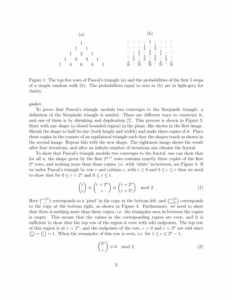
Pascal’s triangle has many interesting properties and one interesting feature comes fromconsidering all numbers modulo two [3]. This ‘binary’ triangle is shown in Figure 2 whereblack and white pixels are used to represent the values modulo two. The figure that appearslooks very much like the Sierpinski triangle (also known as the Sierpinski gasket). Indeed,in the limit of an infinite number of rows, Pascal’s triangle modulo two is the Sierpinski

2

(a)

11 1

1 2 11 3 3 1

1 4 6 4 1

(b)

112

12

14

24

14

18

38

38

18

116

416

616

416

116

0 0 0 0 0 0 0 00 0 0 0 0 00 0 0 00 0

00 0

0 0 00 0 0 0 0

Figure 1: The top five rows of Pascal’s triangle (a) and the probabilities of the first 5 stepsof a simple random walk (b). The probabilities equal to zero in (b) are in light-grey forclarity.

gasket.To prove that Pascal’s triangle modulo two converges to the Sierpinski triangle, a

definition of the Sierpinski triangle is needed. There are different ways to construct it,and one of them is by shrinking and duplication [7]. This process is shown in Figure 3.Start with any shape (a closed bounded region) in the plane, like shown in the first image.Shrink the shape to half its size (both height and width) and make three copies of it. Placethese copies in the corners of an equilateral triangle such that the shapes touch as shown inthe second image. Repeat this with the new shape. The rightmost image shows the resultafter four iterations, and after an infinite number of iterations one obtains the fractal.

To show that Pascal’s triangle modulo two converges to the fractal, one can show thatfor all n, the shape given by the first 2n+1 rows contains exactly three copies of the first2n rows, and nothing more than those copies, i.e. with ‘white’ in-between, see Figure 4. Ifwe index Pascal’s triangle by row r and column c, with r ≥ 0 and 0 ≤ c ≤ r then we needto show that for 0 ≤ r < 2n and 0 ≤ c ≤ r,(

r

c

)≡(r + 2n

c

)≡(r + 2n

c+ 2n

)mod 2. (1)

Here(r+2n

c

)corresponds to a ‘pixel’ in the copy at the bottom left, and

(r+2n

c+2n

)corresponds

to the copy at the bottom right, as shown in Figure 4. Furthermore, we need to showthat there is nothing more than these copies, i.e. the triangular area in-between the copiesis empty. This means that the values in the corresponding region are even, and it issufficient to show that the top row of the region is even with odd endpoints. The top rowof this region is at r = 2n, and the endpoints of the row, c = 0 and c = 2n are odd since(r0

)=(rr

)= 1. When the remainder of this row is even, i.e. for 1 ≤ c ≤ 2n − 1,(

2n

c

)≡ 0 mod 2, (2)

3

mod 2 mod 3

mod 4 mod 5

mod 6 mod 7

Figure 2: The first 180 of rows of Pascal’s triangle shown modulo n where n ∈{2, 3, 4, 5, 6, 7}. If a value was zero modulo n it is coloured white, otherwise it is givena different colour.

4

Figure 3: First few iterations of constructing the Sierpinski triangle. In each iterationthe previous shape is shrunk to half its size and three copies are put in the corners of atriangle so that the shapes are touching.

Pn

Pn+1

row rcolumn c

row r + 2n

columns c , c+ 2n

Figure 4: The first 2n+1 rows of Pascal’s triangle modulo two (Pn+1) contain three copiesof the first 2n rows of the triangle (Pn). A point at row r and column c in the originaltriangle is copied to row r + 2n and columns c and c+ 2n.

5

then the complete region will be even. This is because a value in Pascal’s triangle is thesum of its two neighbours in the row above. Adding two even numbers results in an evennumber, so the next row (r = 2n + 1) will also have even values except near the boundarywhere an even number is added to an odd number. In particular, at every row the size ofthe ‘even part’ in the middle decreases by one, resulting in an empty up-side-down triangleending at r = 2n + 2n − 1 where the two endpoints have joined. By proving that the toprow is even it follows that all entries in the up-side-down triangle are even. We concludethat it is sufficient to prove (1) and (2). For this, one can use Lucas’s theorem.

It is convenient to introduce notation for representing a number by it’s base-p digitsfor a prime p. We will write

n = [nmnm−1 · · ·n0]p =m∑j=0

nj pj with 0 ≤ ni < p for each i,

where the ni are the base-p digits of n

Theorem (Luc1878). Let p be prime and n, k non-negative integers. Let n = [nmnm−1 · · ·n0]pand k = [kmkm−1 · · · k0]p. Then(

n

k

)≡(nmkm

)(nm−1km−1

)· · ·(n0

k0

)mod p, (3)

where we define(nk

)= 0 if k > n.

There are many extensions and generalisations of Lucas’s theorem [9], that includeversions for prime powers or similar congruences for generalised binomial coefficients, butthey are not needed here.

Corollary 1. For any prime p,(n

k

)≡ 0 mod p ⇐⇒ ∃i : ki > ni

Proof. If there is an i such that ki > ni then(ni

ki

)= 0 and by Lucas’s theorem,

(nk

)≡ 0

mod p. Conversely, if ki ≤ ni for all i then(ni

ki

)= ni!

ki!(ni−ki)! . Since ni < p and p is prime,

we have that p is not a factor of ni! and also not a factor of ni!ki!(ni−ki)! . Since p is not a

divisor of(ni

ki

)and p is prime, it also does not divide the product

∏i

(ni

ki

)which concludes

the proof.

The following corollary considers adding extra digits to n and k and is also known asAnton’s Lemma:

Corollary 2. If n, k < pm and then for all l, q ≥ 0,(l · pm + n

q · pm + k

)≡(l

q

)(n

k

)mod p. (4)

6

Proof. When n, k < pm then ni = ki = 0 for i ≥ m, so that l·pm+n = [lM lM−1 · · · l0nm−1nm−2 · · ·n0]pand q · pm + k = [qMqM−1 · · · q0km−1km−2 · · · k0]p. Therefore, by Lucas’s theorem(

l · pm + n

q · pm + k

)≡(lMqM

)(lM−1qM−1

)· · ·(l0q0

)(nm−1km−1

)· · ·(n0

k0

)mod p

≡(l

q

)(n

k

)mod p.

Note that vice versa, Corollary 2 implies Lucas’s theorem by induction on the numberof digits.

We can now prove (1) and (2). By Corollary 2 for p = 2 we have(r + 2n

c

)≡(

1

0

)(r

c

)mod 2,(

r + 2n

c+ 2n

)≡(

1

1

)(r

c

)mod 2,

so (1) follows from(10

)=(11

)= 1. To show (2), note that since 1 ≤ c ≤ 2n − 1 there is a

digit ci that is nonzero for i < n, whereas all digits of r = 2n are zero except for the rn, so(2) follows form Corollary 1.

2.2 Pascals triangle modulo general n

In a similar fashion one can consider Pascal’s triangle modulo general n. Figure 2 showsthis for n ∈ {2, 3, 4, 5, 6, 7}. We can distinguish cases for primes, prime powers and othernumbers.

2.2.1 Pascals triangle modulo a prime

When n is a prime (2,3,5,7 in the figure), one obtains a generalisation of Sierpinski’striangle. This generalisation for primes p can also be constructed using the shrinkingand duplication method. When using the shrinking and duplication construction, one canstart with an arbitrary shape, shrink it and create p(p + 1)/2 copies. These copies haveto be arranged into a larger triangle where all the copies are touching. The proof is ageneralisation of the one given in the previous section. One has to show that(

r

c

)≡(r + l · pn

c+ q · pn

)mod p,

where 0 ≤ l < p and 0 ≤ q ≤ l. Each value of (l, q) corresponds to one of the p(p + 1)/2copies. This equivalence follows from Corollary 2 and

(lq

)6≡ 0 mod p. The empty up-

side-down triangles correspond to(r+l·pmc+q·pm

)but where the range of c is now r < c < pm as

7

mod 3 mod 32

mod 33

mod 34

Figure 5: Pascal’s triangle plotted modulo powers of 3. The colours give the 3-adicvaluation ν3(

(rc

)), where black is 0, orange is 1, red is 2 and blue is 3.

opposed to 0 ≤ c ≤ r. This case is also included in Corollary 2, and as(rc

)= 0 for r < c

this finishes the proof.

2.2.2 Pascals triangle modulo a composite number

When n is composite (mod 6 in the figure) then the resulting shape is the union of theshapes obtained of its factors (prime powers) albeit with different colours. For example,at n = 6, shown in Figure 2 one can see the union of the shapes of p = 2 and p = 3. Thisis simply because when n = pk11 · · · pkmm then x ≡ 0 mod n if and only if for all i : x ≡ 0mod pkii .

2.2.3 Pascals triangle modulo a prime power

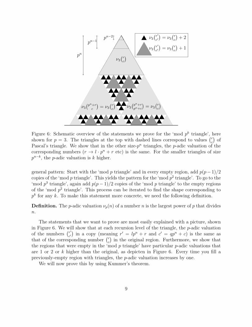
When n is a prime power then the pattern becomes slightly more complicated. One can seein Figure 2 that for n = 4, the image is the same as for n = 2 but with extra triangles in theplaces that used to be empty. When one would consider n = 8, this idea is repeated and theholes in the n = 4 shape are filled with additional triangles. Figure 5 shows what happenswhen the triangle is plotted modulo powers of 3. From the Figure we can conjecture the

8

ν3(rc

)

ν3(pn+rc

)= ν3

(rc

)ν3(pn+rpn+c

)= ν3

(rc

)

ν3(r′

c′

)= ν3

(rc

)+ 2

ν3(r′

c′

)= ν3

(rc

)+ 1

pn

pn−1pn−2

Figure 6: Schematic overview of the statements we prove for the ‘mod pk triangle’, hereshown for p = 3. The triangles at the top with dashed lines correspond to values

(rc

)of

Pascal’s triangle. We show that in the other size-pn triangles, the p-adic valuation of thecorresponding numbers (r → l · pn + r etc) is the same. For the smaller triangles of sizepn−k, the p-adic valuation is k higher.

general pattern: Start with the ‘mod p triangle’ and in every empty region, add p(p− 1)/2copies of the ‘mod p triangle’. This yields the pattern for the ‘mod p2 triangle’. To go to the‘mod p3 triangle’, again add p(p− 1)/2 copies of the ‘mod p triangle’ to the empty regionsof the ‘mod p2 triangle’. This process can be iterated to find the shape corresponding topk for any k. To make this statement more concrete, we need the following definition.

Definition. The p-adic valuation νp(n) of a number n is the largest power of p that dividesn.

The statements that we want to prove are most easily explained with a picture, shownin Figure 6. We will show that at each recursion level of the triangle, the p-adic valuationof the numbers

(r′

c′

)in a copy (meaning r′ = lpn + r and c′ = qpn + c) is the same as

that of the corresponding number(rc

)in the original region. Furthermore, we show that

the regions that were empty in the ‘mod p triangle’ have particular p-adic valuations thatare 1 or 2 or k higher than the original, as depicten in Figure 6. Every time you fill apreviously-empty region with triangles, the p-adic valuation increases by one.

We will now prove this by using Kummer’s theorem.

9

Theorem (Kum1852). Let p be prime and n, k non-negative integers, n ≥ k. Then thep-adic valuation νp(

(nk

)) of

(nk

)is equal to the number of “carries” when k and n − k are

added in base-p arithmetic.

One way to find the number of carries that occur when k is added to n − k in base-pis by considering the base-p digits of n and k, defining cn,k−1 = 0 and

cn,ki =

1 ni < ki

0 ni > ki

cn,ki−1 ni = ki

.

The number of carries is then equal to∑

i≥0 cn,ki . Kummer’s theorem can therefore be

written as νp((nk

)) =

∑i≥0 c

n,ki .

The following claim shows what happens to νp((nk

)) when a digit l is added to n and a

digit q is added to k:

Claim 1. Let p be prime and n, k, q, l,m non-negative integers with 0 ≤ k ≤ n < pm and0 ≤ q ≤ l < p. Then

νp(

(l · pm + n

q · pm + k

)) = νp(

(n

k

))

Proof. Define n′ = l · pm + n and k′ = q · pm + k. Note that n, k have at most m − 1digits when expressed in base p and l, q are the m-th digits of n′ and k′. Note that we havecn,ki = cn

′,k′

i for i < m since the first m−1 digits are the same. For the m-th digits we have

cn′,k′

m =

1 l < q

0 l > q

cn,km−1 l = q

.

By Kummer’s theorem the difference between νp((n′

k′

)) and νp(

(nk

)) is equal to cn

′,k′m , so it

remains to show that cn′,k′m = 0. By assumption we know q ≤ l and if q < l we have

cn′,k′m = 0 by definition. Consider the case l = q where we have cn

′,k′m = cn,km−1. If n = k then

all the cn,ki are zero so we are done. If n 6= k then the consider the most significant digitwhere n and k differ, i.e. take the highest i for which ni 6= ki and call it i∗. Since k < n byassumption, it must be true that ki∗ < ni∗ and therefore cn,ki∗ = 0. For all i > i∗ we haveni = ki so cn,ki = cn,ki−1. So cn

′,k′m = cn,ki∗ = 0.

Claim 2. If νp(n) = νp(m) then for any k

n ≡ 0 mod pk ⇐⇒ m ≡ 0 mod pk.

10

Proof. It follows from the fact that n ≡ 0 mod pk if and only if νp(n) ≥ k.

Consider Figure 5. The size of the recursion levels in the ‘mod pk triangle’ is the sameas in the mod p triangle, meaning powers of p and not powers of pk. Repeating what wedid before for the mod p triangle, we can see that at recursion level n, the “copies” and“empty regions” correspond to the following binomial coefficients of Pascal’s triangle:(

l · pn + r

q · pn + c

)“copies”→ 0 ≤ q ≤ l < p , 0 ≤ c ≤ r < pn

“empty”→ 0 ≤ q < l < p , 0 ≤ r < c < pn.

Here n is the recursion level and (l, q) index the different copies or empty regions whereasr and c index points within those regions. By claim 1, the p-adic valuation of a number(r′

c′

)in the copy is the same as that of the corresponding original number

(rc

). By Claim 2,

we have now shown that for any k, the copies in the ‘mod pk triangle’ are indeed all thesame.

What is left to show is how the empty regions of the ‘mod p triangle’ are filled. We willfirst consider k = 2. The new triangles in the mod p2 shape can be indexed as follows:(

l · pn + s · pn−1 + r

q · pn + t · pn−1 + c

)with

0 ≤ q < l < p ,0 ≤ s < t < p ,0 ≤ c ≤ r < pn−1.

These lie within the empty regions of the mod p triangle. Similar to the proof of Claim 1we can let the carries cr

′,c′

i be defined as before, for the numbers r′ = [l s rn−2rn−3...r0]pand c′ = [q t cn−2...c0]p. We have q < l hence cr

′,c′n = 0 and s < t so cr

′,c′

n−1 = 1. This meansthere is exactly one extra carry compared to r and c and hence by Kummer’s theorem

νp(

(l · pn + s · pn−1 + r

q · pn + t · pn−1 + c

)) = νp(

(r

c

)) + 1

for these values of l, q, s, t, r, c. This is what we need, because it implies(l · pn + s · pn−1 + r

q · pn + t · pn−1 + c

)≡ 0 mod pk+1 ⇐⇒

(r

c

)≡ 0 mod pk

i.e. in the mod pk+1 shape there is a copy of the (smaller) mod pk shape. This proves whatwas drawn as a size-pn triangle in Figure 6. If we continue to the triangles that are newlyadded in the ‘mod 33 triangle’, we find that they correspond to(

r′n · pn + r′n−1 · pn−1 + r′n−2 · pn−2 + r

c′n · pn + c′n−1 · pn−1 + c′n−2 · pn−2 + c

)

with

0 ≤ c′n < r′n < p ,0 ≤ r′n−1 ≤ c′n−1 < p ,0 ≤ r′n−2 < c′n−2 < p ,0 ≤ c ≤ r < pn−2.

11

Define r′ = [r′nr′n−1r

′n−2rn−3 · · · r0]p and c′ = [c′nc

′n−1c

′n−2cn−3 · · · c0]p. Then by the same

reasoning as before we can apply Kummer’s theorem to obtain νp((r′

c′

)) = νp(

(rc

)) + cr

′,c′

n−2 +

cr′,c′

n−1 + cr′,c′n . Looking at the constraints for digits n− 2 up to n we see that cr

′,c′n = 0, and

cr′,c′

n−1 is 1 or equal to cr′,c′

n−2 which is always 1. We conclude: ν3((r′

c′

)) = ν3(

(rc

)) + 2. We

can continue the pattern, and we find that in the ‘mod pk+1 triangle’, the newly addedtriangles correspond to the following constraints on the digits of r′, c′ with the followingcarries:

0 ≤ c′n < r′n < p cr′,c′

n = 0

0 ≤ r′n−1 ≤ c′n−1 < p cr′,c′

n−1 = 1 or cr′,c′

n−1 = cr′,c′

n−2...

0 ≤ r′n−k+1 ≤ c′n−k+1 < p cr′,c′

n−k+1 = 1 or cr′,c′

n−k+1 = cr′,c′

n−k

0 ≤ r′n−k < c′n−k < p cr′,c′

n−k = 1

0 ≤ c ≤ r < pn−k ν3

(r

c

).

We see that ν3(r′

c′

)= ν3

(rc

)+k as required. We still have to show that the empty regions in

the ‘mod pk+1 triangle’ are empty. They correspond to the same indices as above exceptfor 0 ≤ r′n−k ≤ c′n−k < p and 0 ≤ r < c < pn−k. We can apply the same idea as in theproof of Claim 1 by noting that the first digit where r and c differ will satisfy ri∗ < ci∗ andhence all the carries cr

′,c′

i are 1 for i ≥ i∗. This gives ν3(r′

c′

)≥ k + 1, meaning that

(r′

c′

)≡ 0

mod pk+1 so the region is indeed empty.

Since the numbers in Pascal’s triangle can be thought of as scaled probabilities of arandom walk, one could imagine writing down probabilities of a quantum walk, scaled tobecome integer, and show them modulo two. The next section will introduce a specificquantum walk and apply this idea with p = 2 and p = 3.

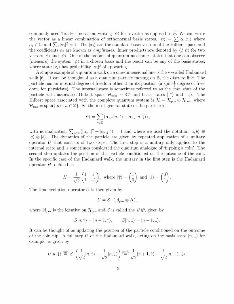
3 Hadamard Walk

Quantum walks are simple models for a quantum particle moving through some system.This paper is only concerned with the probability distribution that emerges from oneparticular quantum walk, and therefore the physical aspects of it are left out. Here weonly provide a short overview of the relevant concepts, and we refer the reader to [8] fora complete introduction to the field of quantum information. For the purposes of thispaper we only need to know that the state of a particle is described by a unit vector ina complex Hilbert space, and quantum mechanics dictates that time evolution is limitedto applying unitary operators to this vector. We will denote such state vectors using the

12

commonly used ‘bra-ket’ notation, writing |ψ〉 for a vector as opposed to ~ψ. We can writethe vector as a linear combination of orthonormal basis states, |ψ〉 =

∑i αi|xi〉 where

αi ∈ C and∑

i |αi|2 = 1. The |xi〉 are the standard basis vectors of the Hilbert space andthe coefficients αi are known as amplitudes. Inner products are denoted by 〈φ|ψ〉 for twovectors |φ〉 and |ψ〉. One of the axioms of quantum mechanics states that one can observe(measure) the system |ψ〉 in a chosen basis and the result can be any of the basis states,where state |xi〉 has probability |αi|2 of appearing.

A simple example of a quantum walk on a one-dimensional line is the so-called Hadamardwalk [6]. It can be thought of as a quantum particle moving on Z, the discrete line. Theparticle has an internal degree of freedom other than its position (a spin-1

2degree of free-

dom, for physicists). The internal state is sometimes referred to as the coin state of theparticle with associated Hilbert space Hcoin = C2 and basis states | ↑〉 and | ↓〉. TheHilbert space associated with the complete quantum system is H = Hpos ⊗ Hcoin whereHpos = span{|n〉 | n ∈ Z}. So the most general state of the particle is

|ψ〉 =∑n∈Z

(αn,↑|n, ↑〉+ αn,↓|n, ↓〉) ,

with normalization∑

n∈Z (|αn,↑|2 + |αn,↓|2) = 1 and where we used the notation |a, b〉 ≡|a〉 ⊗ |b〉. The dynamics of the particle are given by repeated application of a unitaryoperator U that consists of two steps. The first step is a unitary only applied to theinternal state and is sometimes considered the quantum analogue of ‘flipping a coin’. Thesecond step updates the position of the particle conditioned on the outcome of the coin.In the specific case of the Hadamard walk, the unitary in the first step is the Hadamardoperator H, defined as

H =1√2

(1 11 −1

), where |↑〉 =

(10

)and |↓〉 =

(01

).

The time evolution operator U is then given by

U = S · (Idpos ⊗H),

where Idpos is the identity on Hpos and S is called the shift, given by

S|n, ↑〉 = |n+ 1, ↑〉, S|n, ↓〉 = |n− 1, ↓〉.

It can be thought of as updating the position of the particle conditioned on the outcomeof the coin flip. A full step U of the Hadamard walk, acting on the basis state |n, ↓〉 forexample, is given by

U |n, ↓〉 coin= S

(1√2|n, ↑〉 − 1√

2|n, ↓〉

)shift=

1√2|n+ 1, ↑〉 − 1√

2|n− 1, ↓〉.

13

1√2

1√2

1√2

−1√2

|−3〉p|−2〉p|−1〉p |0〉p |1〉p |2〉p |3〉p

|↑〉c

|↓〉c

Figure 7: Graphical representation of one step U of the Hadamard walk. The dots representpossible quantum states of the form |n, ↑〉 (top row) and |n, ↓〉 (bottom row) and the arrowsrepresent one application of the coin and shift when starting at position 0. The arrow goingfrom |0, ↓〉 to |−1, ↓〉 represents that the amplitude at |0, ↓〉 is multiplied by −1/

√2 and

then stored at |−1, ↓〉, added to a part of the amplitude coming from |0, ↑〉.

If we now were to measure the system, the result would be either |n + 1, ↑〉 or |n − 1, ↓〉,both with probability |±1/

√2|2 = 1/2. Figure 7 shows a schematic representation of one

step U of the Hadamard walk.With these definitions, one can now consider the following process. Select a starting

state, say |ψs〉 = |0, ↑〉, evolve it with U for t steps and then measure the position. Forexample, starting in |0, ↑〉, the state of the system after three steps is given by

U3|0, ↑〉 =1

(√

2)3

(|−3, ↓〉 − |−1, ↑〉+ 2|1, ↑〉+ |1, ↓〉+ |3, ↑〉

).

Now measuring the system will result in finding some positionX with probabilities P[X=−3] =18, P[X=−1] = 1

8, P[X=1] = 5

8and P[X=3] = 1

8. The amplitudes of the first five steps are

also displayed in Figure 8.

3.1 Hadamard triangle

The numbers in Pascal’s triangle can be thought of as scaled probabilities of a random walk,and carrying this idea over to the Hadamard walk, one could consider the amplitudes orprobabilities of the Hadamard walk, but scaled by a factor of

√2n so that all numbers

involved become integer. Another way to view this is instead of applying H, use√

2H, amatrix with only integer coefficients. Note that we could either use the amplitudes or theprobabilities which are simply their squares. However, since we are primarily interested inwhether or not they are divisible by some prime p, squaring the amplitudes does not makea difference. We therefore continue with the (unsquared) amplitudes. Figure 8 shows thestart of the Hadamard triangle. We will now derive expressions for these amplitudes whenstarting in |0, ↑〉.

14

1√20

1√21

1√22

1√23

1√24

(1 , 0)

(0 , 1) (1 , 0)

(0 , −1) (1 , 1) (1 , 0)

(0 , 1) (−1 , 0) (2 , 1) (1 , 0)

(0 , −1) (1 , −1) (−1 , 1) (3 , 1) (1 , 0)

Figure 8: The up- and down-components of the amplitudes of the first 5 steps of theHadamard walk, starting in |0, ↑〉. Every row corresponds to one time-step. The normali-sation of each row is shown at the left side. At even timesteps, only the even positions areshown and at odd time-steps only the odd positions are shown, similar to Figure 1. Thearrows represent the time-step of the Hadamard walk. A dotted arrow means the incomingamplitude is multiplied by −1 before being added to the other incoming amplitude. Thered and blue colouring denotes a subset of amplitudes that is used in Section 3.3 and 3.4.

3.2 Expressions for amplitudes

Meyer [5] gave explicit expressions for the amplitudes encountered in the Hadamard walk.Let ψ↑(n, t) be the amplitude at |n, ↑〉 after t steps when starting in |0, ↑〉, i.e. ψ↑(n, t) :=〈n, ↑|U t|0, ↑〉. Similarly, let ψ↓(n, t) := 〈n, ↓|U t|0, ↑〉. Then we have

Lemma ([5]). When t+n is odd or when |n| > t we have ψ↑(n, t) = ψ↓(n, t) = 0. Otherwisethe amplitudes are given by

ψ↑(n, t) =

{1√2t

n = t1√2t

∑k≥1((t−n)/2−1

k−1

)((t+n)/2

k

)(−1)(t−n)/2−k n < t

ψ↓(n, t) =1√2t

∑k≥0

((t− n)/2− 1

k

)((t+ n)/2

k

)(−1)(t−n)/2−k−1

We will give an alternative and slightly shorter proof of this for a general coin operator.This proof also allows us to make another observation stated in the following claim. LetC be any unitary 2x2 matrix. Any such matrix can be written as follows

C =

(cr cucd cl

)=

( √p eiα

√1− p eiβ

−√

1− p eiγ √p ei(γ+β−α))

, with 0 ≤ p ≤ 1.

15

cr

cd cu

cl

cr

cd cu

cl

cr

cd cu

cl

cr

cd cu

cl

cr

cd cu

cl

−3

−3

−2

−2

−1

−1

0

0

1

1

2

2

3

3

|↑〉

|↓〉

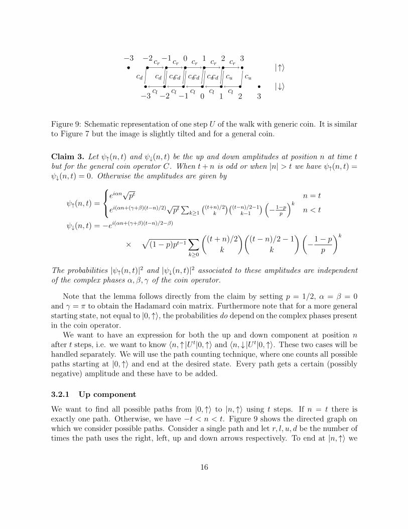
Figure 9: Schematic representation of one step U of the walk with generic coin. It is similarto Figure 7 but the image is slightly tilted and for a general coin.

Claim 3. Let ψ↑(n, t) and ψ↓(n, t) be the up and down amplitudes at position n at time tbut for the general coin operator C. When t+ n is odd or when |n| > t we have ψ↑(n, t) =ψ↓(n, t) = 0. Otherwise the amplitudes are given by

ψ↑(n, t) =

eiαn√pt n = t

ei(αn+(γ+β)(t−n)/2)√pt∑

k≥1((t+n)/2

k

)((t−n)/2−1

k−1

) (−1−p

p

)kn < t

ψ↓(n, t) = −ei(αn+(γ+β)(t−n)/2−β)

×√

(1− p)pt−1∑k≥0

((t+ n)/2

k

)((t− n)/2− 1

k

)(−1− p

p

)kThe probabilities |ψ↑(n, t)|2 and |ψ↓(n, t)|2 associated to these amplitudes are independentof the complex phases α, β, γ of the coin operator.

Note that the lemma follows directly from the claim by setting p = 1/2, α = β = 0and γ = π to obtain the Hadamard coin matrix. Furthermore note that for a more generalstarting state, not equal to |0, ↑〉, the probabilities do depend on the complex phases presentin the coin operator.

We want to have an expression for both the up and down component at position nafter t steps, i.e. we want to know 〈n, ↑|U t|0, ↑〉 and 〈n, ↓|U t|0, ↑〉. These two cases will behandled separately. We will use the path counting technique, where one counts all possiblepaths starting at |0, ↑〉 and end at the desired state. Every path gets a certain (possiblynegative) amplitude and these have to be added.

3.2.1 Up component

We want to find all possible paths from |0, ↑〉 to |n, ↑〉 using t steps. If n = t there isexactly one path. Otherwise, we have −t < n < t. Figure 9 shows the directed graph onwhich we consider possible paths. Consider a single path and let r, l, u, d be the number oftimes the path uses the right, left, up and down arrows respectively. To end at |n, ↑〉 we

16

then have

r + l + u+ d = t total number of steps

r − l = n ending column

u = d start up and end up

Let k = u = d, then we have r = t+n2− k and l = t−n

2− k. We have k ≥ 1 (we need to go

down and up at least once) and k ≤ t−n2, t+n

2.

For a specific set of values (r, l, u, d) the path will arrive with an amplitude (cr)r(cl)

l(cu)u(cd)

d.So we sum over all possible values for (r, l, u, d) and count how many paths there are fora specific set of values (r, l, u, d). We can construct such paths as follows. Construct a se-quence of choices to make if the walker is in the top layer and another sequence of choicesto make if the walker is in the bottom layer. The walker is in the | ↑〉 state (top layer)k + r = t+n

2times, out of which r times it goes right and k times it goes down. There are(

(t+n)/2k

)possible ways to do this. Likewise, the particle is in |↓〉 (bottom layer) l+k = t−n

2

times and has to choose between left and up. The last of these choices should always beup, so this gives

((t−n)/2−1

k−1

)possibilities. To construct the full path, start with the top-layer

choices, and whenever the choice is ‘down’, continue with the bottom-layer choices and soon. Therefore

〈n, ↑ |U t|0, ↑〉 =

{(cr)

t n = t∑k≥1((t+n)/2

k

)((t−n)/2−1

k−1

)c(t+n)/2−kr c

(t−n)/2−kl ckuc

kd n < t

.

Now rewrite the last sum for n < t and group the factors that do not depend on k:

c(t+n)/2r c(t−n)/2l

∑k≥1

((t+ n)/2

k

)((t− n)/2− 1

k − 1

)(cucdcrcl

)kNote that cucd

crcl= −1−p

pso this fraction is always a real (negative) number, regardless of

the complex phases present in the entries of the coin matrix. The sum above in terms ofp and α, β, γ is equal to

ei(αn+(γ+β)(t−n)/2)√pt∑k≥1

((t+ n)/2

k

)((t− n)/2− 1

k − 1

)(−1− p

p

)k,

as claimed. The probability |ψ↑(n, t)|2 of being at |n, ↑〉 after t steps when starting in |0, ↑〉is independent of α, β, γ since the only dependence on these variables is in the prefactorei(αn+(γ+β)(t−n)/2) which always has norm 1.

17

3.2.2 Down component

For the down component, the equations are similar:

r + l + u+ d = t total number of steps

r − l = n+ 1 ending column (tilted)

u+ 1 = d start up and end down

Let u = k, then the equations give r = (t+n)/2−k and l = (t−n)/2−k−1. The argumentis the same as before, but now the last choice in the top layer has to be ‘down’ with norestrictions on the last choice in the bottom layer. We are in |↑〉 r+d = (t+n)/2+1 times.The last choice has to be down, so this gives

((t+n)/2

k

). We are in |↓〉 l + u = (t− n)/2− 1

times which gives((t−n)/2−1

k

). The expression is therefore given by

ψ↓(n, t) =∑k≥0

((t+ n)/2

k

)((t− n)/2− 1

k

)ckuc

k+1d c

(t−n)/2−k−1l c(t+n)/2−kr .

Rewriting this in terms of p, α, β, γ gives the expression given in the claim. Again the onlydependency on the complex phases is in the prefactor which has norm 1 so the probability|ψ↓(n, t)|2 only depends on p.

3.3 Hadamard walk modulo 2 - Sierpinski triangle

When the amplitudes of the Hadamard walk are plotted modulo two, the Sierpinski triangleappears in a similar fashion to Pascal’s triangle. To see why this is the case, we note thatto find the amplitudes at some time t modulo two it is enough to consider a process whereevery single time-step is done modulo two. The scaled Hadamard operator becomes

√2H ≡

(1 11 1

)mod 2,

and we can immediately see that the amplitude sent to the right is the same as the am-plitude sent to the left. More precisely, after any time-step the amplitude at |n − 1, ↓〉 isthe same as the amplitude at |n+ 1, ↑〉 modulo two, for all n. This idea is shown in Figure10 which is similar to Figure 8 but modulo two. An ellipse is drawn around the pairs ofamplitudes of states |n− 1, ↓〉 and |n+ 1, ↑〉. The figure shows that the two values in eachellipse are equal, and are the sum of the values in the two neighbouring ellipses above it.This is the same rule with which Pascal’s triangle can be constructed. Indeed, taking onevalue out of every ellipse, the Sierpinski triangle can be obtained. These are the either thered or the blue values shown in Figure 8.

18

(1 , 0)

(0 , 1) (1 , 0)

(0 , 1) (1 , 1) (1 , 0)

(0 , 1) (1 , 0) (0 , 1) (1 , 0)

(0 , 1) (1 , 1) (1 , 1) (1 , 1) (1 , 0)

Figure 10: Amplitudes of the first 5 steps of the scaled Hadamard walk modulo two,starting in |0, ↑〉. It is similar to Figure 8 but the amplitudes are considered modulo two.Every pair (·, ·) corresponds to up and down components of the state. The dotted arrow inFigure 8 becomes a normal arrow because −1 ≡ 1 mod 2. The red ellipses indicate pairsof values that are the same and form Pascal’s triangle modulo two.

xy

position n

time t

3n+1

3n

l =0

l =1

l =2

q=0

q=1

q=2

Figure 11: The start of the Sierpinski carpet resulting from colouring the scaled Hadamardwalk amplitudes modulo 3. The horizontal direction is position and the vertical directionis time. The shape drawn at each point is a diamond, i.e. a rotated square instead of asquare, because this gives a better visualisation of the x, y coordinates.

19

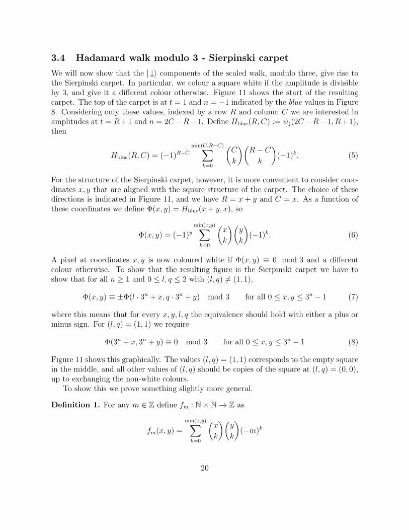
3.4 Hadamard walk modulo 3 - Sierpinski carpet

We will now show that the | ↓〉 components of the scaled walk, modulo three, give rise tothe Sierpinski carpet. In particular, we colour a square white if the amplitude is divisibleby 3, and give it a different colour otherwise. Figure 11 shows the start of the resultingcarpet. The top of the carpet is at t = 1 and n = −1 indicated by the blue values in Figure8. Considering only these values, indexed by a row R and column C we are interested inamplitudes at t = R+ 1 and n = 2C−R−1. Define Hblue(R,C) := ψ↓(2C−R−1, R+ 1),then

Hblue(R,C) = (−1)R−Cmin(C,R−C)∑

k=0

(C

k

)(R− Ck

)(−1)k. (5)

For the structure of the Sierpinski carpet, however, it is more convenient to consider coor-dinates x, y that are aligned with the square structure of the carpet. The choice of thesedirections is indicated in Figure 11, and we have R = x + y and C = x. As a function ofthese coordinates we define Φ(x, y) = Hblue(x+ y, x), so

Φ(x, y) = (−1)ymin(x,y)∑k=0

(x

k

)(y

k

)(−1)k. (6)

A pixel at coordinates x, y is now coloured white if Φ(x, y) ≡ 0 mod 3 and a differentcolour otherwise. To show that the resulting figure is the Sierpinski carpet we have toshow that for all n ≥ 1 and 0 ≤ l, q ≤ 2 with (l, q) 6= (1, 1),

Φ(x, y) ≡ ±Φ(l · 3n + x, q · 3n + y) mod 3 for all 0 ≤ x, y ≤ 3n − 1 (7)

where this means that for every x, y, l, q the equivalence should hold with either a plus orminus sign. For (l, q) = (1, 1) we require

Φ(3n + x, 3n + y) ≡ 0 mod 3 for all 0 ≤ x, y ≤ 3n − 1 (8)

Figure 11 shows this graphically. The values (l, q) = (1, 1) corresponds to the empty squarein the middle, and all other values of (l, q) should be copies of the square at (l, q) = (0, 0),up to exchanging the non-white colours.

To show this we prove something slightly more general.

Definition 1. For any m ∈ Z define fm : N× N→ Z as

fm(x, y) =

min(x,y)∑k=0

(x

k

)(y

k

)(−m)k

20

The reason for the minus sign in (−m)k is that all valid quantum walks will have m ≥ 0this way, as will become clear later. As a side note, this function is a special case of the so-called hypergeometric function 2F1(a, b; c; z), namely fm(x, y) = 2F1(−x,−y, 1,−m). Thefollowing claim could be seen as something similar to Corollary 2 but for fm:

Claim 4. Let p be a prime and let 0 ≤ l, q ≤ p− 1. Then we have for all m ∈ Z and forall 0 ≤ x, y ≤ pn − 1

fm(l · pn + x , q · pn + y) ≡ fm(l, q) · fm(x, y) mod p.

Proof. Note that any sum can be split in the following way:

pn+1−1∑k=0

g(k) =

p−1∑s=0

pn−1∑k=0

g(s · pn + k),

where s takes the role of the most significant digit and k takes the role of the other digits.We apply this idea to the sum in fm(x, y) where we note that min(lpn+x, qpn+y) ≤ pn+1−1but we can let the sum range all the way to pn+1 − 1 because the summand is zero in thisextra range. Therefore we have

fm(l · pn + x , q · pn + y) =

pn+1−1∑k=0

(l · pn + x

k

)(q · pn + y

k

)(−m)k

=

p−1∑s=0

pn−1∑k=0

(l · pn + x

s · pn + k

)(q · pn + y

s · pn + k

)(−m)s·p

n+k

Note that by Fermat’s little theorem we have mp ≡ m mod p so ms·pn ≡ ms mod p. Nowwe apply Corollary 2 to the binomial coefficients to obtain

fm(l · pn + x , q · pn + y) ≡p−1∑s=0

pn−1∑k=0

(l

s

)(q

s

)(x

k

)(y

k

)(−m)s+k

≡

(p−1∑s=0

(l

s

)(q

s

)(−m)s

)fm(x, y)

≡ fm(l, q) · fm(x, y) mod p,

as required.

Note that l, q take the role of the most significant digits and x, y are the other digits.Just as Corollary 2 implies Lucas’s theorem, we can apply this claim inductively on thenumber of digits to arrive at a result very similar to Lucas’s theorem but now for thefunction fm:

21

Lemma 1 (Lucas’-like theorem for fm). Let p be prime and x, y non-negative integers.Let x = [xnxn−1 · · ·x0]p and y = [ynyn−1 · · · y0]p. Then for all m ∈ Z we have

fm(x, y) ≡ fm(xn, yn) fm(xn−1, yn−1) · · · fm(x0, y0) mod p.

We can now prove (7) and (8) by noting that Φ(x, y) = (−1)yf1(x, y) so by Claim 4 wehave

Φ(l · 3n + x, q · 3n + y) ≡ (−1)q·3n

f1(l, q)Φ(x, y) ≡ Φ(l, q)Φ(x, y) mod 3.

where we used that (−1)q·3n

= (−1)q. Note that Φ(1, 1) = 0 which proves (8) and Φ(l, q) ≡±1 mod 3 for the other values of l, q which proves (7).

3.5 Results for a more general quantum walk

We can generalize the results of the previous section. First of all, we can consider the samenumbers modulo any prime p. But more generally, the Hadamard operator H could bereplaced by any matrix C ∈ U(2). As stated before, we can write any unitary 2× 2 matrixas

C =

(cr cucd cl

)=

( √p eiα

√1− p eiβ

−√

1− p eiγ √p ei(γ+β−α))

, with 0 ≤ p ≤ 1.

The expression for the amplitudes with general coin operator is given by ψ↓(n, t) as givenin Claim 3, and we can do the same substitutions as before to go to the x, y coordinates:

ΦC(x, y) = cdcxrcyl

∑k≥0

(x

k

)(y

k

)(−1− p

p

)k= cdc

xrcyl fm(x, y).

where m = (1 − p)/p and we extend the definition of fm for non-integer m. Note that(1 − p)/p ≥ 0 for any valid coin which was the reason for defining fm with a minus sign.In the previous sections we considered the amplitudes of the quantum walk as opposedto the probabilities (which are equal to the norm squared of the amplitudes). For thepurpose of the Sierpinski carpet, this distinction was not important because all entries ofthe Hadamard matrix are real and we were only interested in whether or not an integerwas zero modulo a prime. Since x ≡ 0 mod p ⇐⇒ x2 ≡ 0 mod p, squaring did notmatter. For a general coin, however, there could be complex amplitudes and so we considerthe corresponding probabilities to make sure all numbers involved are real. Note that sincefm is real, the imaginary component of ΦC(x, y) comes only from cdc

xrcyl . We therefore

consider the probabilities:

|ΦC(x, y)|2 = |cdcxrcyl |

2 (fm(x, y))2 .

22

In the previous sections we rescaled the Hadamard matrix by a factor of√

2 so that allnumbers involved became integer. For a general coin matrix, in order to consider theprobabilities modulo a prime, we assume that the coin matrix is such that m = (1 −p)/p is integer. Note that this can not be achieved by scaling the entire matrix becausem is invariant under such scalings. In fact, we have p = 1

1+mand m ≥ 0 has to be

integer. Furthermore, as stated in Claim 4, the complex phases α, β, γ do not influence|ΦC(x, y)|2. Therefore the most general form of the matrix we can consider to obtaininteger probabilities is the unitary matrix

Cm =

(√1/(1 +m)

√m/(1 +m)√

m/(1 +m) −√

1/(1 +m)

)for m ∈ Z, m ≥ 0,

where have set α = β = 0 and γ = π such that C1 = H, but any other setting of phaseswould be equally valid. If we want to scale the matrix by a factor λ such that |cdcxrc

yl |2 is

integer then this requires λ =√n(1 +m) for any integer n ≥ 1. This gives a scaled matrix√

n(1 +m)Cm =√n

(1√m√

m −1

), (9)

and for this scaled matrix, |cdcxrcyl |2 = mnx+y+1. By Claim 4 we have for this scaled coin

matrix that

|ΦC(l · pn + x, q · pn + y)|2 ≡ n(l+q)(pn−1)−1

m|ΦC(l, q)|2 |ΦC(x, y)|2 mod p

≡ 1

mn|ΦC(l, q)|2 |ΦC(x, y)|2 mod p,

where we used Fermat’s little theorem in the second step. For m = 1 and n = 1 we recoverthe exact same rules as for the Hadamard matrix. This class also includes the commonlyused coin

1√2

(1 ii 1

).

To find out what kind of fractals are generated by these quantum walks, it is useful tonote that we are only interested in distinguishing |Φ(x, y)|2 ≡ 0 mod p from |Φ(x, y)|2 6≡ 0mod p. Since we have |Φ(x, y)|2 = mnx+y+1(fm(x, y))2 we can see that if m ≡ 0 mod por n ≡ 0 mod p then all values |Φ(x, y)|2 are zero modulo p and there is no fractal sinceall pixels are white. Therefore, assume that both m and n are not zero modulo p. In thatcase we have |Φ(x, y)|2 ≡ 0 mod p if and only if fm(x, y) ≡ 0 mod p. Now we can applythe quantum version of Lucas’ theorem. By Lemma 1, fm(x, y) ≡ 0 mod p if and only ifthere is an i such that fm(xi, yi) ≡ 0 mod p, where xi, yi are the base-p digits of x, y.

In general, to find the fractal generated by a quantum walk with the general coin fromEquation (9) for some n,m that are non-zero modulo p, we simply have to compute fm(x, y)

23

mod p for only 0 ≤ x, y < p to find what we call the base image. Figure 12 shows thesebase images for several values of m and p. From this the fractal can be constructed in asimple recursive way, shown in Figure 13, resulting in the fractals shown in Figure 14. Thisrecursive method is valid because each recursion step corresponds to adding another digitto x and y, and as mentioned above, a pixel will be white if and only if there are digits(i.e. a recursion step) in which the region corresponding to those digits is white. In case ofthe example construction (Figure 13), the third picture corresponds to x, y values in therange 0 ≤ x, y < 23 which can be described by three digits modulo 2. Let x = [x2x1x0]2and y = [y2y1y0]2, then x2, y2 specify which of the four biggest quadrants the pixel is in.Likewise, x1, y1 specify which of the four subquadrants of that first quadrant it is in, andx0, y0 specify the final position within that subquadrant. By the construction in Figure13, the pixel will be white if and only if one of those chosen quadrants was bottom-right.This is equivalent to saying that the pixel is white if and only if there is an i such thatfm(xi, yi) ≡ 0 mod p.

3.6 Other properties of the Hadamard triangle

One can add the probabilities in each row of the triangle and by unitarity this sum willalways be equal to one. Instead one can also consider summing all the amplitudes in arow. Define the column vector Ψ(t) = (Ψ↑(t) Ψ↓(t))

T where Ψ↑(t) is the sum of the upamplitudes at time t, i.e.

Ψ↑(t) =t∑

n=−t

ψ↑(n, t),

and similar for Ψ↓(t). Alternatively, consider the linear map

Σ =∑n∈Z

〈n|,

so that Ψ(t) = Σ U t|0, ↑〉. Note that to go from time t to t + 1, one application of acoin and shift is performed (U = S(Id ⊗H)), but the sums of all up or down amplitudesare invariant under the shift operation. In other words ΣS = Σ. Furthermore we haveΣ(Id⊗H) = HΣ, so we have

ΣU t = Σ(S(Id⊗H))t = H tΣ.

This can also be seen by simply looking at Figure 8, and noting that Ψ↑(t+1) = 1√2(Ψ↑(t)+

Ψ↓(t)) and Ψ↓(t+ 1) = 1√2(Ψ↑(t)−Ψ↓(t)), or simply

Ψ(t+ 1) = HΨ(t).

24

mod 2 mod 3 mod 5 mod 7 mod 11 mod 13 mod 17

m = 1

m = 2 m ≡ 0 mod p

m = 3 m ≡ 0 mod p

m = 4 m ≡ 0 mod p

m = 5 m ≡ 0 mod p

m = 6 m ≡ 0 mod p m ≡ 0 mod p

m = 7 m ≡ 0 mod p

m = 8 m ≡ 0 mod p

Figure 12: Base images: plots of fm(x, y) mod p for 0 ≤ x, y < p for different values ofm and p (nothing is shown for m ≡ 0 mod p for reasons explained in the text). Figure13 explains how to construct the fractals from these base images and Figure 14 shows theresulting fractals.

25

=⇒ =⇒ =⇒

Figure 13: Construction of the fractal from the base image. The leftmost picture showsone of the base images from Figure 12. At each step, every black pixel is replaced by acopy of the base image. Infinite recursion steps yield the fractal. Some of these fractalsare shown in Figure 14 (for finite recursion steps).

The sum over all amplitudes, up and down, is therefore

Ψ↑(t) + Ψ↓(t) =

{Ψ↑(0) + Ψ↓(0) t even√

2Ψ↑(0) t odd

Note that when the process is scaled so that all numbers become integer (i.e. H ′ =√

2H),as was done for the fractals, and the starting state is |0, ↑〉 then the above gives

Ψ′↑(t) + Ψ′↓(t) =

{2t/2 t even,

2(t+1)/2 t odd,

so the sum of all amplitudes in a row is always a power of two.

Pascal’s triangle has the property that summing over the so-called shallow diagonalsyields the Fibonacci sequence. The n’th shallow diagonal dn (n ≥ 0) corresponds to thesum

dn =

bn/2c∑c=0

(n− cc

),

over the numbers in Pascal’s triangle and is equal to the Fibonacci number Fn+1, whereF1 = F2 = 1 and Fn+1 = Fn + Fn−1. By the property

(nk

)=(n−1k−1

)+(n−1k

)it follows that

dn =∑c≥1

((n− 1)− c

c− 1

)+∑c≥0

((n− 1)− c

c

)=∑c≥0

((n− 2)− c

c

)+∑c≥0

((n− 1)− c

c

)= dn−2 + dn−1.

We can consider the same diagonals but now in the triangle of amplitudes of the Hadamardwalk. In particular we will consider the same numbers that gave rise to the Sierpinski trian-gle, namely the red and blue numbers of Figure 8. The blue numbers (down components)

26

mod 2 mod 3 mod 5 mod 7 mod 11 mod 13

m = 1

m = 2

m = 3

m = 4

m = 5

Figure 14: Fractals obtained from general 1-dimensional quantum walks plotted moduloa prime. The number m on the left represents the coin class, where m = 1 includes theHadamard coin. A pixel is coloured white if and only if the scaled probability is equal tozero modulo p.

27

are given by Hblue as in Equation (5). Similarly, the red numbers (up components) aregiven by

Hred(R,C) =

{∑k≥1(C+1k

)(R−C−1k−1

)(−1)R−C−k C < R

1 C = R

Unlike the case of Pascal’s triangle, it now matters in which direction the diagonal isconsidered because the triangle is no longer symmetric. We therefore consider four options,corresponding to the two triangles (red and blue) and the two possible directions for thediagonals � and �. We denote the � diagonals by Ared and Ablue and the � diagonalsby Bred and Bblue. They are defined as

Ablue,n =∑

c≥0Hblue(n− c, c) Bblue,n =∑

c≥0Hblue(n− c, n− 2c)Ared,n =

∑c≥0Hred(n− c, c) Bred,n =

∑c≥0Hred(n− c, n− 2c).

Using the same property of binomial coefficients as before, we have

Ablue,n =∑c≥0

∑k≥0

(c

k

)(n− 2c

k

)(−1)n−k

=∑c≥0

∑k≥0

(c

k

)(n− 2c− 1

k − 1

)(−1)n−k +

∑c≥0

∑k≥0

(c

k

)(n− 2c− 1

k

)(−1)n−k

= Ared,n−2 − Ablue,n−1

Similarly we find

Ared,n = Ared,n−2 + Ablue,n−1,

and combining these two equations yields the same recurrence relation for both the redand blue diagonals:

An = −An−1 + An−2 + 2An−3,

but with different initial conditions for the red and blue sequences. For the diagonal in theother direction (�) we find

Bblue,n = Bred,n−1 −Bblue,n−2,

Bred,n = Bred,n−1 +Bblue,n−2,

which can be combined to form another recurrence relation

Bn = Bn−1 −Bn−2 + 2Bn−3,

that holds for both the blue and red sequence but with different initial conditions.

28

4 Acknowledgements

The authors would like to thank Florian Speelman and Jeroen Zuiddam for useful dis-cussions and Frank den Hollander for feedback. The work in this paper is supported bythe Netherlands Organisation for Scientific Research (NWO) through Gravitation-grantNETWORKS-024.002.003.

References

[1] E.E. Kummer. “Uber die Erganzungssatze zuden allgemeinen Reciprocitatsgesetzen”.In: J. Reine Angew. Math. 44 (1852), pp. 93–146.

[2] E. Lucas. “Sur les congruences des nombres euleriens et des coefficients differentiels desfonctions trigonometriques, suivant un module premier”. In: Bull. Soc. Math. France6 (1878), pp. 49–54.

[3] Stephen Wolfram. “Geometry of Binomial Coefficients”. In: The American Mathe-matical Monthly 91.9 (1984), pp. 566–571. issn: 00029890, 19300972. url: http:

//www.jstor.org/stable/2323743.

[4] Ian Stewart. “Four encounters with sierpinriski’s gasket”. In: The Mathematical In-telligencer 17.1 (1995), pp. 52–64. issn: 0343-6993. doi: 10.1007/BF03024718. url:http://dx.doi.org/10.1007/BF03024718.

[5] David A. Meyer. “From quantum cellular automata to quantum lattice gases”. In:Journal of Statistical Physics 85 (Dec. 1996), pp. 551–574. doi: 10.1007/BF02199356.arXiv: quant-ph/9604003 [quant-ph].

[6] Andris Ambainis et al. “One-dimensional Quantum Walks”. In: Proceedings of theThirty-third Annual ACM Symposium on Theory of Computing. STOC ’01. Hersonis-sos, Greece: ACM, 2001, pp. 37–49. isbn: 1-58113-349-9. doi: 10.1145/380752.

380757. url: http://doi.acm.org/10.1145/380752.380757.

[7] M. Barnsley, J. E. Hutchinson, and O. Stenflo. “V-variable fractals and superfractals”.In: ArXiv Mathematics e-prints (Dec. 2003). eprint: math/0312314.

[8] Michael A. Nielsen and Isaac L. Chuang. Quantum Computation and Quantum Infor-mation. 10th. New York, NY, USA: Cambridge University Press, 2011. isbn: 1107002176,9781107002173.

[9] R. Mestrovic. “Lucas’ theorem: its generalizations, extensions and applications (1878–2014)”. In: ArXiv e-prints (Sept. 2014). arXiv: 1409.3820 [math.NT].

29