1

Quantum Physics and Special Relativity

The Road to Quantum Mechanics

Blackbody Radiation

A blackbody is an ideal object that absorbs 100% of the radiation that falls upon it. One way to think about

a black body is to imagine a heated cavity with a tiny opening to permit the entry of radiation. Once the

radiation enters, it bounces around inside the chamber reflecting off the walls, until all is absorbed.

It turns out that for all bodies, the radiation emitted a given frequency and temperature is given by the

equation:

Where is the absorption constant equal to 1 for a black body. The function is a universal function that

applies to all bodies.

It is often more convenient to rewrite this function in terms of the energy per unit volume per unit

frequency. This new function is called the spectral energy density, and is given as:

Where is the speed of light. This simple relationship between and is a result of the fact that the

radation emitted by the black body cavity is isotropic and homogenous.

But what is the form of this universal function ? Wien made a 'guess' of the following form:

Where and are constants. This formula gave good agreement with experimental data for high

frequencies (small wavelengths), but underestimated the energy output for longer wavelengths.

Note that this distribution is consistent with Wien's displacement law, which states:

It is important here to understand that

, as these are two different distributions.

Rayleigh and Jeans had another go at using classical electromagnetism to derive the expected form of the

function . They assumed that EM radiation was produced in the cavity by 'atomic oscillators' which

vibrated over a continuous distribution of frequencies. The energy density was thus given as the product of

the number of oscillators and the average energy per oscillator :

2

This distribution agrees well with experiment for low frequencies (long wavelength), but fails miserably for

short wavelengths (high frequencies), where it actually predicts that emitted radiation would approach

infinity as the wavelength approaches zero. This problem was known as the ultraviolet catastrophe.

Planck's Law

Combining the limiting forms of Wien's distribution and the Rayleigh-Jeans distribution, Max Planck came

up with a new distribution that agreed beautifully with experiment for all wavelengths:

This distribution worked, but how could it be justified? In order to derive this distribution, Planck had to

make one very unusual assumption: each oscillator can only change its energy in discrete multiples of the

value . This works because of a result from statistical mechanics, the Boltzmann distribution,

which states that the probability of finding any system with energy above its ground state at a

temperature is equal to:

Where is the probability of being in the ground state. This was the same distribution used by Rayleigh-

Jeans, but the difference was the assumption of quantised . Introducing this assumption gives a very

different expression for the average energy level , and hence changes the distribution function :

Note the crucial difference between Rayleigh's and Planck's

. For Rayleigh, just

explodes with high frequencies, whereas Planck's actually falls for high , effectively because the

quantisation assumption makes excited states very difficult to reach. This resolves the ultraviolet

catastrophe.

Effectively, Planck ruled out by assumption the existence of most of the lowest energy levels for high

values (because if is high then the energy level gap is also large), and hence there were many fewer

energy levels avaliable to contribute to for high values of . Planck thought of this as purely a

mathematical trick - it was not thought to be physically plausible.

3

The Photoelectric Effect

The photoelectric effect refers to the observation that shining light onto a metal surface causes the

emission of electrons. This result itself is not so surprising. What was surprising were the energy

characteristics of the emitted electrons. Specifically:

The maximum kinetic energy of the electrons was independent of the intensity of the light

The kinetic energy, however, was linearly dependent on light frequency

There was a threshold frequency of light, below which no photoelectrons were produced

There was no time lag between the start of illumination and measurement of photocurrent

To explain these puzzling phenomena, Einstein borrowed Planck's idea of quantised energy levels and took

it seriously. He suggested that the energy of light was concentrated into discrete bundles called quanta,

and that these where emitted by the atomic oscillators one at a time, carrying away a discrete amount of

energy each time. He further proposed that the energy of each quanta was given by:

These assumptions explained why the energy of electrons depended on frequency rather than intensity of

the light, and also why there was no time lag - no need for energy to 'build up'.

Compton Effect

Einstein later extended his treatment of light to the realm of momentum in order to explain the Compton

Effect. This effect refers to the change in wavelength of photons when they are scattered by collision with

free electrons (this differs from the bound electrons relevant to the photoelectric effect).

According to classical theory, the frequency of scattered radiation should depend upon the intensity of the

incident radiation, and the amount of time for which it interacted. As with the photoelectric effect, both of

these predictions proved to be false.

Einstein instead proposed that a quanta of light travels in a single direction (unlike a wave), and carried a

momentum along its direction of motion equal to:

Experimental work some time later by Arthur Compton demonstrated that x-ray photons indeed to behave

as Einstein predicted; like point particles with momentum

. This explained why the Compton shift

depended only on the angle of scattering, and not on the intensity of the light or the interaction time. The

full equation is given as:

4

The Bohr Atom

It had been known since the 19th century that different elements emitted light of different frequency

spectra when heated. In 1885 Balmer developed an equation that could predict the location of these

spectra for the hydrogen atom:

Where is the Rydberg constant, and and are different integers.

No one had a clue, however, what the physical origin of this equation was. Bohr took this problem seriously,

along with another problem, namely that charged particles in orbit about an atomic nucleus (recently

discovered by Rutherford) should (according to classical EM) continuously emit radiation and lose energy,

causing them to spiral into the nucleus. Borrowing the idea of quantisation from Planck and Einstein, Bohr

developed a new model of the atom using the following postulates:

Electrons move in a circular orbit about the nucleus bound by Coulomb force

Only certain orbits are stable, and in these orbits electrons do not radiate energy

The radiation emitted or absorbed when an electron jumped between energy levels was given by

, where is the frequency of the emitted or absorbed photon

The radii of the allowed orbits was restricted by the equation

On the basis of these assumptions, Bohr was able to derive a theoretical expression for the emission

spectrum of hydrogen:

It turns out that to within a very small margin of error:

Hence, Bohr's theoretical model of the atom accurately predicted the purely empirical equation for the

hydrogen emission spectrum derived by Balmer decades earlier. This was an amazing acheivement of the

Bohr model.

The Correspondence Principle

As stated by Bohr: "predictions of quantum theory must correspond to the predictions of classical physics in

region of sizes where classical theory is known to work".

5

Matter Waves

De Broglie Matter Waves

Despite the enormous successes of the Bohr model, its many deep failings soon became evident. In

particular it:

Failed to predict intensities of spectral lines

Was not very successful for predicting spectra of multi-electron atoms

Did not account for wave-particle duality of light; only provided particle picture for matter

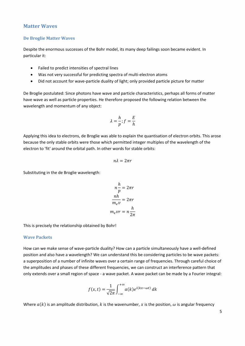
De Broglie postulated: Since photons have wave and particle characteristics, perhaps all forms of matter

have wave as well as particle properties. He therefore proposed the following relation between the

wavelength and momentum of any object:

Applying this idea to electrons, de Broglie was able to explain the quantisation of electron orbits. This arose

because the only stable orbits were those which permitted integer multiples of the wavelength of the

electron to 'fit' around the orbital path. In other words for stable orbits:

Substituting in the de Broglie wavelength:

This is precisely the relationship obtained by Bohr!

Wave Packets

How can we make sense of wave-particle duality? How can a particle simultaneously have a well-defined

position and also have a wavelength? We can understand this be considering particles to be wave packets:

a superposition of a number of infinite waves over a certain range of frequencies. Through careful choice of

the amplitudes and phases of these different frequencies, we can construct an interference pattern that

only extends over a small region of space - a wave packet. A wave packet can be made by a Fourier integral:

Where is an amplitude distribution, is the wavenumber, is the position, is angular frequency

6

Group Velocity and Phase Velocity

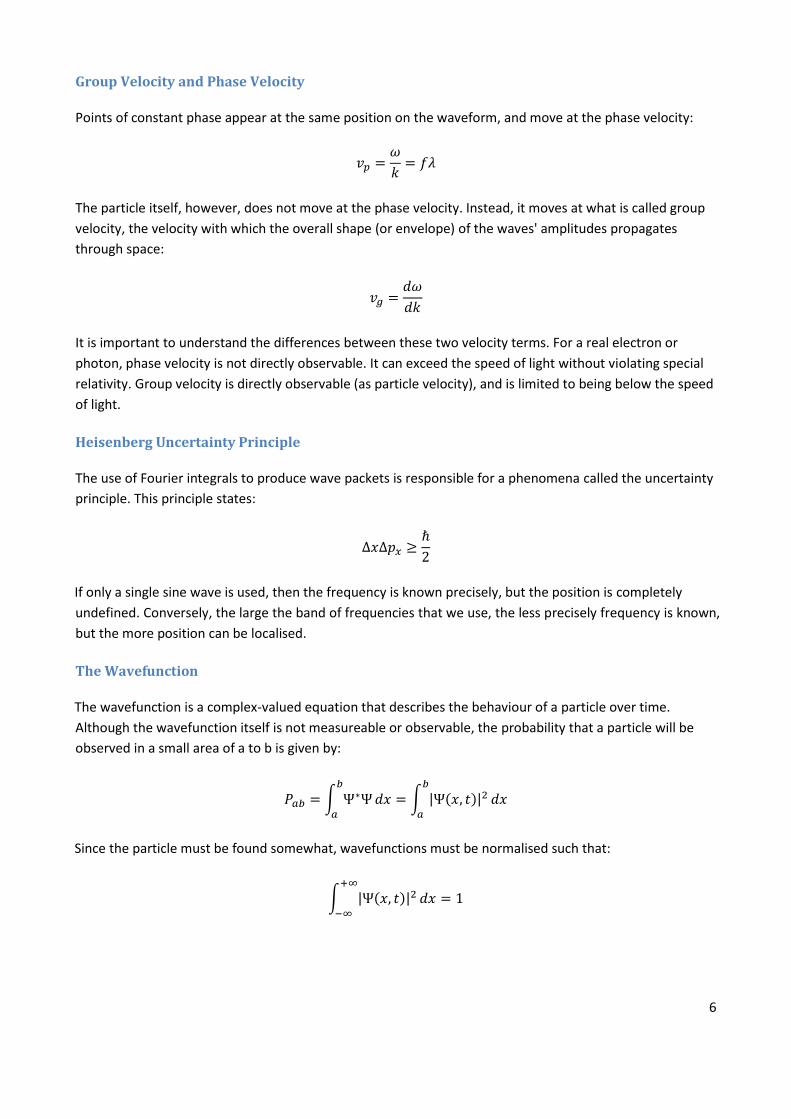
Points of constant phase appear at the same position on the waveform, and move at the phase velocity:

The particle itself, however, does not move at the phase velocity. Instead, it moves at what is called group

velocity, the velocity with which the overall shape (or envelope) of the waves' amplitudes propagates

through space:

It is important to understand the differences between these two velocity terms. For a real electron or

photon, phase velocity is not directly observable. It can exceed the speed of light without violating special

relativity. Group velocity is directly observable (as particle velocity), and is limited to being below the speed

of light.

Heisenberg Uncertainty Principle

The use of Fourier integrals to produce wave packets is responsible for a phenomena called the uncertainty

principle. This principle states:

If only a single sine wave is used, then the frequency is known precisely, but the position is completely

undefined. Conversely, the large the band of frequencies that we use, the less precisely frequency is known,

but the more position can be localised.

The Wavefunction

The wavefunction is a complex-valued equation that describes the behaviour of a particle over time.

Although the wavefunction itself is not measureable or observable, the probability that a particle will be

observed in a small area of a to b is given by:

Since the particle must be found somewhat, wavefunctions must be normalised such that:

7

Quantum Mechanics in One Dimension

The Schrodinger Equation

The Schrödinger equation is a partial differential equation that describes how the quantum state of some

physical system changes with time. The wave function is the most complete description that can be given

to a physical system. It is analogous to Newton's laws of motion in classical mechanics.

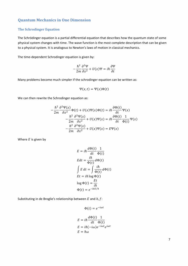
The time-dependent Schrodinger equation is given by:

Many problems become much simpler if the schrodinger equation can be written as:

We can then rewrite the Schrodinger equation as:

Where is given by

Substituting in de Broglie's relationship between and :

8

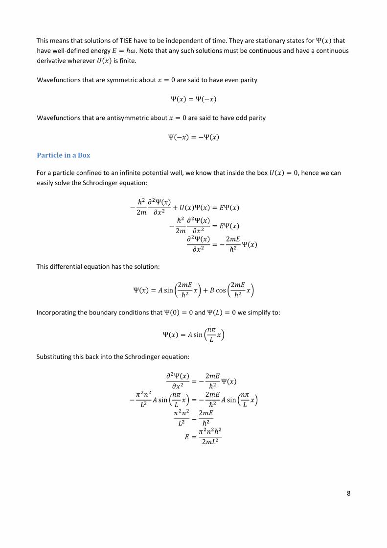
This means that solutions of TISE have to be independent of time. They are stationary states for that

have well-defined energy . Note that any such solutions must be continuous and have a continuous

derivative wherever is finite.

Wavefunctions that are symmetric about are said to have even parity

Wavefunctions that are antisymmetric about are said to have odd parity

Particle in a Box

For a particle confined to an infinite potential well, we know that inside the box , hence we can

easily solve the Schrodinger equation:

This differential equation has the solution:

Incorporating the boundary conditions that and we simplify to:

Substituting this back into the Schrodinger equation:

9

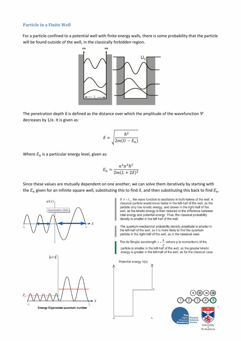
Particle in a Finite Well

For a particle confined to a potential well with finite energy walls, there is some probability that the particle

will be found outside of the well, in the classically forbidden region.

The penetration depth δ is defined as the distance over which the amplitude of the wavefunction

decreases by 1/e. It is given as:

Where is a particular energy level, given as:

Since these values are mutually dependent on one another, we can solve them iteratively by starting with

the given for an infinite square well, substituting this to find , and then substituting this back to find .

10

Wavefunction Summary

For the common cases of an infinite potential well, finite potential well, and finite square barrier,

Schrodinger's equation simplifies to:

If the sign is positive, the solutions will be of the form:

If the sign is negative, the solutions will instead be of the form:

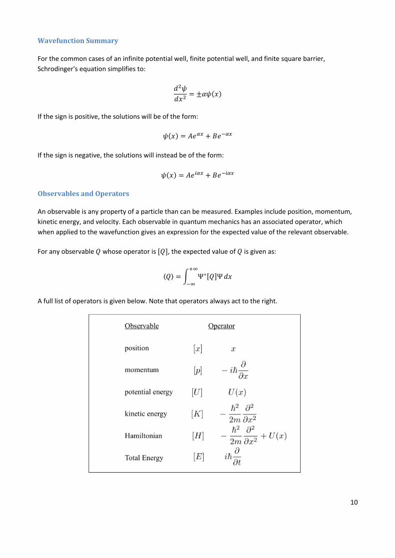
Observables and Operators

An observable is any property of a particle than can be measured. Examples include position, momentum,

kinetic energy, and velocity. Each observable in quantum mechanics has an associated operator, which

when applied to the wavefunction gives an expression for the expected value of the relevant observable.

For any observable whose operator is , the expected value of is given as:

A full list of operators is given below. Note that operators always act to the right.

11

Eigenvalues and Eigenfunctions

The quantum uncertainty for any observable is defined as:

If , we say that is a sharp observable, and all measurements of for a given system obtain the

same value. Otherwise, measurement will yield a distribution of values.

It turns out that for to be sharp, the wavefunction must be an eigenfunction of the operator . The

eigenvalue will then be the sharp value of . The wavefunction is an eigenfunction of if:

Also note that in general, the order in which operators act matters. If the order does not matter, then the

operators are said to commuate. This will be the case when:

If two operators do not commuate, the difference between them is called a commutator:

A further interesting result is that if two operators do not commute then the associated observables

cannot be simultaneously measured precisely and the commutator is related to the product of the

uncertainties.

Tunneling Phenomena

Classically, if the particle energy is less than the energy of a potential barrier , then we expect the

particle to be reflected off the barrier. In quantum mechanics, however, no region is inaccessible to a

particle regardless of its energy. Instead, the probability of a particle being found in a region of high

simply declines to very low levels.

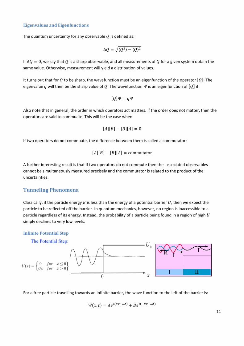
Infinite Potential Step

For a free particle travelling towards an infinite barrier, the wave function to the left of the barrier is:

12

The wave function to the right of the barrier consists of only a single term, since it travels only away from

the barrier:

Where

The boundary conditions for continuous wavefunctions require that , while continuous

derivatives require that . Hence we have:

The reflection coefficient is defined as:

Therefore, if , then all particles are totally reflected for an infinite potential step. Classically the

probability of reflection is zero if , and one if .

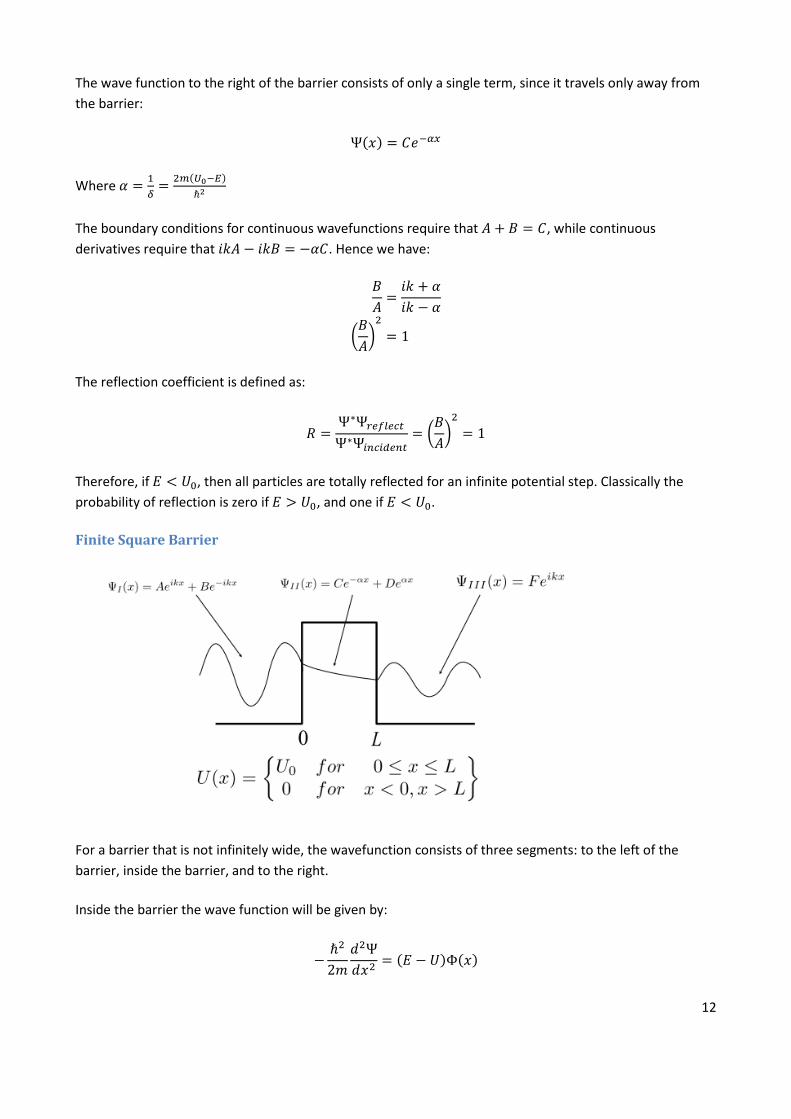
Finite Square Barrier

For a barrier that is not infinitely wide, the wavefunction consists of three segments: to the left of the

barrier, inside the barrier, and to the right.

Inside the barrier the wave function will be given by:

13

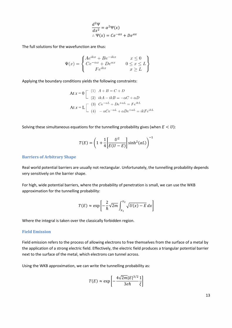
The full solutions for the wavefunction are thus:

Applying the boundary conditions yields the following constraints:

Solving these simultaneous equations for the tunnelling probability gives (when ):

Barriers of Arbitrary Shape

Real world potential barriers are usually not rectangular. Unfortunately, the tunnelling probability depends

very sensitively on the barrier shape.

For high, wide potential barriers, where the probability of penetration is small, we can use the WKB

approximation for the tunnelling probability:

Where the integral is taken over the classically forbidden region.

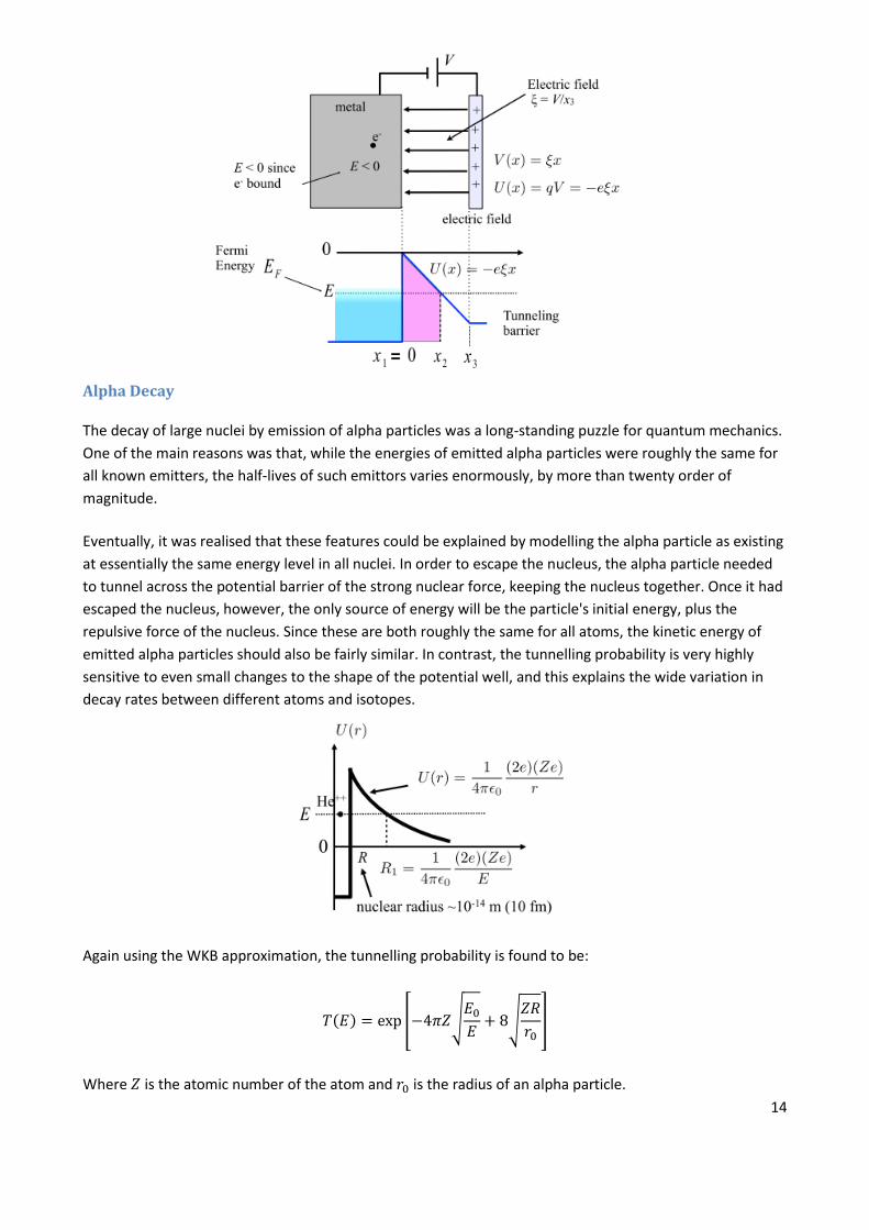
Field Emission

Field emission refers to the process of allowing electrons to free themselves from the surface of a metal by

the application of a strong electric field. Effectively, the electric field produces a triangular potential barrier

next to the surface of the metal, which electrons can tunnel across.

Using the WKB approximation, we can write the tunnelling probability as:

14

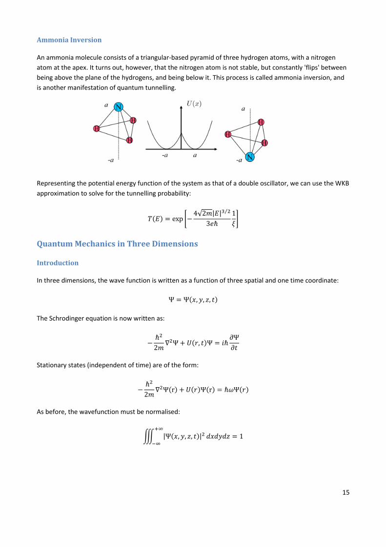
Alpha Decay

The decay of large nuclei by emission of alpha particles was a long-standing puzzle for quantum mechanics.

One of the main reasons was that, while the energies of emitted alpha particles were roughly the same for

all known emitters, the half-lives of such emittors varies enormously, by more than twenty order of

magnitude.

Eventually, it was realised that these features could be explained by modelling the alpha particle as existing

at essentially the same energy level in all nuclei. In order to escape the nucleus, the alpha particle needed

to tunnel across the potential barrier of the strong nuclear force, keeping the nucleus together. Once it had

escaped the nucleus, however, the only source of energy will be the particle's initial energy, plus the

repulsive force of the nucleus. Since these are both roughly the same for all atoms, the kinetic energy of

emitted alpha particles should also be fairly similar. In contrast, the tunnelling probability is very highly

sensitive to even small changes to the shape of the potential well, and this explains the wide variation in

decay rates between different atoms and isotopes.

Again using the WKB approximation, the tunnelling probability is found to be:

Where is the atomic number of the atom and is the radius of an alpha particle.

15

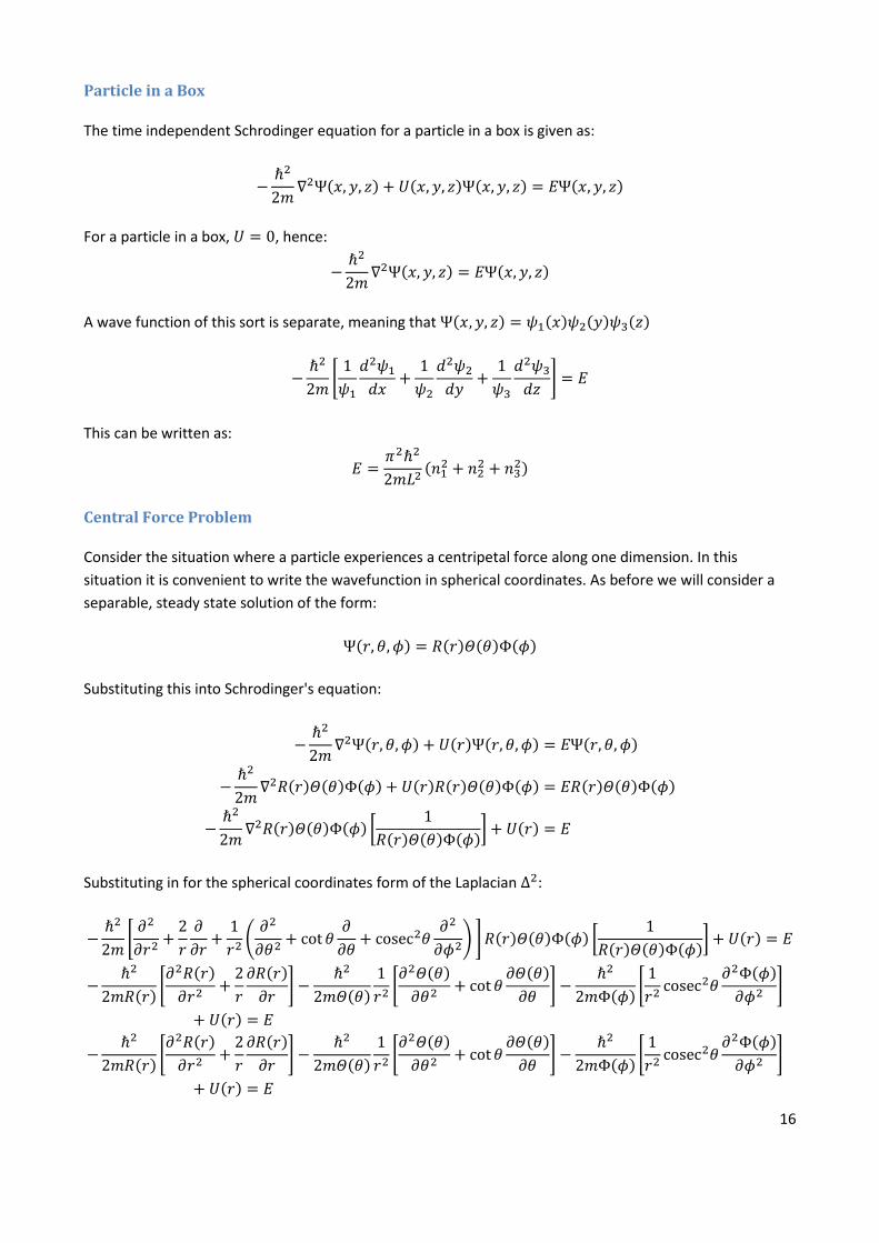
Ammonia Inversion

An ammonia molecule consists of a triangular-based pyramid of three hydrogen atoms, with a nitrogen

atom at the apex. It turns out, however, that the nitrogen atom is not stable, but constantly 'flips' between

being above the plane of the hydrogens, and being below it. This process is called ammonia inversion, and

is another manifestation of quantum tunnelling.

Representing the potential energy function of the system as that of a double oscillator, we can use the WKB

approximation to solve for the tunnelling probability:

Quantum Mechanics in Three Dimensions

Introduction

In three dimensions, the wave function is written as a function of three spatial and one time coordinate:

The Schrodinger equation is now written as:

Stationary states (independent of time) are of the form:

As before, the wavefunction must be normalised:

16

Particle in a Box

The time independent Schrodinger equation for a particle in a box is given as:

For a particle in a box, , hence:

A wave function of this sort is separate, meaning that

This can be written as:

Central Force Problem

Consider the situation where a particle experiences a centripetal force along one dimension. In this

situation it is convenient to write the wavefunction in spherical coordinates. As before we will consider a

separable, steady state solution of the form:

Substituting this into Schrodinger's equation:

Substituting in for the spherical coordinates form of the Laplacian :

17

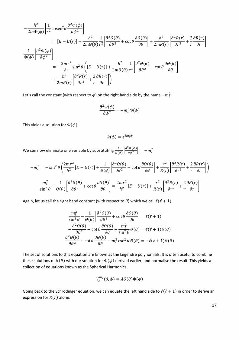
Let's call the constant (with respect to ) on the right hand side by the name

This yields a solution for :

We can now eliminate one variable by substituting

Again, let us call the right hand constant (with respect to ) which we call

The set of solutions to this equation are known as the Legendre polynomials. It is often useful to combine

these solutions of with our solution for derived earlier, and normalise the result. This yields a

collection of equations known as the Spherical Harmonics.

Going back to the Schrodinger equation, we can equate the left hand side to in order to derive an

expression for alone:

18

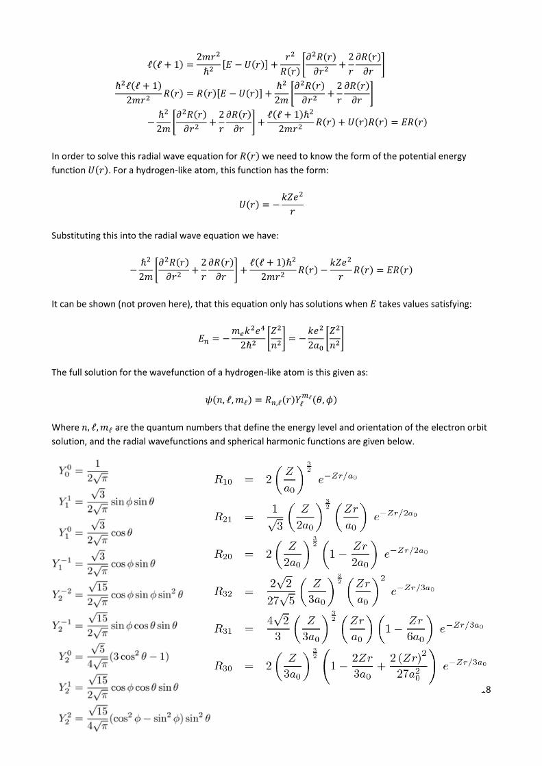
In order to solve this radial wave equation for we need to know the form of the potential energy

function . For a hydrogen-like atom, this function has the form:

Substituting this into the radial wave equation we have:

It can be shown (not proven here), that this equation only has solutions when takes values satisfying:

The full solution for the wavefunction of a hydrogen-like atom is this given as:

Where are the quantum numbers that define the energy level and orientation of the electron orbit

solution, and the radial wavefunctions and spherical harmonic functions are given below.

19

As an example, the ground state for a hydrogen-like atom is given by:

Special Relativity

Inertial Reference Frames

All inertial frames are in a state of constant, linear motion with respect to one another; an

accelerometer moving with any of them would detect zero acceleration

Fictitious forces arise from non-uniform relative motion between the two frames of reference

An inertial frame of reference is one in which fictitious forces are absent

The laws of physics are the same in all inertial frames

Lorentz Transformations

Lorentz transformations are a set of coordinate transformation equations which describe how

measurements of space and time vary from one reference frame to another. Maxwell's equations of

electromagnetism are invariant under the Lorentz transformations, which means that all observers will

agree on these laws of physics. Distance and time intervals are not invariant under lorentz transformations,

hence the term 'relativity'.

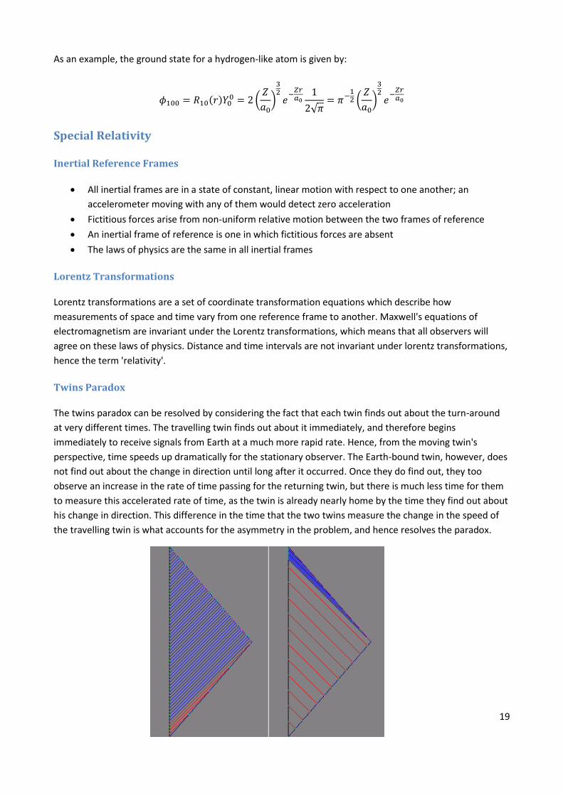
Twins Paradox

The twins paradox can be resolved by considering the fact that each twin finds out about the turn-around

at very different times. The travelling twin finds out about it immediately, and therefore begins

immediately to receive signals from Earth at a much more rapid rate. Hence, from the moving twin's

perspective, time speeds up dramatically for the stationary observer. The Earth-bound twin, however, does

not find out about the change in direction until long after it occurred. Once they do find out, they too

observe an increase in the rate of time passing for the returning twin, but there is much less time for them

to measure this accelerated rate of time, as the twin is already nearly home by the time they find out about

his change in direction. This difference in the time that the two twins measure the change in the speed of

the travelling twin is what accounts for the asymmetry in the problem, and hence resolves the paradox.

20

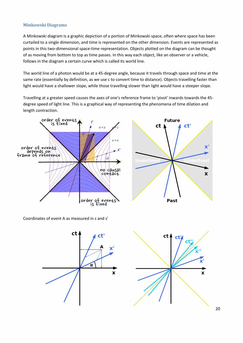
Minkowski Diagrams

A Minkowski diagram is a graphic depiction of a portion of Minkowski space, often where space has been

curtailed to a single dimension, and time is represented on the other dimension. Events are represented as

points in this two-dimensional space-time representation. Objects plotted on the diagram can be thought

of as moving from bottom to top as time passes. In this way each object, like an observer or a vehicle,

follows in the diagram a certain curve which is called its world line.

The world line of a photon would be at a 45-degree angle, because it travels through space and time at the

same rate (essentially by definition, as we use c to convert time to distance). Objects travelling faster than

light would have a shallower slope, while those travelling slower than light would have a steeper slope.

Travelling at a greater speed causes the axes of one's reference frame to 'pivot' inwards towards the 45-

degree speed of light line. This is a graphical way of representing the phenomena of time dilation and

length contraction.

Coordinates of event A as measured in s and s'

21

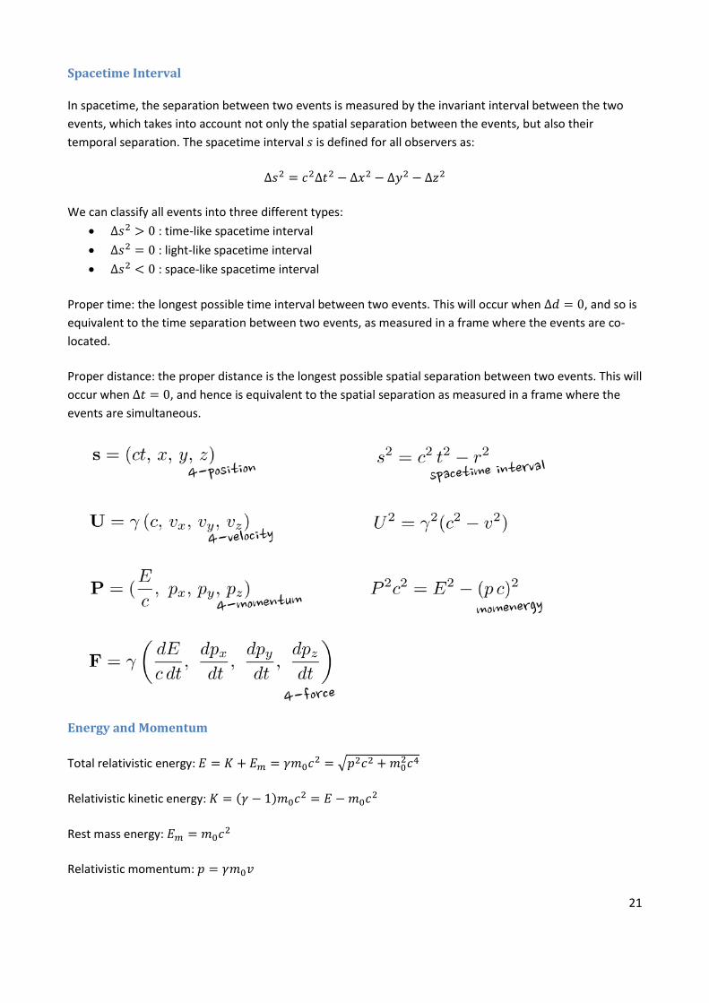
Spacetime Interval

In spacetime, the separation between two events is measured by the invariant interval between the two

events, which takes into account not only the spatial separation between the events, but also their

temporal separation. The spacetime interval is defined for all observers as:

We can classify all events into three different types:

: time-like spacetime interval

: light-like spacetime interval

: space-like spacetime interval

Proper time: the longest possible time interval between two events. This will occur when , and so is

equivalent to the time separation between two events, as measured in a frame where the events are co-

located.

Proper distance: the proper distance is the longest possible spatial separation between two events. This will

occur when , and hence is equivalent to the spatial separation as measured in a frame where the

events are simultaneous.

Energy and Momentum

Total relativistic energy:

Relativistic kinetic energy:

Rest mass energy:

Relativistic momentum: