Quantum theory of a bandpass Purcell filter for qubit readout
Eyob A. Sete,1,* John M. Martinis,2,3 and Alexander N. Korotkov1
1Department of Electrical and Computer Engineering, University of California, Riverside, California 92521, USA2Department of Physics, University of California, Santa Barbara, California 93106, USA
3Google Inc., Santa Barbara, California, USA(Received 22 April 2015; published 21 July 2015)
The measurement fidelity of superconducting transmon and Xmon qubits is partially limited by the qubitenergy relaxation through the resonator into the transmission line, which is also known as the Purcell effect. Oneway to suppress this energy relaxation is to employ a filter which impedes microwave propagation at the qubitfrequency. We present semiclassical and quantum analyses for the bandpass Purcell filter realized by E. Jeffreyet al. [Phys. Rev. Lett. 112, 190504 (2014)]. For typical experimental parameters, the bandpass filter suppressesthe qubit relaxation rate by up to two orders of magnitude while maintaining the same measurement rate. Wealso show that in the presence of a microwave drive the qubit relaxation rate further decreases with increasingdrive strength.
The implementation of fault-tolerant quantum informationprocessing [1] requires high-fidelity quantum gates and alsoneeds sufficiently fast and accurate qubit measurement. Super-conducting quantum computing technology [2–10] is currentlyapproaching the threshold for quantum error correction.Compared with the recent rapid progress in the increase ofsingle-qubit and two-qubit gate fidelities, qubit measurementshows somewhat slower progress. The development of fasterand higher-fidelity qubit readout remains an important task.
In circuit QED (cQED) [11,12] the qubit state is inferredby measuring the state-dependent frequency shift of theresonator via homodyne detection. This method introducesan unwanted decay channel [13] for the qubit due to theenergy leakage through the resonator into the transmission line,the process known as the Purcell effect [14,15]. The Purcelleffect is one of the limiting factors for high fidelity qubitreadout.
In principle, the Purcell rate can be suppressed by increasingthe qubit-resonator detuning, decreasing the qubit-resonatorcoupling, or decreasing the resonator bandwidth due todamping. However, these simple methods increase the timeneeded to measure the qubit. This leads to a trade-off betweenthe qubit relaxation and measurement time, whereas it isdesirable to suppress the Purcell rate without compromisingqubit measurement. Several proposals have been put forwardfor this purpose, which include employing a Purcell filter[16–19], engineering a Purcell-protected qubit [20,21], orusing a tunable coupler that decouples the transmission linefrom the resonator during the qubit-resonator interaction,thereby avoiding the Purcell effect altogether [22].
The general idea of the Purcell filter is to impede thepropagation of the photon emitted at the qubit frequency,compared with propagation of the microwave field at theresonator frequency, used for the qubit measurement. A notch
*Present address: Rigetti Quantum Computing, 2855 Telegraph Ave,Berkeley, CA 94705, USA.
(band-rejection) filter detuned by 1.7 GHz from the resonatorfrequency was realized in Ref. [16]. A factor of 50 reductionin the Purcell rate was demonstrated when the qubit frequencywas placed in the rejection band of the filter. A bandpassfilter with the quality factor Qf � 30 (and correspondingbandwidth of 0.22 GHz) centered near the resonator frequencywas used in Ref. [17]. This allowed the qubit measurementwithin 140 ns with fidelities F|1〉 = 98.7 and F|0〉 = 99.3 forthe two qubit states. (The bandpass Purcell filter was alsoused in Ref. [10]; it had a similar design with a few minorchanges.) A major advantage of the bandpass Purcell filterin comparison with the notch filter is the possibility to keepstrongly reduced Purcell rate for qubits with practically anyfrequency (except near the filter frequency), thus allowingquantum gates based on tuning the qubit frequency, and alsoallowing multiplexed readout of several qubits by placingreadout resonators with different frequencies within the filterbandwidth.
In this work we analyze the Purcell filter of Ref. [17] usingboth semiclassical and quantum approaches and consideringboth the weak and the strong drive regimes. Our semiclassicalanalysis uses somewhat different language compared to theanalysis in Ref. [17]; however, the results are very similar (theyshow that with the filter the Purcell rate can be suppressedby two orders of magnitude, while maintaining the samemeasurement time). The results of the quantum analysis in theregime of a weak measurement drive or no drive (consideringthe single-photon subspace) practically coincide with thesemiclassical results. In the presence of strong microwavedrive, the Purcell rate is further suppressed with increasingdrive strength. We have found that this suppression is strongerthan that obtained without a filter [23].
In Sec. II we discuss the general idea of the bandpass Purcellfilter and analyze its operation semiclassically. Section IIIis devoted to the quantum calculation of the Purcell ratein the presence of the bandpass Purcell filter. In Sec. IVwe discuss further suppression of the Purcell rate due to anapplied microwave drive. Section V is the conclusion. In theAppendix we review the basic theory of a transmon/Xmonqubit measurement, the Purcell decay, and the correspondingmeasurement error without the Purcell filter.
SETE, MARTINIS, AND KOROTKOV PHYSICAL REVIEW A 92, 012325 (2015)
FIG. 1. (Color online) Schematic of a standard circuit QED qubitreadout setup. The qubit state slightly changes the resonator frequencyωr (due to qubit-resonator interaction with strength g), and this issensed by passing the microwave through (or reflecting from) theresonator. The amplified outgoing microwave is combined with thelocal oscillator at the mixer, whose output is measured to discriminatethe qubit states. The energy decay κ of the resonator is mainly due toits coupling with the transmission line.
II. IDEA OF A BANDPASS PURCELL FILTERAND SEMICLASSICAL ANALYSIS
In the standard cQED setup of dispersive measurement(Fig. 1) the qubit interaction with the resonator slightly changesthe effective resonator frequency depending on the qubit state,so that it is ω
|e〉r when the qubit is in the excited state and ω
|g〉r
when the qubit is in the ground state. The dispersive couplingχ is defined as
χ ≡ (ω|e〉
r − ω|g〉r
)/2. (1)
In the two-level approximation for the qubit, χ=g2/(ωbq − ωb
r ),where g is the qubit-resonator coupling and ωb
q and ωbr
are the bare frequencies of the qubit and the resonator,respectively [11]. For a transmon or an Xmon qubit, χ
is usually significantly smaller, χ ≈ −g2δq/[(ωbq − ωb
r )(ωbq −
δq − ωbr )], where δq is the qubit anharmonicity (δq > 0);
moreover, χ as well as the central frequency (ω|e〉r + ω
|g〉r )/2
depend on the number of photons n in the resonator (see[24,25] and the Appendix for a more detailed discussion).The resonator frequency change (and thus the qubit state) issensed by applying the microwave field with amplitude ε, thenamplifying the transmitted or reflected signal, and then mixingit with the applied microwave field to measure its phase andamplitude (Fig. 1).
In the process of measurement, the qubit decays with thePurcell rate [11]
� ≈ κg2
(ωq − ωr)2, (2)
where κ is the resonator energy damping rate (mostly dueto leakage into the transmission line, see Fig. 1). Note thatin this formula we do not distinguish the bare and effectivefrequencies. In the quantum language this can be interpretedas the leakage with the rate κ of the qubit “tail” g2/(ωq − ωr)2,existing in the form of the resonator photon. However, thePurcell decay also has a simple classical interpretation viathe resistive damping [13], essentially being a linear effect,in contrast to the dispersion (1)—see the Appendix for moredetails, including dependence of � on n [23].
FIG. 2. (Color online) Qubit measurement schematic with thebandpass Purcell filter of Ref. [17]. The readout resonator withfrequency ωr (which depends on the qubit state) is coupled (couplingG) with a filter resonator of frequency ωf , which decays intothe transmission line with the rate κf . The further processingof the outgoing microwave (not shown) is the same as in Fig. 1. Themicrowave drive can be applied either to the readout (εr) or to the filter(εf ) resonators. Coupling with the decaying filter resonator producesan effective decay rate κeff of the readout resonator, which dependson the drive frequency. As a result, for the measurement microwaveκeff = κr, while the qubit sees a much smaller value κeff = κq, thusleading to a suppression of the qubit Purcell decay by a factor κq/κr.
The Purcell decay leads to measurement error; therefore,it is important to reduce the rate �. This can be done bydecreasing the ratio g/|ωq − ωr|; however, this decreases χ
and thus increases the necessary measurement time tm (seeAppendix for more details). Another way to decrease � is touse a very small leakage rate κ; however, this also increasesthe measurement time tm because the ring-up and ring-downprocesses give a natural limitation tm � 4 κ−1, and in manypractical cases it is even tm � 10 κ−1.
It would be good if the rate κ which governs the mea-surement time were different from κ in Eq. (2): specificallyif κ for the Purcell decay were much smaller than κ for themeasurement. This is exactly what is achieved by using thebandpass filter of Ref. [17]. There are other ways to explainhow this Purcell filter works [17], but here we interpret themain idea of the bandpass Purcell filter as producing differenteffective rates κeff for the measurement and for the Purcelldecay (so that the measurement microwave easily passesthrough the filter, while the propagation of the photon emittedby the qubit is strongly impeded by the filter).
The schematic of the qubit measurement with the bandpassPurcell filter of Ref. [17] is shown in Fig. 2. Besides the readoutresonator with qubit-state-dependent frequency ωr = ω
|e〉r or
ωr = ω|g〉r , there is a second (filter) resonator with frequency ωf ,
coupled with the readout resonator with the coupling G. (Thecoupling G is inductive, but we draw it as capacitive to keep thefigure simple.) The filter resonator leaks the microwave intothe transmission line with a relatively large damping rate κf ,so that its Q factor is Qf = ωf/κf � 30, while |G| � κf . Theleaked field is then amplified and sent to the mixer (not shown)in the same way as in the standard cQED setup. The readout andfilter resonators are in general detuned from each other, but notmuch, |ωr − ωf| � κf (detuning is needed to multiplex readoutof several qubits using the same filter resonator [10,17]; forsimplicity we consider the measurement of only one qubit).The filter resonator is pumped with the drive frequency ωd
012325-2
QUANTUM THEORY OF A BANDPASS PURCELL FILTER . . . PHYSICAL REVIEW A 92, 012325 (2015)
(close to ωr) and amplitude εf . However, for us it will be easierto first assume instead that the readout resonator is pumpedwith amplitude εr (Fig. 2), and then show the correspondencebetween the drives εr and εf .
Let us use the rotating wave approximation [26,27] with therotating frame e−iωd t based on the drive frequency ωd. Thenthe evolution of the classical field amplitudes α(t) and β(t) inthe readout and filter resonators, respectively, is given by theequations
α = −irdα − iGβ − iεr, (3)
β = −ifdβ − iG∗α − κf
2β, (4)
where α and β are normalized so that |α|2 and |β|2 are theaverage number of photons in the resonators, εr is normalizedcorrespondingly, and
rd = ωr − ωd, fd = ωf − ωd (5)
(recall that ωr depends on the qubit state). If we are notinterested in the details of evolution on the fast time scaleκ−1
f , then we can use the quasisteady state for β [obtainedfrom Eq. (4) using β = 0],
β = −iG∗
κf/2 + ifdα, (6)
which can then be inserted into Eq. (3), giving
α = −i(rd + δωr) α − κeff
2α − iεr, (7)
κeff = 4|G|2κf
1
1 + (2fd/κf)2, (8)
δωr = − |G|2fd
(κf/2)2 + 2fd
= −fd
κfκeff . (9)
Thus we see that the field α evolves in practically the sameway as in the standard setup of Fig. 1; however, interactionwith the filter resonator shifts the readout resonator frequencyby δωr and introduces the effective leakage rate κeff of thereadout resonator.
Most importantly, κeff depends on the drive frequency. Formeasurement we use ωd ≈ ωr, so κeff is approximately
κr ≡ 4|G|2κf
1
1 + [2(ωr − ωf)/κf]2. (10)
However, when the qubit tries to leak its excitation throughthe readout resonator, this can be considered as a drive at thequbit frequency, ωd = ωq, and the corresponding κeff is then
κq ≡ 4|G|2κf
1
1 + [2(ωq − ωf)/κf]2, (11)
which is much smaller than κr if the qubit is detuned awayfrom the filter linewidth, |ωq − ωf| � κf . This difference isexactly what we wished for suppressing the Purcell rate �:the measurement is governed by κr, while the qubit sees amuch smaller value κq. Therefore, we would expect that thePurcell rate is given by Eq. (2) with κ = κq [see Eq. (32)later], while the “separation” measurement error is given byEqs. (A36)–(A38) with κ = κr (see Appendix). As a result,
compared with the standard setup (Fig. 1) with the samephysical parameters for measurement, the Purcell rate issuppressed by the factor
F = κq
κr= 1 + [2(ωr − ωf)/κf]2
1 + [2(ωq − ωf )/κf]2� 1. (12)
This is essentially the main result of this paper, which willbe confirmed by the quantum analysis in the next section. (Toavoid a possible confusion, we note that κq is not the qubitdecay rate; it is the resonator decay, as seen by the qubit.)
Our result for the Purcell suppression factor was based onthe behavior of the field amplitude in the readout resonator.Let us also check that the field γtl propagating in the outgoingtransmission line behaves according to the effective modelas well. The outgoing field amplitude is γtl = √
κf β (inthe normalization for which |γtl|2 is the average number ofpropagating photons per second). Using Eq. (6) we find
γtl = −iG∗√κf
κf/2 + ifdα = eiϕ√
κeff α, (13)
so, as expected, the outgoing amplitude behaves as in thestandard setup of Fig. 1 with κ = κeff , up to an unimportantphase shift ϕ = arg[−iG∗/(κf/2 + ifd)]. Note that to showthe equivalence between the dynamics (including transients)of the systems in Figs. 1 and 2 we needed the assumption ofa sufficiently large κf in order to use the quasisteady state (6).However, this assumption is not needed if we consider onlythe steady state (without transients).
So far we assumed that the measurement is performed bydriving the readout resonator with the amplitude εr. Now let usconsider the realistic case [10,17] when the drive εf is appliedto the filter resonator. The evolution equations (3) and (4) forthe classical field amplitudes are then replaced by
α = −irdα − iGβ, (14)
β = −ifdβ − iG∗α − κf
2β − iεf, (15)
so that the quasisteady state for the filter resonator is
β = −iG∗
κf/2 + ifdα + −iεf
κf/2 + ifd, (16)
and the field evolution in the readout resonator is
α = −i(rd + δωr) α − κeff
2α − G
κf/2 + ifdεf, (17)
with the same κeff and δωr given by Eqs. (8) and (9). The onlydifference between the effective evolution equations (7) and(17) is a linear relation,
εr ↔ −iεfG/(κf/2 + ifd), (18)
between the drive amplitudes εr and εf producing the sameeffect. Therefore, our results obtained above remain unchangedfor driving the filter resonator, and the Purcell rate suppressionfactor is still given by Eq. (12).
Note that in the quasisteady state the separation between thefilter amplitudes β for the two qubit states does not depend onwhether the drive is applied to the filter or readout resonator,as long as we use the correspondence (18) between the driveamplitudes. The same is true for the separation betweenthe outgoing fields γtl. Similarly, the separation between the
012325-3
SETE, MARTINIS, AND KOROTKOV PHYSICAL REVIEW A 92, 012325 (2015)
outgoing fields for the two qubit states is the same (up tothe phase ϕ) as in the standard setup of Fig. 1 with ε = εr,κ = κr, and the resonator frequency adjusted by δωr givenby Eq. (9). Therefore, these configurations are equivalent toeach other from the point of view of quantum measurement,including interaction between the qubit and readout resonator,extraction of quantum information, back-action, etc.
Nevertheless, driving the filter resonator produces a dif-ferent outgoing field γtl = √
κf β, which now contains anadditional term −iεf
√κf/(κf/2 + ifd) in comparison with
Eq. (13), which comes from the second term in Eq. (16). Inparticular, instead of the Lorentzian line shape of the transferfunction when driving the readout resonator, the transferfunction for driving the filter is (in the steady state)
γ(f)tl
εf=
√κf
κf/2 + ifd
2rd/κeff
1 + 2i(rd + δωr)
κeff
, (19)
where κeff can be replaced with κr. (Note a nonstandardnormalization of the transfer function because of differentnormalizations of γ
(f)tl and εf .) This line shape for the amplitude
|γ (f)tl /εf| shows a dip near ωr (note that γ
(f)tl /εf = 0 at ωd = ωr)
and is significantly asymmetric when δωr is comparable to κr;this occurs when the detuning between the readout and filterresonators is comparable to κf—see Eq. (9). In terms of thefield α in the readout resonator, the outgoing field at steadystate is
γ(f)tl = −
√κf rd
G α (20)
instead of Eq. (13) for driving the readout resonator.The difference between the outgoing fields γ
(f)tl and γ
(r)tl
when driving the filter or readout resonator (for the sameα, i.e., the same measurement conditions) may be importantfor saturation of the microwave amplifier. The ratio of thecorresponding outgoing powers is∣∣γ (f)
tl
∣∣2∣∣γ (r)tl
∣∣2 =(
rd
κr
)2 4
1 + (2fd/κf)2, (21)
where we assumed |rd| � κf (so that κeff ≈ κr). For example,if the drive frequency is chosen as ωd = (ω|g〉
r + ω|e〉r )/2, then
rd = ±χ ; if in this case |χ | � κr, then driving the filterresonator is advantageous because it produces less power to beamplified, while driving the readout resonator is advantageousif |χ | � κr. However, when ωd �= (ω|g〉
r + ω|e〉r )/2, the situation
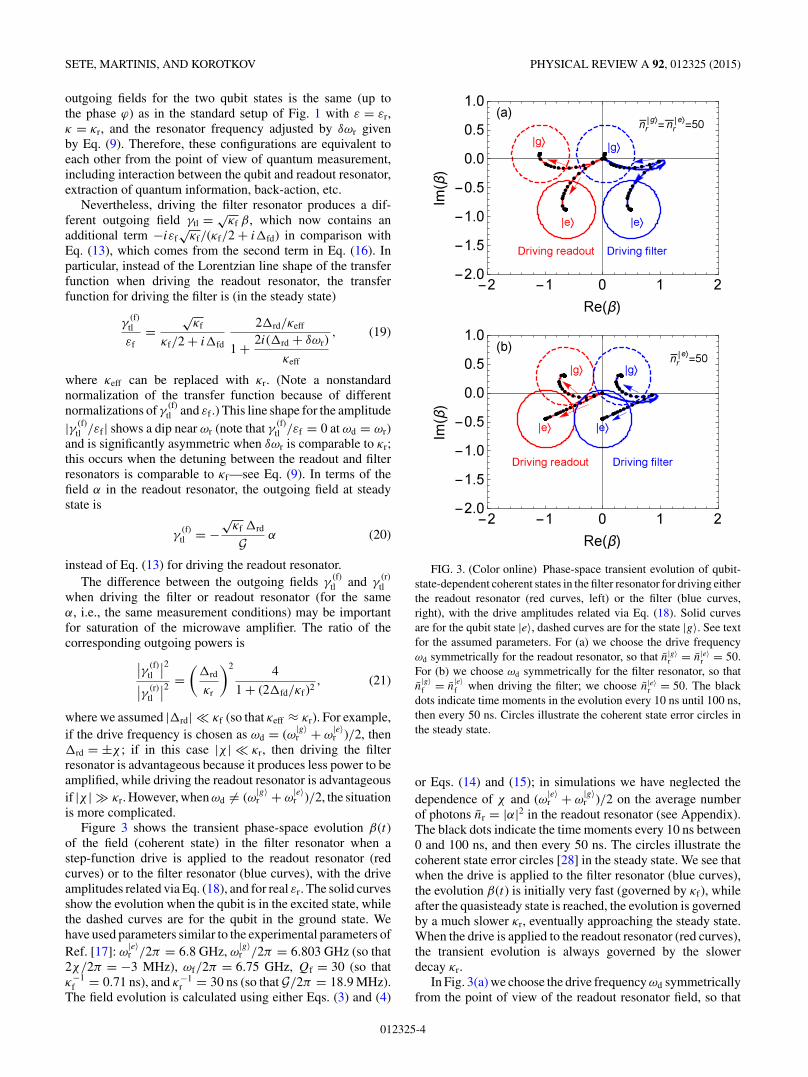
is more complicated.Figure 3 shows the transient phase-space evolution β(t)
of the field (coherent state) in the filter resonator when astep-function drive is applied to the readout resonator (redcurves) or to the filter resonator (blue curves), with the driveamplitudes related via Eq. (18), and for real εr. The solid curvesshow the evolution when the qubit is in the excited state, whilethe dashed curves are for the qubit in the ground state. Wehave used parameters similar to the experimental parameters ofRef. [17]: ω
f = 0.71 ns), and κ−1r = 30 ns (so that G/2π = 18.9 MHz).
The field evolution is calculated using either Eqs. (3) and (4)
FIG. 3. (Color online) Phase-space transient evolution of qubit-state-dependent coherent states in the filter resonator for driving eitherthe readout resonator (red curves, left) or the filter (blue curves,right), with the drive amplitudes related via Eq. (18). Solid curvesare for the qubit state |e〉, dashed curves are for the state |g〉. See textfor the assumed parameters. For (a) we choose the drive frequencyωd symmetrically for the readout resonator, so that n|g〉
r = n|e〉r = 50.
For (b) we choose ωd symmetrically for the filter resonator, so thatn
|g〉f = n
|e〉f when driving the filter; we choose n|e〉
r = 50. The blackdots indicate time moments in the evolution every 10 ns until 100 ns,then every 50 ns. Circles illustrate the coherent state error circles inthe steady state.
or Eqs. (14) and (15); in simulations we have neglected thedependence of χ and (ω|e〉
r + ω|g〉r )/2 on the average number
of photons nr = |α|2 in the readout resonator (see Appendix).The black dots indicate the time moments every 10 ns between0 and 100 ns, and then every 50 ns. The circles illustrate thecoherent state error circles [28] in the steady state. We see thatwhen the drive is applied to the filter resonator (blue curves),the evolution β(t) is initially very fast (governed by κf), whileafter the quasisteady state is reached, the evolution is governedby a much slower κr, eventually approaching the steady state.When the drive is applied to the readout resonator (red curves),the transient evolution is always governed by the slowerdecay κr.
In Fig. 3(a) we choose the drive frequency ωd symmetricallyfrom the point of view of the readout resonator field, so that
012325-4
QUANTUM THEORY OF A BANDPASS PURCELL FILTER . . . PHYSICAL REVIEW A 92, 012325 (2015)
in the steady state n|g〉r = n
|e〉r = 50, where n
|g〉r and n
|e〉r are
the average photon numbers for the two qubit states. For thatwe need ωd = (ω|g〉
r + ω|e〉r )/2 + δωr with δωr given by Eq. (9);
for our parameters δωr/2π = 1.23 MHz, so ωd/2π = 6.80273GHz. Such symmetric choice of the drive frequency providesthe largest separation between the two coherent states fora fixed drive amplitude if 2 |χ | < κr. While the field in thereadout resonator is always symmetric in this case, Fig. 3(a)shows that the field in the filter resonator is symmetric onlywhen driving the readout resonator (red curves, n
|g〉f = n
|e〉f =
1.2), while it is strongly asymmetric when the filter resonatoris driven (blue curves, n
|g〉f = 0.01, n
|e〉f = 1.0; n
|g〉f is very
small because for our parameters δωr ≈ |χ | and thereforeωd ≈ ω
|g〉r ). The number of photons in the filter is much less
than in the readout resonator because κf � κr.In Fig. 3(b) we choose ωd so that in the steady state
n|g〉f = n
|e〉f for driving the filter; this is the natural choice for
decreasing the microwave power to be amplified. This occursat ωd/2π = 6.80120, which is close to the expected value(ω|g〉
r + ω|e〉r )/2, but not equal because of the asymmetry of the
line shape (19). We choose the amplitudes to produce n|e〉r = 50
(then n|g〉r = 22). The difference between n
|e〉r and n
|g〉r leads to
different values n|e〉f = 1.2 and n
|g〉f = 0.5 when driving the
readout resonator, while for driving the filter the field in thefilter is symmetric, n
|e〉f = n
|g〉f = 0.2. Compared to the case of
Fig. 3(a), there is 5 times less power to be amplified for the |e〉state (when driving the filter); however, the state separation is1.3 times smaller (in amplitude) for the same n
|e〉r . Thus, there
is a trade-off between the state separation and amplified powerin choosing the drive frequency. Comparing the red and bluecurves in Fig. 3(b), we see that in the steady state n
|g〉f and
n|e〉f are smaller for driving the filter rather than the readout
resonator. This is beneficial because there is less power to beamplified; however, the ratio is not very big (as expected for amoderate value |χ |/κr = 0.28).
Note that our definition of κr in Eq. (10) is not strictly welldefined because the resonator frequency ωr depends on thequbit state, and the drive frequency can be in between ω
|e〉r and
ω|g〉r . However, this frequency difference is much smaller than
κf , and therefore not important for practical purposes in thedefinition of κr. In an experiment κr can be measured eithervia the field decay [17] or via the linewidth of the steady-statetransfer function showing the dip of |γ (f)
tl /εf| near the resonanceωd = ωr [Eq. (19)], since near the dip κeff ≈ κr.
Thus far we assumed that all decay κf in the filter resonatoris due to the leakage κout
f into the outgoing transmission line.If κout
f < κf and the decay κf − κoutf is due to leakage into
the line delivering the drive εf or due to another dissipationchannel, then the only difference compared to the previousdiscussion is the extra factor
√κout
f /κf for the outgoing fieldγtl. This will lead to multiplication of the overall quantumefficiency of the measurement by κout
f /κf and will onlyslightly affect the measurement fidelity. Adding dissipationin the readout resonator with rate κr,d increases the effectivelinewidth to κeff + κr,d and multiplies the quantum efficiencyby κr/(κr + κr,d). Most importantly, since κr,d does not changewith frequency, the Purcell suppression factor (12) becomes
(κq + κr,d)/(κr + κr,d), so that the Purcell filter performancedeteriorates; we will discuss this in a little more detailin Sec. III C.
Note that our main result (12) for the Purcell suppressionfactor is slightly different from the result F = [κf/2(ωq −ωr)]2(ωq/ωr)2, which was derived in Ref. [17] using thecircuit theory. The reasons are the following. First, in thederivation of [17] it was assumed that the two resonatorshave the same frequency, which makes the numerator inEq. (12) equal to 1. Second, the term 1 in the denominatorin Eq. (12) was essentially neglected in comparison with thelarger second term. Finally, the role of the factor (ωq/ωr)2 is notquite clear. In the derivation of Ref. [17] keeping this factorwas exceeding the accuracy of the derivation, while in ourderivation we essentially use the rotating wave approximation,which assumes ωq/ωr ≈ 1. Aside from these small differences,our result coincides with the result of Ref. [17].
III. QUANTUM ANALYSIS INSINGLE-EXCITATION SUBSPACE
In this section we discuss the quantum derivation of thePurcell rate in the presence of the bandpass filter in theregime when the resonators are not driven or driven sufficientlyweakly to neglect dependence of the Purcell rate on thenumber of photons in the resonator [23]. More precisely,we consider the quantum evolution in the single-excitation(and zero-excitation) subspace. We apply two methods: thewave function approach, in which we use a non-HermitianHamiltonian with a decaying wave function, and the moretraditional density matrix analysis.
In the absence of the drive and in the rotating waveapproximation, the relevant Hamiltonian of the system shownin Fig. 2 (without considering decay κf) is (� = 1)
H = ωbqσ+σ− + ωb
r a†a + ωfb
†b + g(a†σ− + aσ+)
+Ga†b + G∗ab†, (22)
where ωbq is the bare qubit frequency, ωb
r is the bare frequencyof the readout resonator, ωf is the filter resonator frequency,raising/lowering operators σ+ and σ− act on the qubit state,a† and a are the creation and annihilation operators for thereadout resonator, b† and b are for the filter resonator, g isthe qubit-readout resonator coupling, and G is the resonator-resonator coupling. For simplicity we assume a real positiveg, but G can be complex for generality (for the capacitive orinductive coupling between the resonators, G is real if the samegeneralized coordinates are used for both resonators).
Note that in the case without drive it is sufficient to consideronly two levels for the qubit because only the single-excitation(and zero-excitation) subspace is involved in the evolution,and therefore the amount of qubit nonlinearity due to theJosephson junction is irrelevant. However, in the presenceof a drive (considered in the next section) it is formallynecessary to take into account several levels in the qubit (asdone in the Appendix). Nevertheless, to leading order thePurcell rate is insensitive to this, because the Purcell decayis essentially a classical linear effect (see discussion in theAppendix). Also note that the laboratory-frame Hamiltonian
012325-5
SETE, MARTINIS, AND KOROTKOV PHYSICAL REVIEW A 92, 012325 (2015)
(22) assumes the rotating wave approximation (as in thestandard Jaynes-Cummings Hamiltonian), since it neglects the“counter-rotating” terms of the form a†σ+, aσ−, a†b†, and ab.This requires assumption that |ωb
q − ωbr |, |ωf − ωb
r |, g, and |G|are small compared to ωb
r .Let us choose the rotating frame with frequency ωb
q, i.e.,H0=ωb
q(σ+σ− + a†a + b†b); then the interaction HamiltonianV = H − H0 is
V = rqa†a + fqb
†b + g(a†σ− + aσ+) + Ga†b + G∗ab†,
(23)
where
rq = ωbr − ωb
q, fq = ωf − ωbq, (24)
and the interaction picture is equivalent to the Schrodingerpicture because exp(iH0t)V exp(−iH0t) = V , which is be-cause the starting Hamiltonian (22) already assumes therotating-wave approximation. The master equation for thedensity matrix ρ, which includes the damping κf of the filterresonator is
ρ = −i[V,ρ] + κf(bρb† − b†bρ/2 − ρb†b/2). (25)
In general, the bare basis is |jnm〉, where j represents thequbit states, while n and m represent the readout and filterresonator Fock states, respectively. However, in this sectionwe consider only the single-excitation (and zero-excitation)subspace, so only four bare states are relevant: |e〉 ≡ |e00〉,|r〉 = |g10〉, |f〉 = |g01〉, and |g〉 = |g00〉.
Note that the interaction hybridizes the bare states of thequbit and the resonators. (Hybridization of the readout res-onator mode is essentially what makes the qubit measurementpossible.) Therefore, when discussing the Purcell rate forthe qubit energy relaxation, we actually mean decay of theeigenstate, corresponding to the qubit excited state. This makesperfect sense experimentally, since manipulations of the qubitstate usually occur in the eigenbasis (adiabatically, comparedwith the qubit detuning from the resonator).
A. Method I: Decaying wave function
Instead of using the traditional density matrix language forthe description of the Purcell effect [15], it is easier to use thelanguage of wave functions, even in the presence of the decayκf [23]. Physically the wave functions can still be used becausein the single-excitation subspace unraveling of the Lindbladequation corresponds to only one “no relaxation” scenario(see, e.g., [29]), and therefore the wave function evolutionis nonstochastic. Another, more formal way to introduce thislanguage, is to rewrite the master equation (25) as [30,31]ρ = −i[Heff,ρ] + κfbρb†, where Heff = V − iκfb
†b/2 is aneffective non-Hermitian Hamiltonian. Next, the term κfbρb†
can be neglected because in the single-excitation subspaceit produces only an “incoming” contribution from higher-excitation subspaces, which are not populated. Therefore, inthe single-excitation subspace we can use ρ = −i[Heff,ρ].Equivalently, |ψ〉 = −iHeff|ψ〉, which describes the evolutionof the decaying wave function |ψ(t)〉 = ce(t)|e〉 + cr(t)|r〉 +cf(t)|f〉. Therefore, the probability amplitudes ce,r,f satisfy the
following equations:
ce = −igcr, (26)
cr = −irqcr − igce − iGcf, (27)
cf = −ifqcf − iG∗cr − (κf/2) cf, (28)
while the population ρgg of the zero-excitation state |g〉 evolvesas ρgg = κf|cff |2 or can be found as ρgg = 1 − |cee|2 − |crr|2 −|cff |2. Note that Eqs. (27) and (28) exactly correspond to theclassical equations (3) and (4) with rd replaced with rq, alsofd replaced with fq, and εr replaced with gce.
From the eigenvalues λe,r,f = −iωe,r,f − �e,r,f/2 of thematrix representing Eqs. (26)–(28), one can obtain the eigen-frequencies ωe,r,f and the corresponding decay rates �e,r,f .These eigenvalues can be found from the qubic equation
λ3 + λ2(irq + ifq + κf/2) + λ(−rqfq + |G|2 + g2
+ irqκf/2) + g2(ifq + κf/2) = 0. (29)
We are interested in the Purcell rate � = �e, which corre-sponds to the decay of the eigenstate close to |e〉. Since λe isclose to zero, in the first approximation we can neglect the termλ3 in Eq. (29), thus reducing it to the quadratic equation. Ifmore accuracy is needed, the equation can be solved iteratively,replacing λ3 with the value found in the previous iteration(the second iteration is usually sufficient).
Besides finding the Purcell rate � exactly or approximatelyfrom Eq. (29), we can find it approximately by using quasis-teady solutions of Eqs. (27) and (28), to a large extent followingthe classical derivation in the previous section. Assumingcf = 0 in Eq. (28), we find cf = −iG∗cr/(ifq + κf/2). Insert-ing this quasisteady value into Eq. (27) and assuming cr = 0,we find cr= − igce/[irq + |G|2/(ifq + κf/2)]. Substitutingthis quasisteady value into Eq. (26), we obtain
ce = − g2
irq + |G|2/(ifq + κf/2)ce = λece. (30)
Finally, we obtain the Purcell rate as � = −2Re(λe),
� = g2|G|2κf
2rq[(fq − |G|2/rq)2 + (κf/2)2]
(31)
≈ g2|G|2κf
2rq
[2
fq + (κf/2)2] = g2κq
2rq
, (32)
where κq is given by Eq. (11) and we assumed |G|2 � fqrq
to transform Eq. (31) into Eq. (32).The Purcell rate given by Eq. (32) is exactly what we
expected from the classical analysis in Sec. II: in the usualformula (2) we simply need to substitute κ with the readoutresonator decay rate κq seen by the qubit. Since the measure-ment is governed by a different decay rate κr, the effectivePurcell rate suppression factor is given by Eq. (12), as wasexpected. This confirms the results of the classical analysis inSec. II.
B. Method II: Density matrix analysis
We can also find the Purcell rate in a more traditionalway by writing the master equation (25) explicitly in the
012325-6
QUANTUM THEORY OF A BANDPASS PURCELL FILTER . . . PHYSICAL REVIEW A 92, 012325 (2015)
single-excitation subspace:
ρee = ig(ρer − ρre), (33)
ρer = −iqrρer − ig(ρrr − ρee) + iG∗ρef, (34)
ρef = −κf
2ρef − iqfρef + iGρer − igρrf, (35)
ρrr = −ig(ρer − ρre) − iGρfr + iG∗ρrf, (36)
ρrf = −κf
2ρrf + ifrρrf − iGρff + iG∗ρrr − igρef, (37)
ρff = −κfρff − iG∗ρrf + iGρfr. (38)
Note that ρgg = κfρff and ρee + ρrr + ρff + ρgg = 1 (however,we do not use these two equations for the derivation of thePurcell rate).
Using the quasisteady solutions of Eqs. (34)–(38), i.e.,assuming ρer = ρef = ρrr = ρrf = ρff = 0, we can obtain alengthy equation for ρer, which is proportional to ρee. If weuse the first-order expansion of this equation in the coupling g
and neglect g3 terms (there is no g2 contribution), then
ρer = ig
irq + |G|2/(ifq + κf/2)ρee, (39)
which has the form similar to Eq. (30). Substituting this ρer intoEq. (33), we obtain the evolution equation ρee = −�ρee with �
given exactly by Eq. (31). If we do not use the above-mentionedapproximation for the quasisteady ρer, then the result for thePurcell rate is slightly different and much lengthier,
� = g2|G|2κf[(rqfq − |G|2)2 + (
2rq + g2
)(κf/2)2
+ g2(2
fq + 2fqrq − |G|2) + g4]−1
. (40)
Thus the derivations based on the wave function and densitymatrix languages using the quasisteady-state approximationboth lead to practically the same result for the Purcell rate �.The most physically transparent result is given by Eq. (32),which corresponds to the semiclassical analysis in Sec. II andsimply replaces κ in Eq. (2) with κq seen by the qubit, incontrast to the measurement process, which is governed by κr.
As an example, let us use the parameters similar to thatin Ref. [17]: ωq/2π = 5.9 GHz, ωr/2π = 6.8 GHz, ωf/2π =6.75 GHz, Qf = 30 (so that κ−1
f = 0.71 ns), g/2π = 90 MHz,and κ−1
r = 30 ns (so that G/2π = 18.9 MHz). In this case theresonator decay [Eq. (11)] seen by the qubit is κ−1
q = 1.45 μs,the Purcell rate [Eq. (32)] is � = 1/(145 μs), and the Purcellrate suppression factor [Eq. (12)] is F = 30 ns/1.45 μs =(1 + 0.442)/(1 + 7.62) = 0.021.
Thus, for typical parameters the bandpass Purcell filtersuppresses the Purcell decay by a factor of ∼50. It is easy toincrease this factor to 100 by using ωq/2π = 5.5 GHz in theabove example; however, further decrease of the Purcell rate isnot needed for practical purposes, while increased resonator-qubit detuning decreases the dispersive shift 2χ (in the aboveexample 2χ/2π ≈ −3 MHz for the qubit anharmonicity of180 MHz, while for ωq/2π = 5.5 GHz the dispersive shiftbecomes twice less).
Note that for the parameters in the above example, Eq. (32)overestimates the exact solution for � via Eq. (29) by 5%,the same 5% for Eq. (31), and Eq. (40) overestimates thePurcell rate by 2%. The solution of Eq. (29) as a quadratic
equation neglecting λ3 gives �, which overestimates the exactsolution by 22%, while the second iteration is practically exact(−0.01%). The inaccuracies grow for smaller resonator-qubitdetuning (crudely as −2
rq ), but remain reasonably small in asufficiently wide range; for example, Eq. (32) overestimatesthe Purcell rate by 50% for ωq/2π = 6.5 GHz, i.e. detuningof 0.3 GHz.
C. Nonzero readout resonator damping
In the quantum evolution model (25) we have consideredonly the damping of the filter resonator with the rate κf . If thereis also an additional energy dissipation in the readout resonatorwith the rate κr,d (e.g., due to coupling with the transmissionline delivering the drive εr in Fig. 2), then the masterequation (25) should be replaced with
ρ = − i[V,ρ] + κf(bρb† − b†bρ/2 − ρb†b/2)
+ κr,d(aρa† − a†aρ/2 − ρa†a/2). (41)
In the wave-function-language derivation this leads to the extraterm −κr,dcr/2 in Eq. (27) for cr. This does not change thequasisteady value for cf but changes the quasisteady valuecr = −igce/[irq + |G|2/(ifq + κf/2) + κr,d/2], so that thePurcell rate is
� = 2 Re
[g2
irq + |G|2/(ifq + κf/2) + κr,d/2
](42)
≈ g2(κq + κr,d)
2rq
(43)
instead of Eq. (32). Practically the same result can be obtainedusing the derivation via the density matrix evolution (assumingκr,d � κf). As expected, the dissipation κr,d simply adds to therate κq seen by the qubit. Since κr,d is not affected by the filter, itadds in the same way to the bandwidth κr governing the qubitmeasurement process and thus deteriorates the Purcell ratesuppression (12), replacing it with F = (κq + κr,d)/(κr + κr,d).
IV. PURCELL RATE WITH MICROWAVE DRIVEAND BANDPASS FILTER
The Purcell rate may decrease when the measurementmicrowave drive is added [23]. A simple physical reason is theac Stark shift, which in the typical setup increases the absolutevalue of detuning between the qubit and readout resonator withincreasing number of photons in the resonator, thus reducingthe Purcell rate. However, this explanation may not necessarilywork well quantitatively.
The Purcell rate suppression due to the microwave drivewas analyzed in Ref. [23] for the case without the Purcellfilter and using the two-level approximation for the qubit. Itwas shown that in this case the suppression factor �(n)/�(0)is approximately [(1 + n/ncrit)−1/2 + (1 + n/ncrit)−1]2 insteadof the factor (1 + n/ncrit)−1 expected from the ac Stark shift,where n is the mean number of photons in the resonatorand ncrit ≡ (rq/2g)2. This difference results in the ratio 3/2between the corresponding slopes of �(n) at small n, withthe ac Stark shift model underestimating the Purcell ratesuppression (see the blue lines in Fig. 4). However, when thethird level of the qubit is taken into account, then the ac Stark
012325-7
SETE, MARTINIS, AND KOROTKOV PHYSICAL REVIEW A 92, 012325 (2015)
FIG. 4. (Color online) The Purcell relaxation rate �(n) with amicrowave drive, normalized by the no-drive rate �(0), with thefilter (red solid curve) and without the filter (blue solid curve), asfunctions of the mean number of photons n in the readout resonator.The numerical simulations used the two-level approximation forthe qubit, for which n/|rq/χ (0)| = n/4ncrit. The dashed linesshow the values expected from the model based on the ac Starkshift: �(n)/�(0) = (1 + n/ncrit)−2 with the filter and (1 + n/ncrit)−1
without the filter. The parameters used in the simulations are given inthe text.
shift model describes correctly the slope of �(n) at small n
when the qubit anharmonicity is relatively small, |δq/rq| � 1(see Appendix). In this case the ac Stark shift model predicts�(n)/�(0) = 1 + 4nχ (0)/rq at n � ncrit, where χ (0) is thevalue of χ at n = 0; note that |χ (0)| � |g2/rq| and χ (0) < 0when rq > 0.
With the filter resonator, we also expect that the ac Starkshift model for the Purcell rate suppression should workreasonably well, so that from Eq. (32) we expect
where ωq,eff(n) is the effective qubit frequency, ωq,eff(n) =ωb
q + 2χ (0)n if we neglect dependence of χ on n andthe “Lamb shift.” Therefore, in a typical situation when|ωf − ωr| � |ωr − ωq| and κf � |ωr − ωq|, we expect thesuppression ratio
�(n)
�(0)≈
[ωr − ωb
q
ωr − ωq,eff(n)
]4
. (45)
To check the accuracy of this formula numerically, weneed to add into the Hamiltonian (22) the terms describingthe drive and higher levels in the qubit (see Appendix).However, the resulting Hilbert space was too large for ournumerical simulations, so we numerically calculated �(n)using only the two-level approximation for the qubit. Usingthe rotating frame based on the drive frequency ωd [i.e.,H0 = ωd(σ+σ− + a†a + b†b)], we then obtain the interactionHamiltonian
Vd = rda†a + fdb
†b + qdσ+σ− + g(a†σ− + aσ+)
+Ga†b + G∗ab† + εra† + ε∗
r a, (46)
where rd = ωbr − ωd, fd = ωf − ωd, qd = ωb
q − ωd, andfor simplicity we assumed that the drive εr is applied tothe readout resonator. (For the rotating wave approxima-tion we also need to assume that |rd|, |fd|, |qd|, |g|,|G|, and |εr/εr| are all small compared with ωd.) Notethat in the two-level approximation [ωr − ωq,eff(n)]2 = 2
rq +4g2n = 2
rq(1 + n/ncrit).We have numerically solved the full master equation with
the Hamiltonian (23), including the decay κf of the filterresonator. As the initial state we use the excited state for thequbit and vacuum for the two resonators, |ψ〉in = |e00〉. ThePurcell rate is extracted from the numerical solution of ρee(t)by fitting − ln[ρee(t)] with a linear function in the long timelimit [still requiring 1 − ρee(t) � 1]. In the simulations wepump the readout resonator with the frequency ωd = ω
|e〉r and
control n by choosing the corresponding value of εr. The valueof n is calculated numerically; it is close to what is expectedfrom the solution of the classical field equations when then dependence of χ and ω
|e〉r is taken into account: in the
two-level approximation χ (n) = −g2/[rq
√1 + 4g2n/2
rq]and ω
|e〉r = ωb
r + χ (n). Since ω|e〉r changes with n, we change
ωd accordingly.The red solid line in Fig. 4 shows the numerical re-
sults for the Purcell rate suppression factor �(n)/�(0) asa function of n = n|e〉, normalized by |rq/χ (0)|. Notethat in the two-level approximation (which we used in thesimulations) n/|rq/χ (0)| = n/4ncrit. In the simulations wehave used g/2π = 100 MHz, κ−1
r = 36 ns, κ−1f = 0.71 ns,
ωbr /2π = ωf/2π = 6.8 GHz, and ωb
q/2π = 6 GHz. The bluesolid line shows the numerical suppression factor for thestandard setup [23] (without the filter resonator), also inthe two-level approximation for the qubit. We see a largersuppression for the case with the filter, as expected from theac Stark shift interpretation and the fact that � ∝ −4
rq withthe filter, while � ∝ −2
rq in the standard setup. However,comparison with the prediction of the ac Stark shift model(dashed lines) does not show a quantitative agreement. Thereis about 10% discrepancy for the slope of �(n) between thered solid and red dashed lines in the case with the filter.This is a better agreement than for the case without the filter(blue lines).
Note that the numerical calculations have been made usingonly the two-level model for the qubit. It is possible that theagreement between the ac Stark shift model and the numericalresults is much better if three or more levels in the qubit aretaken into account. This is an interesting question for furtherresearch.
Also note that in experiments, increase of the drive poweroften leads to decrease of the qubit lifetime, instead of theincrease, predicted by our analysis (both with and withoutthe filter). The reason for this effect is not quite clear andmay be related to various technical issues. Therefore, eithersuppression or enhancement of the qubit relaxation with thedrive power may be observed in actual experiments.
V. CONCLUSION
In this paper we have discussed the theory of the bandpassPurcell filter used in Refs. [10,17] for measurement of
012325-8
QUANTUM THEORY OF A BANDPASS PURCELL FILTER . . . PHYSICAL REVIEW A 92, 012325 (2015)
superconducting qubits. An additional wide-bandwidth filterresonator (Fig. 2) coupled to the readout resonator easilypasses the microwave field used for the qubit measurement,but strongly impedes the propagation of a photon at the qubitfrequency, which is far outside of the filter bandwidth. Asimple way to quantitatively describe the operation of thefilter is by noticing that the effective decay rate κeff of thereadout resonator [Eq. (8)] depends on frequency. Therefore,the measurement is governed by a relatively large value κr
[Eq. (10)], which permits a fast measurement, while the Purcellrelaxation is determined by a much smaller value κq seen bythe qubit [Eq. (11)]. The ratio of these effective decay rates ofthe readout resonator gives the suppression factor for the qubitrelaxation [Eq. (12)]. The result for the suppression factor issimilar to the result obtained in Ref. [17] using circuit theory(with a few minor differences).
We have first analyzed the operation of the Purcell filterquasiclassically, and then confirmed the results using thequantum approach. In the quantum analysis we have usedtwo approaches: based on decaying wave function and densitymatrix evolutions. While the Purcell effect is traditionallydescribed using density matrices, it is actually simpler touse the approach based on wave functions. The results ofour semiclassical and two quantum approaches are very closeto each other; however, they are not identical because theapproaches use slightly different approximations. A simpleand most physically transparent result for the Purcell rate isgiven by Eq. (32).
The Purcell rate of the qubit decay is further suppressedwhen a microwave drive is applied for measurement. The effectis similar to what was discussed in Ref. [23] for the standardsetup without the filter, and can be crudely understood as beingdue to the ac Stark shift of the qubit frequency, which increasesthe resonator-qubit detuning rq. Since the Purcell rate withthe filter scales with rq crudely as −4
rq [Eq. (32)] instead of−2
rq in the standard setup, the Purcell rate suppression due tomicrowaves is stronger in the case with the filter. Numericalresults for the suppression due to microwaves using the two-level approximation for the qubit show that the explanationbased on ac Stark shift works well, but underestimates theeffect by about 10%. This discrepancy may be significantlyless if more levels in the qubit are taken into account; however,this still remains an open question.
The bandpass Purcell filter decreases the qubit decay dueto the Purcell effect by a factor of ∼50 for typical parameters,for the same measurement conditions as in the standard setupwithout the filter. This allows much faster and more accuratemeasurement of superconducting qubits, compared to thecase without the filter. The qubit measurement within 140 nswith 99% fidelity using this filter has been demonstratedin Ref. [17]. With a slight change of parameters it seemspossible to perform qubit readout within ∼50 ns with fidelityapproaching 99.9%. Such fast and accurate qubit readoutwould be very useful for quantum information processing withsuperconducting qubits.
ACKNOWLEDGMENTS
The authors thank Daniel Sank, Mostafa Khezri, and JustinDressel for useful discussions. The research was funded by
the Office of the Director of National Intelligence (ODNI),Intelligence Advanced Research Projects Activity (IARPA),through the Army Research Office Grant No. W911NF-10-1-0334. All statements of fact, opinion or conclusions containedherein are those of the authors and should not be construedas representing the official views or policies of IARPA, theODNI, or the U.S. Government. We also acknowledge supportfrom the ARO MURI Grant No. W911NF-11-1-0268.
APPENDIX: QUBIT MEASUREMENT AND PURCELLEFFECT IN THE STANDARD SETUP
In this Appendix we review the trade-off between thePurcell rate and measurement time for a transmon or Xmonqubit in the standard cQED setup (without a filter). In thestandard setup [11,12,24] (Fig. 1) the qubit is dispersivelycoupled with the resonator, so that the qubit state slightlychanges the resonator frequency. This change causes a phaseshift (and in general an amplitude change) of a microwavefield transmitted through or reflected from the resonator. Thetransmitted or reflected microwave is then amplified and sentto a mixer, so that the phase shift (and amplitude change) canbe discriminated, thus distinguishing the states |g〉 and |e〉 ofthe qubit.
1. Basic theory
For the basic analysis of measurement [24], it is sufficientto consider three energy levels of the qubit: the ground state|g〉, the first excited state |e〉, and the second excited state |f 〉,so that the Hamiltonian is (� = 1)
where ωbq is the bare qubit frequency, δq is its anharmonic-
ity (δq > 0, δq/ωbq ∼ 0.2 GHz/6 GHz � 1), ωb
r is the bareresonator frequency, a is the annihilation operator for theresonator, g is the coupling between the qubit and the resonator,g ≈ √
2 g is the similar coupling involving levels |e〉 and |f 〉,and εr is the normalized amplitude of the microwave drivewith frequency ωd. For brevity Hκ describes the couplingof the resonator with the transmission line, which causesresonator energy damping with the rate κ , while Hγ describesthe intrinsic qubit relaxation (excluding the Purcell effect)with the rate T −1
1,int. Note that in the Hamiltonian (A1) weneglected the coupling terms creating or annihilating thedouble excitations in the qubit and the resonator. For simplicitywe assume a real coupling: g∗ = g and g∗ = g.
For a simple analysis of the measurement process, let usfirst neglect Hκ , Hγ , and the drive εr , and consider the threeJaynes-Cummings ladders of states |g,n〉, |e,n〉, and |f,n〉,where n denotes the number of photons in the resonator. Thecoupling g provides the level repulsion between |g,n + 1〉and |e,n〉 (effective coupling is
√n + 1 g), while g provides
the level repulsion between |e,n + 1〉 and |f,n〉 (with coupling√n + 1 g). Assuming sufficiently large level separation, |ωb
q −ωb
r | � √n |g| and |ωb
q − δq − ωbr | � √
n |g|, we can treat thelevel repulsion to lowest order; then the energies of the
012325-9
SETE, MARTINIS, AND KOROTKOV PHYSICAL REVIEW A 92, 012325 (2015)
eigenstates |g,n〉 and |e,n〉 are
E|g,n〉 = nωbr − ng2
ωbq − ωb
r
, (A2)
E|e,n〉 = ωbq + nωb
r + (n + 1) g2
ωbq − ωb
r
− ng2
ωbq − δq − ωb
r
. (A3)
Therefore, the effective resonator frequency ω|g〉r when the
qubit in the ground state is
ω|g〉r = E|g,n+1〉 − E|g,n〉 = ωb
r − g2
, (A4)
where
= qr = ωbq − ωb
r , (A5)
while for the qubit state |e〉 the effective resonator frequencyis
ω|e〉r = E|e,n+1〉 − E|e,n〉 = ωb
r + g2
− g2
− δq. (A6)
Denoting the frequency difference by 2χ , we obtain
ω|e〉r − ω|g〉
r = 2χ, (A7)
χ = g2
− g2/2
− δq= − g2δq
( − δq)+ g2 − g2/2
− δq. (A8)
The corresponding effective qubit frequency is
ωeffq = E|e,n〉 − E|g,n〉 = ωb
q + g2
+ 2nχ, (A9)
which includes the “Lamb shift” g2/ and the “ac Stark shift”2nχ .
Therefore, in this case the first two lines of the Hamiltonian(A1) can be approximated as
H = ωq
2σz + ωra
†a + χa†a σz, (A10)
where
ωq = ωbq + g2
, ωr = ωb
r − 1
2
g2
− δq, (A11)
σz = |e〉〈e| − |g〉〈g|, we shifted the energy by −ωq/2, and weno longer need the qubit state |f 〉.
Note that the dispersive coupling χ given by Eq. (A8) ismuch smaller [24] than the value g2/ expected in the two-level case. This is because the transmon and Xmon qubitsare only slightly different from a linear oscillator, for whichg = √
2 g and δq = 0, thus leading to χ = 0. The effect ofnonzero anharmonicity δq in Eq. (A8) is more important thanthe effect of nonzero g − √
2 g because
g2
2− g2 ≈ −g2 δq
ωbq
(A12)
and || � ωbq. Therefore, χ can be approximated as
χ ≈ − g2δq
( − δq)≈ −g2δq
2, (A13)
where the last formula also assumes || � δq.
The dispersive approximation (A10) is based on theapproximate formulas (A2) and (A3) for the eigenenergies,and therefore requires a limited number of photons n in theresonator,
n � min(ncrit,ncrit), ncrit = 2
4g2, ncrit = ( − δq)2
4g2,
(A14)
where the factor 4 in the definitions of the critical photonnumbers ncrit and ncrit is a usual convention. For n beyond thisrange it is still possible (at least to some extent) to use thedispersive approximation (A10) if the spread of n is relativelysmall; however ωq, ωr, and χ should be redefined. For that weneed to use similar steps as in Eqs. (A4)–(A9), but starting withmore accurate formulas than (A2) and (A3). In particular, in thetwo-level approximation for the qubit (g = 0 or δq = ∞) wewould obtain χ ≈ g2/
√2 + 4ng2 with n being the average
(typical) number of photons; however, the generalization ofthe realistic case (A13) is not so simple (see below).
The dispersive approximation (A10) cannot reproduce thePurcell effect [11] after including the last line of the Hamil-tonian (A1), so it should be added separately. Without themicrowave drive (εr = 0) only levels |e,0〉, |g,1〉, and |g,0〉are involved into the evolution described by Eq. (A1), and forsufficiently small resonator bandwidth, κ �
√2 + 4g2, the
qubit relaxation rate due to Purcell effect is
� ≈ κ
2
(1 − ||√
2 + 4g2
)≈ g2κ
2. (A15)
Note that this rate does not depend on the qubit anharmonicityδq, in contrast to the dispersive coupling χ , which vanishes atδq → 0. This is because the Purcell effect is essentially a lineareffect (energy decay via decay of a coupled system), in contrastto χ , which is based on qubit nonlinearity. This linearity is thereason why the Purcell rate � does not change (in the first ap-proximation) when the microwave drive εr creates a significantphoton population in the resonator, 1 � n � min(ncrit,ncrit).(Someone might naively expect that � scales with n because ofeffective coupling
√n g.) However, in the next approximation
� depends on n [23] and can be calculated as
�(n) = κ |〈g,n|a|e,n〉|2, (A16)
with subsequent replacement of n with the average photonnumber n if the spread of n is relatively small.
Using the third-order (in g and/or g) eigenstates,
|g,n〉 =(
1 − ng2
22
)|g,n〉 +
√n(n − 1) gg
(2 − δq)|f,n − 2〉
−√
n g
(1 − 3ng2
22+ (n − 1)g2
(2 − δq)
)|e,n − 1〉,
(A17)
|e,n〉 ≈(
1 − (n + 1)g2
22− ng2
2( − δq)2
)|e,n〉
+√
n + 1 g
(1 − 3(n + 1)g2
22+ ng2( − 2δq)
2( − δq)2
)
×|g,n + 1〉 −√
n g
− δq|f,n − 1〉, (A18)
012325-10
QUANTUM THEORY OF A BANDPASS PURCELL FILTER . . . PHYSICAL REVIEW A 92, 012325 (2015)
where the last term in Eq. (A18) for brevity is only of the firstorder, we find the Purcell rate
�(n) = κg2
2
(1 − 3g2
2− 6n
g2
2+ n
g2(3 − 4δq)
( − δq)2
), (A19)
which is an approximation up to fifth order in g. Thisresult coincides with the result of Ref. [23] when g = 0.Approximating g = √
2 g [see Eq. (A12)], we obtain
�(n) ≈ κg2
2
(1 − 3g2
2+ n
2g2δq(2 − 3δq)
2( − δq)2
). (A20)
It is interesting to note that while in the two-level approx-imation (g = 0) the Purcell rate is always suppressed withincreasing n [23], Eq. (A20) shows the suppression only when < (3/2)δq (which is the usual experimental case, since is usually negative). Numerical results using Eq. (A16)show that even when �(n) initially increases with n, itis still suppressed at larger n. Note that the result (A20)requires assumption (A14) of a sufficiently small nonlinearity.Comparing Eqs. (A20) and (A13), we see that in the caseof large detuning, || � δq, the dependence of the Purcellrate on n is consistent with the explanation based on the acStark shift, �(n) ≈ κg2/( + 2nχ )2. (This is in contrast tothe two-level approximation, in which this explanation leadsto a discrepancy in the slope [23] by a factor of 3/2.) We havechecked that taking into account the fourth level in the qubitdoes not change Eqs. (A19) and (A20); there are no additionalcontributions of the order g4.
Besides the qubit energy relaxation �, the resonatordamping κ in the presence of drive leads to the qubit excitation[23] |g〉 → |e〉 with the rate �|g〉→|e〉 = κ |〈e,n − 2|a|g,n〉|2and the excitation |e〉 → |f 〉 with the rate �|e〉→|f 〉 =κ |〈f,n − 2|a|e,n〉|2. These rates (up to sixth order in coupling)are
�|g〉→|e〉 = κg2n(n − 1)
2
[g2
2− g2
(2 − δq)
]2
(A21)
≈ κg2
2
(n
ncrit
)2 δ2q
16 (2 − δq)2, (A22)
�|e〉→|f 〉 = κg2n(n − 1)
( − δq)4
[g2
− δq− g2
2 − δq−
˜g2
2 − 3δq
]2
(A23)
≈ κg2
2
(n/ncrit)2 δ2q
8
2( − δq)6(2 − δq)2(2 − 3δq)2, (A24)
where ˜g ≈ √3 g is the coupling due to the fourth qubit level
with energy 3ωbq − 3δq, and in Eqs. (A22) and (A24) we also
used g = √2 g and replaced n(n − 1) with n2. In the assumed
range, n � ncrit, the excitation rates are much smaller than thePurcell decay rate �.
Now let us discuss the n dependence of the dispersivecoupling χ (n) = [ω|e〉
Eqs. (A4), (A6), and (A7)]. Using the three-levelapproximation for the qubit with accuracy up to the
fourth order in g and/or g (assuming n � ncrit), we obtain
ω|g〉r (n) = −g2
+ g4(2n + 1)
3− 2g2g2n
2(2 − δq), (A25)
ω|e〉r (n) = g2
− g2
− δq− g4(2n + 3)
3+ g4(2n + 1)
( − δq)3
−2δqg2g2(n + 1)
2( − δq)2, (A26)
so that assuming g = √2 g, we obtain
χ (n) ≈ − g2δq
( − δq)+ 4g4δq
4
1 − δq + δ2q
/2
(1 − δq)3
+3ng4
3
1 − δ2q + δ3
q − δ4q
/3
(1 − δq/2)(1 − δq)3, (A27)
where δq = δq/. This result predicts a quite strong n
dependence of χ , which is, however, not correct. The reasonis that it is not sufficient to consider three qubit levels forχ (n). When the fourth level of the qubit is taken into account(with energy 3ωb
q − 3δq and coupling ˜g), this does not change
Eq. (A25) for ω|g〉r (n), but introduces an additional term
− 2g2 ˜g2n
( − δq)2(2 − 3δq)(A28)
into Eq. (A26) for ω|e〉r (n). Assuming ˜g = √
3 g, this changesEq. (A27) into
χ (n) ≈ − g2δq
( − δq)+ 4g4δq
4
1 − δq + δ2q
/2
(1 − δq)3
−9ng4δ2q
25
1 − (5/3)δq + (11/9)δ2q − δ3
q
/3
(1 − δq/2)(1 − δq)3(1 − 3δq/2). (A29)
which shows a quite weak dependence on n,
dχ (n)
dn≈ 9
8
δq
χ (0)
ncrit, (A30)
assuming δq � ||. In the usual case when < 0, theabsolute value of χ (n) decreases with increasing n.
Note that in Eqs. (A27) and (A29) we used g = √2 g and
˜g = √3 g. If a better approximation is used,
g ≈√
2 g(1 − δq
/2ωb
q
), ˜g ≈
√3 g
(1 − δq
/ωb
q
), (A31)
then correction to the g2 term in Eq. (A26) creates anadditional contribution g2δq/[ωb
q( − δq)] to χ , which fortypical parameters is much larger than the second termsin Eqs. (A27) and (A29). The correction (A31) also yieldsan additional n-dependent contribution of approximately2g4δqn/(3ωb
q) (assuming δq � ||) to both ω|g〉r (n) and
ω|e〉r (n). These additional slopes are comparable to the slope of
χ (n) in Eq. (A29) because 2/(δqωbq) is on the order of 1 for
typical experimental parameters. However, the contributionto χ (n) from the correction (A31) is only 9g4δ2
qn/(4ωbq)
(assuming δq � ||), which is smaller than the last term inEq. (A29) because || � ωb
q. Therefore, the slope of χ (n) inEq. (A29) is practically not affected by the correction (A31).
012325-11
SETE, MARTINIS, AND KOROTKOV PHYSICAL REVIEW A 92, 012325 (2015)
Similarly, inaccuracy of our approximation of the fourth qubitlevel energy by 3ωb
q − 3δq produces only a small correctionto the slope of χ (n): the correction to the fourth-level energyis on the order of δ2
q/ωbq, and therefore the correction to χ (n)
[via Eq. (A28)] is on the order of g4δ2qn/(4ωb
q) for δq � ||.Thus, we see that for a transmon or Xmon qubit, calculation
of χ (0) requires at least three qubit levels to be taken intoaccount, while the first correction due to χ (n) dependence(n � ncrit) requires at least four qubit levels to be considered.In contrast, calculation of the Purcell rate �(0) requires twoqubit levels, while the first correction due to �(n) dependencerequires three qubit levels.
2. Measurement error
Now let us discuss the qubit measurement error causedby the qubit relaxation due to Purcell effect. To describemeasurement, we will use the dispersive approximation (A10)with χ = −g2δq/
2 [Eq. (A13)] and neglect the smalldifference between defined in Eq. (A5) and ωq − ωr definedvia Eq. (A11). For the Purcell rate we will use the simplestform � = g2κ/2. Both approximations assume a sufficientlysmall number of photons, Eq. (A14).
Assuming that the qubit is either in the state |g〉 or |e〉(nonevolving), from Eq. (A10) we see that the effectiveresonator frequency is constant in time, ωr ± χ , where theupper sign is for the state |e〉 and the lower sign is for |g〉.The corresponding resonator state is a coherent state |α±〉,characterized by an amplitude α±(t) in the rotating framebased on the drive frequency ωd [in the laboratory frame theresonator wave function is e−|α±|2/2 ∑
n(α±e−iωd t )nn−1/2|n〉 upto an overall phase]. The evolution of the amplitude is
α± = −i(rd ± χ ) α± − κ
2α± − iεr, (A32)
where the upper sign everywhere is for the state |e〉,rd = ωr − ωd, (A33)
and complex εr(t) can in general depend on time to describea drive with changing amplitude and frequency. (Note adifference in notation compared with the main text: now rd
does not depend on the qubit state and the frequency shift±χ is added explicitly.) The steady state for a steady drive,εr = const, is
α± = −iεr
κ/2 + i(rd ± χ ), (A34)
so that the two coherent states are separated by
α+ − α− = −2εrχ
(κ/2 + ird)2 + χ2, (A35)
and this is the difference, which can be sensed by thehomodyne detection (it does not matter whether the microwaveis transmitted or reflected from the resonator when we discussthe measurement in terms of α±).
In the case when rd = 0 (so that ωd = ωr), both stateshave the same average number of photons, n = |α+|2 =|α−|2 = |εr|2/(κ2/4 + χ2), and the absolute value of the state
separation is
δα ≡ |α+ − α−| = 2√
n√(κ/2χ )2 + 1
. (A36)
Theoretically, the distinguishability of two coherent statesseparated by δα is the same as the distinguishability oftwo Gaussians with width (standard deviation) of 1/2 each,separated by δα. However, a measurement for the duration tmincreases the effective separation by a factor of
√κtm, while
imperfect quantum efficiency η of the measurement (mainlydue to the amplifier noise) increases the Gaussian width byη−1/2 or, equivalently, decreases the effective separation byη−1/2. Therefore, we may think about the distinguishability oftwo Gaussians with width 1/2 each, separated by
δαeff = √ηκtm δα, (A37)
which gives the error probability due to state separation
P seperr = 1 − Erf(δαeff/
√2)
2≈ exp[−(δαeff)2/2]√
2π δαeff
. (A38)
The other contribution to the measurement error Perr for thestate |e〉 comes from the qubit energy relaxation with the rate� + T −1
1,int during the measurement time tm,
Perr = P seperr + 1
2 tm(� + T −1
1,int
), (A39)
where the factor 1/2 is because the relaxation momentis distributed practically uniformly within the measurementduration tm. Since P
seperr decreases with time tm exponentially,
the main limitation for Perr comes from the second term.It is easy to find that P
seperr = 10−2 corresponds to δαeff =
2.3, P seperr = 10−3 corresponds to δαeff = 3.1, and P
seperr = 10−4
corresponds to δαeff = 3.7. For an estimate let us chooseδαeff � 3. Then from Eq. (A37) tm � 9/(ηκ δα2), and there-fore even neglecting intrinsic relaxation T −1
1,int in Eq. (A39), weobtain the condition
� � 14Perrηκ(δα)2. (A40)
Now using � = κg2/2 and assuming κ � 2 |χ | in Eq. (A36),so that δα � 4χ
√n/κ , we rewrite this condition as
κ � 2√
Perrηn|χ ||g| � 2
√Perrηn
|gδq||| , (A41)
where for the second expression we used χ � −g2δq/2.
Since the measurement time tm should be at least few timeslonger than κ−1, we obtain
tm >4
κ� 2√
Perrηn
|||gδq| = 4/δq√
Perrη√
n/ncrit. (A42)
These estimates show that the Purcell effect requires asufficiently long measurement time when we desire a smallmeasurement error Perr. The limitation is not severe, but itis still inconsistent with a fast accurate measurement neededfor quantum error correction. As an example, from Eq. (A42)we see that for δq/2π � 200 MHz, Perr � 10−3, η � 0.3, andn � ncrit/4 we need tm > 400 ns (this in turn would requirea very long T1,int). Also, the detuning should be sufficiently
012325-12
QUANTUM THEORY OF A BANDPASS PURCELL FILTER . . . PHYSICAL REVIEW A 92, 012325 (2015)
large,
|/g| >√
κtm/2Perr >√
2/Perr, (A43)
as directly follows from � = κ(g/)2 and κtm > 4.As a more detailed example, let us choose g/2π�30 MHz,
/2π � −1.35 GHz, δq/2π � 200 MHz, κ−1 � 100 ns,tm � 400 ns, η � 0.3, and n � ncrit/4 � 125. Then forthe excited qubit state the Purcell decay brings theerror contribution tm�/2 � 10−3; the dispersive coupling isχ/2π � −0.1 MHz, so δα � 0.25
√n � 2.8 and δαeff � 3, so
the separation error is also about 10−3 [actually slightly largersince |χ | decreases with n for negative —see Eq. (A30)].
Thus we see that even with the qubit decay due to thePurcell effect, it is possible to measure a qubit with a lowmeasurement error, but this requires a relatively long timeand large resonator-qubit detuning. Note that we also had toassume a large number of photons in the resonator, whichcan lead to detrimental effects (neglected in our analysis)such as dressed dephasing [32,33] and various imperfectionsrelated to nonlinear dynamics. Suppression of the Purcell effect(using a Purcell filter or other means) allows us to significantlyincrease the ratio |g/|, thus increasing the coupling χ andcorrespondingly decreasing the measurement time for thesame measurement error.
[1] M. A. Nielsen and I. L. Chuang, Quantum Computation andQuantum Information (Cambridge University Press, Cambridge,2000).
[2] R. Barends, J. Kelly, A. Megrant, A. Veitia, D. Sank, E. Jeffrey,T. C. White, J. Mutus, A. G. Fowler, B. Campbell, Y. Chen,Z. Chen, B. Chiaro, A. Dunsworth, C. Neill, P. O’Malley, P.Roushan, A. Vainsencher, J. Wenner, A. N. Korotkov, A. N.Cleland, and J. M. Martinis, Nature (London) 508, 500 (2014).
[3] J. M. Chow, J. M. Gambetta, E. Magesan, D. W. Abraham, A. W.Cross, B. R. Johnson, N. A. Masluk, C. A. Ryan, J. A. Smolin,S. J. Srinivasan, J. Srikanth, and M. Steffen, Nat. Commun. 5,4015 (2014).
[4] S. J. Weber, A. Chantasri, J. Dressel, A. N. Jordan, K. W. Murch,and I. Siddiqi, Nature (London) 511, 570 (2014).
[5] L. Sun, A. Petrenko, Z. Leghtas, B. Vlastakis, G. Kirchmair,K. M. Sliwa, A. Narla, M. Hatridge, S. Shankar, J. Blumoff, L.Frunzio, M. Mirrahimi, M. H. Devoret, and R. J. Schoelkopf,Nature (London) 511, 444 (2014).
[6] D. Riste, M. Dukalski, C. A. Watson, G. de Lange, M. J.Tiggelman, Y. M. Blanter, K. W. Lehnert, R. N. Schouten, andL. DiCarlo, Nature (London) 502, 350 (2013).
[7] M. Stern, G. Catelani, Y. Kubo, C. Grezes, A. Bienfait, D. Vion,D. Esteve, and P. Bertet, Phys. Rev. Lett. 113, 123601 (2014).
[8] J. A. Mlynek, A. A. Abdumalikov, C. Eichler, and A. Wallraff,Nat. Commun. 5, 5186 (2014).
[9] Z. R. Lin, K. Inomata, K. Koshino, W. D. Oliver, Y. Nakamura,J. S. Tsai, and T. Yamamoto, Nat. Commun. 5, 4480 (2014).
[10] J. Kelly, R. Barends, A. G. Fowler, A. Megrant, E. Jeffrey, T. C.White, D. Sank, J. Y. Mutus, B. Campbell, Yu Chen, Z. Chen, B.Chiaro, A. Dunsworth, I.-C. Hoi, C. Neill, P. J. J. O’Malley, C.Quintana, P. Roushan, A. Vainsencher, J. Wenner, A. N. Cleland,and J. M. Martinis, Nature (London) 519, 66 (2015).
[11] A. Blais, R. S. Huang, A. Wallraff, S. M. Girvin, and R. J.Schoelkopf, Phys. Rev. A 69, 062320 (2004).
[12] A. Wallraff, D. I. Schuster, A. Blais, L. Frunzio, R. S. Huang,J. Majer, S. Kumar, S. M. Girvin, and R. J. Schoelkopf,Nature (London) 431, 162 (2004).
[13] D. Esteve, M. H. Devoret, and J. M. Martinis, Phys. Rev. B 34,158 (1986).
[14] E. M. Purcell, Phys. Rev. 69, 681 (1946).[15] H. Haroche and J.-M. Raimond, Exploring the Quantum: Atoms,
Cavities, and Photons (Oxford University Press, Oxford, 2006).
[16] M. D. Reed, B. R. Johnson, A. A. Houck, L. DiCarlo, J.M. Chow, D. I. Schuster, L. Frunzio, and R. J. Schoelkopf,Appl. Phys. Lett. 96, 203110 (2010).
[17] E. Jeffrey, D. Sank, J. Y. Mutus, T. C. White, J. Kelly, R. Barends,Y. Chen, Z. Chen, B. Chiaro, A. Dunsworth, A. Megrant, P. J.J. O’Malley, C. Neill, P. Roushan, A. Vainsencher, J. Wenner,A. N. Cleland, and J. M. Martinis, Phys. Rev. Lett. 112, 190504(2014).
[18] N. Bronn, A. Corcoles, J. Hertzberg, S. Srinivasan, J. Chow, J.Gambetta, M. Steffen, Y. Liu, and A. Houck, Bull. Am. Phys.Soc. 60, S39.6 (2015).
[19] N. T. Bronn, E. Magesan, N. A. Masluk, J. M. Chow, J. M.Gambetta, and M. Steffen, arXiv:1504.04353.
[20] J. M. Gambetta, A. A. Houck, and A. Blais, Phys. Rev. Lett.106, 030502 (2011).
[21] S. J. Srinivasan, A. J. Hoffman, J. M. Gambetta, and A. A.Houck, Phys. Rev. Lett. 106, 083601 (2011).
[22] E. A. Sete, A. Galiautdinov, E. Mlinar, J. M. Martinis, andA. N. Korotkov, Phys. Rev. Lett. 110, 210501 (2013).
[23] E. A. Sete, J. M. Gambetta, and A. N. Korotkov, Phys. Rev. B89, 104516 (2014).
[24] J. Koch, T. M. Yu, J. Gambetta, A. A. Houck, D. I. Schuster,J. Majer, A. Blais, M. H. Devoret, S. M. Girvin, and R. J.Schoelkopf, Phys. Rev. A 76, 042319 (2007).
[25] M. Boissonneault, J. M. Gambetta, and A. Blais, Phys. Rev. Lett.105, 100504 (2010).
[26] L. Allen and J. H. Eberly, Optical Resonance and Two-LevelAtoms (Dover, Mineola, NY, 1997).
[27] The rotating wave approximation neglects the counter-rotatingterms. For driven classical oscillators [Eqs. (3) and (4)] itrequires that |rd|, |fd|, |G|, and |εr/ε| are small comparedto ωr.
[28] M. O. Scully and M. S. Zubairy, Quantum Optics (CambridgeUniversity Press, Cambridge, 1997).
[29] A. N. Korotkov, arXiv:1309.6405, Appendix B.[30] P. Meystre and M. Surgent III, Elements of Quantum Optics
(Springer, Berlin, 2007).[31] H. J. Carmichael, Phys. Rev. Lett. 70, 2273 (1993).[32] M. Boissonneault, J. M. Gambetta, and A. Blais, Phys. Rev. A
77, 060305 (2008).[33] M. Boissonneault, J. M. Gambetta, and A. Blais, Phys. Rev. A


![arXiv:1709.06678v1 [quant-ph] 19 Sep 2017web.physics.ucsb.edu/~martinisgroup/papers/Neill2017.pdf · 2018. 9. 12. · quantum chemistry and materials science [1 4], applications range](https://static.documents.pub/doc/80x56/60a9bb4daf51b0111f043924/arxiv170906678v1-quant-ph-19-sep-martinisgrouppapersneill2017pdf-2018.jpg)


