Quantum Theory & Reality: From the 1st to the 2nd Quantum Revolution in 60 min SMTP Talk Hwa Chong Institution 2 Apr 2015 Koh Teck Seng PhD, University of Wisconsin-Madison PGDE, NIE, NTU BSc, NUS
Transcript
Quantum Theory & Reality: From the 1st to the 2nd Quantum
Revolution in 60 min
SMTP Talk Hwa Chong Institution
2 Apr 2015
Koh Teck Seng PhD, University of Wisconsin-Madison
PGDE, NIE, NTU BSc, NUS
https://www.vat19.com/item/krypt-jigsaw-puzzle
1. A. Piccard 2. E. Henriot 3. P. Ehrenfest 4. E. Herzen 5. Th. de Donder 6. E. Schroedinger 7. E. Verschaffelt 8. W. Pauli 9. W. Heisenberg10. R.H. Fowler
11. L. Brillouin12. P. Debye13. M. Knudsen14. W.L. Bragg15. H.A. Kramers16. P.A.M. Dirac17. A.H. Compton18. L.V. de Broglie 19. M. Born20. N. Bohr
21. I. Langmuir22. M. Planck23. M. Curie24. H.A. Lorentz25. A. Einstein26. P. Langevin27. C.E. Guye28. C.T.R. Wilson29. O.W. Richardson
The “architects” of modern physics. This unique photograph shows many eminent scientists who participated in the Fifth International Congress of Physics held in 1927by the Solvay Institute in Brussels. At this and similar conferences, held regularly from1911 on, scientists were able to discuss and share the many dramatic developmentsin atomic and nuclear physics. This elite company of scientists includes fifteen Nobelprize winners in physics and three in chemistry. (Photograph courtesy of AIP Niels BohrLibrary)
Copyright 2005 Thomson Learning, Inc. All Rights Reserved.
Architects of Quantum Theory
1. A. Piccard 2. E. Henriot 3. P. Ehrenfest 4. E. Herzen 5. Th. de Donder 6. E. Schroedinger 7. E. Verschaffelt 8. W. Pauli 9. W. Heisenberg10. R.H. Fowler
11. L. Brillouin12. P. Debye13. M. Knudsen14. W.L. Bragg15. H.A. Kramers16. P.A.M. Dirac17. A.H. Compton18. L.V. de Broglie 19. M. Born20. N. Bohr
21. I. Langmuir22. M. Planck23. M. Curie24. H.A. Lorentz25. A. Einstein26. P. Langevin27. C.E. Guye28. C.T.R. Wilson29. O.W. Richardson
The “architects” of modern physics. This unique photograph shows many eminent scientists who participated in the Fifth International Congress of Physics held in 1927by the Solvay Institute in Brussels. At this and similar conferences, held regularly from1911 on, scientists were able to discuss and share the many dramatic developmentsin atomic and nuclear physics. This elite company of scientists includes fifteen Nobelprize winners in physics and three in chemistry. (Photograph courtesy of AIP Niels BohrLibrary)
Copyright 2005 Thomson Learning, Inc. All Rights Reserved.
Architects of Quantum Theory
Einsteinde Broglie Born
Dirac
Schrodinger Heisenberg
Einstein: photoelectric effect (and much more)de Broglie: wave-particle dualityPlanck constant (h)Born interpretation, Born ruleSchrodinger equationHeisenberg uncertainty principleDirac (bra-ket) notationCompton scattering
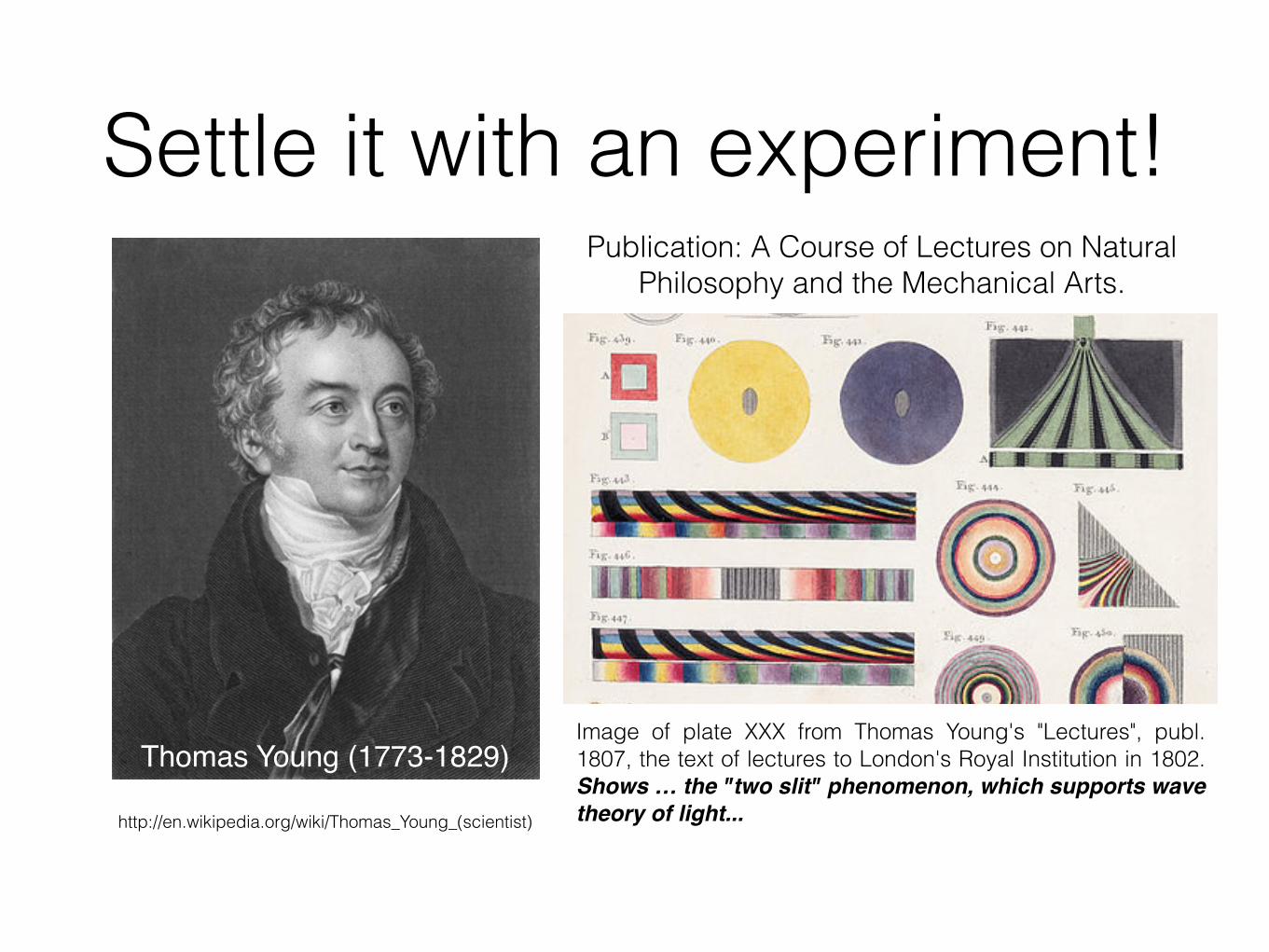
Publication: A Course of Lectures on Natural Philosophy and the Mechanical Arts.
Image of plate XXX from Thomas Young's "Lectures", publ. 1807, the text of lectures to London's Royal Institution in 1802. Shows … the "two slit" phenomenon, which supports wave theory of light...http://en.wikipedia.org/wiki/Thomas_Young_(scientist)
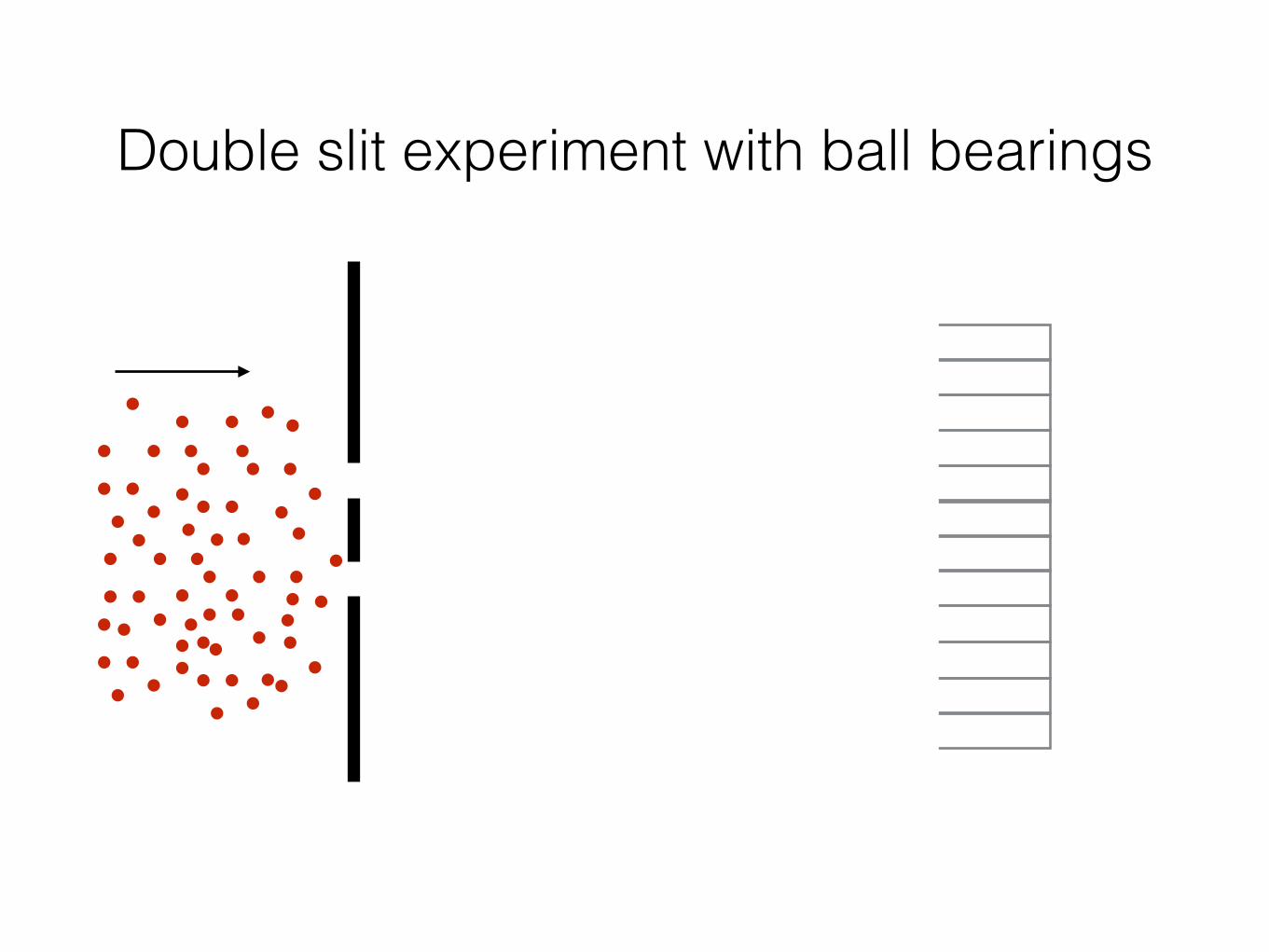
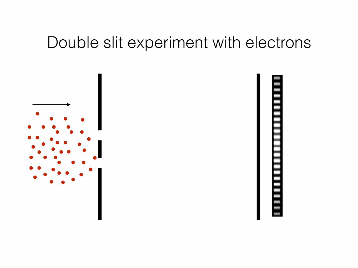
Double slit experiment with ball bearings
Double slit experiment with ball bearings
Double slit experiment with ball bearings
Double slit experiment with ball bearings
Double slit experiment with ball bearings
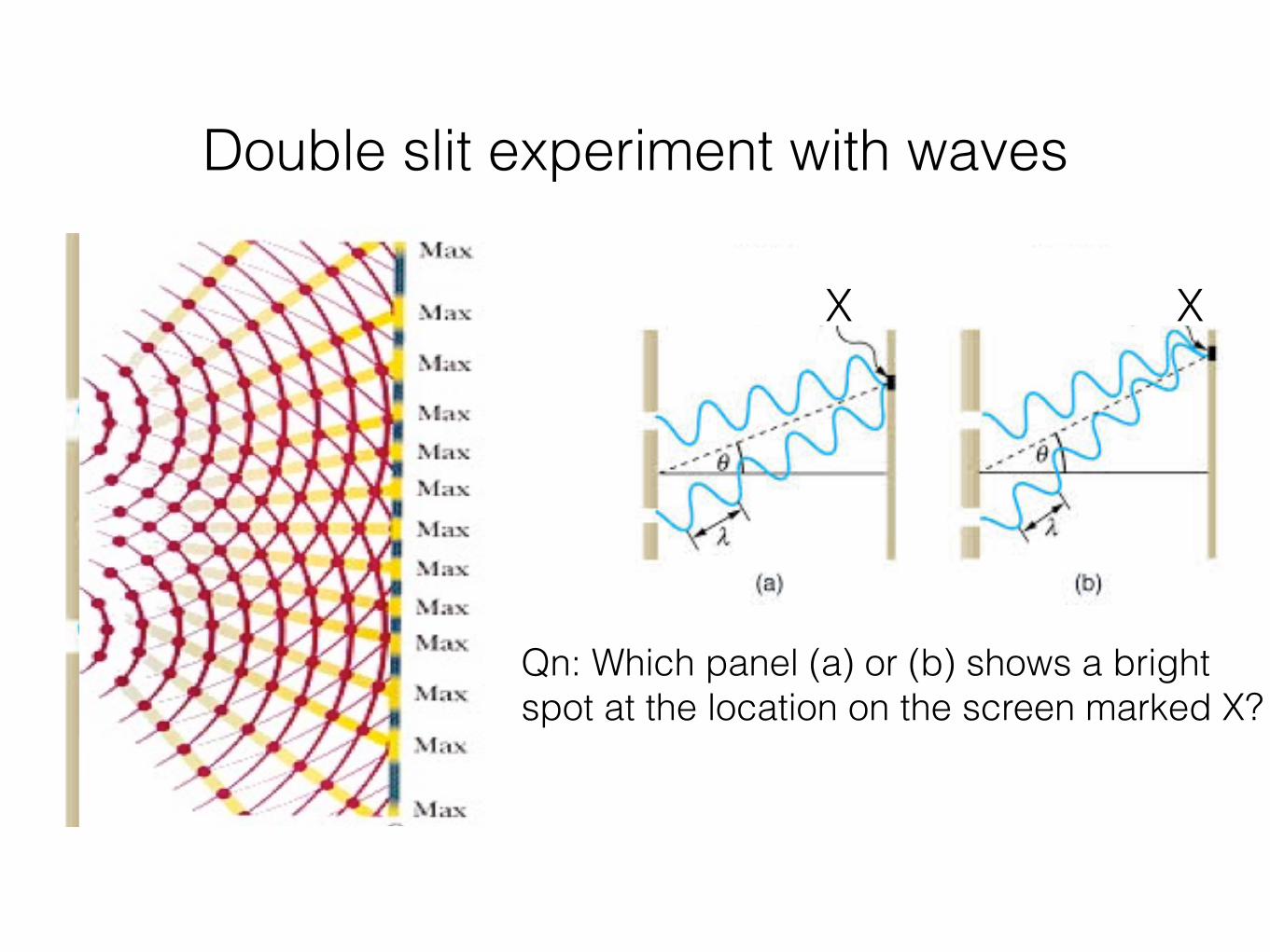
Qn: Which panel (a) or (b) shows a bright spot at the location on the screen marked X?
X X
Double slit experiment with waves
Young’s double slit experiment with light
https://www.youtube.com/watch?v=Iuv6hY6zsd0
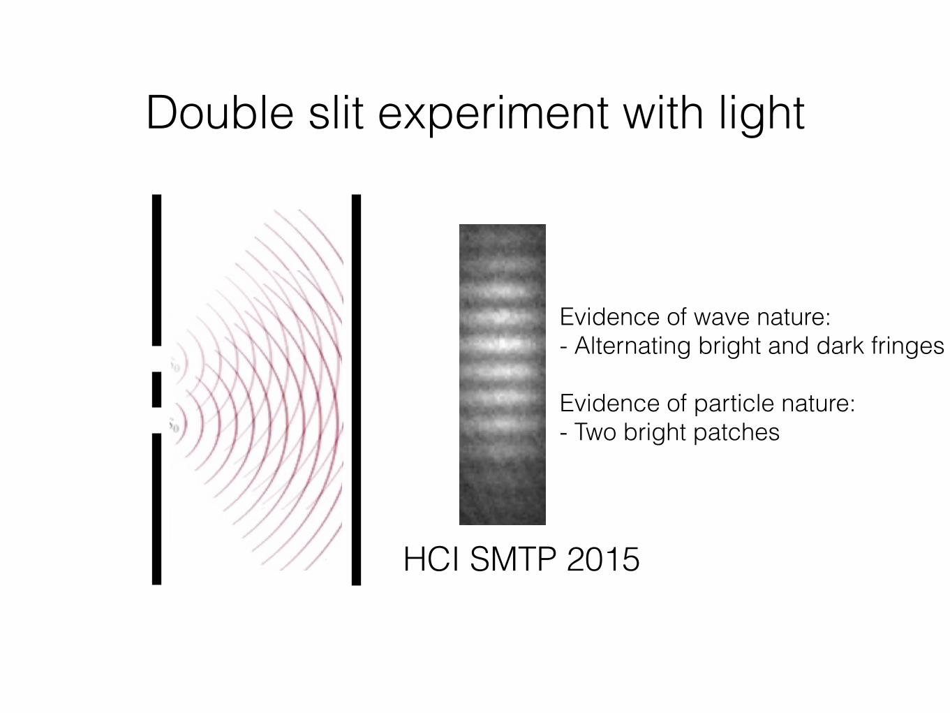
Double slit experiment with light
Evidence of wave nature: - Alternating bright and dark fringes
Evidence of particle nature: - Two bright patches
Double slit experiment with light
HCI SMTP 2015
Evidence of wave nature: - Alternating bright and dark fringes
Evidence of particle nature: - Two bright patches
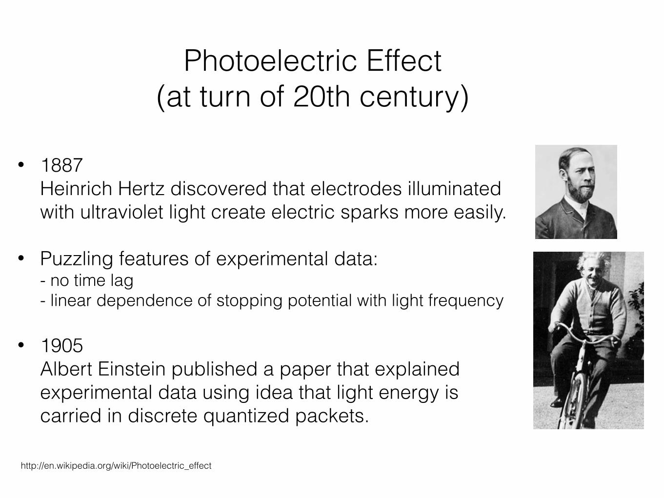
Photoelectric Effect (at turn of 20th century)
• 1887 Heinrich Hertz discovered that electrodes illuminated with ultraviolet light create electric sparks more easily.
• Puzzling features of experimental data: - no time lag- linear dependence of stopping potential with light frequency
• 1905 Albert Einstein published a paper that explained experimental data using idea that light energy is carried in discrete quantized packets.
http://en.wikipedia.org/wiki/Photoelectric_effect
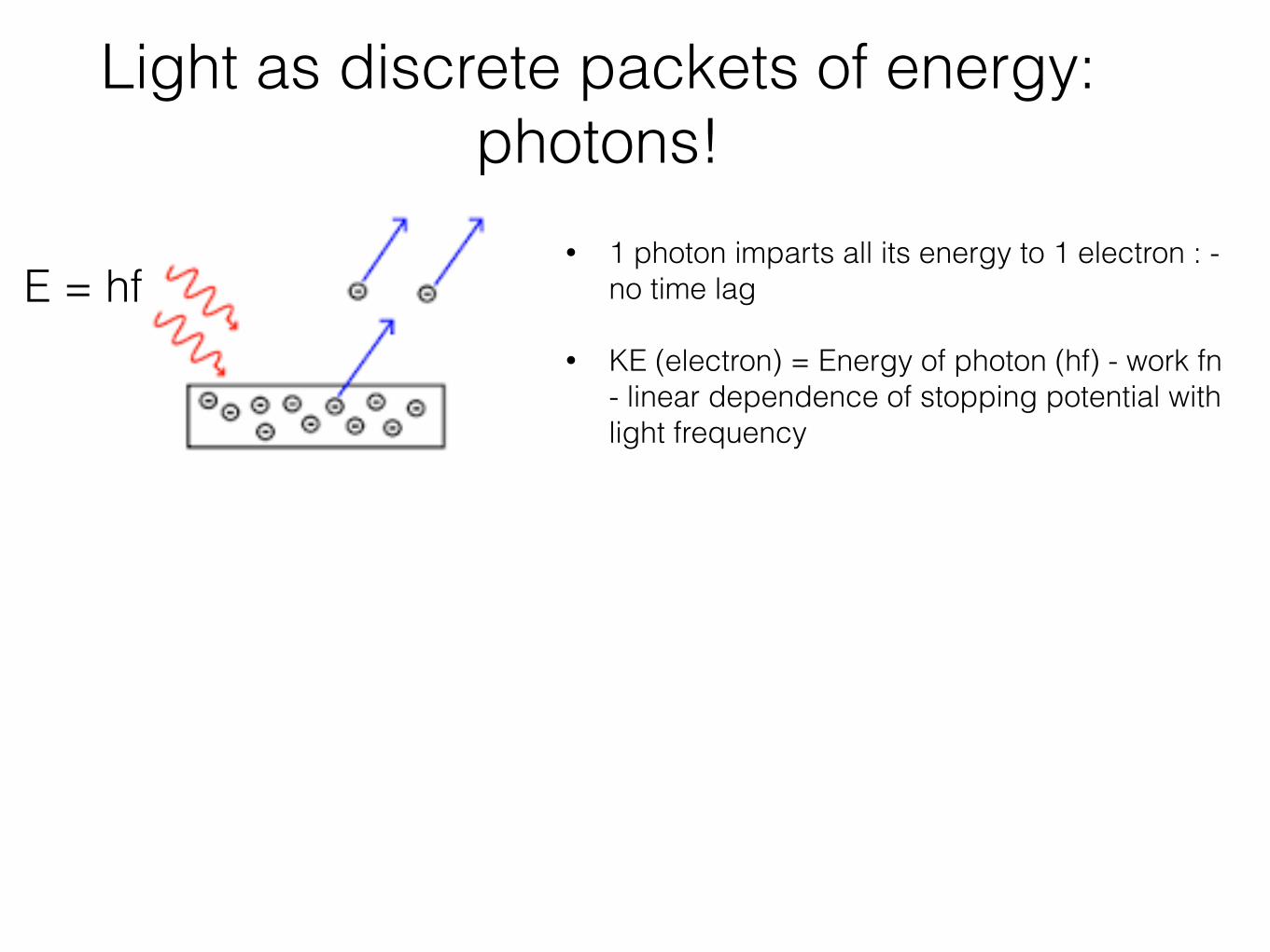
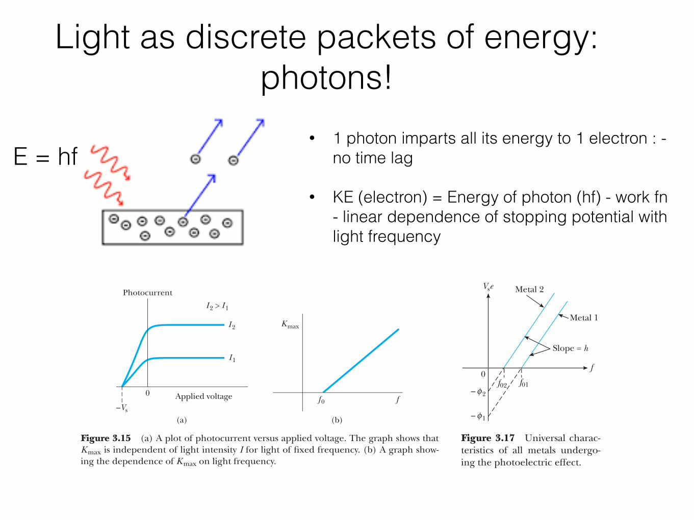
Light as discrete packets of energy: photons!
E = hf• 1 photon imparts all its energy to 1 electron : -
no time lag
• KE (electron) = Energy of photon (hf) - work fn - linear dependence of stopping potential with light frequency
Light as discrete packets of energy: photons!
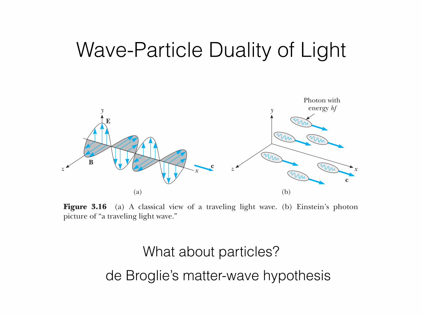
of the electron. In short, he introduced only those ideas necessary toexplain the photoelectric effect. He maintained that the energy of lightis not distributed evenly over the classical wavefront, but is concen-trated in discrete regions (or in “bundles”), called quanta, each con-taining energy, hf. A suggestive image, not to be taken too literally, isshown in Figure 3.16b. Einstein’s picture was that a light quantum was solocalized that it gave all its energy, hf, directly to a single electron in themetal. Therefore, according to Einstein, the maximum kinetic energy foremitted electrons is
(3.23)
where ! is the work function of the metal, which corresponds to the minimumenergy with which an electron is bound in the metal. Table 3.1 lists values ofwork functions measured for different metals.
Equation 3.23 beautifully explained the puzzling independence of Kmax
and intensity found by Lenard. For a fixed light frequency f, an increase inlight intensity means more photons and more photoelectrons per second,although Kmax remains unchanged according to Equation 3.23. In addition,Equation 3.23 explained the phenomenon of threshold frequency. Light ofthreshold frequency f0, which has just enough energy to knock an electron outof the metal surface, causes the electron to be released with zero kineticenergy. Setting Kmax " 0 in Equation 3.23 gives
(3.24)
Thus the variation in threshold frequency for different metals is producedby the variation in work function. Note that light with f # f0 has insuf-ficient energy to free an electron. Consequently, the photocurrent is zerofor f # f0.
With any theory, one looks not only for explanations of previously observedresults but also for new predictions. This was indeed the case here, as Equa-tion 3.23 predicted the result (new in 1905) that Kmax should vary linearlywith f for any material and that the slope of the Kmax versus f plot should yield
f0 "!
h
Kmax " hf $ !
84 CHAPTER 3 THE QUANTUM THEORY OF LIGHT
c
E
B
y
xz
(a) (b)
c
x
y
z
Photon withenergy hf
Figure 3.17 Universal charac-teristics of all metals undergo-ing the photoelectric effect.
Figure 3.16 (a) A classical view of a traveling light wave. (b) Einstein’s photonpicture of “a traveling light wave.”
Vse = hf –
Metal 2
Metal 1
Slope = h
f
f01f02
Vse
0
– 2
– 1
φ
φ
φ
Table 3.1 Work Functionsof SelectedMetals
Work Function, !,Metal (in eV)
Na 2.28Al 4.08Cu 4.70Zn 4.31Ag 4.73Pt 6.35Pb 4.14Fe 4.50
Einstein’s theory of thephotoelectric effect
Copyright 2005 Thomson Learning, Inc. All Rights Reserved.
was unable to establish the precise relationship, Lenard also indicated thatKmax increases with light frequency. A typical apparatus used to measure themaximum kinetic energy of photoelectrons is shown in Figure 3.14. Kmax iseasily measured by applying a retarding voltage and gradually increasing ituntil the most energetic electrons are stopped and the photocurrent becomeszero. At this point,
(3.21)
where me is the mass of the electron, vmax is the maximum electronspeed, e is the electronic charge, and Vs is the stopping voltage. A plotof the type found by Lenard is shown in Figure 3.15a; it illustrates thatK max or Vs is independent of light intensity I. The increase in current(or number of electrons per second) with increasing light intensityshown in Figure 3.15a was expected and could be explained classically.However, the result that K max does not depend on the intensity was completelyunexpected.
Two other experimental results were completely unexpected classically aswell. One was the linear dependence of Kmax on light frequency, shown in Figure3.15b. Note that Figure 3.15b also shows the existence of a thresholdfrequency, f0, below which no photoelectrons are emitted. (Actually, athreshold energy called the work function, !, is associated with the bindingenergy of an electron in a metal and is expected classically. That there is anenergy barrier holding electrons in a solid is evident from the fact thatelectrons are not spontaneously emitted from a metal in a vacuum, butrequire high temperatures or incident light to provide an energy of !and cause emission.) The other interesting result impossible to explainclassically is that there is no time lag between the start of illumination andthe start of the photocurrent. Measurements have shown that if there isa time lag, it is less than 10"9 s. In summary, as shown in detail in thefollowing example, classical electromagnetic theory has major difficul-ties explaining the independence of K max and light intensity, the lineardependence of K max on light frequency, and the instantaneous responseof the photocurrent.
Kmax # 12mev2
max # eVs
82 CHAPTER 3 THE QUANTUM THEORY OF LIGHT
0 Applied voltage
(a)
Photocurrent
I2 > I1
I2
I1
–Vs
(b)
Kmax
f0 f
Figure 3.15 (a) A plot of photocurrent versus applied voltage. The graph shows thatKmax is independent of light intensity I for light of fixed frequency. (b) A graph show-ing the dependence of Kmax on light frequency.
Figure 3.14 Photoelectric ef-fect apparatus.
Metallicemitter
Collector
Light
Sensitiveammeter
10-V supply
+ –
–
A
V
Copyright 2005 Thomson Learning, Inc. All Rights Reserved.
E = hf• 1 photon imparts all its energy to 1 electron : -
no time lag
• KE (electron) = Energy of photon (hf) - work fn - linear dependence of stopping potential with light frequency
of the electron. In short, he introduced only those ideas necessary toexplain the photoelectric effect. He maintained that the energy of lightis not distributed evenly over the classical wavefront, but is concen-trated in discrete regions (or in “bundles”), called quanta, each con-taining energy, hf. A suggestive image, not to be taken too literally, isshown in Figure 3.16b. Einstein’s picture was that a light quantum was solocalized that it gave all its energy, hf, directly to a single electron in themetal. Therefore, according to Einstein, the maximum kinetic energy foremitted electrons is
(3.23)
where ! is the work function of the metal, which corresponds to the minimumenergy with which an electron is bound in the metal. Table 3.1 lists values ofwork functions measured for different metals.
Equation 3.23 beautifully explained the puzzling independence of Kmax
and intensity found by Lenard. For a fixed light frequency f, an increase inlight intensity means more photons and more photoelectrons per second,although Kmax remains unchanged according to Equation 3.23. In addition,Equation 3.23 explained the phenomenon of threshold frequency. Light ofthreshold frequency f0, which has just enough energy to knock an electron outof the metal surface, causes the electron to be released with zero kineticenergy. Setting Kmax " 0 in Equation 3.23 gives
(3.24)
Thus the variation in threshold frequency for different metals is producedby the variation in work function. Note that light with f # f0 has insuf-ficient energy to free an electron. Consequently, the photocurrent is zerofor f # f0.
With any theory, one looks not only for explanations of previously observedresults but also for new predictions. This was indeed the case here, as Equa-tion 3.23 predicted the result (new in 1905) that Kmax should vary linearlywith f for any material and that the slope of the Kmax versus f plot should yield
f0 "!
h
Kmax " hf $ !
84 CHAPTER 3 THE QUANTUM THEORY OF LIGHT
c
E
B
y
xz
(a) (b)
c
x
y
z
Photon withenergy hf
Figure 3.17 Universal charac-teristics of all metals undergo-ing the photoelectric effect.
Figure 3.16 (a) A classical view of a traveling light wave. (b) Einstein’s photonpicture of “a traveling light wave.”
Vse = hf –
Metal 2
Metal 1
Slope = h
f
f01f02
Vse
0
– 2
– 1
φ
φ
φ
Table 3.1 Work Functionsof SelectedMetals
Work Function, !,Metal (in eV)
Na 2.28Al 4.08Cu 4.70Zn 4.31Ag 4.73Pt 6.35Pb 4.14Fe 4.50
Einstein’s theory of thephotoelectric effect
Copyright 2005 Thomson Learning, Inc. All Rights Reserved.
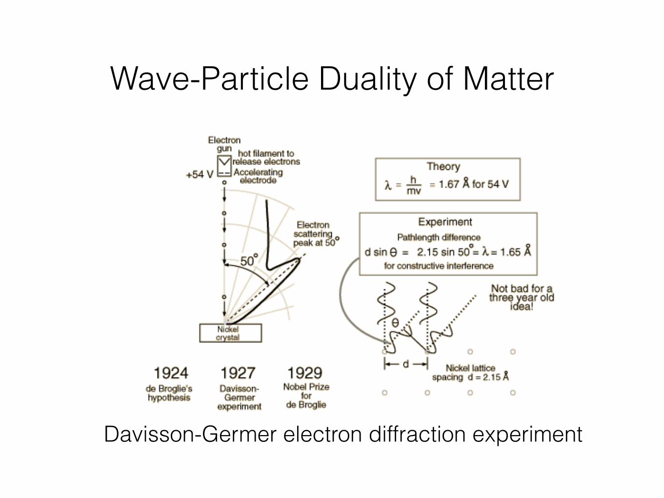
What about particles?de Broglie’s matter-wave hypothesis
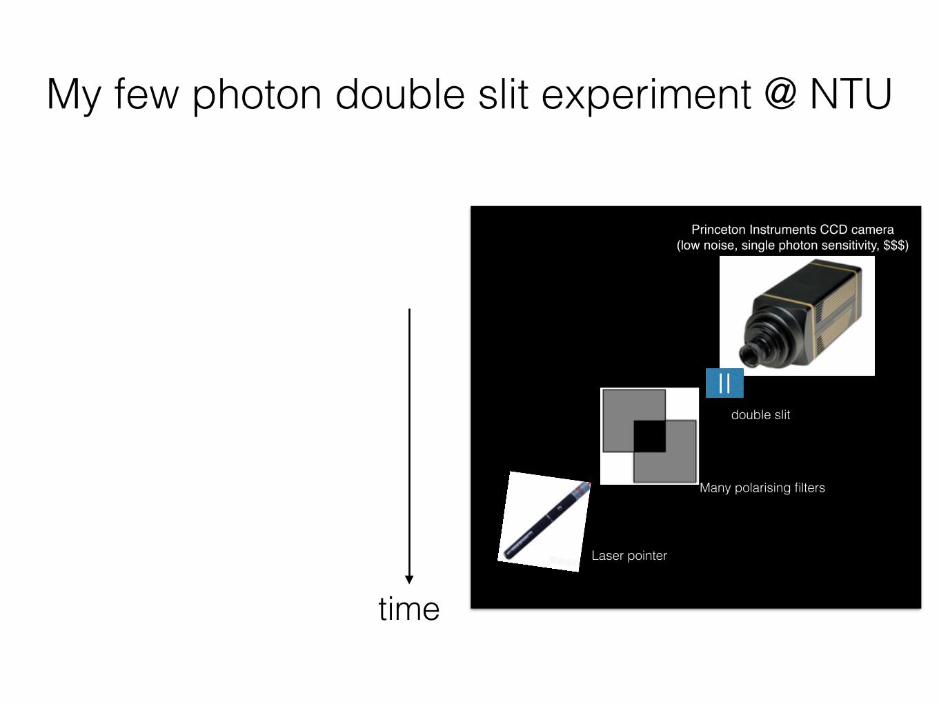
Princeton Instruments CCD camera (low noise, single photon sensitivity, $$$)
IIdouble slit
My few photon double slit experiment @ NTU
time
Laser pointer
Many polarising filters
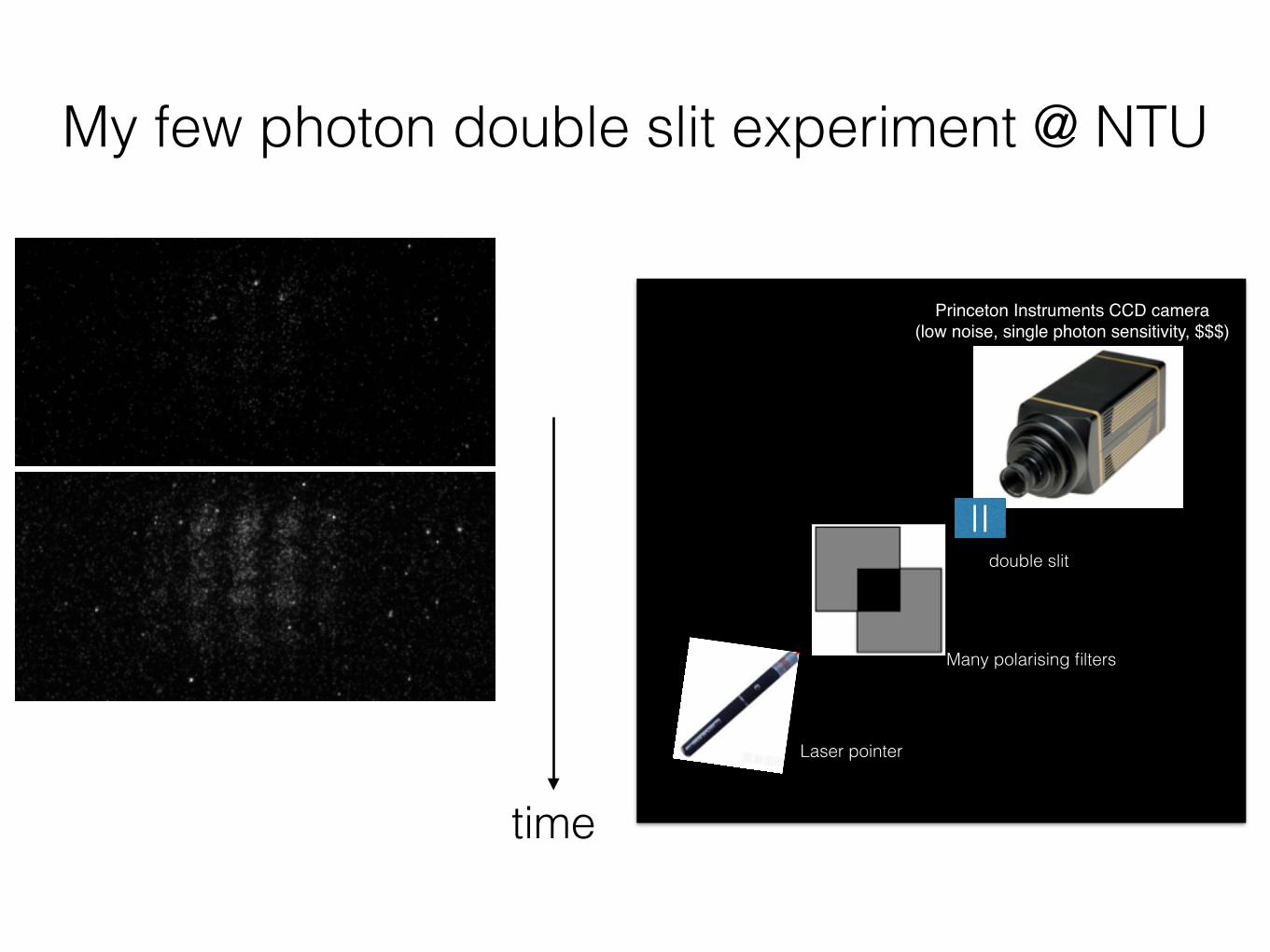
Princeton Instruments CCD camera (low noise, single photon sensitivity, $$$)
IIdouble slit
My few photon double slit experiment @ NTU
time
Laser pointer
Many polarising filters
Princeton Instruments CCD camera (low noise, single photon sensitivity, $$$)
IIdouble slit
My few photon double slit experiment @ NTU
time
Laser pointer
Many polarising filters
Princeton Instruments CCD camera (low noise, single photon sensitivity, $$$)
IIdouble slit
My few photon double slit experiment @ NTU
time
Laser pointer
Many polarising filters
Princeton Instruments CCD camera (low noise, single photon sensitivity, $$$)
IIdouble slit
Classical intuition about the electron
Hmm… the electron must have gone through one or the other slit.
Which slit did the electron pass through?
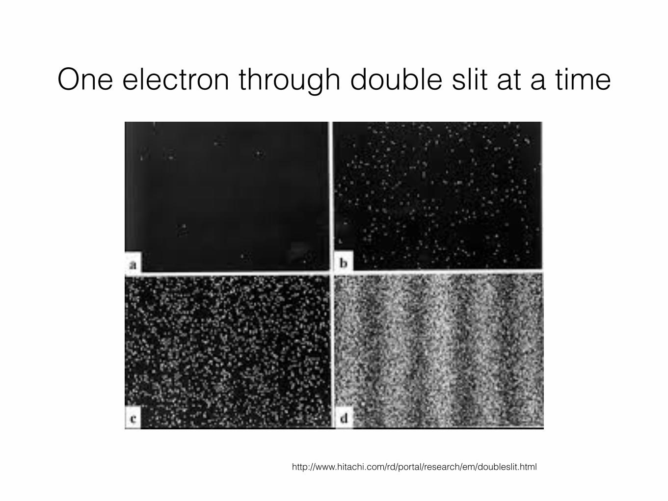
both slits open. Note in Figure 5.31 that there is no longer a maximumprobability of arrival of an electron at ! " 0. In fact, the interferencepattern has been lost and the accumulated result is simply the sum ofthe individual results. The results shown by the black curves in Figure5.31 are easier to understand and more reasonable than the interference ef-fects seen with both slits open (blue curve). When only one slit is open at atime, we know the electron has the same localizability and indivisibility atthe slits as we measure at the detector, because the electron clearly goesthrough slit 1 or slit 2. Thus, the total must be analyzed as the sum of thoseelectrons that come through slit 1, !#1 !2, and those that come through slit2, !#2 !2. When both slits are open, it is tempting to assume that the electrongoes through either slit 1 or slit 2 and that the counts per minute are againgiven by !#1 !2 $ !#2 !2. We know, however, that the experimental resultscontradict this. Thus, our assumption that the electron is localized and goesthrough only one slit when both slits are open must be wrong (a painfulconclusion!). Somehow the electron must be simultaneously present at bothslits in order to exhibit interference.
To find the probability of detecting the electron at a particular point on thescreen with both slits open, we may say that the electron is in a superpositionstate given by
# " #1 $ #2
182 CHAPTER 5 MATTER WAVES
2
1
2
1
counts/min
⏐ 2⏐2Ψ
⏐ 1⏐2Ψ
Figure 5.30 The probability of finding electrons at the screen with either the loweror upper slit closed.
Copyright 2005 Thomson Learning, Inc. All Rights Reserved.
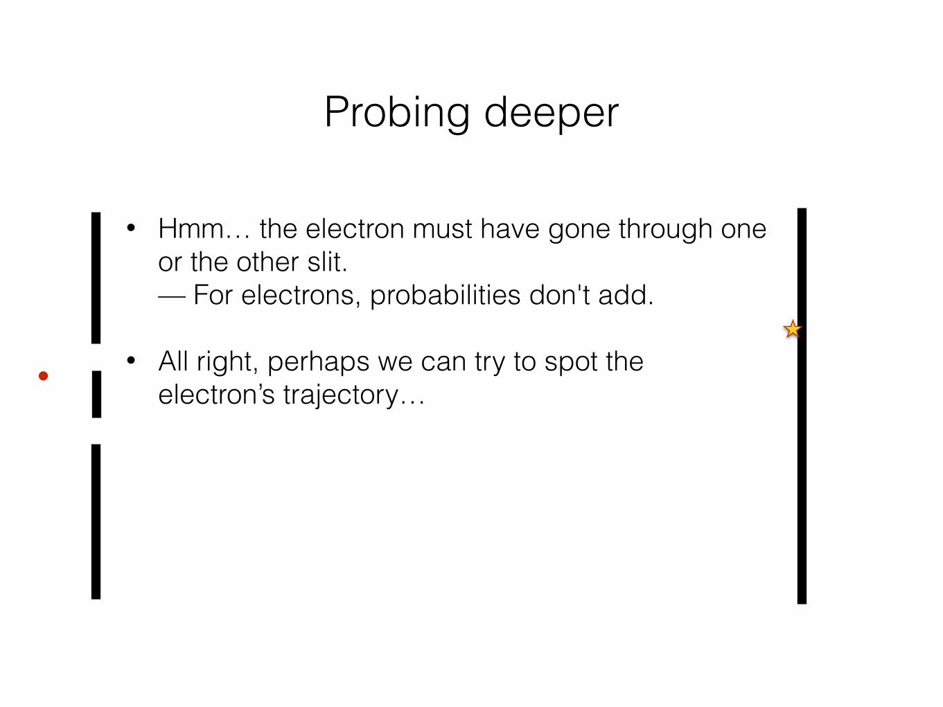
Probing deeper
• Hmm… the electron must have gone through one or the other slit. — For electrons, probabilities don't add.
• All right, perhaps we can try to spot the electron’s trajectory…
Watching the electron
light source
Watching the electron
light source
Watching the electron
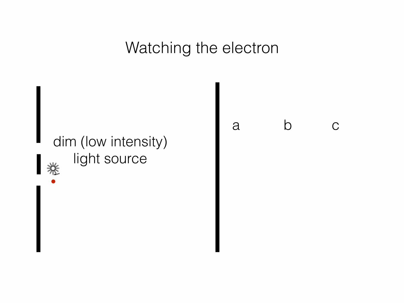
dim (low intensity) light source
a b c
Watching the electron
dim (low intensity) light source
a b c
Watching the electron
dim (low intensity) light source
a b c
Qn: Order the 3 patterns in decreasing intensity of light.
Watching the electron …
certainty principle. We consider certain idealized experiments (called thought ex-periments) and show that it is impossible to carry out an experiment that allowsthe position and momentum of a particle to be simultaneously measured with anaccuracy that violates the uncertainty principle. The most famous thought experi-ment along these lines was introduced by Heisenberg himself and involves themeasurement of an electron’s position by means of a microscope (Fig. 5.26),which forms an image of the electron on a screen or the retina of the eye.
Because light can scatter from and perturb the electron, let us minimizethis effect by considering the scattering of only a single light quantum from anelectron initially at rest (Fig. 5.27). To be collected by the lens, thephoton must be scattered through an angle ranging from !" to #", whichconsequently imparts to the electron an x momentum value ranging from#(h sin ")/$ to !(h sin")/$. Thus the uncertainty in the electron’s momen-tum is %px & (2h sin")/$. After passing through the lens, the photon landssomewhere on the screen, but the image and consequently the position of theelectron is “fuzzy” because the photon is diffracted on passing through thelens aperture. According to physical optics, the resolution of a microscope orthe uncertainty in the image of the electron, %x, is given by %x & $/(2 sin ").Here 2" is the angle subtended by the objective lens, as shown in Figure 5.27.5
Multiplying the expressions for %px and %x, we find for the electron
176 CHAPTER 5 MATTER WAVES
Figure 5.27 The Heisenberg microscope.
Figure 5.26 A thought experi-ment for viewing an electronwith a powerful microscope.(a) The electron is shown be-fore colliding with the photon.(b) The electron recoils (is dis-turbed) as a result of the colli-sion with the photon.
5The resolving power of the microscope is treated clearly in F. A. Jenkins and H. E. White, Funda-mentals of Optics, 4th ed., New York, McGraw-Hill Book Co., 1976, pp. 332–334.
Incidentphoton
Beforecollision
Electron
(a)
Scatteredphoton
Aftercollision
Recoilingelectron
(b)
x
y
Lens
Scattered photonp = h/λ
λ
e – initiallyat rest
Incident photonp0 = h/ 0
∆x
∆x
θα
Screen
Copyright 2005 Thomson Learning, Inc. All Rights Reserved.
Is there not some way we can see the electrons without disturbing them?
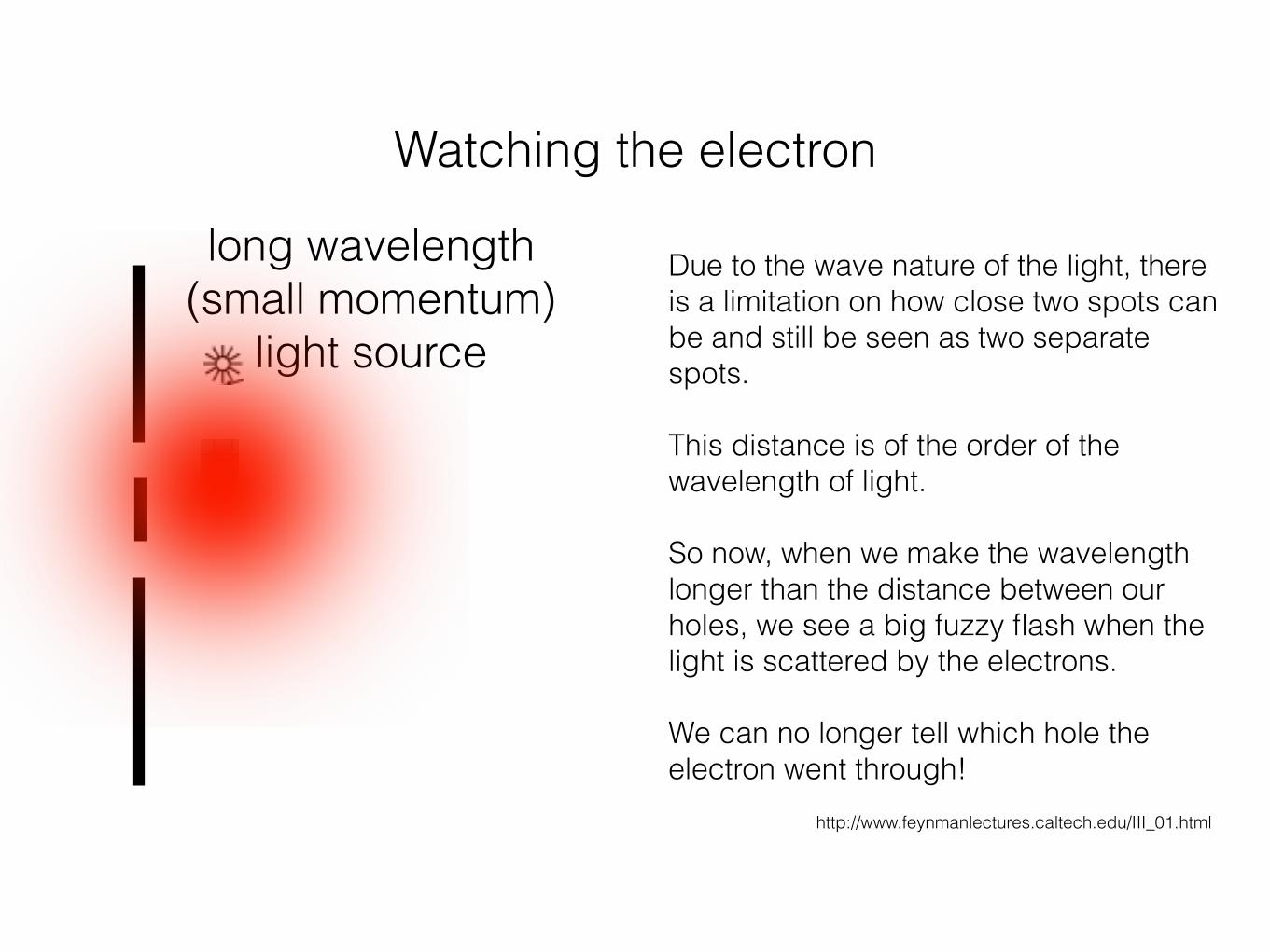
Watching the electron
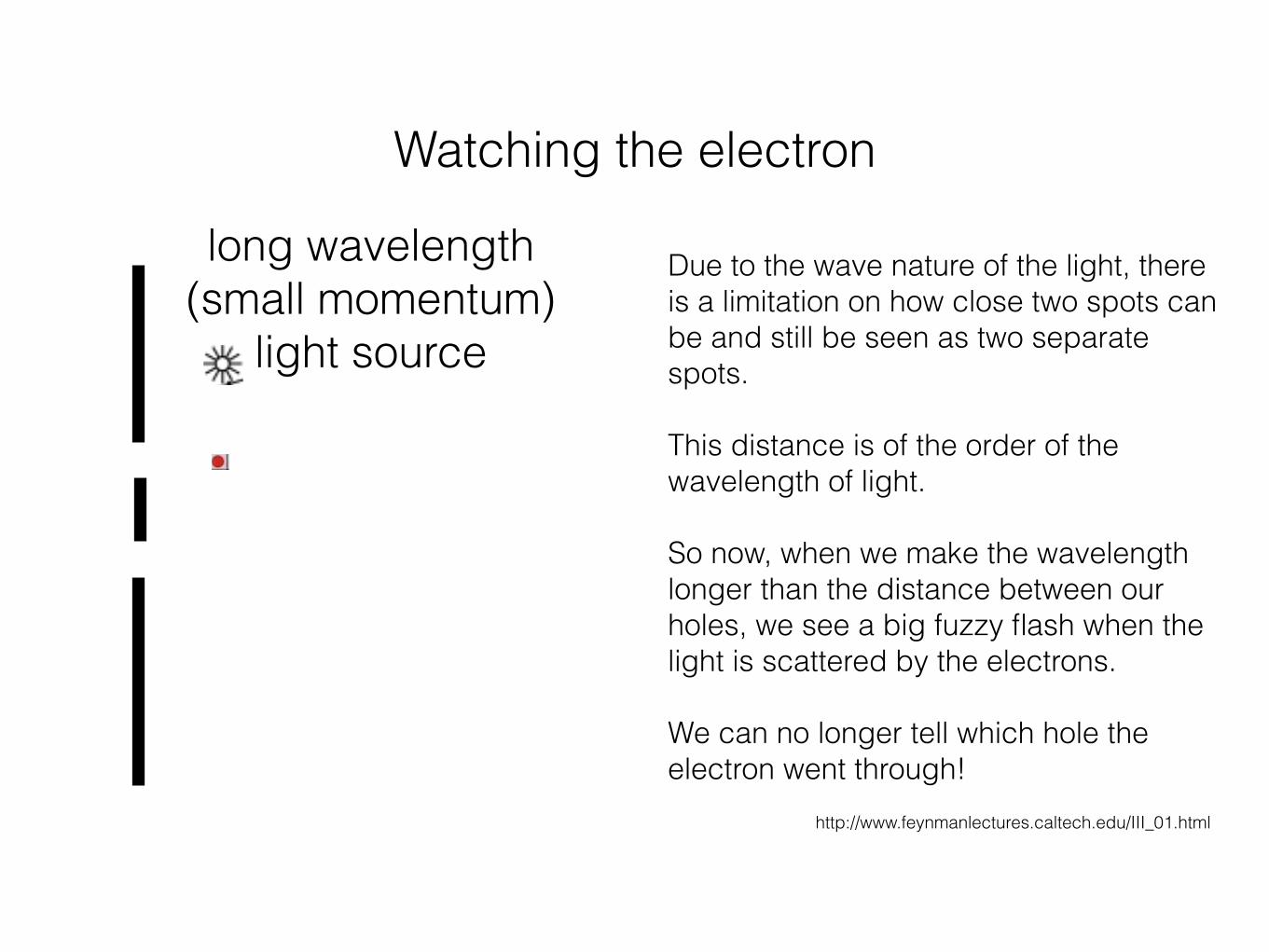
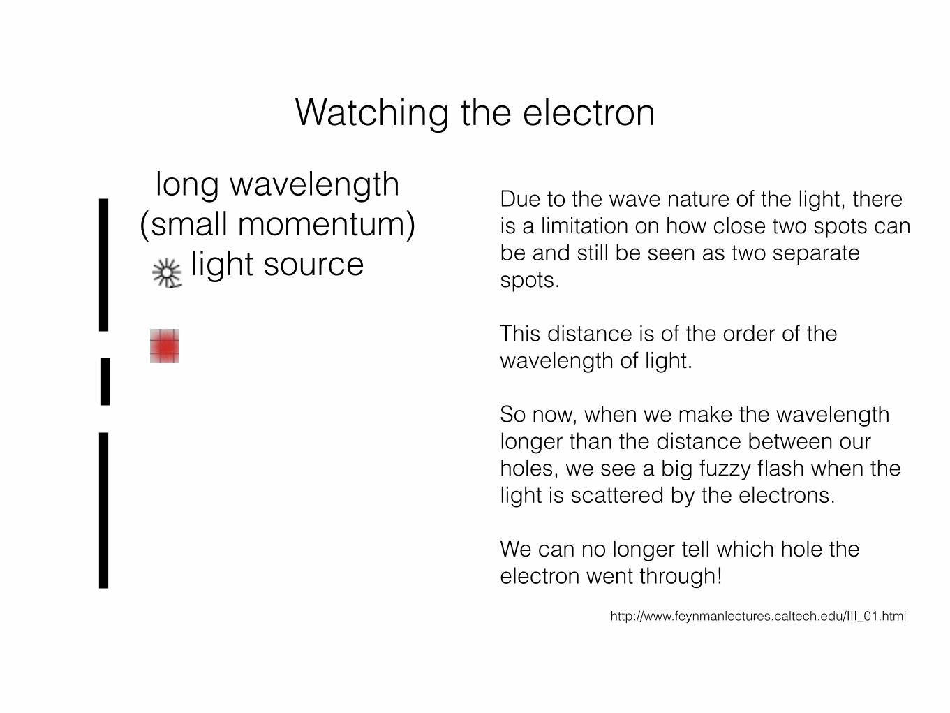
long wavelength (small momentum)
light source
Due to the wave nature of the light, there is a limitation on how close two spots can be and still be seen as two separate spots.
This distance is of the order of the wavelength of light.
So now, when we make the wavelength longer than the distance between our holes, we see a big fuzzy flash when the light is scattered by the electrons.
We can no longer tell which hole the electron went through!
Qn: Order the 3 patterns in increasing wavelength of light.
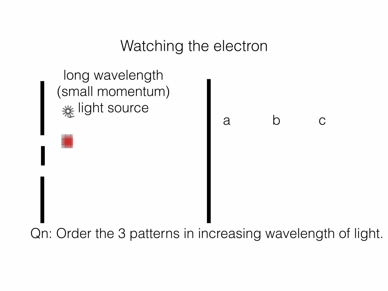
Watching the electron
long wavelength (small momentum)
light source a b c
Qn: Order the 3 patterns in increasing wavelength of light.
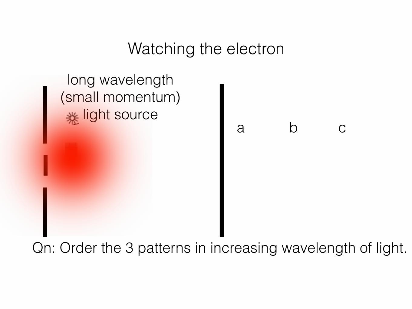
Watching the electron
long wavelength (small momentum)
light source a b c
Qn: Order the 3 patterns in increasing wavelength of light.
Watching the electron
long wavelength (small momentum)
light source a b c
Qn: Order the 3 patterns in increasing wavelength of light.
Heisenberg Uncertainty Principle
“It is impossible to design an apparatus to determine which hole the electron passes through, that will not at the same time disturb the electrons enough to destroy the
interference pattern.”
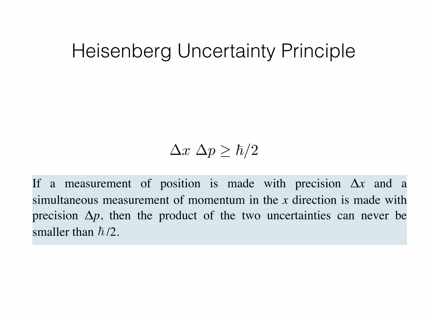
Heisenberg Uncertainty Principle
�x �p � �/2
If a measurement of position is made with precision Δx and a simultaneous measurement of momentum in the x direction is made with precision Δp, then the product of the two uncertainties can never be smaller than /2. �
Heisenberg Uncertainty Principle
�x �p � �/2
If a measurement of position is made with precision Δx and a simultaneous measurement of momentum in the x direction is made with precision Δp, then the product of the two uncertainties can never be smaller than /2. �
Position x, and momentum p, are incompatible observables
What have we learnt so far? (1)
age14 15 16 17 18 19 20 21 22
11
8
P(age=19) = 10% N
What have we learnt so far? (1)• We describe the quantum world in terms of probability
age14 15 16 17 18 19 20 21 22
11
8
P(age=19) = 10% N
wavefunction-squared (probability density)
What have we learnt so far? (1)• We describe the quantum world in terms of probability
age14 15 16 17 18 19 20 21 22
11
8
P(age=19) = 10% N
wavefunction-squared (probability density)
Statistical Interpretation of QM
Even if you know everything the theory has to tell you about the particle, you cannot predict with certainty, the outcome of a simple experiment to measure its position.
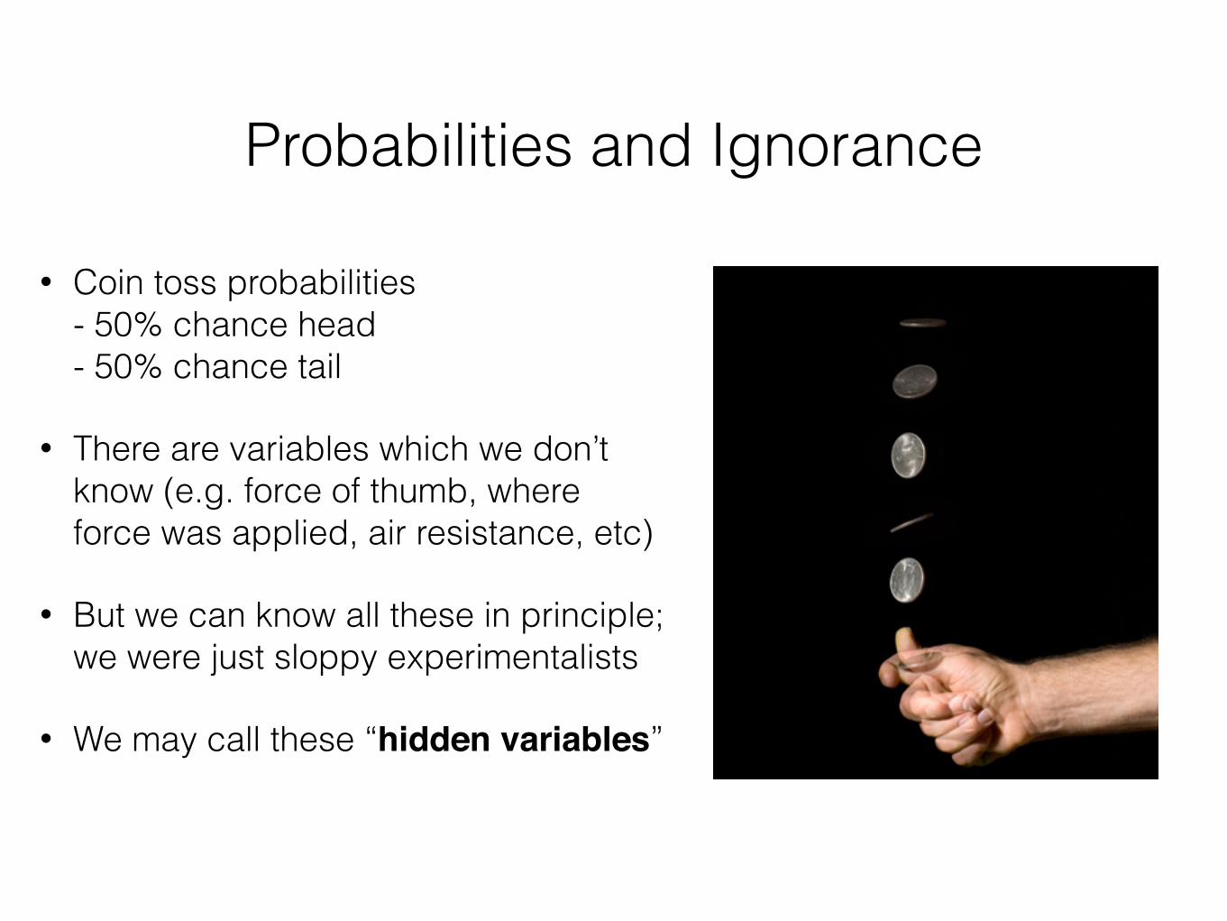
• There are variables which we don’t know (e.g. force of thumb, where force was applied, air resistance, etc)
• But we can know all these in principle; we were just sloppy experimentalists
• We may call these “hidden variables”
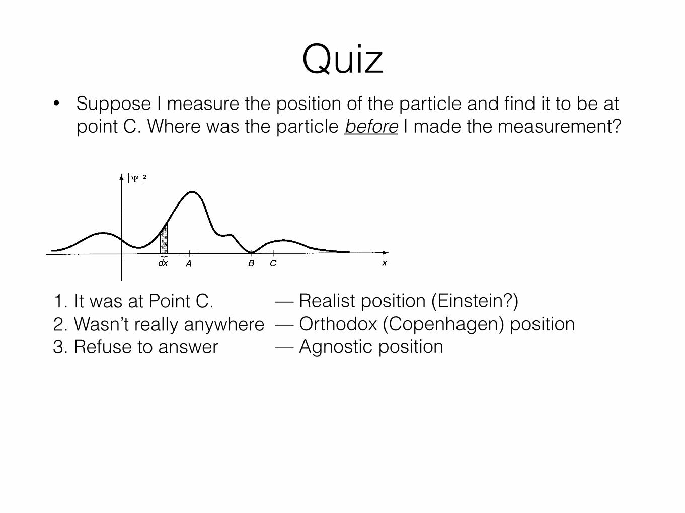
Quiz• Suppose I measure the position of the particle and find it to be at
point C. Where was the particle before I made the measurement?
1. It was at Point C. 2. Wasn’t really anywhere 3. Refuse to answer
Quiz• Suppose I measure the position of the particle and find it to be at
point C. Where was the particle before I made the measurement?
1. It was at Point C. 2. Wasn’t really anywhere 3. Refuse to answer
— Realist position (Einstein?) — Orthodox (Copenhagen) position — Agnostic position
Quiz• Suppose I measure the position of the particle and find it to be at
point C. Where was the particle before I made the measurement?
1. It was at Point C. 2. Wasn’t really anywhere 3. Refuse to answer
— Realist position (Einstein?) — Orthodox (Copenhagen) position — Agnostic position
1
PHYSICS TODAY / APRIL 1985 PAG. 38-47
Is the moon there when nobody looks?Reality and the quantum theory
Einstein maintained that quantum metaphysics entails spooky actions at a distance;experiments have now shown that what bothered Einstein is not a debatable pointbut the observed behaviour of the real world.
N. David Mermin
[David Mermin is director of the Laboratory of Atomic and Solid State Physics at Cornell University. A
solid-state theorist, he has recently come up with some quasithoughts about quasicrystals. He is known to
PHYSICS TODAY readers as the person who made “boojum” an internationally accepted scientific term.
With N.W.Ashcroft, he is about to start updating the world’s funniest solid-state physics text.
He says he is bothered by Bell’s theorem, but may have rocks in his head anyway.]
Quantum mechanics is magic1
In May 1935, Albert Einstein, Boris Podolsky and Nathan Rosen published2 an argument that quantum
mechanics fails to provide a complete description of physical reality. Today, 50 years later, the EPR paper
and the theoretical and experimental work it inspired remain remarkable for the vivid illustration they
provide of one of the most bizarre aspects of the world revealed to us by the quantum theory.
Einstein’s talent for saying memorable things did him a disservice when he declared “God does not play
dice.” for it has been held ever since the basis for his opposition to quantum mechanics was the claim that a
fundamental understanding of the world can only be statistical.
But the EPR paper, his most powerful attack on the quantum theory, focuses on quite a different aspect: the
doctrine that physical properties have in general no objective reality independent of the act of observation.
As Pascual Jordan put it3:
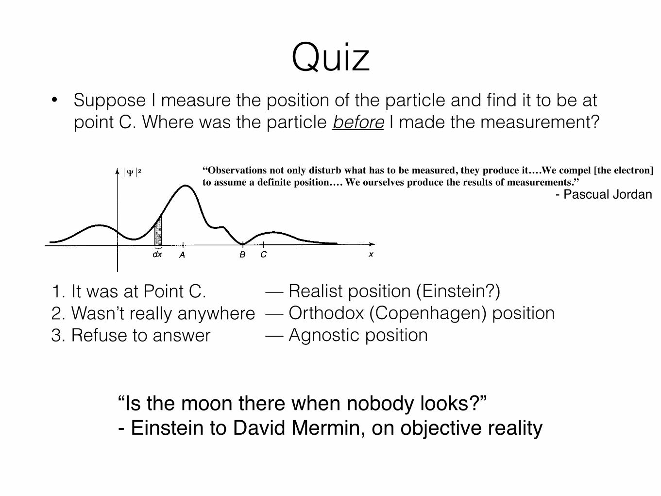
“Observations not only disturb what has to be measured, they produce it….We compel [the electron]
to assume a definite position…. We ourselves produce the results of measurements.”
Jordan’s statement is something of a truism for contemporary physicists. Underlying it, we have all been
taught, is the disruption of what is being measured by the act of measurement, made unavoidable by the
existence of the quantum of action, which generally makes it impossible even in principle to construct probes
that can yield the information classical intuition expects to be there.
Einstein didn’t like this. He wanted things out there to have properties, whether or not they were measured4:
“We often discussed his notions on objective reality. I recall that during one walk Einstein suddenly
stopped, turned to me and asked whether I really believed that the moon exists only when I look at it.”
The EPR paper describes a situation ingeniously contrived to force the quantum theory into asserting that
properties in a space-time region B are the result of an act of measurement in another space-time region A,
so far from B that there is no possibility of the measurement in A exerting an influence on region B by any
known dynamical mechanism. Under these conditions, Einstein maintained that the properties in A must
have existed all along.
- Pascual Jordan
Quiz• Suppose I measure the position of the particle and find it to be at
point C. Where was the particle before I made the measurement?
1. It was at Point C. 2. Wasn’t really anywhere 3. Refuse to answer
— Realist position (Einstein?) — Orthodox (Copenhagen) position — Agnostic position
“Is the moon there when nobody looks?” - Einstein to David Mermin, on objective reality
1
PHYSICS TODAY / APRIL 1985 PAG. 38-47
Is the moon there when nobody looks?Reality and the quantum theory
Einstein maintained that quantum metaphysics entails spooky actions at a distance;experiments have now shown that what bothered Einstein is not a debatable pointbut the observed behaviour of the real world.
N. David Mermin
[David Mermin is director of the Laboratory of Atomic and Solid State Physics at Cornell University. A
solid-state theorist, he has recently come up with some quasithoughts about quasicrystals. He is known to
PHYSICS TODAY readers as the person who made “boojum” an internationally accepted scientific term.
With N.W.Ashcroft, he is about to start updating the world’s funniest solid-state physics text.
He says he is bothered by Bell’s theorem, but may have rocks in his head anyway.]
Quantum mechanics is magic1
In May 1935, Albert Einstein, Boris Podolsky and Nathan Rosen published2 an argument that quantum
mechanics fails to provide a complete description of physical reality. Today, 50 years later, the EPR paper
and the theoretical and experimental work it inspired remain remarkable for the vivid illustration they
provide of one of the most bizarre aspects of the world revealed to us by the quantum theory.
Einstein’s talent for saying memorable things did him a disservice when he declared “God does not play
dice.” for it has been held ever since the basis for his opposition to quantum mechanics was the claim that a
fundamental understanding of the world can only be statistical.
But the EPR paper, his most powerful attack on the quantum theory, focuses on quite a different aspect: the
doctrine that physical properties have in general no objective reality independent of the act of observation.
As Pascual Jordan put it3:
“Observations not only disturb what has to be measured, they produce it….We compel [the electron]
to assume a definite position…. We ourselves produce the results of measurements.”
Jordan’s statement is something of a truism for contemporary physicists. Underlying it, we have all been
taught, is the disruption of what is being measured by the act of measurement, made unavoidable by the
existence of the quantum of action, which generally makes it impossible even in principle to construct probes
that can yield the information classical intuition expects to be there.
Einstein didn’t like this. He wanted things out there to have properties, whether or not they were measured4:
“We often discussed his notions on objective reality. I recall that during one walk Einstein suddenly
stopped, turned to me and asked whether I really believed that the moon exists only when I look at it.”
The EPR paper describes a situation ingeniously contrived to force the quantum theory into asserting that
properties in a space-time region B are the result of an act of measurement in another space-time region A,
so far from B that there is no possibility of the measurement in A exerting an influence on region B by any
known dynamical mechanism. Under these conditions, Einstein maintained that the properties in A must
have existed all along.
- Pascual Jordan
Schrodinger’s Cat
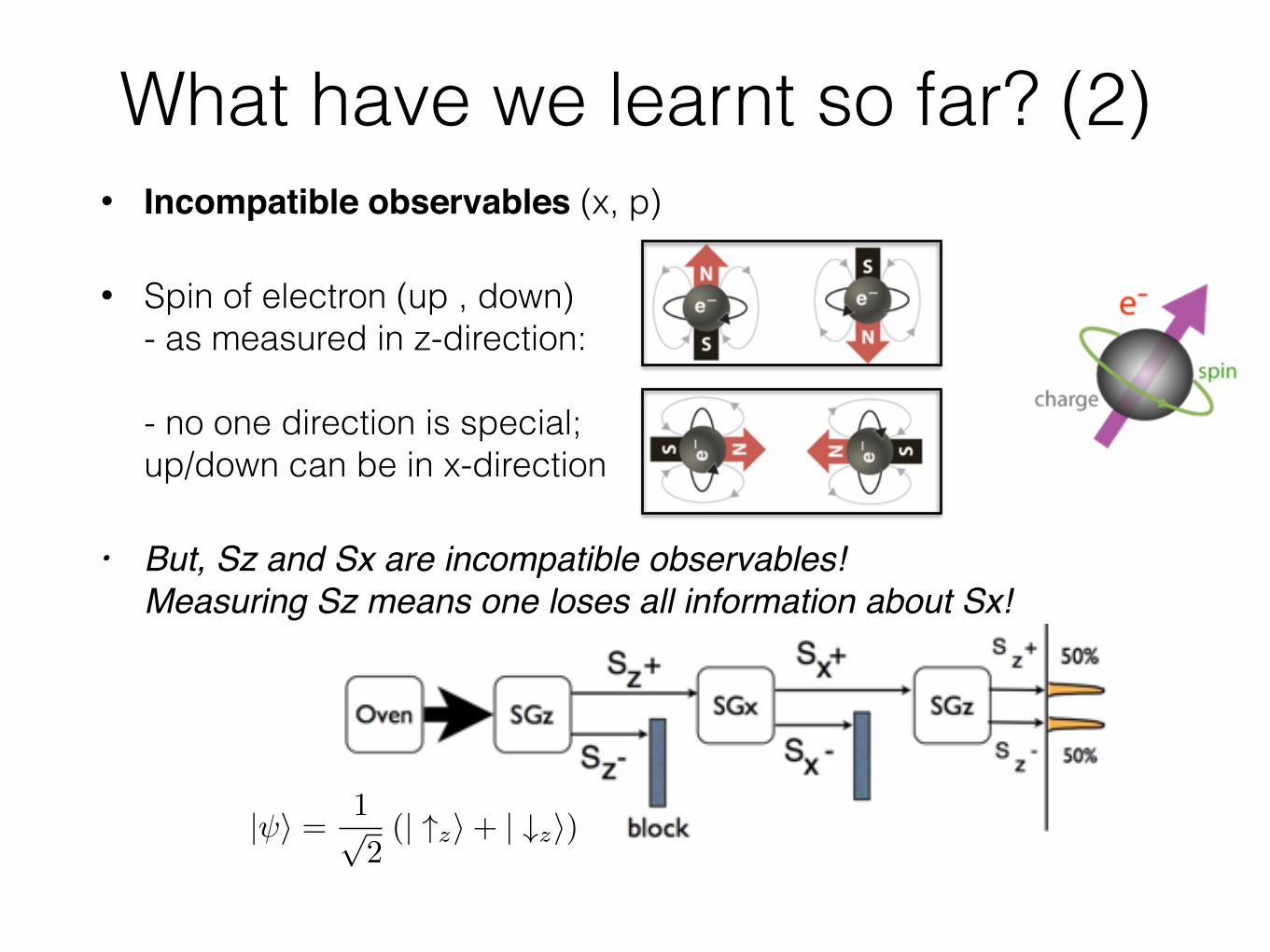
• Incompatible observables (x, p)
• Spin of electron (up , down) - as measured in z-direction: - no one direction is special; up/down can be in x-direction
• But, Sz and Sx are incompatible observables!Measuring Sz means one loses all information about Sx!
What have we learnt so far? (2)
• Incompatible observables (x, p)
• Spin of electron (up , down) - as measured in z-direction: - no one direction is special; up/down can be in x-direction
• But, Sz and Sx are incompatible observables!Measuring Sz means one loses all information about Sx!
What have we learnt so far? (2)
|�� =1�2
(| �z� + | �z�)
Entanglement
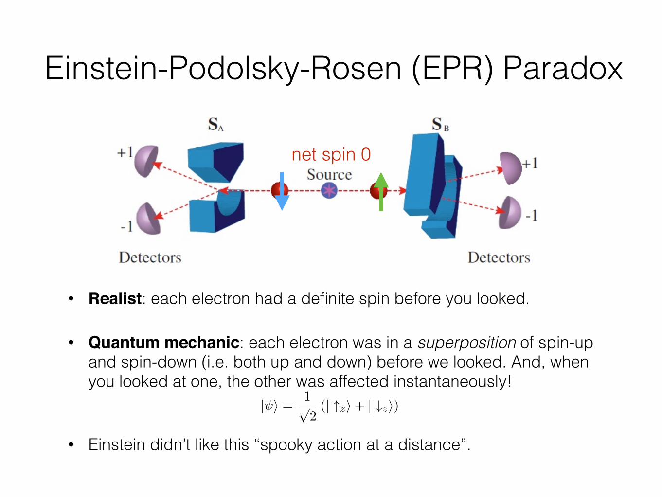
net spin 0
• Source has net spin = 0, net momentum = 0
• Source emits a pair of electrons; sum of electrons’ spins = 0 and they move in opposite directions
• Detect the spin state of electrons:Suppose z-direction chosen: whenever one is detected spin-up, the other is found to be spin-down and vice-versa.
Einstein-Podolsky-Rosen (EPR) Paradox
net spin 0
• Realist: each electron had a definite spin before you looked.
• Quantum mechanic: each electron was in a superposition of spin-up and spin-down (i.e. both up and down) before we looked. And, when you looked at one, the other was affected instantaneously!
• Einstein didn’t like this “spooky action at a distance”.
|�� =1�2
(| �z� + | �z�)
Einstein-Podolsky-Rosen (EPR) Paradox
net spin 0
• Realist: each electron had a definite spin before you looked.
• Quantum mechanic: each electron was in a superposition of spin-up and spin-down (i.e. both up and down) before we looked. And, when you looked at one, the other was affected instantaneously!
• Einstein didn’t like this “spooky action at a distance”.
Bell’s inequality• Alice can measure spin in 2 directions: a, a’
• Bob can measure spin in 2 directions: b, b’
• They don’t tell each other which direction they choose. They assign +1 to spin-up and -1 to spin-down.
• Alice and Bob compare their results after the experiment.
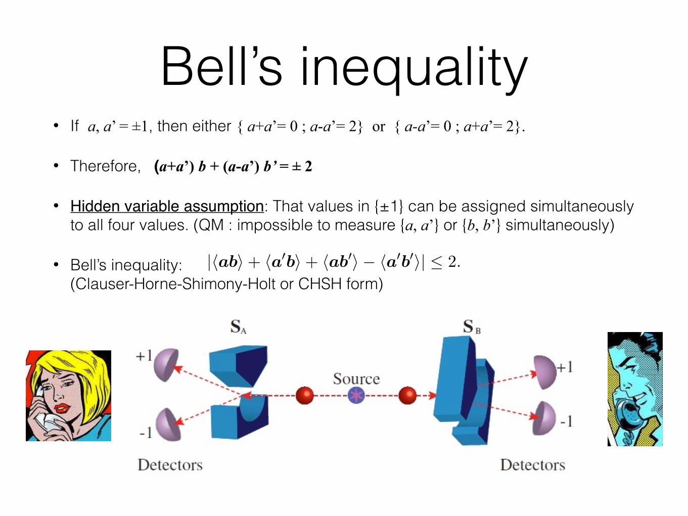
Bell’s inequality• If a, a’ = ±1, then either { a+a’= 0 ; a-a’= 2} or { a-a’= 0 ; a+a’= 2}.
• Therefore, (a+a’) b + (a-a’) b’ = ± 2
• Hidden variable assumption: That values in {±1} can be assigned simultaneously to all four values. (QM : impossible to measure {a, a’} or {b, b’} simultaneously)
• Bell’s inequality: (Clauser-Horne-Shimony-Holt or CHSH form)
4.3 More Bell inequalities 17
ing a more complete, yet still local, description of Nature. If we acceptlocality as an inviolable principle, then we are forced to accept random-ness as an unavoidable and intrinsic feature of quantum measurement,rather than a consequence of incomplete knowledge.
To some, the peculiar correlations unmasked by Bell’s inequality callout for a deeper explanation than quantum mechanics seems to provide.They see the EPR phenomenon as a harbinger of new physics awaitingdiscovery. But they may be wrong. We have been waiting over 65 yearssince EPR, and so far no new physics.
The human mind seems to be poorly equipped to grasp the correlationsexhibited by entangled quantum states, and so we speak of the weirdnessof quantum theory. But whatever your attitude, experiment forces youto accept the existence of the weird correlations among the measurementoutcomes. There is no big mystery about how the correlations were estab-lished — we saw that it was necessary for Alice and Bob to get togetherat some point to create entanglement among their qubits. The novelty isthat, even when A and B are distantly separated, we cannot accuratelyregard A and B as two separate qubits, and use classical information tocharacterize how they are correlated. They are more than just correlated,they are a single inseparable entity. They are entangled.
4.3 More Bell inequalities
4.3.1 CHSH inequality
Experimental tests of Einstein locality typically are based on anotherform of the Bell inequality, which applies to a situation in which Alice canmeasure either one of two observables a and a′, while Bob can measureeither b or b′. Suppose that the observables a, a′, b, b′ take values in{±1}, and are functions of hidden random variables.
If a, a′ = ±1, it follows that either a+a′ = 0, in which case a−a′ = ±2,or else a − a′ = 0, in which case a + a′ = ±2; therefore
C ≡ (a + a′)b + (a− a′)b′ = ±2 . (4.31)
(Here is where the local hidden-variable assumption sneaks in — we haveimagined that values in {±1} can be assigned simultaneously to all fourobservables, even though it is impossible to measure both of a and a′, orboth of b and b′.) Evidently
|⟨C⟩| ≤ ⟨|C|⟩ = 2, (4.32)
so that
|⟨ab⟩ + ⟨a′b⟩ + ⟨ab′⟩ − ⟨a′b′⟩| ≤ 2. (4.33)
Quantum Mechanical prediction• QM state of entangled particles:
• If Alice measures in direction n and gets spin-up, then state becomes:
• Say Bob chose to measure in direction n’.
• Based on what we know, we can calculate the probabilities.
QM prediction for
a’ b probability+1 -1 50%-1 +1 50%+1 +1 0%-1 -1 0%
This result is called the CHSH inequality (for Clauser-Horne-Shimony-Holt). It holds for any random variables a, a′, b, b′ taking values in ±1that are governed by a joint probability distribution.
To see that quantum mechanics violates the CHSH inequality, let a, a′
denote the Hermitian operators
a = σ(A) · a , a′ = σ(A) · a′ , (4.34)
acting on a qubit in Alice’s possession, where a, a′ are unit 3-vectors.Similarly, let b, b′ denote
b = σ(B) · b , b′ = σ(B) · b′ , (4.35)
acting on Bob’s qubit. Each observable has eigenvalues ±1 so that anoutcome of a measurement of the observable takes values in ±1.
Recall that if Alice and Bob share the maximally-entangled state |ψ−⟩,then
⟨ψ−|!
σ(A) · a"!
σ(B) · b"
|ψ−⟩ = −a · b = − cos θ ,(4.36)
where θ is the angle between a and b. Consider the case where a′, b, a, b′
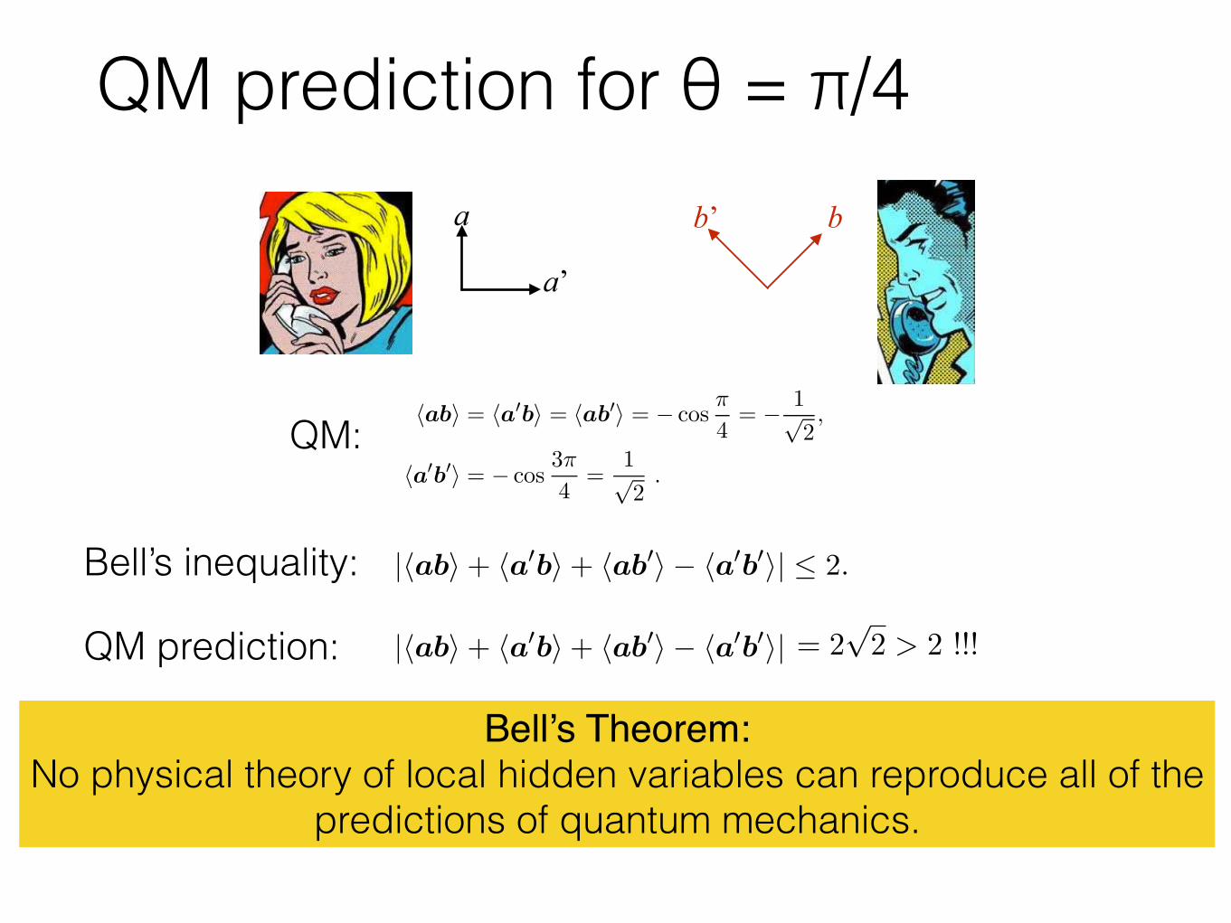
are coplanar and separated by successive 45◦ angles. so that the quantum-mechanical predictions are
⟨ab⟩ = ⟨a′b⟩ = ⟨ab′⟩ = − cosπ
4= − 1√
2,
⟨a′b′⟩ = − cos3π
4=
1√2
. (4.37)
The CHSH inequality then becomes
4 ·1√2
= 2√
2 ≤ 2 , (4.38)
which is clearly violated by the quantum-mechanical prediction.
4.3.2 Maximal violation
In fact the case just considered provides the largest possible quantum-mechanical violation of the CHSH inequality, as we can see by the fol-lowing argument. Suppose that a, a′, b, b′ are Hermitian operators witheigenvalues ±1, so that
a2 = a′2 = b2 = b′2 = I , (4.39)
4.3 More Bell inequalities 17
ing a more complete, yet still local, description of Nature. If we acceptlocality as an inviolable principle, then we are forced to accept random-ness as an unavoidable and intrinsic feature of quantum measurement,rather than a consequence of incomplete knowledge.
To some, the peculiar correlations unmasked by Bell’s inequality callout for a deeper explanation than quantum mechanics seems to provide.They see the EPR phenomenon as a harbinger of new physics awaitingdiscovery. But they may be wrong. We have been waiting over 65 yearssince EPR, and so far no new physics.
The human mind seems to be poorly equipped to grasp the correlationsexhibited by entangled quantum states, and so we speak of the weirdnessof quantum theory. But whatever your attitude, experiment forces youto accept the existence of the weird correlations among the measurementoutcomes. There is no big mystery about how the correlations were estab-lished — we saw that it was necessary for Alice and Bob to get togetherat some point to create entanglement among their qubits. The novelty isthat, even when A and B are distantly separated, we cannot accuratelyregard A and B as two separate qubits, and use classical information tocharacterize how they are correlated. They are more than just correlated,they are a single inseparable entity. They are entangled.
4.3 More Bell inequalities
4.3.1 CHSH inequality
Experimental tests of Einstein locality typically are based on anotherform of the Bell inequality, which applies to a situation in which Alice canmeasure either one of two observables a and a′, while Bob can measureeither b or b′. Suppose that the observables a, a′, b, b′ take values in{±1}, and are functions of hidden random variables.
If a, a′ = ±1, it follows that either a+a′ = 0, in which case a−a′ = ±2,or else a − a′ = 0, in which case a + a′ = ±2; therefore
C ≡ (a + a′)b + (a− a′)b′ = ±2 . (4.31)
(Here is where the local hidden-variable assumption sneaks in — we haveimagined that values in {±1} can be assigned simultaneously to all fourobservables, even though it is impossible to measure both of a and a′, orboth of b and b′.) Evidently
Bell’s Theorem: No physical theory of local hidden variables can reproduce all of the
predictions of quantum mechanics.
4.3 More Bell inequalities 17
ing a more complete, yet still local, description of Nature. If we acceptlocality as an inviolable principle, then we are forced to accept random-ness as an unavoidable and intrinsic feature of quantum measurement,rather than a consequence of incomplete knowledge.
To some, the peculiar correlations unmasked by Bell’s inequality callout for a deeper explanation than quantum mechanics seems to provide.They see the EPR phenomenon as a harbinger of new physics awaitingdiscovery. But they may be wrong. We have been waiting over 65 yearssince EPR, and so far no new physics.
The human mind seems to be poorly equipped to grasp the correlationsexhibited by entangled quantum states, and so we speak of the weirdnessof quantum theory. But whatever your attitude, experiment forces youto accept the existence of the weird correlations among the measurementoutcomes. There is no big mystery about how the correlations were estab-lished — we saw that it was necessary for Alice and Bob to get togetherat some point to create entanglement among their qubits. The novelty isthat, even when A and B are distantly separated, we cannot accuratelyregard A and B as two separate qubits, and use classical information tocharacterize how they are correlated. They are more than just correlated,they are a single inseparable entity. They are entangled.
4.3 More Bell inequalities
4.3.1 CHSH inequality
Experimental tests of Einstein locality typically are based on anotherform of the Bell inequality, which applies to a situation in which Alice canmeasure either one of two observables a and a′, while Bob can measureeither b or b′. Suppose that the observables a, a′, b, b′ take values in{±1}, and are functions of hidden random variables.
If a, a′ = ±1, it follows that either a+a′ = 0, in which case a−a′ = ±2,or else a − a′ = 0, in which case a + a′ = ±2; therefore
C ≡ (a + a′)b + (a− a′)b′ = ±2 . (4.31)
(Here is where the local hidden-variable assumption sneaks in — we haveimagined that values in {±1} can be assigned simultaneously to all fourobservables, even though it is impossible to measure both of a and a′, orboth of b and b′.) Evidently
|⟨C⟩| ≤ ⟨|C|⟩ = 2, (4.32)
so that
|⟨ab⟩ + ⟨a′b⟩ + ⟨ab′⟩ − ⟨a′b′⟩| ≤ 2. (4.33)= 2�
2 > 2 !!!
QM:
QM prediction for θ = π/4a
a’
bb’θ = π/4
18 4 Quantum Entanglement
This result is called the CHSH inequality (for Clauser-Horne-Shimony-Holt). It holds for any random variables a, a′, b, b′ taking values in ±1that are governed by a joint probability distribution.
To see that quantum mechanics violates the CHSH inequality, let a, a′
denote the Hermitian operators
a = σ(A) · a , a′ = σ(A) · a′ , (4.34)
acting on a qubit in Alice’s possession, where a, a′ are unit 3-vectors.Similarly, let b, b′ denote
b = σ(B) · b , b′ = σ(B) · b′ , (4.35)
acting on Bob’s qubit. Each observable has eigenvalues ±1 so that anoutcome of a measurement of the observable takes values in ±1.
Recall that if Alice and Bob share the maximally-entangled state |ψ−⟩,then
⟨ψ−|!
σ(A) · a"!
σ(B) · b"
|ψ−⟩ = −a · b = − cos θ ,(4.36)
where θ is the angle between a and b. Consider the case where a′, b, a, b′
are coplanar and separated by successive 45◦ angles. so that the quantum-mechanical predictions are
⟨ab⟩ = ⟨a′b⟩ = ⟨ab′⟩ = − cosπ
4= − 1√
2,
⟨a′b′⟩ = − cos3π
4=
1√2
. (4.37)
The CHSH inequality then becomes
4 ·1√2
= 2√
2 ≤ 2 , (4.38)
which is clearly violated by the quantum-mechanical prediction.
4.3.2 Maximal violation
In fact the case just considered provides the largest possible quantum-mechanical violation of the CHSH inequality, as we can see by the fol-lowing argument. Suppose that a, a′, b, b′ are Hermitian operators witheigenvalues ±1, so that
a2 = a′2 = b2 = b′2 = I , (4.39)
4.3 More Bell inequalities 17
ing a more complete, yet still local, description of Nature. If we acceptlocality as an inviolable principle, then we are forced to accept random-ness as an unavoidable and intrinsic feature of quantum measurement,rather than a consequence of incomplete knowledge.
To some, the peculiar correlations unmasked by Bell’s inequality callout for a deeper explanation than quantum mechanics seems to provide.They see the EPR phenomenon as a harbinger of new physics awaitingdiscovery. But they may be wrong. We have been waiting over 65 yearssince EPR, and so far no new physics.
The human mind seems to be poorly equipped to grasp the correlationsexhibited by entangled quantum states, and so we speak of the weirdnessof quantum theory. But whatever your attitude, experiment forces youto accept the existence of the weird correlations among the measurementoutcomes. There is no big mystery about how the correlations were estab-lished — we saw that it was necessary for Alice and Bob to get togetherat some point to create entanglement among their qubits. The novelty isthat, even when A and B are distantly separated, we cannot accuratelyregard A and B as two separate qubits, and use classical information tocharacterize how they are correlated. They are more than just correlated,they are a single inseparable entity. They are entangled.
4.3 More Bell inequalities
4.3.1 CHSH inequality
Experimental tests of Einstein locality typically are based on anotherform of the Bell inequality, which applies to a situation in which Alice canmeasure either one of two observables a and a′, while Bob can measureeither b or b′. Suppose that the observables a, a′, b, b′ take values in{±1}, and are functions of hidden random variables.
If a, a′ = ±1, it follows that either a+a′ = 0, in which case a−a′ = ±2,or else a − a′ = 0, in which case a + a′ = ±2; therefore
C ≡ (a + a′)b + (a− a′)b′ = ±2 . (4.31)
(Here is where the local hidden-variable assumption sneaks in — we haveimagined that values in {±1} can be assigned simultaneously to all fourobservables, even though it is impossible to measure both of a and a′, orboth of b and b′.) Evidently
Bell’s Theorem: No physical theory of local hidden variables can reproduce all of the
predictions of quantum mechanics.
4.3 More Bell inequalities 17
ing a more complete, yet still local, description of Nature. If we acceptlocality as an inviolable principle, then we are forced to accept random-ness as an unavoidable and intrinsic feature of quantum measurement,rather than a consequence of incomplete knowledge.
To some, the peculiar correlations unmasked by Bell’s inequality callout for a deeper explanation than quantum mechanics seems to provide.They see the EPR phenomenon as a harbinger of new physics awaitingdiscovery. But they may be wrong. We have been waiting over 65 yearssince EPR, and so far no new physics.
The human mind seems to be poorly equipped to grasp the correlationsexhibited by entangled quantum states, and so we speak of the weirdnessof quantum theory. But whatever your attitude, experiment forces youto accept the existence of the weird correlations among the measurementoutcomes. There is no big mystery about how the correlations were estab-lished — we saw that it was necessary for Alice and Bob to get togetherat some point to create entanglement among their qubits. The novelty isthat, even when A and B are distantly separated, we cannot accuratelyregard A and B as two separate qubits, and use classical information tocharacterize how they are correlated. They are more than just correlated,they are a single inseparable entity. They are entangled.
4.3 More Bell inequalities
4.3.1 CHSH inequality
Experimental tests of Einstein locality typically are based on anotherform of the Bell inequality, which applies to a situation in which Alice canmeasure either one of two observables a and a′, while Bob can measureeither b or b′. Suppose that the observables a, a′, b, b′ take values in{±1}, and are functions of hidden random variables.
If a, a′ = ±1, it follows that either a+a′ = 0, in which case a−a′ = ±2,or else a − a′ = 0, in which case a + a′ = ±2; therefore
C ≡ (a + a′)b + (a− a′)b′ = ±2 . (4.31)
(Here is where the local hidden-variable assumption sneaks in — we haveimagined that values in {±1} can be assigned simultaneously to all fourobservables, even though it is impossible to measure both of a and a′, orboth of b and b′.) Evidently
|⟨C⟩| ≤ ⟨|C|⟩ = 2, (4.32)
so that
|⟨ab⟩ + ⟨a′b⟩ + ⟨ab′⟩ − ⟨a′b′⟩| ≤ 2. (4.33)= 2�
2 > 2 !!!
QM:
QM prediction for θ = π/4 (some math)
a
a’
bb’
18 4 Quantum Entanglement
This result is called the CHSH inequality (for Clauser-Horne-Shimony-Holt). It holds for any random variables a, a′, b, b′ taking values in ±1that are governed by a joint probability distribution.
To see that quantum mechanics violates the CHSH inequality, let a, a′
denote the Hermitian operators
a = σ(A) · a , a′ = σ(A) · a′ , (4.34)
acting on a qubit in Alice’s possession, where a, a′ are unit 3-vectors.Similarly, let b, b′ denote
b = σ(B) · b , b′ = σ(B) · b′ , (4.35)
acting on Bob’s qubit. Each observable has eigenvalues ±1 so that anoutcome of a measurement of the observable takes values in ±1.
Recall that if Alice and Bob share the maximally-entangled state |ψ−⟩,then
⟨ψ−|!
σ(A) · a"!
σ(B) · b"
|ψ−⟩ = −a · b = − cos θ ,(4.36)
where θ is the angle between a and b. Consider the case where a′, b, a, b′
are coplanar and separated by successive 45◦ angles. so that the quantum-mechanical predictions are
⟨ab⟩ = ⟨a′b⟩ = ⟨ab′⟩ = − cosπ
4= − 1√
2,
⟨a′b′⟩ = − cos3π
4=
1√2
. (4.37)
The CHSH inequality then becomes
4 ·1√2
= 2√
2 ≤ 2 , (4.38)
which is clearly violated by the quantum-mechanical prediction.
4.3.2 Maximal violation
In fact the case just considered provides the largest possible quantum-mechanical violation of the CHSH inequality, as we can see by the fol-lowing argument. Suppose that a, a′, b, b′ are Hermitian operators witheigenvalues ±1, so that
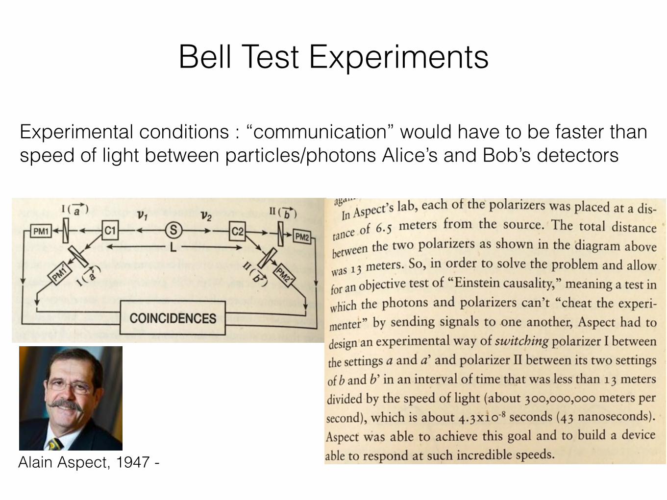
Experimental conditions : “communication” would have to be faster than speed of light between particles/photons Alice’s and Bob’s detectors
Alain Aspect, 1947 -
Bell Test Experiments
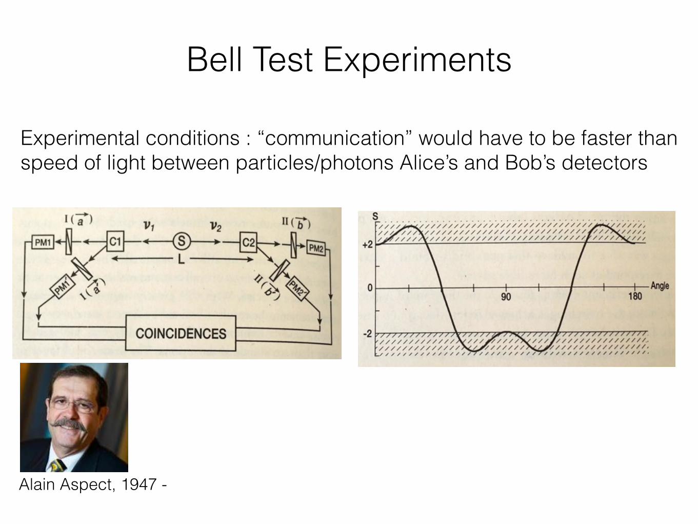
Experimental conditions : “communication” would have to be faster than speed of light between particles/photons Alice’s and Bob’s detectors
Alain Aspect, 1947 -
Bell Test Experiments
Experimental conditions : “communication” would have to be faster than speed of light between particles/photons Alice’s and Bob’s detectors
Alain Aspect, 1947 -
One expt: 2.25 ± 0.03 : violation of Bell’s inequality!
More Bell Test Experiments
Experimental conditions rule out locality, i.e. “communication” at speed of light between photons at Alice’s and Bob’s detectors
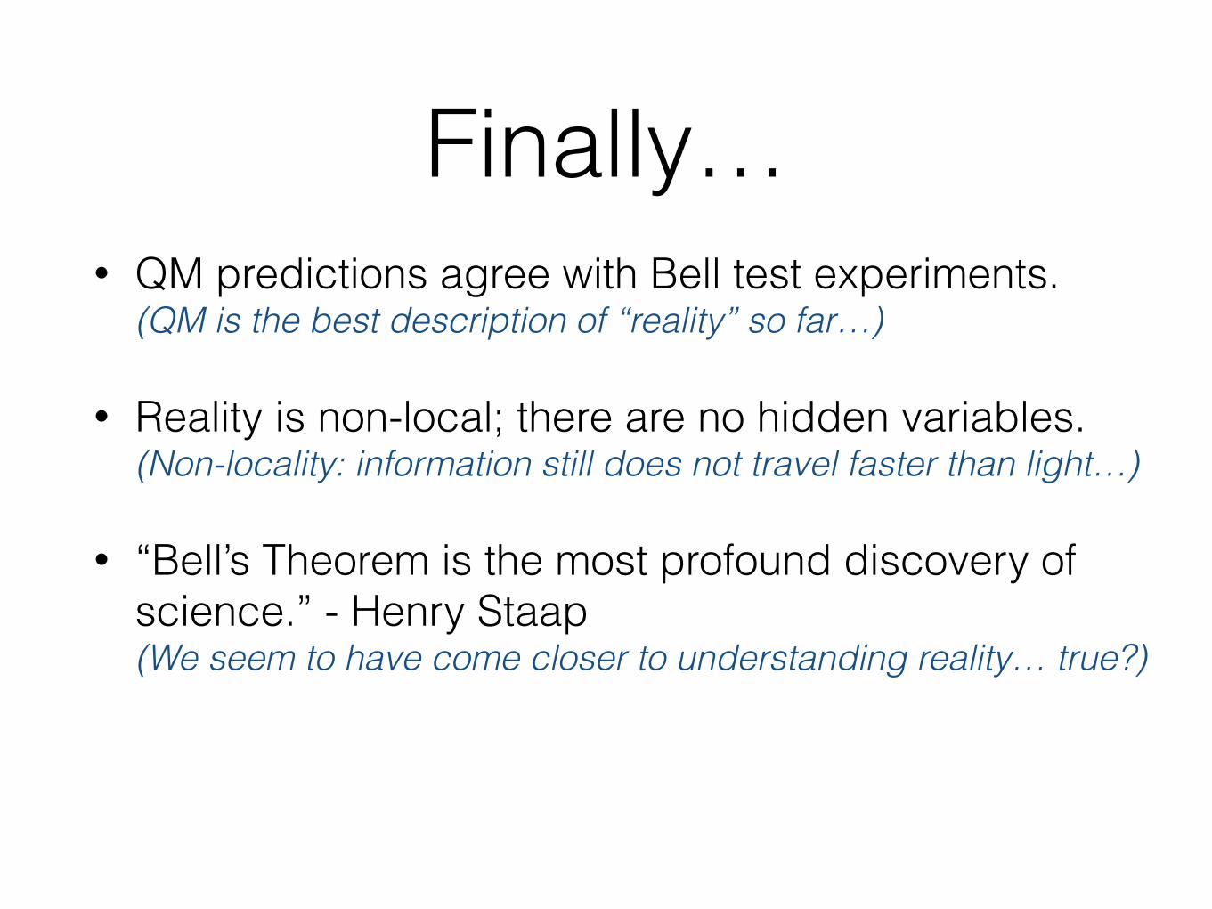
Finally…
Finally…• QM predictions agree with Bell test experiments.
(QM is the best description of “reality” so far…)
Finally…• QM predictions agree with Bell test experiments.
(QM is the best description of “reality” so far…)
• Reality is non-local; there are no hidden variables. (Non-locality: information still does not travel faster than light…)
Finally…• QM predictions agree with Bell test experiments.
(QM is the best description of “reality” so far…)
• Reality is non-local; there are no hidden variables. (Non-locality: information still does not travel faster than light…)
• “Bell’s Theorem is the most profound discovery of science.” - Henry Staap(We seem to have come closer to understanding reality… true?)
• Is the moon there when nobody looks at it? — Einstein to Mermin
Open questions• Loopholes in experiment- locality loophole (just now) - fair sampling loophole (instruments detect subsample; particles not always detected in both wings of apparatus) - free will loophole (results are predetermined by “higher power”; the “universe” already “knows” the outcome)
• Quantum-Classical Boundary?- No macroscopic superposition (i.e. no dead+alive cat!) - Decoherence
• Other interpretations of QM- Consistent histories- Many-worlds (Everett)
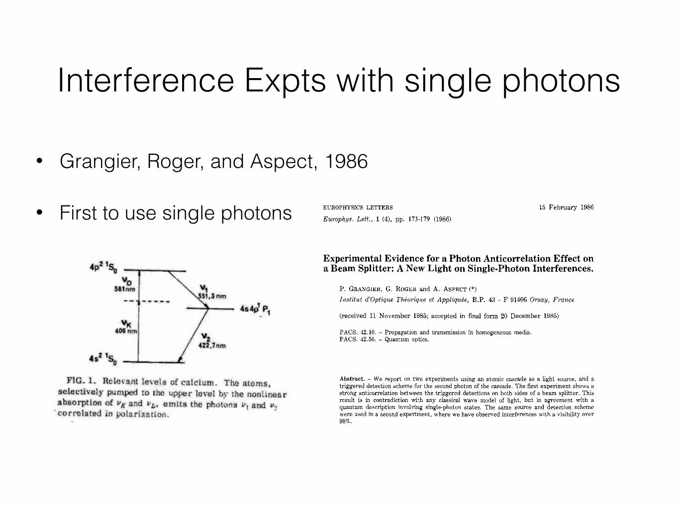
Interference Expts with single photons
• Grangier, Roger, and Aspect, 1986
• First to use single photons EUROPHYSICS LETTERS
Europhys. Lett., 1 (4), pp. 173-179 (1986) 15 February 1986
Experimental Evidence for a Photon Anticorrelation Effect on a Beam Splitter: A New Light on Single-Photon Interferences.
P. GRANGIER, G. ROGER and A. ASPECT (*) Ins t i tu t d’0ptique Thhorique et Appliquhe, B.P. 43 - F 91406 Orsay , France
(received 11 November 1985; accepted in final form 20 December 1985)
PACS. 42.10. - Propagation and transmission in homogeneous media. PACS. 42.50. - Quantum optics.
Abstract. - We report on two experiments using an atomic cascade as a light source, and a triggered detection scheme for the second photon of the cascade. The first experiment shows a strong anticorrelation between the triggered detections on both sides of a beam splitter. This result is in contradiction with any classical wave model of light, but in agreement with a quantum description involving single-photon states. The same source and detection scheme were used in a second experiment, where we have observed interferences with a visibility over 98%.
During the past fifteen years, nonclassical effects in the statistical properties of light have been extensively studied from a theoretical point of view [l], and some have been experimentally demonstrated [2-71. All are related to second-order coherence properties, via measurements of intensity correlation functions or of statistical moments. However, there has still been no test of the conceptually very simple situation dealing with single- photon states of the light impinging on a beam splitter. In this case, quantum mechanics predicts a perfect anticorrelation for photodetections on both sides of the beam splitter (a single-photon can only be detected once!), while any description involving classical fields would predict some amount of coincidences. In the first part of this letter, we report on an experiment close to this ideal situation, since we have found a coincidence rate, on both sides of a beam splitter, five times smaller than the classical lower limit.
When it comes to single-photon states of light, it is tempting to revisit the famous historical .single-photon interference experiments. [8]. One then finds that, in spite of their
(*) Also with College de France, Laboratoire de Spectroscopie Hertzienne de l’ENS, 24 rue Lhomond, 75005 Paris 5eme.