115
Quantum Thermodynamics An introduction to the thermodynamics of quantum information Sebastian Deffner and Steve Campbell July 4, 2019 arXiv:1907.01596v1 [quant-ph] 2 Jul 2019
Quantum ThermodynamicsAn introduction to the thermodynamics of quantum information
Sebastian Deffner and Steve Campbell
July 4, 2019
arX
iv:1
907.
0159
6v1
[qu
ant-
ph]
2 J
ul 2
019
Abstract
This book provides an introduction to the emerging field of quantum thermodynamics, with particu-lar focus on its relation to quantum information and its implications for quantum computers and nextgeneration quantum technologies. The text, aimed at graduate level physics students with a workingknowledge of quantum mechanics and statistical physics, provides a brief overview of the develop-ment of classical thermodynamics and its quantum formulation in Chapter 1. Chapter 2 then explorestypical thermodynamic settings, such as cycles and work extraction protocols, when the working ma-terial is genuinely quantum. Finally, Chapter 3 explores the thermodynamics of quantum informationprocessing and introduces the reader to some more state-of-the-art topics in this exciting and rapidlydeveloping research field.
II

III
Quidquid praecipies, esto brevis.(Horaz, Ars poetica 335)
About the Authors
Sebastian Deffner
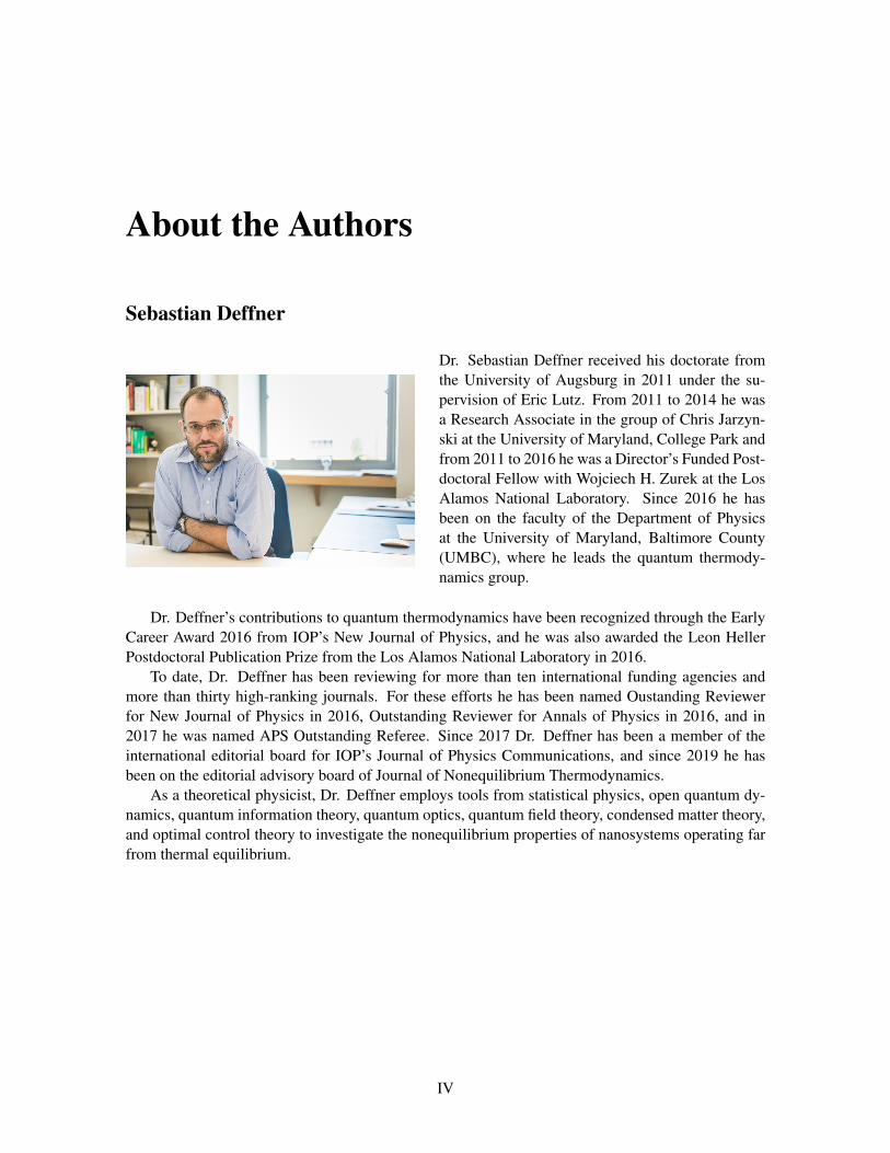
Dr. Sebastian Deffner received his doctorate fromthe University of Augsburg in 2011 under the su-pervision of Eric Lutz. From 2011 to 2014 he wasa Research Associate in the group of Chris Jarzyn-ski at the University of Maryland, College Park andfrom 2011 to 2016 he was a Director’s Funded Post-doctoral Fellow with Wojciech H. Zurek at the LosAlamos National Laboratory. Since 2016 he hasbeen on the faculty of the Department of Physicsat the University of Maryland, Baltimore County(UMBC), where he leads the quantum thermody-namics group.
Dr. Deffner’s contributions to quantum thermodynamics have been recognized through the EarlyCareer Award 2016 from IOP’s New Journal of Physics, and he was also awarded the Leon HellerPostdoctoral Publication Prize from the Los Alamos National Laboratory in 2016.
To date, Dr. Deffner has been reviewing for more than ten international funding agencies andmore than thirty high-ranking journals. For these efforts he has been named Oustanding Reviewerfor New Journal of Physics in 2016, Outstanding Reviewer for Annals of Physics in 2016, and in2017 he was named APS Outstanding Referee. Since 2017 Dr. Deffner has been a member of theinternational editorial board for IOP’s Journal of Physics Communications, and since 2019 he hasbeen on the editorial advisory board of Journal of Nonequilibrium Thermodynamics.
As a theoretical physicist, Dr. Deffner employs tools from statistical physics, open quantum dy-namics, quantum information theory, quantum optics, quantum field theory, condensed matter theory,and optimal control theory to investigate the nonequilibrium properties of nanosystems operating farfrom thermal equilibrium.
IV

V
Steve Campbell
After a PhD in Queens University Belfast in 2011 underthe supervision of Mauro Paternostro, Dr. Steve Campbellmoved to University College Cork to work with ThomasBusch in 2012. He spent 2013 at the Okinawa Instituteof Science and Technology Graduate University in Japan.Returning to Belfast, he spent 2014 through to 2016 at hisalma mater Queens University. In 2017 he was awarded afellowship from the INFN Sezione di Milano and workedwith Bassano Vacchini. From February 2019 he has beenappointed as Senior Research Fellow at Trinity CollegeDublin through the award of a Science Foundation IrelandStarting Investigators Research Grant.
Dr. Campbell is interested in exploring the role which fundamental bounds, such as the quantumspeed limit, play in characterizing and designing thermodynamically efficient control protocols forcomplex quantum systems. He works on a variety of topics including open quantum systems, criticalspin systems and phase transitions, metrology, and coherent control.
Contents
Abstract II
About the Authors IV
Prologue 1
1 The principles of modern thermodynamics 51.1 A phenomenological theory of heat and work . . . . . . . . . . . . . . . . . . . . . 5
1.1.1 The five laws of thermodynamics . . . . . . . . . . . . . . . . . . . . . . . 51.1.2 Finite-time thermodynamics and endoreversibility . . . . . . . . . . . . . . 10
1.2 The advent of Stochastic Thermodynamics . . . . . . . . . . . . . . . . . . . . . . 121.2.1 Microscopic dynamics . . . . . . . . . . . . . . . . . . . . . . . . . . . . . 131.2.2 Stochastic energetics . . . . . . . . . . . . . . . . . . . . . . . . . . . . . . 151.2.3 Jarzynski equality and Crooks theorem . . . . . . . . . . . . . . . . . . . . 15
1.3 Foundations of statistical physics from quantum entanglement . . . . . . . . . . . . 191.3.1 Entanglement assisted invariance . . . . . . . . . . . . . . . . . . . . . . . 191.3.2 Microcanonical state from envariance . . . . . . . . . . . . . . . . . . . . . 201.3.3 Canonical state from quantum envariance . . . . . . . . . . . . . . . . . . . 21
1.4 Work, heat, and entropy production . . . . . . . . . . . . . . . . . . . . . . . . . . 231.4.1 Quantum work and quantum heat . . . . . . . . . . . . . . . . . . . . . . . 241.4.2 Quantum entropy production . . . . . . . . . . . . . . . . . . . . . . . . . . 261.4.3 Two-time energy measurement approach . . . . . . . . . . . . . . . . . . . 271.4.4 Quantum fluctuation theorem for arbitrary observables . . . . . . . . . . . . 311.4.5 Quantum entropy production in phase space . . . . . . . . . . . . . . . . . 32
1.5 Checklist for “The principles of modern thermodynamics” . . . . . . . . . . . . . . 351.6 Problems . . . . . . . . . . . . . . . . . . . . . . . . . . . . . . . . . . . . . . . . 35References . . . . . . . . . . . . . . . . . . . . . . . . . . . . . . . . . . . . . . . . . . . 36
2 Thermodynamics of Quantum Systems 412.1 Quantum thermometry . . . . . . . . . . . . . . . . . . . . . . . . . . . . . . . . . 41
2.1.1 Thermometry for Harmonic Spectra . . . . . . . . . . . . . . . . . . . . . . 432.1.2 Optimal Thermometers . . . . . . . . . . . . . . . . . . . . . . . . . . . . . 44
2.2 Quantum heat engines – engines with atomic working fluids . . . . . . . . . . . . . 452.2.1 The Otto Cycle: Classical to quantum formulation . . . . . . . . . . . . . . 452.2.2 A two-level Otto cycle . . . . . . . . . . . . . . . . . . . . . . . . . . . . . 472.2.3 Endoreversible Otto cycle . . . . . . . . . . . . . . . . . . . . . . . . . . . 50
2.3 Work extraction from quantum systems . . . . . . . . . . . . . . . . . . . . . . . . 542.3.1 Work extraction from arrays of quantum batteries . . . . . . . . . . . . . . . 56
VI
CONTENTS VII
2.3.2 Powerful charging of quantum batteries . . . . . . . . . . . . . . . . . . . . 592.4 Quantum decoherence and the tale of quantum Darwinism . . . . . . . . . . . . . . 60
2.4.1 Work, heat, and entropy production for dynamical semigroups . . . . . . . . 602.4.2 Entropy production as correlation . . . . . . . . . . . . . . . . . . . . . . . 622.4.3 Quantum Darwinism: Emergence of classical objectivity . . . . . . . . . . . 63
2.5 Checklist for “Thermodynamics of Quantum Systems” . . . . . . . . . . . . . . . . 682.6 Problems . . . . . . . . . . . . . . . . . . . . . . . . . . . . . . . . . . . . . . . . 68References . . . . . . . . . . . . . . . . . . . . . . . . . . . . . . . . . . . . . . . . . . . 69
3 Thermodynamics of Quantum Information 743.1 Quantum thermodynamics of information . . . . . . . . . . . . . . . . . . . . . . . 74
3.1.1 Thermodynamics of classical information processing . . . . . . . . . . . . . 743.1.2 A quantum sharpening of Landauer’s bound . . . . . . . . . . . . . . . . . . 783.1.3 New Landauer bounds for non-equilibrium quantum systems . . . . . . . . . 80
3.2 Performance diagnostics of quantum annealers . . . . . . . . . . . . . . . . . . . . 813.2.1 Fluctuation theorem for quantum annealers . . . . . . . . . . . . . . . . . . 823.2.2 Experimental test on the D-Wave machine . . . . . . . . . . . . . . . . . . . 83
3.3 Kibble-Zurek Scaling of Irreversible Entropy . . . . . . . . . . . . . . . . . . . . . 853.3.1 Fundamentals of the Kibble-Zurek mechanism . . . . . . . . . . . . . . . . 863.3.2 Example: the Landau-Zener model . . . . . . . . . . . . . . . . . . . . . . 873.3.3 Kibble-Zurek mechanism and entropy production . . . . . . . . . . . . . . . 88
3.4 Error correction in adiabatic quantum computers . . . . . . . . . . . . . . . . . . . 903.4.1 Quantum error correction in quantum annealers . . . . . . . . . . . . . . . . 923.4.2 Adiabatic quantum computing – A case for shortcuts to adiabaticity . . . . . 933.4.3 Counterdiabatic Hamiltonian for scale-invariant driving . . . . . . . . . . . . 94
3.5 Checklist for “Thermodynamics of Quantum Information” . . . . . . . . . . . . . . 993.6 Problems . . . . . . . . . . . . . . . . . . . . . . . . . . . . . . . . . . . . . . . . 99References . . . . . . . . . . . . . . . . . . . . . . . . . . . . . . . . . . . . . . . . . . . 100
Epilogue 106
Acknowledgments 107

VIII CONTENTS
Prologue
What is physics? According to standard definitions in encyclopedias physics is a science that dealswith matter and energy and their interactions1. However, as physicists what is that we actually do?At the most basic level, we formulate predictions for how inanimate objects behave in their naturalsurroundings. These predictions are based on our expectation that we extrapolate from observationsof the typical behavior. If typical behavior is universally exhibited by many systems of the same“family”, then this typical behavior is phrased as a law.
Take for instance the infamous example of an apple falling from a tree. The same behavior isobserved for any kind of fruit and any kind of tree – the fruit “always” falls from the tree to theground. Well, actually the same behavior is observed for any object that is let loose above the ground,namely everything will eventually fall towards the ground. It is this observation of universal fallingthat is encoded in the law of gravity.
Most theories in physics then seek to understand the nitty-gritty details, for which finer and moreaccurate observations are essential. Generally, we end up with more and more fine-grained descrip-tions of nature that are packed into more and more sophisticated laws. For instance, from classicalmechanics over quantum mechanics to quantum field theory we obtain an ever more detailed predic-tion for how smaller and smaller systems behave.
Realizing this typical mindset of physical theories, it does not come as a big surprise that manystudents have such a hard time wrapping their minds around thermodynamics:
Thermodynamics is a phenomenological theory to describe the average behavior of heatand work.
As a phenomenological theory, thermodynamics does not seek to formulate detailed predictions forthe microscopic behavior of some physical systems, but rather it aims to provide the most universalframework to describe the typical behavior of all physical systems.
“Reflections on the Motive Power of Fire”. The origins of thermodynamics trace back to thebeginnings of the industrial revolution [6]. For the first time, mankind started developing artificialdevices that contained so many moving parts that it became practically impossible to describe theirbehavior in full detail. Nevertheless, already the first devices, steam engines, proved to be remarkablyuseful and dramatically increased the effectiveness of productive efforts.
The founding father of thermodynamics is undoubtedly Sadi Carnot. After Napoleon had beenexiled, France started importing advanced steam engines from Britain, which made Carnot realizehow far France had fallen behind its adversary from across the channel. Quite remarkably, a smallnumber of British engineers, who totally lacked any formal scientific education, had started to collectreliable data about the efficiency of many types of steam engines. However, it was not at all clearwhether there was an optimal design and what the highest efficiency would be.
1This and similar definitions can be found, for instance, in Merriam-Webster.
1
2
Nicolas Leonard Sadi Carnot:Everyone knows that heat can produce motion [2].
Carnot had been trained in the latest developments in physics and chemistry, and it was he whorecognized that steam engines need to be understood in terms of their energy balance. Thus, optimiz-ing steam engines was not only a matter of improving the expansion and compression of steam, butactually needed an understanding of the relationship between work and heat [2].
Sadly, Carnot’s work [2] was largely ignored by the scientific community until the railroad en-gineer Emile Clapeyron quoted and generalized Carnot’s results. Eventually 30 years later, it wasRudolph Clausius, who put Carnot’s insight into a solid mathematical framework [3], which is thesame mathematical theory that we still use today – thermodynamics.
Thus, thermodynamics is not only unique among the theories in physics with respect to its mind-set, but also with respect to its beginnings. No other theory is so intimately connected with someonenever holding an academic position – Sadi Carnot. Formulating the original ideas was thus largelymotivated by practical questions and not purely by scientific curiosity. This might explain why morethan any other theory thermodynamics is a framework to describe the typical and universal behaviorof any physical system.
Quantum computing – Feynman’s dream come true. A remarkable quote from Carnot’s work [2]is the following:
The study of these engines is of the greatest interest, their importance is enormous, theiruse is continually increasing, and they seem destined to produce a great revolution in thecivilized world.
If we replaced the word “engines” with “quantum computers”, Carnot’s sentence would fit nicely intothe announcements of the various “quantum initiatives” around the globe [7].
Ever since Feyman’s proposal in the early 1980s [4] quantum computing as been a promise thatcould initiate a technological revolution. Over the last couple of years big corporations, such asMicrosoft, IBM and Google, as well as smaller start-ups, such as D-Wave or Rigetti, have started topresent more and more intricate technologies that promise to eventually lead to the development of apractically useful quantum computer.
Rather curiously, we are in a very similar situation that Carnot found in the beginning of the 19thcentury. Novel technologies are being developed by crafty engineers that are much too complicatedto be described in full microscopic detail. Nevertheless, the question that we are really after is howto operate these technologies optimally in the sense that the least amount of resources, such as workand information, are wasted into the environment.
As physicists we know exactly which theory will prevail in the attempt to describe what is goingon, since it is the only theory that is universal enough to be useful when faced with new challenges
3
Richard P. Feynman:Nature isn’t classical, dammit, and if you want to makea simulation of nature, you’d better make it quantummechanical, and by golly it’s a wonderful problem, be-cause it doesn’t look so easy [4].
– thermodynamics. However, this time the natural variables can no longer be volume, temperature,and pressure, which are characteristic for steam engines. Rather, in Quantum Thermodynamics thefirst task has to be to identify the new canonical variables, and then write the dictionary for how totranslate between the universal thermodynamic framework and practically useful statements for theoptimization of quantum technologies.
Purpose and target audience of this book. The purpose of this book is to provide a concise in-troduction to the conceptual building blocks of Quantum Thermodynamics and their application inthe description of quantum systems that process information. Large parts of this book arose from ourlecture notes that we had put together for graduate classes in statistical physics or for workshops andsummer schools dedicated to Quantum Thermodynamics. When teaching the various topics of Quan-tum Thermodynamics we always felt a bit unsatisfied as no single book contained a comprehensiveoverview of all the topics we deemed essential. Earlier monographs have become a bit outdated, suchas Quantum Thermodynamics by our colleagues Gemmer, Michel, and Mahler [5], or are simply notwritten as a textbook suited for teaching, such as Thermodynamics in the Quantum Regime which wasedited by Binder et al. [1].
Thus, we took it upon ourselves to write a text that we will be using for advanced special topicsclasses in our graduate program. Considering graduate statistical physics and quantum mechanics asprerequisites the topics of the present book can be covered over the course of a semester. However,like always when designing a new course it is simply not possible to cover everything that wouldbe interesting. Thus, we needed to make some tough choices and we hope that our colleagues willforgive us if they feel their work should have been a more prominent part of this text.
Longum iter est per praecepta, breve et efficax per exempla.(Seneca Junior, 6th letter)
Baltimore, USA Sebastian DeffnerDublin, Ireland Steve Campbell
July 4, 2019
References
[1] F. Binder, L.A. Correa, C. Gogolin, J. Anders, and G. Adesso, editors. Thermodynamics in theQuantum Regime. Fundamental Theories of Physics. Springer International Publishing, 2018.
[2] S. Carnot. Reflexions sur la puissance motrice de feu et sur les machines propres a developpercette puissance. Bachelier, Paris, France, 1824.
[3] R. Clausius. Uber eine veranderte Form des zweiten Hauptsatzes der mechanischenWarmetheorien. Annalen der Physik und Chemie, 93:481, 1854.
[4] R. P. Feynman. Simulating physics with computers. Int. J. Theo. Phys., 21:467, 1982.
[5] J. Gemmer, M. Michel, and G. Mahler. Quantum Thermodynamics. Springer, Berlin / Heidelberg,2009.
[6] D. Kondepudi and I. Prigogine. Modern Thermodynamics. John Wiley & Sons, 1998.
[7] B. C. Sanders. How to Build a Quantum Computer. 2399. IOP Publishing, 2017.
4
Chapter 1
The principles of modernthermodynamics
Thermodynamics is a phenomenological theory to describe the average behavior of heat and work.Its theoretical framework is built upon five axioms, which are commonly called the laws of ther-modynamics. Thus, as an axiomatic theory, thermodynamic can never be wrong as long as it basicassumptions are fulfilled.
Despite thermodynamics’ unrivaled success, versatility, and universality it is plagued with threemajor shortcomings: (i) thermodynamics contains no microscopic information, nor does thermo-dynamics know how to relate its phenomenological framework to microscopic information; (ii) asan equilibrium theory, thermodynamics cannot characterize non-equilibrium states, and in particu-lar only infinitely slow, quasistatic processes are fully describable; and (iii) as a classical theory theoriginal mathematical framework is ill-equipped to be directly applied to quantum systems.
In the following we will briefly summarize the major building blocks of thermodynamics inSec. 1.1, and its extension to Stochastic Thermodynamics in Sec. 1.2. We will then see how equilib-rium states can be fully characterized from a quantum information theoretic point of view in Sec. 1.3,which we will use as a motivation to outline the framework of Quantum Thermodynamics in Sec. 1.4.
1.1 A phenomenological theory of heat and work
Thermodynamics was originally invented to describe and optimize the working principles of steamengines. Therefore, its natural quantities are work and heat. During the operation of such engines,work is understood as the useful part of the energy, whereas heat quantifies the waste into the envi-ronment.
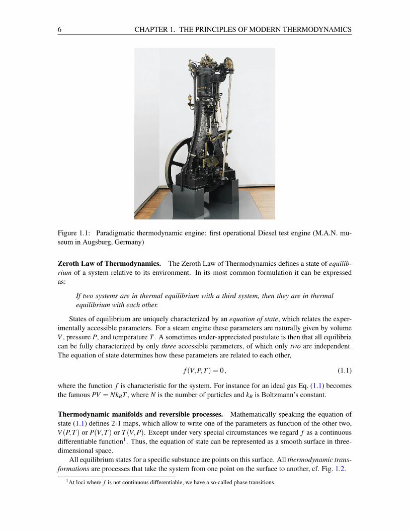
In reality, steam engines are messy, stinky, and huge [cf Fig. 1.1], which makes any attempt ofdescribing their properties from a microscopic theory futile. Thermodynamics takes a very differentperspective: rather than trying to understand all the nitty-gritty details, let’s focus on the overall,average behavior once the engine is running smoothly – once it has reached its stationary state ofoperation.
1.1.1 The five laws of thermodynamics
The framework of thermodynamics is built upon five laws, which axiomatically paraphrase ordinaryexperience and observation of nature. The central notion is equilibrium, and the central focus is ontransformations of systems from one state of equilibrium to another.
5
6 CHAPTER 1. THE PRINCIPLES OF MODERN THERMODYNAMICS
Figure 1.1: Paradigmatic thermodynamic engine: first operational Diesel test engine (M.A.N. mu-seum in Augsburg, Germany)
Zeroth Law of Thermodynamics. The Zeroth Law of Thermodynamics defines a state of equilib-rium of a system relative to its environment. In its most common formulation it can be expressedas:
If two systems are in thermal equilibrium with a third system, then they are in thermalequilibrium with each other.
States of equilibrium are uniquely characterized by an equation of state, which relates the exper-imentally accessible parameters. For a steam engine these parameters are naturally given by volumeV , pressure P, and temperature T . A sometimes under-appreciated postulate is then that all equilibriacan be fully characterized by only three accessible parameters, of which only two are independent.The equation of state determines how these parameters are related to each other,
f (V,P,T ) = 0 , (1.1)
where the function f is characteristic for the system. For instance for an ideal gas Eq. (1.1) becomesthe famous PV = NkBT , where N is the number of particles and kB is Boltzmann’s constant.
Thermodynamic manifolds and reversible processes. Mathematically speaking the equation ofstate (1.1) defines 2-1 maps, which allow to write one of the parameters as function of the other two,V (P,T ) or P(V,T ) or T (V,P). Except under very special circumstances we regard f as a continuousdifferentiable function1. Thus, the equation of state can be represented as a smooth surface in three-dimensional space.
All equilibrium states for a specific substance are points on this surface. All thermodynamic trans-formations are processes that take the system from one point on the surface to another, cf. Fig. 1.2.
1At loci where f is not continuous differentiable, we have a so-called phase transitions.
1.1. A PHENOMENOLOGICAL THEORY OF HEAT AND WORK 7
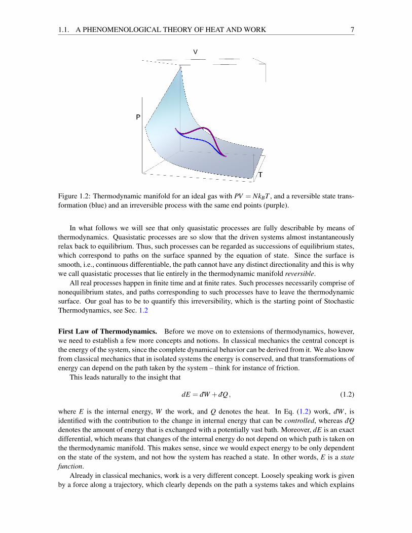
Figure 1.2: Thermodynamic manifold for an ideal gas with PV = NkBT , and a reversible state trans-formation (blue) and an irreversible process with the same end points (purple).
In what follows we will see that only quasistatic processes are fully describable by means ofthermodynamics. Quasistatic processes are so slow that the driven systems almost instantaneouslyrelax back to equilibrium. Thus, such processes can be regarded as successions of equilibrium states,which correspond to paths on the surface spanned by the equation of state. Since the surface issmooth, i.e., continuous differentiable, the path cannot have any distinct directionality and this is whywe call quasistatic processes that lie entirely in the thermodynamic manifold reversible.
All real processes happen in finite time and at finite rates. Such processes necessarily comprise ofnonequilibrium states, and paths corresponding to such processes have to leave the thermodynamicsurface. Our goal has to be to quantify this irreversibility, which is the starting point of StochasticThermodynamics, see Sec. 1.2
First Law of Thermodynamics. Before we move on to extensions of thermodynamics, however,we need to establish a few more concepts and notions. In classical mechanics the central concept isthe energy of the system, since the complete dynamical behavior can be derived from it. We also knowfrom classical mechanics that in isolated systems the energy is conserved, and that transformations ofenergy can depend on the path taken by the system – think for instance of friction.
This leads naturally to the insight that
dE = dW + dQ , (1.2)
where E is the internal energy, W the work, and Q denotes the heat. In Eq. (1.2) work, dW , isidentified with the contribution to the change in internal energy that can be controlled, whereas dQdenotes the amount of energy that is exchanged with a potentially vast bath. Moreover, dE is an exactdifferential, which means that changes of the internal energy do not depend on which path is taken onthe thermodynamic manifold. This makes sense, since we would expect energy to be only dependenton the state of the system, and not how the system has reached a state. In other words, E is a statefunction.
Already in classical mechanics, work is a very different concept. Loosely speaking work is givenby a force along a trajectory, which clearly depends on the path a systems takes and which explains
8 CHAPTER 1. THE PRINCIPLES OF MODERN THERMODYNAMICS
Rudolf J. E. Clausius:... as I hold it better to borrow terms for important mag-nitudes from the ancient languages, so that they may beadopted unchanged in all modern languages, I proposeto call [it] the entropy of the body, from the Greek word“trope for “transformation” I have intentionally formedthe word “entropy to be as similar as possible to theword “energy”; for the two magnitudes to be denoted bythese words are so nearly allied in their physical mean-ings, that a certain similarity in designation appears tobe desirable [4].
why dW is a non-exact differential. We can further identify infinitesimal changes in work as
dW =−PdV , (1.3)
which is fully analogous to classical mechanics. The other quantity, the one that quantifies the uselesschange of internal energy, the part that is typically wasted into the environment, the heat Q hasno equivalent in classical mechanics. It is rather characterized and specified by the second law ofthermodynamics.
Second Law of Thermodynamics. Let us inspect the first law of thermodynamics as expressed inEq. (1.2). If dE is an exact differential, and dW is a non-exact differential, then dQ also has to benon-exact. However, it is relatively simple to understand from its definition how dW can be writtenin terms of an exact differential. It is the force that depends in the path taken, yet the path length hasto be an exact differential – if you walk a closed loop you return to your point of origin with certainty.
Finding the corresponding exact differential, i.e., the line element for dQ was a rather challengingtask. A first account goes back to Clausius who realized [4] that∮ dQ
T≤ 0 (1.4)
where T is the temperature of the substance undergoing the cyclic, thermodynamic transformation.Moreover, the inequality in Eq. (1.4) becomes an equality for quasistatic processes. Thus, it seemsnatural to define a new state function, S, for reversible processes through
dS≡ dQT
. (1.5)
and that is known as thermodynamic entropy.To get a better understanding of this quantity consider a thermodynamic process that takes a
system from a point A on the thermodynamic manifold to a point B. Now imagine that the system istaken from A to B along a reversible path, and it returns from B to A along an irreversible path. Forsuch a cycle, the latter two equations give combined,
∆SA→B ≥∫ B
A
dQT
, (1.6)
which is known as Clausius inequality.
1.1. A PHENOMENOLOGICAL THEORY OF HEAT AND WORK 9
The Clausius inequality (1.6) is an expression of the second law of thermodynamics. More gen-erally, the second law is a collection of statements that at their core express that the entropy of theUniverse is a non-decreasing function of time,
∆SUniverse ≥ 0 . (1.7)
The most prominent, and also the oldest expressions of the second law of thermodynamics are for-mulated in terms of cyclic processes. The Kelvin-Planck statement asserts that
no process is possible whose sole result is the extraction of energy from a heat bath, andthe conversion of all that energy into work.
The Clausius statement reads,
no process is possible whose sole result is the transfer of heat from a body of lowertemperature to a body of higher temperature.
Finally, the Carnot statement declares that
no engine operating between two heat reservoirs can be more efficient than a Carnotengine operating between those same reservoirs.
These formulations refer to processes involving the exchange of energy among idealized subsystems:one or more heat reservoirs; a work source – for example, a mass that can be raised or loweredagainst gravity; and a device that operates in cycles and affects the transfer of energy among theother subsystems. All three statements follow from simple entropy-balance analyzes and offer useful,logically transparent reference points as one navigates the application of the laws of thermodynamicsto real systems.
Third Law of Thermodynamics. The Third Law of Thermodynamics or the Nernst Theorem para-phrases that in classical systems the entropy vanishes in the limit of T → 0. A little more precisely,the Nernst theorem states that as absolute zero of the temperature is approached, the entropy change∆S for a chemical or physical transformation approaches 0,
limT→0
∆S = 0 (1.8)
It is interesting to note that this equation is a modern statement of the theorem. Nernst often used aform that avoided the concept of entropy, since, e.g., for quantum mechanical systems the validity ofEq. (1.8) is somewhat questionable.
Fourth Law of Thermodynamics. The fourth law of thermodynamics takes the first step awayfrom a mere equilibrium theory. In reality, few systems can ever be found in isotropic and homoge-neous states of equilibrium. Rather, physical properties vary as functions of space~r and time t.
Nevertheless, it is frequently not such a bad approximation to assume that a thermodynamicsystem is in a state of local equilibrium. This means that for any point in space and time, the systemappears to be in equilibrium, yet thermodynamic properties vary weakly on macroscopic scales. Insuch situations we can introduce the local temperature, T (~r, t), the local density, n(~r, t), and the localenergy density, e(~r, t). The question now is, what general and universal statements can be made aboutthe resulting transport driven by local gradients of the thermodynamic variables.
10 CHAPTER 1. THE PRINCIPLES OF MODERN THERMODYNAMICS
The clearest picture arises if we look at the dynamics of the local entropy, s(~r, t). We can write
dsdt
= ∑k
∂ s∂Xk
dXk
dt, (1.9)
where Xkk is a set of extensive parameters that vary as a function of time. The time-derivative ofthese Xk define the thermodynamic fluxes
Jk ≡dXk
dt(1.10)
and the variation of the entropy as a function of the Xk are the thermodynamic forces or affinities, Fk.In short, we have
dsdt
= ∑k
FkJk . (1.11)
This means that the rate of entropy production is the sum of products of each flux with its associatedaffinity.
It should not come as a surprise that Eq. (1.11) is conceptually interesting, but practically ofrather limited applicability. The problem is that generally the fluxes are complicated functions of allforces and local gradients, Jk(F0,F1, . . .). A simplifying case is purely resistive systems, for which bydefinition the local flux only depends on the instantaneous local affinities. For small affinities, i.e., ifthe systems is in local equilibrium, Jk can be expanded in Fk. In leading order we have,
Jk = ∑j
L j,kFj , (1.12)
where the kinetic coefficients L j,k are given by
L j,k ≡∂Jk
∂Fj
∣∣∣∣Fj=0
, (1.13)
with Fj = 0 in equilibrium.The Onsager theorem [39], which is also known as the Fourth Law of Thermodynamics, now
statesL j,k = Lk, j . (1.14)
This means that the matrix of kinetic coefficients is symmetric. Therefore, to a certain degreeEq. (1.14) is a thermodynamic equivalent of Newton’s third law. This analogy becomes even clearerif we interpret Eq. (1.12) as a thermodynamic equivalent of Newton’s second law.
It is interesting to consider when the above considerations break down. Throughout this littleexercise we have explicitly assumed that the considered system is in a state of local equilibrium.This is justified as long as the flux and affinities are small. Consider, for instance, a system with atemperature gradient. For small temperature differences the flow is laminar, and the Onsager theorem(1.14) is expected hold. For large temperature differences the flow becomes turbulent, and the fluxescan no longer be balanced.
1.1.2 Finite-time thermodynamics and endoreversibility
A standard exercise in thermodynamics is to compute the efficiency of cycles, i.e., to determine therelative work output for devices undergoing cyclic transformations on the thermodynamic manifold.However, all standard cycles, such as the Carnot, Otto, Diesel, etc. cycles have in common that theyare comprised of only quasistatic state transformations, and hence their power output is strictly zero.
1.1. A PHENOMENOLOGICAL THEORY OF HEAT AND WORK 11
Lars Onsager:Now if we look at the condition of detailed balancingfrom the thermodynamic point of view, it is quite analo-gous to the principle of least dissipation [40].
This insight led Curzon and Ahlborn to ask a slightly different, yet a lot more practical question[8]: “What is the efficiency of a Carnot engine at maximal power output?” Obviously such a cyclecan no longer be reversible, but we still would like to be able to use the methods and notions fromthermodynamics. This is possible if one takes the aforementioned idea of local equilibrium one stepfurther.
Imagine a device, whose working medium is in thermal equilibrium at temperature Tw, but thereis a temperature gradient over its boundaries to the environment at temperature T . A typical exampleis a not perfectly insulating thermo-can. Now let us now imagine that the device is slowly driventhrough a cycle, where slow means that the working medium remains in a local equilibrium state atall instants. However, we will also assume that the cycle operates too fast for the working medium toever equilibrate with the environment, and thus from the point of view of the environment the deviceundergoes an irreversible cycle. Such state transformations are called endoreversible, which meansthat locally the transformation is reversible, but globally irreversible.
This idea can then be applied to the Carnot cycle, and we can determine its endoreversible ef-ficiency. The standard Carnot cycle consists of two isothermal processes during which the systemsabsorbs/exhausts heat and two thermodynamically adiabatic, i.e., isentropic strokes. Since the work-ing medium is not in equilibrium with the environment, we will have to modify the treatment of theisothermal strokes. The adiabatic strokes constitute no exchange of heat, and thus they do not need tobe re-considered.
During the hot isotherm the working medium is assumed to be a little cooler than the environment.Thus, during the whole stroke the system absorbs the heat
Qh = κhτh (Th−Thw) , (1.15)
where τh is the time the isotherm needs to complete and κh is a constant depending on thicknessand thermal conductivity of the boundary separating working medium and environment. Note thatEq. (1.15) is nothing else but a discretized version of Fourier’s law for heat conduction.
Similarly, during the cold isotherm the system is a little warmer than the cold reservoir. Hencethe exhausted heat becomes
Qc = κcτc (Tcw−Tc) (1.16)
where κc is the heat transfer coefficient for the cold reservoir.As mentioned above, the adiabatic strokes are unmodified, but we note that the cycle is taken to
be reversible with respect to the local temperatures of the working medium. Hence, we can write
∆Sh =−∆Sc and thusQh
Thw=
Qc
Tcw. (1.17)
12 CHAPTER 1. THE PRINCIPLES OF MODERN THERMODYNAMICS
The latter will be useful to relate the stroke times τh and τc to the heat transfer coefficients κh and κc.We are now interested in determining the efficiency at maximal power. To this end, we write the
power output of the cycle as
P(δTh,δTc) =Qh−Qc
ζ (τh + τc)(1.18)
where δTh = Th−Thw and δTc = Tcw−Tc. In Eq. (1.18) we introduced the total cycle time ζ (τh+τc).This means we suppress any explicit dependence of the analysis on the lengths of the adiabatic strokesand exclusively focus on the isotherms, i.e, on the temperature difference between working mediumand the hot and cold reservoirs.
It is then a simple exercise to find the maximum of P(δTh,δTc) as a function of δTh and δTc.After a few lines of algebra one obtains [8]
Pmax =κhκc
ζ
(√Th−√
Tc√κh +
√κc
)2
, (1.19)
where the maximum is assumed for
δTh
Th=
1−√
Tc/Th
1+√
κh/κcand
δTc
Tc=
√Th/Tc−1
1+√
κc/κh(1.20)
From these expressions we can now compute the efficiency. We have,
η =Qh−Qc
Qh= 1− Tcw
Thw= 1− Tc +δTc
Th−δTh(1.21)
where we used Eq. (1.17). Thus, the efficiency of an endoreversible Carnot cycle at maximal poweroutput is given by
ηCA = 1−√
Tc
Th, (1.22)
which only depends on the temperatures of the hot and cold reservoirs.The Curzon-Ahlborn efficiency is one of the first results that illustrate that (i) thermodynamics can
be extended to treat nonequilibrium systems, and that (ii) also far from thermal equilibrium universaland mathematically simple relations govern the thermodynamic behavior. In the following we willanalyze this observation a little more closely and see how universal statements arise from the natureof fluctuations.
1.2 The advent of Stochastic Thermodynamics
Relatively recently, Evans and co-workers [5] discovered an unexpected symmetry in the simulationof sheared fluids. In small systems the dynamics is governed by thermal fluctuations and, thus, alsothermodynamic quantities such as heat and work fluctuate. Remarkably, single fluctuations can be atvariance with the macroscopic statements of the second law. For instance, the change of entropy canbe negative, or the performed work amounts to less than the free energy difference. Nevertheless, theprobability distribution for the thermodynamic observables fulfills a symmetry relation, which hasbecome known as fluctuation theorem.
In its most general form the fluctuation theorem relates the probability to find a negative entropyproduction Σ with the probability of the positive value,
P (Σ =−A)P (Σ = A)
= exp(−A) . (1.23)
1.2. THE ADVENT OF STOCHASTIC THERMODYNAMICS 13
Using Jensen’s inequality for exponentials, exp(−〈x〉)≥ 〈exp(−x)〉, Eq. (1.23), immediately impliesthat
〈Σ〉 ≥ 0 , (1.24)
which is a variation of the Clausius inequality Eq. (1.6). Therefore, the fluctuation theorem canbe interpreted as a generalization of the second law to systems far from equilibrium. For the averageentropy production we retrieve the “old” statements. However, we also have that negative fluctuationsof the entropy production do occur – they are just exponentially unlikely.
The first rigorous proof of the fluctuation theorem was published by Gallavotti and Cohen in 1995[17], which was quickly generalized to Langevin dynamics [32] and general Markov processes [35].
The discovery of the fluctuation theorems has effectively opened a new area of thermodynamics,which adopted the name Stochastic Thermodynamics. Rather than focusing on describing macro-scopic systems in equilibrium, Stochastic Thermodynamics is interested in the thermodynamic be-havior of small systems that operate far from thermal equilibrium and whose dynamics are governedby fluctuations. Since quantum systems obviously fall into this class, we will briefly summarize themajor achievements for classical systems that laid the ground work for what we will eventually beinterested in – the thermodynamics of quantum systems.
1.2.1 Microscopic dynamics
To fully understand and appreciate the fluctuation theorem Eq. (1.23) we continue by briefly outliningthe most important descriptions of random motion. Generally there are two distinct approaches: (i)explicitly modeling the dynamics of a stochastic observable, or (ii) describing the dynamics of theprobability density function of a stochastic variable. Among the many variations of these two ap-proaches the conceptually simplest notions are the Langevin equation and the Klein-Kramers equa-tion.
Langevin equation. In 1908 Paul Langevin, a French physicist, proposed a powerful descriptionof Brownian motion [34, 36]. The Langevin equation is a Newtonian equation of motion for a singleBrownian particle driven by a stochastic force modeling the random kicks from the environment,
mx+mγ x+V ′(x) = ξ (t) . (1.25)
Here, m denotes the mass of the particle, γ is the damping coefficient and V ′(x) = ∂x V (x) is a con-servative force from a confining potential. The stochastic force, ξ (t) describes the randomness ina small, but open system due to thermal fluctuations. In the simplest case, ξ (t) is assumed to beGaussian white noise, which is characterized by,
〈ξ (t)〉= 0 and 〈ξ (t)ξ (s)〉= 2Dδ (t− s) , (1.26)
where D is the diffusion coefficient. Despite its apparently simple form the Langevin equation (1.25)exhibits several mathematical peculiarities. How to properly handle the stochastic force, ξ (t), led tothe study of stochastic differential equations, for which we refer to the literature [45].
It is interesting to note that the Langevin equation (1.25) is equivalent to Einstein’s treatment ofBrownian motion [15]. This can be seen by explicitly deriving the Fluctuation-Dissipation theoremfrom Eq. (1.25).
14 CHAPTER 1. THE PRINCIPLES OF MODERN THERMODYNAMICS
Fluctuation-Dissipation Theorem. The Langevin equation (1.25) for the case of a free particle,V (x) = 0, can be expressed in terms of the velocity v = x as,
mv+mγ v = ξ (t) . (1.27)
The solution of the latter first-order differential equation (1.27) reads,
vt = v0 exp(−γt)+1m
t∫0
dsξ (s) exp(−γ (t− s)) , (1.28)
where v0 is the initial velocity. Since the Langevin force is of vanishing mean (1.26), the averagedsolution 〈vt〉 becomes,
〈vt〉= v0 exp(−γt) . (1.29)
Moreover, we obtain for the mean-square velocity⟨v2
t⟩,
⟨v2
t⟩= v2
0 exp(−2γt)+1
m2
t∫0
ds1
t∫0
ds2 exp(−γ (t− s1))exp(−γ (t− s2))〈ξ (s1)ξ (s2)〉 . (1.30)
With the help of the correlation function (1.26) the twofold integral can be written in closed form and,thus, Eq. (1.30) becomes,
⟨v2
t⟩= v2
0 exp(−2γt)+D
γm2 (1− exp(−2γt)) . (1.31)
In the stationary state for γ t 1, the exponentials become negligible and the mean-square velocity(1.31) further simplifies to, ⟨
v2t⟩=
Dγm2 . (1.32)
However, we also know from kinetic gas theory [2] that in equilibrium⟨v2
t⟩= 1/βm where we
introduce the inverse temperature, β = 1/kBT . Thus, we finally have
D =mγ
β, (1.33)
which is the Fluctuation-Dissipation Theorem.
Klein-Kramers equation. The Klein-Kramers equation is an equation of motion for distributionfunctions in position and velocity space, which is equivalent to the Langevin equation (1.25), seealso [45]. For a Brownian particle in one-dimension it takes the form,
∂
∂ tP(x,v, t) =− ∂
∂x(vP(x,v, t))+
∂
∂v
(V ′(x)
mP(x,v, t)+ γvP(x,v, t)
)+
γ
mβ
∂ 2
∂v2 P(x,v, t) , (1.34)
Note that by construction the stationary solution of the Klein-Kramers equation (1.34) is the Boltzmann-Gibbs distribution, Peq ∝ exp
(−β/2mv2−βV
). The main advantage of the Klein-Kramers equation
(1.34) over the Langevin equation (1.25) is that we can compute the entropy production directly,which we will exploit shortly for quantum systems in Sec. 1.4.5.
1.2. THE ADVENT OF STOCHASTIC THERMODYNAMICS 15
1.2.2 Stochastic energetics
An important step towards the discovery of the fluctuation theorems (1.23) was Sekimoto’s insightthat thermodynamic notions can be generalized to single particle dynamics [46]. To this end, considerthe overdamped Langevin equation
0 =−(−mγ x+ξt)dx+∂xV (x,λ )dx , (1.35)
where we separated contributions stemming from the interaction with the environment and mechani-cal forces. Here and in the following, λ is an external control parameter, whose variation drives thesystem.
Generally, a change in internal energy of a single particle is comprised of changes in kinetic andpotential energy. In the overdamped limit, however, one assumes that the momentum degrees offreedom equilibrate much faster than any other time-scale of the dynamics. Thus, the kinetic energyis always at its equilibrium value, and thus a change in internal energy, de, for a single trajectory, x,is given by
de(x,λ ) = dV (x,λ ) = ∂xV (x,λ )dx+∂λV (x,λ )dλ . (1.36)
Further, identifying the heat with the external terms in Eq. (1.35), which are governed by the dampingand the noise, we can write
dq(x) = (−mγ x+ξt)dx . (1.37)
Thus, we obtain a stochastic, microscopic expression of the first law (1.2)
0 =−dq(x)+de(x,λ )−∂λV (x,λ )dλ , (1.38)
which uniquely defines the stochastic work for a single trajectory,
dw(x) = ∂λV (x,λ )dλ (1.39)
Note that the work increment, dw, is given by the partial derivative of the potential with respect to theexternally controllable work parameter, λ .
1.2.3 Jarzynski equality and Crooks theorem
The stochastic work increment dw(x) uniquely characterizes the thermodynamics of single Brownianparticles. However, since dw(x) is subject to thermal fluctuations none of the traditional statementsof the second law can be directly applied, and in particular there is no maximum work theorem fordw(x). Therefore, special interest has to be on the distribution of P(W ), where W =
∫dw(x) is the
accumulated work performed during a thermodynamic process.In the following we will briefly discuss representative derivations of the most prominent fluctua-
tion theorems, namely the classical Jarzynski equality and the Crooks theorem, and then the quantumJarzynski equality in Sec. 1.4.3 and finally a quantum fluctuation theorem for entropy production inSec. 1.4.5.
Jarzynski equality. Thermodynamically, the simplest cases are systems that are isolated from theirthermal environment. Realistically imagine, for instance, a small system that is ultraweakly coupledto the environment. If left alone, the system equilibrates at inverse temperature β for a fixed workparameter, λ . Then, the time scale of the variation of the work parameter is taken to be much shorterthan the relaxation time, 1/γ . Hence, the dynamics of the system during the variation of λ can beapproximated by Hamilton’s equations of motion to high accuracy.
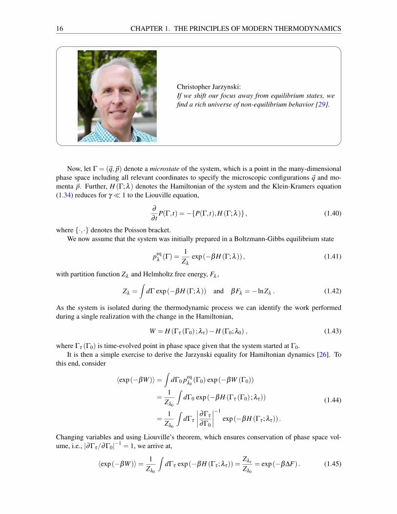
16 CHAPTER 1. THE PRINCIPLES OF MODERN THERMODYNAMICS
Christopher Jarzynski:If we shift our focus away from equilibrium states, wefind a rich universe of non-equilibrium behavior [29].
Now, let Γ = (~q,~p) denote a microstate of the system, which is a point in the many-dimensionalphase space including all relevant coordinates to specify the microscopic configurations ~q and mo-menta ~p. Further, H (Γ;λ ) denotes the Hamiltonian of the system and the Klein-Kramers equation(1.34) reduces for γ 1 to the Liouville equation,
∂
∂ tP(Γ, t) =−P(Γ, t),H (Γ;λ ) , (1.40)
where ·, · denotes the Poisson bracket.We now assume that the system was initially prepared in a Boltzmann-Gibbs equilibrium state
peqλ(Γ) =
1Zλ
exp(−βH (Γ;λ )) , (1.41)
with partition function Zλ and Helmholtz free energy, Fλ ,
Zλ =∫
dΓ exp(−βH (Γ;λ )) and βFλ =− lnZλ . (1.42)
As the system is isolated during the thermodynamic process we can identify the work performedduring a single realization with the change in the Hamiltonian,
W = H (Γτ (Γ0) ;λτ)−H (Γ0;λ0) , (1.43)
where Γτ (Γ0) is time-evolved point in phase space given that the system started at Γ0.It is then a simple exercise to derive the Jarzynski equality for Hamiltonian dynamics [26]. To
this end, consider
〈exp(−βW )〉=∫
dΓ0 peqλ0(Γ0) exp(−βW (Γ0))
=1
Zλ0
∫dΓ0 exp(−βH (Γτ (Γ0) ;λτ))
=1
Zλ0
∫dΓτ
∣∣∣∣∂Γτ
∂Γ0
∣∣∣∣−1
exp(−βH (Γτ ;λτ)) .
(1.44)
Changing variables and using Liouville’s theorem, which ensures conservation of phase space vol-ume, i.e., |∂Γτ/∂Γ0|−1 = 1, we arrive at,
〈exp(−βW )〉= 1Zλ0
∫dΓτ exp(−βH (Γτ ;λτ)) =
Zλτ
Zλ0
= exp(−β∆F) . (1.45)
1.2. THE ADVENT OF STOCHASTIC THERMODYNAMICS 17
The Jarzynski equality (1.45) is one of the most important building blocks of modern thermody-namics [41]. It can be rightly understood as a generalization of the second law of thermodynamics tosystems far from equilibrium, and it has been shown to hold a in wide range of classical systems, withweak and strong coupling, with slow and fast dynamics, with Markovian and non-Markovian noiseetc. [28].
Crooks’s fluctuation theorem. The second most prominent fluctuation theorem is the work relationby Crooks [6, 7]. As before we are interested in the evolution of a thermodynamic system for times0≤ t ≤ τ , during which the work parameter, λt , is varied according to some protocol. For the presentpurposes, we now assume that the thermodynamic process is described as a sequence, Γ0,Γ1, ...,ΓN ,of microstates visited at times t0, t1, ..., tN as the system evolves. For the sake of simplicity we assumethe time sequence to be equally distributed, tn = nτ/N, and, implicitly, (ΓN ; tN) = (Γτ ;τ). Moreover,we assume that the evolution is a Markov process: given the microstate Γn at time tn, the subsequentmicrostate Γn+1 is sampled randomly from a transition probability distribution, P, that depends merelyon Γn, but not on the microstates visited at earlier times than tn [54]. This means that the transitionprobability to go from Γn to Γn+1 depends only on the current microstate, Γn, and the the currentvalue of the work parameter, λn. Finally, we assume that the system fulfills a local detailed balancecondition [54], namely
P(Γ→ Γ′;λ )
P(Γ← Γ′;λ )=
exp(−βH (Γ′;λ ))
exp(−βH (Γ;λ )). (1.46)
When the work parameter, λ , is varied in discrete time steps from λ0 to λN = λτ , the evolution ofthe system during one time step can be expressed as a sequence,
forward : (Γn,λn)→ (Γn,λn+1)→ (Γn+1,λn+1) . (1.47)
In this sequence first the value of the work parameter is updated and, then, a random step is takenby the system. A trajectory of the whole process between initial, Γ0, and final microstate, Γτ , isgenerated by first sampling Γ0 from the initial, Boltzmann-Gibbs distribution peq
λ0and, then, repeating
Eq. (1.47) in time increments, δ t = τ/N.Consequently, the net change in internal energy, ∆E = H (ΓN ,λN)−H (Γ0,λ0), can be written as
a sum of two contributions. First, the changes in energy due to variations of the work parameter,
W =N−1
∑n=0
[H (Γn;λn+1)−H (Γn;λn)] , (1.48)
and second, changes due to transitions between microstates in phase space,
Q =N−1
∑n=0
[H (Γn+1;λn+1)−H (Γn;λn+1)] . (1.49)
As argued by Crooks [6] the first contribution (1.48) is given by an internal change in energy and thesecond term (1.49) stems from the interaction with the environment introducing the random steps inphase space. Thus, Eq. (1.48) is a natural definition of stochastic work, and Eq. (1.49) is the stochasticheat for a single trajectory.
The probability to generate a trajectory, Ξ = (Γ0→ ...ΓN), starting in a particular initial state, Γ0,is given by the product of the initial distribution and all subsequent transition probabilities,
PF [Ξ] = peqλ0(Γ0)
N−1
∏n=0
P(Γn→ Γn+1;λn+1) , (1.50)
18 CHAPTER 1. THE PRINCIPLES OF MODERN THERMODYNAMICS
where the stochastic independency of the single steps is guaranteed by the Markov assumption.Analogously to the forward process, we can define a reverse trajectory with (λ0← λτ). However,
the starting point is sampled from peqλτ
and the system first takes a random step and, then, the value ofthe work parameter is updated,
reversed : (Γn+1,λn+1)← (Γn+1,λn)← (Γn,λn) . (1.51)
Now, we compare the probability of a trajectory Ξ during a forward process, PF [Ξ], with the proba-bility of the conjugated path, Ξ† = (Γ0← ...ΓN), during the reversed process, PR[Ξ†]. The ratio ofthese probabilities reads,
PF [Ξ]
PR[Ξ†]=
peqλ0(Γ0)
N−1∏
n=0P(Γn→ Γn+1;λ F
n+1)
peqλ1(ΓN)
N−1∏
n=0P(Γn← Γn+1;λ R
N−1−n
) . (1.52)
Here,
λ F0 ,λ F
1 , ...,λ FN
is the protocol for varying the external work parameter from λ0 to λτ duringthe forward process. Analogously,
λ R
0 ,λR1 , ...,λ
RN
specifies the reversed process, which is related tothe forward process by,
λRn = λ
FN−n . (1.53)
Hence, every factor P(Γ→ Γ′;λ ) in the numerator of the ratio (1.52) is matched by P(Γ← Γ′;λ ) inthe denominator.
In conclusion, Eq. (1.52) reduces to [6],
PF [Ξ]
PR[Ξ†]= exp
(β(W F [Ξ]−∆F
)), (1.54)
where W F [Ξ] is the work performed on the system during the forward process.Forward work, W F [Ξ], and reverse work, W R[Ξ†], are related through
W F [Ξ] =−W R[Ξ†] (1.55)
for a conjugate pair of trajectories, Ξ and Ξ†. The corresponding work distributions, PF and PR, arethen given by an average over all possible realizations, i.e. all discrete trajectories of the process,
PF (+W ) =∫
dΞPF [Ξ]δ(W −W F [Ξ]
)PR (−W ) =
∫dΞPR[Ξ†]δ
(W +W R[Ξ†]
),
(1.56)
where dΞ = dΞ† = ∏n dΓn. Collecting Eqs. (1.54) and (1.56) the work distribution for the forwardprocesses can be written as
PF (+W ) = exp(β (W −∆F))∫
dΞPR[Ξ†]δ(W +W R[Ξ†]
), (1.57)
from which we obtain the Crooks fluctuation theorem [7]
PR (−W ) = exp(−β (W −∆F))PF (+W ) . (1.58)
It is interesting to note that the Crooks theorem (1.58) is a detailed version of the Jarzynskiequality (1.45), which follows from integrating Eq. (1.58) over the forward work distribution,
1 =∫
dW PR (−W ) =∫
dW exp(−β (W −∆F))PF (+W ) = 〈exp(−β (W −∆F))〉F . (1.59)
Note, however, that the Crooks theorem (1.58) is only valid for Markovian processes [27], whereasthe Jarzynski equality can also be shown to hold for non-Markovian dynamics [48].
1.3. FOUNDATIONS OF STATISTICAL PHYSICS FROM QUANTUM ENTANGLEMENT 19
1.3 Foundations of statistical physics from quantum entanglement
In the preceding section we implicitly assumed that there is a well-established theory if and howphysical systems are described in a state of thermal equilibrium. For instance, in the treatment ofthe Jarzynski equality (1.45) and the Crooks fluctuation theorem (1.58) we assumed that the systemis initially prepared in a Boltzmann-Gibbs distribution. In standard textbooks of statistical physicsthis description of canonical thermal equilibria is usually derived from the fundamental postulate,Boltzmann’s H-theorem, the ergodic hypothesis, or the maximization of the statistical entropy inequilibrium [2, 52]. However, none of these concepts are particularly well-phrased for quantum sys-tems.
It is important to realize that statistical physics was developed in the XIX century, when the fun-damental physical theory was classical mechanics. Statistical physics was then developed to translatebetween microstates (points in phase space) and thermodynamic macrostates (given by temperature,entropy, pressure, etc). Since microstates and macrostates are very different notions a new theorybecame necessary that allows to “translate” with the help of fictitious, but useful, concepts such asensembles. However, ensembles consisting of infinitely many copies of the same system seem ratherill-defined from the point of view of a fully quantum theory.
Only relatively recently this conceptual problem was repaired by showing that the famous repre-sentations of microcanonical and canonical equilibria can be obtained from a fully quantum treatment– from symmetry considerations of entanglement [13]. This novel approach to the foundations of sta-tistical mechanics relies on entanglement assisted invariance or in short on envariance [59–61].
In the following we summarize the main conceptual steps that were originally published inRef. [13].
1.3.1 Entanglement assisted invariance
Consider a quantum system, S , which is maximally entangled with an environment, E , and let|ψS E 〉 denote the composite state in S ⊗E . Then |ψS E 〉 is called envariant under a unitary mapUS = uS ⊗ IE if and only if there exists another unitary UE = IS ⊗uE such that,
US |ψS E 〉= (uS ⊗ IE ) |ψS E 〉= |ηS E 〉UE |ηS E 〉= (IS ⊗uE ) |ηS E 〉= |ψS E 〉 .
(1.60)
Thus, UE that does not act on S “does the job” of the inverse map of US on S – assisted by theenvironment E .
The principle is most easily illustrated with a simple example. Suppose S and E are each givenby two-level systems, where |↑〉S , |↓〉S are the eigenstates of S and |↑〉E , |↓〉E span E . Now,further assume |ψS E 〉∝ |↑〉S ⊗|↑〉E + |↓〉S ⊗|↓〉E and US is a swap in S – it “flips” its spin. Then,we have
|↑〉S⊗|↑〉E+|↓〉S⊗|↓〉EUS−−−−−→ |↓〉S ⊗|↑〉E + |↑〉S ⊗|↓〉E . (1.61)
The action of US on |ψ〉S E can be restored by a swap, UE , on E ,
|↓〉S⊗|↑〉E+|↑〉S⊗|↓〉EUE−−−−−→ |↓〉S ⊗|↓〉E + |↑〉S ⊗|↑〉E . (1.62)
20 CHAPTER 1. THE PRINCIPLES OF MODERN THERMODYNAMICS
Thus, the swap UE on E restores the pre-swap |ψ〉S E without “touching” S , i.e., the global stateis restored by solely acting on E . Consequently, local probabilities of the two swapped spin statesare both exchanged and unchanged. Hence, they have to be equal. This provides the fundamentalconnection of quantum states and probabilities [59], and leads to Born’s rule [60].
Recent experiments in quantum optics [23, 56] and on IBM’s Q Experience [10] have shownthat envariance is not only a theoretical concept, but a physical reality. Thus, envariance is a validand purely quantum mechanical concept that we can use as a stepping stone to motivate and derivequantum representations of thermodynamic equilibrium states.
1.3.2 Microcanonical state from envariance
We begin by considering the microcanonical equilibrium. Generally, thermodynamic equilibriumstates are characterized by extrema of physical properties, such as maximal phase space volume,maximal thermodynamic entropy, or maximal randomness [53]. We will define the microcanoni-cal equilibrium as the quantum state that is “maximally envariant”, i.e., envariant under all unitaryoperations on S . To this end, we write the composite state |ψS E 〉 in Schmidt decomposition [38],
|ψS E 〉= ∑k
ak |sk〉⊗ |εk〉 , (1.63)
where by definition |sk〉 and |εk〉 are orthocomplete in S and E , respectively. The task is now toidentify the “special” state that is maximally envariant.
It has been shown [60] that |ψS E 〉 is envariant under all unitary operations if and only if theSchmidt decomposition is even, i.e., all coefficients have the same absolute value, |ak|= |al| for all land k. We then can write,
|ψS E 〉 ∝ ∑k
exp(iφk) |sk〉⊗ |εk〉 , (1.64)
where φk are phases. Recall that in classical statistical mechanics equilibrium ensembles are identifiedas the states with the largest corresponding volume in phase space [53]. In the present context this“identification” readily translates into an equilibrium state that is envariant under the maximal numberof, i.e., all unitary operations.
To conclude the derivation we note that the microcanonical state is commonly identified as thestate that is also fully energetically degenerate [2]. To this end, denote the Hamiltonian of the com-posite system by
HS E = H⊗ IE + IS ⊗HE . (1.65)
Then, the internal energy of S is given by the quantum mechanical average
E = 〈ψS E |(H⊗ IE ) |ψS E 〉= ∑k〈sk|H |sk〉/Zmic , (1.66)
where Zmic is the energy-dependent dimension of the Hilbert space of S , which is commonly alsocalled the microcanonical partition function [2]. Since |ψS E 〉 (1.66) is envariant under all unitarymaps we can assume without loss of generality that skZmic
k=1 is a representation of the energy eigen-basis corresponding to H, and we have 〈sk|H |sk〉= ek with E = ek = ek′ for all k,k′ ∈ 1, . . . ,Zmic.
Therefore, we have identified the fully quantum mechanical representation of the microcanonicalstate by two conditions. Note that in our framework the microcanonical equilibrium is not representedby a unique state, but rather by an equivalence class of all maximally envariant states with the sameenergy: the state representing the microcanonical equilibrium of a system S with Hamiltonian H isthe state that is (i) envariant under all unitary operations on S and (ii) fully energetically degeneratewith respect to H.
1.3. FOUNDATIONS OF STATISTICAL PHYSICS FROM QUANTUM ENTANGLEMENT 21
Reformulation of the fundamental statement. Before we continue to rebuild the foundations ofstatistical mechanics using envariance, let us briefly summarize and highlight what we have achievedso far. All standard treatments of the microcanonical state relied on notions such as probability,ergodicity, ensemble, randomness, indifference, etc. However, in the context of (quantum) statisticalphysics none of these expressions are fully well-defined. Indeed, in the early days of statistical physicsseminal researchers such as Maxwell and Boltzmann struggled with the conceptual difficulties [53].Modern interpretation and understanding of statistical mechanics, however, was invented by Gibbs,who simply ignored such foundational issues and made full use of the concept of probability.
In contrast, in this approach we only need a quantum symmetry induced by entanglement – en-variance – instead of relying on mathematically ambiguous concepts. Thus, we can reformulate thefundamental statement of statistical mechanics in quantum physics:
The microcanonical equilibrium of a system S with Hamiltonian H is a fully energeti-cally degenerate quantum state envariant under all unitaries.
We will further illustrate this fully quantum mechanical approach to the foundations of statisticalmechanics by also treating the canonical equilibrium.
1.3.3 Canonical state from quantum envariance
Let us now imagine that we can separate the total system S into a smaller subsystem of interest Sand its complement, which we call heat bath B. The Hamiltonian of S can then be written as
H = HS⊗ IB+ IS⊗HB+hS,B , (1.67)
where hS,B denotes an interaction term. Physically this term is necessary to facilitate exchange ofenergy between the S and the heat bath B. In the following, however, we will assume that hS,B issufficiently small so that we can neglect its contribution to the total energy, E =ES+EB, and its effecton the composite equilibrium state |ψS E 〉. These assumptions are in complete analogy to the ones ofclassical statistical mechanics [2, 52] and it is commonly referred to as ultraweak coupling [49].
Under these assumptions every composite energy eigenstate |sk〉 can be written as a product,
|sk〉= |sk〉⊗ |bk〉 , (1.68)
where the states |sk〉 and |bk〉 are energy eigenstates in S and B, respectively. At this point envarianceis crucial in our treatment: All orthonormal bases are equivalent under envariance. Therefore, we canchoose |sk〉 as energy eigenstates of H.
For the canonical formalism we are now interested in the number of states accessible to the totalsystem S under the condition that the total internal energy E (1.66) is given and constant. When thesubsystem of interest, S, happens to be in a particular energy eigenstate |sk〉 then the internal energyof the subsystem is given by the corresponding energy eigenvalue ek. Therefore, for the total energyE to be constant, the energy of the heat bath, EB, has to obey,
EB (ek) = E− ek . (1.69)
This condition can only be met if the energy spectrum of the heat reservoir is at least as dense as theone of the subsystem.
The number of states, N(ek), accessible to S is then given by the fraction
N(ek) =NB (E− ek)
NS (E), (1.70)
22 CHAPTER 1. THE PRINCIPLES OF MODERN THERMODYNAMICS
where NS (E) is the total number of states in S consistent with Eq. (1.66), and NB (E− ek) is thenumber of states available to the heat bath, B, determined by condition (1.69). In other words, weare asking for nothing else but the degeneracy in B corresponding to a particular energy state of thesystem of interest |sk〉.
Example: Composition of multiple qubits. The idea is most easily illustrated with a simple ex-ample, before we will derive the general formula in the following paragraph. Imagine a system ofinterest, S, that interacts with N non-interacting qubits with energy eigenstates |0〉 and |1〉 and cor-responding eigenenergies eB0 and eB1 . Note once again that the composite states |sk〉 can always bechosen to be energy eigenstates, since the even composite state |ψS E 〉 (1.64) is envariant under allunitary operations on S .
We further assume the qubits to be non-interacting. Therefore, all energy eigenstates can bewritten in the form
|sk〉= |sk〉⊗∣∣δ 1
k δ2k · · ·δ N
k⟩︸ ︷︷ ︸
N−qubits
. (1.71)
Here δ ik ∈ 0,1 for all i ∈ 1, . . . ,N describing the states of the bath qubits. Let us denote the number
of qubits of B in |0〉 by n. Then the total internal energy E becomes a simple function of n and isgiven by,
E = ek +neB0 +(N−n)eB1 . (1.72)
Now it is easy to see that the total number of states corresponding to a particular value of E, i.e., thedegeneracy in B corresponding to ek, (1.70) is given by,
N(ek) =N!
n!(N−n)!. (1.73)
Equation (1.73) describes nothing else but the number of possibilities to distribute neB0 and (N−n)eB1over N qubits.
It is worth emphasizing that in the arguments leading to Eq. (1.73) we explicitly used that the |sk〉are energy eigenstates in S and the subsystem S and heat reservoir B are non-interacting. The firstcondition is not an assumption, since the composite |ψS E 〉 is envariant under all unitary maps onS , and the second condition is in full agreement with conventional assumptions of thermodynamics[2, 52].
Boltzmann’s formula for the canonical state. The example treated in the preceding section canbe easily generalized. We again assume that the heat reservoir B consists of N non-interacting sub-systems with identical eigenvalue spectra eBj m
j=1. In this case the internal energy (1.69) takes theform
E = ek +n1 eB1 +n2 eB2 + · · ·+nmeBm , (1.74)
with ∑mj=1 n j = N. Therefore, the degeneracy (1.70) becomes
N(ek) =N!
n1!n2! · · ·nm!. (1.75)
This expression is readily recognized as a quantum envariant formulation of Boltzmann’s countingformula for the number of classical microstates [53], which quantifies the volume of phase spaceoccupied by the thermodynamic state. However, instead of having to equip phase space with an(artificial) equispaced grid, we simply count degenerate states.
1.4. WORK, HEAT, AND ENTROPY PRODUCTION 23
We are now ready to derive the Boltzmann-Gibbs formula. To this end consider that in the limitof very large, N 1, N(ek) (1.75) can be approximated with Stirling’s formula. We have
ln(N(ek))' N ln(N)−m
∑j=1
n j ln(n j) . (1.76)
As pointed out earlier, thermodynamic equilibrium states are characterized by a maximum of sym-metry or maximal number of “involved energy states”, which corresponds classically to a maximalvolume in phase space. In the case of the microcanonical equilibrium this condition was met bythe state that is maximally envariant, namely envariant under all unitary maps. Now, following Boltz-mann’s line of thought we identify the canonical equilibrium by the configuration of the heat reservoirB for which the maximal number of energy eigenvalues are occupied. Under the constraints,
m
∑j=1
n j = N and E− ek =m
∑j=1
n j eBj (1.77)
this problem can be solved by variational calculus. One obtains
n j = µ exp(
β eBj), (1.78)
which is the celebrated Boltzmann-Gibbs formula. Notice that Eq. (1.78) is the number of states inthe heat reservoir B with energy eBj for S and B being in thermodynamic, canonical equilibrium. Inthis treatment temperature merely enters through the Lagrangian multiplier β .
What remains to be shown is that β , indeed, characterizes the unique temperature of the system ofinterest, S. To this end, imagine that the total system S can be separated into two small systems S1and S2 of comparable size, and the thermal reservoir, B. It is then easy to see that the total number ofaccessible states N(ek) does not significantly change in comparison to the previous case. In particular,in the limit of an infinitely large heat bath B the total number of accessible states for B is still givenby Eq. (1.75). In addition, it can be shown that the resulting value of the Lagarange multiplier, β ,is unique [57]. Hence, we can formulate a statement of the zeroth law of thermodynamics fromenvariance – namely, two systems S1 and S2, that are in equilibrium with a large heat bath B, arealso in equilibrium with each other, and they have the same temperature corresponding to the uniquevalue of β .
The present discussion is exact, up to the approximation with the Stirling’s formula, and onlyrelies on the fact that the total system S is in a microcanonical equilibrium as defined in termsof envariance (1.68). The final derivation of the Boltzmann-Gibbs formula (1.78), however, requiresadditional thermodynamic conditions. In the case of the microcanonical equilibrium we replaced con-ventional arguments by maximal envariance, whereas for the canonical state we required the maximalnumber of energy levels of the heat reservoir to be “occupied”.
1.4 Work, heat, and entropy production
Equipped with a classical understanding of thermodynamic phenomenology, the fluctuation theorems(1.23) and understanding of equilibrium states from a fully quantum theory, we can now move on todefine work, heat, and entropy production for quantum systems. The following treatment was firstpublished in Ref. [18].
24 CHAPTER 1. THE PRINCIPLES OF MODERN THERMODYNAMICS
1.4.1 Quantum work and quantum heat
Quasistatic processes. In complete analogy to the standard framework of thermodynamics as dis-cussed in Sec. 1.1, we begin the discussion by considering quasistatic processes during which thequantum system, S , is always in equilibrium with a thermal environment. However, we now furtherassume that the Hamiltonian of the system, H(λ ), is parameterized by a control parameter λ . Theparameter can be, e.g., the volume of a piston, the angular frequency of an oscillator, the strength ofa magnetic field, etc.
Generally, the dynamics of S is then described by the Liouville type equation ρ = Lλ (ρ), wherethe superoperator Lλ reflects both the unitary dynamics generated by H and the non-unitary contri-bution induced by the interaction with the environment. We further have to assume that the equationfor the steady state, Lλ (ρ
ss) = 0, has a unique solution [49] to avoid any ambiguities. As before, wewill now be interested in thermodynamic state transformations, for which S remains in equilibriumcorresponding to the value of λ .
Thermodynamics of Gibbs equilibrium states. As we have seen above, in the the limit of ultra-weak coupling the equilibrium state is given by the Gibbs state,
ρeq = exp(−βH)/Z, where Z = trexp(−βH) , (1.79)
and where β is the inverse temperature of the environment. In this case, the thermodynamic entropyis given by the Gibbs entropy [2], S =−trρeq ln(ρeq)= β (E−F), where as before E = trρeq His the internal energy of the system, and F =−1/β ln(Z) denotes the Helmholtz free energy.
For isothermal, quasistatic processes the change of thermodynamic entropy dS can be written as
dS = β (trdρeq H+(trρeq dH−dF)) = β trdρ
eq H , (1.80)
where the second equality follows from simply evaluating terms. Therefore, two forms of energycan be identified [21]: heat is the change of internal energy associated with a change of entropy;work is the change of internal energy due to the change of an extensive parameter, i.e., change of theHamiltonian of the system. We have,
dE = dQ+ dW ≡ trdρeq H+ trρeq dH . (1.81)
The identification of heat dQ, and work dW (1.81) is consistent with the second law of thermody-namics for quasistatic processes (1.5) if, and as will shortly see, only if ρeq is a Gibbs state (1.79).
It is worth emphasizing that for isothermal, quasistatic processes we further have,
dS = β dQ and dF = dW , (1.82)
for which the first law of thermodynamics takes the form
dE = T dS+dF . (1.83)
In this particular formulation it becomes apparent that changes of the internal energy dE can beseparated into “useful” work dF and an additional contribution, T dS, reflecting the entropic cost ofthe process.
1.4. WORK, HEAT, AND ENTROPY PRODUCTION 25
Thermodynamics of non-Gibbsian equilibrium states. As we have seen above in Sec. 1.3, how-ever, quantum systems in equilibrium are only described by Gibbs states (1.79) if they are ultraweaklycoupled to the environment. Typically, quantum systems are correlated with their surroundings andinteraction energies are not negligible [20, 22, 25]. For instance, it has been seen explicitly in thecontext of quantum Brownian motion [24] that system and environment are generically entangled.
In such situations the identification of heat only with changes of the state of the system (1.81) isno longer correct [22]. Rather, to formulate thermodynamics consistently the energetic back actiondue to the correlation of system and environment has to be taken into account [22, 24]. This meansthat during quasistatic processes parts of the energy exchanged with the environment are not relatedto a change of the thermodynamic entropy of the system, but rather constitute the energetic price tomaintain the non-Gibbsian state, i.e., coherence and correlations between system and environment.
Denoting the non-Gibbsian equilibrium state by ρss we can write
H =−trρss ln(ρss)+(trρss ln(ρeq)− trρss ln(ρeq))= β [E− (F +T S(ρss||ρeq))] = β (E −F ),
(1.84)
where as before E = trρssH is the internal energy of the system, and F ≡ F +T S(ρss||ρeq) is theso-called the information free energy [42]. Further, S(ρss||ρeq) ≡ trρss (ln(ρss)− ln(ρeq)) is thequantum relative entropy [55].
In complete analogy to the standard, Gibbsian case (1.81) we now consider isothermal, quasistaticprocesses, for which the infinitesimal change of the entropy reads
dH = β [trdρssH+(trρssdH−dF )]
≡ β (dQtot− dQc) .(1.85)
where we identified the total heat as dQtot ≡ trdρssH and energetic price to maintain coherenceand quantum correlations as dQc ≡ dF − trρssdH.
The excess heat dQex is the only contribution that is associated with the entropic cost,
dH = β dQex, and dQex = dQtot− dQc . (1.86)
Accordingly, the first law of thermodynamics takes the form
dE = dWex + dQex (1.87)
where dWex≡ dW + dQc is the excess work. Finally, Eq. (1.81) generalizes for isothermal, quasistaticprocesses in generic quantum systems to
dE = T dH +dF . (1.88)
It is worth emphasizing at this point once again that thermodynamics is a phenomenological theory,and as one expects, the fundamental relations hold for any physical system. Equation (1.88) hasexactly the same form as Eq. (1.81), however, the “symbols” have to be interpreted differently whentranslating between the thermodynamic relations and the underlying statistical mechanics.
As an immediate consequence of this analysis, we can now derive the efficiency of any quantumsystem undergoing a Carnot cycle.
Universal efficiency of quantum Carnot engines. To this end, imagine a generic quantum systemthat operates between two heat reservoirs with hot, Thot, and cold, Tcold, temperatures, respectively.Then, the Carnot cycle consists of two isothermal processes during which the system absorbs/exhausts
26 CHAPTER 1. THE PRINCIPLES OF MODERN THERMODYNAMICS
heat and two thermodynamically adiabatic, i.e., isentropic strokes while the extensive control param-eter λ is varied.
During the first isothermal stroke, the system is put into contact with the hot reservoir. As a result,the excess heat Qex,1 is absorbed at temperature Thot and excess work Wex,1 is performed,
Wex,1 = F (λ2,Thot)−F (λ1,Thot)
Qex,1 = Thot (H (λ2,Thot)−H (λ1,Thot)).(1.89)
Next, during the isentropic stroke, the system performs work Wex,2 and no excess heat is exchangedwith the reservoir, ∆H = 0. Therefore, the temperature of the engine drops from Thot to Tcold,
Wex,2 = ∆E = E(λ3,Tcold)−E(λ2,Thot)
= ∆F − (Thot−Tcold) H (λ3,Tcold).(1.90)
In the second line, we employed the thermodynamic identity E = F + T H , which follows fromthe definition of F . During the second isothermal stroke, the excess work Wex,3 is performed on thesystem by the cold reservoir. This allows for the system to exhaust the excess heat Qex,3 at temperatureTcold. Hence we have
Wex,3 = F (λ4,Tcold)−F (λ3,Tcold)
Qex,3 = Tcold(H (λc,Tcold)−H (λ3,Tcold)).(1.91)
Finally, during the second isentropic stroke, the cold reservoir performs the excess work Wex,4 on thesystem. No excess heat is exchanged and the temperature of the engine increases from Tcold to Thot,
Wex,4 = ∆E = E(λ1,Thot)−E(λ4,Tcold)
= ∆F +(Thot−Tcold) H (λ1,Thot).(1.92)
The efficiency of a thermodynamic device is defined as the ratio of “output” to “input”. In thepresent case the “output” is the total work performed during each cycle, i.e., the total excess work,Wex =W +Qc. There are two physically distinct contributions: work in the usual sense, W , that can beutilized, e.g., to power external devices, and Qc, which cannot serve such purposes as it is the thermo-dynamic cost to maintain the non-Gibbsian equilibrium state. Therefore, the only thermodynamicallyconsistent definition of the efficiency is
η =∑iWex,i
Qex,1= 1− Tcold
Thot≡ ηC, (1.93)
which is identical to the classical Carnot efficiency.
1.4.2 Quantum entropy production
Having established a conceptual framework for quantum work and heat, the next natural step is todetermine the quantum entropy production. To this end, we now imagine that S is initially preparedin an equilibrium state, which however is not necessarily a Gibbs state (1.79) with respect to thetemperature of the environment. For a variation of the external control parameter λ we can write thechange of internal energy ∆E and a change of the von-Neumann entropy as
∆E =W +Q and ∆H = βQ+Σ , (1.94)
1.4. WORK, HEAT, AND ENTROPY PRODUCTION 27
where here Q is the total heat exchanged during the process with the environment at inverse tempera-ture β . Thus, we can write for the mean nonequilibrium entropy production,
Σ = ∆H −β∆E +βW . (1.95)
Now, expressing the internal energy with the help of the Gibbs state ρeq (1.79) we have
βE = β trρssH=−trρss ln(ρeq)+ ln(Z) , (1.96)
Thus, we can write for a process that varies λ from λ0 to λ1 [compare with the classical expression(1.39) and the quantum case (1.81)]
βW = β
∫λ1
λ0
dλ trρss(λ )∂λ H(λ )
=−∫
λ1
λ0
dλ trρss(λ )∂λ ln(ρeq(λ ))− ln(Z1)+ ln(Z0) .
(1.97)
Combining Eqs. (1.95)-(1.97), we obtain the general expression for the entropy production along anonequilibrium path [compare Fig. 1.2],
Σ = S (ρss(λ0)||ρeq(λ0))−S (ρss(λ1)||ρeq(λ1))−∫
λ1
λ0
dλ trρss(λ )∂λ ln(ρeq(λ )) (1.98)
Equation (1.98) is the exact microscopic expression for the mean nonequilibrium entropy productionfor a driven open quantum system weakly coupled to a single heat reservoir. It is valid for intermediatestates that can be arbitrarily far from equilibrium.
1.4.3 Two-time energy measurement approach
Having identified expressions for the average, work, heat, and entropy production, we can now con-tinue building Quantum Stochastic Thermodynamics. In complete analogy to the classical case,Quantum Stochastic Thermodynamics is built upon fluctuation theorems. Conceptually, the most in-volved problem is how to identify heat and work for single realizations – and even what a “singlerealization” means for a quantum system.
The most successful approach has become known as two-time energy measurement approach [3].In this paradigm, one considers an isolated quantum system that evolves under the time-dependentSchrodinger equation
ih∂t |ψt〉= Ht |ψt〉 . (1.99)
As before, we are interested in describing thermodynamic processes that are induced by varyingan external control parameter λt during time τ , so that Ht = H(λt). Within the two-time energymeasurement approach quantum work is determined by the following protocol: At initial time t = 0 aprojective energy measurement is performed on the system; then the system is let to evolve under thetime-dependent Schrodinger equation, before a second projective energy measurement is performedat t = τ .
Therefore, work W becomes a stochastic variable, and for a single realization of this protocol wehave
W [|m〉 ; |n〉] = Em(λ0)−En(λτ) , (1.100)
where |m〉 is the initial eigenstate with eigenenergy Em(λ0) and |n〉with En(λτ) denotes the final state.
28 CHAPTER 1. THE PRINCIPLES OF MODERN THERMODYNAMICS
The distribution of work values is then given by averaging over an ensemble of realizations of thesame process,
P(W ) = 〈δ (W −W [|m〉 ; |n〉])〉 , (1.101)
which can be rewritten as
P(W ) = ∑
∫m,n
δ (W −W [|m〉 ; |n〉]) p(|m〉 → |n〉) . (1.102)
In the latter equation the symbol ∑
∫denotes that we have to sum over the discrete part of the eigenvalue
spectrum and integrate over the continuous part. Therefore, for systems with spectra that have bothcontributions the work distribution will have a continuous part and delta-peaks, see for instance forthe Morse oscillator in Ref. [37].
Further, p(|m〉 → |n〉) denotes the probability to observe a specific transition |m〉 → |n〉. Thisprobability is given by [37],
p(|m〉 → |n〉) = tr
ΠnUτ Πm ρeq
ΠmU†τ
, (1.103)
where ρeq is the initial, Gibbsian density operator (1.79) of the system2, and Uτ is the unitary timeevolution operator, Uτ = T> exp
(−i/h
∫τ
0 dt Ht). Finally, Πν denotes the projector into the space
spanned by the ν th eigenstate. For Hamiltonians with non-degenerate spectra we simply have Πν =|ν〉〈ν |.
The quantum Jarzynski equality. It is then a relatively simple exercise to show that such a defini-tion of quantum work fulfills a quantum version of the Jarzynski equality. To this end, we computethe average of the exponentiated work
〈exp(−βW )〉=∫
dW P(W ) exp(−βW ) = ∑
∫m,n
exp(β W [|m〉 ; |n〉]) p(|m〉 → |n〉) (1.104)
Using the explicit expression for the transition probabilities (1.103) and for the Gibbs state (1.79), weimmediately have
〈exp(−βW )〉= exp(−β∆F) . (1.105)
The latter theorem looks analogous to the classical Jarzynski equality (1.45). However, quantum workis a markedly different quantity than work in classical mechanics. It has been pointed out that workas defined from the two-time measurement is not a quantum observable in the usual sense, namelythat there is no Hermitian operator whose eigenvalues are the classical work values [50, 51]. Thesimple reason is that the final Hamiltonian does not necessarily commute with the initial Hamiltonian,[Hτ , H0] 6= 0. Rather, quantum work is given by a time-ordered correlation function, which reflectsthat thermodynamically work is a non-exact, i.e., path dependent quantity.
Neglected informational cost. Another issue arises from the fact that generally the final state ρτ is acomplicated nonequilibrium state. This means, in particular, that also ρτ = ρ(λτ) does not commutewith the final Hamiltonian Hτ , and one has to consider the back-action on the system due to theprojective measurement of the energy [38]. For a single measurement, Πn, the post-measurementstate is given by ΠnρτΠn/pn, where pn = trΠn ρτ. Thus, the system can be found on average in
ρMτ = ∑
nΠn ρτ Πn . (1.106)
2Generally, the initial state can be chosen according to the physical situation. However, in Quantum Stochastic Ther-modynamics it is often convenient to assume an initially thermal state.
1.4. WORK, HEAT, AND ENTROPY PRODUCTION 29
Accordingly, the final measurement of the energy is accompanied by a change of information, i.e., bya change of the von Neumann entropy of the system
∆H M =−tr
ρMτ ln
(ρ
Mτ
)+ trρτ ln(ρτ) ≥ 0 . (1.107)
Information, however, is physical [33] and its acquisition “costs” work. This additional work hasto be paid by the external observer – the measurement device. In a fully consistent thermodynamicframework this cost should be taken into consideration.
Quantum work without measurements. To remedy this conceptual inconsistency arising fromneglecting the informational contribution of the projective measurements, an alternative paradigmhas been proposed [12]. For isolated systems quantum work is clearly given by the change of internalenergy. As a statement of the first law of thermodynamics this holds true no matter whether the systemis measured or not.
Actually, for thermal, Gibbs states (1.79) measuring the energy is superfluous as state and energycommute. Hence, an alternative notion of quantum work can be formulated that is fully based on thetime-evolution of energy eigenstates. Quantum work for a single realization is then determined byconsidering how much the expectation value for a single energy eigenstate changes under the unitaryevolution. Hence, we define
Wm ≡ 〈m|U†τ Hτ Uτ |m〉−Em(λ0) . (1.108)
We can easily verify that the so defined quantum work (1.108), indeed, fulfills the first law. To thisend, we compute the average work 〈W 〉
P,
〈W 〉P
= ∑
∫m
〈m|U†τ Hτ Uτ |m〉 pm− tr
ρ
eq0 H0
= trρss
τ Hτ− tr
ρeq0 H0
= 〈W 〉 ,
(1.109)
where pm = exp(−β Em(λ0))/Z0 is the probability to find the system in the mth eigenstate at timet = 0. It is important to note that the average quantum work determined from two-time energy mea-surements is identical to the (expected) value given only knowledge from a single measurement att = 0. Most importantly, however, in this paradigm the external observer does not have to pay athermodynamic cost associated with the change of information due to measurements.
Modified quantum Jarzynski equality. We have now seen that the first law of thermodynamics isimmune to whether the energy of the system is measured or not, since projective measurements of theenergy do not affect the internal energy. However, the informational content of the system of interest,i.e., the entropy, crucially depends on whether the system is measured. Therefore, we expect that thestatements of the second law have to be modified to reflect the informational contribution [11]. In thisparadigm the modified quantum work distribution becomes
P(W ) = ∑
∫m
δ (W −Wm) pm , (1.110)
where as before pm = exp(−β Em(λ0))/Z0. Now, we can compute the average exponentiated work,
〈exp(−βW )〉P
=1Z0
∑
∫m
exp(−β 〈m|U†
τ Hτ Uτ |m〉). (1.111)
30 CHAPTER 1. THE PRINCIPLES OF MODERN THERMODYNAMICS
The right side of Eq. (1.111) can be interpreted as the ratio of two partition functions, where Z0describes the initial thermal state. The second partition function,
Zτ ≡∑
∫m
exp(−β 〈m|U†
τ Hτ ,Uτ |m〉)
(1.112)
corresponds to the best possible guess for a thermal state of the final system given only the time-evolved energy eigenbasis. This state can be written as
ρτ ≡1
Zτ
∑
∫m
exp(−β 〈m|U†
τ Hτ Uτ |m〉)
Uτ |m〉〈m|U†τ , (1.113)
which differs from the true thermal state, ρeqτ = exp(−βHτ)/Zτ .
As noted above, in information theory the “quality” of such a best possible guess is quantified bythe relative entropy [55], which measures the distinguishability of two (quantum) states. Hence, letus consider
S(ρτ ||ρeqτ ) = trρτ ln(ρτ)− tr
ρτ ln
(ρ
eqτ
), (1.114)
for which we compute both terms separately. For the first term, the negentropy of ρτ we obtain,
trρτ ln(ρτ)=− ln(Z)−β tr
ρτ ∑
∫m
〈m|U†τ Hτ Uτ |m〉Uτ |m〉〈m|U†
τ
=− ln(Z)−β E ,
(1.115)
where we introduced the expected value of the energy, E, under the time-evolved eigenstates,
E =1
Z∑
∫m
exp(−β 〈m|U†
τ Hτ Uτ |m〉)〈m|U†
τ Hτ Uτ |m〉 . (1.116)
The second term, the cross entropy of ρτ and ρeqτ , simplifies to
tr
ρτ ln(ρ
eqτ
)=− ln(Zτ)−β tr
∑
∫m
1
Zexp(−β 〈m|U†
τ Hτ Uτ |m〉Uτ |m〉〈m|U†τ Hτ
)=− ln(Zτ)−β E .
(1.117)
Hence, the modified quantum Jarzynski equality (1.111) becomes
〈exp(−βW )〉P
= exp(−β∆F) exp(−S(ρτ ||ρeq
τ )), (1.118)
where as before ∆F =−1/β ln(Zτ/Z0). Jensen’s inequality further implies,
β 〈W 〉 ≥ β ∆F +S(ρτ ||ρeqτ ) (1.119)
where we used 〈W 〉P
= 〈W 〉.By defining quantum work as an average over time-evolved eigenstates we obtain a modified
quantum Jarzynski equality (1.111) and a generalized maximum work theorem (1.119), in whichthe thermodynamic cost of projective measurements becomes apparent. These results become evenmore transparent by noting that similar versions of the maximum work theorem have been derived in
1.4. WORK, HEAT, AND ENTROPY PRODUCTION 31
the thermodynamics of information [42]. As mentioned above, it has proven useful to introduce thenotion of an information free energy,
Fτ = Fτ +S(ρτ ||ρeqτ )/β . (1.120)
Here, Fτ accounts for the additional capacity of a thermodynamic system to perform work due toinformation [11]. Note that in Eq. (1.120) Fτ is computed for the fictitious equilibrium state ρτ .
We can rewrite Eq. (1.119) asβ 〈W 〉 ≥ β ∆F . (1.121)
The latter inequality constitutes a sharper bound than the usual maximum work theorem, and it ac-counts for the extra free energy available to the system. Free energy, however, describes the usable,extractable work. In real-life applications one is more interested in the maximal free energy the sys-tem has available, than in the work that could be extracted by intermediate, disruptive measurementsof the energy. Therefore, this treatment could be considered thermodynamically more relevant thanthe two-time measurement approach.
1.4.4 Quantum fluctuation theorem for arbitrary observables
Another issue with the two-time energy measurement approach is that in many experimental situ-ations projective measurements of the energy are neither feasible nor practical. Rather, only otherobservables such as the spatial density or the magnetization are accessible. Then, the natural questionis whether there is a fluctuation theorem for the observable that can actually be measured.
To answer this question, let us consider a more general paradigm, which was first published inRef. [30]: Information about a quantum system and its dynamics is obtained by performing mea-surements on S at the beginning and end of a specific process. Initially a quantum measurement ismade of observable Ωi, with eigenvalues ω i
m. As before, Πim denote the orthogonal projectors into the
eigenspaces of Ωi, and we have Ωi = ∑m ω imΠi
m. Note that the eigenvalues ω im can be degenerate,
so the projectors Πim may have rank greater than one. Unlike the classical case, as long as ρ0 and Ωi
do not have a common set of eigenvectors - i.e. they do not commute - performing a measurement onS alters its statistics. Measuring ω i
m maps ρ0 to the state Πimρ0Πi
m/pm, where pm = tr
Πimρ0Πi
m
is the probability of the measurement outcome ω im. Generally accounting for all possible measure-
ment outcomes, the statistics of S after the measurement are given by the weighted average of allprojections,
Mi(ρ0) = ∑m
Πim ρ0 Π
im . (1.122)
If ρ0 commutes with Ωi, it commutes with each Πim, so Mi(ρ0) = ∑m Πi
mΠimρ0 = ρ0 and the statistics
of the system are unaltered by the measurement. After measuring ω im, S undergoes a generic time
evolution, after which it is given by E(Πimρ0Πi
m)/pm. Here E represents any linear (unitary or non-unitary) quantum transformation, which is trace-preserving and maps non-negative operators to non-negative operators. Moreover, we require that this holds whenever E is extended to an operation E⊗IE on any enlarged Hilbert space HS⊗HE (IE being the identity map on HE ). Such a transformationis called a completely positive, trace preserving (CPTP) map [38].
After this evolution, a measurement of a second (not necessarily the same) observable, Ω f =
∑n ωf
n Πfn , is performed on S . The probability of measuring ω
fn , conditioned on having first measured
ω im, is pn|m = tr
Π
fn E(Πi
mρ0Πim)
/pm. Accordingly, the joint probability distribution pm→n reads
p(|m〉 → |n〉) = pm · pn|m = tr
Πfn E(Π
imρ0Π
im)
. (1.123)
32 CHAPTER 1. THE PRINCIPLES OF MODERN THERMODYNAMICS
We are interested in the probability distribution of possible measurement outcomes, P (∆ω), where∆ωn,m = ω
fn −ω i
m is a random variable determined in a single measurement run. Its probabilitydistribution is given by averaging over all possible realizations,
P (∆ω) = 〈δ (∆ω−∆ωn,m)〉= ∑m,n
δ (∆ω−∆ωn,m) p(|m〉 → |n〉) . (1.124)
To derive the integral fluctuation theorem we follow another standard approach and compute its char-acteristic function, G (s), which is the Fourier transform of P(∆ω) [3]
G (s) =∫
d(∆ω)P(∆ω) exp(is∆ω)
= tr
exp(isΩ
f )E(Mi(ρ0)exp(−isΩ
i)) . (1.125)
Choosing s = i, we obtain the identity
〈exp(−∆ω)〉= ε . (1.126)
Since it is explicitly dependent on the map E, the quantity ε accounts for the information lost by notmeasuring the environment,
ε = tr
exp(−Ω
f )E(Mi(ρ0)exp(Ω
i)) . (1.127)
which has been called the quantum efficacy.We emphasize that Eq. (1.126) is not an integral fluctuation theorem in the strict sense. Generally,
the quantum efficacy (1.127) explicitly depends on the choice of the observables, Ωi and Ω f , the initialstate ρ0, and the CPTP map E. In a fluctuation theorem the right hand side, i.e, ε should be a c-numberindependent of the details of the measurement protocol.
However, it is also easy too see when Eq. (1.126) becomes a fluctuation theorem. This is the case,if the initial state ρ0 is proportional to exp
(−Ωi
), and if the CPTP map is unital, which means E(I) =
I. These conditions are naturally fulfilled for initial Gibbs states (1.79), energy measurements, andunitary Schrodinger dynamics. However, we also immediately observe that the quantum Jarzynskiequality (1.105) remains valid in purely decohering or purely dephasing models [1, 19, 43, 44, 47].
1.4.5 Quantum entropy production in phase space
We conclude this section with an alternative approach to stochastic thermodynamics of quantumsystems, which was first published in Ref. [9]. We have seen above that for classical systems theirreversible entropy production is defined along a path in phase space (1.43). If we want to define ananalogous entropy production for a quantum process, we have to choose a representation of quantumphase space.
A particularly convenient representation of quantum states is given by the Wigner function [58],
Wt(x, p) =1
2π h
∫dy exp
(− i
hpy) ⟨
x+y2
∣∣∣ρt
∣∣∣x− y2
⟩. (1.128)
The Wigner function contains the full classical information, and its marginals are the probabilitydistributions for the position x and the momentum p, respectively. In addition, Wt(x, p) contains thefull quantum information about a state, as, e.g., areas in phase space where Wt(x, p) takes negativevalues are indicative for quantum interference.
In complete analogy to the classical case, the quantum Liouville equation can be written as
∂t W (Γ, t) = Lλ W (Γ, t) , (1.129)
1.4. WORK, HEAT, AND ENTROPY PRODUCTION 33
where Γ = (x, p) denotes again a point in phase space. It is worth emphasizing that a Liouvillian,Lλ , does not generally exist for all quantum systems. In particular, for a thermally open harmonicoscillator it was shown in [31] that the existence and explicit form of Lλ are determined by the initialpreparation of the environment.
The stationary solution of Eq. (1.129) is determined by
Lλ Wstat(Γ,λ ) = 0 . (1.130)
Generally the stationary Wigner function Wstat(Γ,λ ) for an open quantum system in equilibrium is notgiven by the Wigner representation of the Gibbs state (1.79). For instance, the exact master equationfor a harmonic oscillator coupled to an environment consisting of an ensemble of harmonic oscillatorsis known [25] and can be solved analytically [16]. In a high temperature approximation the quantumLiouville equation (1.129) becomes, in leading order of h, [14]
Lt =−pm
∂x +V ′(x, t)∂p +∂p (γ p+Dpp ∂p)+Dxp ∂2xp (1.131)
where γ is again the coupling coefficient to the environment, Dpp = mγ/β +mβγ h2(ω2− γ2)/12,and Dxp = βγ h2/12. Note that in the high-temperature limit, β hω 1, Eq. (1.131) reduces to theclassical Klein-Kramers equation (1.34). The stationary solution can be written as
Wstat(x, p) =mγω
2π
1√Dpp (Dpp +mγ Dxp)
exp(−γ
2
(p2
Dpp+
m2ω2 x2
Dpp +mγ Dxp
)). (1.132)
We will now prove that the quantum entropy production Σ for any quantum dynamics describedby Eq. (1.129) and defined as
Σ[Γτ ; λτ ]≡−∫
τ
0dt λt
∂λ Wstat(Γt ,λt)
Wstat(Γt ,λt), (1.133)
fulfills an integral fluctuation theorem. Note that writing Σ as a functional of a trajectory in (quantum)phase space is a mathematical construct, which is convenient for the following proof. More formally,we understand the entropy produced along a quantum trajectory in analogy to Feynman path integrals.Here a quantum trajectory is a mathematical tool defined as a generalization of the classical trajectory.Physical quantities are given by averages over an ensemble of such trajectories.
Consider the accumulated entropy σ produced up to time t, σ(t) = −∫ t0 ds λs ∂λ Wstat/Wstat, and
thus σ(τ) = Σ. Then the joint (quasi) probability distribution for the point in phase space and theaccumulated entropy production, P(Γ,σ , t), evolves according to,
∂t P(Γ,σ , t) = [Lλ − jstat(Γ,λt)∂σ ] P(Γ,σ , t) , (1.134)
where jstat(Γ,λt) is the (quasi) probability flux associated with the accumulated entropy productionσ ,
jstat(Γ,λt) = λt∂λ Wstat(Γ,λt)
Wstat(Γ,λt). (1.135)
Now we define the auxiliary density Ψ(Γ, t) which is the exponentially weighted marginal of P(Γ,σ , t).We have
Ψ(Γ, t) =∫
dσ P(Γ,σ , t) exp(−σ) , (1.136)
for which the evolution equation (1.134) becomes
∂t Ψ(Γ, t) = [Lλ − jstat(Γ,λt)] Ψ(Γ, t) . (1.137)
34 CHAPTER 1. THE PRINCIPLES OF MODERN THERMODYNAMICS
It is easy to see that a solution of Eq. (1.137) is given by the stationary solution of the original masterequation (1.129) and we obtain
Ψ(Γ, t) = Wstat(Γ,λt) . (1.138)
Using the normalization of the stationary Wigner function we calculate with the latter solution forΨ(Γ, t),
1 =∫
dΓWstat(Γ,λτ) =∫
dΓΨ(Γ,τ) = 〈exp(−Σ)〉 , (1.139)
which concludes the proof. For any quantum system, open or closed, the entropy production fulfillingan integral fluctuation theorem is given by Eq. (1.133).
1.5. CHECKLIST FOR “THE PRINCIPLES OF MODERN THERMODYNAMICS” 35
1.5 Checklist for “The principles of modern thermodynamics”
1. Thermodynamics is a phenomenological theory to describe the average behavior of heat andwork.
2. Reversible processes can be understood as paths on the thermodynamic manifold described bythe equation of state.
3. Systems can be locally in equilibrium and at the same time not in equilibrium with the rest ofthe Universe.
4. Heat, work, and entropy can be defined along single trajectories of classical systems.
5. Fluctuation theorems are symmetry relations for the distribution of work values expressing that“violations” of the second law are exponentially unlikely.
6. Statistical mechanics can be built from a purely quantum framework using symmetries of en-tanglement.
7. Quantum work is not an observable in the usual sense.
8. There are many different and equally justifiable notions of quantum work and entropy produc-tion.
1.6 Problems
A phenomenological theory of heat and work 1.1
[1] Consider a single quantum particle in an infinite square well, and whose density operator isa Gibbs state. Compute the equation of state for the length of the box L, the temperature T ,and the mass m, and plot the thermodynamic manifold. How does the manifold change if anadditional (identical) particle is added? Does it matter whether the particles are fermions ofbosons?
[2] Quantum heat engines are thermodynamic devices with small quantum systems as workingmedium. A stereotypical example is a single quantum particle trapped in a harmonic potential.The natural external control parameter is the angular frequency. Determine the equation of stateassuming that the quantum particle is ultra-weakly coupled to a thermal environment, whichmeans the density operator is a Gibbs state. Compute the efficiency of such a device as itundergoes an Otto cycle.
The advent of stochastic thermodynamics 1.2
[3] Consider a 1-dimensional, classical harmonic oscillator, whose dynamics is described by theclassical Liouville equation (1.40). Compute the probability density function of the work doneduring a variation of the angular frequency, if the oscillator was initially prepared in a Maxwell-Boltzmann distribution. Verify the Jarzynski equality (1.45).
[4] Consider a 1-dimensional classical harmonic oscillator in contact with a thermal bath, whosedynamics is described by the classical Klein-Kramers equation (1.34). Compute the probabilitydensity function of the work while dragging the oscillator along the x-axis, if the oscillator wasinitially prepared in a Maxwell-Boltzmann distribution. Verify the Crooks fluctuation theorem(1.58).
36 CHAPTER 1. THE PRINCIPLES OF MODERN THERMODYNAMICS
Foundations of statistical physics from quantum entanglement 1.3
[5] Illustrate the concept of envariance for a Universe consisting of two harmonic oscillators andparity preserving unitary maps.
[6] Repeat the arguments leading to Eq. (1.78), but by including the next two terms of the Stirlingapproximation
ln(n!)' n ln(n)−n+12
ln(2πn)+1
12n.
How would one identify the temperature in this case?
Work, quantum heat, and quantum entropy production 1.4
[7] Consider a thermally isolated, quantum harmonic oscillator in one dimension. Compute theprobability density function for the work done during an infinitely slow variation of the angularfrequency, if the oscillator was initially prepared in a Gibbs state.
[8] Consider a 1-dimensional quantum harmonic oscillator in contact with a thermal bath, whosedynamics is described by the quantum Klein-Kramers equation (1.131). Compute the proba-bility density function of the entropy production while dragging the oscillator along the x-axis.Verify the quantum fluctuation theorem (1.139).
References
[1] T. Albash, D. A. Lidar, M. Marvian, and P. Zanardi. Fluctuation theorems for quantum pro-cesses. Phys. Rev. E, 88:032146, 2013.
[2] H. Callen. Thermodynamics and an Introduction to Thermostastistics. Wiley, New York, USA,1985.
[3] M. Campisi, P. Hanggi, and P. Talkner. Colloquium: Quantum fluctuation relations: Foundationsand applications. Rev. Mod. Phys., 83:771, 2011.
[4] R. Clausius. Uber eine veranderte Form des zweiten Hauptsatzes der mechanischenWarmetheorien. Annalen der Physik und Chemie, 93:481, 1854.
[5] D. Evans, E. G. D. Cohen, and G. Morris. Probability of second law violations in sharing steadystates. Phys. Rev. Lett., 71:2401, 1993.
[6] G. E. Crooks. Nonequilibrium measurements of free energy differences for microscopicallyreversible Markovian systems. J. Stat. Phys., 90:1481, 1998.
[7] G. E. Crooks. Entropy production fluctuation theorems and the nonequilibrium work relationfor free energy differences. Phys. Rev. E , 60:2721, 1999.
[8] F. L. Curzon and B. Ahlborn. Efficiency of a Carnot engine at maximum power output. Am. J.Phys., 43:22, 1975.
[9] S. Deffner. Quantum entropy production in phase space. EPL (Europhysics Letters), 103:30001,2013.
[10] S. Deffner. Demonstration of entanglement assisted invariance on IBM’s quantum experience.Heliyon, 3:e00444, 2017.
[11] S. Deffner and C. Jarzynski. Information Processing and the Second Law of Thermodynamics:An Inclusive, Hamiltonian Approach. Phys. Rev. X, 3:041003, 2013.
[12] S. Deffner, J. P. Paz, and W. H. Zurek. Quantum work and the thermodynamic cost of quantummeasurements. Phys. Rev. E, 94:010103, 2016.
[13] S. Deffner and W. H. Zurek. Foundations of statistical mechanics from symmetries of entangle-ment. New J. Phys., 18:063013, 2016.
[14] R. Dillenschneider and E. Lutz. Quantum Smoluchowski equation for driven systems. Phys.Rev. E, 80:042101, 2009.
[15] A. Einstein. Uber von der molekularkinetischen Theorie der Warme geforderten Bewegung vonin ruhenden Flußigkeiten suspendierten Teilchen. Ann. Phys., 17:549, 1905.
37
38 REFERENCES
[16] G. W. Ford and R. F. O’Connell. Exact solution of the Hu-Paz-Zhang master equation. Phys.Rev. D, 64:105020, 2001.
[17] G. Gallavotti and E. G. D. Cohen. Dynamical ensembles in nonequilibrium statistical mechanics.Phys. Rev. Lett., 74:2694, 1995.
[18] B. Gardas and S. Deffner. Thermodynamic universality of quantum Carnot engines. Phys. Rev.E, 92:042126, 2015.
[19] B. Gardas, S. Deffner, and A. Saxena. Non-hermitian quantum thermodynamics. Sci. Rep.,6:23408, 2016.
[20] M. Gelin and M. Thoss. Thermodynamics of a subensemble of a canonical ensemble. Phys.Rev. E, 79:51121, 2009.
[21] J. Gemmer, M. Michel, and G. Mahler. Quantum Thermodynamics. Springer, Berlin / Heidel-berg, 2009.
[22] P. Hanggi, G. L. Ingold, and P. Talkner. Finite quantum dissipation: The challenge of obtainingspecific heat. New J. Phys., 10:115008, 2008.
[23] J. Harris, F. Bouchard, E. Santamato, W. H. Zurek, R. Boyd, and E. Karimi. Quantum proba-bilities from quantum entanglement: Experimentally unpacking the Born rule. New. J. Phys.,18:053013, 2016.
[24] C. Horhammer and H. Buttner. Information and entropy in quantum Brownian motion. J. Stat.Phys., 133:1161, 2008.
[25] B.-L. Hu, J. P. Paz, and Y. Zhang. Quantum Brownian motion in a general environment: Exactmaster equation with nonlocal dissipation and colored noise. Phys. Rev. D, 45:2843, 1992.
[26] C. Jarzynski. Nonequilibrium equality for free energy differences. Phys. Rev. Lett., 78:2690,1997.
[27] C. Jarzynski. Hamiltonian derivation of a detailed fluctuation theorem. J. Stat. Phys., 98:77,2000.
[28] C. Jarzynski. Equalities and inequalities: Irreversibility and the second law of thermodynamicsat the nanoscale. Ann. Rev. Cond. Matt. Phys., 2:329, 2011.
[29] C. Jarzynski. Diverse phenomena, common themes. Nat. Phys., 11:105, 2015.
[30] D. Kafri and S. Deffner. Holevo’s bound from a general quantum fluctuation theorem. Phys.Rev. A, 86:044302, 2012.
[31] R. Karrlein and H. Grabert. Exact time evolution and master equations for the damped harmonicoscillator. Phys. Rev. E, 55:153, 1997.
[32] J. Kurchan. Fluctuation theorem for stochastic dynamics. J. Phys. A: Math. Gen., 31:3719,1998.
[33] R. Landauer. Information is physical. Phys. Tod., 4:23, 1991.
[34] P. Langevin. Sur la theorie du mouvement Brownien. C. R. Acad. Sci. (Paris), 146:530, 1908.
REFERENCES 39
[35] J. Lebowitz and H. Spohn. A Gallavotti-Cohen-type symmetry in the large deviation functionalfor stochastic dynamics. J. Stat. Phys., 95:333, 1999.
[36] D. S. Lemmons and A. Gythiel. Paul Langevin’s 1908 paper On the theory of Brownian motion.Am. J. Phys., 65:1079, 1997.
[37] A. Leonard and S. Deffner. Quantum work distribution for a driven diatomic molecule. Chem.Phys., 446:18, 2015.
[38] M. A. Nielsen and I. L. Chuang. Quantum Computation and Quantum Information. CambridgeUniversity Press, Cambridge, UK, 2010.
[39] L. Onsager. Reciprocal Relations in Irreversible Processes. I. Phys. Rev., 37:405, 1931.
[40] L. Onsager. Nobel lecture, 1968.
[41] J. M. Ortiz de Zarate. Interview with Michael E. Fisher. Europhys. News, 42:14, 2011.
[42] J. M. R. Parrondo, J. M. Horowitz, and T. Sagawa. Thermodynamics of information. NaturePhys., 11:131, 2015.
[43] A. E. Rastegin. Non-equilibrium equalities with unital quantum channels. J. Stat. Mech.: Theo.Exp., 2013:P06016, 2013.
[44] A. E. Rastegin and K. Zyczkowski. Jarzynski equality for quantum stochastic maps. Phys. Rev.E, 89:012127, 2014.
[45] H. Risken. The Fokker-Planck Equation. Springer, Berlin, Germany, 1989.
[46] K. Sekimoto. Langevin equation and thermodynamics. Prog. Theo. Phys. Suppl., 130:17, 1998.
[47] A. Smith, Y. Lu, S. An, X. Zhang, J.-N. Zhang, Z. Gong, H. T. Quan, C. Jarzynski, and K. Kim.Verification of the quantum nonequilibrium work relation in the presence of decoherence. NewJ. Phys., 20:013008, 2018.
[48] T. Speck and U. Seifert. The Jarzynski relation, fluctuation theorems, and stochastic thermody-namics for non-Markovian processes. J. Stati. Mech.: Theo. Exp., 2007:L09002, 2007.
[49] H. Spohn and J. L. Lebowitz. Irreversible Thermodynamics for Quantum Systems WeaklyCoupled to Thermal Reservoirs. Adv. Chem. Phys., XXXVIII:109, 1978.
[50] P. Talkner and P. Hanggi. Aspects of quantum work. Phys. Rev. E, 93:022131, 2016.
[51] P. Talkner, E. Lutz, and P. Hanggi. Fluctuation theorems: Work is not an observable. Phys. Rev.E, 75:050102, 2007.
[52] M. Toda, R. Kubo, and N. Saito. Statistical Physics I. Springer, Berlin, Germany, 1983.
[53] J. Uffink. Compendium of the foundations of classical statistical physics. In J. Butterfield andJ. Earman, editors, Handb. Philos. Phys., page 924. Elsevier, Amsterdam, 2007.
[54] N. G. van Kampen. Stochastic processes in physics and chemistry. Elsevier Science B. V.,Amsterdam, The Netherlands, 1992.
[55] V. Vedral. The role of relative entropy in quantum information theory. Rev. Mod. Phys., 74:197,2002.
40 REFERENCES
[56] L. Vermeyden, X. Ma, J. Lavoie, M. Bonsma, U. Sinha, R. Laflamme, and K. J. Resch. Experi-mental test of environment-assisted invariance. Phys. Rev. A, 91:012120, 2015.
[57] G. Wachsmuth. On LICQ and the uniqueness of Lagrange multipliers. Oper. Res. Lett., 41:78,2013.
[58] E. Wigner. On the quantum correction for thermodynamic equilibrium. Phys. Rev., 40:749,1932.
[59] W. H. Zurek. Environment-Assisted Invariance, Entanglement, and Probabilities in QuantumPhysics. Phys. Rev. Lett., 90:120404, 2003.
[60] W. H. Zurek. Probabilities from entanglement, Born’s rule pk = |ψk|2 from envariance. Phys.Rev. A, 71:052105, 2005.
[61] W. H. Zurek. Entanglement Symmetry, Amplitudes, and Probabilities: Inverting Born’s Rule.Phys. Rev. Lett., 106:250402, 2011.
Chapter 2
Thermodynamics of Quantum Systems
We have seen from the previous chapter that when dealing with quantum systems their thermody-namic description requires careful consideration. Beyond the obvious fundamental interest in de-veloping the theory to faithfully describe a quantum system’s thermodynamic properties, a naturalquestion arises: Do we gain any advantage using quantum systems over their classical counterparts?This question cuts right to the heart of the practical applicability of quantum devices. Indeed, alreadyit is well accepted that exploiting quantum features, such as entanglement, allows for superior infor-mation processing and cryptographic devices [45]. It is therefore not far fetched to imagine that inthermodynamic processes quantum systems may also offer some remarkable advantages. Rather thanattempting to fully address this question here, in this chapter we instead focus on several paradigmaticsettings aiming to provide the basic theoretical framework on which investigations along this line orreasoning have, and continue to, develop.
We start with a few remarks on how temperature is actually measured in quantum systems inSec. 2.1. Then, in Sec. 2.2 we discuss the quantum version of heat engines, where the workingsubstance is a genuinely quantum material, and examine both, the ideal, reversible as well as theendoreversible quantum Otto cycle. Following this in Sec. 2.3, we then explore the notion of quantumbatteries, where there is evidence of a clear quantum advantage emerging. We close the chapter inSec. 2.4 and examine open quantum systems and briefly introduce the notion of quantum Darwinism.
2.1 Quantum thermometry
In the following we will be interested in better understanding quantum heat engines. However, wehave already seen above that quantifying heat is intimately connected with being able to distinguishhot and cold – the ability to measure temperature. In this section, as originally presented in Ref. [9],we assess how precisely temperature can be measured using a single quantum probe. The generalset-up is illustrated in Fig. 2.1
Whereas the temperature of a classical system is one of the best understood and most commonlyused physical quantities, assigning a meaningful and unique temperature to quantum systems is apriori a significantly harder task [20]. Indeed, generally the temperature of quantum systems is neithera classical nor a quantum observable. Thus, one has to resort to quantum estimation techniques[23, 34] to derive the ultimate limits on its determination. It is not surprising then that recent yearshave witnessed intense efforts in the design of ‘optimal quantum thermometers’ and in accuratelydetermining the temperature of a variety of quantum systems [10, 12, 35].
To assess the ability of a quantum system to act as a thermometer, we must first introduce themain tools in (quantum) estimation theory [34]. Information about an unknown parameter, µ , which
41
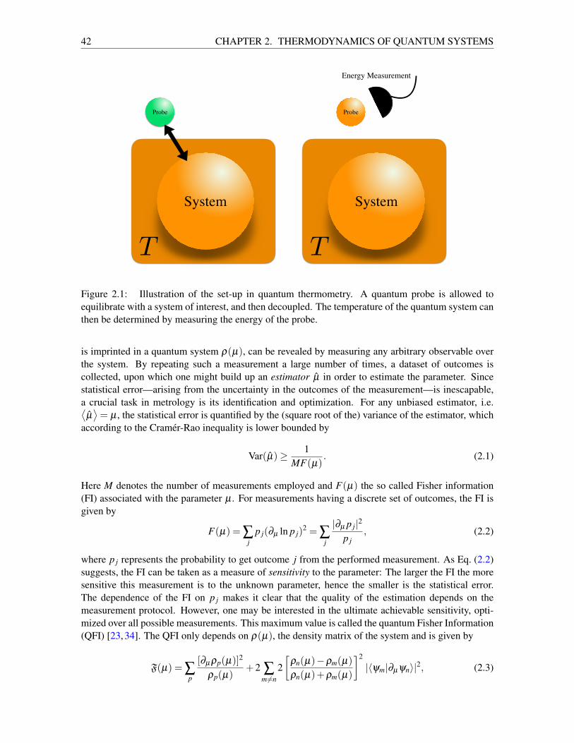
42 CHAPTER 2. THERMODYNAMICS OF QUANTUM SYSTEMS
T<latexit sha1_base64="+PBvf+lnnsnFY014vABWwPiSxYo=">AAAB6HicbVBNS8NAEJ3Ur1q/qh69LBbBU0lE0GPRi8cW+gVtKJvtpF272YTdjVBCf4EXD4p49Sd589+4bXPQ1gcDj/dmmJkXJIJr47rfTmFjc2t7p7hb2ts/ODwqH5+0dZwqhi0Wi1h1A6pRcIktw43AbqKQRoHATjC5n/udJ1Sax7Jppgn6ER1JHnJGjZUazUG54lbdBcg68XJSgRz1QfmrP4xZGqE0TFCte56bGD+jynAmcFbqpxoTyiZ0hD1LJY1Q+9ni0Bm5sMqQhLGyJQ1ZqL8nMhppPY0C2xlRM9ar3lz8z+ulJrz1My6T1KBky0VhKoiJyfxrMuQKmRFTSyhT3N5K2JgqyozNpmRD8FZfXiftq6rnVr3GdaV2l8dRhDM4h0vw4AZq8AB1aAEDhGd4hTfn0Xlx3p2PZWvByWdO4Q+czx+vqYzY</latexit><latexit sha1_base64="+PBvf+lnnsnFY014vABWwPiSxYo=">AAAB6HicbVBNS8NAEJ3Ur1q/qh69LBbBU0lE0GPRi8cW+gVtKJvtpF272YTdjVBCf4EXD4p49Sd589+4bXPQ1gcDj/dmmJkXJIJr47rfTmFjc2t7p7hb2ts/ODwqH5+0dZwqhi0Wi1h1A6pRcIktw43AbqKQRoHATjC5n/udJ1Sax7Jppgn6ER1JHnJGjZUazUG54lbdBcg68XJSgRz1QfmrP4xZGqE0TFCte56bGD+jynAmcFbqpxoTyiZ0hD1LJY1Q+9ni0Bm5sMqQhLGyJQ1ZqL8nMhppPY0C2xlRM9ar3lz8z+ulJrz1My6T1KBky0VhKoiJyfxrMuQKmRFTSyhT3N5K2JgqyozNpmRD8FZfXiftq6rnVr3GdaV2l8dRhDM4h0vw4AZq8AB1aAEDhGd4hTfn0Xlx3p2PZWvByWdO4Q+czx+vqYzY</latexit><latexit sha1_base64="+PBvf+lnnsnFY014vABWwPiSxYo=">AAAB6HicbVBNS8NAEJ3Ur1q/qh69LBbBU0lE0GPRi8cW+gVtKJvtpF272YTdjVBCf4EXD4p49Sd589+4bXPQ1gcDj/dmmJkXJIJr47rfTmFjc2t7p7hb2ts/ODwqH5+0dZwqhi0Wi1h1A6pRcIktw43AbqKQRoHATjC5n/udJ1Sax7Jppgn6ER1JHnJGjZUazUG54lbdBcg68XJSgRz1QfmrP4xZGqE0TFCte56bGD+jynAmcFbqpxoTyiZ0hD1LJY1Q+9ni0Bm5sMqQhLGyJQ1ZqL8nMhppPY0C2xlRM9ar3lz8z+ulJrz1My6T1KBky0VhKoiJyfxrMuQKmRFTSyhT3N5K2JgqyozNpmRD8FZfXiftq6rnVr3GdaV2l8dRhDM4h0vw4AZq8AB1aAEDhGd4hTfn0Xlx3p2PZWvByWdO4Q+czx+vqYzY</latexit><latexit sha1_base64="+PBvf+lnnsnFY014vABWwPiSxYo=">AAAB6HicbVBNS8NAEJ3Ur1q/qh69LBbBU0lE0GPRi8cW+gVtKJvtpF272YTdjVBCf4EXD4p49Sd589+4bXPQ1gcDj/dmmJkXJIJr47rfTmFjc2t7p7hb2ts/ODwqH5+0dZwqhi0Wi1h1A6pRcIktw43AbqKQRoHATjC5n/udJ1Sax7Jppgn6ER1JHnJGjZUazUG54lbdBcg68XJSgRz1QfmrP4xZGqE0TFCte56bGD+jynAmcFbqpxoTyiZ0hD1LJY1Q+9ni0Bm5sMqQhLGyJQ1ZqL8nMhppPY0C2xlRM9ar3lz8z+ulJrz1My6T1KBky0VhKoiJyfxrMuQKmRFTSyhT3N5K2JgqyozNpmRD8FZfXiftq6rnVr3GdaV2l8dRhDM4h0vw4AZq8AB1aAEDhGd4hTfn0Xlx3p2PZWvByWdO4Q+czx+vqYzY</latexit>
T<latexit sha1_base64="+PBvf+lnnsnFY014vABWwPiSxYo=">AAAB6HicbVBNS8NAEJ3Ur1q/qh69LBbBU0lE0GPRi8cW+gVtKJvtpF272YTdjVBCf4EXD4p49Sd589+4bXPQ1gcDj/dmmJkXJIJr47rfTmFjc2t7p7hb2ts/ODwqH5+0dZwqhi0Wi1h1A6pRcIktw43AbqKQRoHATjC5n/udJ1Sax7Jppgn6ER1JHnJGjZUazUG54lbdBcg68XJSgRz1QfmrP4xZGqE0TFCte56bGD+jynAmcFbqpxoTyiZ0hD1LJY1Q+9ni0Bm5sMqQhLGyJQ1ZqL8nMhppPY0C2xlRM9ar3lz8z+ulJrz1My6T1KBky0VhKoiJyfxrMuQKmRFTSyhT3N5K2JgqyozNpmRD8FZfXiftq6rnVr3GdaV2l8dRhDM4h0vw4AZq8AB1aAEDhGd4hTfn0Xlx3p2PZWvByWdO4Q+czx+vqYzY</latexit><latexit sha1_base64="+PBvf+lnnsnFY014vABWwPiSxYo=">AAAB6HicbVBNS8NAEJ3Ur1q/qh69LBbBU0lE0GPRi8cW+gVtKJvtpF272YTdjVBCf4EXD4p49Sd589+4bXPQ1gcDj/dmmJkXJIJr47rfTmFjc2t7p7hb2ts/ODwqH5+0dZwqhi0Wi1h1A6pRcIktw43AbqKQRoHATjC5n/udJ1Sax7Jppgn6ER1JHnJGjZUazUG54lbdBcg68XJSgRz1QfmrP4xZGqE0TFCte56bGD+jynAmcFbqpxoTyiZ0hD1LJY1Q+9ni0Bm5sMqQhLGyJQ1ZqL8nMhppPY0C2xlRM9ar3lz8z+ulJrz1My6T1KBky0VhKoiJyfxrMuQKmRFTSyhT3N5K2JgqyozNpmRD8FZfXiftq6rnVr3GdaV2l8dRhDM4h0vw4AZq8AB1aAEDhGd4hTfn0Xlx3p2PZWvByWdO4Q+czx+vqYzY</latexit><latexit sha1_base64="+PBvf+lnnsnFY014vABWwPiSxYo=">AAAB6HicbVBNS8NAEJ3Ur1q/qh69LBbBU0lE0GPRi8cW+gVtKJvtpF272YTdjVBCf4EXD4p49Sd589+4bXPQ1gcDj/dmmJkXJIJr47rfTmFjc2t7p7hb2ts/ODwqH5+0dZwqhi0Wi1h1A6pRcIktw43AbqKQRoHATjC5n/udJ1Sax7Jppgn6ER1JHnJGjZUazUG54lbdBcg68XJSgRz1QfmrP4xZGqE0TFCte56bGD+jynAmcFbqpxoTyiZ0hD1LJY1Q+9ni0Bm5sMqQhLGyJQ1ZqL8nMhppPY0C2xlRM9ar3lz8z+ulJrz1My6T1KBky0VhKoiJyfxrMuQKmRFTSyhT3N5K2JgqyozNpmRD8FZfXiftq6rnVr3GdaV2l8dRhDM4h0vw4AZq8AB1aAEDhGd4hTfn0Xlx3p2PZWvByWdO4Q+czx+vqYzY</latexit><latexit sha1_base64="+PBvf+lnnsnFY014vABWwPiSxYo=">AAAB6HicbVBNS8NAEJ3Ur1q/qh69LBbBU0lE0GPRi8cW+gVtKJvtpF272YTdjVBCf4EXD4p49Sd589+4bXPQ1gcDj/dmmJkXJIJr47rfTmFjc2t7p7hb2ts/ODwqH5+0dZwqhi0Wi1h1A6pRcIktw43AbqKQRoHATjC5n/udJ1Sax7Jppgn6ER1JHnJGjZUazUG54lbdBcg68XJSgRz1QfmrP4xZGqE0TFCte56bGD+jynAmcFbqpxoTyiZ0hD1LJY1Q+9ni0Bm5sMqQhLGyJQ1ZqL8nMhppPY0C2xlRM9ar3lz8z+ulJrz1My6T1KBky0VhKoiJyfxrMuQKmRFTSyhT3N5K2JgqyozNpmRD8FZfXiftq6rnVr3GdaV2l8dRhDM4h0vw4AZq8AB1aAEDhGd4hTfn0Xlx3p2PZWvByWdO4Q+czx+vqYzY</latexit>
Energy Measurement
System System
Probe Probe
Figure 2.1: Illustration of the set-up in quantum thermometry. A quantum probe is allowed toequilibrate with a system of interest, and then decoupled. The temperature of the quantum system canthen be determined by measuring the energy of the probe.
is imprinted in a quantum system ρ(µ), can be revealed by measuring any arbitrary observable overthe system. By repeating such a measurement a large number of times, a dataset of outcomes iscollected, upon which one might build up an estimator µ in order to estimate the parameter. Sincestatistical error—arising from the uncertainty in the outcomes of the measurement—is inescapable,a crucial task in metrology is its identification and optimization. For any unbiased estimator, i.e.⟨µ⟩= µ , the statistical error is quantified by the (square root of the) variance of the estimator, which
according to the Cramer-Rao inequality is lower bounded by
Var(µ)≥ 1MF(µ)
. (2.1)
Here M denotes the number of measurements employed and F(µ) the so called Fisher information(FI) associated with the parameter µ . For measurements having a discrete set of outcomes, the FI isgiven by
F(µ) = ∑j
p j(∂µ ln p j)2 = ∑
j
|∂µ p j|2p j
, (2.2)
where p j represents the probability to get outcome j from the performed measurement. As Eq. (2.2)suggests, the FI can be taken as a measure of sensitivity to the parameter: The larger the FI the moresensitive this measurement is to the unknown parameter, hence the smaller is the statistical error.The dependence of the FI on p j makes it clear that the quality of the estimation depends on themeasurement protocol. However, one may be interested in the ultimate achievable sensitivity, opti-mized over all possible measurements. This maximum value is called the quantum Fisher Information(QFI) [23, 34]. The QFI only depends on ρ(µ), the density matrix of the system and is given by
F(µ) = ∑p
[∂µρp(µ)]2
ρp(µ)+2 ∑
m6=n2[
ρn(µ)−ρm(µ)
ρn(µ)+ρm(µ)
]2
|〈ψm|∂µψn〉|2, (2.3)
2.1. QUANTUM THERMOMETRY 43
with ρp the eigenvalues of the density matrix of the system, and |ψi〉 are the eigenstates of the system.Replacing F(µ) with F(µ) in Eq. (2.1) gives us the quantum Cramer-Rao bound.
If we assume the system is already at thermal equilibrium, and therefore in a canonical Gibbsstate, ρeq = exp(−βH)/Z, the QFI associated to temperature can be simplified by noticing that theeigenstates entering the second term of the RHS of Eq. (2.3) do not change with temperature, andtherefore this term is identically zero. Thus for a thermal state, F(µ) is fully determined by thechange of the density matrix eigenvalues with temperature. Hence, for a d-dimensional Gibbs stateρeq, F(µ) can be easily evaluated and is equal to the classical Fisher information corresponding to ameasurement described by the eigenstates of the Hamiltonian H. In formula one obtains [10, 12, 35,53]
F(β ) =d
∑n=1
|∂T pn|2pn
= β4 [Var(H)]2 , (2.4)
where as before β = 1/kBT .
2.1.1 Thermometry for Harmonic Spectra
Let us consider using a harmonically spaced quantum system, with energy gap ∆, as a thermometer.For a thermal two level system with free Hamiltonian H = ∆/2σz, the corresponding Gibbs state is
ρeq =
12
(1− tanh(β∆/2) 0
0 1+ tanh(β∆/2)
). (2.5)
We can determine the QFI using Eq. (2.4) and find
F(β ) =β 4∆2
2sech2 (β∆/2) . (2.6)
It is also straight forward to consider the infinite-dimensional quantum harmonic oscillator, H =∆(a†a+ 1/2) (a representing the bosonic annihilation operator satisfying [a,a†] = I), with the samespectral gap ∆. The QFI for a thermal state is given by
F(β ) =β 4∆2
4csch2 (β∆/2) . (2.7)
In Fig. 2.2 (a) the solid (dashed) curves show the QFI for several values of the energy levelsplitting, ∆, for the two-level system (harmonic oscillator). Clearly, smaller energy gaps can lead tosignificantly better precision, however an important point to note is that the QFI peaks at a singlevalue of T . This means there is a single temperature that a given system with a specified energy gapis optimized to probe. This temperature corresponds to the value of T maximizing the QFI, Fmax, andas we change ∆ the position of this peak shifts. An intuitive understanding of this can be drawn bycloser consideration of Eq. (2.4): for sufficiently low temperatures, regardless of dimensionality, thequantum thermometer will be in its ground state. Since the sensitivity is related to how the thermalpopulations change, smaller gaps between the eigenstates result in rapid rates of change for lowtemperatures since more energy levels become populated at these temperatures. Conversely, whenthe spectral gap is larger, the system requires larger temperatures before any of the excited statesbecome populated.
From Fig. 2.2 we clearly see that the two disparate dimensional systems exhibit qualitatively iden-tical behaviors, thus implying that the achievable precision for thermometry with harmonic systems issolely dependent on the single characteristic spectral gap, ∆, while dimensionality plays only a minorrole. We can show this more explicitly by considering arbitrary d-dimensional harmonic systems,
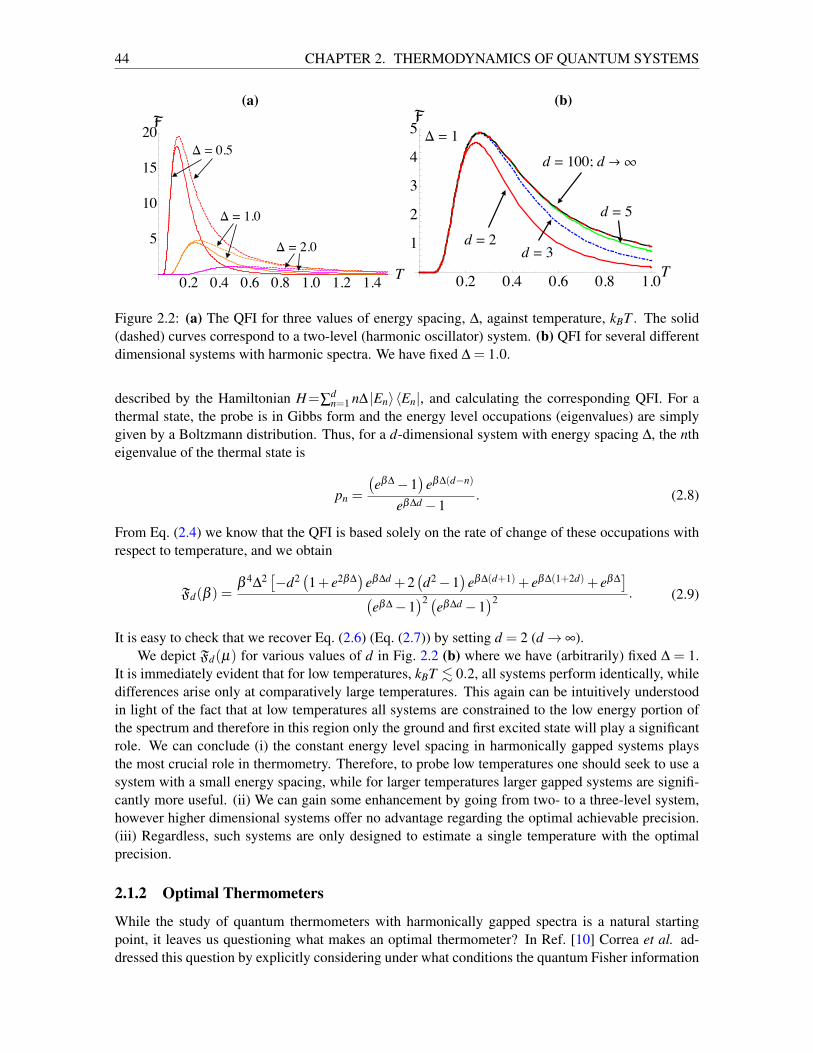
44 CHAPTER 2. THERMODYNAMICS OF QUANTUM SYSTEMS
(a) (b)
! " 0.5
! " 1.0
! " 2.0
0.2 0.4 0.6 0.8 1.0 1.2 1.4 T
5
10
15
20!
d ! 100; d "#
d ! 5
d ! 2d ! 3
$ ! 1
0.2 0.4 0.6 0.8 1.0T
1
2
3
4
5!
Figure 2.2: (a) The QFI for three values of energy spacing, ∆, against temperature, kBT . The solid(dashed) curves correspond to a two-level (harmonic oscillator) system. (b) QFI for several differentdimensional systems with harmonic spectra. We have fixed ∆ = 1.0.
described by the Hamiltonian H=∑dn=1 n∆ |En〉〈En|, and calculating the corresponding QFI. For a
thermal state, the probe is in Gibbs form and the energy level occupations (eigenvalues) are simplygiven by a Boltzmann distribution. Thus, for a d-dimensional system with energy spacing ∆, the ntheigenvalue of the thermal state is
pn =
(eβ∆−1
)eβ∆(d−n)
eβ∆d−1. (2.8)
From Eq. (2.4) we know that the QFI is based solely on the rate of change of these occupations withrespect to temperature, and we obtain
Fd(β ) =β 4∆2
[−d2
(1+ e2β∆
)eβ∆d +2
(d2−1
)eβ∆(d+1)+ eβ∆(1+2d)+ eβ∆
](eβ∆−1
)2 (eβ∆d−1)2 . (2.9)
It is easy to check that we recover Eq. (2.6) (Eq. (2.7)) by setting d = 2 (d→ ∞).We depict Fd(µ) for various values of d in Fig. 2.2 (b) where we have (arbitrarily) fixed ∆ = 1.
It is immediately evident that for low temperatures, kBT . 0.2, all systems perform identically, whiledifferences arise only at comparatively large temperatures. This again can be intuitively understoodin light of the fact that at low temperatures all systems are constrained to the low energy portion ofthe spectrum and therefore in this region only the ground and first excited state will play a significantrole. We can conclude (i) the constant energy level spacing in harmonically gapped systems playsthe most crucial role in thermometry. Therefore, to probe low temperatures one should seek to use asystem with a small energy spacing, while for larger temperatures larger gapped systems are signifi-cantly more useful. (ii) We can gain some enhancement by going from two- to a three-level system,however higher dimensional systems offer no advantage regarding the optimal achievable precision.(iii) Regardless, such systems are only designed to estimate a single temperature with the optimalprecision.
2.1.2 Optimal Thermometers
While the study of quantum thermometers with harmonically gapped spectra is a natural startingpoint, it leaves us questioning what makes an optimal thermometer? In Ref. [10] Correa et al. ad-dressed this question by explicitly considering under what conditions the quantum Fisher information
2.2. QUANTUM HEAT ENGINES – ENGINES WITH ATOMIC WORKING FLUIDS 45
in Eq. (2.4) is maximized. It is immediately evident that a probe with the maximum possible energyvariance at equilibrium fulfills the task. Considering an arbitrary N-dimensional system, this is equiv-alent to insisting that the heat capacity of the probe is maximal. Such an optimal thermometer is aneffective two-level system, with a unique ground state and an (N− 1)-fold degenerate excited state.The corresponding precision scales with the dimensionality of the probe, however this comes at a costof having a reduced specified temperature range for which it operates efficiently [10]. Clearly theseoptimal thermometers again have a single characteristic energy splitting and therefore are designed toestimate a single temperature precisely. However, just as exploiting degeneracy is shown to enhanceprecision, including anharmonicity can also increase the range of temperatures that can be preciselyprobed [9].1
2.2 Quantum heat engines – engines with atomic working fluids
Now that we have understood the limitations in measuring temperature in quantum systems, we cancontinue to apply the conceptual framework to the most important application of quantum thermody-namics – quantum heat engines. We have already seen an example of a quantum thermodynamic cyclein Sec. 1.4 – the Carnot cycle. In the following, we will instead focus on arguably the most widelyused cyclic process: the Otto cycle [1,15,26,38,39,43]. The Otto cycle underlies the working princi-ples of all internal combustion heat engines and is therefore of significant practical and fundamentalrelevance [see Fig. 2.3 for a real example].
In what follows we will begin outlining the basic strokes involved in the classical formulation ofthe Otto cycle before looking into its quantum mechanical description. Some time will be dedicatedto highlighting the subtle differences between the Carnot and Otto cycles and we will explore twoparadigmatic instances of the quantum Otto cycle where the working substance is a two-level systemand a quantum harmonic oscillator, the latter which was recently used to realize the first experimentaldemonstration of a genuinely quantum heat engine.
2.2.1 The Otto Cycle: Classical to quantum formulation
The Otto cycle, named after the German engineer Nikolaus Otto who is accredited with building thefirst working four-stroke engine based on the design by Alphonse Beau de Rochas, consists of thefollowing thermodynamic processes between local equilibrium states A,B,C,D:
1. Adiabatic (isentropic) compression (A→ B): The working medium is compressed. This strokeinvolves both volume and temperature changes, while the entropy remains constant.
2. Isochoric heating (B→C): The volume of the working medium is fixed, while the temperatureis increased.
3. Adiabatic (isentropic) expansion (C→ D): The power stroke, when useful work is extractedfrom the engine. Again this stroke involves both volume and temperature changes, at fixedentropy.
4. Isochoric cooling (D→ A): The working medium is cooled at a fixed volume and returned toits initial state, ready to begin the cycle again.
In order to clearly define the quantum Otto cycle it is important to determine how these four strokesare realized when the working medium is a quantum system. To this end, it is important to examineadiabatic and isochoric processes for quantum systems [38, 39].
1For a more expansive review of thermometry we refer to Ref. [30].
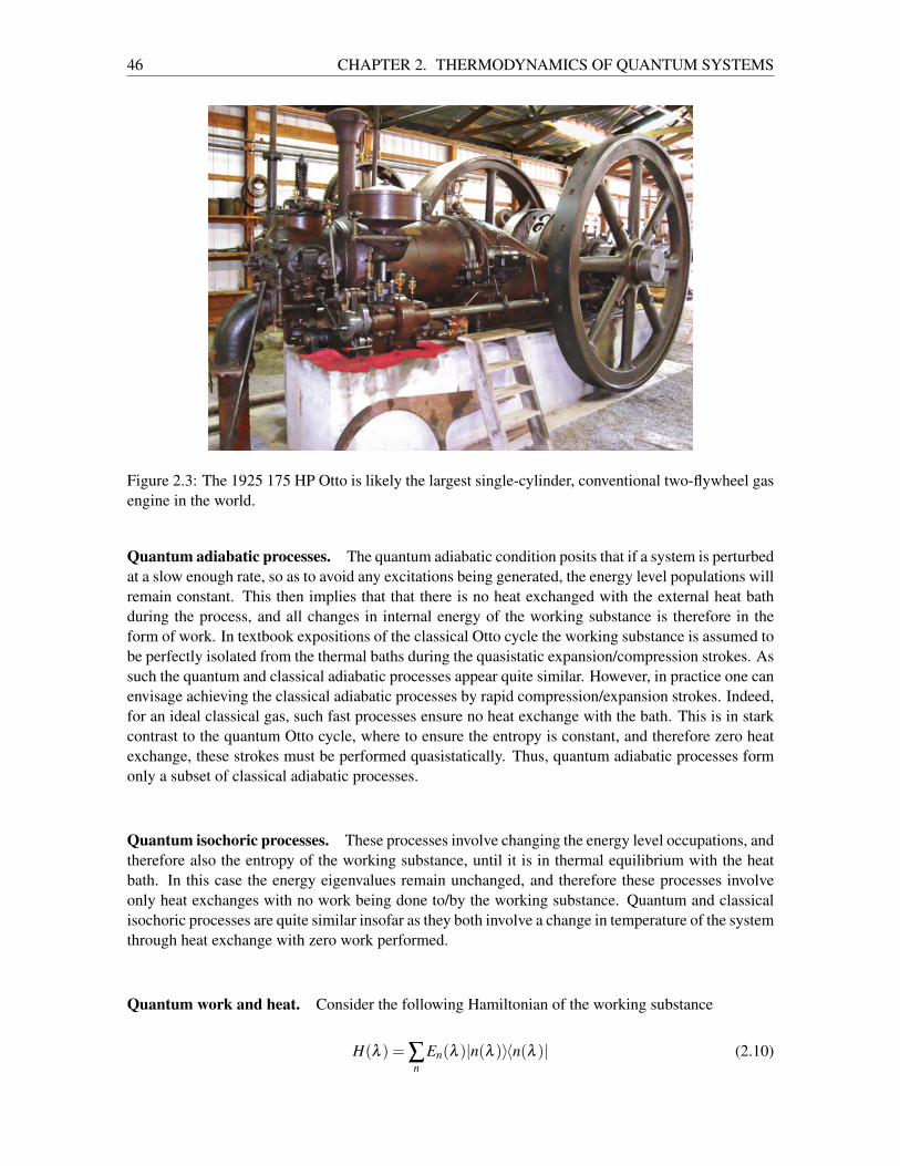
46 CHAPTER 2. THERMODYNAMICS OF QUANTUM SYSTEMS
Figure 2.3: The 1925 175 HP Otto is likely the largest single-cylinder, conventional two-flywheel gasengine in the world.
Quantum adiabatic processes. The quantum adiabatic condition posits that if a system is perturbedat a slow enough rate, so as to avoid any excitations being generated, the energy level populations willremain constant. This then implies that that there is no heat exchanged with the external heat bathduring the process, and all changes in internal energy of the working substance is therefore in theform of work. In textbook expositions of the classical Otto cycle the working substance is assumed tobe perfectly isolated from the thermal baths during the quasistatic expansion/compression strokes. Assuch the quantum and classical adiabatic processes appear quite similar. However, in practice one canenvisage achieving the classical adiabatic processes by rapid compression/expansion strokes. Indeed,for an ideal classical gas, such fast processes ensure no heat exchange with the bath. This is in starkcontrast to the quantum Otto cycle, where to ensure the entropy is constant, and therefore zero heatexchange, these strokes must be performed quasistatically. Thus, quantum adiabatic processes formonly a subset of classical adiabatic processes.
Quantum isochoric processes. These processes involve changing the energy level occupations, andtherefore also the entropy of the working substance, until it is in thermal equilibrium with the heatbath. In this case the energy eigenvalues remain unchanged, and therefore these processes involveonly heat exchanges with no work being done to/by the working substance. Quantum and classicalisochoric processes are quite similar insofar as they both involve a change in temperature of the systemthrough heat exchange with zero work performed.
Quantum work and heat. Consider the following Hamiltonian of the working substance
H(λ ) = ∑n
En(λ )|n(λ )〉〈n(λ )| (2.10)
2.2. QUANTUM HEAT ENGINES – ENGINES WITH ATOMIC WORKING FLUIDS 47
with |n(λ )〉 the energy eigenstates, En the associated energy eigenvalues, and λ a variable workparameter. It is convenient to rescale the energy with respect to the ground state energy
H(λ ) = ∑n(En−E0)(λ )|n(λ )〉〈n(λ )|. (2.11)
The internal energy is then simply given by the expectation value of this Hamiltonian over the stateof the working substance
E = 〈H〉= ∑n
pnEn (2.12)
where as before, pn = exp(−βEn)/Z. From the first law (see Sec. 1.1), we can then split the changein internal energy into a work and heat contribution
dE = ∑n(pndEn +End pn) = dW + dQ. (2.13)
From Eq. (2.13) it is easy to identify when a process is quantum adiabatic and/or isochoric. In anadiabatic process, the eigenenergies vary while their populations, and therefore the entropy of theworking substance, are kept constant. Thus, d pn = 0 and the change in internal energy is attributedsolely to work. Conversely, isochoric processes change the populations without affecting the energyeigenvalues, hence dEn = 0 and as such the change in internal energy is due purely to heat exchanges.At this point it is useful to highlight one significant difference between idealized Carnot and Ottocycles. While both involve two adiabatic transformations, in a Carnot cycle heat is absorbed/emittedthrough isothermal processes. The system must remain in thermal equilibrium, at temperature T ofthe bath, while the heating/cooling process occurs. Therefore, an ideal isothermal process will requirechanges in both En and pn, implying work done and heat exchange. Under the strict condition that thetemperature of the working substance is equal to that of the heat bath at the end of the adiabatic strokein the Carnot cycle, the ensuing isothermal process is thermodynamically reversible, i.e. results inzero irreversible entropy production. The Otto cycle, on the other hand, only requires the workingsubstance to be in local thermal equilibrium at the end of each stroke. Therefore, at the end of theadiabatic power stroke C → D the working substance will be in a thermal state with temperaturegiven by the hot heat bath, Th. It is then connected to the cool heat bath in order to thermalize tothe initial state through the isochoric cooling. This cooling is accompanied by an irreversible entropyproduction. Therefore, it is important to keep in mind that while the expressions for the maximalefficiency of the ideal Carnot and Otto cycles share several similar features, the underlying physicalprocesses are fundamentally different.
2.2.2 A two-level Otto cycle
To solidify the ideas let us consider an Otto cycle when the working substance is a two-level system(TLS) with energy eigenvalues Eg, Ee and corresponding eigenstates |ψg〉 , |ψe〉 [38]. Notethat we have dropped the explicit dependence on the work parameter λ for brevity, since in whatfollows we will only be concerned with the state of the TLS at the beginning and end of each stroke.Following from Eq. (2.11) we can rescale the Hamiltonian such that Eg = 0 and therefore
H = (Ee−Eg) |ψe〉〈ψe|= ∆ |ψe〉〈ψe| (2.14)
where ∆ is the energy difference between ground and excited states. The corresponding thermal stateat temperature T is given by Eq. (2.5), which we can also write as
ρeq ≡ pg|ψg〉〈ψg|+ pe|ψe〉〈ψe|. (2.15)
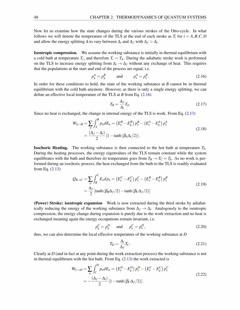
48 CHAPTER 2. THERMODYNAMICS OF QUANTUM SYSTEMS
Now let us examine how the state changes during the various strokes of the Otto-cycle. In whatfollows we will denote the temperature of the TLS at the end of each stroke as Ti for i = A,B,C,Dand allow the energy splitting ∆ to vary between ∆i and ∆ f with ∆ f > ∆i.
Isentropic compression. We assume the working substance is initially in thermal equilibrium witha cold bath at temperature Tc, and therefore Tc = TA. During the adiabatic stroke work is performedon the TLS to increase energy splitting from ∆i → ∆ f without any exchange of heat. This requiresthat the populations at the start and end of the process are equal, i.e.
pAg = pB
g and pAe = pB
e . (2.16)
In order for these conditions to hold, the state of the working substance at B cannot be in thermalequilibrium with the cold bath anymore. However, as there is only a single energy splitting, we candefine an effective local temperature of the TLS at B from Eq. (2.16)
TB =∆ f
∆iTA. (2.17)
Since no heat is exchanged, the change in internal energy of the TLS is work. From Eq. (2.13)
WA→B = ∑n
∫ B
ApndEn =
(EB
e −EBg)
pBe −(EA
e −EAg)
pAe
=(∆ f −∆i)
2[1− tanh(βA∆i/2)] .
(2.18)
Isochoric Heating. The working substance is then connected to the hot bath at temperature Th.During the heating processes, the energy eigenvalues of the TLS remain constant while the systemequilibrates with the bath and therefore its temperature goes from TB→ TC = Th. As no work is per-formed during an isochoric process, the heat exchanged from the bath to the TLS is readily evaluatedfrom Eq. (2.13)
QB→C = ∑n
∫ C
BEnd pn =
(EC
e −ECg)
pCe −(EB
e −EBg)
pBe
=∆ f
2[tanh(βB∆ f /2)− tanh(βC∆ f /2)]
(2.19)
(Power) Stroke: isentropic expansion Work is now extracted during the third stroke by adiabat-ically reducing the energy of the working substance from ∆ f → ∆i. Analogously to the isentropiccompression, the energy change during expansion is purely due to the work extraction and no heat isexchanged meaning again the energy occupations remain invariant, i.e.
pCg = pD
g and pCe = pD
e , (2.20)
thus, we can also determine the local effective temperature of the working substance at D
TD =∆i
∆ fTC. (2.21)
Clearly at D (and in fact at any point during the work extraction process) the working substance is notin thermal equilibrium with the hot bath. From Eq. (2.13) the work extracted is
WC→D = ∑n
∫ D
CpndEn =
(ED
e −EDg)
pDe −
(EC
e −ECg)
pCe
=−(∆ f −∆i)
2[1− tanh(βC∆ f /2)] .
(2.22)
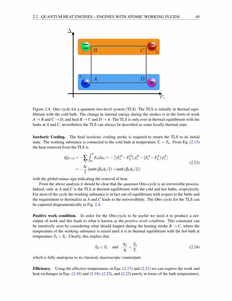
2.2. QUANTUM HEAT ENGINES – ENGINES WITH ATOMIC WORKING FLUIDS 49
A
B C
D
Th
Tc
Pe
Figure 2.4: Otto cycle for a quantum two-level system (TLS). The TLS is initially in thermal equi-librium with the cold bath. The change in internal energy during the strokes is in the form of workA→ B and C→D, and heat B→C and D→ A. The TLS is only ever in thermal equilibrium with thebaths at A and C, nevertheless the TLS can always be described as some locally thermal state.
Isochoric Cooling. The final isochoric cooling stroke is required to return the TLS to its initialstate. The working substance is connected to the cold bath at temperature Tc = TA. From Eq. (2.13)the heat removed from the TLS is
QD→A =−∑n
∫ A
DEnd pn =−
[(ED
e −EDg)
pDe −
(EA
e −EAg)
pAe]
=−∆i
2[tanh(βD∆i/2)+ tanh(βA∆i/2)]
(2.23)
with the global minus sign indicating the removal of heat.From the above analysis it should be clear that the quantum Otto-cycle is an irreversible process.
Indeed, only at A and C is the TLS at thermal equilibrium with the cold and hot baths, respectively.For most of the cycle the working substance is in fact out-of-equilibrium with respect to the baths andthe requirement to thermalize at A and C leads to the irreversibility. The Otto cycle for the TLS canbe captured diagrammatically in Fig. 2.4.
Positive work condition. In order for the Otto-cycle to be useful we need it to produce a net-output of work and this leads to what is known as the positive work condition. This constraint canbe intuitively seen by considering what should happen during the heating stroke B→ C, where thetemperature of the working substance is raised until it is in thermal equilibrium with the hot bath attemperature Th = TC. Clearly, this implies that
TB < TC and∆ f
∆i<
Th
Tc(2.24)
which is fully analogous to its classical, macroscopic counterpart.
Efficiency. Using the effective temperatures in Eqs. (2.17) and (2.21) we can express the work andheat exchanges in Eqs. (2.18) and (2.19), (2.22), and (2.23) purely in terms of the bath temperatures,
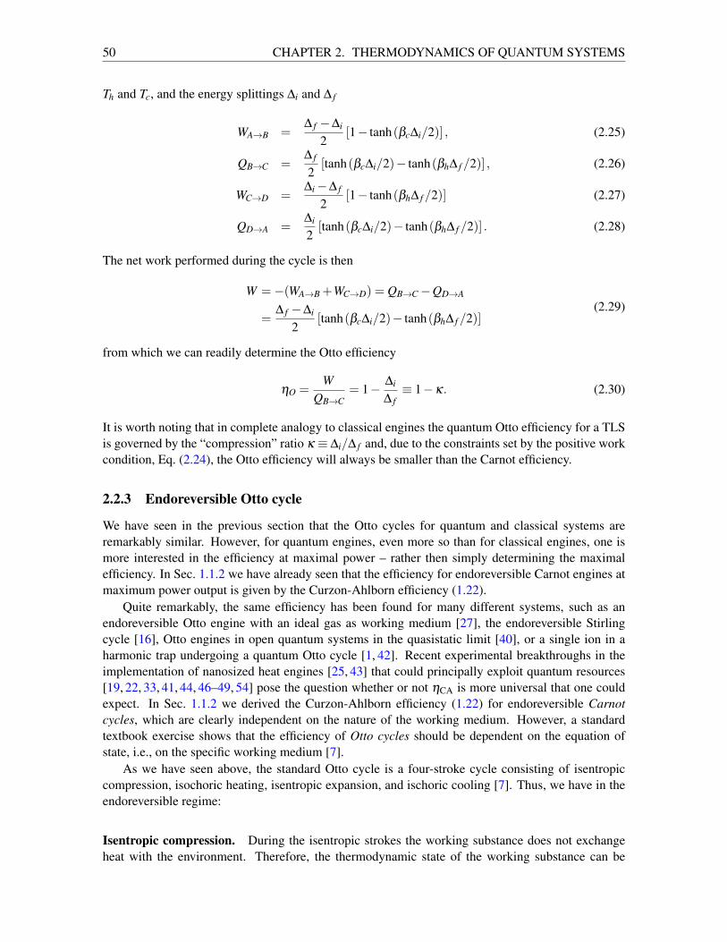
50 CHAPTER 2. THERMODYNAMICS OF QUANTUM SYSTEMS
Th and Tc, and the energy splittings ∆i and ∆ f
WA→B =∆ f −∆i
2[1− tanh(βc∆i/2)] , (2.25)
QB→C =∆ f
2[tanh(βc∆i/2)− tanh(βh∆ f /2)] , (2.26)
WC→D =∆i−∆ f
2[1− tanh(βh∆ f /2)] (2.27)
QD→A =∆i
2[tanh(βc∆i/2)− tanh(βh∆ f /2)] . (2.28)
The net work performed during the cycle is then
W =−(WA→B +WC→D) = QB→C−QD→A
=∆ f −∆i
2[tanh(βc∆i/2)− tanh(βh∆ f /2)]
(2.29)
from which we can readily determine the Otto efficiency
ηO =W
QB→C= 1− ∆i
∆ f≡ 1−κ. (2.30)
It is worth noting that in complete analogy to classical engines the quantum Otto efficiency for a TLSis governed by the “compression” ratio κ ≡ ∆i/∆ f and, due to the constraints set by the positive workcondition, Eq. (2.24), the Otto efficiency will always be smaller than the Carnot efficiency.
2.2.3 Endoreversible Otto cycle
We have seen in the previous section that the Otto cycles for quantum and classical systems areremarkably similar. However, for quantum engines, even more so than for classical engines, one ismore interested in the efficiency at maximal power – rather then simply determining the maximalefficiency. In Sec. 1.1.2 we have already seen that the efficiency for endoreversible Carnot engines atmaximum power output is given by the Curzon-Ahlborn efficiency (1.22).
Quite remarkably, the same efficiency has been found for many different systems, such as anendoreversible Otto engine with an ideal gas as working medium [27], the endoreversible Stirlingcycle [16], Otto engines in open quantum systems in the quasistatic limit [40], or a single ion in aharmonic trap undergoing a quantum Otto cycle [1, 42]. Recent experimental breakthroughs in theimplementation of nanosized heat engines [25, 43] that could principally exploit quantum resources[19, 22, 33, 41, 44, 46–49, 54] pose the question whether or not ηCA is more universal that one couldexpect. In Sec. 1.1.2 we derived the Curzon-Ahlborn efficiency (1.22) for endoreversible Carnotcycles, which are clearly independent on the nature of the working medium. However, a standardtextbook exercise shows that the efficiency of Otto cycles should be dependent on the equation ofstate, i.e., on the specific working medium [7].
As we have seen above, the standard Otto cycle is a four-stroke cycle consisting of isentropiccompression, isochoric heating, isentropic expansion, and ischoric cooling [7]. Thus, we have in theendoreversible regime:
Isentropic compression. During the isentropic strokes the working substance does not exchangeheat with the environment. Therefore, the thermodynamic state of the working substance can be
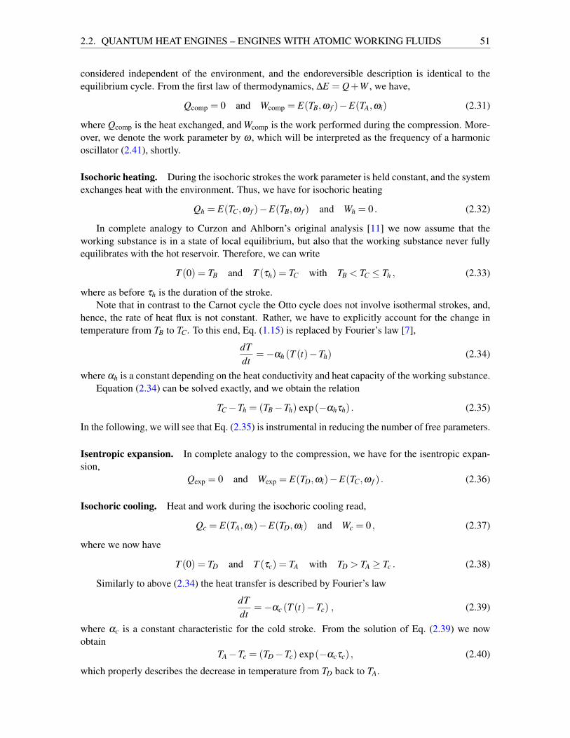
2.2. QUANTUM HEAT ENGINES – ENGINES WITH ATOMIC WORKING FLUIDS 51
considered independent of the environment, and the endoreversible description is identical to theequilibrium cycle. From the first law of thermodynamics, ∆E = Q+W , we have,
Qcomp = 0 and Wcomp = E(TB,ω f )−E(TA,ωi) (2.31)
where Qcomp is the heat exchanged, and Wcomp is the work performed during the compression. More-over, we denote the work parameter by ω , which will be interpreted as the frequency of a harmonicoscillator (2.41), shortly.
Isochoric heating. During the isochoric strokes the work parameter is held constant, and the systemexchanges heat with the environment. Thus, we have for isochoric heating
Qh = E(TC,ω f )−E(TB,ω f ) and Wh = 0 . (2.32)
In complete analogy to Curzon and Ahlborn’s original analysis [11] we now assume that theworking substance is in a state of local equilibrium, but also that the working substance never fullyequilibrates with the hot reservoir. Therefore, we can write
T (0) = TB and T (τh) = TC with TB < TC ≤ Th , (2.33)
where as before τh is the duration of the stroke.Note that in contrast to the Carnot cycle the Otto cycle does not involve isothermal strokes, and,
hence, the rate of heat flux is not constant. Rather, we have to explicitly account for the change intemperature from TB to TC. To this end, Eq. (1.15) is replaced by Fourier’s law [7],
dTdt
=−αh (T (t)−Th) (2.34)
where αh is a constant depending on the heat conductivity and heat capacity of the working substance.Equation (2.34) can be solved exactly, and we obtain the relation
TC−Th = (TB−Th) exp(−αhτh) . (2.35)
In the following, we will see that Eq. (2.35) is instrumental in reducing the number of free parameters.
Isentropic expansion. In complete analogy to the compression, we have for the isentropic expan-sion,
Qexp = 0 and Wexp = E(TD,ωi)−E(TC,ω f ) . (2.36)
Isochoric cooling. Heat and work during the isochoric cooling read,
Qc = E(TA,ωi)−E(TD,ωi) and Wc = 0 , (2.37)
where we now have
T (0) = TD and T (τc) = TA with TD > TA ≥ Tc . (2.38)
Similarly to above (2.34) the heat transfer is described by Fourier’s law
dTdt
=−αc (T (t)−Tc) , (2.39)
where αc is a constant characteristic for the cold stroke. From the solution of Eq. (2.39) we nowobtain
TA−Tc = (TD−Tc) exp(−αcτc) , (2.40)
which properly describes the decrease in temperature from TD back to TA.
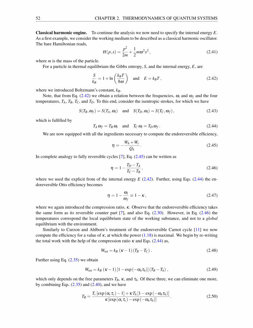
52 CHAPTER 2. THERMODYNAMICS OF QUANTUM SYSTEMS
Classical harmonic engine. To continue the analysis we now need to specify the internal energy E.As a first example, we consider the working medium to be described as a classical harmonic oscillator.The bare Hamiltonian reads,
H(p,x) =p2
2m+
12
mω2x2 , (2.41)
where m is the mass of the particle.For a particle in thermal equilibrium the Gibbs entropy, S, and the internal energy, E, are
SkB
= 1+ ln(
kBThω
)and E = kBT , (2.42)
where we introduced Boltzmann’s constant, kB.Note, that from Eq. (2.42) we obtain a relation between the frequencies, ωi and ω f and the four
temperatures, TA, TB, TC, and TD. To this end, consider the isentropic strokes, for which we have
S(TB,ω f ) = S(TA,ωi) and S(TD,ωi) = S(TC,ω f ) , (2.43)
which is fulfilled byTA ω f = TB ωi and TC ωi = TD ω f . (2.44)
We are now equipped with all the ingredients necessary to compute the endoreversible efficiency,
η =−Wh +Wc
Qh. (2.45)
In complete analogy to fully reversible cycles [7], Eq. (2.45) can be written as
η = 1− TD−TA
TC−TB, (2.46)
where we used the explicit from of the internal energy E (2.42). Further, using Eqs. (2.44) the en-doreversible Otto efficiency becomes
η = 1− ωi
ω f≡ 1−κ , (2.47)
where we again introduced the compression ratio, κ . Observe that the endoreversible efficiency takesthe same form as its reversible counter part [7], and also Eq. (2.30). However, in Eq. (2.46) thetemperatures correspond the local equilibrium state of the working substance, and not to a globalequilibrium with the environment.
Similarly to Curzon and Ahlborn’s treatment of the endoreversible Carnot cycle [11] we nowcompute the efficiency for a value of κ , at which the power (1.18) is maximal. We begin by re-writingthe total work with the help of the compression ratio κ and Eqs. (2.44) as,
Wtot = kB (κ−1)(TB−TC) . (2.48)
Further using Eq. (2.35) we obtain
Wtot = kB (κ−1) [1− exp(−αhτh)] (TB−Th) , (2.49)
which only depends on the free parameters TB, κ , and τh. Of these three, we can eliminate one more,by combining Eqs. (2.35) and (2.40), and we have
TB =Tc [exp(αcτc)−1]+κ Th [1− exp(−αhτh)]
κ [exp(αcτc)− exp(−αhτh)]. (2.50)
2.2. QUANTUM HEAT ENGINES – ENGINES WITH ATOMIC WORKING FLUIDS 53
Finally, the power output (1.18) takes the form,
P =2kB (κ−1)(Tc−κ Th)
ζ κ(τc + τh)
sinh(αcτc/2)sinh(αhτh/2)sinh [(αcτc +αhτh)/2]
. (2.51)
Remarkably the power output factorizes into a contribution that only depends on the compressionratio, κ , and another term that is governed by the stroke times, τc and τh,
P(κ,τh,τc) = f1(κ) f2(τh,τc) . (2.52)
It is then a simple exercise to show that P(κ,τh,τc) is maximized for any value of τh and τc if wehave,
Pmax = P(κmax) with κmax =
√Tc
Th. (2.53)
Therefore, the efficiency at maximal power reads,
η = 1−√
Tc
Th. (2.54)
In conclusion, we have shown analytically that for the classical harmonic oscillator the efficiencyat maximal power of an endoreversible Otto cycle (2.45) is indeed given by the Curzon-Ahlbornefficiency (1.22).
It is worth emphasizing that for the endoreversible Otto cycle we started with six free parameters,the four temperatures TA, TB, TC, and TD, and the two stroke times, τh and τc. Of these, we succeededin eliminating three, by explicitly using Fourier’s law for the heat transfer, Eqs. (2.34) and (2.39),and the explicit expressions for the entropy and the internal energy (2.42). Therefore, one would notexpect to obtain the same result (2.54) for other working substances such as the quantum harmonicoscillator.
Quantum Brownian engine. Next, we will analyze a quantum harmonic engine in the ultra-weakcoupling limit [51]. This situation is similar to the model studied in Ref. [40], however in the presentcase we will not have to solve the full quantum dynamics.
Accordingly, the internal energy reads
E =hω
2coth
(hω
2kBT
)(2.55)
and the entropy becomes
SkB
=hω
2kBTcoth
(hω
2kBT
)− ln
[12
sinh(
hω
2kBT
)]. (2.56)
Despite the functional form of S being more involved, we notice that the four temperatures and thetwo frequencies are still related by the same Eq. (2.44). Thus, it can be shown [40] that the efficiencyof an endoreversible Otto cycle in a quantum harmonic oscillators also reads,
η = 1−κ . (2.57)
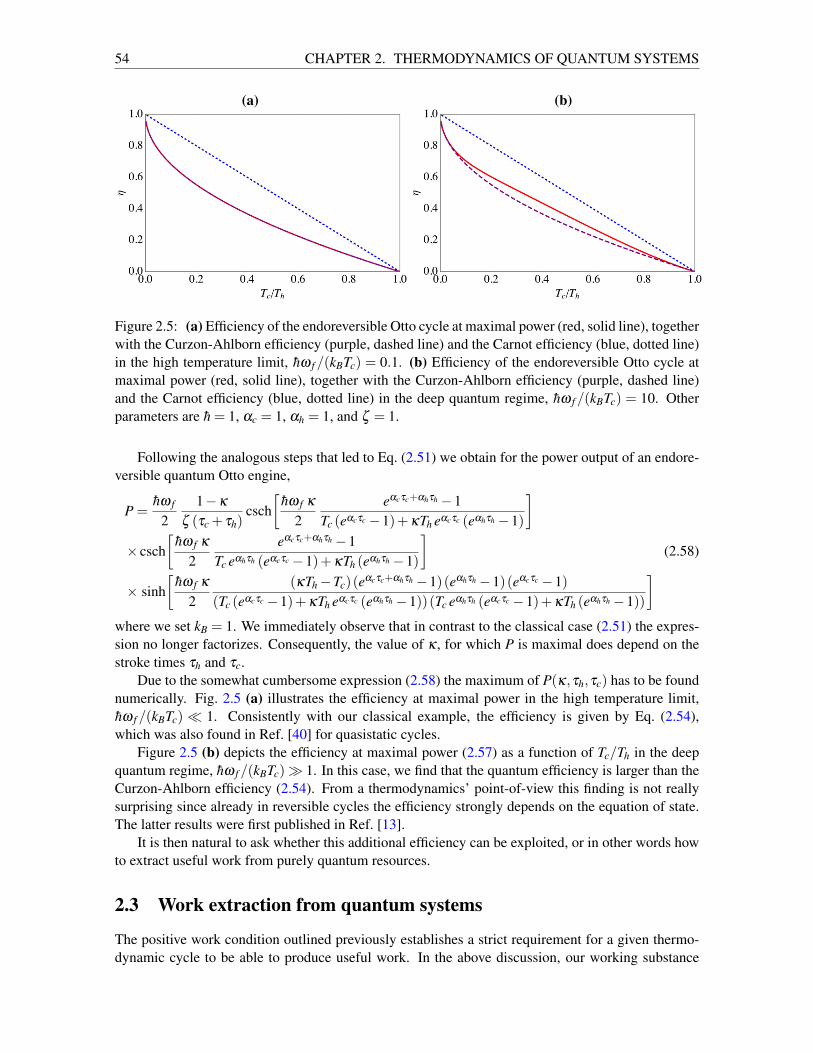
54 CHAPTER 2. THERMODYNAMICS OF QUANTUM SYSTEMS
(a) (b)
Figure 2.5: (a) Efficiency of the endoreversible Otto cycle at maximal power (red, solid line), togetherwith the Curzon-Ahlborn efficiency (purple, dashed line) and the Carnot efficiency (blue, dotted line)in the high temperature limit, hω f /(kBTc) = 0.1. (b) Efficiency of the endoreversible Otto cycle atmaximal power (red, solid line), together with the Curzon-Ahlborn efficiency (purple, dashed line)and the Carnot efficiency (blue, dotted line) in the deep quantum regime, hω f /(kBTc) = 10. Otherparameters are h = 1, αc = 1, αh = 1, and ζ = 1.
Following the analogous steps that led to Eq. (2.51) we obtain for the power output of an endore-versible quantum Otto engine,
P =hω f
21−κ
ζ (τc + τh)csch
[hω f κ
2eαcτc+αhτh−1
Tc (eαcτc−1)+κTh eαcτc (eαhτh−1)
]× csch
[hω f κ
2eαcτc+αhτh−1
Tc eαhτh (eαcτc−1)+κTh (eαhτh−1)
]× sinh
[hω f κ
2(κTh−Tc)(eαcτc+αhτh−1)(eαhτh−1)(eαcτc−1)
(Tc (eαcτc−1)+κTh eαcτc (eαhτh−1))(Tc eαhτh (eαcτc−1)+κTh (eαhτh−1))
] (2.58)
where we set kB = 1. We immediately observe that in contrast to the classical case (2.51) the expres-sion no longer factorizes. Consequently, the value of κ , for which P is maximal does depend on thestroke times τh and τc.
Due to the somewhat cumbersome expression (2.58) the maximum of P(κ,τh,τc) has to be foundnumerically. Fig. 2.5 (a) illustrates the efficiency at maximal power in the high temperature limit,hω f /(kBTc) 1. Consistently with our classical example, the efficiency is given by Eq. (2.54),which was also found in Ref. [40] for quasistatic cycles.
Figure 2.5 (b) depicts the efficiency at maximal power (2.57) as a function of Tc/Th in the deepquantum regime, hω f /(kBTc) 1. In this case, we find that the quantum efficiency is larger than theCurzon-Ahlborn efficiency (2.54). From a thermodynamics’ point-of-view this finding is not reallysurprising since already in reversible cycles the efficiency strongly depends on the equation of state.The latter results were first published in Ref. [13].
It is then natural to ask whether this additional efficiency can be exploited, or in other words howto extract useful work from purely quantum resources.
2.3 Work extraction from quantum systems
The positive work condition outlined previously establishes a strict requirement for a given thermo-dynamic cycle to be able to produce useful work. In the above discussion, our working substance
2.3. WORK EXTRACTION FROM QUANTUM SYSTEMS 55
Marlan Scully:The deep physics behind the second law of thermo-dynamics is not violated; nevertheless, the quantumCarnot engine has certain features that are not possi-ble in a classical engine [49].
was a single quantum system, either a qubit or a harmonic oscillator, and we obtained a net out-put by performing work on this substance. At variance with this picture, in this section we departfrom examining thermodynamic cycles and rather focus on under what conditions useful work canbe extracted through unitary transformations on d-dimensional systems acting as quantum batter-ies [3–5, 8, 18, 21, 24]. Parts of this section were originally published in Ref. [21].
A quantum battery is a d-dimensional quantum system whose Hamiltonian
HB =d−1
∑i=0
εi|i〉〈i| with εi < εi+1 (2.59)
where, for simplicity, we have assumed the spectrum to be non-degenerate (however this is not arequirement for what follows). For a generic state of the battery, ρ , the internal energy is simply givenby trρHB. In order to extract work from a quantum battery, we require a process that transformsthe initial state into an energetically lower state, and furthermore, this process must be cyclic (andreversible) [3]. This last condition is particularly important: one can change the energy of the systemthrough the same adiabatic processes present in the Otto cycle, however this only affects the internalenergy and thus requires the full thermodynamic cycle in order to extract anything useful. However,if the process is such that HB→HB +Vt →HB, where Vt is some external potential which is switchedon during the discharging of the battery, it is then clear that the Hamiltonian of the system is invariantbefore and after the process, but if the final state has a lower energy, the process has extracted workfrom the battery.
To formalize these ideas we must introduce the notion of passivity [37]. Let us assume thatbetween t = 0 and t = τ , the external potential Vt is switched on such that the battery Hamiltonian isgiven by HB +Vt for t ∈ (0,τ) and HB otherwise. Passive states, ρP, are those for which no work canbe extracted through this cyclic unitary process. These states can be written in the energy eigenbasisof HB and are of the form
ρP =d−1
∑i=0
pi|i〉〈i| with pi > pi+1 and ∑i
pi = 1. (2.60)
The fact that no work can be extracted from these states through the cyclic unitary process can beintuitively understood: In Eq. (2.60) the populations of the energy levels are in an decreasing order,i.e. the ground state has the largest occupation, followed by the first excited state, followed by thesecond excited state, and so on. The energy eigenvalues and eigenstates of the battery are the same atthe start and the end of the protocol. Therefore, since the entropy is conserved, the final state can, atmost, be a reordering of these populations. Therefore any operation that exchanges the populations
56 CHAPTER 2. THERMODYNAMICS OF QUANTUM SYSTEMS
can only raise the energy of the system as it necessarily will involve increasing the occupation of ahigher eigenenergy state, at the cost of correspondingly lowering the occupation of a lower energyeigenstate. For single quantum batteries this is always the case, however the situation becomes moreinvolved for uncoupled arrays as we shall see in the proceeding sections. Thermal states in Gibbsform are a special subset referred to as completely passive states, they remain passive even if one hasmultiple copies.
Clearly, in order for work to be extractable we require so-called active states of the form
ρA =d−1
∑i=0
pi|i〉〈i| with pi < pi+1 for at least one value of i. (2.61)
The amount of extractable work is called ergotropy and defined as [4]
W = tr(
ρA−UτρAU†τ
)HB, (2.62)
where U is the unitary evolution operator. At this point it should be clear that no more work can beextracted from the battery once the final state is passive, i.e. UτρAU†
τ → ρP, which is achieved fora cyclic unitary process which reorders the energy level occupations in increasing order. Thus, it isclear that the action of the potential will be a collection of swap operations between the energy levelssuch that the required ordering is achieved.
2.3.1 Work extraction from arrays of quantum batteries
Consider now a register of n identical quantum batteries
h0 =(
HB⊗ I⊗(n−1))+(I⊗HB⊗ I⊗(n−2)
)+ · · ·+
(I⊗(n−1)⊗HB
)(2.63)
with HB given by Eq. (2.59). To extract work from these batteries, the register evolves according tothe cyclic Hamiltonian
h(t) = h0 +Vt (2.64)
where Vt is a potential that acts on the whole register for t ∈ (0,τ). It is now a question of what formthe potential must take in order to extract the maximum work stored in the batteries, and how thiscompares to a ‘classical’ work extraction strategy. At this point it is important to clarify that we referto a ‘classical’ strategy as one which acts locally on each battery, and therefore clearly, if for a singlebattery starting from the active state, ρA, the maximal ergotropy is Wmax, then such a classical strategycan extract at most nWmax from our register.
We can now clarify the important difference between passive and completely passive states. Asingle-battery state ρ is called passive with respect to HB if no energy can be extracted from it duringa cycle; it is called completely passive if ρ⊗n is passive with respect to h0 for all n. Passive states arenot necessarily completely passive, a remarkable exception being represented by qubits, due to theone-to-one correspondence between the entropy of the state and its ordered eigenvalues. This alsoimplies that, working with qubits, the extractable work achieved from the classical strategy can neverbe exceeded. As we will demonstrate, the situation becomes more subtle for higher dimensionalquantum batteries, where given a register of passive batteries, whether the ensemble is completelypassive depends on the particular energy splittings and occupations.
2.3. WORK EXTRACTION FROM QUANTUM SYSTEMS 57
Example: Qubit quantum batteries. The above notions can be seen clearly from the case of twoqubit batteries initially prepared in
ρ = (p0 |0〉+ p1 |1〉)⊗2
= p20|00〉〈00|+ p0 p1(|01〉〈01|+ |10〉〈10|)+ p2
1|11〉〈11|, (2.65)
with p0 + p1 = 1, in the presence of the Hamiltonian
h0 = 2ε0|00〉〈00|+(ε0 + ε1)(|01〉〈01|+ |10〉〈10|)+2ε1|11〉〈11|, (2.66)
where ε0 < ε1. As said previously, the case of qubits is somewhat special, as single-battery passivestates remain passive in the multi-battery scenario. We can see this explicitly by direct calculation. Fora single qubit state to be passive we require p0 > 0.5. As the single excitation subspace is degeneratefor the two-qubits and p1 = 1− p0, it follows that in Eq. (2.65) we have p2
0 > p0− p20 > (1− p0)
2 forany p0 > 0.5, and hence all passive qubit states are also completely passive.
Conversely, the state ρ in Eq. (2.65) is active, that is, it is possible to extract work from it, providedthat p0 < p1. The amount of work extracted is maximum if, at the end of the cycle,
ρ(τ) = p21|00〉〈00|+ p0 p1(|01〉〈01|+ |10〉〈10|)+ p2
0|11〉〈11|. (2.67)
In this case using Eq. (2.62) we find the maximum ergotropy is
Wmax = 2(ε1− ε0)(1−2p0). (2.68)
It is immediate to check that Wmax is twice the maximal work that could be extracted from a singlequbit battery with the same p1 value, thus confirming that for arrays of qubit batteries it is not pos-sible to outperform the classical strategy. As stated previously, in order to achieve this amount ofergotropy the cyclic process must arrange the energy occupations in increasing order through swapoperations [3, 21, 24]. The reordering process can be performed either (i) in three steps or (ii) inone single step. In the case (i) the procedure consists of first swapping, for instance, |00〉 and |10〉,then |10〉 and |11〉, and, finally, |00〉 and |10〉 again. In the case (ii) , there is a direct swap between|00〉 and |11〉. However, as protocol (i) requires three unitary operations each taking a time τ to becompleted, it follows that the direct swap case is preferable as it can be implemented in a single oper-ation. The swaps are non-local operations acting on the two batteries, and therefore, in principle, areentangling operations. Interestingly, following the multi-step strategy, the state ρ remains separableat all times [24], while, as a consequence of the direct swap, ρ may be entangled (depending on theparticular value of p1) for some intermediate times between t = 0 and t = τ . Thus, the presence ofentanglement is related to the speed of the extraction process. By performing the direct swap themaximal ergotropy is achieved three times faster than using a protocol that does not generate anyentanglement. Therefore, we can see that by allowing the batteries to establish strong quantum corre-lations during the extraction process the power can be significantly increased. It should be noted that,although one can extract maximal work without ever entangling the two batteries, the same processnevertheless leads to the establishment of other forms of genuine quantum correlations in the form ofquantum discord [21].
The situation becomes significantly richer when we extend the dimensionality of our batteries.This is due to the fact that for quantum batteries with anharmonic spectra and dimension d > 2 passivestates are not necessarily completely passive. As we will show in the following example, under theright conditions it is possible to extract more work from an array of quantum batteries compared tothe corresponding classical strategy by exploiting non-local entangling operations. These operationsare needed in order for the array of batteries to reach the completely passive state which, when theclassical strategy is outperformed, necessarily implies that classical correlations are shared betweenthe batteries [21].
58 CHAPTER 2. THERMODYNAMICS OF QUANTUM SYSTEMS
Example: Qutrit quantum batteries. The second case we analyze in detail is for two qutrits. Theinitial state is
ρ = (p0|0〉〈0|+ p1|1〉〈1|+ p2|2〉〈2|)⊗2, (2.69)
with p0 ≤ p1 ≤ p2, while the Hamiltonian is
h0 = 2(ε0|00〉〈00|+ ε1|11〉〈11|+ ε2|22〉〈22|)+ (ε0 + ε1)(|01〉〈01|+ |10〉〈10|)+ (ε0 + ε2)(|02〉〈02|+ |20〉〈20|)+ (ε1 + ε2)(|12〉〈12|+ |21〉〈21|). (2.70)
Let us assume also that p0 < p1 < p2, and therefore our state is initially active. Using the classical, i.e.local, protocol where the populations of each battery are reordered independently, the maximum workextracted is achieved by simply swapping populations of |0〉 and |2〉, and is therefore independent ofp1
Wcl = 2(ε2− ε0)(p2− p0). (2.71)
Taking into account global unitary transformations, i.e. swap operations that act on both qutritsand are therefore entangling operations, the final order of the eigenstates leading to the maximumergotropy depends on the value of p1. There exists a threshold value pth
1 , obtained imposing p21 =
p0 p2, such that, for p1 ≤ pth1 , the maximum extractable work does not exceed the classical limit. This
is no longer true for p1 > pth1 , where, besides the swaps achievable through the classical strategy, we
also need a further swap between |11〉 and either |02〉 or |20〉, and in doing so results in a final statewith classical correlations shared between the two batteries.
Let us make these ideas more concrete with a specific example. Let us fix the ground, first, andsecond excited energies ε0 = 0, ε1 = 0.579, ε2 = 1. Therefore in the Hilbert space spanned by thetwo qutrit batteries, the respective energies for the various eigenstates appropriately ordered are
|00〉 → 2ε0 = 0 |01〉 → ε0 + ε1 = 0.579 |10〉 → ε0 + ε1 = 0.579
|02〉 → ε0 + ε2 = 1 |20〉 → ε0 + ε2 = 1 |11〉 → 2ε1 = 1.158 (2.72)
|12〉 → ε1 + ε2 = 1.579 |21〉 → ε1 + ε2 = 1.579 |22〉 → 2ε2 = 2
Fixing p0 = 0.224 and assuming p0 < p1 < p2 the initial state of the two batteries, written in theordered energy eigenbasis, is
ρ = 0.2242|00〉〈00|+0.224p1(|01〉〈01|+ |10〉〈10|)+0.224p2(|02〉〈02|+ |20〉〈20|)+p2
1|11〉〈11|+ p1 p2(|12〉〈12|+ |21〉〈21|)+ p22|22〉〈22|. (2.73)
Clearly p22 > p1 p2 > p2
1 and 0.224p2 > 0.224p1 > 0.2242. Therefore the state is clearly active,however whether it is possible to extract more work than the classical strategy depends on the valueof p1. Indeed, notice if the batteries are discharged independently, such that the ergotropy is given byEq. (2.71), the final state is
ρcl = p22|00〉〈00|+ p1 p2(|01〉〈01|+ |10〉〈10|)+0.224p2(|02〉〈02|+ |20〉〈20|)
+p21|11〉〈11|+0.224p1(|12〉〈12|+ |21〉〈21|)+0.2242|22〉〈22|. (2.74)
This state is passive if and only if p21 < 0.224p2, i.e. p1 . 0.32. For larger values of p1, in order
for the state to be passive a swap between |11〉 and |02〉 or |20〉 is required, which leads to classicalcorrelations in the final state of the two batteries.
2.3. WORK EXTRACTION FROM QUANTUM SYSTEMS 59
This allows us to establish a simple criterion to determine whether the classical limit is beatenor not based on the use of classical correlations: the work extracted is n times the work that couldhave been extracted from a single battery if and only if the final state is the tensor product of single-battery states. In fact, this condition is necessary because any product state could be obtained by localmanipulation of the initial one; on the other hand, it is sufficient because local unitary operations mapproduct states onto product states. Then, classical correlations can be used to measure the distancefrom the set of product states.
Therefore by processing multiple quantum batteries at once, under the correct conditions, it ispossible to extract more work than by classically (locally) processing each battery. Furthermore, themaximal amount of ergotropy is achievable without generating any quantum entanglement duringthe process by performing a sequence of ordered swaps between the energy levels. Faster discharge,and therefore more power, is achieved when global operations are applied, as less swap operationsare required. In such a case, strong quantum correlations are established during the discharge, thusimplying that entanglement and other quantum correlations are useful resources in boosting the powerof quantum batteries.
2.3.2 Powerful charging of quantum batteries
We have seen that entangling operations can boost the power output of arrays of quantum batteriesby facilitating a faster extraction of work. While one is generally less concerned with how quickly abattery is discharged, the complementary action of charging these devices is evidently important [5,8].The charging of quantum batteries can obviously be achieved by applying the same unitary operationsneeded for work extraction to the initially passive state, and therefore by exploiting the same globalentangling operations, a faster, more powerful, charging of quantum batteries is achieved as the twoprocess are essentially equivalent.
Such an insight can be made more rigorous following the approach of Binder et al. [5]. Considera quantum battery with Hamiltonian Eq. (2.59), and let us assume that it is initially in the completelypassive pure state ρ = |0〉〈0|, i.e. its ground state. In order to charge the state to its maximally activestate we must swap the population of |0〉 with |d−1〉. Due to the energy-time uncertainty relation,there exists a minimal time to connect orthogonal states, known as the quantum speed limit2,
τQSL =π
2minE,∆E (2.75)
with E and ∆E being the time averaged energy and variance of the generator of the dynamics, i.e.HB +Vt evaluated over the ground state3. At this point it is physically reasonable to assume that theamount of energy available while charging our battery is finite, and therefore we can set a bound onthe generator of the charging process
‖HB +Vt‖ ≤ Emax. (2.76)
For a single quantum battery subject to this constraint the minimal charging time is simply τ =π/(2Emax). Now let us consider an array of n batteries. Evidently, charging them in parallel subjectto the same constraint, Eq. (2.76), implies a minimal charging time
τpara =nπ
2Emax. (2.77)
2For a recent and comprehensive review on quantum speed limits we refer to our Topical Review. [14]3The factor π/2 can be intuitively recovered by simply considering the application of the unitary corresponding to a
Hamiltonian which swaps states |0〉 and |d−1〉.
60 CHAPTER 2. THERMODYNAMICS OF QUANTUM SYSTEMS
Allowing for the global swap operation, that still satisfies constraint (2.76), given by the Hamiltonian
Hopt = Emax (|0〉〈d−1|+ |d−1〉〈0|) (2.78)
with |0〉= |0〉⊗n and |d−1〉= |d−1〉⊗n, the minimal time to charge the complete array is then
τopt =π
2Emax, (2.79)
i.e. the by allowing for the generation of entanglement among the batteries allows for an n foldincrease in the charging power.
2.4 Quantum decoherence and the tale of quantum Darwinism
As should be evident by now, the presence of an environment is often vital when discussing thethermodynamic aspects of a given system or process. Despite this, we have so far mainly approachedthe environment in an ad hoc manner. In the following we look to more carefully assess the rolethe environment plays in establishing a consistent thermodynamic framework for quantum systems,aspects of which were originally published in Ref. [36].
2.4.1 Work, heat, and entropy production for dynamical semigroups
A widely used tool to examine the open dynamics of a quantum system is to describe the evolu-tion through a quantum dynamical semigroup. Without laboring into the particular mathematicaldetails allowing one to arrive at this description, we refer to [6] for an expansive introduction, we cannevertheless gain some intuitive motivation for the validity of this approach. A crucial assumptionunderlying the framework is that the system and its environment are initially factorized
ρS E (0) = ρS (0)⊗ρE (0) (2.80)
and that the total system+environment state evolves unitarily according to some Hamiltonian HT =HS +HE +HI , with HS and HE the free Hamiltonians for the system and environment, and HI
describes their mutual interaction. The evolution of the system can be described
ddt
ρS (t) = −i/h trE HT ,ρS E = L ρS (2.81)
where L is the generator of the dynamics for the system alone, and accounts for the effect of theenvironment. Assuming the evolution of the system can be written in terms of a linear map, Φ actingfrom 0 to t, applied to the initial state of the system which satisfies a composition law,
ρS (t) = Φ(t,0)ρS (0) = Φ(t,s)Φ(s,0)ρS (0), t > s > 0, (2.82)
then implies a “memoryless” environment. This means that the characteristic time scales describingany environment correlation function decays faster than the dynamics of the system, and therefore canbe viewed as being effectively invariant due to the interaction with the system. For weak couplingbetween system and environment, it is then possible to express Eq. (2.81) in the so-called Lindbladform
ddt
ρS = L ρS =−i/h [H,ρS ]+∑k
γk
(AkρS A†
k−12
A†kAkρS −
12
ρS A†kAk
), (2.83)
2.4. QUANTUM DECOHERENCE AND THE TALE OF QUANTUM DARWINISM 61
where Ak are Lindblad operators, γk are dissipation rates. Note that H is not necessarily the systemHamiltonian, but can account for other interactions with the environment, time dependent driving,etc. [6].
While a diverse range of physical situations can be described by Eq. (2.83), we will restrict tothe case when the environment is a thermal bath. In the case of a single qubit with frequency ωS thecorresponding master equation is given by
ddt
ρS =−i/h [H,ρS ]+ γ
(σ−ρS σ+−
12
σ+σ−ρS −12
ρS σ+σ−
)+Γ
(σ+ρS σ−−
12
σ−σ+ρS −12
ρS σ−σ+
).
(2.84)
where γ and Γ fix the dissipation rates, while σ+ =σ†−= |1〉〈0| are spin raising and lowering operators
(arbitrary dimensional systems can readily be examined by considering the appropriate operators). Itis important to note that Eq. (2.84) is constructed such that the stationary state is a Gibbsian equilib-rium state [6].
The inverse temperature of the bath is
β =1
2hωSln(
γ
Γ
). (2.85)
where ωS corresponds to the natural frequency of the system. Clearly, for γ > Γ the bath exhibits awell defined positive temperature, however, we remark that even for γ < Γ the resulting dynamics isstill well defined. From the first law (1.81) it follows that the work and heat are given by
〈W 〉 =∫
tr
HS ρS
dt, (2.86)
〈Q〉 =∫
trHS ρS dt. (2.87)
Clearly, when the system’s Hamiltonian is time-independent no work is done and all energy changesare due to heat exchange between the system and the thermal bath.
Turning our attention to the entropy production, following from Sec. 1.4.2
〈Σ〉= ∆S−β 〈Q〉 , (2.88)
where ∆S is the change in entropy of the system, so that 〈Σ〉 indeed provides the contribution inentropy change which cannot be traced back to a reversible heat flow. Assuming the initial and finaltimes of the transformation to be 0 and t, respectively, Eq. (2.88) can be equivalently rewritten as
〈Σ〉 = S(ρ(0)||ρβ )−S(ρ(t)||ρβ ), (2.89)
where ρβ denotes a Gibbs state for the system at inverse temperature β , and we have used the quan-tum relative entropy S(ρ||w) = trρ lnρ− trρ lnw. As noted above, for dynamics described byEq. (2.84), when H = HS , the dynamics admits ρβ as an invariant state, i.e. the system thermal-izes with the environment in the long-time limit. The irreversible entropy production as defined byEq. (2.89) is a positive quantity, in accordance with the second law. One can further consider thequantity
σ(t) = − ddt
S(ρ(t)||ρβ ), (2.90)
62 CHAPTER 2. THERMODYNAMICS OF QUANTUM SYSTEMS
which can be naturally interpreted as the (instantaneous) entropy production rate. Due to the factthat the relative entropy is a contraction under the action of a completely positive trace preservingmap [28], and as recently shown also for a positive trace preserving map [31], the entropy productionis also a positive quantity.
It is important to note however, that the form of the steady state of S is dependent on the particulardetails describing H in Eq. (2.84) and the system may reach a non-equilibrium steady state withrespect to the bath. In this case the very existence of an invariant state of the dynamics, say ρ , notnecessarily in Gibbs form, is sufficient to introduce via
〈Σ〉= S(ρ(0)||ρ)−S(ρ(t)||ρ), (2.91)
a quantifier of entropy production which is always positive, and whose associated entropy produc-tion rate σ(t) is also positive provided the dynamics is P-divisible [6]. For a quantum dynamicalsemigroup with generator, L , the entropy production rate is given by the explicit expression
σ(t) = trL [ρ(t)](ln ρ− lnρ(t)) , (2.92)
whose positivity, following from the divisibility of the dynamics, is also known as Spohn’s inequal-ity [2, 50]
trL [ρ(t)](ln ρ− lnρ(t))> 0.
Both definitions for the entropy production rate provide convex functions of the system state, thusensuring stability, and they are positive for dynamics arising from a semigroup. However, only σ(t)defined in Eq. (2.90) via its relation to Eq. (2.89), and therefore heat transfer, can be directly connectedto a thermodynamic interpretation. It is worth noting that for non-Markovian dynamics defining theentropy production becomes significantly trickier [29, 32, 36, 52].
2.4.2 Entropy production as correlation
While Sec. 1.4.2 and the previous section outlined how to determine a meaningful quantifier for theentropy production, nevertheless a clear microscopic understanding of what the entropy productioncaptures has been so far avoided. In this section we follow the results of Esposito, Lindenberg andVan den Broeck [17] to show the connection between established system-environment correlationsand the associated entropy production. We remark, that this insight stems from modelling both thesystem and the environment as a finite dimensional quantum systems, and as such does not explicitlyrely on a weak coupling approximations etc.
Indeed the difficultly in elucidating precisely what the entropy production physically correspondsto lies in the fact that the default quantifier of entropy for a quantum system, the von Neumann en-tropy, is constant for unitary dynamics. Thus, when we consider the composite system+environmentdynamics there is no entropy production. As we shall see, however, it is precisely this invariance thatallows us to hone in on the system entropy alone and establish an elegant operational notion of thesystem entropy production in terms of correlations.
Following Ref. [17], consider the environment to be a collection of finite dimensional quantumsystems all taken to be initially canonical thermal states
ρE (0) =⊗
i
ρeqEi
=⊗
i
e−βiHEi/ZEi (2.93)
with HEi the Hamiltonian, βi the inverse temperature, and ZEi the partition function for the ith environ-mental sub-unit. We consider the same basic set up as in Sec. 2.4.1, namely the initial state of systemand environment are factorized, i.e. ρ(0) = ρS (0)⊗ρE (0), and the total Hamiltonian describing the
2.4. QUANTUM DECOHERENCE AND THE TALE OF QUANTUM DARWINISM 63
evolution is HT = HS +HE +HI , now with HE = ∑i HEi . By virtue of the invariance of the entropyof the composite system+environment, we can write
S(ρ(t)) = S(ρ(0)) =S(ρS (0))+∑i
S(ρeqEi)
=− trρS (0) lnρS (0)−∑i
tr
ρeqEi
lnρeqEi
.
=− trρS (0) lnρS (0)− trρE (0) lnρE (0)
(2.94)
We can now examine the change in entropy for the system only and using Eq. (2.94) we have
∆SS (t) = SS (t)−SS (0)
= SS (t)−S(ρ(t))+S(ρE (0))
= SS (t)−S(ρ(t))+S(ρE (0))+ trρE (t) lnρE (0)− trρE (t) lnρE (0)=−trρS (t) lnρS (t)+ trρ(t) lnρ(t)− trρE (t) lnρE (0)+ tr(ρE (t)−ρE (0)) lnρE (0)= trρ(t) lnρ(t)− trρ(t) ln(ρS (t)⊗ρE (0))+ tr(ρE (t)−ρE (0)) lnρE (0)= S(ρ(t)‖ρS (t)⊗ρE (0))+∑
iβiQi.
(2.95)
We see that the second term in Eq. (2.95) accounts for the heat flowing from the reservoir, thus cor-responding to the reversible change in entropy, and therefore we conclude that the first term accountsfor the irreversible entropy change. Hence we can write the system’s entropy change as the sum oftwo well defined contributions stemming from the irreversible and reversible processes
∆SS (t) = ∆iS(t)+∆rS(t). (2.96)
Notice that by expressing the irreversible entropy production in terms of a relative entropy betweenthe total evolved state and the tensor product of the marginal of the system with the initial environ-mental state highlights is origin: quantum entropy production is intimately related to correlationsestablished between the system and environment. This connection can be made more rigorous con-sidering when the environmental subunits remain in equilibrium at all times, i.e. ρE(t) = ρE(0). Sucha scenario is precisely inline with the dynamics governed by the master equation Eq. (2.84). Undersuch conditions, as the environment is assumed to remain invariant, the last term in Eq. (2.96) is zeroand therefore the change in entropy of the system is entirely due to the irreversible contribution inEq. (2.96). Therefore the entropy production is exactly (up to a difference in sign) the correlationsshared between the system and environment.
2.4.3 Quantum Darwinism: Emergence of classical objectivity
A common aspect of the ideas presented thus far has been the focus on the system of interest, whilecomparatively less attention has been paid to the environment. Indeed an interesting point rarelysatisfactorily addressed through any of the techniques for modelling open quantum systems is deter-mining how classicality emerges from the underlying quantum dynamics. More often than not, oneimplicitly subscribes to the old adage “shut-up and calculate”, as in most circumstances we are onlyinterested in the properties of a well defined system and therefore are well justified in effectively ig-noring any environmental considerations. Regardless, it is no secret that quantum features have onlybeen witnessed at small scales and when the systems are well isolated. However, evidently there isnothing a priori preventing quantum superpositions existing for macroscopic objects. Wojciech H.
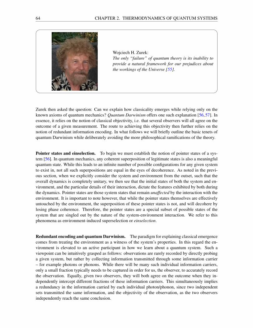
64 CHAPTER 2. THERMODYNAMICS OF QUANTUM SYSTEMS
Wojciech H. Zurek:The only “failure” of quantum theory is its inability toprovide a natural framework for our prejudices aboutthe workings of the Universe [55].
Zurek then asked the question: Can we explain how classicality emerges while relying only on theknown axioms of quantum mechanics? Quantum Darwinism offers one such explanation [56, 57]. Inessence, it relies on the notion of classical objectivity, i.e. that several observers will all agree on theoutcome of a given measurement. The route to achieving this objectivity then further relies on thenotion of redundant information encoding. In what follows we will briefly outline the basic tenets ofquantum Darwinism while deliberately avoiding the more philosophical ramifications of the theory.
Pointer states and einselection. To begin we must establish the notion of pointer states of a sys-tem [56]. In quantum mechanics, any coherent superposition of legitimate states is also a meaningfulquantum state. While this leads to an infinite number of possible configurations for any given systemto exist in, not all such superpositions are equal in the eyes of decoherence. As noted in the previ-ous section, when we explicitly consider the system and environment from the outset, such that theoverall dynamics is completely unitary, we then see that the initial states of both the system and en-vironment, and the particular details of their interaction, dictate the features exhibited by both duringthe dynamics. Pointer states are those system states that remain unaffected by the interaction with theenvironment. It is important to note however, that while the pointer states themselves are effectivelyuntouched by the environment, the superposition of these pointer states is not, and will decohere bylosing phase coherence. Therefore, the pointer states are a special subset of possible states of thesystem that are singled out by the nature of the system-environment interaction. We refer to thisphenomena as environment-induced superselection or einselection.
Redundant encoding and quantum Darwinism. The paradigm for explaining classical emergencecomes from treating the environment as a witness of the system’s properties. In this regard the en-vironment is elevated to an active participant in how we learn about a quantum system. Such aviewpoint can be intuitively grasped as follows: observations are rarely recorded by directly probinga given system, but rather by collecting information transmitted through some information carrier– for example photons or phonons. While there will be many such individual information carriers,only a small fraction typically needs to be captured in order for us, the observer, to accurately recordthe observation. Equally, given two observers, they will both agree on the outcome when they in-dependently intercept different fractions of these information carriers. This simultaneously impliesa redundancy in the information carried by each individual photon/phonon, since two independentsets transmitted the same information, and the objectivity of the observation, as the two observersindependently reach the same conclusion.
2.4. QUANTUM DECOHERENCE AND THE TALE OF QUANTUM DARWINISM 65
To illustrate how this can occur, let us assume the system is a qubit in the initial state
|ψS 〉= α |↑〉+β |↓〉 with |α|2 + |β |2 = 1, (2.97)
i.e. a superposition of the pointer states |↑〉 , |↓〉, and we assume the environment is a collection ofN qubits each written in the computational basis |0〉 , |1〉 all in the same initial state |ψEi〉. Thus,we start with an initially factorized state
|ψS E 〉i = (α |↑〉+β |↓〉)⊗|ψEi〉 . (2.98)
Quantum Darwinism then posits that, if after their mutual interaction, the total state of the sys-tem+environment is
|ψS E 〉= α |↑〉∣∣0⊗N⟩+β |↓〉
∣∣1⊗N⟩ . (2.99)
then classical objectivity emerges. The reason for this seemingly special form becomes apparentwhen we examine the reduced state of the system or the reduced state of any single environmentalunit. Taking the partial trace over the N environmental qubits we are left with the density matrix for S
ρS = |α|2| ↑〉〈↑ |+ |β |2| ↓〉〈↓ |. (2.100)
While for any single environment qubit we have
ρEi = |α|2|0〉〈0|+ |β |2|1〉〈1|. (2.101)
From Eq. (2.100) we see that after the interaction with the environment, the system state is left com-pletely decohered, and therefore in a classical state. Crucially however, the populations are unaf-fected. From Eq. (2.101) we see that every environmental qubit has resulted in the populations of thesystem becoming “imprinted” onto them. Therefore, by capturing a subset of the N environmentalqubits an observer is able to determine the state of the system. Equally a separate observer can capturea different subset of environmental qubits, and when both perform the same type of measurement ontheir respective sets, will necessarily arrive at the same conclusion. This is due to the entanglementshared between the system and all the environmental degrees of freedom. In fact, notice that after theirinteraction the system is maximally entangled with the environment. Indeed the states Eq. (2.99) areclosely related to those discussed in Sec. 1.3 where the foundations of statistical mechanics wherederived from quantum entanglement.
At this point it is important to revisit what we mean by objectivity. In the case of Eq. (2.99) it isclear that if each observer independently measures subsets of the environment they will gain the sameinformation about the system. In this respect it should be clear that objectivity will emerge when theamount of information learned about the system by interrogating portions of the environment exhibitsthis redundancy. Therefore, a key quantity in assessing quantum Darwinism is the mutual informationshared between the system, S , and the fraction of the environment which the observer is measuring,E f
IS E f = S(ρS )+S(ρE f )−S(ρS E f ), (2.102)
where S(·) is the von Neumann entropy, and ρ j are the appropriate reduced density matrices. We nowsee that the maximum IS E f = 2S(ρS ) and occurs when E f = E , i.e. the entire environment. Objec-tivity thus implies that for any other fraction of the environment, the amount of information shared bythe system, and therefore accessible to any observer measuring this fraction, will be IS E f = S(ρS ).Thus, quantum Darwinism is signalled by a characteristic plateau appearing in the behavior of IS E f
versus the fraction size. To show this is indeed the case, we consider the following example of asingle qubit undergoing decoherence within a spin-bath.
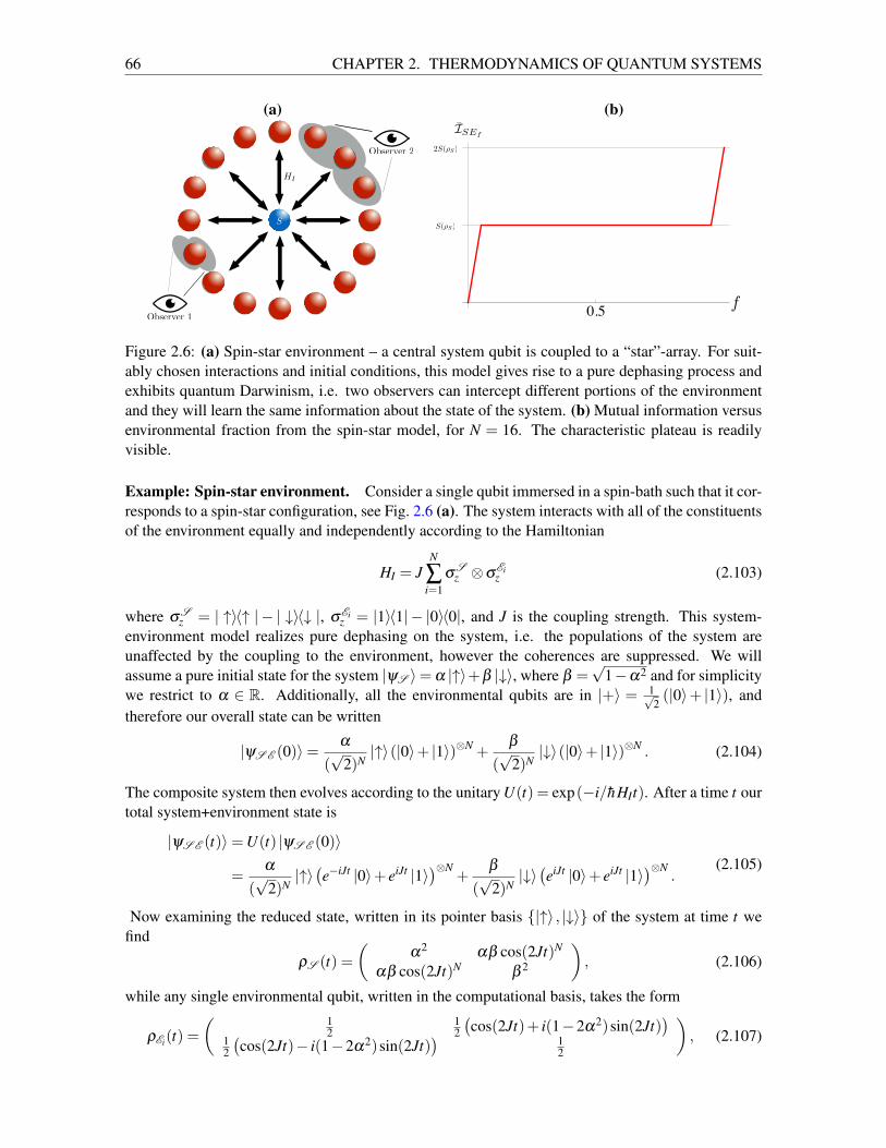
66 CHAPTER 2. THERMODYNAMICS OF QUANTUM SYSTEMS
(a) (b)
S
HI
Observer 1
Observer 2
0.5
S(S)
2S(S)
ISEf
f
Figure 2.6: (a) Spin-star environment – a central system qubit is coupled to a “star”-array. For suit-ably chosen interactions and initial conditions, this model gives rise to a pure dephasing process andexhibits quantum Darwinism, i.e. two observers can intercept different portions of the environmentand they will learn the same information about the state of the system. (b) Mutual information versusenvironmental fraction from the spin-star model, for N = 16. The characteristic plateau is readilyvisible.
Example: Spin-star environment. Consider a single qubit immersed in a spin-bath such that it cor-responds to a spin-star configuration, see Fig. 2.6 (a). The system interacts with all of the constituentsof the environment equally and independently according to the Hamiltonian
HI = JN
∑i=1
σSz ⊗σ
Eiz (2.103)
where σSz = | ↑〉〈↑ | − | ↓〉〈↓ |, σEi
z = |1〉〈1| − |0〉〈0|, and J is the coupling strength. This system-environment model realizes pure dephasing on the system, i.e. the populations of the system areunaffected by the coupling to the environment, however the coherences are suppressed. We willassume a pure initial state for the system |ψS 〉= α |↑〉+β |↓〉, where β =
√1−α2 and for simplicity
we restrict to α ∈ R. Additionally, all the environmental qubits are in |+〉 = 1√2(|0〉+ |1〉), and
therefore our overall state can be written
|ψS E (0)〉=α
(√
2)N|↑〉(|0〉+ |1〉)⊗N +
β
(√
2)N|↓〉(|0〉+ |1〉)⊗N . (2.104)
The composite system then evolves according to the unitary U(t) = exp(−i/hHIt). After a time t ourtotal system+environment state is
|ψS E (t)〉=U(t) |ψS E (0)〉
=α
(√
2)N|↑〉(e−iJt |0〉+ eiJt |1〉
)⊗N+
β
(√
2)N|↓〉(eiJt |0〉+ eiJt |1〉
)⊗N.
(2.105)
Now examining the reduced state, written in its pointer basis |↑〉 , |↓〉 of the system at time t wefind
ρS (t) =(
α2 αβ cos(2Jt)N
αβ cos(2Jt)N β 2
), (2.106)
while any single environmental qubit, written in the computational basis, takes the form
ρEi(t) =( 1
212
(cos(2Jt)+ i(1−2α2)sin(2Jt)
)12
(cos(2Jt)− i(1−2α2)sin(2Jt)
) 12
), (2.107)
2.4. QUANTUM DECOHERENCE AND THE TALE OF QUANTUM DARWINISM 67
When t = π/(4J) we find that the overall system+environment state, Eq. (2.105) has the same generalform as given in Eq. (2.99) and furthermore that the system (and any environmental qubit) is fully de-cohered. We now consider the information that an observer can learn about the system by measuringsome fraction, f = n/N, of the environment. It is a matter of direct calculation to find that regardlessof the size of the environmental fragment the observer interrogates, the mutual information sharedbetween the system and the environment will be IS E f = S(ρS ). In Fig. 2.6 we show the charac-teristic “plateau” signalling the redundant encoding of information about the system throughout theenvironment.
68 CHAPTER 2. THERMODYNAMICS OF QUANTUM SYSTEMS
2.5 Checklist for “Thermodynamics of Quantum Systems”
1. Measuring low temperatures is not as simple as just sticking a thermometer into a quantumsystem.
2. Quantum systems with maximal energy variance, and therefore heat capacity, are the optimalthermometers.
3. Reversible Otto engines with quantum working fluids achieve the same efficiency as their clas-sical counterparts.
4. Quantum working fluids allow to go beyond the Curzon-Ahlborn efficiency at maximum powerfor endoreversible Otto cycles.
5. Work may be extracted from multiple copies of a passive, but not completely passive, quantumbattery by performing entangling operations.
6. Dynamical generation of entanglement leads to a significant boost in the charging power ofarrays of quantum batteries.
7. Entropy production can be understood as the correlations established between the system andits environment.
8. Quantum Darwinism provides a framework to explain classical objectivity through ‘redundantencoding’, i.e. imprinting the same system information onto multiple environment degrees offreedom.
2.6 Problems
Quantum thermometry 2.1
[1] A spin-1 particle is found in a thermal state at temperature T . Compute the quantum Fisherinformation for the corresponding state. At optimal precision, can the temperature be estimatedmore accurately for spin-1/2 particles or spin-1 particles?
[2] Consider two quantum two-level systems (TLS). In which situation can the temperature bemeasured more precisely: (i) if the two TLS are non-interacting and independently prepared attemperature T ; or (ii) if the two TLS interact as described by the quantum Ising model in thetransverse field?
Quantum heat engines – engines with atomic working fluids 2.2
[3] Consider a quantum Otto engine operating on a working medium with Hamiltonian,
H(t) =−µ~S ·~B(t) ,
where ~S = (Sx,Sy,Sz) describes a spin-1 particle, i.e.,
Sx =h√2
0 1 01 0 10 1 0
, Sy =i h√
2
0 −1 01 0 −10 1 0
, and Sz =h√2
1 0 00 0 00 0 −1
.
Compute its efficiency for quasistatic variation of the magnetic field.
2.6. PROBLEMS 69
[4] The entropy of a semiclassical, ideal gas is given by the Sackur-Tetrode equation,
S(E,V,N) = NkB
[52+ ln
(V
Nh3
(4πmE
3N
)(3/2))]
.
What is the (endoreversible) efficiency at maximal power of an Otto engine operating with sucha semiclassical gas as working medium?
Work extraction from quantum systems 2.3
[5] Consider again a spin-1 particle with Hamiltonian
H =−µ~S ·~B ,
where as before ~S = (Sx,Sy,Sz) is given by
Sx =h√2
0 1 01 0 10 1 0
, Sy =i h√
2
0 −1 01 0 −10 1 0
, and Sz =h√2
1 0 00 0 00 0 −1
.
Determine the maximal ergotropy with respect to the completely passive state that can be storedin any quantum state ρ as a function of temperature T .
[6] A specific quantum battery consists of an array of n qubits. Compute the maximal ergotropywith respect to the completely passive state as a function of T that can stored in such a battery.
Quantum decoherence and the tale of quantum Darwinism 2.4
[7] A quantum system undergoes “pure” decoherence in the energy basis if the master equationtakes the form
dρ
dt=− i
h[H, ρ]−∑
i6= jγi, j |i〉〈 j| ,
where |i〉 is an energy eigenstate and γi, j are the coefficients of the coupling matrix. Showthat this master equation can be brought into Lindblad form and that the resulting dynamics isunital.
[8] Consider the reduced two qubit state, ρSEi , consisting of a system qubit, S, and any singleenvironmental qubit, Ei, taken from a larger environment of the form
ρSEi = p|φ〉〈φ |+(1− p)|ψ〉〈ψ|
where |φ〉 = √p |00〉+√1− p |11〉, |ψ〉 = √p |01〉+√1− p |10〉 and p 6= 1/2. Determinethe marginal states, entropies, and the mutual information, and therefore show that the stateof S is objective according to quantum Darwinism. Is this state entangled? If so, what doesthis imply about the validity and applicability of defining classical objectivity through quantumDarwinism?
References
[1] O. Abah, J. Roßnagel, G. Jacob, S. Deffner, F. Schmidt-Kaler, K. Singer, and E. Lutz. Single-ionheat engine at maximum power. Phys. Rev. Lett., 109:203006, 2012.
[2] R. Alicki. The quantum open system as a model of the heat engine. J. Phys. A: Math. Gen.,12:L103, 1979.
[3] R. Alicki and M. Fannes. Entanglement boost for extractable work from ensembles of quantumbatteries. Phys. Rev. E, 87:042123, 2013.
[4] A. E. Allahverdyan, R. Balian, and Th. M. Nieuwenhuizen. Maximal work extraction fromfinite quantum systems. EPL (Europhysics Letters), 67:565, 2004.
[5] F. C Binder, S. Vinjanampathy, K. Modi, and J. Goold. Quantacell: powerful charging ofquantum batteries. New J. Phys., 17:075015, 2015.
[6] H.-P Breuer and F. Petruccione. The theory of open quantum systems. Oxford, 2002.
[7] H. Callen. Thermodynamics and an Introduction to Thermostastistics. Wiley, New York, USA,1985.
[8] F. Campaioli, F. A. Pollock, F. C. Binder, L. Celeri, J. Goold, S. Vinjanampathy, and K. Modi.Enhancing the charging power of quantum batteries. Phys. Rev. Lett., 118:150601, 2017.
[9] S. Campbell, M. G. Genoni, and S. Deffner. Precision thermometry and the quantum speedlimit. Quantum Sci. Technol., 3:025002, 2018.
[10] L. A. Correa, M. Mehboudi, G. Adesso, and A. Sanpera. Individual quantum probes for optimalthermometry. Phys. Rev. Lett., 114:220405, 2015.
[11] F. L. Curzon and B. Ahlborn. Efficiency of a Carnot engine at maximum power output. Am. J.Phys., 43:22, 1975.
[12] A. De Pasquale, D. Rossini, R. Fazio, and V. Giovannetti. Local quantum thermometry. Nat.Commun., 7:12782, 2016.
[13] S. Deffner. Efficiency of harmonic quantum otto engines at maximal power. Entropy, 20:875,2018.
[14] S. Deffner and S. Campbell. Quantum speed limits: from Heisenberg’s uncertainty principle tooptimal quantum control. J. Phys. A: Math. Theor., 50:453001, 2017.
[15] A. del Campo, J. Goold, and M. Paternostro. More bang for your buck: Towards super-adiabaticquantum engines. Sci. Rep., 4:6208, 2014.
70
REFERENCES 71
[16] L. B. Erbay and H. Yavuz. Analysis of the Stirling heat engine at maximum power conditions.Energy, 22:645, 1997.
[17] M. Esposito, K. Lindenberg, and C. Van den Broeck. Entropy production as correlation betweensystem and reservoir. New J. Phys., 12:013013, 2010.
[18] D. Ferraro, M. Campisi, G. M. Andolina, V. Pellegrini, and M. Polini. High-power collectivecharging of a solid-state quantum battery. Phys. Rev. Lett., 120:117702, 2018.
[19] B. Gardas and S. Deffner. Thermodynamic universality of quantum Carnot engines. Phys. Rev.E, 92:042126, 2015.
[20] J. Gemmer, M. Michel, and G. Mahler. Quantum Thermodynamics. Springer, Berlin / Heidel-berg, 2009.
[21] G. L. Giorgi and S. Campbell. Correlation approach to work extraction from finite quantumsystems. J. Phys. B: At. Mol. Opt. Phys., 48:035501, 2015.
[22] A. U. C. Hardal and O. E. Mustecaploglu. Superradiant quantum heat engine. Sci. Rep., 5:12953,2015.
[23] Carl W. Helstrom. Quantum Detection and Estimation Theory. Academic Press, New York,1976.
[24] K. V. Hovhannisyan, M. Perarnau-Llobet, M. Huber, and A. Acın. Entanglement generation isnot necessary for optimal work extraction. Phys. Rev. Lett., 111:240401, 2013.
[25] J. Klaers, S. Faelt, A. Imamoglu, and E. Togan. Squeezed thermal reservoirs as a resource for ananomechanical engine beyond the Carnot limit. Phys. Rev. X, 7:031044, 2017.
[26] R. Kosloff and Y. Rezek. The Quantum Harmonic Otto Cycle. Entropy, 19:136, 2017.
[27] H. S. Leff. Thermal efficiency at maximum work output: New results for old heat engines. Am.J. Phys., 55:602, 1987.
[28] G. Lindblad. Completely positive maps and entropy inequalities. Comm. Math. Physics, 40:147,1975.
[29] S. Marcantoni, S. Alipour, F. Benatti, R. Floreanini, and A. T. Rezakhani. Entropy productionand non-markovian dynamical maps. Sci. Rep., 7:12447, 2017.
[30] M. Mehboudi, A. Sanpera, and L. A. Correa. Thermometry in the quantum regime: Recenttheoretical progress. arXiv:1811.03988, 2018.
[31] A. Muller-Hermes and D. Reeb. Monotonicity of the quantum relative entropy under positivemaps. Annales Henri Poincare, 18:1777, 2017.
[32] P. Naze and M. V. S. Bonanca. Compatibility of linear-response theory with the second law ofthermodynamics and the emergence of negative entropy production rates. arXiv:1902.10217,2019.
[33] W. Niedenzu, V. Mukherjee, A. Ghosh, A. G. Kofman, and G. Kurizki. Quantum engine effi-ciency bound beyond the second law of thermodynamics. Nat. Commun., 9:165, 2018.
[34] M. G. A. Paris. Quantum estimation for quantum technology. Int. J. Quant. Inf., 07:125, 2009.
72 REFERENCES
[35] M. G. A. Paris. Achieving the Landau bound to precision of quantum thermometry in systemswith vanishing gap. J. Phys. A: Math. Theor., 49:03LT02, 2016.
[36] M. Popovic, B. Vacchini, and S. Campbell. Entropy production and correlations in a controllednon-Markovian setting. Phys. Rev. A, 98:012130, 2018.
[37] W. Pusz and S. L. Woronowicz. Passive states and KMS states for general quantum systems.Commun. Math. Phys., 58:273, 1978.
[38] H. T. Quan, Y.-X. Liu, C. P. Sun, and F. Nori. Quantum thermodynamic cycles and quantumheat engines. Phys. Rev. E, 76:031105, 2007.
[39] H. T. Quan, P. Zhang, and C. P. Sun. Quantum heat engine with multilevel quantum systems.Phys. Rev. E, 72:056110, 2005.
[40] Y. Rezek and R. Kosloff. Irreversible performance of a quantum harmonic heat engine. New J.Phys., 8:83, 2006.
[41] A. Ronzani, B. Karimi, J. Senior, Y.-C. Chang, J. T. Peltonen, C. Chen, and J. P. Pekola. Tunablephotonic heat transport in a quantum heat valve. Nat. Phys., 14:991, 2018.
[42] J. Roßnagel, O. Abah, F. Schmidt-Kaler, K. Singer, and E. Lutz. Nanoscale heat engine beyondthe carnot limit. Phys. Rev. Lett., 112:030602, 2014.
[43] J. Roßnagel, S. T. Dawkins, K. N. Tolazzi, O. Abah, E. Lutz, F. Schmidt-Kaler, and K. Singer.A single-atom heat engine. Science, 352:325, 2016.
[44] A. Roulet, S. Nimmrichter, and J. M. Taylor. An autonomous single-piston engine with a quan-tum rotor. Quantum Sci. Technol., 3:035008, 2018.
[45] B. C. Sanders. How to Build a Quantum Computer. 2399. IOP Publishing, 2017.
[46] H. E. D. Scovil and E. O. Schulz-DuBois. Three-level masers as heat engines. Phys. Rev. Lett.,2:262, 1959.
[47] M. O. Scully. Quantum afterburner: Improving the efficiency of an ideal heat engine. Phys. Rev.Lett., 88:050602, 2002.
[48] M. O. Scully, K. R. Chapin, K. E. Dorfman, M. B. Kim, and A. Svidzinsky. Quantum heatengine power can be increased by noise-induced coherence. PNAS, 108:15097, 2011.
[49] M. O. Scully, M. S. Zubairy, G. S. Agarwal, and H. Walther. Extracting work from a single heatbath via vanishing quantum coherence. Science, 299:862, 2003.
[50] H. Spohn. Entropy production for quantum dynamical semigroups. J. Math. Phys., 19:1227,1978.
[51] H. Spohn and J. L. Lebowitz. Irreversible Thermodynamics for Quantum Systems WeaklyCoupled to Thermal Reservoirs. Adv. Chem. Phys., XXXVIII:109, 1978.
[52] P. Strasberg and M. Esposito. Non-markovianity and negative entropy production rates. Phys.Rev. E, 99:012120, 2019.
[53] P. Zanardi, M. G. A. Paris, and L. Campos Venuti. Quantum criticality as a resource for quantumestimation. Phys. Rev. A, 78:042105, 2008.
REFERENCES 73
[54] K. Zhang, F. Bariani, and P. Meystre. Quantum optomechanical heat engine. Phys. Rev. Lett.,112:150602, 2014.
[55] W. H. Zurek. Decoherence and the transition from quantum to classical. Phys. Tod., 44:36,1991.
[56] W. H. Zurek. Decoherence, einselection, and the quantum origins of the classical. Rev. Mod.Phys., 75:715, 2003.
[57] W. H. Zurek. Quantum Darwinism. Nat. Phys., 5:181, 2009.
Chapter 3
Thermodynamics of QuantumInformation
The phrase quantum supremacy typically refers to situations in which information processing devicesbuilt on the principles of quantum physics solve computational problems that are not tractable byclassical computers [60]. The resulting quantum advantage is the ratio of classical resources, suchas time or memory, to the associated quantum resources. Generally, the hardware requirements toachieve this computational supremacy can be summarized by three key properties [47] (i) the quantumsystems must initially be prepared in a well-defined state; (ii) arbitrary unitary operators must beavailable and controllable in order to launch an arbitrary entangled state; and (iii) measurements ofthe qubits must be performed with high quantum efficiency.
As we have already discussed, however, all physical quantum systems are subject to decoherenceand dissipation arising from their noisy interaction with the environment. Thus, thermodynamicallyspeaking any realistic operation of quantum information processing devices will be accompanied bythe production of irreversible entropy, and by the irretrievable loss of quantum information into theenvironment.
In the present context, some questions appear immediate: how can the tools and techniques ofquantum thermodynamics help to optimally operate quantum computers, i.e., how can we keep quan-tum computers in the deep quantum regime so that we can actually utilize their supremacy? In thischapter, we will quantify the thermodynamic cost of quantum information processing in Sec. 3.1.Then, Sec. 3.2 is dedicated to assessing the performance of adiabatic quantum computers by meansof Quantum Stochastic Thermodynamics. This will turn our attention to thermodynamic propertiesof critical systems. Specifically, in Sec. 3.3 we assess the Kibble-Zurek mechanism of defect forma-tion and its relation with the irreversible entropy production. Such an analysis is particularly relevantin certain quantum computational platforms, particularly those that rely on annealing. We close thechapter with a brief outline on recent efforts in developing quantum error correcting schemes foradiabatic quantum computers in Sec. 3.4.
3.1 Quantum thermodynamics of information
3.1.1 Thermodynamics of classical information processing
Information is physical. This is the conclusion established by Rolf Landauer in his landmark 1961paper [42]. The question posed was relatively simple: What are the physical limitations on infor-mation processing set by the laws of thermodynamics? As has been widely noted since, and evenacknowledged by Landauer himself in the original paper, the notion of an energetic price to pay for
74
3.1. QUANTUM THERMODYNAMICS OF INFORMATION 75
processing information is not surprising, after all information is encoded in physical systems andtherefore must be subject to the laws of thermodynamics. Indeed any process occurring at a finiterate will be accompanied by some dissipation. What was remarkable about Landauer’s insight wasthat it established an absolute minimum cost, independent of any other constraints, that must be paidto erase information. Thus showing that, far from being an abstract concept, information truly is asphysical as any other quantity. Among the many consequences of Landauer’s principle, probably themost famous is the exorcism of Maxwell’s Demon [8]. However, another notable consequence wasthe theoretical proposals for fully reversible models of computation [7]. There are many subtleties inunderstanding Landauer’s insight, therefore to begin we shall discuss the basic motivations that leadto the result.
Landauer, Bennett, and the famous kBT ln2. To first gain an intuitive picture, consider the opera-tion that restores a bit to a given state, say 1. If the state of the bit is initially known then there willbe two possible procedures to achieve this: either the bit is already in 1 and we do nothing, or thebit is initially in 0 and we must change it to 1. Notice that regardless, in both of these settings theentropy of the bit is left unchanged since it always begins and ends in a definite state, thus has zeroentropy. Both of these operations can be done, in principle, in a fully reversible manner and thereforecorrespond to no “wasted” energy being dissipated. However, it is clear that this is not how a normalinformation processing device works, as such devices will operate on data that is independent of theparticular process or computation it is performing.
Therefore, Landauer asks the question whether there exists some process that can always performthe action restore to 1, regardless of the state that the bit is in, without dissipating heat. If we con-sider the two processes mentioned already, since they are both reversible we can imagine runningthem backwards in time. Now we see the problem: by definition the individual processes are fullydeterministic, however in the time-reversed scenario we have a single initial condition, the bit in 1,but two possible final states. Therefore, there cannot be a conservative force that always restores thebit to 1 regardless of its initial state. This is the basic reasoning that Landauer followed to show thatinformation erasure comes at an inescapable thermodynamic cost.
Indeed, in the above reasoning we clearly see that two possible inputs lead to a single output, andtherefore we can define the notion of logical irreversibility as those processes which the output doesnot uniquely define the inputs. This form of irreversibility is common in most computing devices,the AND gate is an example of a logically irreversible gate, as its two inputs that lead to a singleoutput. However, such irreversible operations can be avoided, either by saving the entire history ofthe process, or by embedding the usual irreversible gate operations, such as the AND, into morecomplex but reversible gate operations, e.g. using a Toffoli gate. This is a remarkable observation asit indicates that the processing of information has no intrinsic thermodynamic cost.
How then do we arrive at Landauer’s principle? First we must examine a subtle difference be-tween information copying and information erasure. For a single bit in a given state, we can faithfullycopy this bit onto a blank bit in a fully reversible manner. This is clear as it is a one-to-one process.This can again be seen by considering the entropy before and after the copying procedure: both bitshave definite states before and after, and therefore the entropy is constant and zero. The subtletyarises when we consider erasure of a bit of information. In this case we have two possible statesbeing mapped to a single definite state. Landauer’s principle states that: the entropy decrease of theinformation bearing degrees of freedom must be compensated by an equal or greater entropy increasein the environment.
For a two-state system containing a bit of information the initial Shannon entropy, G=−∑i pi ln pi,which quantifies its information content, is ln2. After the erasure the entropy is zero. If our systembit, S , is surrounded by a large thermal reservoir, E , in equilibrium at temperature T , from the second
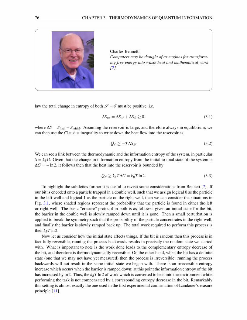
76 CHAPTER 3. THERMODYNAMICS OF QUANTUM INFORMATION
Charles Bennett:Computers may be thought of as engines for transform-ing free energy into waste heat and mathematical work[7].
law the total change in entropy of both S +E must be positive, i.e.
∆Stot = ∆SS +∆SE ≥ 0. (3.1)
where ∆S = Sfinal− Sinitial. Assuming the reservoir is large, and therefore always in equilibrium, wecan then use the Clausius inequality to write down the heat flow into the reservoir as
QE ≥−T ∆SS (3.2)
We can see a link between the thermodynamic and the information entropy of the system, in particularS = kBG. Given that the change in information entropy from the initial to final state of the system is∆G =− ln2, it follows then that the heat into the reservoir is bounded by
QE ≥ kBT ∆G = kBT ln2. (3.3)
To highlight the subtleties further it is useful to revisit some considerations from Bennett [7]. Ifour bit is encoded onto a particle trapped in a double well, such that we assign logical 0 as the particlein the left-well and logical 1 as the particle on the right-well, then we can consider the situations inFig. 3.1, where shaded regions represent the probability that the particle is found in either the leftor right well. The basic “erasure” protocol in both is as follows: given an initial state for the bit,the barrier in the double well is slowly ramped down until it is gone. Then a small perturbation isapplied to break the symmetry such that the probability of the particle concentrates in the right well,and finally the barrier is slowly ramped back up. The total work required to perform this process isthen kBT ln2.
Now let us consider how the initial state affects things. If the bit is random then this process is infact fully reversible, running the process backwards results in precisely the random state we startedwith. What is important to note is the work done leads to the complementary entropy decrease ofthe bit, and therefore is thermodynamically reversible. On the other hand, when the bit has a definitestate (one that we may not have yet measured) then the process is irreversible: running the processbackwards will not result in the same initial state we began with. There is an irreversible entropyincrease which occurs when the barrier is ramped down; at this point the information entropy of the bithas increased by ln2. Thus, the kBT ln2 of work which is converted to heat into the environment whileperforming the task is not compensated by a corresponding entropy decrease in the bit. Remarkablythis setting is almost exactly the one used in the first experimental confirmation of Landauer’s erasureprinciple [11].
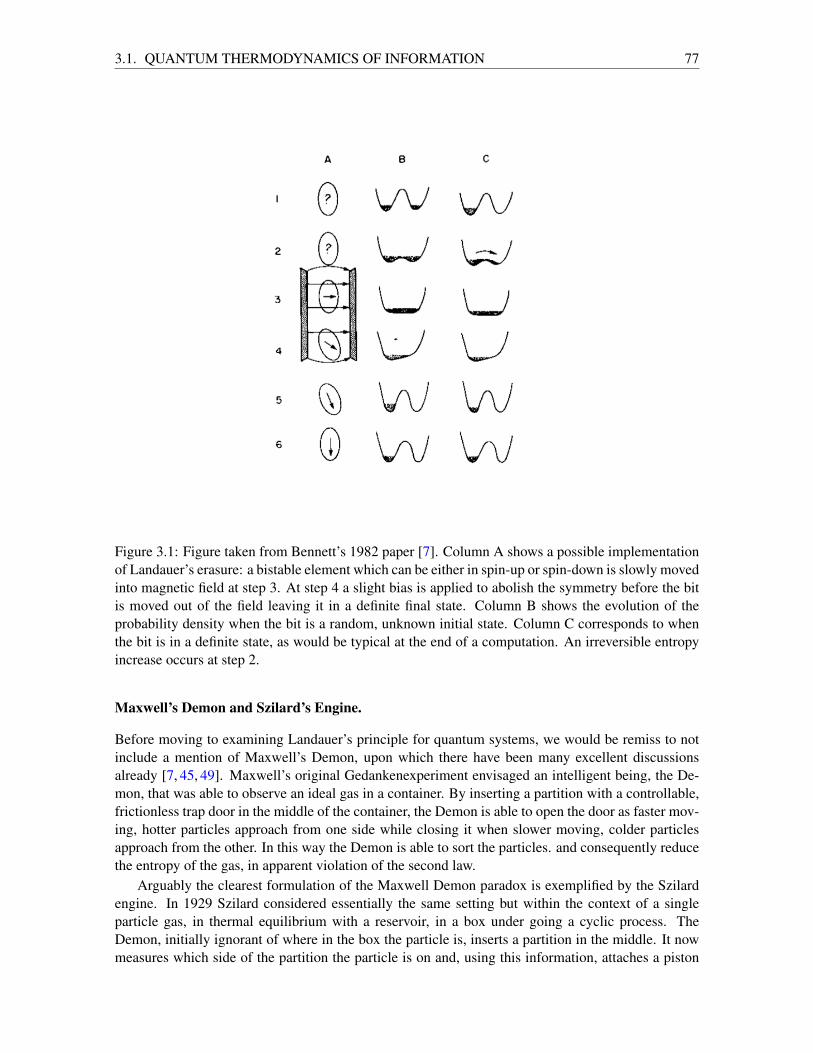
3.1. QUANTUM THERMODYNAMICS OF INFORMATION 77
Figure 3.1: Figure taken from Bennett’s 1982 paper [7]. Column A shows a possible implementationof Landauer’s erasure: a bistable element which can be either in spin-up or spin-down is slowly movedinto magnetic field at step 3. At step 4 a slight bias is applied to abolish the symmetry before the bitis moved out of the field leaving it in a definite final state. Column B shows the evolution of theprobability density when the bit is a random, unknown initial state. Column C corresponds to whenthe bit is in a definite state, as would be typical at the end of a computation. An irreversible entropyincrease occurs at step 2.
Maxwell’s Demon and Szilard’s Engine.
Before moving to examining Landauer’s principle for quantum systems, we would be remiss to notinclude a mention of Maxwell’s Demon, upon which there have been many excellent discussionsalready [7, 45, 49]. Maxwell’s original Gedankenexperiment envisaged an intelligent being, the De-mon, that was able to observe an ideal gas in a container. By inserting a partition with a controllable,frictionless trap door in the middle of the container, the Demon is able to open the door as faster mov-ing, hotter particles approach from one side while closing it when slower moving, colder particlesapproach from the other. In this way the Demon is able to sort the particles. and consequently reducethe entropy of the gas, in apparent violation of the second law.
Arguably the clearest formulation of the Maxwell Demon paradox is exemplified by the Szilardengine. In 1929 Szilard considered essentially the same setting but within the context of a singleparticle gas, in thermal equilibrium with a reservoir, in a box under going a cyclic process. TheDemon, initially ignorant of where in the box the particle is, inserts a partition in the middle. It nowmeasures which side of the partition the particle is on and, using this information, attaches a piston
78 CHAPTER 3. THERMODYNAMICS OF QUANTUM INFORMATION
to the side of the partition not containing the particle. The expansion of the particle then leads tokBT ln2 of work being extracted. At the end of the process the only record of where the particle waswhen the partition was introduced is in the Demon’s memory. Thus, it was often believed that it wasthe act of measurement that accounted for the discrepancy.
Once again, Bennett, using the insight from Landauer’s principle, clarified that it is actually theerasure the Demon’s memory that restores the second law. To see this, consider a Demon with amemory that can be in three possible states, left (L), right (R), and standard (S). Assuming it starts inS, after inserting the partition, the act of measurement is similar to copying the single bit informationabout where the particle is to the Demon’s memory. As already discussed, the copying of informa-tion comes at no intrinsic thermodynamic cost. However, evidently to close the cycle the Demon’smemory must be returned to the standard state, i.e. the information about which side of the parti-tion the particle was on must be erased which, from Landauer’s principle, leads to the correspondingdissipation of kBT ln2 of heat. While the inclusion of the standard state for the Demon’s memory isnot crucial (a similar argument can be followed for a memory with only two possible states), it doesgreatly help in identifying erasure as the source of the apparent paradox and not the measurementprocess [7].
3.1.2 A quantum sharpening of Landauer’s bound
Interestingly Landauer’s principle as considered above appeared to largely apply in the quantum do-main, however only recently has the statement been made more mathematically rigorous. The state-ment of Landauer’s principle can be made more concrete by first establishing a minimal set of con-ditions for which the notion of information erasure has a definite meaning. To this end, consider asystem S whose information content we want to erase by making it interact with an environment E .Following Landauer’s own reasoning [42], Reeb and Wolf determined that the following constitute aminimal set of assumptions, which ensure the validity of Landauer’s principle [53], and apply to bothclassical and quantum settings:
1. Both S and E are quantum systems, living in Hilbert spaces HS and HE respectively;
2. The initial state of the composite system is factorized, i.e. ρS E (0) = ρS (0)⊗ρE (0), such thatno initial correlations are present;
3. The environment is prepared in the thermal state ρE (0) = ρβ = exp(−βHE )/ZE with HE theHamiltonian of the environment, which we spectrally decompose as
HE = ∑m
Em |Em〉〈Em|= ∑m
EmΠm.
Here, |Em〉 is the mth eigenstate of HE , associated with eigenvalue Em. Finally, we have intro-duced the partition function ZE = trE exp(−βHE );
4. System and environment interact via the overall unitary transformation U(t) = exp(−iHt/h)with H = HS +HE +HS E the total Hamiltonian.
Assumptions 1 and 3 are well motivated: one must be able to clearly partition our overall systemso as to (initially) be able to unambiguously identify the system and environment. Furthermore, therequirement for an initially thermal state of the reservoir is also physically well motivated, recall fromSec. 2.3 that thermal states are the only completely passive states. Thus, if the environment is in anyother state it would be possible to violate Landauer’s principle. Regarding assumption 2, as has beenextensively used throughout this book, the initially factorized state is common in thermodynamics,
3.1. QUANTUM THERMODYNAMICS OF INFORMATION 79
and in fact is required for Landauer’s principle to hold: if S and E share some initial correlationsthen it can be shown that the system entropy can be reduced without a corresponding increase inthe environment. Finally, assumption 4 is required to ensure that no auxiliary environment can beinvolved in the evolution, and therefore all resources used during the process are fully taken intoaccount.
Using only these assumptions, we can derive a rigorous equality version of Landauer’s principle.First let us carefully set some notation. Landauer’s principle is related to the change in entropy of thesystem, therefore we will denote an entropy change for the system/reservoir as the difference betweentheir initial and final entropies1
∆SS (E ) = S(ρ0S (E ))−S(ρ t
S (E )). (3.4)
Notice that these entropy changes can be positive or negative. To establish Landauer’s principle, wefirst consider the entropy production of the process, i.e. the difference between the final and initialentropies, which according to the second law must be positive
−∆SS −∆SE = S(ρ tS )−S(ρ0
S )+S(ρ tE )−S(ρ0
E )
= S(ρ tS )+S(ρ t
E )−S(ρ0S ⊗ρ
0E )
= S(ρ tS )+S(ρ t
E )−S(ρ tS E )
= I(ρ tS E )≥ 0,
(3.5)
i.e. the mutual information shared between system and reservoir at the end of the process. In movingfrom the second to the third line we have used the invariance of the von Neumann entropy underunitary transformations. From the non-negativity of the mutual information, it follows that this is astatement of the second law.
Simply rearranging Eq. (3.5) we have
I(ρ tS E )+∆SS =−∆SE
=−tr
ρtE lnρ
tE
+ tr
ρ
0E ln
[e−βHE
tr
e−βHE]
=−tr
ρtE lnρ
tE
−β tr
HE ρ
0E
− ln tr
e−βHE
+β tr
HE ρ
tE
−β tr
HE ρ
tE
= β tr
HE
(ρ
tE −ρ
0E
)− tr
ρ
tE lnρ
tE
+ tr
ρ
tE lnρ
0E
= β 〈QE 〉−S(ρ t
E ‖ρ0E )
(3.6)
Therefore the following equality follows [29, 53]
β 〈QE 〉= ∆SS + I(ρ tS E )+S(ρ t
E ‖ρ0E ), (3.7)
which is the equality version of Landauer’s principle, valid for non-equilibrium settings. As both therelative entropy and the mutual information are non-negative functions, we can arrive at Landauer’sbound by simply dropping them to give
β 〈QE 〉 ≥ ∆SS , (3.8)
which is the non-equilibrium (quantum) Landauer’s principle. Notice that Eq. (3.7) is in fact equiva-lent to the expression for entropy production derived in Sec. 2.4.1 Eq. (2.95). Reeb and Wolf’s resulthas a further interesting consequence: equality in Landauer’s bound holds only for trivial processes,i.e. those that in essence do nothing [53].
1It is important to note that Reeb and Wolf’s rigorous treatment relate the change in entropy between initial and finalsystem states with the heat transferred to the reservoir, while the more ‘intuitive’ derivation in Sec. 3.1.1 employed theentropy production.
80 CHAPTER 3. THERMODYNAMICS OF QUANTUM INFORMATION
3.1.3 New Landauer bounds for non-equilibrium quantum systems
Beyond the clear conceptional milestone that Landauer’s insight provided, recently some efforts havegone into exploring and extending the idea of Landauer’s bound [36,37]. Indeed Landauer’s principle,in its most basic reading, is simply a lower bound on the dissipated heat. In the previous section wehave established that the change in information entropy provides a perfectly valid non-equilibriumlower bound to the dissipated heat. Here we examine an alternative method originally published inRef. [37] to lower bound the dissipated heat that, rather than relying on the information change, isinstead derived by applying the two-time energy measurement protocol from Sec. 1.4.3.
Full counting statistics approach to dissipated heat. We can use the full counting statistics of theheat dissipated by the system (which corresponds to the change in environmental energy [29, 53]) toaccess its mean value. Consider the same two-time energy measurement protocol for determiningthe quantum work introduced in Sec. 1.4.3. The heat probability distribution, P(QE ), to record atransferred amount of heat QE , can be formally defined in the same manner. In line with the minimalassumptions for Landauer’s principle to be applicable, we assume S to be initially uncorrelated withE , which is prepared in an equilibrium state. Therefore ρS E (0) = ρS (0)⊗ρβ with
[HE ,ρβ
]= 0.
Now we apply the two-time energy measurement approach to the environment: A projection over oneof the energy eigenstates of the environment at time t = 0 is carried out, obtaining En as an outcome.As a result, the total S -E state is
ρ′S E (0) = ρS (0)⊗Πn. (3.9)
Immediately after the measurement, the interaction between S and E is switched on and the overallsystem undergoes a joint evolution up to a generic time t, when the interaction is switched off anda second projective measurement of the environmental energy is performed, this time obtaining anoutcome Em. After the second measurement, we have
ρ′′S E (t) =
ΠmU(t)ρ ′S E (0)U(t)†Πm
trS E
ΠmU(t)ρ ′S E (0)U(t)†
. (3.10)
It is worth stressing that the set of assumptions and steps used in the two-time measurement protocolare perfectly compatible with those required by the erasure process. The joint probability to haveobtained the two stated outcomes at times 0 and t respectively is given by the Born rule
p(|n〉 → |m〉) = tr
ΠmU(t)ΠnρS (0)⊗ρβ ΠnU†(t)Πm, (3.11)
from which the probability distribution P(QE ) follows as
P(QE ) = ∑n,m
δ (QE − (Em−En))p(|n〉 → |m〉). (3.12)
The cumulant generating function is defined as the Laplace transform of the probability distribution
Θ(η ,β , t)≡ ln〈e−ηQE 〉= ln∫
dQE P(QE )e−ηQE , (3.13)
which can be seen as the Wick rotated version of the usual definition given by the Fourier transformof P(QE ). The cumulant of nth order is simply obtained by differentiation with respect to the realparameter η as
〈QnE 〉= (−1)n ∂ n
∂ηn Θ(η ,β , t)|η=0. (3.14)
3.2. PERFORMANCE DIAGNOSTICS OF QUANTUM ANNEALERS 81
Note that in the definition of the cumulant generating function we have explicitly written the depen-dence on the inverse temperature β of the bath, which enters in the joint probability Eq. (3.11) throughthe initial environmental state ρβ . The crucial point in using the full counting statistics approach isthat the cumulant generating function introduced in Eq. (3.13) can be expressed as
Θ(η ,β , t) = ln(trS ρS (η ,β , t)
), (3.15)
whereρS (η ,β , t) = trE
Uη/2(t)ρS (0)⊗ρβU†
η/2(t), (3.16)
with Uη/2(t) ≡ e−(η/2)HE U(t)e(η/2)HE . By invoking the same approximations and techniques usedto derive a master equation for the density matrix of the system ρS (t) [14], one can obtain a newequation for ρS (η ,β , t). Solving this is a task with the same degree of complexity as accessing thedynamics of the reduced system. However we may circumvent this difficulty by deriving a family oflower bounds to 〈QE 〉 using the counting statistics arising from the two-time measurement protocol.
Lower bounds on the mean dissipated heat. In order to derive a lower bound for 〈QE 〉, weconsider the cumulant generating function of its probability distribution. Having it defined as inEq. (3.13), we can apply Holder’s inequality to prove that Θ(η ,β , t) is a convex function with respectto the counting parameter η . This condition can be equivalently expressed as
Θ(η ,β , t)≥ η∂
∂ηΘ(η ,β , t)
∣∣η=0. (3.17)
Combining Eq. (3.14) and Eq. (3.17), we obtain a one-parameter family of lower bounds for the meandissipated heat 〈QE 〉 leading to
β 〈QE 〉 ≥ −β
ηΘ(η ,β , t)≡Bη
QE(t) (η > 0). (3.18)
As with Eq. (3.8), Eq. (3.18) is valid in the case of a generic erasure protocol. It is worth notinghowever that the two bounds arise from totally different underlying frameworks, the former rooted inan information approach while the latter takes a more thermodynamic take on the problem, as suchtheir performance as meaningful bounds to the dissipated heat in a given non-equilibrium setting hasbeen shown to be quite different [19].
3.2 Performance diagnostics of quantum annealers
In the preceding sections we have seen that purely quantum resources can lead to a modification of thestatements of thermodynamics. This is due to the additional (quantum) informational contribution tothe entropy production. The natural question arises whether these generalized statements can be usedin a practically relevant situation to teach us something about the quantum information processingsystem that we would not have known otherwise. That this is, indeed, the case has been shown byusing the generalized quantum fluctuation theorem (1.126) to assess the performance of adiabaticquantum computers [34].
Adiabatic quantum computing is a distinct paradigm of quantum computing [30], that relies onquantum annealing [40]. In quantum annealing a quantum system is initially prepared in the groundstate of a simple and controllable Hamiltonian. Then, the Hamiltonian is slowly varied, such that thesystem remains in the instantaneous ground state at all times. According to the quantum adiabatictheorem “slow” means that the rate with the Hamiltonian changes is much smaller than one over the
82 CHAPTER 3. THERMODYNAMICS OF QUANTUM INFORMATION
energy gap between instantaneous ground state and first excited state [46]. The target is the groundstate of a complicated many-body Hamiltonian that cannot be diagonalized efficiently by classicalalgorithms. The desired outcome of the computation is encoded in this final ground state.
3.2.1 Fluctuation theorem for quantum annealers
Above in Sec. 1.4.4 we already outlined the general framework for quantum fluctuation theorems forarbitrary observables. For an application to quantum annealers we now need to choose meaningfuland experimentally accessible observables. To this end, we will assume for the remainder of thediscussion that the quantum system is described by the quantum Ising model in transverse field [71],
H(t)/(2π h) =−g(t)L
∑n=1
σnx −∆(t)
L−1
∑n=1
Jnσnz σ
n+1z . (3.19)
Although, the current generation of quantum annealers can implement more general many body sys-tems [43], we focus on the one dimensional case for the sake of simplicity [40]. Typically, theparameterization is chosen, such that ∆(0) = 0 and g(τ) = 0, where τ is the anneal time, i.e., thelength of the process.
Thus, the somewhat obvious choice for the observables is the (customary renormalized) Hamilto-nian in the beginning and the end of the computation,
Ωi = |H(0)|/[2π hg(0)]− I and Ω
f = |H(τ)|/[2π hJ∆(τ)] . (3.20)
Consequently, we have
Ωi =
L
∑n=1
σnx − I and Ω
f =L−1
∑n=1
σnz σ
n+1z , (3.21)
where we included I in the definition of Ωi to guarantee for the quantum efficacy ε = 1 for unitaldynamics, cf. Sec. 1.4.4.
For the ideal computation, the initial state, ρ0, is chosen to be given by ρ0 = |→→→〉〈→→→|, where|→→→〉 := |· · · →→→ ·· ·〉 is a non-degenerate, paramagnetic state – the ground state of H(0) (and thusof Ωi), where all spins are aligned along the x-direction. Consequently,
Mi[ρ0] = ρ0 and measurement outcome ωi = L−1, (3.22)
as Ωi and H(0) commute by construction.Moreover, if the quantum annealer is ideal, then the dynamics is not only unitary, but also adia-
batic. For adiabatic evolution, we can write Eτ [ρ] =UτρU†τ , where
Uτ = T> exp(− i
h
∫τ
0H(s)ds
)(3.23)
and as a result Eτ [ρ0] = | fff 〉〈 fff |, where | fff 〉 is the final state, a defect-free state where all spins arealigned along the z-direction, i.e. |↑〉 or |↓〉. Therefore, ω f = ω i.
In general, however, due to decoherence [70], dissipation [20] or other (hardware) issues thatmay occur [66], the evolution may be neither unitary nor adiabatic. Nevertheless, for the annealer toperform a useful [38] computation its evolution, Eτ , has to map |→→→〉 onto | fff 〉. Therefore, the quantumefficacy (1.127) simply becomes
ε = e−∆ω 〈 fff | fff 〉= 1, (3.24)
that is, a process independent quantity.
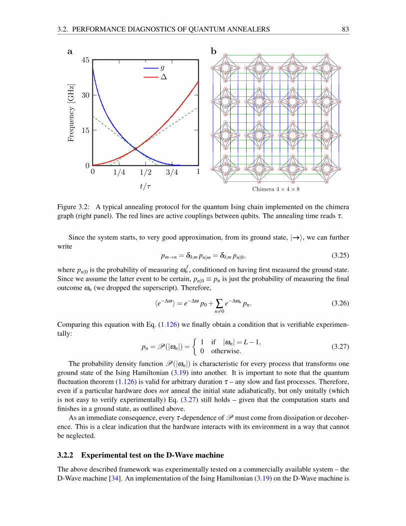
3.2. PERFORMANCE DIAGNOSTICS OF QUANTUM ANNEALERS 83
a b
0 1/4 1/2 3/4 10
15
30
45
t/τ
Fre
qu
ency
[GH
z]g
∆
Chimera 4× 4× 8
Figure 3.2: A typical annealing protocol for the quantum Ising chain implemented on the chimeragraph (right panel). The red lines are active couplings between qubits. The annealing time reads τ .
Since the system starts, to very good approximation, from its ground state, |→→→〉, we can furtherwrite
pm→n = δ0,m pn|m = δ0,m pn|0, (3.25)
where pn|0 is the probability of measuring ωf
n , conditioned on having first measured the ground state.Since we assume the latter event to be certain, pn|0 ≡ pn is just the probability of measuring the finaloutcome ωn (we dropped the superscript). Therefore,
〈e−∆ω〉= e−∆ω p0 + ∑n6=0
e−∆ωn pn. (3.26)
Comparing this equation with Eq. (1.126) we finally obtain a condition that is verifiable experimen-tally:
pn = P(|ωn|) =
1 if |ωn|= L−1,0 otherwise.
(3.27)
The probability density function P(|ωn|) is characteristic for every process that transforms oneground state of the Ising Hamiltonian (3.19) into another. It is important to note that the quantumfluctuation theorem (1.126) is valid for arbitrary duration τ – any slow and fast processes. Therefore,even if a particular hardware does not anneal the initial state adiabatically, but only unitally (whichis not easy to verify experimentally) Eq. (3.27) still holds – given that the computation starts andfinishes in a ground state, as outlined above.
As an immediate consequence, every τ-dependence of P must come from dissipation or decoher-ence. This is a clear indication that the hardware interacts with its environment in a way that cannotbe neglected.
3.2.2 Experimental test on the D-Wave machine
The above described framework was experimentally tested on a commercially available system – theD-Wave machine [34]. An implementation of the Ising Hamiltonian (3.19) on the D-Wave machine is
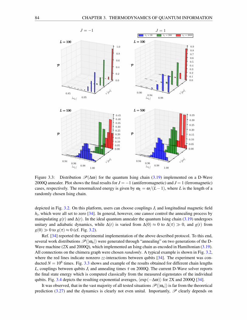
84 CHAPTER 3. THERMODYNAMICS OF QUANTUM INFORMATION
J = −1
|ωL |0.85
0.95
τ [µs]
0.0
0.2
0.4
0.6
0.8
1.0
P
L = 100
P
L = 100
P
L = 100
|ωL |
0.940.96
0.981.00
τ [µs]
0.00
0.05
0.10
0.15
0.20
0.25
0.30
0.35
0.40
0.45
P
L = 500
P
L = 500
P
L = 500
J = 1
|ωL |
0.900.94
0.98
τ [µs]
0.0
0.1
0.2
0.3
0.4
0.5
0.6
0.7
0.8
0.9
P
L = 100
P
L = 100
P
L = 100
ta = 20 ta = 200 ta = 2000
|ωL |
0.940.96
0.981.00
τ [µs]
0.00
0.05
0.10
0.15
0.20
0.25
0.30
0.35
P
L = 500
P
L = 500
P
L = 500
Figure 3.3: Distribution P(∆ω) for the quantum Ising chain (3.19) implemented on a D-Wave2000Q annealer. Plot shows the final results for J =−1 (antiferromagnetic) and J = 1 (ferromagnetic)cases, respectively. The renormalized energy is given by ωL = ω/(L−1), where L is the length of arandomly chosen Ising chain.
depicted in Fig. 3.2. On this platform, users can choose couplings Ji and longitudinal magnetic fieldhi, which were all set to zero [34]. In general, however, one cannot control the annealing process bymanipulating g(t) and ∆(t). In the ideal quantum annealer the quantum Ising chain (3.19) undergoesunitary and adiabatic dynamics, while ∆(t) is varied from ∆(0) ≈ 0 to ∆(τ) 0, and g(t) fromg(0) 0 to g(τ)≈ 0 (cf. Fig. 3.2).
Ref. [34] reported the experimental implementation of the above described protocol. To this end,several work distributions P(|ωn|) were generated through “annealing” on two generations of the D-Wave machine (2X and 2000Q), which implemented an Ising chain as encoded in Hamiltonian (3.19).All connections on the chimera graph were chosen randomly. A typical example is shown in Fig. 3.2,where the red lines indicate nonzero zz-interactions between qubits [34]. The experiment was con-ducted N = 106 times. Fig. 3.3 shows and example of the results obtained for different chain lengthsL, couplings between qubits Ji and annealing times τ on 2000Q. The current D-Wave solver reportsthe final state energy which is computed classically from the measured eigenstates of the individualqubits. Fig. 3.4 depicts the resulting exponential averages, 〈exp(−∆ω)〉 for 2X and 2000Q [34].
It was observed, that in the vast majority of all tested situations P(|ωn|) is far from the theoreticalprediction (3.27) and the dynamics is clearly not even unital. Importantly, P clearly depends on
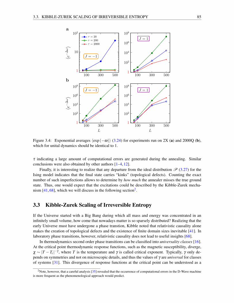
3.3. KIBBLE-ZUREK SCALING OF IRREVERSIBLE ENTROPY 85
J = −1
100 300 5001
10
102
〈e−∆ω〉
τ = 20
τ = 200
τ = 2000
a
J = 1
100 300 5001
102
104
106
108
J = −1
100 300 5001
102
104
106
108
L
〈e−∆ω〉
b
J = 1
100 300 5001
102
104
106
108
L
Figure 3.4: Exponential averages 〈exp(−ω)〉 (3.24) for experiments run on 2X (a) and 2000Q (b),which for unital dynamics should be identical to 1.
τ indicating a large amount of computational errors are generated during the annealing. Similarconclusions were also obtained by other authors [1–4, 12].
Finally, it is interesting to realize that any departure from the ideal distribution P (3.27) for theIsing model indicates that the final state carries “kinks” (topological defects). Counting the exactnumber of such imperfections allows to determine by how much the annealer misses the true groundstate. Thus, one would expect that the excitations could be described by the Kibble-Zurek mecha-nism [41, 68], which we will discuss in the following section2.
3.3 Kibble-Zurek Scaling of Irreversible Entropy
If the Universe started with a Big Bang during which all mass and energy was concentrated in aninfinitely small volume, how come that nowadays matter is so sparsely distributed? Realizing that theearly Universe must have undergone a phase transtion, Kibble noted that relativistic causality alonemakes the creation of topological defects and the existence of finite domain sizes inevitable [41]. Inlaboratory phase transitions, however, relativistic causality does not lead to useful insights [68].
In thermodynamics second order phase transitions can be classified into universality classes [16].At the critical point thermodynamic response functions, such as the magnetic susceptibility, diverge,χ ∼ |T −Tc|−γ , where T is the temperature and γ is called critical exponent. Typically, γ only de-pends on symmetries and not on microscopic details, and thus the values of γ are universal for classesof systems [31]. This divergence of response functions at the critical point can be understood as a
2Note, however, that a careful analysis [35] revealed that the occurrence of computational errors in the D-Wave machineis more frequent as the phenomenological approach would predict.
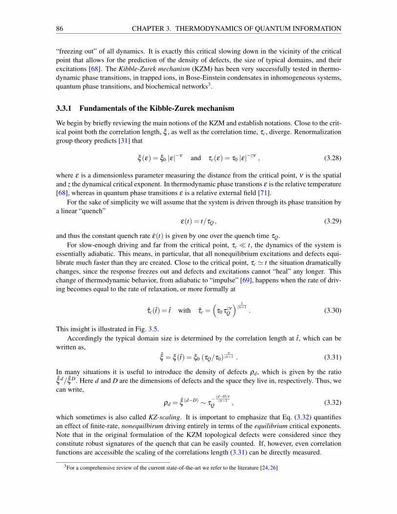
86 CHAPTER 3. THERMODYNAMICS OF QUANTUM INFORMATION
“freezing out” of all dynamics. It is exactly this critical slowing down in the vicinity of the criticalpoint that allows for the prediction of the density of defects, the size of typical domains, and theirexcitations [68]. The Kibble-Zurek mechanism (KZM) has been very successfully tested in thermo-dynamic phase transitions, in trapped ions, in Bose-Einstein condensates in inhomogeneous systems,quantum phase transitions, and biochemical networks3.
3.3.1 Fundamentals of the Kibble-Zurek mechanism
We begin by briefly reviewing the main notions of the KZM and establish notations. Close to the crit-ical point both the correlation length, ξ , as well as the correlation time, τc, diverge. Renormalizationgroup theory predicts [31] that
ξ (ε) = ξ0 |ε|−ν and τc(ε) = τ0 |ε|−zν , (3.28)
where ε is a dimensionless parameter measuring the distance from the critical point, ν is the spatialand z the dynamical critical exponent. In thermodynamic phase transtions ε is the relative temperature[68], whereas in quantum phase transitions ε is a relative external field [71].
For the sake of simplicity we will assume that the system is driven through its phase transition bya linear “quench”
ε(t) = t/τQ , (3.29)
and thus the constant quench rate ε(t) is given by one over the quench time τQ.For slow-enough driving and far from the critical point, τc t, the dynamics of the system is
essentially adiabatic. This means, in particular, that all nonequilibrium excitations and defects equi-librate much faster than they are created. Close to the critical point, τc ' t the situation dramaticallychanges, since the response freezes out and defects and excitations cannot “heal” any longer. Thischange of thermodynamic behavior, from adiabatic to “impulse” [69], happens when the rate of driv-ing becomes equal to the rate of relaxation, or more formally at
τc(t) = t with τc =(
τ0 τzν
Q
) 1zν+1
. (3.30)
This insight is illustrated in Fig. 3.5.Accordingly the typical domain size is determined by the correlation length at t, which can be
written as,ξ = ξ (t) = ξ0 (τQ/τ0)
ν
zν+1 . (3.31)
In many situations it is useful to introduce the density of defects ρd , which is given by the ratioξ d/ξ D. Here d and D are the dimensions of defects and the space they live in, respectively. Thus, wecan write,
ρd = ξ(d−D) ∼ τ
− (d−D)ν
zν+1Q , (3.32)
which sometimes is also called KZ-scaling. It is important to emphasize that Eq. (3.32) quantifiesan effect of finite-rate, nonequilbirum driving entirely in terms of the equilibrium critical exponents.Note that in the original formulation of the KZM topological defects were considered since theyconstitute robust signatures of the quench that can be easily counted. If, however, even correlationfunctions are accessible the scaling of the correlations length (3.31) can be directly measured.
3For a comprehensive review of the current state-of-the-art we refer to the literature [24, 26]
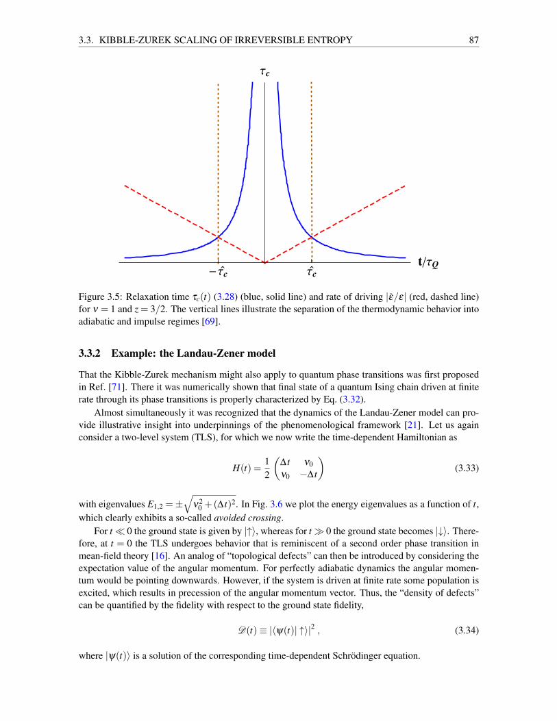
3.3. KIBBLE-ZUREK SCALING OF IRREVERSIBLE ENTROPY 87
τ
-τ /τ
τ
Figure 3.5: Relaxation time τc(t) (3.28) (blue, solid line) and rate of driving |ε/ε| (red, dashed line)for ν = 1 and z = 3/2. The vertical lines illustrate the separation of the thermodynamic behavior intoadiabatic and impulse regimes [69].
3.3.2 Example: the Landau-Zener model
That the Kibble-Zurek mechanism might also apply to quantum phase transitions was first proposedin Ref. [71]. There it was numerically shown that final state of a quantum Ising chain driven at finiterate through its phase transitions is properly characterized by Eq. (3.32).
Almost simultaneously it was recognized that the dynamics of the Landau-Zener model can pro-vide illustrative insight into underpinnings of the phenomenological framework [21]. Let us againconsider a two-level system (TLS), for which we now write the time-dependent Hamiltonian as
H(t) =12
(∆ t ν0ν0 −∆ t
)(3.33)
with eigenvalues E1,2 =±√
ν20 +(∆ t)2. In Fig. 3.6 we plot the energy eigenvalues as a function of t,
which clearly exhibits a so-called avoided crossing.For t 0 the ground state is given by |↑〉, whereas for t 0 the ground state becomes |↓〉. There-
fore, at t = 0 the TLS undergoes behavior that is reminiscent of a second order phase transition inmean-field theory [16]. An analog of “topological defects” can then be introduced by considering theexpectation value of the angular momentum. For perfectly adiabatic dynamics the angular momen-tum would be pointing downwards. However, if the system is driven at finite rate some population isexcited, which results in precession of the angular momentum vector. Thus, the “density of defects”can be quantified by the fidelity with respect to the ground state fidelity,
D(t)≡ |〈ψ(t)| ↑〉|2 , (3.34)
where |ψ(t)〉 is a solution of the corresponding time-dependent Schrodinger equation.
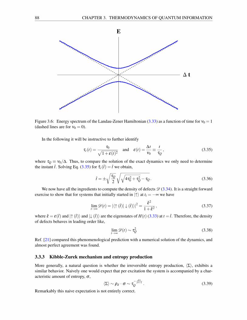
88 CHAPTER 3. THERMODYNAMICS OF QUANTUM INFORMATION
Δ
Figure 3.6: Energy spectrum of the Landau-Zener Hamiltonian (3.33) as a function of time for ν0 = 1(dashed lines are for ν0 = 0).
In the following it will be instructive to further identify
τc(t) =τ0√
1+ ε(t)2and ε(t) =
∆ tν0≡ t
τQ, (3.35)
where τQ ≡ ν0/∆. Thus, to compare the solution of the exact dynamics we only need to determinethe instant t. Solving Eq. (3.35) for τc(t) = t we obtain,
t =±√
τQ
2
√√4τ2
0 + τ2Q− τQ . (3.36)
We now have all the ingredients to compute the density of defects D (3.34). It is a straight forwardexercise to show that for systems that initially started in |↑〉 at ti =−∞ we have
limt→∞
D(t) = |〈↑ (t)| ↓ (t)〉|2 = ε2
1+ ε2 , (3.37)
where ε = ε(t) and |↑ (t)〉 and |↓ (t)〉 are the eigenstates of H(t) (3.33) at t = t. Therefore, the densityof defects behaves in leading order like,
limt→∞
D(t)∼ τ2Q (3.38)
Ref. [21] compared this phenomenological prediction with a numerical solution of the dynamics, andalmost perfect agreement was found.
3.3.3 Kibble-Zurek mechanism and entropy production
More generally, a natural question is whether the irreversible entropy production, 〈Σ〉, exhibits asimilar behavior. Naively one would expect that per excitation the system is accompanied by a char-acteristic amount of entropy, σ ,
〈Σ〉 ∼ ρd · σ ∼ τ− d ν
zν+1Q . (3.39)
Remarkably this naive expectation is not entirely correct.
3.3. KIBBLE-ZUREK SCALING OF IRREVERSIBLE ENTROPY 89
Maximum available work theorem. As we have discussed several times, the only processes thatcan be fully described by means of conventional thermodynamics are infinitely slow, equilibrium,a.k.a. quasistatic processes [16]. Nonequilibrium processes are characterized by the maximum avail-able work theorem [61]. Consider a general thermodynamic system which supplies work to a workreservoir, and which is in contact, but not in equilibrium with a heat reservoir, B. Then the first lawof thermodynamics can be written as,
∆E +∆EB = 〈W 〉 , (3.40)
where ∆E is the change of internal energy of the system, ∆EB is the energy exchanged with B, andas before 〈W 〉 denotes the average work. Accordingly the second law of thermodynamics states,
∆S+∆SB ≥ 0 , (3.41)
where ∆S is the change of thermodynamic entropy of the system, ∆SB is the change of entropyin B, and where we used that the entropy of the work reservoir is negligible [16]. Since the heatreservoir is so large that it is always in equilibrium at inverse temperature β we immediately canwrite β∆EB = ∆SB, and hence we always have
〈W 〉 ≥ ∆E−∆S/β ≡ ∆E . (3.42)
The thermodynamic quantity E is called exergy or availability [61], since it quantifies the maximalavailable work in any thermodynamic process.
KZ-scaling of the excess work. The maximal available work theorem [61] can be re-written interms of the excess work, 〈Wex〉, which is given by the total work, 〈W 〉, minus the quasistatic contri-bution, i.e., the availability ∆E ,
〈Wex〉= 〈W 〉−∆E . (3.43)
At constant temperature we can write ∆E ≡ 〈W 〉 − ∆E + ∆S/β [61], where ∆E is the change ofinternal energy in a quastistatic process, ∆S denotes the change of entropy, and β is the inversetemperature. For open equilibrium systems and isothermal processes the availability further reducesto the difference in Helmholtz free energy, ∆E = ∆F , why we can also write 〈Σ〉= β 〈Wex〉. However,more generally ∆E is the work performed during any quasistatic process, and thus 〈Wex〉 quantifies thenonequilibrium excitations arising from finite time driving – in isothermal as well as in more generalprocesses, and in open as well as in isolated systems.
Motivated by insights from finite-time thermodynamics [5] it has recently become clear that forsufficiently slow processes 〈Wex〉 can be expressed as quadratic form [13, 63],
〈Wex〉=∫
dtdλ
†
dtτc(t)I (t)
dλ
dt, (3.44)
where λ = (T,V,H, . . .) is the vector of all intensive parameters varied during the process, such astemperature T , volume V , magnetic field H, etc., and the integral is taken over the whole process.Furthermore, I (t) is the Fisher information matrix, which for a d dimensional system close to thecritical point and for only two intensive parameters such as T and H can be written as [50],
I (t)∼(|ε(t)|−α |ε(t)|b−1
|ε(t)|b−1 |ε(t)|−γ
)(3.45)
where γ = dν−2b, and α is the critical exponent corresponding to changes in temperature.
90 CHAPTER 3. THERMODYNAMICS OF QUANTUM INFORMATION
For the sake of simplicity we will now assume that only one intensive parameter, λ (t), is var-ied. Thus, we can express the (1×1)-dimensional Fisher information matrix in terms of the generalsusceptibility X (t),
I (t) = X (t) = X0 |ε(t)|−Λ (3.46)
where Λ is the critical exponent corresponding to the varied control parameter, e.g., for varied mag-netic fields we have Λ = γ , and for processes with time-dependent temperatures Λ = α .
The Kibble-Zurek hypothesis predicts that far from the critical point, |t| τc, the dynamics isessentially adiabatic, and hence 〈Wex〉 has non-vanishing contributions only in the impulse regime,|t| ≤ τc, cf. Fig. 3.5. Therefore, we can write,
〈Wex〉 ' λ2c
∫ nτc
−nτc
dt |ε(t)|2 τc(t)X (t) (3.47)
where λ (t) = λc(1− ε(t)) and n > 1 is a small, real constant 4. Employing Eqs. (3.28) and (3.46) itis then a simple exercise to show that
〈Wex〉=2λc X0 n−zν−Λ+1
zν +Λ−1τ
2−Λ
zν+10 τ
Λ−2zν+1
Q . (3.48)
Thus, we have shown that for systems that are driven at constant rate through a critical point theexcess work, 〈Wex〉, universally scales like [22],
〈Wex〉 ∼ τ
Λ−2zν+1
Q , (3.49)
which explicitly depends on the critical exponent Λ corresponding to how the system is driven. Thisbehavior is in full agreement with thermodynamics, since thermodynamic work is a process dependentquantity [16]. In other words, Eq. (3.49) expresses the fact that the excess work depends on how thesystem is driven through the critical point, whereas the typical domain size ξ (3.31) is independenton the choice of the intensive control parameter.
Quantum Ising model. Before we proceed we briefly comment on the consistency of our concep-tual arguments with an analytically solvable model. The Kibble-Zurek mechanism has been exten-sively studied for the quantum Ising chain (3.19). In the limit of infinitely many spins, N → ∞, andat ∆J = 1 the Ising has two critical points at gc =±1, with a ferromagnetic phase for |g|< 1 and twoparamagnetic phases for |g|> 1. The critical exponents are given by z = 1 and ν = 1.
A recent and very thorough study of the KZM in this model [32] revealed that the excess workscales like 〈Wex〉 ∼ τ
−1Q . In Ref. [32] this behavior was explained by noting that close to the critical
point the dispersion relation is no longer flat, but rather 〈Wex〉 ∼ ξ−2. This finding is fully consistentwith our general result (3.49). Note that Λ = 0 [39] and hence Eq. (3.49) immediately predicts〈Wex〉 ∼ τ
−1Q .
3.4 Error correction in adiabatic quantum computers
Not only for adiabatic quantum computers, but actually for any quantum computer it has been rec-ognized that the implementation of quantum error correcting algorithms [47] is a necessity. Looselyspeaking, any such algorithm works by encoding logical quantum states in several physical states
4We included the small, real constant n > 1 to guarantee that no non-negligible contributions to the excess work areneglected.
3.4. ERROR CORRECTION IN ADIABATIC QUANTUM COMPUTERS 91
that can be controlled separately and in parallel. In this way, the logical quantum states can be maderesilient against the effects of noise, such as decoherence and dissipation. However, due to the deli-cate nature of entanglement and decoherence, quantum error correction is a little more involved thancorrecting errors in classical computers.
Classical error correction. The basic principle is most easily demonstrated by a standard commu-nication problem. Imagine we wish to send one bit through a noisy classical channel. The effect ofthe noise can be described by a probability p, with which a bit flip occurs. Thus, with probability1− p the bit is transmitted correctly. Then, the bit can be protected by sending several independentcopies, and by “taking majority” votes at the receiving end. Suppose a logical bit is encoded in threephysical bits
0→ 000 and 1→ 111, (3.50)
and at the receiving end we obtain 010. Then with probability 1− (1− p)2 p the logical bit 0 wastransmitted, and only one physical bit was affected by the noise. It should be noted that such majorityvoting fails if two or more of the physical bits were flipped, which however is very unlikely as longas p is not too large.
This kind of code is known as repetition code, which closely resembles error correction in everyday conversations. To make sure to be understood, the same message is repeated several times.Unfortunately, generic features of quantum physics make error correction in quantum computers moreinvolved.
Quantum error correction. Naively, one would hope that quantum error correction could be facil-itated by similar principles. However, the intricacies of quantum information pose significant chal-lenges. These can be summarized under the following three issues [47]:
1. Measurement back action: Standard quantum measurements are rather invasive, and they typi-cally “destroy” the quantum state. Thus recovery of quantum information after observation isnot possible.
2. Continuous quantum noise: Quantum noise is not restricted to only discrete bit flips, but rathercontinuous and cumulative errors can occur affecting the phase, or resulting in loss of coherenceand entanglement.
3. Quantum states cannot be copied [65]: A hallmark result of quantum information theory isthe no cloning theorem [65]. Thus, it is not immediately clear how one would implement arepetition code.
Fortunately, none of these complications are debilitating enough to make quantum computing animpossibility. Rather, it has been shown that quantum bit flips as well as quantum phase flips canbe corrected. A seminal result is the Shor code [62] that protects a single qubit against any arbitraryerror. In this scheme,
|0〉 → (|000〉+ |111〉)3
2√
2and |1〉 → (|000〉− |111〉)3
2√
2. (3.51)
Rather remarkably, the utility of the Shor code has been demonstrated in several experiments, see forinstance Ref. [6, 15, 54].
However, most quantum error correcting codes have in common that they have been developed forgate based quantum computation. In this paradigm, a quantum algorithm is constructed as a sequenceof unitary maps acting upon a set of logical qubits.
92 CHAPTER 3. THERMODYNAMICS OF QUANTUM INFORMATION
3.4.1 Quantum error correction in quantum annealers
Naturally, any real quantum annealer will also be subject to effects of environmental noise, such asdecoherence and dissipation. However, in contrast to gate based quantum computers, for quantum an-nealers computational errors fall into two independent categories [67]: (i) fundamentally correctableerrors that are effects of environmental noise and (ii) fundamentally non-correctable errors that arisefrom excitations away from the ground state manifold due to finite time driving.
Fundamentally correctable errors – quantum annealing correction. For the first type of errorsa successful and experimentally tested error correction scheme was devised in Ref. [51]. To this end,consider the general Ising Hamiltonian
HIsing =N
∑i=1
hi σiz +
N
∑i< j
Ji j σizσ
jz , (3.52)
which allows to encode many hard and important optimization problems. Similarly to above, cf.Sec. 3.2, the solution of the optimization problem is found by letting the initial quantum state evolveunder the time-dependent Hamiltonian
H(t) = A(t)HX +B(t)HIsing for 0≤ t ≤ τ . (3.53)
Here, HX = ∑Ni=1 σ i
x, and A(t) and B(t) are time-dependent functions satisfying A(τ) = B(0) = 0.Quantum annealing correction is a combined strategy comprising an energy penalty (EP) together
with encoding and error correction. To this end, HIsing is “encoded” by replacing each σ iz by its
encoded counterpart⟨σ i
z⟩= ∑
n`=1 σ
i,`z and each σ i
zσj
z by⟨
σ izσ
jz
⟩= ∑
n`=1 σ
i,`z σ
j,`z , where ` is an index
counting the physical qubits encoding a single logical qubit. Therefore, the encoded Hamiltonian canbe written as ⟨
HIsing⟩=〈N〉∑i=1
hi⟨σ
iz⟩+〈N〉∑i< j
Ji j⟨σ
izσ
jz⟩
(3.54)
where 〈N〉 is the number of logical qubits. It is important to note that HX cannot be encoded in thissimple manner, as this would require n-body interactions.
Additional protection is provided by introducing a ferromagnetic penalty term
HP =−〈N〉∑i=1
n
∑`=1
σi,`z σ
iPz , (3.55)
which is a sum of stabilizer generators for the n+ 1 qubit repetition code. In effect, HP detects andenergetically penalizes all physical bit-flip errors, but not a bit-flip of the logical qubit.
Combining both encoding and energy penalty the total, encoded Hamiltonian becomes,
〈H(t)〉= A(t)HX +B(t)⟨HIsing(ν ,µ)
⟩, (3.56)
where⟨HIsing(ν ,µ)
⟩≡ ν
⟨HIsing
⟩+µ HP and ν is the “problem scale” and µ the penalty scale.
This quantum annealing correction was successfully tested for n = 3 on the second generationof the D-Wave machine [51, 52]. It was demonstrated that environmental noise can be efficientlycorrected for. However, such a quantum error correction code cannot circumvent fundamentally non-correctable errors.
3.4. ERROR CORRECTION IN ADIABATIC QUANTUM COMPUTERS 93
3.4.2 Adiabatic quantum computing – A case for shortcuts to adiabaticity
Finally, we will briefly outline a possible way of avoiding fundamentally non-correctable errors fromhappening in the first place. As we have already seen above, excitations that will naturally occurin non-equilibrium processes can be avoided by driving the systems sufficiently slowly. However,this requires a high-degree of control over the systems and still limits the utility of such devicesas the time scales required for their operation will tend to grow as the size of the system grows.Therefore, in recent years a great deal of theoretical and experimental research has been dedicated tomathematical tools and practical schemes to suppress these excitations in finite-time, nonequilibriumprocesses. To this end, a variety of techniques has been developed, such as the use of dynamicalinvariants, the inversion of scaling laws, the fast-forward technique, transitionless quantum driving,local counterdiabatic driving, optimal protocols from optimal control theory, optimal driving fromproperties of the quantum work statistics, “environment” assisted methods, using the properties ofLie algebras, and approximate methods such as linear response theory and fast quasistatic dynamics5.Among this plethora of different approaches, transitionless quantum driving stands out, since it is theonly method that suppresses excitations away from the adiabatic manifold at all instants.
Transitionless quantum driving. In the paradigm of transitionless quantum driving [10,27,28] oneconsiders a time-dependent Hamiltonian H0(t) with instantaneous eigenvalues εn(t) and eigenstates|n(t)〉. In the limit of infinitely slow variation of H0(t) a solution of the dynamics is given by
|ψn(t)〉= exp(− i
h
∫ t
0dsεn(s)−
∫ t
0ds〈n|∂sn〉
)|n(t)〉 . (3.57)
In this adiabatic limit no transitions between eigenstates occur [46], and each eigenstate acquiresa time-dependent phase that can be separated into a dynamical and a geometric contribution [9],represented by the two terms inside the exponential in the above expression.
Now, a corresponding Hamiltonian H(t) is constructed, such that the adiabatic approximationassociated with H0(t) (3.57) is an exact solution of the dynamics generated by H(t) under the time-dependent Schrodinger equation. Writing the time-evolution operator as U(t) = ∑n |ψn(t)〉〈n(0)|,one arrives at an explicit expression for H(t) [10, 27, 28]:
H = H0 +H1 = H0 + ih∑n(|∂tn〉〈n|− 〈n|∂tn〉 |n〉〈n|) . (3.58)
Here, the auxiliary Hamiltonian H1(t) enforces evolution along the adiabatic manifold of H0(t): ifa system is prepared in an eigenstate |n(0)〉 of H0(0) and subsequently evolves under H(t), thenthe term H1(t) effectively suppresses the non-adiabatic transitions out of |n(t)〉 that would arise inthe absence of this term. Through a little manipulation an equivalent expression for H1(t) can befound [10]
H1(t) = ih ∑m6=n
∑|m〉〈m|∂tH0|n〉〈n|
En−Em. (3.59)
From the set-up, transitionless quantum driving appears to be uniquely suited to suppress exci-tations from finite time driving and thereby bypass fundamentally non-correctable errors in quantumannealers.
5See Ref. [64] and references therein for an extensive review of these techniques.
94 CHAPTER 3. THERMODYNAMICS OF QUANTUM INFORMATION
3.4.3 Counterdiabatic Hamiltonian for scale-invariant driving
A major obstacle arises from the fact that it is rarely feasible to find closed-form expressions for thecounterdiabatic field (3.59), i.e., expressions that do not depend on the full spectral decomposition ofH0(t). However, there is a reasonably broad class of systems in which the situation greatly simplifies[23].
Example: Transitionless quantum driving of the harmonic oscillator. As a instructive exampleconsider the parametric harmonic oscillator
H0(t) =hω(t)
2
(a†a+
12
)(3.60)
where a† and a are the creation and annihilation operators, respectively. Using Eq. (3.59) we see thatin order to determine the auxiliary Hamiltonian we require the time derivative of the bare Hamiltonian.Using the definitions of a† and a in terms of position and momentum operators, x and p
a† =
√mω(t)
2h
(x− i
mω(t)p)
a =
√mω(t)
2h
(x+
imω(t)
p) (3.61)
it is evident that they are time-dependent operators. Taking the derivative of H0 we find
∂tH0 =hω
2
(a†a+
12
)+
hω
2(a†a+a†a
). (3.62)
where we have dropped the explicit time dependence for brevity and where ‘˙’ denotes the timederivative. From Eq. (3.61) we can readily determine the derivatives of the creation and annihiliationoperators
a† =ω
2ωa a =
ω
2ωa† (3.63)
Therefore we have the derivative of the bare Hamiltonian is given by
∂tH0 =hω
2
(a†a+
12
)+
hω
4
(a†2
+a2). (3.64)
To determine the auxiliary Hamiltonian we use Eq. (3.59). Since in the sums m 6= n, it is clear thatthe first term will not contribute. After some manipulation we finally arrive at the concise expression
H1(t) = ihω
4ω
(a2−a†2
). (3.65)
Notice that no assumptions or constraints have been put on the form of time-dependence. Thus, thetransitionless driving approach allows for an arbitrary ramp to be applied and for the driving to occur,at least in principle, in arbitrarily short times [18, 33].
General case. The parametric harmonic oscillator (3.60) belongs to the broader class of so-calledscale-invariantly driven systems. Scale-invariant driving refers to transformations of the Hamiltonianwhich can be absorbed by scaling of coordinates, time, energy, and possibly other variables to rewritethe transformed Hamiltonian in its original form up to a multiplicative factor. If only the potentialterm V (q,λ (t)) is modulated, its overall shape does not change under λ (0)→ λ (t).
3.4. ERROR CORRECTION IN ADIABATIC QUANTUM COMPUTERS 95
In the simplest case, consider a quantum system with a single degree of freedom,
H0(t) =p2
2m+V (q,λ (t)) =
p2
2m+
1γ2 V0
(q− f
γ
), (3.66)
where λ = (γ, f ) and V0(q) =V (q,λ (0)). Note that generally γ = γ(t) and f = f (t) are both allowedto be time-dependent, but we assume that they are independent of each other. This time-dependenceencompasses transport processes (γ(t) = 1), dilations (such as an expansion or compression, withf (t) = 0) and combined dynamics.
It can now be shown [23] that the auxiliary term H1(t) (3.58) can be brought into a form thatdoes not rely on the spectral decomposition of H0(t). To see this, consider that of ψ0
n (q) = 〈n|q〉 isan eigenfunction of the Hamiltonian H0(γ = 1, f = 0), then ψn(q,γ, f ) = α(γ)ψ0
n ((q− f )/γ) is aneigenfunction of H0(γ, f ), where α(γ) = 1/
√γ is a normalization constant.
Now, we want to use this symmetry to simplify H1(t) in Eq. (3.58). We can write,
H1(t) = ihλ ·∑m
(∣∣∣∇λm⟩〈m|−
⟨m|∇
λm⟩|m〉〈m|
), (3.67)
which reads in space representation
H1(t) = ihλ ·∑m
∫dq |q〉 ∇
λψm(q,λ ) 〈m|− ihλ ·∑
m
∫dq 〈m|q〉 ∇
λψm(q,λ ) |m〉〈m| . (3.68)
To simplify this expression, we note that
∇λ
ψn(q,λ ) =(
α ′(γ)α(γ)
ψn(q,γ)−q− f
γ∂qψn(q,γ), −∂qψn(q,γ)
). (3.69)
For the sake of clarity, let us treat both terms of H1(t) in (3.68) separately. We obtain for the first term
ihλ ·∑m
∫dq |q〉 ∇
λψm(q,λ ) 〈m|=
γ
γ(q− f ) p+ ihγ
α ′(γ)α(γ)
+ f p , (3.70)
while the second term reduces to
−ihλ ·∑m
∫dq 〈m|q〉 ∇
λψm(q,λ ) |m〉〈m|=−
ihγ
2γ− ihγ
α ′(γ)α(γ)
. (3.71)
Note that the second component of ∇λ
ψn(q,λ ) does not contribute, since the wavefunction vanishesat infinity due to normalizability. In conclusion, we obtain the explicit expression of the auxiliary CDHamiltonian,
H1(t) =γ
2γ[(q− f ) p+ p (q− f )]+ f p , (3.72)
where we used [q− f , p] = ih. Notice that H1(t) in Eq. (3.72) is of the general form H1 ∝ (qp+ pq)which is identical to (3.65).
Equation (3.72) is a remarkable result. For all driving protocols under which the original Hamil-tonian H0(t) is scale-invariant, i.e., where the time-dependent potential is of the form (3.66), theauxiliary term H1(t) takes the closed form (3.72). In particular, H1(t) is independent of the explicitenergy eigenfunctions, and only depends on the anticommutator, H1 ∝ q, p= qp+ pq, the generatorof dilations.
As a result, CD applies not only to single eigenstates, but also to non-stationary quantum superpo-sitions and mixed states. However, the expression (3.72) is still not particularly practical as non-localHamiltonians 6 are hard to realize in the laboratory.
6Hamiltonians that include products of space and momentum operator, q and p, are non-local, whereas local Hamilto-nians contain only terms that depend on at most sums of q and p.
96 CHAPTER 3. THERMODYNAMICS OF QUANTUM INFORMATION
Transitionless quantum driving and quantum annealing. We have seen above, cf. Sec. 3.2,that quantum spin chains, such as the Ising chain (3.19), offer a promising architecture for realizingquantum computational models. With this in mind, let us examine an alternative potential spin-system given by the ferromagnetic Lipkin-Meshkov-Glick (LMG) model, which allows us to exploitthe previous results for transitionless driving of the harmonic oscillator. The LMG model is describedby the Hamiltonian [17, 44, 55, 56].
H0(t) =−1N
(∑i< j
σix⊗σ
jx +χσ
iy⊗σ
jy
)−h(t)∑
iσ
iz (3.73)
where σx,y,z are again the Pauli spin-operators, h(t) is the time-dependent magnetic field strength, andχ is here the anisotropy parameter. By considering the collective spin operators S j = ∑i σ i
j/2 withj = x,y,z, the model can be written as
H0 =−2N
(S2
x +χS2y)−2hSz +
1+χ
2. (3.74)
For N→ ∞, the model can be solved through the Holstein-Primakoff (HP) transformation that allowsus to map the spin model to an equivalent harmonic oscillator. Similarly to the quantum Ising model,the LMG model exhibits a quantum phase transition in its ground state when h=1. Depending onthe phase that one is considering, the HP transformation must be taken along the direction that theclassical angular momentum,
S =N2(sinϕ cosφ ,sinϕ sinφ ,cosϕ), (3.75)
points. For h > 1 we find this is always along the z-axis. Neglecting terms higher than O(N) the HPtransformation in this limit is
S+ =√
Na, S− =√
Na†, Sz =N2−a†a, (3.76)
withSx =
12(S++S−) and Sy =
12i(S+−S−). (3.77)
This results in the mapped Hamiltonian in terms of bosonic creation and annihilation operators
Hb =−1−χ
2(a2 +a† 2)+(2h−1−χ)a†a−hN, (3.78)
which can then be written in diagonal form by performing the following Bogoliubov transformation
a = sinh(
α
2
)b† + cosh
(α
2
)b, (3.79)
a† = sinh(
α
2
)b+ cosh
(α
2
)b†, (3.80)
and taking
tanhα =1−χ
2h−1−χ, (3.81)
we finally obtain the harmonic oscillator equivalent for our Eq. (3.74)
Hho = 2√
(h−1)(h−χ)
(b†b+
12
)−h(N +1)+
1+χ
2. (3.82)
3.4. ERROR CORRECTION IN ADIABATIC QUANTUM COMPUTERS 97
For 0 < h < 1 this classical vector moves as the field, h, is varied. Therefore before performingthe HP transformation the Hamiltonian must be rotated to be inline with the direction of the classicalangular momentum, or equivalently, we must take the HP transformation along the direction thisvector points for a given value of h. We shall take the latter approach. For clarity, let us look at theslightly simpler case of χ = 0. In this case the classical vector moves between pointing along thex-axis (h = 0) and pointing along the z-axis (h = 1) according to ϕ = arccosh. Therefore, we take theHP transformation along this new direction
Hϕ =−(
2N
)(Sϕ
x )2−2hSϕ
z +1+χ
2,
Sϕx = Sx cosϕ−Sz sinϕ,
Sϕz = Sz cosϕ +Sx sinϕ.
(3.83)
We now use the same operators as in Eqs. (3.76) and (3.77) and therefore we have no need to per-form any inverse rotations after the mapping is complete. Doing this results in a different bosonicrepresentation,
Hb =−12
h2 (a2 +a† 2)+ (2−h2)a†a−(
h2N2
+h2+
N2
)+
12. (3.84)
Taking
tanhα =h2
2−h2 , (3.85)
in the Bogoliubov operators, we obtain the harmonic oscillator equivalent for χ = 0
Hho = 2√
(1−h2)
(b†b+
12
)− 1+h2
2N− 1
2. (3.86)
When considering arbitrary χ , the calculation is slightly more involved. However the final formachieved is
Hho = 2√
(1−h2)(1−χ)
(b†b+
12
)− 1+h2
2N− 1−χ
2. (3.87)
Using these mappings we can then use Eq. (3.65) to determine the corresponding auxiliary Hamil-tonian. For our purposes, working in units of h = 1, we take the effective frequency term appearingin Eqs. (3.82) and (3.87) as ω , i.e.
ω =
2√
(h−1)(h−χ), h > 1,2√(1−h2)(1−χ), 0 < h < 1,
(3.88)
recalling that h is time-dependent. Given that(
a2−a†2)=(
b2−b†2)
, and returning to the collectivespin operators, we find
H1 =
2h−1−χ
4N(h−1)(h−χ) (SxSy +SySx) , h > 1,2h(χ−1)
4N(1−h2)(1−χ)(SxSy +SySx) , 0 < h < 1.
(3.89)
Which are the exact correction terms required to achieve perfect finite-time adiabatic dynamics forN → ∞. What is immediately apparent is that the auxiliary Hamiltonian is not well-defined at thecritical point. Furthermore, examining Eqs. (3.89) we see that H1(t) contains complex and highlynon-local terms, meaning their experimental implementation is extremely challenging. A further
98 CHAPTER 3. THERMODYNAMICS OF QUANTUM INFORMATION
issue regarding the LMG model is that, while analytically exact in the thermodynamic limit, the cor-rection Hamiltonians do not recover exactly adiabatic dynamics when applied verbatim to finite Nsystems [17]. While we focused the analysis here on the harmonic oscillator and the LMG model,similar results can be achieved in the case of the quantum Ising model [25] by exploiting a concatena-tion of Landau-Zener models. Also in that case the corresponding auxiliary Hamiltonian was shownto be highly non-local.
Inadequacy of transitionless quantum driving for computing. Furthermore, despite its appealingset-up and potentially powerful applications, transitionless quantum driving is to date not very usefulfrom a computational point of view. With the exception of scale-invariant processes, to computethe auxiliary Hamiltonian the instantaneous eigenstates have to be known (3.58). Since in adiabaticquantum computation the outcome is encoded in the final ground state, one actually needs moreinformation to implement H1(t) (3.58) then is necessary to perform the computation exactly, i.e.,without any errors.
While this paints a somewhat bleak picture, we should realize that such analyses provide muchinformation regarding what must be done in order to achieve the requisite level of control. Clearly,critical spin systems are promising prototype platforms, but evidently for practical utility we willrequire alternative methods for coherently controlling them. Such a realization has led to an encour-aging line of research attempting to circumvent the most restrictive aspects of transitionless quantumdriving [17, 57].
Nevertheless further research has analyzed transitionless quantum driving in the context of uni-versal quantum computation [58] and gate teleportation [59]. Furthermore, transitionless quantumdriving stands as one of the most promising control techniques for coherently manipulating smallscale quantum systems, and in particular when applied to facilitating the adiabatic strokes of quan-tum heat cycles and even in enhancing metrological protocols [48]. Thus, we anticipate the comingyears to experience dedicated research efforts to adapt and generalize the framework of shortcuts toadiababiticty to develop novel tools and techniques tailored for quantum error correction.
3.5. CHECKLIST FOR “THERMODYNAMICS OF QUANTUM INFORMATION” 99
3.5 Checklist for “Thermodynamics of Quantum Information”
1. Information is physical and processing – writing as well as erasing – information “costs” ther-modynamic energy.
2. Purely quantum effects, such as coherence and entanglement can be utilized as additional ther-modynamic resources.
3. Quantum Stochastic Thermodynamics allows to assess the performance of quantum computers.
4. Quantum entropy production quantifies the amount of computational errors in quantum anneal-ers.
5. The Kibble-Zurek mechanism phenomenlogically predicts the occurrence of computational er-rors.
6. Quantum entropy production exhibits Kibble-Zurek scaling.
7. Quantum error correction is essential and schemes exist for any computational paradigm.
8. Shortcuts to adiabaticity suppress fundamentally non-correctable errors in quantum annealers.
3.6 Problems
Quantum thermodynamics of information 3.1
[1] An exactly soluble double-well potential is given by
V (x) =18
cosh(4x)−α cosh(2x)− 18,
where α > 1/2. Assume that the system was initially prepared in a corresponding Maxwell-Boltzmann distribution at temperature T , and that we seek to reset the system into right wellwith accuracy δ . To this end, assume that the final distribution is a narrow Gaussian centeredin the right well such that the probability to find the system in the left well is smaller than δ .For this situation, verify Landauer’s principle (3.3).
[2] Two qubits, A and B, are found in a quantum state, ρ , that is an even mixture of the Bell states
∣∣Φ±⟩= 1√2(|0〉A ⊗|0〉B±|1〉A ⊗|1〉B) and
∣∣Ψ±⟩= 1√2(|0〉A ⊗|1〉B±|1〉A ⊗|0〉B) .
Compute the amount of heat that is dissipated during a complete erasure of the stored quantuminformation, i.e., A and B are returned to
ρT = |0〉A ⊗|0〉B 〈0|A ⊗〈0|B .
How much of this heat is due to the erasure of classical information, and how much of this heatoriginates in destroying quantum correlations?
100 CHAPTER 3. THERMODYNAMICS OF QUANTUM INFORMATION
Performance diagnostics of quantum annealers 3.2
[3] The dynamics of a TLS weakly coupled to thermal noise is given by the Lindblad masterequation
dρ
dt=− i
h[H, ρ]+ γ (2σ−ρσ+−σ+σ−ρ−σ+ρσ−) ,
where H = −hω σz/2. Compute the quantum efficacy ε (1.127) for Ai = σx, A f = σx, andρ0 = exp(−βH)/Z.
[4] The strong coupling limit master equation with a σz system-bath operator reads,
dρ
dt=− i
h[H, ρ]+ γ ∑
i
(σ
izρσ
iz−ρ
),
where again H =−hω σz/2. Show that the dynamics under this master equation is unital.
Kibble-Zurek Scaling of Irreversible Entropy 3.3
[5] Consider a TLS described by the Landau-Zener Hamiltonian (3.33). Assuming that the systemwas initially prepared in state |↑〉 at ti =−t compute the quantum work distribution (1.102) forprocesses that end at t f = t. Show that the excess work exhibits Kibble-Zurek scaling.
[6] In mean-field theory the Landau free energy of a critical system is given by
E(m) =h2
8cosh(2m)−h cosh(m)− h2
8.
Identify the critical point and determine the critical exponents. Predict the behavior of theirreversible entropy production if the system is driven through the critical point at constant, butfinite rate.
Error correction in adiabatic quantum computers 3.4
[7] Consider two coupled qubits, which are described by the Ising Hamiltonian in transverse field
H(t) =−g(t)σ1x −g(t)σ
2x −∆(t)σ
1z σ
2z .
Compute the auxiliary Hamiltonian H1(t) (3.58) for transitionless quantum driving.
[8] Consider the encoded Hamiltonian 〈H(t)〉 in Eq. (3.56) for n = 2 and 〈N〉 = 3. Compute thecorresponding auxiliary Hamiltonian H1(t) (3.58) that would suppress finite-time excitationsin quantum annealing correction. Would it be possible to implement the total HamiltonianHtot(t) = 〈H(t)〉+H1(t) on a quantum annealer such as the D-Wave machine?
References
[1] T. Albash, S. Boixo, D. A. Lidar, and P. Zanardi. Quantum adiabatic markovian master equa-tions. New J. Phys., 14:123016, 2012.
[2] T. Albash, I. Hen, F. M. Spedalieri, and D. A. Lidar. Reexamination of the evidence for entan-glement in a quantum annealer. Phys. Rev. A, 92:062328, 2015.
[3] T. Albash and D. A. Lidar. Decoherence in adiabatic quantum computation. Phys. Rev. A,91:062320, 2015.
[4] T. Albash, D. A. Lidar, M. Marvian, and P. Zanardi. Fluctuation theorems for quantum pro-cesses. Phys. Rev. E, 88:032146, 2013.
[5] B. Andresen, P. Salamon, and R. S. Berry. Thermodynamics in finite time. Phys. Today, 37:62,1984.
[6] B. A. Bell, D. A. Herrera-Martı, M. S. Tame, D. Markham, W. J. Wadsworth, and J. G. Rarity.Experimental demonstration of a graph state quantum error-correction code. Nat. Commun.,5:3658, 2014.
[7] C. H. Bennett. The thermodynamics of computation—a review. Int. J. Theo. Phys., 21:905,1982.
[8] C. H. Bennett. Notes on Landauer’s principle, reversible computation, and Maxwell’s Demon.Stud. Hist. Philos. Sci. A, 34:501, 2003.
[9] M. V. Berry. Quantal phase factors accompanying adiabatic changes. Proc. R. Soc. A, 392:45,1984.
[10] M. V. Berry. Transitionless quantum driving. J. Phys. A: Math. Theor., 42:365303, 2009.
[11] A. Berut, A. Arakelyan, A. Petrosyan, S. Ciliberto, R. Dillenschneider, and E. Lutz. Experi-mental verification of Landauer’s principle linking information and thermodynamics. Nature,483:187, 2012.
[12] S. Boixo, T. Albash, F. M. Spedalieri, N. Chancellor, and D. A Lidar. Experimental signature ofprogrammable quantum annealing. Nat. Comm., 4:2067, 2013.
[13] M. V. S. Bonanca and S. Deffner. Optimal driving of isothermal processes close to equilibrium.J. Chem. Phys., 140:244119, 2014.
[14] H.-P Breuer and F. Petruccione. The theory of open quantum systems. Oxford, 2002.
[15] H.-J. Briegel, T. Calarco, D. Jaksch, J. I. Cirac, and P. Zoller. Quantum computing with neutralatoms. J. Mod. Opt., 47:415, 2000.
101
102 REFERENCES
[16] H. Callen. Thermodynamics and an Introduction to Thermostastistics. Wiley, New York, USA,1985.
[17] S. Campbell, G. De Chiara, M. Paternostro, G. M. Palma, and R. Fazio. Shortcut to Adiabaticityin the Lipkin-Meshkov-Glick Model. Phys. Rev. Lett., 114:177206, 2015.
[18] S. Campbell and S. Deffner. Trade-off between speed and cost in shortcuts to adiabaticity. Phys.Rev. Lett., 118:100601, 2017.
[19] S. Campbell, G. Guarnieri, M. Paternostro, and B. Vacchini. Nonequilibrium quantum boundsto Landauer’s principle: Tightness and effectiveness. Phys. Rev. A, 96:042109, 2017.
[20] A. Chenu, M. Beau, J. Cao, and A. del Campo. Quantum simulation of generic many-body opensystem dynamics using classical noise. Phys. Rev. Lett., 118:140403, 2017.
[21] B. Damski. The Simplest Quantum Model Supporting the Kibble-Zurek Mechanism of Topo-logical Defect Production: Landau-Zener Transitions from a New Perspective. Phys. Rev. Lett.,95:035701, 2005.
[22] S. Deffner. Kibble-zurek scaling of the irreversible entropy production. Phys. Rev. E, 96:052125,2017.
[23] S. Deffner, C. Jarzynski, and A. del Campo. Classical and quantum shortcuts to adiabaticity forscale-invariant driving. Phys. Rev. X, 4:021013, 2014.
[24] A. del Campo, T. W. B. Kibble, and W. H. Zurek. Causality and non-equilibrium second-orderphase transitions in inhomogeneous systems. J. Phys. Condens. Matter, 25:404210, 2013.
[25] A. del Campo, M. M. Rams, and W. H. Zurek. Assisted finite-rate adiabatic passage acrossa quantum critical point: Exact solution for the quantum Ising model. Phys. Rev. Lett.,109:115703, 2012.
[26] A. del Campo and W. H. Zurek. Universality of phase transition dynamics: Topological defectsfrom symmetry breaking. Int. J. Mod. Phys. A, 29:1430018, 2014.
[27] M. Demirplak and S. A. Rice. Adiabatic population transfer with control fields. J. Chem. Phys.A, 107:9937, 2003.
[28] M. Demirplak and S. A Rice. Assisted adiabatic passage revisited. J. Phys. Chem. B, 109:6838,2005.
[29] M. Esposito, K. Lindenberg, and C. Van den Broeck. Entropy production as correlation betweensystem and reservoir. New J. Phys., 12:013013, 2010.
[30] E. Farhi, J. Goldstone, S. Gutmann, and M. Sipser. Quantum Computation by Adiabatic Evolu-tion. arXiv:quant-ph/0001106, 2000.
[31] M. E. Fisher. The renormalization group theory of critical behavior. Rev. Mod. Phys., 46:597,1974.
[32] A. Francuz, J. Dziarmaga, B. Gardas, and W. H. Zurek. Space and time renormalization in phasetransition dynamics. Phys. Rev. B, 93:075134, 2016.
REFERENCES 103
[33] K. Funo, J.-N. Zhang, C. Chatou, K. Kim, M. Ueda, and A. del Campo. Universal work fluctu-ations during shortcuts to adiabaticity by counterdiabatic driving. Phys. Rev. Lett., 118:100602,2017.
[34] B. Gardas and S. Deffner. Quantum fluctuation theorem for error diagnostics in quantum an-nealers. Sci. Rep., 8:17191, 2018.
[35] B. Gardas, J. Dziarmaga, W. H. Zurek, and M. Zwolak. Defects in quantum computers. Sci.Rep., 8:4539, 2018.
[36] J. Goold, M. Paternostro, and K. Modi. Nonequilibrium quantum Landauer principle. Phys.Rev. Lett., 114:060602, 2015.
[37] G. Guarnieri, S. Campbell, J. Goold, S. Pigeon, B. Vacchini, and M. Paternostro. Full countingstatistics approach to the quantum non-equilibrium Landauer bound. New J. Phys., 19:103038,2017.
[38] M. B. Hastings. Quantum adiabatic computation with a constant gap is not useful in one dimen-sion. Phys. Rev. Lett., 103:050502, 2009.
[39] I. Herbut. A modern approach to critical phenomena. Cambridge University Press, Cambridge,2007.
[40] T. Kadowaki and H. Nishimori. Quantum annealing in the transverse Ising model. Phys. Rev. E,58:5355, 1998.
[41] T. W. B. Kibble. Topology of cosmic domains and strings. J. Phys. A: Math. Gen, 9:1387, 1976.
[42] R. Landauer. Irreversibility and heat generation in the computing process. IBM. J. Res. Dev.,5:183, 1961.
[43] T. Lanting, A. J. Przybysz, A. Yu. Smirnov, F. M. Spedalieri, M. H. Amin, A. J. Berkley, R. Har-ris, F. Altomare, S. Boixo, P. Bunyk, N. Dickson, C. Enderud, J. P. Hilton, E. Hoskinson, M. W.Johnson, E. Ladizinsky, N. Ladizinsky, R. Neufeld, T. Oh, I. Perminov, C. Rich, M. C. Thom,E. Tolkacheva, S. Uchaikin, A. B. Wilson, and G. Rose. Entanglement in a quantum annealingprocessor. Phys. Rev. X, 4:021041, 2014.
[44] H. J. Lipkin, N. Meshkov, and A. J. Glick. Validity of many-body approximation methods for asolvable model: (i). exact solutions and perturbation theory. Nucl. Phys., 62:188, 1965.
[45] K. Maruyama, F. Nori, and V. Vedral. Colloquium: The physics of maxwell’s demon andinformation. Rev. Mod. Phys., 81:1–23, 2009.
[46] A. Messiah. Quantum Mechanics, volume II. John Wiley & Sons, Amsterdam, The Netherlands,1966.
[47] M. A. Nielsen and I. L. Chuang. Quantum Computation and Quantum Information. CambridgeUniversity Press, Cambridge, UK, 2010.
[48] S. Pang and A. N. Jordan. Optimal adaptive control for quantum metrology with time-dependentHamiltonians. Nat. Commun., 8:14695, 2017.
[49] J. M. R. Parrondo, J. M. Horowitz, and T. Sagawa. Thermodynamics of information. NaturePhys., 11:131, 2015.
104 REFERENCES
[50] M. Prokopenko, J. T. Lizier, O. Obst, and X. R. Wang. Relating Fisher information to orderparameters. Phys. Rev. E, 84:041116, 2011.
[51] K. L. Pudenz, T. Albash, and D. A. Lidar. Error-corrected quantum annealing with hundreds ofqubits. Nat. Comm., 5:3243, 2014.
[52] K. L. Pudenz, T. Albash, and D. A. Lidar. Quantum annealing correction for random Isingproblems. Phys. Rev. A, 91:042302, 2015.
[53] D. Reeb and M. M. Wolf. An improved Landauer principle with finite-size corrections. New J.Phys., 16:103011, 2014.
[54] M. D. Reed, L. DiCarlo, S. E. Nigg, L. Sun, L. Frunzio, S. M. Girvin, and R. J. Schoelkopf. Real-ization of three-qubit quantum error correction with superconducting circuits. Nature, 482:382,2012.
[55] P. Ribeiro, J. Vidal, and R. Mosseri. Thermodynamical limit of the Lipkin-Meshkov-Glickmodel. Phys. Rev. Lett., 99:050402, 2007.
[56] P. Ribeiro, J. Vidal, and R. Mosseri. Exact spectrum of the Lipkin-Meshkov-Glick model in thethermodynamic limit and finite-size corrections. Phys. Rev. E, 78:021106, 2008.
[57] H. Saberi, T. Opatrny, K. Mølmer, and A. del Campo. Adiabatic tracking of quantum many-body dynamics. Phys. Rev. A, 90:060301, 2014.
[58] A. C. Santos and M. S. Sarandy. Superadiabatic controlled evolutions and universal quantumcomputation. Sci. Rep., 5:15775, 2015.
[59] A. C. Santos, R. D. Silva, and M. S. Sarandy. Shortcut to adiabatic gate teleportation. Phys.Rev. A, 93:012311, 2016.
[60] N. Savage. Quantum computers compete for supremacy. Scientific American, July, 2017.
[61] F. Schlogl. Probability and Heat. Springer, Wiesbaden, Germany, 1989.
[62] P. W. Shor. Scheme for reducing decoherence in quantum computer memory. Phys. Rev. A,52:R2493, 1995.
[63] D. A. Sivak and G. E. Crooks. Thermodynamic Metrics and Optimal Paths. Phys. Rev. Lett.,108:190602, 2012.
[64] E. Torrontegui, S. Ibanez, S. Martınez-Garaot, M. Modugno, A. del Campo, D. Guery-Odelin,A. Ruschhaupt, X. Chen, and J. G. Muga. Shortcuts to Adiabaticity. Adv. At. Mol. Opt. Phys.,62:117, 2013.
[65] W. K. Wootters and W. H. Zurek. A single quantum cannot be cloned. Nature, 299:802, 1982.
[66] K. C. Young, R. Blume-Kohout, and D. A. Lidar. Adiabatic quantum optimization with thewrong hamiltonian. Phys. Rev. A, 88:062314, 2013.
[67] K. C. Young, M. Sarovar, and R. Blume-Kohout. Error suppression and error correction inadiabatic quantum computation: Techniques and challenges. Phys. Rev. X, 3:041013, 2013.
[68] W. H. Zurek. Cosmological experiments in superfluid helium? Nature, 317:505, 1985.
REFERENCES 105
[69] W. H. Zurek. Cosmological experiments in condensed matter systems. Phys. Rep., 276:177,1996.
[70] W. H. Zurek. Decoherence, einselection, and the quantum origins of the classical. Rev. Mod.Phys., 75:715, 2003.
[71] W. H. Zurek, U. Dorner, and P. Zoller. Dynamics of a Quantum Phase Transition. Phys. Rev.Lett., 95:105701, 2005.
Epilogue
In this book we have attempted to, concisely, explore several facets of modern thermodynamics –from its axiomatic origins through to the development of Stochastic Thermodynamics and right up tothe most recent advances in its quantum formulation. Indeed, as a physical theory thermodynamicsis imposing in both its range of applicability and the deep insights into the workings of the universeit provides. For instance, as we have seen in Chapter 1, the role of entanglement in providing aunique means of deriving canonical concepts in statistical mechanics enhances the special place thatthe seemingly counterintuitive notions of quantum mechanics play in dictating how the world aroundus emerges. Naturally, we have seen that a consistent quantum formulation of the core tenants of ther-modynamics – quantum work and heat – is a delicate issue. Nevertheless, as established throughoutChapters 2 and 3, as technological progress marches (and miniaturizes) on understanding the thermo-dynamics in this regime is crucial. It is therefore our hope that the material in this book has providedthe necessary tools to handle the exciting challenges ahead.
Of course there is a whole host of interesting topics that we simply could not cover in the limitedspace available, one particular field being so-called resource theories. As the field of quantum in-formation reached maturity, a greater focus was given to understanding the manipulation of quantumsystems from a resource theoretic viewpoint. Indeed, it is clear that quantum features, in particularentanglement and other quantum correlations, are quantifiable resources for information processingand other tasks. Such an approach is fruitful when applied to understanding Quantum Thermodynam-ics. The resource theory of Quantum Thermodynamics has shed light into what constitutes thermallyfree states and operations, thus providing insight into the thermodynamic cost of quantum informa-tion. Other exciting work has gone into exploring thermodynamic principles in cold atomic systems,where theoretical and experimental tools in this arena are progressing in tandem, and quantum biol-ogy, which studies the impact of genuine quantum effects on biological processes.
We close with some aspirations for the future. As new quantum technologies develop the un-derstanding of their thermodynamic working principles is key to ensuring practical, energy efficientdevices. The topics covered in Chapter 3 gave a snap-shot of some of the more recent developmentsin this regard, however as mentioned, a great deal of work still needs done before the full promise ofquantum technologies can be realized. Nevertheless, the great pace at which the young communitycontinues to drive the field leaves us with no doubt that, as with the incredible advances that classicalthermodynamics provided little over a century and a half ago, Quantum Thermodynamics has manymore remarkable insights yet to come.
If one cannot enjoy reading a book over and over again, there is no use in reading it at all.(Oscar Wilde)
106
Acknowledgments
Sebastian Deffner.– Every academic strives to live up to his mentors. In my case, this is an almostinconceivable challenge, since I have been very fortunate to have learned from the best. In particular,I would like to thank my Doktorvater and friend Eric Lutz for making me his first student. Withouthis vision and foresight I would never have started to work in Quantum Thermodynamics. I will alsoforever be indebted to Chris Jarzynski for putting up with me during my early postdoctoral phase.His kindness and unwavering support paired with his unmatched understanding of Thermodynamicsallowed me to grow into the physicist I am today. Finally, I will never forget the lessons I wastaught by Wojciech H. Zurek. Being one of the most influential theoretical physicists he openedmy eyes to the insurmountable variety of questions that can be addressed with the tools of QuantumThermodynamics. His dedication to and his joy in unlocking the mysteries of the Universe, while atthe same time remaining grounded in what really counts in life, remind me almost every day why Ibecame a theoretical physicist and what kind of man I want to be.
I would also like to thank my dear friends and collaborators, who helped me hone my thinkingand whose work contributed to this book. In particular, I am grateful to Marcus Bonanca, BartłomeijGardas, Frederico Brito, Haitao Quan, and Obinna Abah. I am looking forward to all the excitingresearch we will be tackling in the years to come.
Finally, I would like to thank my family, my parents, Alfred and Isabella, and my brother,Christoph, for accepting me for who I am and reminding me to never give up on my dreams. Last butnot least, I am lacking words to express the importance of my partner in crime, my closest confidante,and mother of my children, Catherine. Thank you for always reminding me to keep fighting, formaking me a better man, and for never giving up on me.
Maximillian and Alexander, like everything I do, this is for you!
Steve Campbell.– I have been fortunate to have enjoyed a menagerie of collaborators over my rela-tively short research career so far. They all, in their own way, have contributed to how my interestshave developed over the years which ultimately led to this work, and for this I am forever grateful. Iam particularly indebted to those friends whose work formed the basis for some parts of this book:Marco Genoni, Gian Luca Giorgi, John Goold, Giacomo Guarnieri, Simon Pigeon, Maria Popovic,and Bassano Vacchini. I am also eternally grateful to Tony Apollaro, Barıs Cakmak, Gabriele DeChiara, Mossy Fogarty, and Massimo Palma for the many years of stimulating discussions, punctu-ated with great refreshments, may they long continue.
I am lucky to have gained much of my scientific training from two world-leading physicists,Mauro Paternostro and Thomas Busch. The lessons learned from their expert guidance is woventhroughout this book. I feel privileged to have benefitted from their friendship for so many years.
My parents, Larry and Shirley, and brother, Jaymz, I am thankful for all they continue to do forme. Finally, to my loves Flora and Qubit (the cat). Your support and encouragement to undertake andcomplete this book is the only reason I made it through. For putting up with the life of an early careeracademic trying to find his place, I owe you everything.
107


