Comprehensive Summaries of Uppsala Dissertations from the Faculty of Science and Technology 217

Quark and Lepton Interactions

Studies of Quantum Chromo Dynamics and Majorana Neutrinos

BY

JOHAN RATHSMAN

ACTA UNIVERSITATIS UPSALIENSIS UPPSALA 1996

Dissertation for the Degree of Doctor of Philosophy in high energy physics pre· sented at Uppsala University in 1996

ABSTRACT

Rathsman, J. 1996. Quark and Lepton Interactions: Studies of Quantum Chroml Dynamics and Majorana Neutrinos. Acta Universitatis Upsaliensis. Compre· hensive Summaries of Uppsala Dissertations from the Faculty of Science anc Technology 217. 53 pp. Uppsala. ISBN 91-554-3786-9.

Heavy Majorana neutrinos, predicted in various extensions of the Standarc Model, can explain the small masses of the light neutrinos through the see­saw mechanism. The production of heavy Majorana neutrinos in ep collisiom through mixing is investigated and effective search strategies are developed. F01 a mixing of 1% and an integrated luminosity of 1 fb- 1 , the discovery limits an found to be '" 160 GeV at HERA and", 700 GeV at LEPEBLHC.

The deep inelastic scattering experiments at the HERA electron-proton col­lider (..jS ~ 300 Ge V) provide new tests of QCD dynamics at small-x. A unified description is presented which gives reasonably good agreement with availabl~ data, both on transverse energy flows and rapidity gap events in form of th~ diffractive structure function. The description is based on first order QCD rna· trix elements and leading-log Q2 parton showers together with non-perturbativ( soft colour interactions and string hadronisation. The inclusion of coherenc( effects in parton showers in different Monte Carlo programs is studied both a1 parton and hadron level.

The theoretical uncertainty due to the renormalisation scheme ambiguity if investigated for the next-to-leading order deep inelastic scattering 2+1 jet cross· section. The uncertainties limit the range of jet cut-offs that can be used.

The conformal limit arguments fix the renormalisation scheme when tw< observables are related by requil;ing all effects of scale breaking ({3 =f. 0) t( be absorbed into the running of the strong coupling as. It is shown how the conformal limit arguments can be extended to next-to-next-to-leading order tc fix both the renormalisation scale and {32, giving a commensurate {32 relation.

Johan Rathsman, Department of Radiation Sciences, Uppsala University, Bo: 535, S-75121 Uppsala, Sweden.

© Johan Rathsman 1996

ISSN 1104-232X ISBN 91-554-3786-9

Printed in Sweden by Fyris Tryck, Uppsala, 1996

To my family

Was sich iiberhaupt sagen liiBt, liiBt sich klar sagen;

und wovon man nicht reden kann, dariiber muB man schweigen.

Ludwig Wittgenstein

This thesis is based on the following papers, which will be referred to in the text by their Roman numerals:

I G. Ingelman and J. Rathsman, Heavy Majorana Neutrinos at ep colliders, Zeitschrift fUr Physik C 60 (1993) 243.

II G. Ingelman and J. Rathsman, Parton Cascade Models and QCD coherence at HERA, Journal of Physics G: Nuclear and Particle Physics, 19 (1993) 1594.

III A. Edin, G. Ingelman and J. Rathsman, Soft Colour Interactions as the Origin of Rapidity Gaps in DIS, Physics Letters B 366 (1996) 371.

IV A. Edin, G. Ingelman and J. Rathsman, Unified Description of Rapidity Gaps and Energy Flows in DIS Final States, DESY 96-060 (1996) submit­ted to Zeitschrift fUr Physik C.

V G. Ingelman and J. Rathsman, Renormalisation Scale Uncertainty in the DIS 2+1 jet Cross-Section, Zeitschrift fUr Physik C 63 (1994) 589.

VI J. Rathsman, Fixing the Renormalisation Scheme in NNLO Perturbative QCD Using Conformal Limit Arguments, TSL/ISV-96-0130 (1996) sub­mitted to Physical Review D.

VII J. Rathsman and G. Ingelman, MAJOR 1.5 - A Monte Carlo Genera­tor for Heavy Majorana Neutrinos in ep Collisions, DESY 96-059 (1996) submitted to Computer Physics Communications.

VIII G. Ingelman, J. Rathsman and G. A. Schuler, AROMA 2.2 - A Monte Carlo Generator for Heavy Flavour Events in ep Collisions, DESY 96-058 (1996) submitted to Computer Physics Communications.

IX G. Ingelman, A. Edin and J. Rathsman, LEPTO 6.5 - A Monte Carlo Gen­erator for Deep Inelastic Lepton-Nucleon Scattering, DESY 96-057 (1996) submitted to Computer Physics Communications.

Content's

1 Introduction 1 1.1 Historical background 1 1.2 Deep inelastic scattering . . 6 1.3 Testing the Standard Model 7

2 Theoretical framework of particle physics 11 2.1 Introduction ........ . 11

2.1.1 The Gauge principle 11 2.1.2 Perturbation theory 13

2.2 Electroweak theory . . . . . 16 2.2.1 The electroweak Standard Model 16 2.2.2 Extended electroweak theories 18

2.3 Quantum Chromo Dynamics ..... . 20 2.3.1 Asymptotic freedom . . . . . . . 20 2.3.2 Deep inelastic electron proton scattering. 22 2.3.3 Hadronic final states ........... . 25

3 Phenomenological models 27 3.1 Monte Carlo event generators 27

4 Summary of papers 31 4.1 Search for heavy Majorana neutrinos 31

4.1.1 Paper I ........... 31 4.2 Strong interaction phenomenology 32

4.2.1 Paper II . 32 4.2.2 Paper III · ......... 33 4.2.3 Paper IV · ......... 34

4.3 Renormalisation scheme ambiguity 35 4.3.1 Paper V .... 35 4.3.2 Paper VI · .... 35

4.4 Monte Carlo programs . . 36 4.4.1 Paper VII: MAJOR 36 4.4.2 Paper VIII: AROMA 37 4.4.3 Paper IX: LEPTO . . 37

v

vi Contents

5 Conclusions and outlook 39

Acknowledgements 41

Bibliography 43

Chapter 1

Introduction

1.1 Historical background

The quest for understanding the fundamental structure of matter started already with the ancient Greek philosophers. Around 600 BC Thales from Miletos sup­posedly said that 'everything consists of water'. Later Anaximenes of the same school claimed that everything consists of air of different density and accord­ing to Herakleitos fire was the fundamental constituent. The long-lived belief that water, air, fire and earth were the fundamental constituents started with Empedokles from Akragas in the 5th century BC and dominated physics and chemistry until the 17th century. Empedokles also had two active principles, love and discord which unite and divide the four elements respectively. These two principles were also thought of as elements giving in total six elements.

The concept of atoms was introduced by Leukippos and later developed by Demokritos (420 BC). The atoms had the following properties; rigidity, solidity and indivisibility, the latter meaning that it could not be physically broken into pieces. In addition they were thought to be so small that they could not be observed and they existed in the empty space. Changes in a material were thought of as a redistribution of the atoms and could thereby be explained but the atoms themselves could not be explained'.

The general concept today of how the world is constituted has not changed much since then. Still the concept of fundamental building blocks is used and between these building blocks there are different forces which are attractive or repulsive. Unfortunately the term atom is today used for what at the time of their discovery was thought to be fundamental elements but later showed to be composite objects. In the modern version of the term, an atom consists of a nucleus surrounded by a cloud of electrons. The nucleus has positive electric charge and the electrons have negative giving a total electric charge of zero for the atom.

The electrons where first observed by J. J. Thomson [Th097] and in 1911 Rutherford found that the atoms have a nucleus. Two of Rutherford's assistants, Geiger and Marsden, irradiated a thin gold foil with a-particles (helium nuclei) from a radioactive source and observed how they were scattered or deflected when

1

2 Chapter 1 Introduction

they passed through the foil. Most of the a-particles were scattered at small angles but some of them were scattered at large angles. From the measured amount of scattered a-particles at different angles, Rutherford could deduce that atoms have a nucleus in the center where the mass and positive charge is concentrated.

The nucleus is about 10 000 times smaller than the atom and it consists of protons which have positive electric charge, discovered by Rutherford [Rhul1, Rhu19], and neutrons which are electrically neutral and were discovered much later by Chadwick [Cha32]. With these three constituent particles, the electron, proton and neutron, one could build all atoms and understand the periodic table. What at first had seemed to be almost one hundred different atoms could now be understood using just three building blocks and their electromagnetic and nuclear interactions.

In addition to the electron, proton and neutron one more particle, the photon (T) was known. In the end of the 1880's Hertz had showed that light is an electromagnetic wave which can be described by Maxwell's equations and in 1905 Einstein [Ein05] suggested that light also has a particle nature, Le. it consists of photons. This particle-wave duality later became one of the corner stones of quantum mechanics.

The photon mediates the electromagnetic force, Le. when two particles in­teract electromagnetically with each other they exchange photons. The elec­tromagnetic force acts on particles with electric charge like the electron and the proton, and it binds the electrons to the nucleus in the atom. The force is attrac­tive between charges of opposite sign and repulsive between charges of the same sign and thus it cannot be responsible for keeping the nucleus together. Since the positively charged protons are repelled by each other electromagnetically, there must exist a stronger nuclear force which binds the protons and neutrons together.

Generally, particles can be divided into two groups, matter particles like the electron, proton and neutron which are called fermions and force carriers like the photon which are called bosons. The difference between fermions and bosons is quantum mechanical. Fermions obey Pauli's exclusion principle [Pau40] ac­cording to which there can only be one fermion in a given quantum mechanical state. For bosons there is no limitation of the number of particles in a given state. In a laser beam for example, all photons are in the same state which gives an extremely bright beam of coherent light.

The next particle to be discovered was the positron, which has the same properties as the electron except that it has positive charge. It was discov­ered in 1932 by Anderson [And32, And33] but its existence had been predicted theoretically by Dirac in 1928 [Dir28]. Dirac had formulated an equation for rel­ativistic fermions and when he solved it he found that there were two solutions, one for the particle and the other for its antiparticle.

In the years to come more and more particles were discovered, both so called leptons and hadrons. Leptons are particles, like the electron, which have no strong nuclear interactions, whereas hadrons are particles, like the proton, which have strong nuclear interactions. Today six different leptons are known together with their antiparticles but there are hundreds of hadrons and thus one began

1.1 Historical ba(;.l{grOtlLllG 3

to wonder if hadrons really are fundamental particles.

Quarks and the strong interaction

In the beginning of the sixties Gell-Mann [GeI64] and Zweig [Zwe64] indepen­dently of each other postulated the so called quarks as building blocks of the hadrons. By introducing three quarks of different flavour called up (u) down (d) and strange (s) they could describe all hadrons that had been observed at that time. There are two different kinds of hadrons, the baryons which consist of three quarks and mesons which consist of quark-antiquark pairs. For example the proton is a three quark state consisting of two u-quarks and one d-quark and the neutron is a three quark state consisting of one u-quark and two d-quarks. Once again the introduction of a new sublevel made it possible to explain the present level in a simple way.

From the electric charges of the proton and the neutron one can deduce that the quarks carry fractional electric charge, the u-quark has charge +~ whereas the d-quark has electric charge - ~. At first this may seem wrong because no one has been able to observe particles with fractional charge in nature. The conclusion could then be that the quarks are not real particles but just math­ematical entities which can be used to describe the properties of hadrons. The first evidence that the proton consists of quarks was obtained in 1969 at Stanford Linear Accelerator Center in an experiment where high energy electrons were scattered off a target of protons [Bre69]. By observing the scattering pattern of the electrons one could conclude that there are point like constituents in the proton in analogy with Rutherford's result for atoms.

The force binding the quarks together into hadrons is the strong force. Just as the quarks carry electric charge, they also carry a strong interaction charge called colour. There are three different colour charges (plus their anticharges) and normally they are called red, blue and green. The colour force is so strong that the quarks cannot exist as free particles (called confinement) but only in colour neutral (or white) combinations. This means that the baryons are com­binations of red-blue-green whereas the mesons are combinations of red-antired, blue-antiblue and green-antigreen to give hadrons that carry no net colour.

Just as there is a force carrier for the electromagnetic force, the photon, there are also force carriers for the strong force, the gluons. However, there is one important difference between gluons and photons. The gluons carry the colour charge whereas the photon does not carry any charge. This makes the gluons interact with each other and this self-interaction is responsible for confinement. Evidence for gluons was first observed at Deutches Electronen­Synchrotron (DESY) in 1979 [Ber79, Bar80, Bra80] at the PETRA experiments.

After the first introduction of quarks, three more quarks have been discov­ered. In 1974 the charm (c) quark was found when two separate groups discov­ered [Aub74, Aug74] the J/1/J meson which can be understood as a bound cc state (c denotes the antiparticle of c). Soon after this discovery another meson called Y was discovered [Her77] which was interpreted as a bound bb state where b stands for bottom or beauty. The sixth quark, called top, proved much more elusive than the others and it was not until 1995 that the long search ended with

4 Chapter 1 Introd~ction

its discovery at Fermilab [Abe95, Aba95].

Weak interactions

In addition to the electron there are two other charged leptons, the I' and the T-Ieptons which are similar to the electron but heavier (the I' is about 200 times heavier and the T about 4000 times heavier than the electron). The muon was first observed in cosmic rays in the 1930's [And37, And38, Str37] and the T­

lepton was discovered in 1975 by Perl and coworkers [Per75]. For each charged lepton there is also a neutral one called neutrino. The electron neutrino Ve

was discovered in the 1950's by Reines and Cowan [Rei53, Rei56, Rei59] but it had already been proposed by Pauli in 1930 to explain the energy spectrum of electrons observed in radioactive .B-decay of nuclei.

In such a decay the nucleus emits an electron which can be detected and a neutrino which escapes undetected. Before one knew of the existence of neutrinos one thought that all electrons would have the same energy but this was not observed. Instead the electrons had a continuous energy spectrum ranging from zero to the maximally allowed energy and thus it seemed that energy was not conserved in the reaction. Pauli then suggested that there was another particle emitted in the .B-decay, i.e. the neutrino, which shared the available energy and explained the deficit in energy. From studying the energy spectrum of the electrons one can also deduce that the mass of the electron neutrino, if it has any, must be very small. This is also true for the other neutrinos, and currently it is often assumed that all the neutrinos are massless.

The .B-decay is an example of a weak interaction where a d-quark in a neutron in the nucleus decays into a u-quark, an electron and its anti-neutrino (d -+

u + e- + iie)' In this reaction the neutron is transformed into a proton which stays in the nucleus whereas the electron and the neutrino are emitted from the nucleus. The reason that the neutrinos from the radioactive decay were not detected is that they only interact with the weak interaction. The probability for a neutrino from a typical .B-decay to interact is about 100 000 000 (one hundred millions) times less than for the electron.

Similarly to the electric charge one has a charge for the weak intera.ction which is called flavour and it is indicated with the name of the particle. There are two kinds of weak interactions, the charged one which is mediated by the W± boson and the neutral one which is mediated by the Z boson. These so called electroweak bosons were discovered at CERN (the joint European high energy physics laboratory outside Geneva) in 1983 [Arn83, Ban83, Bag83]. The charged weak interaction (W±) connects quarks and leptons in pairs with one unit of electric charge difference like the u and d quarks and the electron and its neutrino, whereas the neutral one (Z) connects a flavour with itself or its antiflavour.

For each lepton pair (the electrically charged lepton and its neutrino) there is a so called lepton number which, as far as is known today, is conserved in all interactions. For example the muon (1'), which can decay via the weak interac­tion 1'- -+ vp. +e- +Ve, has not been observed to decay in any other fashion like 1'- -+ e- + 'Y which would break lepton number conservation. However, one has

1.1 Historical 5

Table 1.1: Summary of the fundamental building blocks and some of their prop­erties as they are presently known. (The respective antiparticles have opposite electric charge.)

Quarks Leptons Flavour Mass Electric Flavour Mass Electric (colour) [GeV] charge [GeV] charge U r ug Ub "" 0.005 +2/3 Ve < 7 ·10 9 0 d r d g db ,....., 0.01 -1/3 e 0.000511 -1 Cr cg Cb ,....., 1.5 +2/3 vI-' < 0.00027 0 Sr Sg Sb "" 0.2 -1/3 f.L 0.106 -1 tr tg tb '" 175 +2/3 VT < 0.031 0 br bg bb '" 5.0 -1/3 T 1.777 -1

not found any theoretical reason for lepton number conservation, so in principle it can be broken.

Fundamental building blocks and forces

With the discovery of the t-quark one has reached what seems to be a complete set of fundamental building blocks of nature, the leptons and quarksl. According to present knowledge, these particles are fundamental in the sense that they act as point-like particles down to a scale of 10-16 em which should be compared with the proton which has a size of roughly 10-13 em. A summary of the properties of leptons and quarks is given in table 1.1.

In addition to the forces which have been mentioned above there is also grav­itation which is felt by all particles. However, gravitation is so extremely weak at this level that it can be safely neglected in particle physics. (The gravita­tional force between the electron and the proton in a hydrogen atom is about 10-41 times the electromagnetic one.) So in total there are four fundamental forces and table 1.2 gives an overview of them. (Actually there exists a unified description of the electromagnetic and weak forces in the so called electroweak theory. There is also hope that one will find a unified theory for all interactions.)

The range of a force is among other factors given by the mass of the force carrier. The W± and Z-bosons that mediate the weak force are 80 and 90 times more massive than the proton which gives the weak force a very short range. The other force carriers are massless and the corresponding forces could therefore have infinite range. This is true for electromagnetism and gravity but not for the strong force. The difference is due to the fact that the gluons carry colour charge which makes the force self-interacting and this limits the range.

In addition to the particles presented above one also expects to find at least one more particle, the Higgs boson. This particle is connected with the mass

1 Recent experimental results from proton-proton scattering at high energy have been found not to agree with theoretical expectations and a possible explanation could be quark substruc­ture [Abe96]. However, no conclusions can be drawn until all theoretical and experimental uncertainties have been analysed properly.

6 Chapter 1 Introduction

Table 1.2: Summary of the four fundamental forces and some of their properties.

Electromagn. Strong Weak Gravitation Acts on electric charge colour flavour mass Range 00 10-13 em 10-16 em 00

Force carrier photon (,) gluons (g) W± and Z graviton? Mass [GeV] 0 0 80 and 91 0

generation for the other particles. Simply speaking it is the interaction with the Higgs boson that makes particles massive. So far one has not observed the Higgs boson and it might be that it does not exist and that mass generation is due to some other unknown effect.

1.2 Deep inelastic scattering

In high energy physics one studies the fundamental structure of matter by col­liding particles with high energy and studying the outcome of the collision. By increasing the available energy new particles can be produced and discovered. A special kind of experiments in high energy physics are the deep inelastic scatter­ing ones where leptons are scattered off protons and neutrons in nuclei. In such an experiment the substructure of the proton was discovered in 1969 at SLAC.

One can think of deep inelastic scattering as a large magnifying glass, but instead of using light to look at the object one uses electrons or other leptons. By measuring how the electrons are scattered when they interact with the proton one can draw conclusions on the structure of the proton. Roughly speaking the resolution of this 'magnifying glass' is given by the wavelength of the exchanged photon which in turn is inversely proportional to the transfered energy in the collision between the electron and the proton.

At the large electron-proton collider HERA at DESY in Hamburg one can reach a resolution of ,..... 10-16 em. When the protons are probed at this high energy, the individual quarks in the proton take part in the interaction as il­lustrated in Fig. 1.1. The quark taking part in the interaction will only have a fraction of the protons total energy which usually is denoted x. There are not only quarks in the proton but also gluons which keep the quarks together. However, the gluons are not 'seen' by the photon since they have no electric charge.

When the quark is struck by the photon it is ejected out of the proton. Since the quark carries colour, this means that the colour current is changed and gluons are emitted. The effect is similar to an electromagnetic antenna where an alternating electric current produces electromagnetic radiation in the form of photons. Due to confinement the partons (quarks and gluons) cannot exist as free particles but instead they will produce hadrons. If a parton has high enough energy then it will produce a collimated shower of hadrons called a jet. Normally the struck quark will give one jet but there can also be gluons

1.3 the Standard Model 7

I I

D D e

FORWARD p r

9 C/. o(\'2>

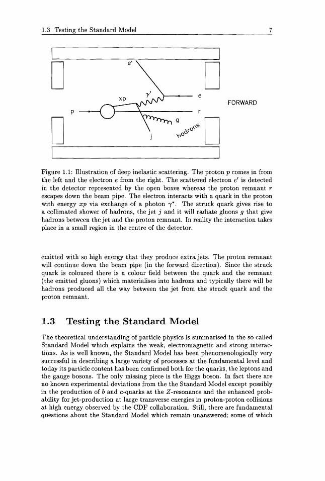
,<-,0D D Figure 1.1: Illustration of deep inelastic scattering. The proton p comes in from the left and the electron e from the right. The scattered electron e' is detected in the detector represented by the open boxes whereas the proton remnant r escapes down the beam pipe. The electron interacts with a quark in the proton with energy xp via exchange of a photon "y*. The struck quark gives rise to a collimated shower of hadrons, the jet j and it will radiate gluons 9 that give hadrons between the jet and the proton remnant. In reality the interaction takes place in a small region in the centre of the detector.

emitted with so high energy that they produce extra jets. The proton remnant will continue down the beam pipe (in the forward direction). Since the struck quark is coloured there is a colour field between the quark and the remnant (the emitted gluons) which materialises into hadrons and typically there will be hadrons produced all the way between the jet from the struck quark and the proton remnant.

1.3 Testing the Stan.dard Model

The theoretical understanding of particle physics is summarised in the so called Standard Model which explains the weak, electromagnetic and strong interac­tions. As is well known, the Standard Model has been phenomenologically very successful in describing a large variety of processes at the fundamental level and today its particle content has been confirmed both for the quarks, the leptons and the gauge bosons. The only missing piece is the Higgs boson. In fact there are no known experimental deviations from the the Standard Model except possibly in the production of band c-quarks at the Z-resonance and the enhanced prob­ability for jet-production at large transverse energies in proton-proton collisions at high energy observed by the CDF collaboration. Still, there are fundamental questions about the Standard Model which remain unanswered; some of which

8 Chapter 1 Introduction

are the subject of this thesis. One of the outstanding problems with the Standard Model is the question of

mass. One way to understand mass generation is via the Higgs mechanism but it does not explain the specific masses of the quarks and leptons. In this context the neutrinos are special since their masses are very small, if not vanishing. In the simplest version of the Standard Model they are assumed to be massless but massive neutrinos can also be accommodated within the Standard Model and the latter is believed to be true on more general theoretical grounds (see for example [Wei92J). Another special property of the neutrinos is that they carry no electric charge and this opens the question of whether they are Dirac or Majorana particles (a Majorana particle is its own antiparticle whereas a Dirac particle is different from its antiparticle). In the latter case one could observe phenomena like neutrinoless double .a-decay and lepton-number violating processes.

If the neutrinos are Majorana particles then the small neutrino mass can be understood via the so called see-saw mechanism and the addition of heavy right handed neutrinos. Such extra heavy neutrinos are not contained within the simplest version of the Standard Model but they can be present in extended versions. The possibilities of observing heavy Majorana neutrinos in Deep In­elastic Scattering (DIS) are discussed in [I] and in [VII] a Monte Carlo generator is presented which was written for this purpose.

In the Standard Model, the strong interactions are described by Quantum Chromo Dynamics (QCD). This part of the Standard Model is not so well tested as the electroweak part. The reason for this is the fact that the fundamental fields which take part in the strong interactionS, i.e. the quarks and the gluons, are not free particles but cOIifined into the hadrons which can be experimentally observed. (So far no one has been able to calculate the general hadron solutions from quarks and gluons in QCD.) However, in the high energy limit the quarks and gluons are quasi-free particles thanks to asymptotic freedom [PoI73, Gr073] and interactions between them can be calculated with so called perturbation theory.

One way of testing QCD is by studying deep inelastic scattering. The two experiments at HERA, called H1 and ZEUS respectively, have seen a remarkable increase in the probability for the electron to scatter off the proton when it interacts with small-x (x «: 1) partons in the proton. (Again x is the parton energy divided by the proton energy.) This has raised the question whether the increase is caused by a new type of dynamics for these small-x partons (called BFKL after its originators [Kur77, Ba178]) or it can be described by the same type of dynamics as for partons with higher energy fractions (called GLAP after its originators [Gri72, Alt77]). So far the data are not accurate enough to make it possible to draw any conclusions from just measuring the scattered electron so instead one has to study observables that provide more information.

One such observable is the transverse energy flow from hadrons produced in the forward hemisphere of the detector (where forward is defined as the direction of the incoming proton). Calculations at the parton level, i.e. not the observable hadron level, indicate that the transverse energy flow observed at HERA can be explained using the BFKL dynamics and that the GLAP dynamics fail in doing so. However, in [IV] it is shown that one can get a reasonable description of the

1.3 Testing the Standard Model 9

transverse energy flows in a model described in [IX] based on GLAP dynamics together with a new modelling of the proton remnant and a slightly modified hadronisation (the transition from partons to hadrons). This indicates that the range of validity for the GLAP dynamics is larger than previously expected. When the GLAP dynamics are translated into a Monte Carlo program one has to take quantum mechanical so called coherence effects into account, which are a consequence of the wave nature of the radiated partons. The observable sig­natures of coherence and how well the coherence effects are taken into account in different Monte Carlo models is discussed in [II].

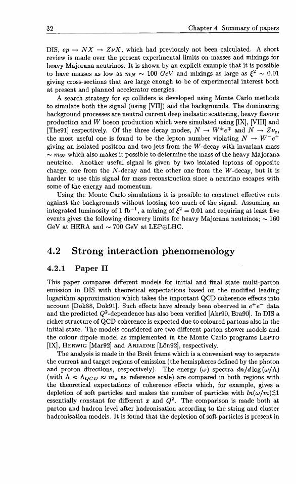
The HI and ZEUS experiments have also for the first time observed so called rapidity gap events in deep inelastic scattering. These are events where there is a large region in the forward hemisphere of the detector where no particles are observed, indicating that there is no colour connection between the struck parton system and the proton remnant. This kind of process, which was predicted by Ingelman and Schlein [Ing85], has previously been interpreted as hard scattering off a colourless object, the Pomeron, which is emitted from the proton. In [III] an alternative interpretation of this phenomenon is introduced. The process can be understood as a colour exchange between the partons that are hit by the photon and the colour medium of the proton. A concrete model implemented in [IX] of this colour changing mechanism describes the observations reasonably well as is shown in [IV].

As with all field theories, QCD has to be renormalised according to some so called renormalisation scheme to give finite predictions of physical observables. One of the consequences of the renormalisation is that the strong coupling as depends on the renormalisation scale. However, this scale is not observable and therefore all choices should be possible, which is the so called renormalisation group property. This introduces theoretical uncertainties in practical calcula­tions. The importance of taking the renormalisation scheme dependence into account when comparing experimental results and theoretical predictions is dis­cussed in [V] for jet production in deep inelastic scattering.

Several principles have been suggested for how the renormalisation scheme should be chosen, some of which are discussed in [V,VI]. In the conformal limit schemes the form of the theoretical result is similar to what one would get if the strong coupling was scale independent. In [VI] a possible extension of this kind of scheme to higher orders in the strong coupling as is presented.

The thesis is organised in the following way. In chapter 2 there is an introduc­tion to the theoretical framework of the Standard Model. Chapter 3 discusses the construction of phenomenological models in the form of Monte Carlo simu­lation programs and chapter 4 gives a short summary of the papers which the thesis is based on. Finally, chapter 5 contains the conclusions and an outlook.

At last a note on units, throughout this thesis natural units have been used, Ii = c = 1. This means that mass, momentum and energy all have the same unit, namely energy for which normally GeV is used. Time and length on the other hand both have units of inverse energy, normally GeV- l

. To convert into ordinary units one multiplies with appropriate factors of Ii = 6.582 122 x 10-25

GeV S-1 and c 299792458 m S-I.

10 1 Introduction "",u''-''IJ"""L

Chapter 2

Theoretical framework of particle physics

This chapter gives a short overview of the Standard Model of particle physics. The presentation is in no way complete; instead the purpose is to try to convey some of the basic ideas of the Standard Model, especially those that are of importance for this thesis. Apart from the specific references given the following books have also been used [Nac90, Pea94, Mut87, Dok91, Man84, Moh91, Kla88].

2.1 Introduction

The theoretical framework of the Standard Model is based on quantum field theory which is a combination of quantum mechanics and special relativity giving a Lorentz covariant theory of quantised fields.

2.1.1 The Gauge principle

The starting point of a quantum field theory is the Lagrangian density from which the equations of motion can be derived using the principle of least action. For example, the Lagrangian for a free fermion field ,¢(x) with mass m is given by

(2.1)

where 'J1. are the Dirac matrices, oJ1. = {J~I" i{J 'l/lt,o is the adjoint field, x is the space-time coordinate and J1, is the space-time index. Applying the principle of least action gives the Dirac equation,

(2.2)

which was postulated already in 1928 by Dirac [Dir28].

11

12 Chapter 2 Theoretical framework of particle physics

One of the basic principles in quantum field theory is gauge invariance, the requirement that the theory is invariant under local gauge transformations,

7jJ(X) -; U(x)7jJ(x), (2.3)

where U(x) is a unitary matrix. The Lagrangian L"" is invariant under the global transformations 7jJ(x) -; eia 7jJ(x) and i/J(x) -; e-iai/J(x) but if the transformation is local, U(x) = eia(x), then the Lagrangian transforms into,

(2.4)

which is not invariant. Gauge invariance can be restored by introducing a so called gauge field AJt(x) which transforms as

(2.5)

and that is coupled to the fermion field in the interaction Lagrangian

(2.6)

The sum of the free and the interaction Lagrangian is now invariant under the local gauge transformation. In electrodynamics, the gauge field AJt(x) is the electromagnetic field which mediates the electromagnetic interaction and e is the unit electric charge defined so that the electron charge is -e. The introduction of the gauge field in this way is normally called the minimal substitution, i.e. the derivative BJt is replaced with the covariant derivative DJt = BJt - ieAw The covariant derivative has the transformation property,

(2.7)

and thus it follows that i/J(x)DJt7jJ(x) is invariant under local gauge transforma­tions.

To complete the picture there is also a gauge invariant Lagrangian for the gauge field which is given by

LA = -~FJtll(x)FJtll(X) (2.8)

where FJtll(x) = BJtAlI(x) - BlIAJt(x). Applying the principle of least action to LA gives Maxwell's equations.

These are the only terms that respect Lorentz invariance, invariance un­der space inversion and time reversal, and renormalisability. The question of whether a term in the Lagrangian is renormalisable or not can be determined from its mass dimension d by so called power counting. Terms with d > 4 are non-renormalisable whereas terms with d ~ 4 are renormalisable. The mass dimensions for the 7jJ and AJt fields are d = 3/2 and d = 1 respectively and thus all terms in the Lagrangian considered above have dimension d = 4. The electromagnetic U(l)em symmetry is as far as is known today exact and as a consequence, the photon is massless and electric charge is conserved in all reac­tions.

2.1 Introduction 13

The Lagrangian given above is for the classical fields, i.e. they are not quan­tised. In Quantum Electro Dynamics (QED) one also needs to introduce a gauge fixing term in the Lagrangian, £GF containing the gauge fields, to be able to quantise the theory. However, this term does not contribute to any physical processes.

The above simple example reveals the beauty of the gauge principle. Starting from the matter fields 'I/J one gets the force fields associated with the gauge sym­metry by demanding invariance under local gauge transformations. The gauge principle was extended to non-Abelian symmetries, which have non-commuting transformations, by Yang and Mills in 1954 [Yan54]. The Standard Model of particle physics consists of three gauge theories which are based on different symmetries:

• electromagnetism (QED), Abelian U(l)em

• electroweak interactions, non-Abelian U(l)y ® SU(2)L

• strong interactions (QeD), non-Abelian SU(3)colour

and the respective gauge fields are the photon, the photon and the weak bosons W± and Z; and the gluons. At energies below", 100 GeV the electroweak symmetry is spontaneously broken into the electromagnetic one.

2.1.2 Perturbation theory

A very important tool in phenomenological applications of the Standard Model is the concept of perturbation theory. To illustrate the principles QED will be used as an example.

The dynamics of QED are given by the Lagrangian,

(2.9)

However, applying the principle of least action the resulting equations cannot be solved exactly due to the interaction term £1 which couples the matter and gauge fields together. If this term was absent then the Dirac and Maxwell equations would be obtained which can be solved separately. The way out of this problem is given by the smallness of the coupling e,

(2.10)

As a consequence, interactions can be considered as perturbations on the free field solutions and a reaction can be thought of as free particle propagation between certain space-time points of fundamental interactions called vertices. The theoretical predictions of physical observables then become perturbative expansions in the coupling e (or rather the coupling squared a),

(2.11)

In QED the fundamental vertices are given by £1 which connects two matter fields and a gauge field with the coupling strength e. All reactions can be built

14 Chapter 2 Theoretical framework of particle physics

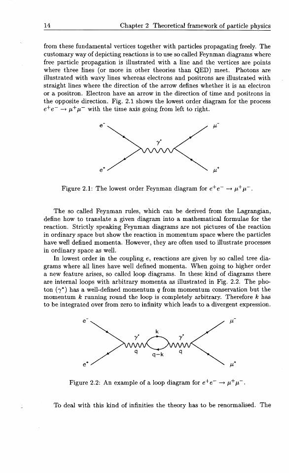
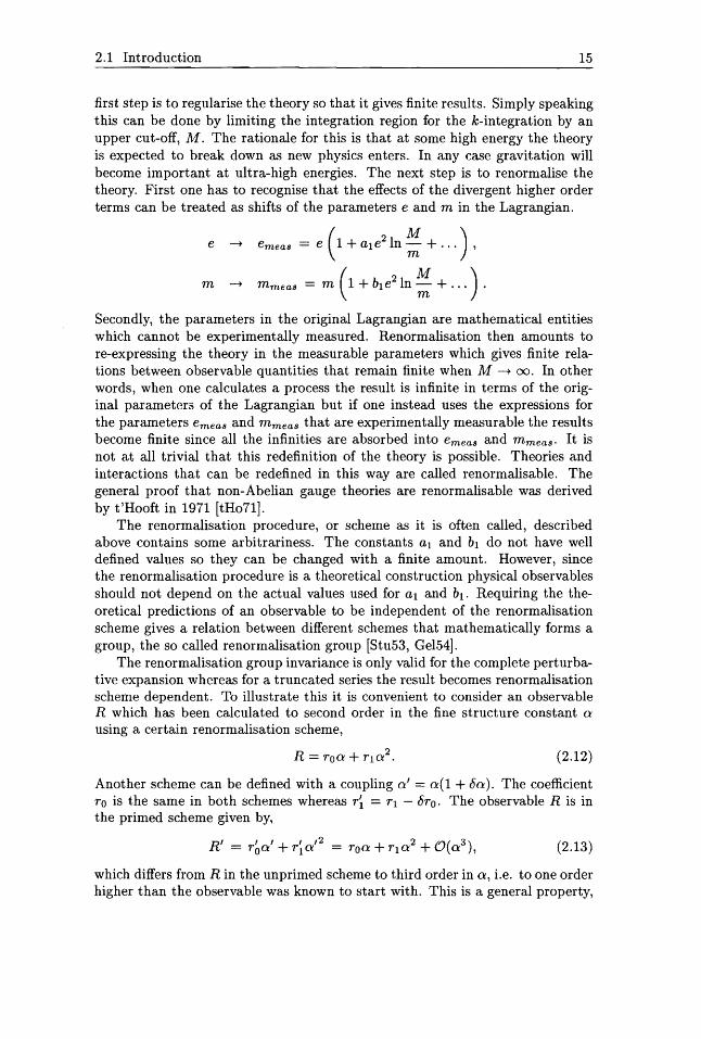
from these fundamental vertices together with particles propagating freely. The customary way of depicting reactions is to use so called Feynman diagrams where free particle propagation is illustrated with a line and the vertices are points where three lines (or more in other theories than QED) meet. Photons are illustrated with wavy lines whereas electrons and positrons are illustrated with straight lines where the direction of the arrow defines whether it is an electron or a positron. Electron have an arrow in the direction of time and positrons in the opposite direction. Fig. 2.1 shows the lowest order diagram for the process e+ e- -+ J.L+ J.L- with the time axis going from left to right.

e ~-

Figure 2.1: The lowest order Feynman diagram for -+ p,+p,-.

The so called Feynman rules, which can be derived from the Lagrangian, define how to translate a given diagram into a mathematical formulae for the reaction. Strictly speaking Feynman diagrams are not pictures of the reaction in ordinary space but show the reaction in momentum space where the particles have well defined momenta. However, they are often used to illustrate processes in ordinary space as welL

In lowest order in the coupling e, reactions are given by so called tree dia­grams where all lines have well defined momenta. When going to higher order a new feature arises, so called loop diagrams. In these kind of diagrams there are internal loops with arbitrary momenta as illustrated in Fig. 2.2. The pho­ton (,*) has a well-defined momentum q from momentum conservation but the momentum k running round the loop is completely arbitrary. Therefore k has to be integrated over from zero to infinity which leads to a divergent expression.

Figure 2.2: An example of a loop diagram for

To deal with this kind of infinities the theory has to be renormalised. The

2.1 Introduction 15

first step is to regularise the theory so that it gives finite results. Simply speaking this can be done by limiting the integration region for the k-integration by an upper cut-off, M. The rationale for this is that at some high energy the theory is expected to break down as new physics enters. In any case gravitation will become important at ultra-high energies. The next step is to renormalise the theory. First one has to recognise that the effects of the divergent higher order terms can be treated as shifts of the parameters e and m in the Lagrangian.

e -> em,., = e (1 + ale 2 In ~ + ... ) ,

m -> mmea, m (1 + b1e 2 In ~ + ... ) .

Secondly, the parameters in the original Lagrangian are mathematical entities which cannot be experimentally measured. Renormalisation then amounts to re-expressing the theory in the measurable parameters which gives finite rela­tions between observable quantities that remain finite when M -+ 00. In other words, when one calculates a process the result is infinite in terms of the orig­inal parameters of the Lagrangian but if one instead uses the expressions for the parameters emeas and mmeas that are experimentally measurable the results become finite since all the infinities are absorbed into emeas and mmeas. It is not at all trivial that this redefinition of the theory is possible. Theories and interactions that can be redefined in this way are called renormalisable. The general proof that non-Abelian gauge theories are renormalisable was derived by t'Hooft in 1971 [tH071].

The renormalisation procedure, or scheme as it is often called, described above contains some arbitrariness. The constants al and bl do not have well defined values so they can be changed with a finite amount. However, since the renormalisation procedure is a theoretical construction physical observables should not depend on the actual values used for at and bt . Requiring the the­oretical predictions of an observable to be independent of the renormalisation scheme gives a relation between different schemes that mathematically forms a group, the so called renormalisation group [Stu53, GeI54].

The renormalisation group invariance is only valid for the complete perturba­tive expansion whereas for a truncated series the result becomes renormalisation scheme dependent. To illustrate this it is convenient to consider an observable R which has been calculated to second order in the fine structure constant 0 using a certain renormalisation scheme,

(2.12)

Another scheme can be defined with a coupling 01 = 0(1 + (0). The coefficient

ro is the same in both schemes whereas r~ = rl - 8ro. The observable R is in the primed scheme given by,

RI (2.13)

which differs from R in the unprimed scheme to third order in 0, i.e. to one order higher than the observable was known to start with. This is a general property,

16 Chapter 2 Theoretical framework of particle physics

the scheme uncertainty for an observable known to order n is O(an+1 ). When a is very small, like in QED, this represents no severe problem but if a is larger, like in QCD, it becomes problematic. In QED there also exists a natural scheme choice, namely the so called on-shell scheme defined by the physical electron mass and a from the Thomson limit for Compton Scattering.

To show how well perturbation theory works it is illustrative to compare the theoretical and experimental values for the anomalous magnetic moment of the electron,

a = ge - 2

2

which is one of the best measured observables in physics. The experimental value a (1 159652 193 ± 10) x 10-12 [Mon95] agrees beautifully with the theoretical one, a = (1 159 652 201 ± 3 ± 27) x 10-12 [Kin95], which has been calculated from 981 Feynman diagrams. The first error in the theoretical value comes from numerical uncertainties in the calculation and the second from uncertainties in the experimental value of a, for which the value obtained with the quantum Hall effect has been used.

2.2 Electroweak theory

2.2.1 The electroweak Standard Model

The electroweak gauge theory, which unifies the electromagnetic and weak forces was introduced by Glashow in 1961 [Gla61]. It is based on the non-Abelian U(I)y ®SU(2)L symmetry (Y stands for hypercharge and L for left). Requiring invariance under local gauge transformation one gets four gauge fields, one for the U(I)y-symmetry, B, and three for the SU(2)L-symmetry, (WI, W 2 , W3). The gauge particles that are observed in nature are linear combinations of these fields,

A sinOwW3 + cosOwB, (2.14)

Z = COSOWW3 - sinOwB, (2.15)

W+ = ~(W1 -iW2 ), (2.16)

W- ~(W1 +iW2 ), (2.17)

where A is the photon which couples purely to the electromagnetic current and Z and W± are the weak bosons that mediate the neutral and charged current weak interactions respectively. The so called weak mixing angle (or Weinberg angle), Ow is a parameter that has to be determined from experiments.

The fermion content of the Standard Model has the following transformation properties under SU(2)L transformations (in the following, the neutrinos are not assumed to be massless since there are no theoretical reasons for doing so),

2.2 Electroweak 17

} doublets

} singlets

where each fermion is represented by a Weyl spinor. Only left-handed (L) states are affected by the weak interactions whereas the right-handed (R) states are unaffected.

The U(1)y®SU(2h gauge symmetry is not realised in nature at low energies but is spontaneously broken into the electromagnetic U(l)em symmetry. The symmetry breaking is manifest from the masses of the electroweak gauge bosons, mw± = 80 GeV and mz = 91 GeV which should be compared with the massless photon.

The standard way of explaining the electrow~ak symmetry breaking via the Higgs mechanism [Hig64] was formulated independently by Weinberg in 1967 [Wei67] and by Salam in 1968 [Sal68]. Here an extra complex scalar SU(2h doublet ¢> is introduced, the so called Higgs field, which is coupled to the gauge fields via the covariant derivative, (DJ-L¢»t (DJ-L¢». The SU(2) symmetry is broken by a nonzero vacuum expectation value of the Higgs field, < Ol¢>t ¢>IO >= v2 /2, v = 174 Ge V, that also gives rise to mass terms for the electroweak gauge fields. In a more descriptive language one can say that three of the four degrees of freedom of the Higgs field are 'eaten' by the gauge bosons which become massive. The remaining degree of freedom is a massive scalar Higgs boson H which still has not been observed.

Interactions between the Higgs field and the fermions, of so called 'Yukawa' type, is also a way of explaining the masses of the fermions which otherwise would break the U(l)y ®SU(2)L gauge symmetry. Both for the leptons and the quarks one gets terms like,

(2.18)

where h.c. stands for the Hermitian conjugate, i, j are 'family indices' which run from one to three,

tTt ('l/JiL) (veL) (2.19)'J! iL = 'IjJ~L = eL , ...

are the electroweak doublets, 'l/JjR and 'l/JjR are the electroweak singlets of up and

down type respectively, ¢ = i1'2¢>* where 1'2 is a Pauli matrix and gij, g~j are 3 x 3 matrices of Yukawa couplings. After electroweak symmetry breaking this term becomes (in unitary gauge)

(2.20)

where mij = vgij/V2 and m~j vg~j/V2 are the mass matrices for the up and down parts of the SU(2) doublets respectively. The mass matrices can

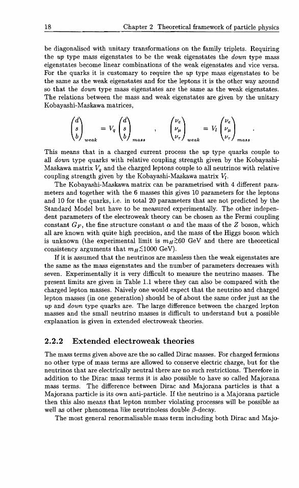
18 Chapter 2 Theoretical framework of particle physics

be diagonalised with unitary transformations on the family triplets. Requiring the up type mass eigenstates to be the weak eigenstates the down type mass eigenstates become linear combinations of the weak eigenstates and vice versa. For the quarks it is customary to require the up type mass eigenstates to be the same as the weak eigenstates and for the leptons it is the other way around so that the down type mass eigenstates are the same as the weak eigenstates. The relations between the mass and weak eigenstates are given by the unitary Kobayashi-Maskawa matrices,

(d) (d)s = Vq S

b weak b mass

This means that in a charged current process the up type quarks couple to all down type quarks with relative coupling strength given by the Kobayashi­Maskawa matrix Vq and the charged leptons couple to all neutrinos with relative coupling strength given by the Kobayashi-Maskawa matrix Vi.

The Kobayashi-Maskawa matrix can be parametrised with 4 different. para­meters and together with the 6 masses this gives 10 parameters for the leptons and 10 for the quarks, i.e. in total 20 parameters that are not predicted by the Standard Model but have to be measured experimentally. The other indepen­dent parameters of the electroweak theory can be chosen as the Fermi coupling constant GF, the fine structure constant a and the mass of the Z boson, which all are known with quite high precision, and the mass of the Higgs boson which is unknown (the experimental limit is mH2:60 GeV and there are theoretical consistency arguments that mH;S1000 GeV).

If it is assumed that the neutrinos are massless then the weak eigenstates are the same as the mass eigenstates and the number of parameters decreases with seven. Experimentally it is very difficult to measure the neutrino masses. The present limits are given in Table 1.1 where they can also be compared with the charged lepton masses. Naively one would expect that the neutrino and charged lepton masses (in one generation) should be of about the same order just as the up and down type quarks are. The large difference between the charged lepton masses and the small neutrino masses is difficult to understand but a possible explanation is given in extended electroweak theories.

2.2.2 Extended electroweak theories

The mass terms given above are the so called Dirac masses. For charged fermions no other type of mass terms are allowed to conserve electric charge, but for the neutrinos that are electrically neutral there are no such restrictions. Therefore in addition to the Dirac mass terms it is also possible to have so called Majorana mass terms. The difference between Dirac and Majorana particles is that a Majorana particle is its own anti-particle. If the neutrino is a Majorana particle then this also means that lepton number violating processes will be possible as well as other phenomena like neutrinoless double ,B-decay.

The most general renormalisable mass term including both Dirac and Majo­

2.2 Electroweak theory 19

rana mass terms is given by,

(2.21)

where VL is a three-component vector of the left-handed neutrinos from the electroweak lepton doublets and NR is a nR-component vector of right-handed electroweak singlet neutrinos (which in general can be different from three). mD is the Dirac mass term and ML and MR are the Majorana mass terms for the left and right handed neutrinos respectively.

In the standard electroweak theory Majorana mass terms are allowed but their origin is not explained. This can be done in extended electroweak theories with additional symmetries that have been broken at a scale higher than the electroweak one. For example in SO(10) theories one can have additional U(l) or SU(2)R symmetries.

If the standard electroweak theory is an effective low-energy theory, one also expects, on more general grounds, non-renormalisable terms which are sup­pressed by some large scale M like the Planck mass (see for example [Wei92]) that gives a Majorana mass matrix of the type

(2.22)

after electroweak symmetry breaking. The electroweak eigenstates VL and NR can be obtained by diagonalising the

mass matrix,

(2.23)

where ML is small and therefore has been neglected in the following. By making unitary transformations on the fields, MR can always be chosen diagonal and real which leaves mD complex and non-diagonal. Assuming that the elements of mD are much smaller than those of MR, the weak eigenstates are, for a proper choice of the fields VL, given by [Buc90]

1- ,5VL = -2-(v+~N+ ... ), (2.24)

1 +,5 T-2-(N-~ v+ ... ). (2.25)

where ~ mD/MR is the mixing between light and heavy neutrinos. This also gives the masses of the mass eigenstates N and v of the heavy and light neutrinos, respectively,

(2.26)

(2.27)

20 Chapter 2 Theoretical framework of particle physics

The last equation is the so called see-saw mechanism [Yan79, Ge180] which could explain the smallness of the neutrino mass compared with the charged leptons. If the eigenvalues of mD are much smaller than the eigenvalues of MR, then mv will be very small even if the eigenvalues of mD are of the same order of magnitude as the charged lepton masses as long as the eigenvalues of M Rare large enough. So by introducing a heavy neutrino with a mass much larger than the mass of the charged leptons it is possible to explain the small masses of the light neutrinos. The mass eigenstates v are identified with the ordinary light neutrinos and N are the heavy Majorana neutrinos, which so far have not been observed.

2.3 Quantum Chromo Dynamics

Quantum chromo dynamics is a gauge theory based on the non-Abelian SU(3)colour symmetry. There are three different charges, or colours as they are usually called, in QCD and the quark fields thus have three colour components. Since colour cannot be observed (hadrons are singlets) the underlying Lagrangian should be invariant under SU(3)colour transformations. Requiring invariance under local gauge transformations in colour space gives eight massless gauge fields, the so called gluons, that mediate the strong force. In contrast with the Abelian electro­magnetic interaction the non-Abelian electroweak and strong interactions both have self-interacting gauge fields.

2.3.1 Asymptotic freedom

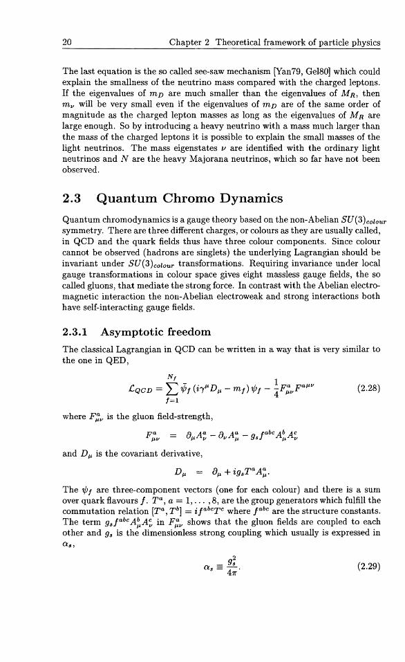
The classical Lagrangian in QCD can be written in a way that is very similar to the one in QED,

CQCD = LNf

ifif (i,1L DIL - mf) 'l/Jf - ~F:vFalLv (2.28) f=1

where F:;v is the gluon field-strength,

F a a A a a A a 9 jabcAbA CILV = IL v - v JJ. s JJ. v

and DIL is the covariant derivative,

DIL aIL + igsTaA:.

The 'l/Jf are three-component vectors (one for each colour) and there is a sum over quark flavours j. Ta, a = 1, ... ,8, are the group generators which fulfill the commutation relation [Ta, Tb] = ijabcTc where jabc are the structure constants. The term gsjabc AtA~ in F;v shows that the gluon fields are coupled to each other and gs is the dimensionless strong coupling which usually is expressed in as,

(2.29)

2.3 Quantum Chromo Dynamics 21

In addition to the terms given above there are also extra unphysical terms which are needed to quantise the theory. These terms do not contribute to any physical processes so physical predictions are still gauge invariant but the Feynman rules become gauge dependent. In all gauges except axial gauge one gets so called ghost fields but these can only exist as intermediate states.

The self-interaction between the gauge fields is the basic reason that QCD is asymptotically free, i.e. at small distances (or large energy scales) the coupling as becomes small and the quarks and gluons become quasi-free. The scale dependence of as is given by the ,8-function in the following renormalisation group equation,

dIn f.L 7r ... ,

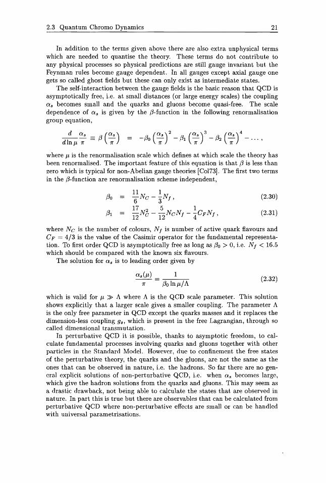
where f.L is the renormalisation scale which defines at which scale the theory has been renormalised. The important feature of this equation is that ,8 is less than zero which is typical for non-Abelian gauge theories [CoI73]. The first two terms in the ,8-function are renormalisation scheme independent,

,80 = 11 1 -Ne - -Nf6 3'

(2.30)

17 2 -Ne12

5 -NeNf12

1 - -CFNf

4 ' (2.31)

where Ne is the number of colours, Nf is number of active quark flavours and CF 4/3 is the value of the Casimir operator for the fundamental representa­tion. To first order QCD is asymptotically free as long as ,80 > 0, Le. Nf < 16.5 which should be compared with the known six flavours.

The solution for as is to leading order given by

(2.32)

which is valid for f.L ~ A where A is the QCD scale parameter. This solution shows explicitly that a larger scale gives a smaller coupling. The parameter A is the only free parameter in QCD except the quarks masses and it replaces the dimension-less coupling 9s, which is present in the free Lagrangian, through so called dimensional transmutation.

In perturbative QCD it is possible, thanks to asymptotic freedom, to cal­culate fundamental processes involving quarks and gluons together with other particles in the Standard Model. However, due to confinement the free states of the perturbative theory, the quarks and the gluons, are not the same as the ones that can be observed in nature, Le. the hadrons. So far there are no gen­eral explicit solutions of non-perturbative QCD, Le. when as becomes large, which give the hadron solutions from the quarks and gluons. This may seem as a drastic drawback, not being able to calculate the states that are observed in nature. In part this is true but there are observables that can be calculated from perturbative QCD where non-perturbative effects are small or can be handled with universal parametrisations.

22 Chapter 2 Theoretical framework of particle physics

2.3.2 Deep inelastic electron proton scattering

One process which has been analysed in detail using QCD is Deep Inelastic electron proton Scattering (DIS). The analysis can be made in two different ways, a more formal one based on the operator product expansion [Wil69] and the more intuitive QCD improved parton model [Alt77] (see also [Kog74]) based on Feynman diagrams. Here the latter formulation will be used.

Structure functions

The traditional analysis for the total DIS cross-section starts with the structure functions where only the scattered electron is observed and not the hadronic final state. The leptonic part of the reaction, illustrated in Fig. 2.3, can be calculated with QED and gives a leptonic tensor whereas the hadronic part is given by a general tensor structure, H p.v'

e'

e--....--~

q

p-----; Hadrons

Figure 2.3: The total cross-section in deep inelastic electron proton scattering.

For the total unpolarised cross-section, i.e. summing over all internal de­grees of freedom, Hp.v can only be a function of the proton momentum p and the photon momentum q. Requiring Lorentz invariance, conservation of the electromagnetic current and parity conservation limits the number of possible tensor structures to two. In turn, these two tensors can be multiplied with scalar functions of Lorentz invariant combinations of p and q. Usually these so called structure functions are denoted F1(x, Q2) and F2(X, Q2) where x = -q2/2qp and Q2 _q2. Multiplying the leptonic and hadronic tensors together gives the cross-section (neglecting the proton mass),

(2.33)

where y = xQ2js, S = (k + p)2 is the total cms energy and k is the incoming lepton momentum. By measuring the scattered electron both x and Q2 can be obtained which is sufficient to describe the inclusive cross-section. The formula given above is only valid for purely electromagnetic interactions. In the general electroweak case, taking both Wand Z exchange into account, one also gets a parity violating structure function which normally is denoted F3 . However, at small Q2 «: m~ the Wand Z exchange can be neglected compared to 1 exchange.

2.3 Quantum Chromo Dynamics 23

The parton model

In the first measurements of these structure functions it was observed that they where to a first approximation independent of the scale Q2. This so called scaling property, which had been predicted by Bjorken [Bj69a], can be inter­preted as scattering off point-like non-interacting constituents in the proton [Fey69, Bj69b], the partons as illustrated in Fig. 2.4. In this so called parton model, the total cross-section is given by the incoherent sum of the individual parton cross-sections denoted u,

du(p, q) L 10'dx Mi(Xp, q) J;(x), (2.34) ~

where Ji(x) are the parton densities. In the infinite momentum frame, x is the longitudinal momentum fraction of the parton compared to the proton assuming that the partons transverse momentum is zero.

e'

e--......---_~

Hadrons

p

Figure 2.4: Deep inelastic scattering in the parton model.

The parton model also gives a relation between the structure functions F2 and Fl which depends on the spin of the charged partons in the proton [CaI69]. For spin 1/2 one gets F2 = 2xF1 which has been experimentally confirmed and verifies that the charged partons in the proton are the quarks. The longitudinal structure function FL, given by the difference FL = F2 - 2xFl' is expected to be non-zero from QeD effects but the correction is small.

The QeD-improved parton model

To lowest order, DIS is a purely electromagnetic process and QCD only enters as a correction. Taking QCD effects into account the parton densities depend on the resolution J-LF,

du(p, q) = L 10'd~ Mi(~p, q) J;(~, I"F). (2.35) ~

When J-LF is increased, what seemed to be one parton can turn out to be sev­eral partons due to quantum fluctuations which are resolved. Fig. 2.5 illustrates

24 Chapter 2 Theoretical framework of particle physics

how DIS is pictured in this QCD-improved parton model. The scale P,F is the so called factorisation scale which defines at which scale the cross-section has been factorised into two pieces, ai and Ii. The hard part, ai, can be calcu­lated perturbatively whereas the non-perturbative part is parametrised in the parton densities. Due to the universality of mass singularities [Ama7B, E1l7B] , these parton densities are universal, i.e. the same for all processes, and can be determined from global fits of experimental data.

e' e ----+---,.--

Hadrons

p

Figure 2.5: Deep inelastic scattering in the QCD-improved parton model. (Curly lines represent gluons.)

The factorisation of the cross-section into two pieces introduces a so called factorisation scheme dependence which is similar to the renormalisation scheme dependence. First of all the scale P,F, at which the factorisation is done, is arbitrary and secondly the parton densities also have to be renormalised just as the coupling.

For not too small x the factorisation scale dependence of the parton density functions is given by the Gribov-Lipatov-Altarelli-Parisi (GLAP) [Gri72, Alt77] evolution equations,

d~(x, P,F) = ~ [ ~~ [pqq (z) ~(~,JLF) + PqG (Z) G(~'JLF)ldlnp,F

dG(x, P,F) = ~I.' ~~ [PGq(Z) ~(~,JLF) +PGGG) G(~'JLF)ldIn P,F

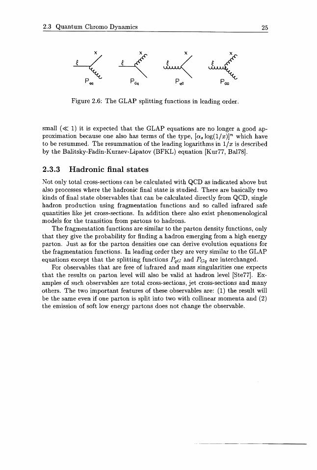
where Pqq etc are the splitting functions, G is the gluon density and ~ is the sum of the quark and antiquark densities, ~ = L:~1 (qi + qi)' The quark densities can be divided into two classes; valence quarks and sea quarks. For a baryon, the valence quarks are given by the excess of quarks compared to anti-quarks, i.e. a proton has the quark densities uv , dv , Us = Us, ds ds ) Ss = Ss etc. where the subscripts v stands for valence and s for sea. The splitting functions which are illustrated in Fig. 2.6 are known to next-to-Ieading order (NLO) [FurBO].

The GLAP equations are derived from QCD by resumming the leading terms with large logarithms in Q2 of the type, [as log(Q2)]n. When x becomes very

25 2.3 Quantum Chromo Dynamics

Figure 2.6: The GLAP splitting functions in leading order.

small «< 1) it is expected that the GLAP equations are no longer a good ap­proximation because one also has terms of the type, [O:s 10g(1/x)]n which have to be resummed. The resummation of the leading logarithms in l/x is described by the Balitsky-Fadin-Kuraev-Lipatov (BFKL) equation [Kur77, Bal78].

2.3.3 Hadronic final states

Not only total cross-sections can be calculated with QCD as indicated above but also processes where the hadronic final state is studied. There are basically two kinds of final state observables that can be calculated directly from QCD, single hadron production using fragmentation functions and so called infrared safe quantities like jet cross-sections. In addition there also exist phenomenological models for the transition from partons to hadrons.

The fragmentation functions are similar to the parton density functions, only that they give the probability for finding a hadron emerging from a high energy parton. Just as for the parton densities one can derive evolution equations for the fragmentation functions. In leading order they are very similar to the GLAP equations except that the splitting functions PqG and P Gq are interchanged.

For observables that are free of infrared and mass singularities one expects that the results on parton level will also be valid at hadron level [Ste77]. Ex­amples of such observables are total cross-sections, jet cross-sections and many others. The two important features of these observables are: (1) the result will be the same even if one parton is split into two with collinear momenta and (2) the emission of soft low energy partons does not change the observable.

- ...-- ....----------­

26 Chapter 2 Theoretical framework of particle physics

Chapter 3

Phenomenological models

Phenomenological models are important tools in high energy physics to make contact between theoretical expectations and experimental data. The usefulness is twofold: The models make it possible to transform theoretical predictions in the form of cross-section formulae into complete hadronic final states which is what is experimentally observed. These hadronic final states can then be subject to experimental cuts due to detector coverage and other limitations. The models can also be used to correct data for acceptance losses and other deficiencies in the detector system before they are compared with theoretical predictions.

An important feature in phenomenological models is the use of Monte Carlo methods to simulate different distributions. The basis for this is that the dif­ferential cross-section is essentially a probability distribution in the kinematic variables. The most widely used Monte Carlo method is so called importance sampling which can be used both to generate phase-space points from a given probability distribution and to integrate the djfferential cross-section over a cer­tain phase-space region.

3.1 Monte Carlo event generators

In a typical Monte Carlo generator the process is factorised into different phases in such a way that the dynamics of each phase can be treated independently of the others. In a deep inelastic scattering Monte Carlo (in the following we will have LEPTO described in paper [IX] in mind) the different phases are: (i) ma­trix elements calculated with perturbation theory including electroweak effects giving the hard subsystem, (ii) initial and final state parton showers based on the perturbative evolution equations giving additional parton emission, (iii) pro­ton remnant treatment and (iv) hadronisation from parametrisations or models giving a complete final state and subsequent decay of unstable hadrons. The different parts of a typical deep inelastic scattering Monte Carlo is illustrated schematically in Fig. 3.1.

27

28 Chapter 3 Phenomenological models

e -_+_----1

Hadrons

p

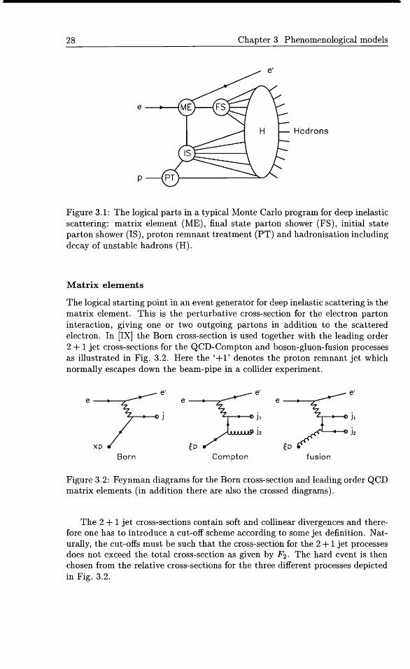
Figure 3.1: The logical parts in a typical Monte Carlo program for deep inelastic scattering: matrix element (ME), final state parton shower (FS), initial state parton shower (IS), proton remnant treatment (PT) and hadronisation including decay of unstable hadrons (H).

Matrix elements

The logical starting point in an event generator for deep inelastic scattering is the matrix element. This is the perturbative cross-section for the electron parton interaction, giving one or two outgoing partons in addition to the scattered electron. In [IX] the Born cross-section is used together with the leading order 2 + 1 jet cross-sections for the QCD-Compton and boson-gluon-fusion processes as illustrated in Fig. 3.2. Here the '+1' denotes the proton remnant jet which normally escapes down the beam-pipe in a collider experiment.

e' e' e'

Born Compton fusion

Figure 3.2: Feynman diagrams for the Born cross-section and leading order QCD matrix elements (in addition there are also the crossed diagrams).

The 2 + 1 jet cross-sections contain soft and collinear divergences and there­fore one has to introduce a cut-off scheme according to some jet definition. Nat­urally, the cut-offs must be such that the cross-section for the 2 + 1 jet processes does not exceed the total cross-section as given by F2 . The hard event is then chosen from the relative cross-sections for the three different processes depicted in Fig. 3.2.

e --+----:.,-­

xp

e --+--~

'-r---+---E) J1

./U.AA..\.AJ.r j2

'-r---+---E) j 1

J"L_~ j2

3.1 Monte Carlo event generators 29

Parton cascades

The parton cascades are divided into an initial and a final state parton shower which simulates the additional QCD radiation from the incoming and outgoing partons in the matrix element. The initial and final cascades are based on the GLAP leading log Q2 evolution equations for the parton density functions and the fragmentation functions, respectively.

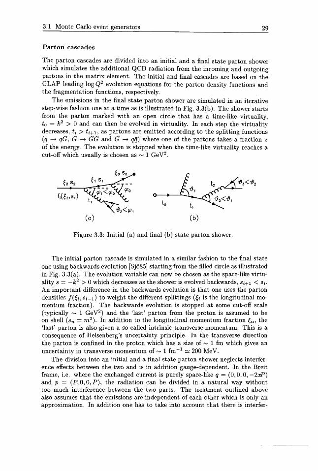
The emissions in the final state parton shower are simulated in an iterative step-wise fashion one at a time as is illustrated in Fig. 3.3(b). The shower starts from the parton marked with an open circle that has a time-like virtuality,

k 2to = > °and can then be evolved in virtuality. In each step the virtuality decreases, ti > ti+l' as partons are emitted according to the splitting functions (q -t qG, G -t GG and G -t qij) where one of the partons takes a fraction z of the energy. The evolution is stopped when the time-like virtuality reaches a cut-off which usually is chosen as "'" 1 GeV2.

(0) (b)

Figure 3.3: Initial (a) and final (b) state parton shower.

The initial parton cascade is simulated in a similar fashion to the final state one using backwards evolution [Sjo85] starting from the filled circle as illustrated in Fig. 3.3(a). The evolution variable can now be chosen as the space-like virtu­ality S = -k2 > °which decreases as the shower is evolved backwards, Si+l < Si.

An important difference in the backwards evolution is that one uses the parton densities f(ei, si-d to weight the different splittings (ei is the longitudinal mo­mentum fraction). The backwards evolution is stopped at some cut-off scale (typically 1 GeV2) and the 'last' parton from the proton is assumed to beI"V

on shell (sn = m 2 ). In addition to the longitudinal momentum fraction en, the 'last' parton is also given a so called intrinsic transverse momentum. This is a consequence of Heisenberg's uncertainty principle. In the transverse direction the parton is confined in the proton which has a size of /'"<oJ 1 fm which gives an uncertainty in transverse momentum of /'"<oJ 1 fm- 1 ~ 200 MeV.

The division into an initial and a final state parton shower neglects interfer­ence effects between the two and is in addition gauge-dependent. In the Breit frame, i.e. where the exchanged current is purely space-like q = (0,0,0, -2xP) and p (P, 0, 0, P), the radiation can be divided in a natural way without too much interference between the two parts. The treatment outlined above also assumes that the emissions are independent of each other which is only an approximation. In addition one has to take into account that there is interfer­

30 Chapter 3 Phenomenological models

ence between different emissions. These so called coherence effects can be taken into account by imposing an angular ordering of the emissions (see [Dok91] and references therein) as illustrated in Fig. 3.3.

Proton remnant treatment

To simulate the complete final state one also has to take the proton remnant into account. Normally the remnant is modelled as the three valence quarks minus the parton entering the hard interaction (initial state parton shower and matrix elements). This interacting parton can be either a valence quark, a gluon or a sea quark. In case the interacting parton is a sea quark then in addition to the valence quarks there is also the sea quark partner in the remnant to conserve quantum numbers. The partons in the remnant are then given some longitudinal and transverse momentum in a model dependent way, see e.g. [IX] for more details.

Hadronisation models

Even though no rigorous explicit non-perturbative solutions of QCD exist, at­tempts have been made to create more phenomenological models for the transi­tion from partons to hadrons, the two most common ones being the Lund string model [And83] and the cluster hadronisation model [Web84]. The hadronisation models are usually applied to the colour ordered (in the planar approximation) parton state from the parton cascades.

In the Lund model the partons are connected by a massless relativistic string representing the essentially one-dimensional colour flux between them. A typical string goes from one colour triplet charge (quark or anti-diquark) to an antitriplet charge (antiquark or diquark) with intermediate gluons represented by kinks on the string. (There can also be closed string configurations of two or more gluons in for instance T-decay.) Quark-antiquark (or diquark-antidiquark) pairs are then produced from the energy in the colour field, as described by a tunneling process. This breaks the string into a hadron and a rest-string in an iterative procedure until in the last step two hadrons are formed. In each step, the light­cone energy fraction taken by the hadron is given by a so called fragmentation function. In addition there is also some transverse momentum generated in the tunneling process which is assumed to be given by a Gaussian distribution.

In the cluster model, the first step is to split all gluons in the partonic final state into quark-antiquark pairs so that there are only triplet and anti-triplet charges in the final state. These colour charges then form pairs of colour-less clusters from the colour-ordering which decay into hadron pairs according to phase-space. For large clusters there is first a longitudinal splitting into two subclusters which is similar to the string treatment.

In both models, unstable hadrons are then decayed using information from a decay table which contains known data on lifetime and decay modes for different hadrons.

Chapter 4

Summary of papers

4.1 Search for heavy Majorana neutrinos

4.1.1 Paper I

This paper discusses the possibilities to produce and detect heavy Majorana Neutrinos at ep colliders such as the already existing HERA collider with a cms energy of Vs 314 GeV ( 30 GeV electrons on 820 GeV protons) and the possible LEPEBLHC collider with a cms energy of Vs = 1265 GeV (using the LEP electron beam of 50 GeV and the LHC proton beam of 8000 GeV).

e I,ll

W,Z

jet

p +---+--------------------R

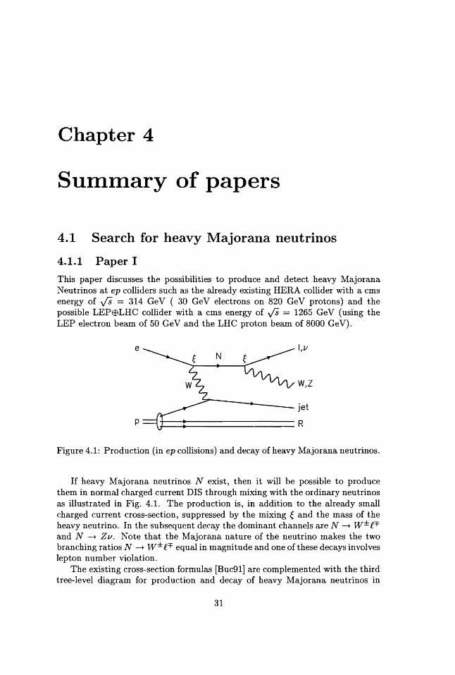
Figure 4.1: Production (in ep collisions) and decay of heavy Majorana neutrinos.

If heavy Majorana neutrinos N exist, then it will be possible to produce them in normal charged current DIS through mixing with the ordinary neutrinos as illustrated in Fig. 4.1. The production is, in addition to the already small charged current cross-section, suppressed by the mixing eand the mass of the heavy neutrino. In the subsequent decay the dominant channels are N -t W±.e::r­and N -t Zv. Note that the Majorana nature of the neutrino makes the two branching ratios N -t W±.e::r- equal in magnitude and one of these decays involves lepton number violation.

The existing cross-section formulas [Buc91] are complemented with the third tree-level diagram for production and decay of heavy Majorana neutrinos in

31

32 Chapter 4 Summary of papers

DIS, ep ~ N X ~ ZvX, which had previously not been calculated. A short review is made over the present experimental limits on masses and mixings for heavy Majorana neutrinos. It is shown by an explicit example that it is possible to have masses as low as mN '" 100 GeV and mixings as large as e '" 0.01 giving cross-sections that are large enough to be of experimental interest both at present and planned accelerator energies.

A search strategy for ep colliders is developed using Monte Carlo methods to simulate both the signal (using [VII]) and the backgrounds. The dominating background processes are neutral current deep inelastic scattering, heavy flavour production and W boson production which were simulated using [IX], [VIII] and [The91] respectively. Of the three decay modes, N ~ W±e=f and N ~ Zve ,

the most useful one is found to be the lepton number violating N ~ W- e+ giving an isolated positron and two jets from the W-decay with invariant mass '" mw which also makes it possible to determine the mass of the heavy Majorana neutrino. Another useful signal is given by two isolated leptons of opposite charge, one from the N -decay and the other one from the W -decay, but it is harder to use this signal for mass reconstruction since a neutrino escapes with some of the energy and momentum.

Using the Monte Carlo simulations it is possible to construct effective cuts against the backgrounds without loosing too much of the signal. Assuming an integrated luminosity of 1 fb- 1 , a mixing of ~2 = 0.01 and requiring at least five events gives the following discovery limits for heavy Majorana neutrinos; '" 160 GeV at HERA and", 700 GeV at LEPEBLHC.

4.2 Strong interaction phenomenology

4.2.1 Paper II

This paper compares different models for initial and final state multi-parton emission in DIS with theoretical expectations based on the modified leading logarithm approximation which takes the important QCD coherence effects into account [Dok88, Dok91]. Such effects have already been observed in e+e- data and the predicted Q2-dependence has also been verified [Akr90, Bra90]. In DIS a richer structure of QCD coherence is expected due to coloured partons also in the initial state. The models considered are two different parton shower models and the colour dipole model as implemented in the Monte Carlo programs LEPTO [IX], HERWIG [Mar92] and ARIADNE [Lon92], respectively.

The analysis is made in the Breit frame which is a convenient way to separate the current and target regions of emission (the hemispheres defined by the photon and proton directions, respectively). The energy (w) spectra dnldlog (wiA) (with A ~ AQCD ~ m7r as reference scale) are compared in both regions with the theoretical expectations of coherence effects which, for example, gives a depletion of soft particles and makes the number of particles with In(wlm)~l essentially constant for different x and Q2. The comparison is made both at parton and hadron level after hadronisation according to the string and cluster hadronisation models. It is found that the depletion of soft particles is present in

4.2 Strong interaction phenomenology 33

the models both at parton level and after hadronisation, but the expected x, Q2_ independency of the multiplicity of soft particles does not survive hadronisation.

It is also found that a good way to discriminate between the models is to look at the x- and Q2-dependence of the multiplicities in the current (nc) and target (nT) regions. The differences in the Q2 dependences of the multiplicities is most easily seen by looking at the ratio nT/nc for rat.her small x which also can be compared with the theoretical expectations. The experimental studies made at the HERA experiments have so far only studied the current region where the expected coherence effects [Der95] have been confirmed.

4.2.2 Paper III

This paper introduces soft colour interactions as a new mechanism to under­stand the relatively large fraction ( ...... 10 %) of rapidity (~ln[(E +Pz)/(E - pz)]) gap events in ep collisions as observed by the ZEUS [Der93] and HI [Ahm94] experiments. Rapidity gap events are characterised by a large region in the for­ward region (defined by the proton direction) where no particles are observed in the detector. The conventional explanation of these events is expressed in terms of scattering off a preformed colour singlet object within the proton, the Pomeron [Ing85]. Instead [III] suggests that the events can be interpreted as nor­mal hard interactions complemented with soft colour interactions which changes the colour structure of the hard subsystem in such a way that it forms a colour singlet. Being a colour singlet the hard system will hadronise separately from the proton remnant.

e'

,. , X ,. I I,,. gap

Rp ---( :t==l=~'

(a)

Figure 4.2: The string configuration in a DIS boson-gluon-fusion event: (a) conventional Lund string connection of partons, and (b) after reconnect ion due to soft colour interactions.

The new mechanism has been implemented in the Monte Carlo program LEPTO [IX]. At small-x, where the rapidity gap events have been observed, the dominating hard processes are gluon initiated as illustrated in Fig. 4.2. In the standard treatment it is assumed that the colour structure is given by the matrix element and the parton shower. Being a colour octet, the hard subsystem is then connected with two strings to the proton remnant, see Fig. 4.2(a), which makes the probability for a gap very small. The soft colour interactions may change the colour of the partons and thereby the colour topology as represented by the

(b)

34 Chapter 4 Summary of papers

strings illustrated in Fig. 4.2(b). The two strings will then hadronise separately and give the X-and R-systems with a gap in between.

The model has similar features to the observed gap events. For example, it gives a plateau in the 1Jmax-distribution, where 1Jmax is the maximum pseudo­rapidity where an energy deposition is observed in each event. The model also gives an exponential t = (p - PR)2 dependence which is similar to what is ex­pected from diffractive models. A more detailed comparison with data is made in [IV] in form of the diffractive structure function.

A new treatment of the proton remnant in events initiated by sea quarks from the proton is also introduced, which together with the soft colour interactions gives an increased forward energy flow in non-gap events in agreement with data. In case a sea quark is removed from the proton the remnant consists of the sea quark partner in addition to the valence quarks. This sea quark partner is given a longitudinal momentum using the splitting function peg ~ qij) before the momentum of the proton remnant is split into a valence-quark and a diquark. The net result is two string systems just as in a BGF-event and provides a desirable continuity between the two which reduces the dependence on the matrix element cut-off.

4.2.3 Paper IV

This paper gives a more detailed description of the observable consequences in the hadronic final state due to the soft colour interactions and the new sea quark treatment introduced in [III]. In addition, this paper also contains a discussion of different cut-off schemes for the 2 + 1 jet definition and their relation to the parton cascades as implemented in the LEPTO Monte Carlo program [IX].

It is found that a new cut-off scheme with cuts in z Pit/pq and s= (it +h)2 (it and h are the two jet momenta cf. Fig. 3.2) gives a better treatment of the singularities in the matrix element than the previously used W-scheme (Ycut W2). This way the jet cross-sections can be used in a larger part of phase-space without entering the collinear divergence regions which are better described by the parton showers. Thus the most appropriate approximation, finite order matrix element or leading log parton shower, is used in each region of the available phase-space. The distribution of partons emitted in the parton cascades is also studied and compared with the one in the Colour Dipole Model as implemented in ARIADNE [Lon92]. The resulting transverse energy flow in the hadronic final state is shown to be in good agreement with data except possibly at very small x and Q2. This means that one cannot use the hadronic energy flows to draw conclusions on whether one is observing BFKL dynamics or not.

For the rapidity gap events a new treatment of small mass strings including a valence diquark is introduced, which gives a physically more reasonable descrip­tion of the proton remnant. Calculating the diffractive structure function Ff from the simulated rapidity gap events also gives a reasonably good agreement with available data and it is shown that the charm contribution is quite small (a few percent). In a sense, the forward transverse energy flow and the rapidity gaps are orthogonal observables and it is highly non-trivial that they both can be described by the same theoretical description of the underlying dynamics.

4.3 Renormalisation scheme <:>rnh1<1r1111'u 35

4.3 Renormalisation scheme ambiguity

4.3.1 Paper V

This paper discusses the theoretical uncertainties in the next-to-Ieading-order (NLO) 2+1 jet cross-section in DIS due to the renormalisation scheme ambiguity which in NLO can be parametrised with the renormalisation scale for fixed A.

Several methods have been proposed for how the renormalisation scale should be chosen and the scale is calculated according to the following prescriptions. In the BLM method [Bro83], all {30 dependent NLO terms are absorbed into the running of as, the FAG method [Gru80] amounts to absorbing the complete NLO correction into as and the PMS method minimises the renormalisation scale dependence of the cross-section.

Since 2+1 jet-production in DIS is a multiscale problem one has to calculate the scale for different x, Q2 and Ycut values where Ycut is the resolution parameter in the jet definition, (Pi + Pi)2 = sii ~ YcutW 2 • The calculations were made with the complete O(a;) cross-section [Bro92, Gra91] for representative x, Q2

and Ycut values in the HERA kinematic range. The resulting scales are approximately proportional to Q2 whereas the x

and Ycut dependencies are more complicated. The BLM scale increases with decreasing x and increasing Ycut, which is also physically expected since the typical invariant mass of pairs of partons is given by Ycut W 2 = YcutQ21~X from the jet-definition. The FAG and PMS scales also increase with decreasing x for large Ycut, but for small Ycut the trend is the opposite. There is also an unphysical increase of the FAG and PMS scales for large x when Ycut is decreased. This indicates that the BLM scale is a better choice from a physical point of view.

To estimate the theoretical uncertainty due to the renormalisation scale de­pendence, the logarithmic derivative of the cross-section with respect to the renormalisation scale evaluated for the BLM scale was used. By choosing an appropriate value of Ycut it is possible to make the uncertainty defined in this way small. The range of useful Ycut values is Ycut 0.01 - 0.04 with the smaller f'V

value for small x and the larger one for large x. Thus, a reliable theoretical result sets both a lower and an upper limit on Ycut.

4.3.2 Paper VI

This paper discusses the possible extensions of the conformal limit arguments of the BLM method [Bro83] to fix the renormalisation scheme in next-to-next-to­leading order (NNLO). According to the conformal limit arguments, the coeffi­cients in the perturbative series of an observable should not contain any signs of scale-breaking, i.e. all the effects of {3 i= 0 should be absorbed into the running of the coupling as. In NNLO this means that there should be no {30 and fh terms present in the perturbative coefficients.

The renormalisation scheme dependence can in NNLO be parametrised with {32 and the renormalisation scale J.L (for fixed A) [Ste81]. In [VI] it is shown how one can use the conformal limit arguments to fix both the scale J.L and {32 when two observables are related, giving a commensurate {32 relation in addition to

36 Chapter 4 Summary of papers

the commensurate scale relation. The value obtained for f32 is an intermediate value between the effective charge values P2 of the two observables. This scheme fixing is also compared with other extensions of the conformal limit arguments to fix the renormalisation scale [Bro95, Bro96] in NNLO.

When applied to relations between physical observables the conformal limit arguments give unique predictions. In [VI] the arguments are applied to the relation between Re+e- and Bjorken's sum rule [Bj66] to fix both the renormali­sation scale and f32. This gives a simple relation between the two observables first noted by [Bro93] which is a perturbative version of Crewther's relation [Cre72].

Using a global fit of experimental data on Re+e- [Mar89] gives a prediction for Bjorken's sum rule which is in good agreement with the experimentally measured value [Ada95]. However, to make a more challenging test of the conformal limit arguments the experimental errors have to be much smaller. It is also shown that the general renormalisation scheme dependence for Bjorken's sum rule is quite large at the measured (Q2) = 10 GeV2 which has to be taken into account before any conclusions can be drawn.

4.4 Monte Carlo programs

The Monte Carlo generators presented in papers [VU,VIII,IX] are all written in a similar framework using FORTRAN 77. The programs consist of sets of subroutines that must be activated by the user's main steering program. The purpose of the relevant subroutines and functions are described in the respective papers together with common-block variables. Physics and programming aspects are also described in the papers.

All programs use the importance sampling method to generate phase-space points from the respective matrix-elements where different parametrisations of parton density functions can be used. Higher order QCD-radiation is added using initial and final state parton showers. A complete hadronic final state of observable particles is then produced using the Lund string hadronisation model [And83] as implemented in the Monte Carlo program JETSET [Sj593]. Thus, the complete 'history' of the event is generated resulting in a complete final state.

The programs described in [VIII] and [IX] also contain an implementation of the soft colour interaction mechanism presented in [III] which can give rise to rapidity gap events and exclusive vector-meson production (in particular J /iI!).

4.4.1 Paper VII: MAJOR

This paper contains a presentation of a Monte Carlo generator which has been constructed to simulate the production and decay of heavy Majorana neutrinos via lepton mixing. The generator is based on the importance sampling method to simulate the complete differential cross-section formula for the processes ep ~ N X ~ e±W=fX or veZX, both for incoming electrons and positrons. The program has also been modified to simulate the production of right-handed neutrinos through the exchange of right-handed W-bosons WR, see e.g. [Buc92},

4.4 Monte Carlo programs 37

under the assumption that the WR is lighter than the heavy neutrino and that there is no mixing with Standard Model gauge bosons.

4.4.2 Paper VIII: AROMA

This paper describes a program to simulate the production of heavy quarks through the boson-gluon fusion process in e±p collisions. The full electroweak structure of the electron-gluon interaction is taken into account as well as the masses of the produced heavy quarks using the cross-section formula in [Sch88]. The program uses the general purpose program DIVONNE [Fri81] to generate phase-space points from the differential cross-section formula with the impor­tance sampling method.

4.4.3 Paper IX: LEPTO

Physics and programming aspects are discussed for a Monte Carlo program to simulate complete events in deep inelastic lepton-nucleon scattering. The parton level interaction is based on the standard model electroweak cross sections, which are fully implemented in leading order for any lepton of arbitrary polarisation. In addition to the Born cross-section, the first order QCD matrix elements for gluon radiation and boson-gluon fusion are also implemented with different cut­off schemes.

38 Chapter 4 Summary of papers

Chapter 5

Conclusions and outlook

Quarks and leptons are today thought of as the fundamental constituents of matter and their interactions are described by the Standard Model of particle physics.

The neutrinos are very special in the Standard Model. They only interact with the weak interaction and they have been found to be almost massless. If heavy Majorana neutrinos exist they can explain the smallness of the light neutrino masses through the see-saw mechanism. As this thesis has shown, an efficient way to search for heavy Majorana neutrinos is provided by deep inelastic scattering experiments at electron-proton colliders. The discovery limits are, for a mixing of 1% and an integrated luminosity of 1 fb- 1 , about 160 GeV at HERA and 700 Ge V at LEPEBLHC, a possible combination of the LEP and LHC accelerators at CERN.

The strong interactions are in the Standard Model described by Quantum Chromo Dynamics (QCD). Deep inelastic scattering offers new possibilities of testing QCD, for example by studying the hadronic final state. Quantum me­chanical coherence effects have already been observed in the current jet region but an even richer structure is expected in the proton remnant region which so far has not been observed.

By studying the transverse energy flow there has been hope that one could learn more about QCD dynamics in the small-x region which presently is probed by the HERA experiments. But as this thesis has shown, the observations made so far can be explained with ordinary GLAP dynamics together with non-perturbative hadronisation effects and does not require the small-x BFKL dynamics.

Another testing ground for QCD dynamics is given by the rapidity gap phe­nomenon observed by the HERA experiments. In the soft colour interaction model this kind of events are interpreted as an ordinary hard interaction supple­mented with colour rearrangements which only effects the colour structure of the final state. Comparing the model with available data in form of the diffractive structure function shows a reasonably good agreement.

When comparing experimental data with theoretical predictions one must take the theoretical uncertainties into account as emphasised in this thesis. This

39

40 Chapter 5 Conclusions and outlook

is especially important in QCD where the renormalisation scheme dependence is large. For the 2 + 1 jet cross-section, the renormalisation scheme ambiguities give a theoretical uncertainty which limits the range of jet cut-oft's that can be used.

The conformal limit arguments can be used to fix the renormalisation scheme in a unique way when two observables are related by requiring all signs of scale breaking ({3 -I 0) to be absorbed into the scale dependence of the strong coupling as. This thesis has shown how the conformal limit arguments can be extended to NNLO to fix both the renormalisation scale and {32. The resulting {32 is an intermediate value between the ~2 's of the two observables that are related.

Even though the Standard Model has been phenomenologically very success­ful, there are fundamental questions which remain to be answered. For example, all the matter in the Universe today consists of u and d-quarks and electrons so why are there three generations of fundamental particles. Another problem is related to the Higgs mechanism for mass generation. According to this mecha­nism there should also be another particle, the Higgs boson, but it has not been observed yet. From the large variation in masses one could perhaps also suspect that the quarks and leptons are composite objects. This intriguing possibility may also be the explanation of the increased jet cross-section observed by the CDF experiment in proton anti-proton collisions at Fermilab's Tevatron.

Presently a new large proton collider (LHC) is being constructed at CERN which will collide protons with about seven times more energy than the Tevatron. This will provide new answers about the fundamental structure of matter and whether the Higgs boson exists. Going to even higher energies it is not so evident what will happen. There are strong theoretical reasons to believe that the Standard Model will break down when the energy is increased and there are theories beyond the Standard Model which attempts to describe new physics at such energies.

Acknowledgements

First of all I want to thank my supervisor Gunnar Ingelman for all his support and encouragement during my years as Ph.D. student and for introducing me to the fascinating world of phenomenological particle physics. Thanks also for providing the invaluable connection with the inspiring research atmosphere at DESY in Hamburg, both the theory group and the HERA experiments, and for making it possible for me to attend summer schools, workshops and conferences already in the beginning of my Ph.D. studies.

I would like to thank the other high energy physicists at the department for creating a nice working atmosphere. Special thanks to my room-mate Anders Edin for useful and sometimes endless discussions about particle physics and for collaboration on some of the papers in this thesis. Thanks to Ib Koersner and Roger Ruber for keeping the computer system running and the secretarial staff for taking care of administrative problems. Thanks also to Sven Kullander for his generous leadership of high energy physics at the department which has made this line of research possible.

My sincere thanks to Stan Brodsky for helpful discussions about the au­tomatic scale fixing method and the application of conformal limit arguments. I also want to thank Erwin Mirkes for helpful discussions on the next-to-Ieading­order calculation of the 2+1 jet cross-section. Many thanks to Wilfred Buchmiiller and Christoph Greub for their guidance on the more theoretical aspects of heavy Majorana neutrinos.

Thanks to Frank Kole for helpful information about the capabilities of the HI detector to detect isolated electrons and positrons and for running the W­background Monte Carlo. I also want to thank Leif Jonsson, .Morten Nyberg­Werther and Christian Jacobsson in the Lund HI group for helpful discussions about experimental results on the hadronic final state and for useful feedback on the performance of the LEPTO Monte Carlo. Thanks also to Christophe Royon and Nick Brook for helpful discussions about experimental results from the HERA experiments.

Finally I want to thank the Swedish Natural Science Research Council for providing the funds that made this endeavour possible.

41

42

Bibliography

[Aba95] S. Abachi et al. (DO ColI.), Phys. Rev. Lett. 74 (1995) 2632.

[Abe95] F. Abe et al. (CDF Coll.), Phys. Rev. Lett. 74 (1995) 2626.

[Abe96] F. Abe et al. (CDF ColI.), 'Inclusive jet cross section in pp at .JS = 1.8 TeV', FERMILAB-PUB-96-020-E, Jan 1996, hep-ex/9601008.

[Ada95] D. Adams et al. (SMC ColI.), Phys. Lett. B357 (1995) 248.

[Ahm94] T. Ahmed et al. (HI colI.), Nucl. Phys. B429 (1994) 477; Phys. Lett. B348 (1995) 681

[Akr90] M. Z. Akrawyet al. (OPAL coll.), Phys. Lett. B247 (1990) 617.

[Alt77] G. Altarelli and G. Parisi, Nucl. Phys. B 126 (1977) 298.

[Ama78] D. Amati, R. Petronzio and G. Veneziano, Nucl. Phys. B 146 (1978) 29

[And32] C. D. Anderson, Science 76 (1932) 238.

[And33] C. D. Anderson, Phys. Rev. 43 (1933) 491.

[And37] C. D. Anderson, Phys. Rev. 51 (1937) 884.

[And38] C. D. Anderson and S. Neddermeyer, Phys. Rev. 54 (1938) 88.

[And83] B. Anderson et al., Phys. Rep. 97 (1983) 31.

[Arn83] G. Arnison et al. (UAI colI.), Phys. Lett. 122B (1983) 103; Phys. Lett. 126B (1983) 398.

[Aub74] J. J. Aubert et al., Phys. Rev. Lett. 33 (1974) 1404.

[Aug74] J. E. Augustin et al., Phys. Rev. Lett. 33 (1974) 1406.

[Bag83] P. Bagnaia et al. (UA2 colI.), Phys. Lett. 129B (1983) 130.

[BaI78] Va. Va. Balitsky and L. N. Lipatov, Sov. J. Nucl. Phys. 28 (1978) 822.

[Ban83] D. P. Banner et al. (UA2 colI.), Phys. Lett. 122B (1983) 476.

43

44 Bibliography

[Bar80]

[Ber79]

[Bj66]

[Bj69a]

[Bj69b]

[Bra80]

[Bra90]

[Bre69]

[Bro83]

[Bro92]

[Bro93]

[Bro95]

[Bro96]

[Buc90]

[Buc91]

[Buc92]

[Cal69]

[Cha32]

[Co173]

[Cre72]

[Der93]

[Der95]

[Dir28]

W. Bartel et al. (JADE CoIl.), Phys. Lett. 91B (1980) 142.

C. Berger et al. (PLUTO CoIl.), Phys. Lett. 86B (1979) 418.

J. D. Bjorken, Phys. Rev. 148, 1467 (1966); Phys. Rev. D 1, 1376 (1970).

J. D. Bjorken, Phys. Rev. 179 (1969) 1547.

J. D. Bjorken and E. A. Paschos, Phys. Rev. 185 (1969) 1975.

R. Brandelik et aL (TASSO CoIl.), Phys. Lett. 97B (1980) 453.

W. Braunschweig et al. (TASSO CoIL), Z. Phys. C 47 (1990) 187.

M. Breidenbach et al., Phys. Rev. Lett. 23 (1969) 935.

S. J. Brodsky, G. P. Lepage, P. B. Mackenzie, Phys. Rev. D 28 (1983) 228.

T. Brodkorb, J. G. Korner, Z. Phys. C 54 (1992) 519, T. Brodkorb, J. G. Korner and E. Mirkes, Nuc1. Phys. B 29A (1992) 144, T. Brodkorb and E. Mirkes, Z. Phys. C 66 (1995) 141; preprint MAD/PH/821 (1994).

D. J. Broadhurst and A. L. Kataev, Phys. Lett. B 315 (1993) 179.

S. J. Brodsky and H. J. Lu, Phys. Rev. D 51 (1995) 3652.

S. J. Brodsky, G. T. Gabadadze, A. L. Kataev and H. J. Lu, DESY preprint 95-245, e-Print Archive hep-ph/9512367.

W. Buchmiiller and D. Wyler, Phys. Lett. B 249 (1990) 458.

W. Buchmiiller' and C. Greub, Phys. Lett. B256 (1991) 465; Nuc1. Phys. B 363 (1991) 345.

W. BuchmiiIler and C. Greub, Nucl. Phys. B381 (1992) 109.

C. G. Callan, Jr. and D. J. Gross, Phys. Rev. Lett. 22 (1969) 156.

J. Chadwick, Proc. Roy. Soc. London A136 (1932) 692.

S. Coleman and D. J. Gross, Phys. Rev. Lett. 31 (1973) 85!.

R. J. Crewther, Phys. Rev. Lett. 28 (1972) 1421

M. Derrick et aI. (ZEUS Coll.), Phys. Lett. B315 (1993) 481; Z. Phys. C 68 (1995) 569.

M. Derrick et al. (ZEUS Coll.), Z. Phys. C 67 (1995) 93.

P. A. M. Dirac, Proc. Roy. Soc. London A117 (1928) 610.

45 Bibliography

[Dok91] Yu. L. Dokshitzer et aL, 'Basics ofperturbative QCD', Editions Fron­tieres 1991.

[Dok88] Yu. L. Dokshitzer et al., Rev. Mod. Phys. 60 (1988) 373 L. V. Gribov et aI., Sov. Phys. JETP 68 (1988) 1303.

[Ein05] A. Einstein, Ann. Phys. (Leipzig) 17 (1905) 132.

[E1l78] R .. K. Ellis et al., Phys. Lett. 78B (1978) 281; Nucl. Phys. B 152 (1979) 285.

[Fey69] R. P. Feynman, Phys. Rev. Lett. 23 (1969) 1415.

[Fri81] J. Friedman and M. Wright, ACM Trans. Math. Software 7 (1981) 76, DIVONNE 4, CERN library program D151.

[Fur80] W. Furmanski, R. Petronzio, Phys. Lett. 97B (1980) 437.

[GeI54] M. Gell-Mann and F. E. Low, Phys. Rev. 95 (1954) 1300.

[GeI64] M. Gell-Mann, Phys. Lett. 8 (1964) 214.

[GeI80] M. Gell-Mann, P. Ramond and R. Slasky, in Supergravity, ed. P. van Nieuwenhuizen, (North Holland, Amsterdam 1980).

[Gla61] S. L. Glashow, Nucl. Phys. 22 (1961) 579.

[Gra91] D. Graudenz, Phys. Lett. B256 (1991) 518; Phys. Rev. D49 (1994) 3291; Compo Phys. Commun. 92 (1995) 65.

[Gri72] V. N. Gribov, 1. N. Lipatov, Sov. J. Nucl. Phys. 15 (1972) 438.

[Gro73] D. J. Gross, F. Wilczek, Phys. Rev. Lett. 30 (1973) 1343.

[Gru80] G. Grunberg: Phys. Lett. B 95 (1980) 70; Phys. Lett. B 110 (1982) 501; Phys. Rev. D 29 (1984) 2315.

[Her77] S. W. Herb et al., Phys. Rev. Lett. 39 (1977) 252.

[Hig64] P. W. Higgs, Phys. Rev. Lett. 13 (1964) 508.

[Ing85] G. Ingelman, P. E. Schlein, Phys. Lett. B152 (1985) 256.

[Kin95] T. Kinoshita, Phys. Rev. Lett. 75 (1995) 4728, and references therein.

[Kla88] 'Neutrinos', Ed. H. V. Klapdor, Springer Verlag 1988.

[Kog74] J. Kogut and L. Susskind, Phys. Rev. D9 (1974) 697; 3391.

[Kur77] E. A. Kuraev, L. N. Lipatov and V. S. Fadin, Sov. Phys. JETP 45 (1977) 199.

[Lon92] L. Lonnblad, Comput. Phys. Commun. 71 (1992) 15.

46 Bibliography

[Man84] F. Mandl, G. Shaw, 'Quantum Field Theory', John Wiley & Sons 1984.

[Mar89] R. Marshall, Z. Phys. C 43 (1989) 595.

[Mar92] G. Marchesini et al., Comput. Phys. Commun. 67 (1992) 465.

[Moh91] R. N. Mohapatra, P. B. Pal, 'Massive neutrinos in physics and astro­physics', World Scientific 1991.

[Mut87] T. Muta, 'Foundations of Quantum Chromodynamics', World Scien­tific 1987.

[Nac90] o. Nachtmann, 'Elementary Particle Physics', Springer Verlag 1990.

[Mon95] L. Montanet et al., Phys. Rev. D50 (1994) 1173.

[Pau40] W. Pauli, Phys. Rev. 58 (1940) 716.

[Pea94] 'High Energy Phenomenology', Ed. K. J. Peach and L. L. J. Vick, Institute of Physics Publishing 1994.

[Per75] M. L. Perl et al., Phys. Rev. Lett. 35 (1975) 1489.

[PoI73] H. D. Politzer, Phys. Rev. Lett. 30 (1973) 1346.

[Rei53] F. Reines and C. L. Cowan, Jr., Phys. Rev. 92 (1953) 830.

[Rei56] F. Reines et al., Science 124 (1956) 103.

[Rei59] F. Reines and C. L. Cowan, Jr., Phys. Rev. 113 (1959) 273.

[Rhu11] E. Rutherford, Phil. Mag. 21 (1911) 669.

[Rhu19] E. Rutherford, .Phil. Mag. 37 (1919) 581.

[SaI68] A. Salam, in Proc. of the 8th Nobel Symposium, ed. N. Svartholm, (Almqvist & Wiksell, Stockholm, 1968).

[Sch88] G. A. Schuler, Nucl. Phys. B299 (1988) 21.

[Sjo85] T. Sjostrand, Phys. Lett. 157B (1985) 321.

[Sjo93] T. Sjostrand, PYTHIA 5.7 and JETSET 7.4, CERN-TH.7112/93; Compo Phys. Comm. 82 (1994) 74.

[Ste77] G. Sterman and S. Weinberg, Phys. Rev. Lett. 39 (1977) 1436.

[Ste81] P. M. Stevenson, Phys. Lett. B 100 (1981) 61, Phys. Rev. D 23 (1981) 2916, Nucl. Phys. B 203 (1982) 472, Nucl. Phys. B 231 (1984) 65.

[Str37] J. C. Street and E. C. Stevenson, Phys. Rev. 52 (1937) 1003.

[Stu53] E. C. G. Stiickelberg and A. Petermann, Helv. Phys. Acta 26 (1953) 499.

47 Bibliography

[The91] E. Theuer, 'Monte Carlo Untersuchungen der W-boson Produktion und konkurierender Prozesse bei HERA', Diplomarbeit, Technische Hochschule Aachen (1991).

[Tho97] J. J. Thomson, Phil. Mag. 44 (1897) 269.

[tHo71] G. t'Hooft, NucL Phys. B33 (1971) 173.

[Web84] B. R. Webber, NucL Phys. B238 (1984) 492 G. Marchesini and B. R. Webber, Nuel. Phys. B238 (1984) 1.

[Wei67] S. Weinberg, Phys. Rev. Lett. 19 (1967) 1264.

[Wei92] S. Weinberg, in Proc. of the XXVI Int. Conf. on High Energy Physics, (1992), ed. J. Sanford, (AlP, New York, 1993), p. 346.

[Wi169] K. G. Wilson, Phys. Rev. 179 (1969) 1499.

[Yan54] C. N. Yang and R. Mills, Phys. Rev. 96 (1954) 191.

[Yan79] T. Yanagida, in Proc. of the Workshop on the Unified Theory and the Baryon Number of the Universe, KEK 1979

[Zwe64] G. Zweig, CERN-Report TH-401 and TH-412.