Quartzdyne Inc. Quartz Transducer Drift Characterization

Joel Linford M.S.

August 17, 2016

Abstract

The Quartzdyne pressure transducer isrenowned in the down hole oil industry forits long term reliability and performance. Dueto the long life expectancy of Quartzdyneproducts, the drift of sensors is a value ofgreat interest to the end user. While the driftat maximum conditions is specified to be lessthan 0.02 %F.S. per year, questions regardingthe typical drift at non maximum conditionshave arisen. This document discusses a studyperformed by Quartzdyne inc., designed toquantify the expected drift of a Quartzdynetransducer when operating under a variety ofpressure and temperature conditions. In thisstudy, more than 160 transducers were testedover a range of pressures and temperatures,amounting to more than 20,000 unit-test-hours.

1 Background

The Quartzdyne pressure transducer isrenowned in the down hole oil industry forit’s long term reliability and performance.Among extreme accuracy, resolution, andruggedness, the minimal drift of the transducerenabled Quartzdyne’s quartz pressure sensingto become industry standard.

In the early 2000’s Quartzdyne began to opti-

mize the long term stability of its quartz pressuresensor. By late 2002, through design and processchanges discovered through extensive research,the drift of a pressure sensor had been reducedby more than a factor of two, creating one ofthe most stable pressure sensors used in the oilindustry [2]. Since that time, Quartzdyne hasremained dedicated to maintaining and improv-ing the performance of its sensors, to secure itsposition as an industry standard.

2 Motivation

In 2002, the specifications for a Quartzdynequartz transducer were set to be less than 0.02%F.S. per year when operating under maximumpressure and temperature conditions. Manyusers of the product however do not operate un-der maximum conditions, instead operating atlower pressures and temperatures. Due to this,interest arose as to the expected drift under avariety of conditions.

It is known that variation in the manufactur-ing of a product will induce a distribution of pos-sible outputs, causing the specified drift to oftenbe much greater than the average. Customer in-terest also arose in the expected drift and thevariation therein.

In response to these interests, Quartzdyne de-signed this study. The study, as described in

1

detail below, varied pressure and temperature,measuring the drift of multiple units, in an at-tempt to quantify expected values correspondingto these inputs.

3 Testing

This study consisted of a compilation of multiplestability tests, wherein, the drift of the Quartz-dyne pressure gauge was measured. When mea-suring drift, care must be taken as the de-gree of measurement becomes comparable to, orless than the fluctuations in atmospheric condi-tions. Precise monitoring of atmospheric condi-tions must accompany the sensor readings to en-able the subtraction of non drift deviation fromthe measurement.

The stability tests were performed using thefollowing equipment. A DH Instruments 5306Manual Deadweight tester, accurate to 0.01%of reading was used to read pressure. A ThetaSystems PM170 Series Hydraulic Pressure Con-troller was used to maintain pressure. A CascadeTEK forced air oven was used to apply tempera-ture. Atmospheric pressure was monitored witha Mensor DPG 2400 Barometer. An Azonix Her-metic Resistor was used to monitor the DH pis-ton temperature. Quartzdyne QCOM hardwareand software was used to monitor the Quartz-dyne Pressure transducers, the devices undertest.

To increase the temperature stability, theunits were placed in an aluminum cylinder whichwas then filled with small steel balls creating alarge thermal mass. This thermal mass damp-ened the fluctuations in the oven causing a tem-perature stability of ±0.02◦C from the oven setpoint.

The procedure used when running these tests

is as follows. Only newly built and calibratedtransducers were used. This ensured that thetest accurately depicted the drift to be expectedby a customer. The units were placed on a pres-sure manifold, and submerged in a thermal mass,which was then placed in the oven. The trans-ducers were connected to QCOM hardware viahigh temperature cables, and the manifold wasconnected to the Deadweight via a pressure line.The system was then heated to the desired testtemperature and allowed to stabilize. Once thetemperature had stabilized, data collection at arate of 1 min was started, and pressure was ap-plied. The system was allowed to run for a pe-riod of five to seven days, at which point, datacollection was halted. Pressure was removed andthe system allowed to cool. Week long test pe-riods were selected because both short and longterm effects were sufficiently visible within thistime frame.

Over 30 tests were run. The 10K sensor typedrift was examined under all combinations ofpressure and temperature with temperatures of100◦C, 125◦C and 150◦C and pressures of 6kpsi,8kpsi and 10kpsi. The 16K sensor type wasdrifted under all combinations of pressure andtemperature consisting of temperatures 125◦C,150◦C and 175◦C, and pressures ranging from10kpsi to 16kpsi in steps of 2kpsi. The 20Ksensor type was tested at the same temperaturesas the 16K but the pressures were increased to18kpsi and 20kpsi.

4 Analysis

4.1 Drift

As mentioned above, one must be thoughtfulwhen calculating drift, to remove all non relateddeviation in the pressure measurement. This is

2

done though the use of the true absolute pres-sure calculation, which is explained in Calibra-tion Procedures & Metrology Uncertainties [1].The drift calculated in this paper is defined byEq:1.

~D = ~PS − ~PT − PS (0)− PT (0) . (1)

~D denotes the drift vector, ~PS denotes the vectorof pressure sensor readings, ~PT denotes the vec-tor of true absolute pressure values. PS(0) andPT (0) denote the initial element of their corre-sponding vectors. A moving average filter wasapplied to the drift vector to remove randomvariation caused by minute time differences be-tween ~PS and ~PT . An example of this calculationis shown in figure 1.

Figure 1: The removal of noise caused by at-mospheric pressure and temperature deviations,through the subtraction of calculated true pres-sure from the sensor readings to yield sensordrift.

4.2 Fitting

Fitting these data is required to project the driftand obtain a annual anticipated drift. The for-

mula used to fit and project drift in this studyis described in Eq:2.

d(t) = A1

(e− tτ1 − 1

)−A2 ln

(t

τ2+ 1

). (2)

A1, τ1, A2, and τ2 are constants to be manipu-lated to fit the data. It will be helpful to breakup Eq:2 into two separate equations (Eq:3, Eq:4)for the sake of discussion.

drapid(t) = A1

(e− tτ1 − 1

). (3)

dslow(t) = −A2 ln

(t

τ2+ 1

). (4)

Eq:3 describes the rapid exponential portion ofdrift. This rapid decay is commonly depletedwithin the fist day or so of the drift test, andcan be either positive or negative. Please notethat,

limt→∞

drapid(t) = −A1, (5)

andlimt→0

drapid(t) = 0. (6)

Eq:4 describes the long term drift of the trans-ducer. This form of drift modeling is well ac-cepted for quartz resonators and other typesof mechanical stress relaxation [6]. Please alsonote,

limt→∞

dslow(t) = ±∞, (7)

depending on the sign of A2,

limt→0

dslow(t) = 0, (8)

and

limt→∞

d

dtdslow(t) = 0. (9)

Eq:2 therefore describes the sensor as ever drift-ing and the drift rate is ever decreasing. Thisequation provides a remarkably good fit for the

3

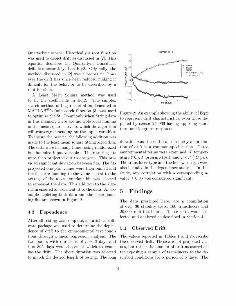
Quartzdyne sensor. Historically a root functionwas used to depict drift as discussed in [2]. Thisequation describes the Quartzdyne transducerdrift less accurately than Eq:2. Originally, themethod discussed in [2] was a proper fit, how-ever the drift has since been reduced making itdifficult for the behavior to be described by aroot function.

A Least Mean Square method was usedto fit the coefficients in Eq:2. The simplexsearch method of Lagarias et al implemented inMATLAB R©’s fminsearch function [3] was usedto optimize the fit. Commonly when fitting datain this manner, there are multiple local minimain the mean square curve to which the algorithmwill converge depending on the input variables.To ensure the best fit, the following addition wasmade to the least mean square fitting algorithm.The data were fit many times, using randomizedbut bounded input variables. The resulting fitswere then projected out to one year. This pro-vided significant deviation between fits. The fitsprojected one year values were then binned andthe fit corresponding to the value closest to theaverage of the most abundant bin was selectedto represent the data. This addition to the algo-rithm ensured an excellent fit to the data. An ex-ample depicting both data and the correspond-ing fits are shown in Figure 2.

4.3 Dependence

After all testing was complete, a statistical soft-ware package was used to determine the depen-dence of drift to the environmental test condi-tions through a linear regression analysis. Thetwo points with durations of t = 6 days andt = 365 days were chosen at which to exam-ine the drift. The short duration was selectedto match the desired length of testing. The long

0 1 2 3 4 5−0.4

−0.3

−0.2

−0.1

0

0.1

0.2

0.3Example of Fit

Time (days)

Pre

ssur

e D

rift (

psi)

246873246907246966Fit: A

1(exp(−t/τ

1) − 1)

−A2 ln(t/τ

2 + 1)

Figure 2: An example showing the ability of Eq:2to represent drift characteristics, even those de-picted by sensor 246966 having apposing shortterm and longterm responses.

duration was chosen because a one year predic-tion of drift is a common specification. Threeenvironmental terms were examined. T temper-ature (◦C), P pressure (psi), and T ×P (◦C psi).The transducer type and the bellows design werealso included in the dependence analysis. In thisstudy, any correlation with a corresponding p-value ≤ 0.05 was considered significant.

5 Findings

The data presented here, are a compilationof over 30 stability tests, 160 transducers and20,000 unit-test-hours. These data were col-lected and analyzed as described in Section 4.

5.1 Observed Drift

The values reported in Tables 1 and 2 describethe observed drift. These are not projected val-ues, but rather the amount of drift measured af-ter exposing a sample of transducers to the de-scribed conditions for a period of 6 days. The

4

values reported are the mean (µ) and standarddeviation (σ) of the absolute drift of the testedsamples.

For those who are unfamiliar with this methodof reporting uncertainty, the form µ(σ) corre-sponds to µ± σ where sigma is weighted at theindicated significance i.e. 0.36(14)→ 0.36±0.14.

Absolute drift was reported because theQuartzdyne sensor has been optimized to driftabout zero. Due to this, test results were a mixof positive and negative values. Looking at devi-ation from zero, allowed comparisons to be madewith smaller sample sizes than would have oth-erwise been required.

Table 1: 10K Sensor Type, 6 Day ObservedMean Absolute Drift (psi)

P(kpsi) 100◦C 125◦C 150◦C 175◦C

6 0.10(5) 0.33(18) 0.17(4) -8 0.18(10) 0.21(5) 0.33(14) -10 0.42(16) 0.51(20) 0.17(5) 0.14(11)

Errors correspond to one standard deviation.

Table 2: 16K & 20K Sensor Types, 6 Day Ob-served Mean Absolute Drift (psi)

P (kpsi) 125◦C 150◦C 175◦C

10 0.12(3) 0.15(3) 0.07(7)12 0.36(14) 0.16(6) 0.50(27)14 0.12(7) 0.07(8) 0.12(8)16 0.33(24) 0.22(11) 0.08(6)18 0.36(17) 0.10(6) 0.29(18)20 0.43(28) 0.25(19) 0.51(38)

Errors correspond to one standard deviation.

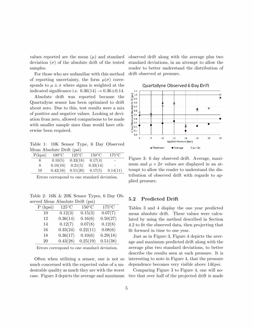
Often when utilizing a sensor, one is not somuch concerned with the expected value of a un-desirable quality as much they are with the worstcase. Figure 3 depicts the average and maximum

observed drift along with the average plus twostandard deviations, in an attempt to allow thereader to better understand the distribution ofdrift observed at pressure.

Figure 3: 6 day observed drift. Average, maxi-mum and µ + 2σ values are displayed in an at-tempt to allow the reader to understand the dis-tribution of observed drift with regards to ap-plied pressure.

5.2 Predicted Drift

Tables 3 and 4 display the one year predictedmean absolute drift. These values were calcu-lated by using the method described in Section4.2 to fit the observed data, then projecting thatfit forward in time to one year.

Just as in Figure 3, Figure 4 depicts the aver-age and maximum predicted drift along with theaverage plus two standard deviations, to betterdescribe the results seen at each pressure. It isinteresting to note in Figure 4, that the pressuredependence becomes very visible above 14kpsi.

Comparing Figure 3 to Figure 4, one will no-tice that over half of the projected drift is made

5

Table 3: 10K Sensor Type, 1 Year ProjectedMean Absolute Drift (psi)

P (kpsi) 100◦C 125◦C 150◦C 175◦C

6 0.1(1) 0.5(2) 0.2(1) -8 0.3(1) 0.4(1) 0.5(2) -10 0.6(3) 0.6(3) 0.2(1) 0.2(1)

Errors correspond to one standard deviation.

Table 4: 16K & 20K Sensor Types, 1 Year Pro-jected Mean Absolute Drift (psi)

P (kpsi) 125◦C 150◦C 175◦C

10 0.3(1) 0.1(1) 0.1(1)12 0.5(2) 0.20(3) 0.3(2)14 0.4(2) 0.2(2) 0.4(3)16 0.5(4) 0.4(4) 0.4(1)18 0.6(3) 0.3(2) 0.8(3)20 0.9(6) 0.5(3) 0.7(3)

Errors correspond to one standard deviation.

up of the observed drift. This is due to two fac-tors. The first being, the rapid decay representedin Eq:3, which provides a fairly large portion ofthe drift within a short period of time. The sec-ond is highlighted in Eq:9; the rate of sensordrift is ever decreasing. Taking into considera-tion both of these factors, it is not surprising thatthe majority of projected one year drift would berealized within approximately one week.

The minimal drift shown in Figure 4 is ratherimpressive. The maximum error in %F.S. wasseen at 10kpsi amounting to 0.01%F.S. This isone half that of the specified drift [5], [4], andthe average was half that again. The maximumpredicted error on a 16K unit was just over 1psior 0.007%F.S., on a 20K unit it was 1.5psi or0.008%F.S., and the averages were again muchless.

It is worth discussing the reasoning and as-

Figure 4: 1 year projected drift. Average, max-imum and µ + 2σ values are displayed in an at-tempt to allow the reader to understand the dis-tribution of predicted drift with regards to ap-plied pressure. In reading this chart, one can be-gin to grasp the dependence of drift on appliedpressure.

sumptions that allow the projection of one yearsdrift based on a one week duration of testing tobe made with any sort of confidence. The mainassumption is that environmental deviations aresmall with respect to the conditions. Drift isthe result of stabilization between the internaland external stresses exerted on the sensor. Itis therefore prudent to assume that if the envi-ronmental conditions changed substantially, thedrift characteristics would in turn change andvice versa. If there is no change in environmen-tal conditions, no corresponding change in driftwould occur. A point which boosts the con-fidence in this method is that the Quartzdynetransducer is used in completion wells for yearsat a time providing smooth continuous data, in-dicating that the sensor drift is a smooth contin-uous phenomenon, which could be described by

6

Eq:2. In the past, stability tests lasting up to onemonth in duration were run. These tests exhib-ited no new or unexpected behavior, that wouldnot be described by Eq:2. It is therefore not un-reasonable to assume that a sensor will continueto drift in the manner it has exhibited, if no en-vironmental changes occur. However, note thatcare was taken to specify the predicted drift toonly one significant digit. This is because, theconfidence in this value is still fairly minimal.

5.3 Variable Dependence

When performing the analysis described in sec-tion 4.3, it was found that the observed six daydrift of the 10K sensor type was dependent onthe cross term T ×P having a p-value of 0.0097.The 1 year predicted drift of the 10K sensor wasalso found to be correlated to the cross term, p-value of 0.0153. Neither six day observed driftnor one year predicted drift were found to becorrelated to either individual term, transducertype or bellows design. The observed six daydrift of the 16K and 20K sensor types was foundto be significantly correlated to P , with a p-value0.002. A correlation was also found between the1 year predicted drift and P , p-value of 0.0004.No significant dependence was found pertainingto either T or T ×P , nor to the transducer typeor bellows design. While dependence was foundrelating drift of all sensor types to portions of theenvironmental conditions, the linear regressionmodel with these terms does not fully describethe drift.

The findings regarding the environmentalterms and their significance to drift is extremelyinteresting. Up to this point, is was believed thatan increase in temperature or pressure wouldcause a corresponding increase in drift. How-ever, these findings show that above 100◦C and

10kpsi, increases in temperature do not increasedrift, but rather drift is only affected by in-creased pressure. In other words, when operat-ing pressure conditions above 10kpsi, the effectsof temperature on drift are saturated over tem-peratures of about 100◦C.

Note, that these findings are only conclusivefor temperatures up to 175◦C. It is entirely pos-sible that temperatures above 175◦C may ex-cite some phenomena unobserved in this study,which could intern introduce more drift.

6 Conclusion

Quartzdyne transducers are an industry stan-dard when it comes to pressure and temperaturesensing of extremely harsh environments. Thisreputation is the result of excellent accuracy andresolution, years of proven ruggedness and mini-mal drift capable of maintaining the sensors ac-curacy for long periods of time. In this study,insight as to the level of drift that can be ex-pected from a Quartzdyne transducer operatingunder various pressures and temperatures wasdeveloped and found to be much less than ex-pected. Improvements made to fitting and pro-jecting drift with a mathematical model were dis-cussed. Drift dependence on pressure and tem-perature depending on the operating conditionswere identified. Dependence on unit type andbellows design was found not to exist.

References

[1] Calibration Procedures & Metrol-ogy Uncertainties, January 2014,www.quartzdyne.com/white-papers.html

7

[2] Improvements to the Long Term Stability ofQuartzdyne Pressure Transducer, Septem-ber 2002, www.quartzdyne.com/white-papers.html

[3] MathWorks. (2013). User’s Guide (R2016a).www.mathworks.com/help/matlab/ref/fminsearch.html

[4] Performace Specification All Down-hole Digital Models (DXB, DMB, etc.)www.quartzdyne.com/spec/digitalperf-wpa0.pdf

[5] Performace Specification All DownholeFrequency Models (QHB, SPB, QMB,etc.) www.quartzdyne.com/spec/freqperf-wpa0.pdf

[6] P. L. Scarff et al. ”An Aging Model for Sur-face Acoustic Wave Devices” in IEEE Trans-actions On Ultasonics, Freeoelectrics, andFrequency Control, VOL. 40, NO. 6, 1993,pp 630-641

8