Page 1
Quasi-Maximum Likelihood Estimation and Testing for NonlinearModels with Endogenous Explanatory Variables
Jeffrey M. WooldridgeDepartment of EconomicsMichigan State University
East Lansing, MI [email protected]
This version: June 2012
1
Page 2
Abstract: This paper proposes a quasi-maximum likelihood framework for estimating
nonlinear models with continuous or discrete endogenous explanatory variables. Both joint and
two-step estimation procedures are considered. The joint estimation procedure can be viewed
as quasi-limited information maximum likelihood, as one or both of the log likelihoods used
may be misspecified. The two-step control function approach is computationally simple and
leads to straightforward tests of endogeneity. In the case of discrete endogenous explanatory
variables, I argue that the control function approach can be applied to generalized residuals to
obtain average partial effects. The general results are applied to nonlinear models for fractional
and nonnegative responses.
Keywords: Quasi-Maximum Likelihood, Control Function, Linear Exponential Family,
Average Structural Function
2
Page 3
1. Introduction
The most common method of estimating a linear model with one or more endogenous
explanatory variables is two stage least squares (2SLS). Nevertheless, several authors have
argued that the limited information maximum likelihood estimator – obtained under the
nominal assumption of jointly normally distributed unobservables – can have better
small-sample properties, particularly when there are many overidentifying restrictions
(possibly in combination with “weak” instruments). See, for example, Bekker (1994) and
Staiger and Stock (1997). Imbens and Wooldridge (2009) contains a summary and several
references.
It is well known that endogeneity among explanatory variables is generally more difficult
to handle in nonlinear models, although several special cases have been worked out. Unlike
with a linear model with constant coefficients, where 2SLS can always be applied regardless of
the nature of the endogenous explanatory variables (EEVs), with nonlinear models the
probabilistic nature the EEVs – whether they are continuous, discrete, or some combinaton –
plays a critical role. Methods where fitted values obtained in a first stage are plugged in for the
EEVs in a second stage are generally inconsistent for the both the “structural” parameters and
other quantities of interest, such as average partial (or marginal) effects.
For the most part, two approaches are used to estimate nonlinear models with EEVs.
Maximum likelihood (conditional on the exogenous variables) is, in principle, available when
a distribution (conditional on exogenous varaibles) for the EEVs is fully specified and a
distribution of the response variable conditional on the EEVs (and exogenous variables) is
specified or derived from a set of equations with unobserved errors. The MLE approach has
been widely applied, especially for binary responses, but it has some limitations. For one, it
3
Page 4
can be computationally difficult with multiple EEVs. Perhaps more importantly, it requires
specification of a full set of conditional distributions, and it is generally not robust if those
assumptions are wrong.
A second general approach is a control function approach, where residuals from a first
stage estimation procedure involving the EEVs are inserted into a second stage estimation
problem. Rivers and Vuong (1988) for probit models and Smith and Blundell (1986) for Tobit
models are popular examples. Wooldridge (2010) uses the control function (CF) approach in a
variety of settings, including nonlinear models with cross section data or panel data. Recently,
Blundell and Powell (2003, 2004) have shown that the approach has broad applicability in
semiparametric and even nonparametric settings. BP show that quantities of interest – partial
effects of the average structural function – are identified very generally, without distributional
or functional form restrictions. (Wooldridge, 2005, argues that the concepts of the average
structural function and average partial effects are similar, but the APE approach is more
flexible in that it can allow unobservables that are not assumed to be independent of exogenous
covariates.) In some cases, the practice of inserting first-stage fitted values for EEVs can
produce consistent estimators of parameters up to a common scale factor, but the assumptions
under which this occurs are very restrictive, and average partial effects are not easy to recover.
In addition, the “fitted-value method” does not allow simple tests of the null that the suspected
EEVs are exogenous.
The main drawback of the CF approach – even in BP’s general setting – is that the nature
of the EEVs is restricted. It must be assumed that the reduced forms of the EEVs have additive
errors that are independent of the variables exogenous in the structural equation. The
assumption of additive, independent errors rules out discrete EEVs. Thus, while the BP
4
Page 5
approach allows for general response functions, its scope is restricted because it does not allow
general EEVs.
Since the work of White (1982), econometricians have known that the parameter estimators
obtained from maximum likelihood estimation of misspecified models can be given a useful
interpretation, and it is possible to perform inference. Further, we know there are special cases
where the so-called quasi-MLE actually identifies population parameters that index some
feature of the distribution. See Gourieroux, Monfort, and Trognon (1984) for the case of
conditional means and conditional variances. The first contribution of this paper is to show that
there are situations of practical interest where using joint MLEs has significant robustness
properties. In other words, even in models with EEVs, certain quasi-MLEs identify interesting
parameters. Two important examples are the MLEs obtained for fractional responses with
either continuous or binary EEVs. As it turns out, the log likelihood function for a binary
response can be applied to fractional response variables under a conditional mean assumption
without further restricting the conditional distribution. A practically important implication is
that a joint estimation procedure that is available for binary responses can be applied to
fractional responses. Because the method is quasi-MLE, robust inference needs to be used
because the information matrix equality is generally violated.
A second example is when the response variable is a count variable or any other variable
with an exponential conditional mean function. The general results here show that one could
maximize a joint quasi-log likelihood associated with a Poisson response and a binary EEV.
The one-step nature of the estimation procedure might improve over available two-step
estimators, such as the one proposed by Terza (1998), while being just as robust and possibly
more efficient.
5
Page 6
A second contribution of the paper is to derive a class of tests for endogeneity in nonlinear
models. The score principle is convenient for obtaining robust variable addition tests (VATs).
Generally, the variable added to a standard second-stage MLE or quasi-MLE is a generalized
residual.
The third contribution is more controversial. I propose an extension of the BP approach by
suggesting that we adopt independence assumptions of unobservables in the structural equation
conditional on generalized residuals obtained from the reduced forms for the EEVs. I show
that, if we take the conditional independence (CI) assumption seriously, the average structural
function – and, therefore, the average partial effects – are identified. Even if we do not fully
believe the CI assumption, adding those GRs in the second step may provide reasonable
approximations to average partial effects. After all, the score test – where the coefficient on the
EEV is zero – is obtained by adding the GRs. Special cases of this approach have been
suggested by Petrin and Train (2010) (multinomial response, continuous EEVs), Terza, Basu,
and Rathouz (2008, binary response, binary EEV), and Wooldridge (2010, ordered response,
binary EEV). Here I provide a unified setting and discuss why the approach is more
convincing for continuous EEVs than discrete EEVs, but where the latter might be acceptable
– especially in complicated settings.
The paper is organized as follows. In Section 2 I use a standard linear model as motivation
by illustrating the robustness of the Gaussian limited information maximum likelihood
estimator (LIML). The arguments in the linear case can be extended to nonlinear cases, and
Section 3 lays out the simple general approach. Section 4 shows how the general approach can
be applied to fractional response variables and nonnegative responses with an exponential
mean function, including count responses.
6
Page 7
The simple variable addition tests for testing the null that the EEVs are exogenous are
derived in Section 5. These tests are easily obtained using standard software, and they motivate
the general control function approach in Section 6 for handling endogeneity of continuous and
discrete EEVs. Section 7 contains concluding remarks.
2. Motivation: A Linear Model
Consider a population linear model for a response variable y1 with a single endogenous
explanatory variable (EEV), y2:
y1 o1y2 z1o1 u1, (2.1)
where z1 is a 1 L1 strict subvector of a vector z. We assume the vector z is exogenous in the
sense that
Ez′u1 0. (2.2)
In practice, z1 would include a constant, and so we assume that u1 has a zero mean. We use the
convention of putting “o” on the parameters because it is helpful to distinguish the population
values from generic values in the parameter space.
The reduced form of y2 is a linear projection in the population:
y2 zo2 v2
Ez′v2 0
(2.3)
(2.4)
where o2 is L 1. Notice that nothing about the linear projection defined by (2.3) and (2.4)
restricts the nature of y2; it could be a discrete variable, including a binary variable. Also, (2.1)
can be viewed as just a linear approximation to a underlying linear model, where (2.2)
effectively defines o1 and o1.
7
Page 8
Provided Ez′z is nonsingular and o22 ≠ 0, where o2 o21′ ,o22
′ ′, two stage least
squares (2SLS) estimation under random sampling is consistent; see, for example, Wooldridge
(2010, Chapter 5). An alternative approach, and one that is convenient for testing the null that
y2 is exogenous, is a control function approach. Write the linear projection of u1 on v2, in error
form, as
u1 o1v2 e1, (2.5)
where o1 Ev2u1/Ev22 is the population regression coefficient. By construction,
Ev2e1 0 and Ez′e1 0.
If we plug (2.5) into (2.1) we can write
y1 o1y2 z11 o1v2 e1
Ez′e1 0, Ev2e1 0, Ey2e1 0
(2.6)
(2.7)
Adding the reduced form error, v2, to the structural equation “controls” for the endogeneity of
y2. If we could observe data on v2, we could simply add it as a regressor. Instead, given a
random sample of size N, we can estimate o2 in a first stage by OLS and obtain the residuals,
vi2, i 1, . . . ,N. In a second stage we run the regression
yi1 on yi2,zi1, and vi2, i 1, . . . ,N. (2.8)
The OLS estimators from (2.8) are the control function (CF) estimators. It is well known – for
example, Hausman (1978) – that the CF estimates 1 and 1 are identical to the 2SLS
estimates. Further, the regression-based Hausman test of the null that y2 is exogenous is a t test
of H0 : o1 0. One may wish to make the test robust to heteroskedasticity, but there is no
need to adjust for the first-stage estimation of o2 under the null hypothesis. For further
discussion, see Wooldridge (2010, Chapter 5).
8
Page 9
Rather than use a two-step method, an alternative is to obtain the LIML estimator assuming
that u1,v2 is independent of z and bivariate normal, which implies that e1,v2 is bivariate
normal and independent of z. The log likelihood for random draw i (conditional on zi),
multiplied by two, is
− log12 − yi1 − 1yi2 − zi11 − 1yi2 − zi22/1
2 − log22 − yi2 − zi22/2
2,
and the LIML estimators solve
min1,1,1,2,1
2,22∑i1
N
yi1 − 1yi2 − zi11 − 1yi2 − zi22/12 yi2 − zi22/2
2 log12 log2
2.
This setup is dubbed “LIML” because Dy2|z is an unrestricted reduced from.
For the purposes of this paper, an interesting feature of the LIML estimator is that it is fully
robust in the sense that it consistently estimates the parameters in (2.1) and (2.3) under only the
zero covariance conditions in (2.2) and (2.4). To see this, write
y1 o1y2 z1o1 o1y2 − zo2 e1
Ez′e1 0, Ey2e1 0,
which means that specific nonlinear functions of o1,o1,o1,o2 index the linear projection
of y1 on y2,z:
Ly1|y2,z o1y2 z1o1 o1y2 − zo2. (2.9)
In addition,
Ly2|z zo2. (2.10)
Together, by the minimum mean square error property of the linear projection, (2.9) and (2.10)
imply that the parameters o1,o1,o1, and o2 solve
9
Page 10
min1,1,1,2
Ey1 − 1y2 − z11 − 1y2 − z22 Ey2 − z22
Weighting the expected squared errors by positive constants does not change the solutions. In
fact, the first order conditions (FOCs) with respect to 1, 1, 1, and 2 are
− Ey2y1 − 1y2 − z11 − 1y2 − z2/12 0
− Ez1′ y1 − 1y2 − z11 − 1y2 − z2/1
2 0
− Ey2 − z2y1 − 1y2 − z11 − 1y2 − z2/12 0
1Ez′y1 − 1y2 − z11 − 1y2 − z2/12 − Ez′y2 − z2/2
2 0,
and o1,o1, o1,o2 solves these (uniquely) by definition of the linear projection. If we
define
o12 ≡ Ey1 − o1y2 − z1o1 − o1y2 − zo22 Ee12
o12 ≡ Ey2 − zo22
then the FOCs for 12 and 2
2 can be written as
− o12
122
11
2 0
− o22
222
12
2 0.
It follows that the solutions are o12 and o22 .
When equation (2.1) is just identified, it is well-known that the IV and LIML estimators are
alebraically equivalent – which means, of course, that LIML is just as robust as IV. The
argument above – which I believe is original – shows that LIML is just as robust as 2SLS even
in the overidentified case.
It is fairly straightforward to extend the previous analysis to a vector y2 of EEVs. The
bottom line is that the Gaussian log likelihood identifies the parameters of a linear model under
the same identification condition as 2SLS. We do not need Gaussianity, homoskedasticity, or
10
Page 11
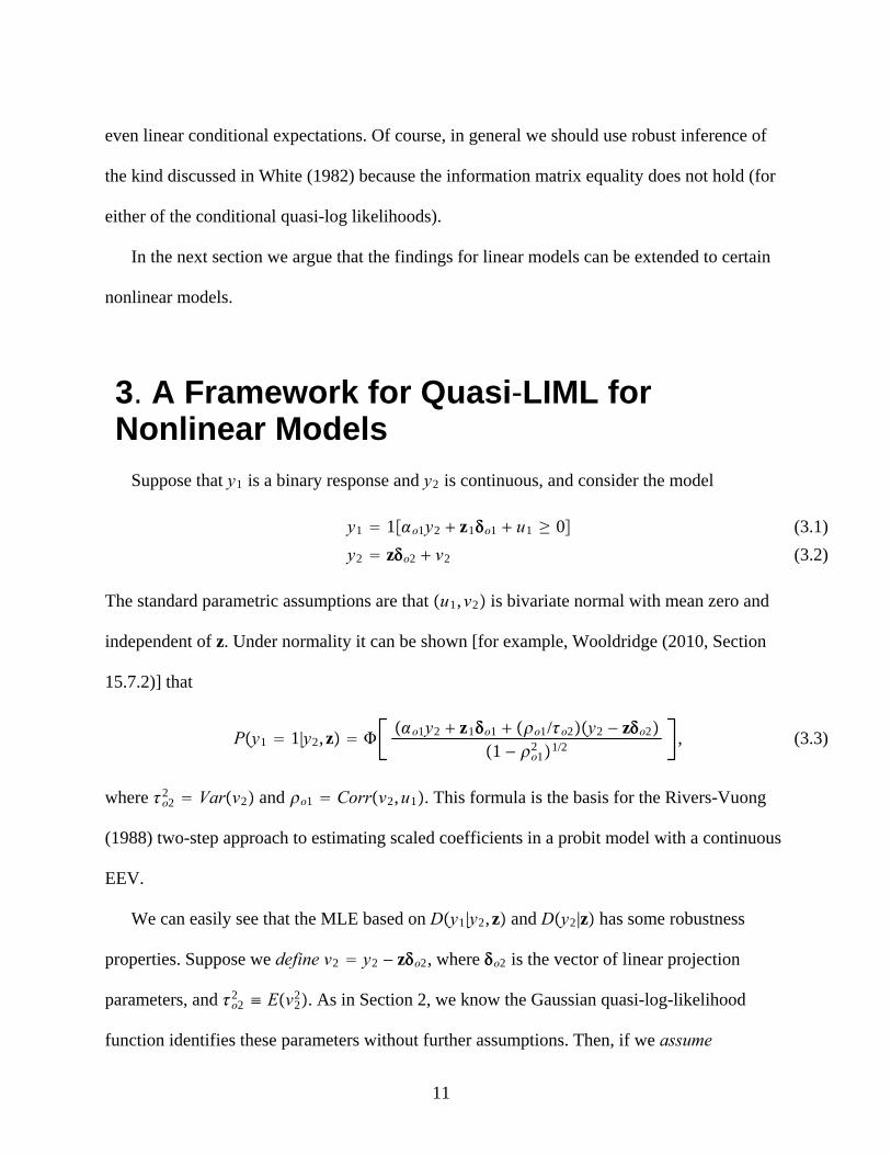
even linear conditional expectations. Of course, in general we should use robust inference of
the kind discussed in White (1982) because the information matrix equality does not hold (for
either of the conditional quasi-log likelihoods).
In the next section we argue that the findings for linear models can be extended to certain
nonlinear models.
3. A Framework for Quasi-LIML forNonlinear Models
Suppose that y1 is a binary response and y2 is continuous, and consider the model
y1 1o1y2 z1o1 u1 ≥ 0
y2 zo2 v2
(3.1)
(3.2)
The standard parametric assumptions are that u1,v2 is bivariate normal with mean zero and
independent of z. Under normality it can be shown [for example, Wooldridge (2010, Section
15.7.2)] that
Py1 1|y2,z o1y2 z1o1 o1/o2y2 − zo21 − o12 1/2
, (3.3)
where o22 Varv2 and o1 Corrv2,u1. This formula is the basis for the Rivers-Vuong
(1988) two-step approach to estimating scaled coefficients in a probit model with a continuous
EEV.
We can easily see that the MLE based on Dy1|y2,z and Dy2|z has some robustness
properties. Suppose we define v2 y2 − zo2, where o2 is the vector of linear projection
parameters, and o22 ≡ Ev22. As in Section 2, we know the Gaussian quasi-log-likelihood
function identifies these parameters without further assumptions. Then, if we assume
11
Page 12
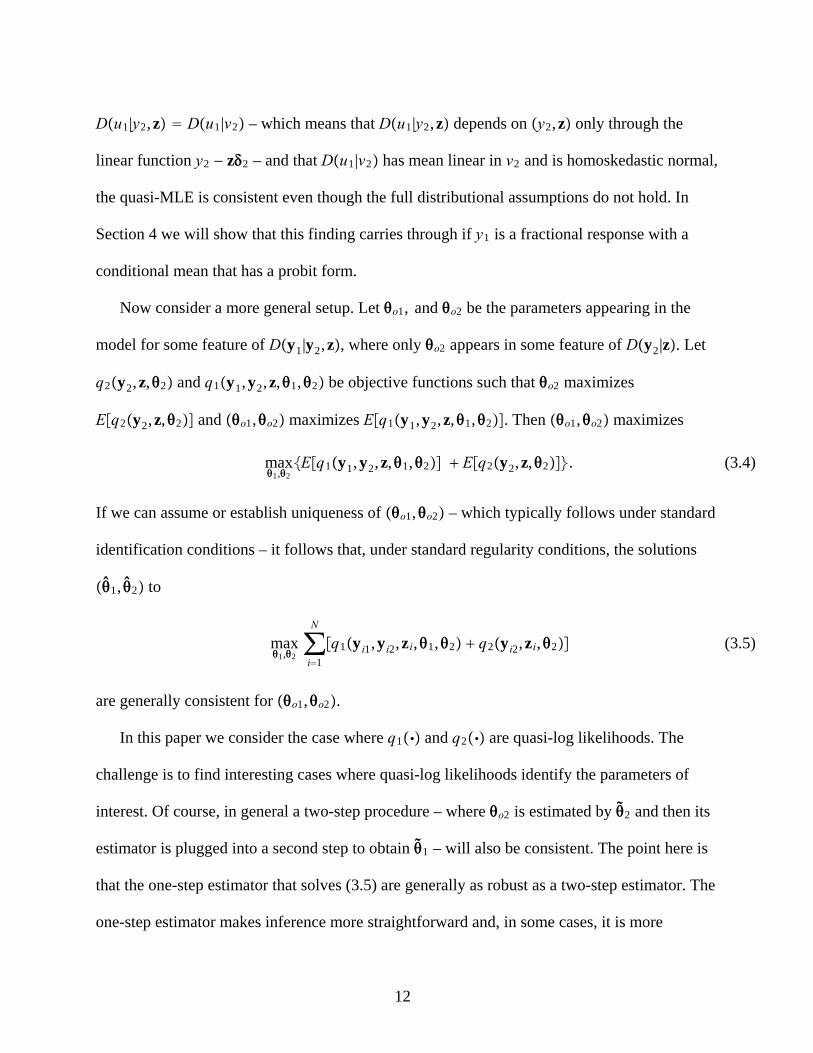
Du1|y2,z Du1|v2 – which means that Du1|y2,z depends on y2,z only through the
linear function y2 − z2 – and that Du1|v2 has mean linear in v2 and is homoskedastic normal,
the quasi-MLE is consistent even though the full distributional assumptions do not hold. In
Section 4 we will show that this finding carries through if y1 is a fractional response with a
conditional mean that has a probit form.
Now consider a more general setup. Let o1, and o2 be the parameters appearing in the
model for some feature of Dy1|y2,z, where only o2 appears in some feature of Dy2|z. Let
q2y2,z,2 and q1y1,y2,z,1,2 be objective functions such that o2 maximizes
Eq2y2,z,2 and o1,o2 maximizes Eq1y1,y2,z,1,2. Then o1,o2 maximizes
max1,2
Eq1y1,y2,z,1,2 Eq2y2,z,2. (3.4)
If we can assume or establish uniqueness of o1,o2 – which typically follows under standard
identification conditions – it follows that, under standard regularity conditions, the solutions
1, 2 to
max1,2∑i1
N
q1yi1,yi2,zi,1,2 q2yi2,zi,2 (3.5)
are generally consistent for o1,o2.
In this paper we consider the case where q1 and q2 are quasi-log likelihoods. The
challenge is to find interesting cases where quasi-log likelihoods identify the parameters of
interest. Of course, in general a two-step procedure – where o2 is estimated by 2 and then its
estimator is plugged into a second step to obtain 1 – will also be consistent. The point here is
that the one-step estimator that solves (3.5) are generally as robust as a two-step estimator. The
one-step estimator makes inference more straightforward and, in some cases, it is more
12
Page 13
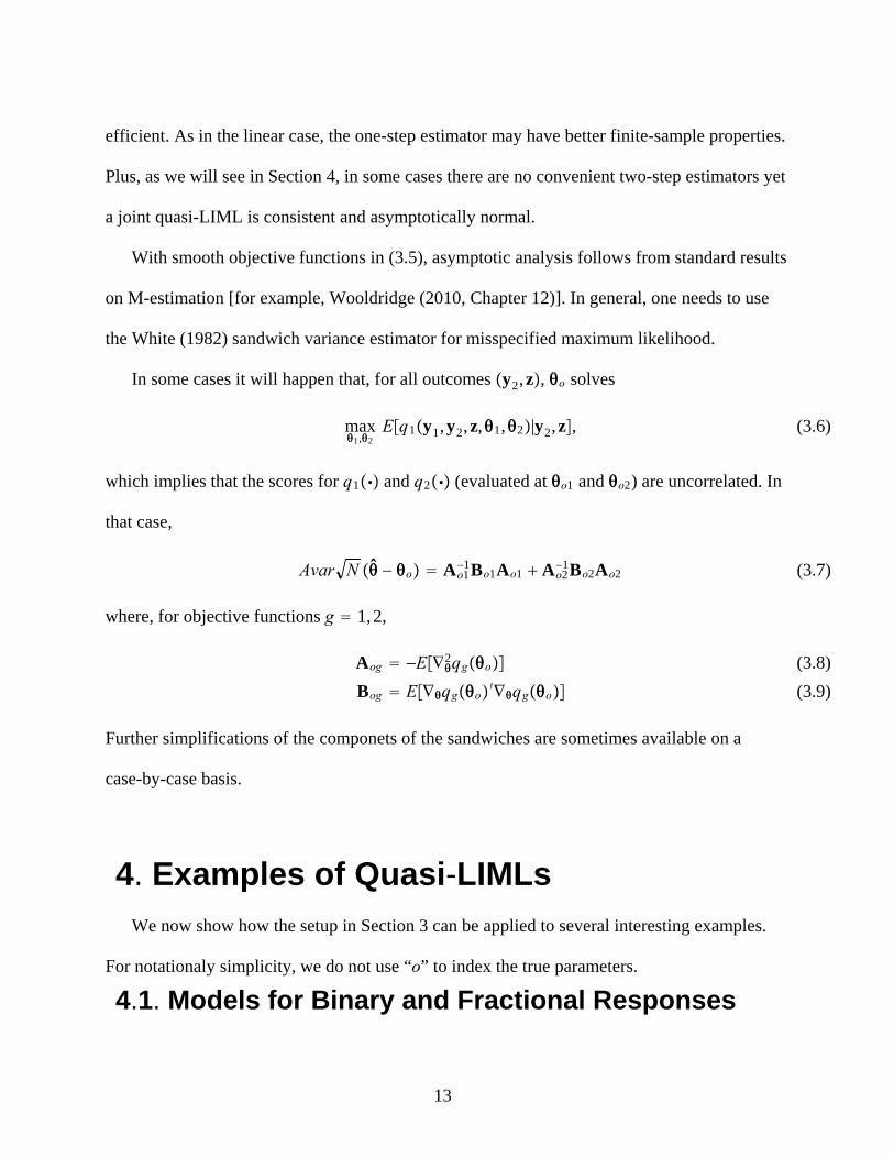
efficient. As in the linear case, the one-step estimator may have better finite-sample properties.
Plus, as we will see in Section 4, in some cases there are no convenient two-step estimators yet
a joint quasi-LIML is consistent and asymptotically normal.
With smooth objective functions in (3.5), asymptotic analysis follows from standard results
on M-estimation [for example, Wooldridge (2010, Chapter 12)]. In general, one needs to use
the White (1982) sandwich variance estimator for misspecified maximum likelihood.
In some cases it will happen that, for all outcomes y2,z, o solves
max1,2
Eq1y1,y2,z,1,2|y2,z, (3.6)
which implies that the scores for q1 and q2 (evaluated at o1 and o2) are uncorrelated. In
that case,
Avar N − o Ao1−1Bo1Ao1 Ao2
−1Bo2Ao2 (3.7)
where, for objective functions g 1,2,
Aog −E∇2qgo
Bog E∇qgo ′∇qgo
(3.8)
(3.9)
Further simplifications of the componets of the sandwiches are sometimes available on a
case-by-case basis.
4. Examples of Quasi-LIMLs
We now show how the setup in Section 3 can be applied to several interesting examples.
For notationaly simplicity, we do not use “o” to index the true parameters.
4.1. Models for Binary and Fractional Responses
13
Page 14
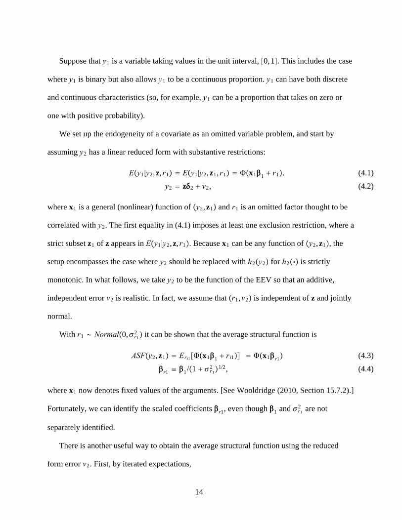
Suppose that y1 is a variable taking values in the unit interval, 0,1. This includes the case
where y1 is binary but also allows y1 to be a continuous proportion. y1 can have both discrete
and continuous characteristics (so, for example, y1 can be a proportion that takes on zero or
one with positive probability).
We set up the endogeneity of a covariate as an omitted variable problem, and start by
assuming y2 has a linear reduced form with substantive restrictions:
Ey1|y2,z, r1 Ey1|y2,z1, r1 x11 r1.
y2 z2 v2,
(4.1)
(4.2)
where x1 is a general (nonlinear) function of y2,z1 and r1 is an omitted factor thought to be
correlated with y2. The first equality in (4.1) imposes at least one exclusion restriction, where a
strict subset z1 of z appears in Ey1|y2,z, r1. Because x1 can be any function of y2,z1, the
setup encompasses the case where y2 should be replaced with h2y2 for h2 is strictly
monotonic. In what follows, we take y2 to be the function of the EEV so that an additive,
independent error v2 is realistic. In fact, we assume that r1,v2 is independent of z and jointly
normal.
With r1 Normal0,r12 it can be shown that the average structural function is
ASFy2,z1 Eri1x11 ri1 x1r1
r1 ≡ 1/1 r12 1/2,
(4.3)
(4.4)
where x1 now denotes fixed values of the arguments. [See Wooldridge (2010, Section 15.7.2).]
Fortunately, we can identify the scaled coefficients r1, even though 1 and r12 are not
separately identified.
There is another useful way to obtain the average structural function using the reduced
form error v2. First, by iterated expectations,
14
Page 15
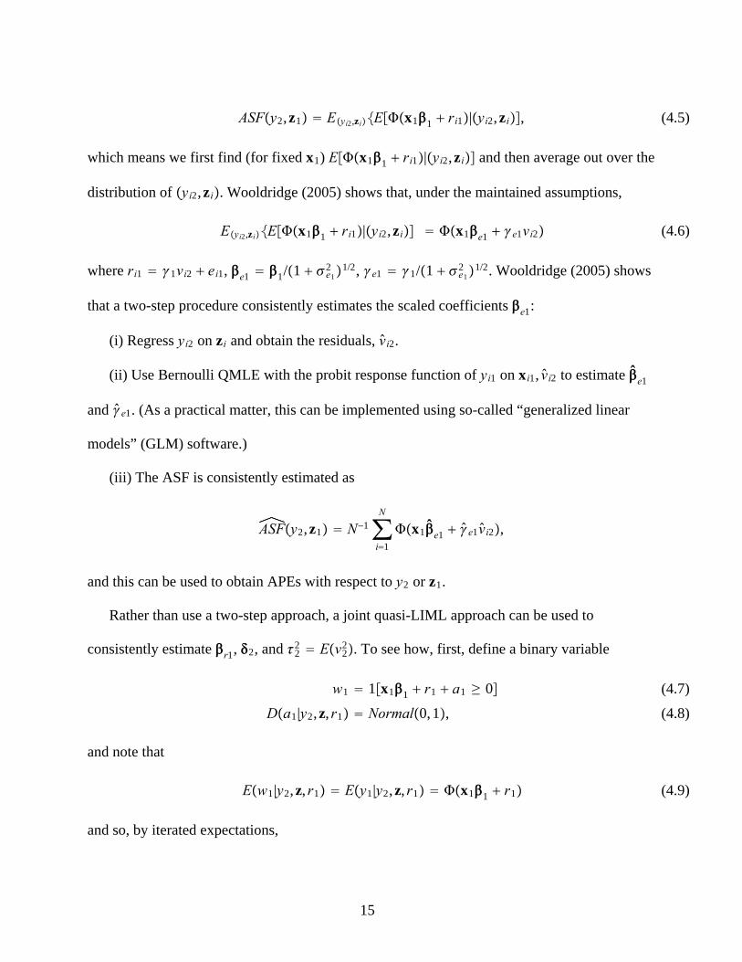
ASFy2,z1 Eyi2,ziEx11 ri1|yi2,zi, (4.5)
which means we first find (for fixed x1) Ex11 ri1|yi2,zi and then average out over the
distribution of yi2,zi. Wooldridge (2005) shows that, under the maintained assumptions,
Eyi2,ziEx11 ri1|yi2,zi x1e1 e1vi2 (4.6)
where ri1 1vi2 ei1, e1 1/1 e12 1/2, e1 1/1 e1
2 1/2. Wooldridge (2005) shows
that a two-step procedure consistently estimates the scaled coefficients e1:
(i) Regress yi2 on zi and obtain the residuals, vi2.
(ii) Use Bernoulli QMLE with the probit response function of yi1 on xi1, vi2 to estimate e1
and e1. (As a practical matter, this can be implemented using so-called “generalized linear
models” (GLM) software.)
(iii) The ASF is consistently estimated as
ASFy2,z1 N−1∑i1
N
x1e1 e1vi2,
and this can be used to obtain APEs with respect to y2 or z1.
Rather than use a two-step approach, a joint quasi-LIML approach can be used to
consistently estimate r1, 2, and 22 Ev2
2. To see how, first, define a binary variable
w1 1x11 r1 a1 ≥ 0
Da1|y2,z, r1 Normal0,1,
(4.7)
(4.8)
and note that
Ew1|y2,z, r1 Ey1|y2,z, r1 x11 r1 (4.9)
and so, by iterated expectations,
15
Page 16
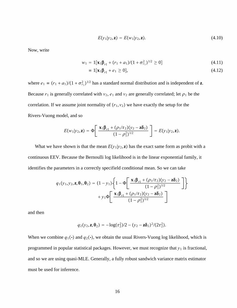
Ey1|y2,z Ew1|y2,z. (4.10)
Now, write
w1 1x1r1 r1 a1/1 r12 1/2 ≥ 0
≡ 1x1r1 e1 ≥ 0,
(4.11)
(4.12)
where e1 ≡ r1 a1/1 r12 1/2 has a standard normal distribution and is independent of z.
Because r1 is generally correlated with v2, e1 and v2 are generally correlated; let 1 be the
correlation. If we assume joint normality of r1,v2 we have exactly the setup for the
Rivers-Vuong model, and so
Ew1|y2,z x1r1 1/2y2 − z2
1 − 121/2
Ey1|y2,z.
What we have shown is that the mean Ey1|y2,z has the exact same form as probit with a
continuous EEV. Because the Bernoulli log likelihood is in the linear exponential family, it
identifies the parameters in a correctly specifield conditional mean. So we can take
q1y1,y2,z,1,2 1 − y1 1 − x1r1 1/2y2 − z2
1 − 121/2
y1x1r1 1/2y2 − z2
1 − 121/2
and then
q2y2,z,2 − log22/2 − y2 − z22/22
2.
When we combine q1 and q2, we obtain the usual Rivers-Vuong log likelihood, which is
programmed in popular statistical packages. However, we must recognize that y1 is fractional,
and so we are using quasi-MLE. Generally, a fully robust sandwich variance matrix estimator
must be used for inference.
16
Page 17
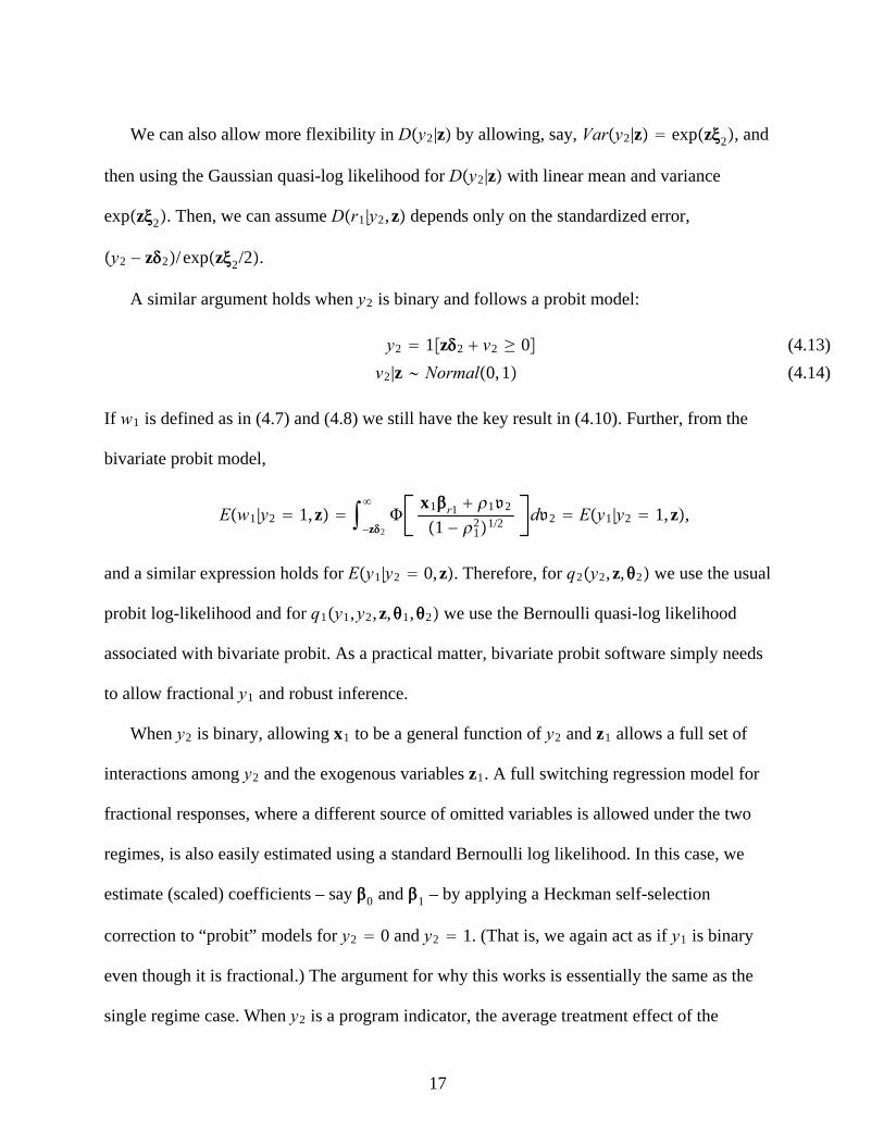
We can also allow more flexibility in Dy2|z by allowing, say, Vary2|z expz2, and
then using the Gaussian quasi-log likelihood for Dy2|z with linear mean and variance
expz2. Then, we can assume Dr1|y2,z depends only on the standardized error,
y2 − z2/ expz2/2.
A similar argument holds when y2 is binary and follows a probit model:
y2 1z2 v2 ≥ 0
v2|z Normal0,1
(4.13)
(4.14)
If w1 is defined as in (4.7) and (4.8) we still have the key result in (4.10). Further, from the
bivariate probit model,
Ew1|y2 1,z −z2
x1r1 1v2
1 − 121/2
dv2 Ey1|y2 1,z,
and a similar expression holds for Ey1|y2 0,z. Therefore, for q2y2,z,2 we use the usual
probit log-likelihood and for q1y1,y2,z,1,2 we use the Bernoulli quasi-log likelihood
associated with bivariate probit. As a practical matter, bivariate probit software simply needs
to allow fractional y1 and robust inference.
When y2 is binary, allowing x1 to be a general function of y2 and z1 allows a full set of
interactions among y2 and the exogenous variables z1. A full switching regression model for
fractional responses, where a different source of omitted variables is allowed under the two
regimes, is also easily estimated using a standard Bernoulli log likelihood. In this case, we
estimate (scaled) coefficients – say 0 and 1 – by applying a Heckman self-selection
correction to “probit” models for y2 0 and y2 1. (That is, we again act as if y1 is binary
even though it is fractional.) The argument for why this works is essentially the same as the
single regime case. When y2 is a program indicator, the average treatment effect of the
17
Page 18
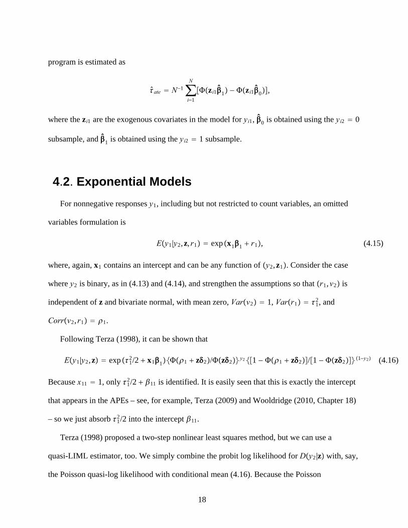
program is estimated as
ate N−1∑i1
N
zi11 − zi10,
where the zi1 are the exogenous covariates in the model for yi1, 0 is obtained using the yi2 0
subsample, and 1 is obtained using the yi2 1 subsample.
4.2. Exponential Models
For nonnegative responses y1, including but not restricted to count variables, an omitted
variables formulation is
Ey1|y2,z, r1 exp x11 r1, (4.15)
where, again, x1 contains an intercept and can be any function of y2,z1. Consider the case
where y2 is binary, as in (4.13) and (4.14), and strengthen the assumptions so that r1,v2 is
independent of z and bivariate normal, with mean zero, Varv2 1, Varr1 12, and
Corrv2, r1 1.
Following Terza (1998), it can be shown that
Ey1|y2,z exp 12/2 x111 z2/z2y21 − 1 z2/1 − z21−y2 (4.16)
Because x11 1, only 12/2 11 is identified. It is easily seen that this is exactly the intercept
that appears in the APEs – see, for example, Terza (2009) and Wooldridge (2010, Chapter 18)
– so we just absorb 12/2 into the intercept 11.
Terza (1998) proposed a two-step nonlinear least squares method, but we can use a
quasi-LIML estimator, too. We simply combine the probit log likelihood for Dy2|z with, say,
the Poisson quasi-log likelihood with conditional mean (4.16). Because the Poisson
18
Page 19
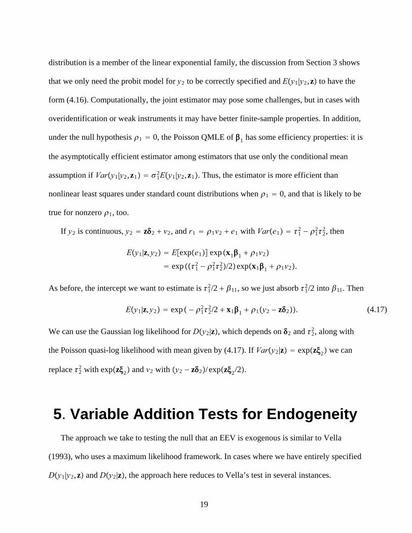
distribution is a member of the linear exponential family, the discussion from Section 3 shows
that we only need the probit model for y2 to be correctly specified and Ey1|y2,z to have the
form (4.16). Computationally, the joint estimator may pose some challenges, but in cases with
overidentification or weak instruments it may have better finite-sample properties. In addition,
under the null hypothesis 1 0, the Poisson QMLE of 1 has some efficiency properties: it is
the asymptotically efficient estimator among estimators that use only the conditional mean
assumption if Vary1|y2,z1 12Ey1|y2,z1. Thus, the estimator is more efficient than
nonlinear least squares under standard count distributions when 1 0, and that is likely to be
true for nonzero 1, too.
If y2 is continuous, y2 z2 v2, and r1 1v2 e1 with Vare1 12 − 1
222, then
Ey1|z,y2 Eexpe1 exp x11 1v2
exp 12 − 1
222/2expx11 1v2.
As before, the intercept we want to estimate is 12/2 11, so we just absorb 1
2/2 into 11. Then
Ey1|z,y2 exp − 122
2/2 x11 1y2 − z2. (4.17)
We can use the Gaussian log likelihood for Dy2|z, which depends on 2 and 22, along with
the Poisson quasi-log likelihood with mean given by (4.17). If Vary2|z expz2 we can
replace 22 with expz2 and v2 with y2 − z2/ expz2/2.
5. Variable Addition Tests for Endogeneity
The approach we take to testing the null that an EEV is exogenous is similar to Vella
(1993), who uses a maximum likelihood framework. In cases where we have entirely specified
Dy1|y2,z and Dy2|z, the approach here reduces to Vella’s test in several instances.
19
Page 20
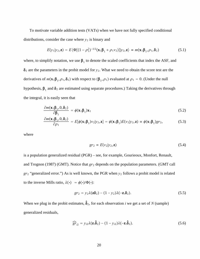
To motivate variable addition tests (VATs) when we have not fully specified conditional
distributions, consider the case where y2 is binary and
Ey1|y2,z E1 − 12−1/2x11 1v2|y2,z ≡ mx11,1,2 (5.1)
where, to simplify notation, we use 1 to denote the scaled coefficients that index the ASF, and
2 are the parameters in the probit model for y2. What we need to obtain the score test are the
derivatives of mx11,1,2 with respect to 1,1 evaluated at 1 0. (Under the null
hypothesis, 1 and 2 are estimated using separate procedures.) Taking the derivatives through
the integral, it is easily seen that
∂mx11, 0,2∂1
x11x1
∂mx11, 0,2∂1
Ex11v2|y2,z x11Ev2|y2,z ≡ x11gr2,
(5.2)
(5.3)
where
gr2 ≡ Ev2|y2,z (5.4)
is a population generalized residual (PGR) – see, for example, Gourieoux, Monfort, Renault,
and Trognon (1987) (GMT). Notice that gr2 depends on the population parameters. (GMT call
gr2 “generalized error.”) As is well known, the PGR when y2 follows a probit model is related
to the inverse Mills ratio, /:
gr2 y2z2 − 1 − y2−zi2. (5.5)
When we plug in the probit estimates, 2, for each observation i we get a set of N (sample)
generalized residuals,
gri2 yi2zi2 − 1 − yi2−zi2. (5.6)
20
Page 21
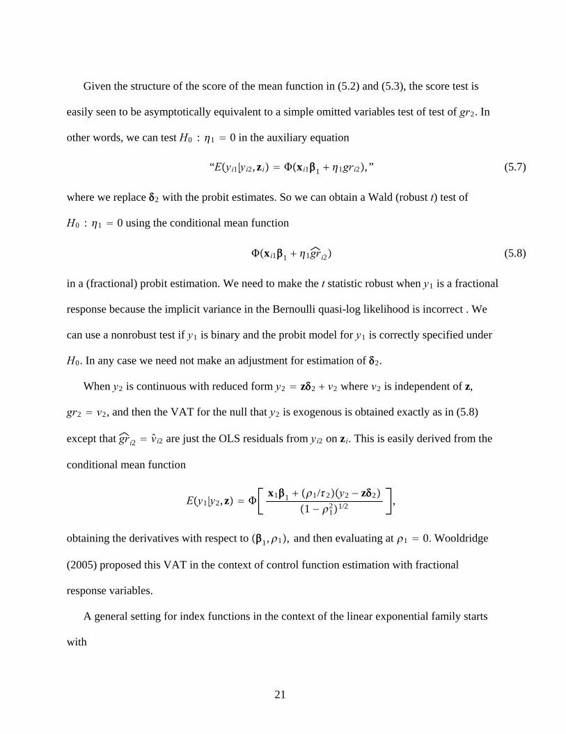
Given the structure of the score of the mean function in (5.2) and (5.3), the score test is
easily seen to be asymptotically equivalent to a simple omitted variables test of test of gr2. In
other words, we can test H0 : 1 0 in the auxiliary equation
“Eyi1|yi2,zi xi11 1gri2, ” (5.7)
where we replace 2 with the probit estimates. So we can obtain a Wald (robust t) test of
H0 : 1 0 using the conditional mean function
xi11 1gri2 (5.8)
in a (fractional) probit estimation. We need to make the t statistic robust when y1 is a fractional
response because the implicit variance in the Bernoulli quasi-log likelihood is incorrect . We
can use a nonrobust test if y1 is binary and the probit model for y1 is correctly specified under
H0. In any case we need not make an adjustment for estimation of 2.
When y2 is continuous with reduced form y2 z2 v2 where v2 is independent of z,
gr2 v2, and then the VAT for the null that y2 is exogenous is obtained exactly as in (5.8)
except that gri2 vi2 are just the OLS residuals from yi2 on zi. This is easily derived from the
conditional mean function
Ey1|y2,z x11 1/2y2 − z2
1 − 121/2
,
obtaining the derivatives with respect to 1,1, and then evaluating at 1 0. Wooldridge
(2005) proposed this VAT in the context of control function estimation with fractional
response variables.
A general setting for index functions in the context of the linear exponential family starts
with
21
Page 22
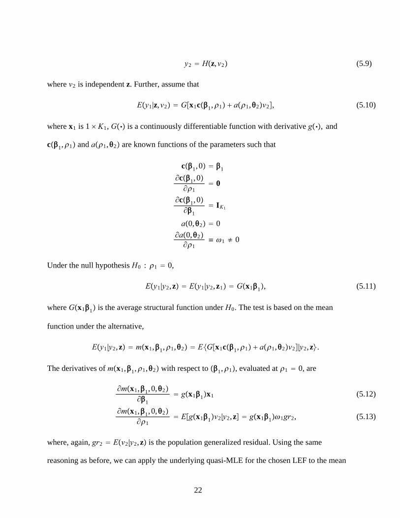
y2 Hz,v2 (5.9)
where v2 is independent z. Further, assume that
Ey1|z,v2 Gx1c1,1 a1,2v2, (5.10)
where x1 is 1 K1, G is a continuously differentiable function with derivative g, and
c1,1 and a1,2 are known functions of the parameters such that
c1, 0 1
∂c1, 0∂1
0
∂c1, 0∂1
IK1
a0,2 0
∂a0,2∂1
≡ 1 ≠ 0
Under the null hypothesis H0 : 1 0,
Ey1|y2,z Ey1|y2,z1 Gx11, (5.11)
where Gx11 is the average structural function under H0. The test is based on the mean
function under the alternative,
Ey1|y2,z mx1,1,1,2 EGx1c1,1 a1,2v2|y2,z.
The derivatives of mx1,1,1,2 with respect to 1,1, evaluated at 1 0, are
∂mx1,1, 0,2∂1
gx11x1
∂mx1,1, 0,2∂1
Egx11v2|y2,z gx111gr2,
(5.12)
(5.13)
where, again, gr2 Ev2|y2,z is the population generalized residual. Using the same
reasoning as before, we can apply the underlying quasi-MLE for the chosen LEF to the mean
22
Page 23
function
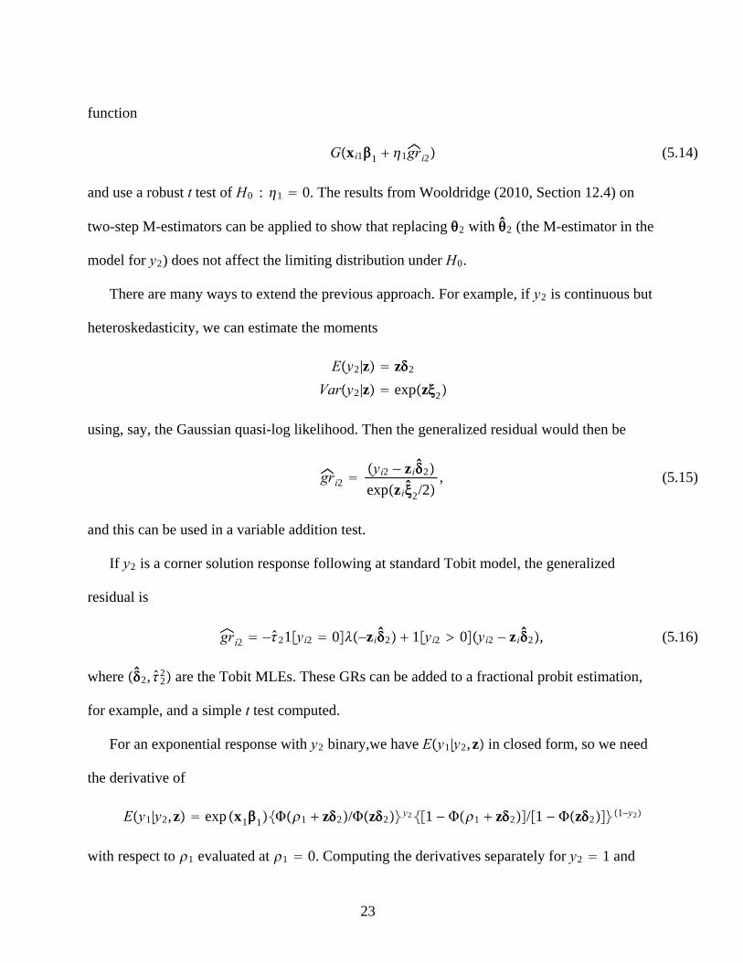
Gxi11 1gri2 (5.14)
and use a robust t test of H0 : 1 0. The results from Wooldridge (2010, Section 12.4) on
two-step M-estimators can be applied to show that replacing 2 with 2 (the M-estimator in the
model for y2) does not affect the limiting distribution under H0.
There are many ways to extend the previous approach. For example, if y2 is continuous but
heteroskedasticity, we can estimate the moments
Ey2|z z2
Vary2|z expz2
using, say, the Gaussian quasi-log likelihood. Then the generalized residual would then be
gri2 yi2 − zi2expzi2/2
, (5.15)
and this can be used in a variable addition test.
If y2 is a corner solution response following at standard Tobit model, the generalized
residual is
gri2 −21yi2 0−zi2 1yi2 0yi2 − zi2, (5.16)
where 2, 22 are the Tobit MLEs. These GRs can be added to a fractional probit estimation,
for example, and a simple t test computed.
For an exponential response with y2 binary,we have Ey1|y2,z in closed form, so we need
the derivative of
Ey1|y2,z exp x111 z2/z2y21 − 1 z2/1 − z21−y2
with respect to 1 evaluated at 1 0. Computing the derivatives separately for y2 1 and
23
Page 24
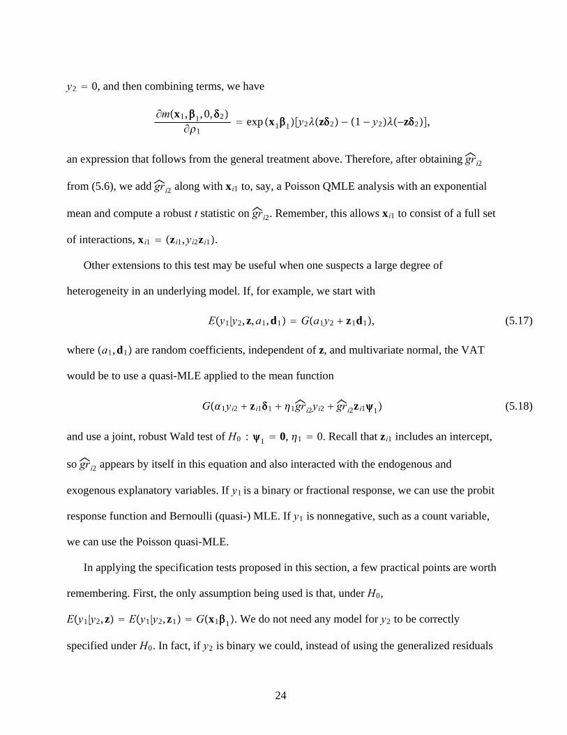
y2 0, and then combining terms, we have
∂mx1,1, 0,2∂1
exp x11y2z2 − 1 − y2−z2,
an expression that follows from the general treatment above. Therefore, after obtaining gri2
from (5.6), we add gri2 along with xi1 to, say, a Poisson QMLE analysis with an exponential
mean and compute a robust t statistic on gri2. Remember, this allows xi1 to consist of a full set
of interactions, xi1 zi1,yi2zi1.
Other extensions to this test may be useful when one suspects a large degree of
heterogeneity in an underlying model. If, for example, we start with
Ey1|y2,z,a1,d1 Ga1y2 z1d1, (5.17)
where a1,d1 are random coefficients, independent of z, and multivariate normal, the VAT
would be to use a quasi-MLE applied to the mean function
G1yi2 zi11 1gri2yi2 gri2zi11 (5.18)
and use a joint, robust Wald test of H0 : 1 0, 1 0. Recall that zi1 includes an intercept,
so gri2 appears by itself in this equation and also interacted with the endogenous and
exogenous explanatory variables. If y1 is a binary or fractional response, we can use the probit
response function and Bernoulli (quasi-) MLE. If y1 is nonnegative, such as a count variable,
we can use the Poisson quasi-MLE.
In applying the specification tests proposed in this section, a few practical points are worth
remembering. First, the only assumption being used is that, under H0,
Ey1|y2,z Ey1|y2,z1 Gx11. We do not need any model for y2 to be correctly
specified under H0. In fact, if y2 is binary we could, instead of using the generalized residuals
24
Page 25
obtained from probit, use the OLS residuals obtained from a linear probability model and still
obtain a valid test under the null. The reason for preferring a test based on the GRs is that the
test is optimal (has highest local asymptotic power) under correct specification of the probit
model for y2. Second, as in any specification testing context, a rejection of the null may occur
for many reasons. The variable y2 may be endogenous, but it could also be that the conditional
mean Ey1|y2,z1 is misspecified. Third, by following the approach proposed in this section,
the tests will not reject due to misspecifications of Dy1|y2,z other than Ey1|y2,z1. Thus, the
tests are robust because no auxiliary assumptions are imposed under the null.
6. A General Control Function Approach
The setup in Section 3, illustrated in Section 4, allows for joint and one-step QMLE in a
variety of situations, but these methods can be difficult to apply with certain discrete response
models for y1 or discrete EEVs, or both, particularly if we have more than one EEV. Even
slight extensions of standard models are difficult to handle if we are wedded to starting with a
“structural” model for y1 and then trying to obtain full MLEs or two-step estimators.
As an example, consider a probit response function with a binary EEV, but were the latter
interacts with unobserved heterogeneity:
Ey1|y2,z1,a1,d1 a1y2 z1d1
1y2 z11 c1y2 z1q1
y2 1z2 v2 0
(6.1)
(6.2)
(6.3)
where a1 1 c1 and d1 1 q1. Now, if a1,q1,v2 is multivariate normal we could use
a joint QMLE by finding Ey1|y2,z. But the expectation is not in closed form and the resulting
procedure would be computationally intensive.
25
Page 26
An alternative approach is suggested by the VATs derived in Section 5 combined with the
insights of Blundell and Powell (2003, 2004) and Wooldridge (2005). To describe the
approach, we need to review Blundell and Powell (2004) and the slight extension due to
Wooldridge (2005). BP study a fully nonparametric situation where
y1 g1y2,z1,u1 (6.4)
for unobservables u1. The average structural function is
ASFy2,z1 ≡ Eui1g1y2,z1,ui1, (6.5)
so that the unobservables are averaged out. Further, BP assume that y2 (a scalar here for
simplicity) has the representation
y2 g2z v2, (6.6)
where u1,v2 is independent of z. Under independence of u1,v2 and the representation
y2 g2z v2,
Du1|y2,z Du1|v2. (6.7)
Further, as shown by BP (2004), the ASF can be obtained from
h1y2,z1,v2 ≡ Ey1|y2,z1,v2. (6.8)
In particular,
ASFy2,z1 Evi2h1y2,z1,vi2.
Unlike the ui1, for identification purposes we effectively observe the vi2 because
vi2 yi2 − g2zi, and g2 is nonparametrically identified. (Of course, we can also model
g2 parametrically and use standard N -asymptotically normal estimators.) Letting
vi2 yi2 − ĝ2zi (6.9)
26
Page 27
denote the reduced form residuals, a consistent estimator of the ASF, under weak regularity
conditions, is
ASFy2,z1 N−1∑i1
N
ĥ1y2,z1, vi2. (6.10)
The BP (2004) framework is very general when it comes to allowing flexibility in g1 and
g2; in effect, an exclusion restriction is needed in the former and the latter must depend on
at least one excluded exogenous variable. Even if one wants to stay within a parametric
framework, the BP approach is liberating because it shows that a quantity of considerable
interest – the ASF – can be obtained from Ey1|y2,z1,v2 without worrying about the structural
function g1. In a parametric setting this means that, once Ey2|z is modeled and estimated,
attention can turn to Ey1|y2,z1,v2 or possibly Dy1|y2,z1,v2.
Directly modeling Dy1|y2,z1,v2 is the approach taken by Petrin and Train (2010) when y1
is a multinomial response (product choice) and y2 is replaced with a vector of prices. Starting
with standard models for Dy1|y2,z1,u1 – such as multinomial logit or nested logit – where u1
includes heterogeneous tastes, leads to complicated estimators. Petrin and Train suggest
modeling Dy1|y2,z1,v2 directly, where v2 is a vector of reduced form errors:
y2 G2z v2. Given a linear reduced form for y2, the two-step estimation method is very
simple, because the second step is multinomial logit, nested logit, or a mixed logit model.
When the EEVs are continuous, approaches such as that proposed by Petrin and Train
(2010) can be viewed as convenient parametric approximations to an analysis that could be
made fully nonparametric (subject to practical issues such as number of observations relative
to the dimension of the explanatory variables). Unfortunately, when y2 is discrete, standard
models for Dy2|z along with structural models for Dy1|y2,z,u1, do not generally lead to
27
Page 28
simple CF estimation. Moreover, models with discrete EEVs are generally nonparametrically
identified (for example, Chesher, 2003). Therefore, if we want point estimates of average
partial effects when y2 is discrete, we must rely on parametric assumptions.
As we saw in Section 4, for a wide class of nonlinear models adding the generalized
residual produces a test for the null that y2 is exogenous. What if, as a general strategy, we use
generalized residuals as control functions in parametric nonlinear models with the hope that
this (largely) solves the endogeneity problem?
It is useful to determine assumptions under which a two-step control function method can
produce consistent estimators when the EEVs are discrete. For simplicity take y2 to be a scalar,
and first assume
Ey1|y2,z,r1 Ey1|y2,z1,r1, (6.11)
which imposes the exclusion restriction conditional on heterogeneity r1. Notice that this
condition generalizes the BP approach because it allows for additional unobservables without
taking a stand on the exact nature of those unobservables – they could have discreteness, for
example. This extension is important for handling models such as fractional responses or
nonnegative responses because it is more natural to specify, say,
Ey1|y2,z1, r1 1y2 z11 r1 then to write y1 as a deterministic function of a larger
set of unobservables.
Next, let e2 k2y2,z be the proposed control function for some function k2. Under
(6.11),
Ey1|y2,z1,r1,e2 Ey1|y2,z1,r1,
so that e2 is properly excluded from the structural conditional expectation. Further, a key
28
Page 29
restriction, following BP and Wooldridge (2005), is
Dr1|y2,z Dr1|e2. (6.12)
In other words, e2 acts as a kind of sufficient statistic for characterizing the endogeneity of y2.
In the BP setup, e2 ≡ v2 y2 − g2z. In the Heckman linear switching regression framework,
e2 gr2 suffices, where gr2 is the generalized residual.
In general, we can verify (6.12) by starting with a generalization of the BP setup by
relaxing additivity of v2:
y2 g2z,v2 (6.13)
Then, we assume two conditions that imply (6.12):
Dr1|z,v2 Dr1|v2
Dv2|y2,z Dv2|e2
(6.14)
(6.15)
Condition (6.14) is standard, as it is implied by r1,v2 independent of z. Condition (6.15) can
be shown in some cases where e2 includes generalized residuals – as in the binary response
case, for example.
If we maintain (6.11) and (6.12) then it follows from Wooldridge (2010, Section 2.2.5) that
the ASF can be obtained as
ASFy2,z1 Eei2h2y2,z1,ei2, (6.16)
where
h2y2,z1,e2 Ey1|y2,z1,e2. (6.17)
Asserting that (6.12) holds for discrete y2 has precedence, although it is typically imposed
indirectly. For example, Terza, Basu, and Rathouz (2008) (TBR) effectively use this
assumption when e2 y2 − z2, where y2 is binary and follows a probit model. In fact, for
29
Page 30
binary y1, TBR suppose a parametric model,
y1 11y2 z11 u1 0
u1 1e2 a1
a1|y2,z Normal0,12
[Burnett (1997) actually proposed this approach but without any justification.] Given that the
score test uses the generalized residual, and that Eu1|y2,z is linear in the generalized residual
(not e2 y2 − z2), it seems slightly preferred to use the generalized residuals as e2. It is
important to remember that neither can be justified using the usual assumptions for the
bivariate probit model and neither is more or less general than the usual bivariate probit
assumptions.
Generally, my suggestion is to use convenient parametric models maintaining the key
condition (6.12) for an appropriately chosen function e2, typically a generalized residual. Then
parametric models can be applied to estimate the conditional mean Ey1|y2,z1,e2. In some
cases, we may actually specify a full conditional distribution, Dy1|y2,z1,e2 for example, if y1
is a binary, multinomial, or ordered response. The general method is as follows, assuming a
random sample of size N from the population:
1. Estimate a model for Dy2|z [or sometimes only for Ey2|z], where the model depends
on parameters 2. For the function ei2 k2yi2,zi,2, define generalized residuals as
êi2 k2yi2,zi, 2. (6.18)
2. Estimate a parametric model for Ey1|y2,z1,e2 using a quasi-MLE by inserting êi2 for
ei2. Or, if Dy1|y2,z1,e2 has been fully specified, use MLE. In either case, let the parameter
estimator be 1.
3. Estimate the ASF as
30
Page 31
ASFy2,z1 N−1∑i1
N
h1y2,z1,êi2, 1 (6.19)
where h1y2,z1,e2,1 Ey1|y2,z1,e2.
Inference concerning ASF can be obtained using the delta method – the particular form is
described in Wooldridge (2010, Problem 12.17) – or bootstrapping the two estimation steps.
How might we apply the general CF approach to the problem described in equations (6.1),
(6.2), and (6.3)? First, we would not specify (6.1) as the structural conditional mean, but we
would assume that (6.12) holds for e2 gr2 and use a mean function such as
Eyi1|yi2,zi1,gri2 1yi2 zi11 1gri2 yi2 gri2 zi11. (6.20)
In other words, we take a standard functional form that restricts the mean function to the unit
interval – in this case the probit function – and add the control function in a fairly flexible way.
We get a simple test for the null of exogeneity and, hopefully, a reasonable approximation to
the ASF when we average out gri2:
ASFy2,z1 N−1∑i1
N
1y2 z11 1gri2 y2 gri2 z11. (6.21)
A similar strategy is available if y2 is a corner solution and follows a Tobit model. In this case,
the generalized residual is given in equation (5.16).
An approach based on (6.20) is neither more nor less general than an approach that starts
by specifying Dy1|y2,z1,u1 and parametric assumptions in (6.13). While a more structural
approach may have more appeal conceptually, it is not nearly as simple as the control function
approach based on (6.20). If we are interested in the average structural function, (6.20) is more
direct.
31
Page 32
The drawback to the CF approach – one that it shares with structural approaches – is that it
relies on parametric functional forms. Because the ASF is not parametrically identified when
y2 is discrete, we have few options. Either we can use a parametric structural approach – an
example is given in Section 4.1 – the CF approach, change the quantity of interest, or only try
to bound specific parameters (such as an average treatment effect). The CF approach proposed
here should be viewed as a computationally simple complement to other approaches.
7. Concluding Remarks
I have argued that a general quasi-LIML approach can be used to obtain one-step estimator
for nonlinear models with endogenous explanatory variables. This approach leads to estimators
that are new for certain kinds of response variables, including a fractional response with a
binary endogenous explanatory variable. There are both theoretical and practical issues left to
be resolved. For example, in a quasi-MLE framework, are there useful conditions under which
the one-step quasi-LIML is asymptotically more efficient than a two-step control function
approach? Also, in a nonlinear setting, when might the one-step estimator have less bias than a
two-step method (provided there is a consistent two-step estimator available)?
The variable addition tests can be applied in a variety of settings when a generalized
residual for the EEV can be computed. These tests are computationally very simple. One issue
that needs further study is the best way to obtain tests when y2 is a vector of EEVs, some of
which are discrete.
The CF framework for discrete EEVs proposed in Section 6 can be justified under
parametric assumptions – assumptions that are no more or less general than more traditional
32
Page 33
assumptions. The CF approach leads to simple two-step estimators, simple tests of the null of
exogeneity, and straightforward estimation of average partial effects. Unfortunately, unlike in
the case where y2 is continuous, we cannot simply view the parametric assumptions as
convenient approximations: they are used to identify the average structural function.
Nevertheless, the parametric assumptions might still provide a useful approximation,
something that can be studied very simulation.
33
Page 34
References
Bekker, P. (1994), “Alternative Approximations to the Distribution of Instrumental
Variables Estimators,” Econometrica 62, 657-681.
Blundell, R. and J.L. Powell (2003), “Endogeneity in Nonparametric and Semiparametric
Regression Models,” in Advances in Economics and Econonometrics: Theory and
Applications, Eighth World Congress, Volume 2, M. Dewatripont, L.P. Hansen and S.J.
Turnovsky, eds. Cambridge: Cambridge University Press, 312-357.
Blundell, R. and J.L. Powell (2004), “Endogeneity in Semiparametric Binary Response
Models,” Review of Economic Studies 71, 655-679.
Burnett, N. (1997), “Gender Economics Courses in Liberal Arts Colleges,” Journal of
Economic Education 28, 369-377.
Chesher, A. (2003), “Identification in Nonseparable Models,” Econometrica 71,
1405-1441.
Gourieroux, C., A. Monfort, and A. Trognon (1984), “Pseudo Maximum Likelihood
Methods: Theory,” Econometrica 52, 681-700.
Gourieroux, C., A. Monfort, E Renault, and A. Trognon (1987), “Genereralised
Residuals,” Journal of Econometrics 34, 5–32.
Hausman, J.A. (1978), “Specification Tests in Econometrics,” Econometrica 46,
1251-1271.
Imbens, G.W., and J.M. Wooldridge (2009), “Recent Developments in the Econometrics of
Program Evaluation,” Journal of Economic Literature 47, 5–86.
Petrin, A., and K. Train (2010), “A Control Function Approach to Endogeneity in
Consumer Choice Models,” Journal of Marketing Research 47, 3-13.
34
Page 35
Rivers, D. and Q.H. Vuong (1988), “Limited Information Estimators and Exogeneity Tests
for Simultaneous Probit Models,” Journal of Econometrics 39, 347-366.
Smith, R.J., and R.W. Blundell (1986), “An Exogeneity Test for a Simultaneous Equation
Tobit Model with an Application to Labor Supply,” Econometrica 54, 679-685.
Staiger, D., and J.H. Stock, (1997), “Instrumental Variables Regression with Weak
Instruments,” Econometrica 68, 1055-1096.
Terza, J.V. (1998), “Estimating Count Data Models with Endogenous Switching: Sample
Selection and Endogenous Treatment Effects,” Journal of Econometrics 84, 129-154.
Terza, J.V. (2009), “Parametric Nonlinear Regression with Endogenous Switching,”
Econometric Reviews 28, 555-580.
Terza, J.V., A. Basu, and P. J. Rathouz (2008), “Two-Stage Residual Inclusion Estimation:
Addressing Endogeneity in Health Econometric Modeling,” Journal of Health Economics 27,
531-543.
Vella, F. (1993), “A Simple Estimator for Simultaneous Models with Censored
Endogenous Regressors,” International Economic Review 34, 441-457.
White, H. (1982), “Maximum Likelihood Estimation of Misspecified Models,”
Econometrica 50, 1-25.
Wooldridge, J.M. (2005), “Unobserved Heterogeneity and Estimation of Average Partial
Effects,” in Identification and Inference for Econometric Models: Essays in Honor of Thomas
Rothenberg. D.W.K. Andrews and J.H. Stock (eds.), 27-55. Cambridge: Cambridge University
Press.
Wooldridge J.M. (2010), Econometric Analysis of Cross Section and Panel Data, second
edition. Cambridge, MA: MIT Press.
35