25
Quasi-Newton Methods Zico Kolter (notes by Ryan Tibshirani, Javier Pe˜ na, Zico Kolter) Convex Optimization 10-725
| Date post: | 16-Dec-2018 |
| Category: |
Documents |
| Upload: | trinhkhanh |
| View: | 237 times |
| Download: | 0 times |
Quasi-Newton Methods
Zico Kolter(notes by Ryan Tibshirani, Javier Pena, Zico Kolter)
Convex Optimization 10-725

Last time: primal-dual interior-point methods
Given the problem
minx
f(x)
subject to h(x) ≤ 0
Ax = b
where f , h = (h1, . . . , hm), all convex and twice differentiable, andstrong duality holds. Central path equations:
r(x, u, v) =
∇f(x) +Dh(x)Tu+AT v−diag(u)h(x)− 1/t
Ax− b
= 0
subject to u > 0, h(x) < 0
2

Primal dual interior point method: repeat updates
(x+, u+, v+) = (x, u, v) + s(∆x,∆u,∆v)
where (∆x,∆u,∆v) is defined by Newton step:
Hpd(x) Dh(x)T AT
−diag(u)Dh(x) −diag(h(x)) 0A 0 0
∆x∆u∆v
= −r(x, u, v)
and Hpd(x) = ∇2f(x) +∑m
i=1 ui∇2hi(x)
• Step size s > 0 is chosen by backtracking, while maintainingu > 0, h(x) < 0
• Primal-dual iterates are not necessarily feasible
• But often converges faster than barrier method
3

Outline
Today:
• Quasi-Newton motivation
• SR1, BFGS, DFP, Broyden class
• Convergence analysis
• Limited memory BFGS
• Stochastic quasi-Newton
4

Gradient descent and Newton revisited
Back to unconstrained, smooth convex optimization
minx
f(x)
where f is convex, twice differentiable, and dom(f) = Rn. Recallgradient descent update:
x+ = x− t∇f(x)
and Newton’s method update:
x+ = x− t(∇2f(x))−1∇f(x)
• Newton’s method has (local) quadratic convergence, versuslinear convergence of gradient descent
• But Newton iterations are much more expensive ...
5
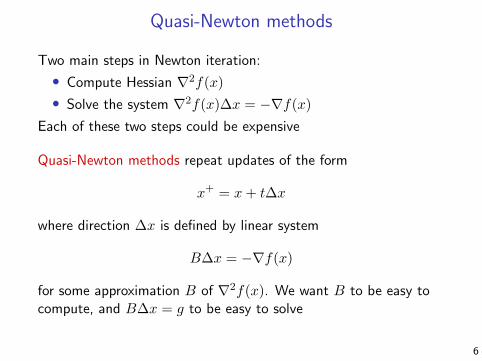
Quasi-Newton methods
Two main steps in Newton iteration:
• Compute Hessian ∇2f(x)
• Solve the system ∇2f(x)∆x = −∇f(x)
Each of these two steps could be expensive
Quasi-Newton methods repeat updates of the form
x+ = x+ t∆x
where direction ∆x is defined by linear system
B∆x = −∇f(x)
for some approximation B of ∇2f(x). We want B to be easy tocompute, and B∆x = g to be easy to solve
6

Some history
• In the mid 1950s, W. Davidon was a mathematician/physicistat Argonne National Lab
• He was using coordinate descent on an optimization problemand his computer kept crashing before finishing
• He figured out a way to accelerate the computation, leadingto the first quasi-Newton method (soon Fletcher and Powellfollowed up on his work)
• Although Davidon’s contribution was a major breakthrough inoptimization, his original paper was rejected
• In 1991, after more than 30 years, his paper was published inthe first issue of the SIAM Journal on Optimization
• In addition to his remarkable work in optimization, Davidonwas a peace activist (see the book “The Burglary”)
7

Quasi-Newton template
Let x(0) ∈ Rn, B(0) � 0. For k = 1, 2, 3, . . ., repeat:
1. Solve B(k−1)∆x(k−1) = −∇f(x(k−1))
2. Update x(k) = x(k−1) + tk∆x(k−1)
3. Compute B(k) from B(k−1)
Different quasi-Newton methods implement Step 3 differently. Aswe will see, commonly we can compute (B(k))−1 from (B(k−1))−1
Basic idea: as B(k−1) already contains info about the Hessian, usesuitable matrix update to form B(k)
Reasonable requirement for B(k):
∇f(x(k)) = ∇f(x(k−1)) +B(k)(x(k) − x(k−1))
8

Secant equation
We can equivalently write latter condition as
∇f(x+) = ∇f(x) +B+(x+ − x)
Letting y = ∇f(x+)−∇f(x), and s = x+ − x this becomes
B+s = y
This is called the secant equation
In addition to the secant equation, we want:
• B+ to be symmetric
• B+ to be “close” to B
• B � 0⇒ B+ � 0
9

Symmetric rank-one update
Let’s try an update of the form
B+ = B + auuT
The secant equation B+s = y yields
(auT s)u = y −Bs
This only holds if u is a multiple of y −Bs. Putting u = y −Bs,we solve the above, a = 1/(y −Bs)T s, which leads to
B+ = B +(y −Bs)(y −Bs)T
(y −Bs)T s
called the symmetric rank-one (SR1) update
10

How can we solve B+∆x+ = −∇f(x+), in order to take nextstep? In addition to propagating B to B+, let’s propagateinverses, i.e., C = B−1 to C+ = (B+)−1
Sherman-Morrison formula:
(A+ uvT )−1 = A−1 − A−1uvTA−1
1 + vTA−1u
Thus for the SR1 update the inverse is also easily updated:
C+ = C +(s− Cy)(s− Cy)T
(s− Cy)T y
In general, SR1 is simple and cheap, but has key shortcoming: itdoes not preserve positive definiteness
11

Broyden-Fletcher-Goldfarb-Shanno update
Instead of a rank-one update to B, let’s try a rank-two update
B+ = B + auuT + bvvT
Using secant equation B+s = y gives
y −Bs = (auT s)u+ (bvT s)v
Setting u = y, v = Bs and solving for a, b we get
B+ = B − BssTB
sTBs+yyT
yT s
called the Broyden-Fletcher-Goldfarb-Shanno (BFGS) update
12

Woodbury formula (generalization of Sherman-Morrison):
(A+ UDV )−1 = A−1 −A−1U(D−1 + V A−1U)−1V A−1
Applied to our case, with
U = V T =[Bs y
], D =
[−1/(sTBs) 0
0 1/(yT s)
]
then after some algebra we get a rank-two update on C:
C+ =
(I − syT
yT s
)C
(I − ysT
yT s
)+ssT
yT s
The BFGS update is thus still quite cheap, O(n2) per update
13

Positive definiteness of BFGS update
Importantly, unlike SR1, the BFGS update preserves positivedefiniteness under appropriate conditions
Assume yT s = (∇f(x+)−∇f(x))T (x+ − x) > 0 (recall that e.g.strict convexity will imply this condition) and C � 0
Then consider the term
xTC+x =
(x− sTx
yT sy
)TC
(x− sTx
yT sy
)+
(sTx)2
yT s
Both terms are nonnegative; second term is only zero whensTx = 0, and in that case first term is only zero when x = 0
14
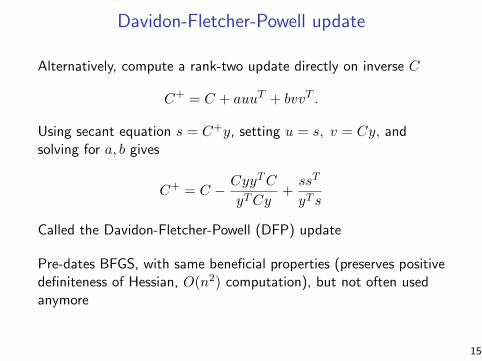
Davidon-Fletcher-Powell update
Alternatively, compute a rank-two update directly on inverse C
C+ = C + auuT + bvvT .
Using secant equation s = C+y, setting u = s, v = Cy, andsolving for a, b gives
C+ = C − CyyTC
yTCy+ssT
yT s
Called the Davidon-Fletcher-Powell (DFP) update
Pre-dates BFGS, with same beneficial properties (preserves positivedefiniteness of Hessian, O(n2) computation), but not often usedanymore
15

Broyden class
SR1, BFGS, and DFP are some of numerous possiblequasi-Newton updates. The Broyden class of updates is defined by:
B+ = (1− φ)B+BFGS + φB+
DFP, φ ∈ R
By putting v = y/(yT s)−Bs/(sTBs), we can rewrite the above as
B+ = B − BssTB
sTBs+yyT
yT s+ φ(sTBs)vvT
Note:
• BFGS corresponds to φ = 0
• DFS corresponds to φ = 1
• SR1 corresponds to φ = yT s/(yT s− sTBs)
16

Convergence analysis
Assume that f convex, twice differentiable, having dom(f) = Rn,and additionally
• ∇f is Lipschitz with parameter L
• f is strongly convex with parameter m
• ∇2f is Lipschitz with parameter M
(same conditions as in the analysis of Newton’s method)
Theorem: Both BFGS and DFP, with backtracking line search,converge globally. Furthermore, for all k ≥ k0,
‖x(k) − x?‖2 ≤ ck‖x(k−1) − x?‖2
where ck → 0 as k →∞. Here k0, ck depend on L,m,M
This is called local superlinear convergence
17

Example: Newton versus BFGS
Example from Vandenberghe’s lecture notes: Newton versus BFGSon LP barrier problem, for n = 100, m = 500
minx
cTx−m∑
i=1
log(bi − aTi x)
Example
minimize cTx �mX
i=1
log(bi � aTi x)
n = 100, m = 500
0 2 4 6 8 10 1210�12
10�9
10�6
10�3
100
103
k
f(x
k)�
f?
Newton
0 50 100 15010�12
10�9
10�6
10�3
100
103
k
f(x
k)�
f?
BFGS
• cost per Newton iteration: O(n3) plus computing r2f(x)
• cost per BFGS iteration: O(n2)
Quasi-Newton methods 2-10
Recall Newton update is O(n3), quasi-Newton update is O(n2).But quasi-Newton converges in less than 100 times the iterations
18
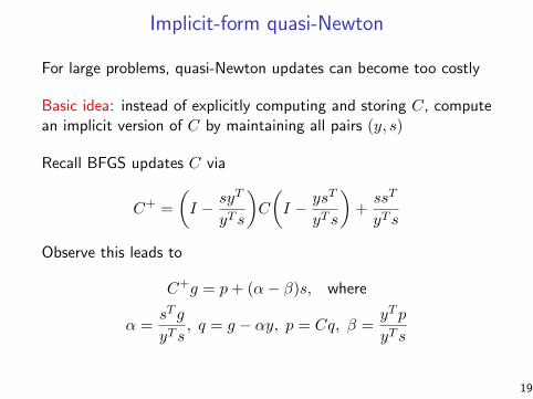
Implicit-form quasi-Newton
For large problems, quasi-Newton updates can become too costly
Basic idea: instead of explicitly computing and storing C, computean implicit version of C by maintaining all pairs (y, s)
Recall BFGS updates C via
C+ =
(I − syT
yT s
)C
(I − ysT
yT s
)+ssT
yT s
Observe this leads to
C+g = p+ (α− β)s, where
α =sT g
yT s, q = g − αy, p = Cq, β =
yT p
yT s
19
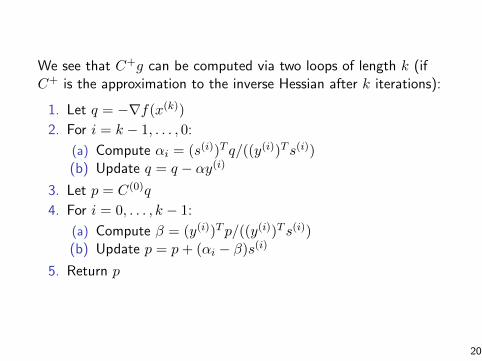
We see that C+g can be computed via two loops of length k (ifC+ is the approximation to the inverse Hessian after k iterations):
1. Let q = −∇f(x(k))
2. For i = k − 1, . . . , 0:
(a) Compute αi = (s(i))T q/((y(i))T s(i))(b) Update q = q − αy(i)
3. Let p = C(0)q
4. For i = 0, . . . , k − 1:
(a) Compute β = (y(i))T p/((y(i))T s(i))(b) Update p = p+ (αi − β)s(i)
5. Return p
20

Limited memory BFGS
Limited memory BFGS (LBFGS) simply limits each of these loopsto be length m:
1. Let q = −∇f(x(k))
2. For i = k − 1, . . . , k −m:
(a) Compute αi = (s(i))T q/((y(i))T s(i))(b) Update q = q − αy(i)
3. Let p = C(k−m)q
4. For i = k −m, . . . , k − 1:
(a) Compute β = (y(i))T p/((y(i))T s(i))(b) Update p = p+ (αi − β)s(i)
5. Return p
In Step 3, C(k−m) is our guess at C(k−m) (which is not stored). Apopular choice is C(k−m) = I, more sophisticated choices exist
21

Stochastic quasi-Newton methods
Consider now the problem
minx
Eξ[f(x, ξ)]
for a noise variable ξ. Tempting to extend previous ideas and takestochastic quasi-Newton updates of the form:
x(k) = x(k−1) − tkC(k−1)∇f(x(k−1), ξk)
But there are challenges:
• Can have at best sublinear convergence (recall lower bound byNemirovski et al.) So is additional overhead of quasi-Newton,worth it, over plain SGD?
• Updates to C depend on consecutive gradient estimates; noisein the gradient estimates could be a hindrance
22
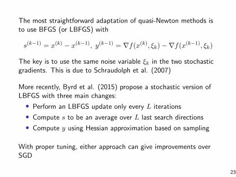
The most straightforward adaptation of quasi-Newton methods isto use BFGS (or LBFGS) with
s(k−1) = x(k) − x(k−1), y(k−1) = ∇f(x(k), ξk)−∇f(x(k−1), ξk)
The key is to use the same noise variable ξk in the two stochasticgradients. This is due to Schraudolph et al. (2007)
More recently, Byrd et al. (2015) propose a stochastic version ofLBFGS with three main changes:
• Perform an LBFGS update only every L iterations
• Compute s to be an average over L last search directions
• Compute y using Hessian approximation based on sampling
With proper tuning, either approach can give improvements overSGD
23

Example from Byrd et al. (2015):
the particular implementation [13] of one of the coordinate descent (CD) methods ofTseng and Yun [26].
Figure 1 reports the performance of SGD (with � = 7) and SQN (with � = 2),as measured by accessed data points. Both methods use a gradient batch size ofb = 50; for SQN we display results for two values of the Hessian batch size bH , andset M = 10 and L = 10. The vertical axis, labeled fx, measures the value of theobjective (4.1); the dotted black line marks the best function value obtained by thecoordinate descent (CD) method mentioned above. We observe that the SQN methodwith bH = 300 and 600 outperforms SGD, and obtains the same or better objectivevalue than the coordinate descent method.
0 0.5 1 1.5 2 2.5 3
x 105
10!2
10!1
100
fx versus accessed data points
adp
fx
SGD: b = 50, ! = 7
SQN: b = 50, ! = 2, bH = 300
SQN: b = 50, ! = 2, bH = 600
CD approx min
SQN vs SGD on Synthetic Binary Logistic Regressionwith n = 50 and N = 7000
Figure 1: Illustration of SQN and SGD on the synthetic dataset. The dotted blackline marks the best function value obtained by the coordinate descent (CD) method.For SQN we set M = 10, L = 10 and bH = 300 or 600.
16
24

References and further reading
• L. Bottou, F. Curtis, J. Nocedal (2016), “Optimizationmethods for large-scale machine learning”
• R. Byrd, S. Hansen, J. Nocedal, Y. Singer (2015), “Astochastic quasi-Newton method for large-scale optimization”
• J. Dennis and R. Schnabel (1996), “Numerical methods forunconstrained optimization and nonlinear equations”
• J. Nocedal and S. Wright (2006), “Numerical optimization”,Chapters 6 and 7
• N. Schraudolph, J. Yu, S. Gunter (2007), “A stochasticquasi-Newton method for online convex optimization”
• L. Vandenberghe, Lecture notes for EE 236C, UCLA, Spring2011-2012
25


