Quasigeostrophic Turbulence with Explicit Surface Dynamics

Quasigeostrophic Turbulence with Explicit Surface Dynamics: Application to theAtmospheric Energy Spectrum

ROSS TULLOCH AND K. SHAFER SMITH

Center for Atmosphere Ocean Science, Courant Institute of Mathematical Sciences, New York University, New York, New York

(Manuscript received 16 October 2007, in final form 6 August 2008)

ABSTRACT

The horizontal wavenumber spectra of wind and temperature near the tropopause have a steep 23 slope at

synoptic scales and a shallower 25/3 slope at mesoscales, with a transition between the two regimes at a

wavelength of about 450 km. Here it is demonstrated that a quasigeostrophic model driven by baroclinic

instability exhibits such a transition near its upper boundary (analogous to the tropopause) when surface

temperature advection at that boundary is properly resolved and forced. To accurately represent surface

advection at the upper and lower boundaries, the vertical structure of the model streamfunction is decom-

posed into four parts, representing the interior flow with the first two neutral modes, and each surface with its

Green’s function solution, resulting in a system with four prognostic equations. Mean temperature gradients

are applied at each surface, and a mean potential vorticity gradient consisting both of b and vertical shear is

applied in the interior. The system exhibits three fundamental types of baroclinic instability: interactions

between the upper and lower surfaces (Eady type), interactions between one surface and the interior

(Charney type), and interactions between the barotropic and baroclinic interior modes (Phillips type). The

turbulent steady states that result from each of these instabilities are distinct, and those of the former two

types yield shallow kinetic energy spectra at small scales along those boundaries where mean temperature

gradients are present. When both mean interior and surface gradients are present, the surface spectrum

reflects a superposition of the interior-dominated 23 slope cascade at large scales, and the surface-dominated

25/3 slope cascade at small scales. The transition wavenumber depends linearly on the ratio of the interior

potential vorticity gradient to the surface temperature gradient, and scales with the inverse of the defor-

mation scale when b 5 0.

1. Introduction

The horizontal kinetic energy and potential temper-

ature variance spectra near the tropopause, observed

during the Global Atmospheric Sampling Program

(GASP) and documented in Nastrom and Gage (1985,

hereafter NG85), exhibit a shallow plateau at the largest

wavelengths (10 000–3000 km), a steep 23 spectral

slope on synoptic scales (’ 3000–1000 km), followed by

a smooth transition (at a wavelength of about 450 km)

to a shallow 25/3 spectral slope on the mesoscales

(’ 200–10 km). The large and synoptic scale parts of

the spectra are consistent with stirring by baroclinic

instability near the Rossby deformation wavelength,

feeding a forward cascade of enstrophy with a 23 slope,

as predicted by Charney’s theory of geostrophic turbu-

lence (Charney 1971). The mesoscale shallowing, how-

ever, does not fit easily into this picture; the robustness

of the synoptic-scale slope and its consistency with

geostrophic turbulence theory make the mesoscale

spectral slope difficult to explain.

The key figure from NG85, reproduced in Fig. 1, plots

power density spectra of the zonal wind (u2), meridional

wind (y2), and the potential temperature (u2) as func-

tions of horizontal wavenumber (meridional wind and

potential temperature are offset by one and two orders

of magnitude, respectively). Below wavelengths of

about 5000 km, the zonal and meridional wind spectra

are nearly identical, implying isotropic kinetic energy

[KE; equal to (u2 1 y2)/2] in the synoptic scales and

below. The potential temperature spectrum exhibits the

same spectral slopes and spectral break, but is about

half the magnitude of the spectra of the winds. The

available potential energy (APE), equal to g2/(2Nu0)2u2,

where g is gravity, N is the buoyancy frequency, and

Corresponding author address: K. Shafer Smith, Courant Insti-

tute of Mathematical Sciences, New York University, 251 Mercer

St., New York, NY 10012.

E-mail: [email protected]

450 J O U R N A L O F T H E A T M O S P H E R I C S C I E N C E S VOLUME 66

DOI: 10.1175/2008JAS2653.1

� 2009 American Meteorological Society

u0 is a reference potential temperature, is therefore very

nearly in equipartition with the kinetic energy.1 In the

23 range, equipartition between KE and APE at each

scale is also consistent with the predictions of geo-

strophic turbulence.2 High-resolution general circula-

tion and weather forecasting models yield similar

results, with equipartition in the 23 range, and a shal-

lowing to 25/3 in the mesoscales (Koshyk and Hamilton

2001; Skamarock 2004; Takahashi et al. 2006; Hamilton

et al. 2008).

Numerous theories for the mesoscale spectrum have

been suggested over the past two decades (Lilly 1989;

Vallis et al. 1997; Dewan 1979; VanZandt 1982; Koshyk

et al. 1999; Tung and Orlando 2003a; Lindborg 2005;

Kitamura and Matsuda 2006). Tung and Orlando

(2003a) summarize all these theories, and put forward

their own. In a recent paper, Tulloch and Smith (2006)

also revisit the proposed mechanisms for the mesoscale

shallowing, and propose a new one, based on a ‘‘toy’’

model that captures many aspects of the observations.

The model is motivated by the following observations:

(i) the near universality of the spectrum in the midlati-

tude atmosphere implies that synoptic-scale baroclinic

instability is likely the forcing of both the 23 and 25/3

ranges of the spectrum (Tung and Orlando 2003a) and

(ii) the 25/3 part of the spectrum is due to a forward

FIG. 1. Variance power spectra of wind and potential temperature near the tropopause from

GASP aircraft data. The spectra for meridional wind and temperature are shifted one and two

decades to the right, respectively; lines with slopes 23 and 25/3 are entered at the same relative

coordinates for each variable for comparison. Reproduced with permission from Nastrom and

Gage (1985).

1 Using typical upper-tropospheric values u0 5 300 K, N 5 1022

s21, and g 5 9.8 m s22, APE ;2u2, and so the dimensional pre-

factor just accounts for the drop in magnitude of the potential

temperature relative to the winds.2 In quasigeostrophic theory, KE/APE ; (Nhe/f‘e)

2, where ‘e

and he are the (variable) horizontal and vertical scales, respec-

tively, of the eddying motion. Charney argued that, neglecting the

influence of boundaries or inhomogeneities in the stratification,

the forward cascade of potential enstrophy should be isotropic in

the space (x, y, Nz/f ). Thus, in the forward cascade, each scale of

eddy motion will maintain a constant aspect ratio ‘e/he ; N/f, in-

dependent of scale, so KE/APE ;1.

FEBRUARY 2009 T U L L O C H A N D S M I T H 451

energy cascade (Cho and Lindborg 2001; Tung and

Orlando 2003b). The physical idea proposed is that

advection of temperature perturbations at the tropo-

pause leads to a forward cascade of temperature vari-

ance, resulting in 25/3 kinetic and potential energy

spectra at mesoscales, as predicted by surface quasi-

geostrophic theory (SQG; Blumen 1978; Held et al.

1995). This is rationalized by the analysis of Juckes

(1994), who showed that tropopause temperature

anomalies account for about 80% of the tropospheric

eddy field. The novel aspect of Tulloch and Smith (2006)

was the demonstration that by limiting surface quasi-

geostrophic flow to a finite depth, a natural transition

scale emerges, and when the flow is forced at large scale,

the kinetic energy spectrum slope is 23 between the

forcing and transition scales, and 25/3 below the tran-

sition scale. The transition scale (;NH/f, where N is the

buoyancy frequency, f is the Coriolis parameter, and H

is the depth of the fluid—i.e., the shallow-water defor-

mation scale) is the scale above which the surface sig-

nals can ‘‘feel’’ the lower boundary. The large-scale

limit is that of barotropic flow, and so follows the predic-

tions of two-dimensional turbulence, while the small-scale

limit, where the vertical extent of temperature signals is

much less than H, is that of surface quasigeostrophic flow.

The finite-depth SQG model is compelling because it

leads to a forward cascade of vortical energy, consistent

with observations (Cho and Lindborg 2001; Cho et al.

1999), and the cascade can be generated by large-scale

forcing such as baroclinic instability, ubiquitous through-

out the midlatitudes, thereby accounting for the uni-

versality of the spectra (Nastrom and Gage 1985). Taken

as complete, however, the model has the following de-

ficiencies: (i) it fails to explain the available potential

energy spectrum at synoptic scales (finite-depth surface

quasigeostrophic flow has no significant potential en-

ergy at large scales); (ii) it predicts a transition scale that

is larger than that observed; and (iii) it predicts an ev-

anescent spectrum at small scales when moving down

into the troposphere (midlevel spectral observations in

the troposphere are rare, but there is no evidence for

evanescent decay of energy). These deficiencies, it is

shown here, are removed when interior potential vor-

ticity anomalies are included in the flow.

The surface quasigeostrophic model is derived by

assuming quasigeostrophic scaling, and considering a

special case in which temperature on a horizontal sur-

face is advected and bounded above and/or below by

regions of zero or constant potential vorticity (PV). It is

thus typically assumed that regions of constant PV are

necessary in order to obtain dynamics like those pre-

dicted by surface quasigeostrophic flow. In a companion

paper to this one (Tulloch and Smith 2009), we show

that this restriction is not necessary, and that surface

effects of the type predicted by SQG occur whenever

temperature perturbations are forced and sufficiently

resolved in the vertical (see also McWilliams and Chow

1981; Fox-Rabinovitz and Lindzen 1993; Solomon and

Lindzen 2000; Snyder et al. 2003).

In the present paper, we show that surface effects can

be retained without high-vertical resolution, so long as

representations of the surface dynamics are included

explicitly in the model. The method proposed follows

recent work by Lapeyre and Klein (2006), but goes back

to Hoskins et al. (1985) and perhaps earlier papers (see

also, e.g., Holopainen and Kaurola 1991; Davies and

Bishop 1994). The method is based on the decomposi-

tion of the streamfunction into components that solve

the interior PV and two boundary temperature prob-

lems, separately; it is an equivalent alternative to

Bretherton’s (1966) use of delta function layers of PV at

rigid surfaces (and both methods can be understood in

terms of a Green’s function, as shown in appendix A).

The decomposition method, however, has the advan-

tages that it allows for the construction of a fully non-

linear numerical model that both captures the surface

dynamics accurately (without need for high vertical

resolution), and makes explicit their interaction with the

interior flow. The Bretherton approach, by contrast,

relies on finite-difference representations of the delta

sheets of PV, with the accompanying pitfalls described

in the previous paragraph.

We specialize within this model framework to include

just enough complexity to address the observed atmo-

spheric energy spectra, at the transition to subsynoptic

scales. The simplified model advects the barotropic and

baroclinic interior flow, and the upper and lower surface

temperatures. In spectral space, the vertical structures

for the four variables are separable from their time-

dependent parts. Assuming constant stratification N2,

these modes can be easily computed analytically. The

resulting model is very similar to one developed by

G. Flierl (2007, personal communication), with some

differences, but to our knowledge these are the only

examples of fully nonlinear, forward model imple-

mentations using the decomposition approach. This

two-mode, two-surface model (hereafter referred to as

the TMTS model) is effectively a hybrid of the Phillips

and Eady models, and so can represent baroclinic in-

stability generated from barotropic–baroclinic interac-

tions (as in the standard two-layer Phillips model),

surface–surface interactions (as in the Eady model),

and from interactions between either surface and the

interior (as in the Charney model of baroclinic insta-

bility). It is hoped that, besides its application in this

paper, the analytical tractability of this four-variable


model may allow for its use as a pedagogical tool (we

thank an anonymous reviewer for suggesting this).

The TMTS model is designed to understand the ob-

served atmospheric energy spectrum at subsynoptic

scales; a corollary is that high vertical resolution is not

needed to understand the transition to a shallow spec-

trum, so long as surface dynamics are explicitly repre-

sented. On the other hand, the model may be deficient

for applications that require a more realistic represen-

tation of the vertical structure of eddy fluxes at the

synoptic and planetary scale.

Both linear instabilities and nonlinear turbulent

steady states of the TMTS model are explored. Nu-

merical simulations of turbulent steady states reveal

spectra similar to the observed atmospheric spectra in

Fig. 1, and can be understood as resulting from the su-

perposition of a 23 slope, due to interior-forced geo-

strophic turbulence at large scales, and a 25/3 slope,

due to surface-forced SQG turbulence at small scales.

This structure is in accordance with Fig. 7 from Lindborg

(1999) which shows that the NG85 spectrum is well fit by

a superposition. Rather than resulting from surface

signals feeling the bottom boundary, the transition here

occurs where the surface cascade starts to dominate the

interior cascade. The scale at which the transition oc-

curs, it is shown, is a function of the ratio of interior PV

to surface temperature gradients. The transition scale

predicted by applying the formula to the National

Centers for Environmental Prediction (NCEP) rean-

alysis data is very close to the observed transition scale.

In summary, this paper is presented with the follow-

ing major goals in mind:

1) to show the usefulness of the streamfunction-de-

composition method in constructing numerical

models that accurately represent surface dynamics;

2) to derive a simplified model (TMTS) within this

framework that captures all major types of baroclinic

instability;

3) to use this model to demonstrate that surface dy-

namics at the tropopause may explain the transition

to a shallow energy spectrum at subsynoptic scales;

and

4) to provide a theory for the transition scale observed

in the atmospheric energy spectra.

The paper is organized as follows: In section 2 we

review the quasigeostrophic equations, including ad-

vection by mean wind and the appropriate boundary

conditions, and derive a simplified model consisting of

two interior and two surface modes (i.e., the TMTS

model). Solutions to the associated linear instability

problem are presented in section 3, partly in order to

characterize the parameter space of interest, but also to

demonstrate the ability of the model to represent the

basic types of baroclinic instability. The results of a se-

ries of nonlinear simulations are presented in section 4,

and a theory for the transition scale that is consistent

with both simulated and observed data is proposed.

Successes and shortcomings of the theory are discussed

in section 5, along with plans for future work.

2. A quasigeostrophic model for surface–interiorinteraction

For the sake of providing a self-contained presenta-

tion, the quasigeostrophic equations are stated and the

two-internal, two-surface mode approximation is de-

rived as a stand-alone model. A more complete treat-

ment is discussed briefly in Tulloch and Smith (2009),

and implications for more complex interior structure

(representative of the ocean) will be explored in a fu-

ture paper.

a. The quasigeostrophic equations

The quasigeostrophic equations for a fluid bounded in

the vertical by flat, rigid surfaces at z 5 H and z 5 0, and

assuming a mean baroclinic zonal wind U(z), are

qt 1 Jðc; qÞ1 Uqx 1 yQy 5 0 for 0 , z , H; ð1aÞ

ut 1 Jðc; uÞ1 Uux 1 yQy 5 0 for z 5 H; and ð1bÞ

ut 1 Jðc; uÞ1 Uux 1 yQy 5� r=2c for z 5 0; ð1cÞ

where c (x, y, z, t) is the geostrophic streamfunction,

u 5 (u, y) 5 (2cy, cx) is the horizontal velocity, = 5

(›x, ›y), J(A, B) 5 AxBy 2 AyBx is the two-dimensional

Jacobian operator, and r 5 dEkN2/f is the (linear) Ek-

man drag coefficient, where dEk is proportional to the

thickness of the Ekman layer, N is the buoyancy fre-

quency, and f is the Coriolis parameter. The potential

vorticity q and potential temperature u are related to

the streamfunction by

q 5 =2c 1 Gc and ujz50;H 5 cz jz50;H ; ð2Þ

respectively, where G [ ›z f 2/N2›z is the stretching op-

erator. The temperature variable u is scaled by g/fu0,

where g is gravitational acceleration and u0 is a refer-

ence temperature, and so the advected ‘‘temperatures,’’

as well as the linear drag coefficient r, have the units

of velocity. Note also that in an atmospheric context,

z is a pseudoheight, or modified pressure coordinate

(Hoskins and Bretherton 1972). The mean gradients of

potential vorticity and potential temperature are related

to the mean wind and Coriolis gradient b by


Qy 5 b� GU; Qyð0Þ5 �Uzð0Þ; QyðHÞ5 �UzðHÞ:ð3Þ

Since the potential vorticity inversion problem in (2)

is linear we can decompose the total streamfunction into

three components:

c 5 c I1cT1cB; ð4Þ

where each of the above depends on (x, y, z, t), the

interior (I) part c I solves

=2c I 1 Gc I 5 q; c Izjz5H 5 0; c I

zjz50 5 0; ð5Þ

and the top (T) and bottom (B) surface components cT

and cB solve

=2cT 1 GcT 5 0; cTz jz5H 5 ujz5H ; cT

z jz50 5 0; and

ð6aÞ

=2cB 1 GcB 5 0; cBz jz5H 5 0; cB

z jz50 5 ujz50 :

ð6bÞ

Similar decompositions have been used in the past; for

example, Davies and Bishop (1994) applied such a de-

composition to edge waves with interior PV distributions,

and Lapeyre and Klein (2006) used it as framework

through which to interpret oceanic surface signals. See

appendix A for a comparison between this stream-

function decomposition and the method that considers

the boundary temperature distribution as sheets of po-

tential vorticity (Bretherton 1966; Heifetz et al. 2004).

b. Modal representation

To generate a numerical model that will aid under-

standing of the atmospheric energy spectrum, the fol-

lowing simplifying assumptions are made: (i) horizontal

boundary conditions are taken to be periodic, consistent

with the assumption of horizontal homogeneity in the

synoptic scales and below; (ii) the vertical structure of

the interior flow can be represented with the gravest two

standard vertical modes (barotropic and baroclinic);

(iii) the stratification N2 is constant in the troposphere

and infinite above, so that the tropopause itself is a rigid

lid (this assumption can be relaxed, following Juckes

1994); and (iv) the mean velocity is zonal, horizontally

constant and projects onto the baroclinic and surface

modes (with no barotropic component).

Assumption (i) allows a Fourier representation in the

horizontal, and so the full streamfunction can be written as

cðx; y; z; tÞ5 �K

eiK�x cI

Kðz; tÞ1 cT

Kðz; tÞ1 cB

Kðz; tÞh i

;

ð7Þ

where K 5 (k, ‘) is the horizontal wavenumber and K 5

|K|. Hats denote spectral coefficients, and from hereaf-

ter, where no confusion can arise the subscript K will be

dropped.

Assumption (ii) allows for the expansion of the inte-

rior part in modes c Iðz; tÞ 5 c btðtÞ1c bcðtÞfðzÞ, where,

where bt means barotropic, bc means baroclinic, and

f(z) is the first baroclinic mode, that is, the gravest,

nonconstant eigenfunction solution to

Gf 5 �l2f fordf

dzð0;HÞ5 0: ð8Þ

It is straightforward, but cumbersome, to use more

vertical modes in the interior. With assumption (iii), the

mode is

fðzÞ5ffiffiffi2p

cospz

H

� �and l 5

pf

NH: ð9Þ

Note for future reference that hfi 5 h(f)3i 5 0 and

h(f)2i 5 1, where h�i 5 H�1ÐH

0 � dz is shorthand for a

vertical average.

In the spectral domain, the surface inversion prob-

lems in (6a) and (6b) are separable, and so

cTðz; tÞ 5 c tðtÞf tðzÞ and c Bðz; tÞ 5 c bðtÞfbðzÞ, where

lowercase t (top) and b (bottom) are used to distinguish

the separated variables and ft,b (which we call the

‘‘surface modes’’) satisfy

ð�K21GÞft 5 0;dft

dzð0Þ5 0;

dft

dzðHÞ5 ut

ct;

ð�K21GÞfb 5 0;dfb

dzð0Þ5 ub

cb;

dfb

dzðHÞ5 0: ð10Þ

Unlike the interior modes, the surface modes will de-

pend on the magnitude of the wavevector, K. Note also

that ft(H) 5 1 and fb(0) 5 1, so that cTðH; tÞ 5 c tðtÞand cBð0; tÞ 5 cbðtÞ: Since N2 is constant, the solutions

are easily computed; they are

ftðzÞ5 cosh mz

H

� �sechm; ð11aÞ

fbðzÞ5 cosh mz�H

H

� �sechm; ð11bÞ

where m 5 KNH/f.

c. Inversion relations

Given the surface modes, the top and bottom tem-

perature fields are obtained by setting z 5 H in ft and

z 5 0 in fb, leading to

utðtÞ[ ujz5H 5�m

Htanh m

�ctðtÞ and ð12aÞ


ubðtÞ[ujz50 5�� m

Htanh m

�cbðtÞ: ð12bÞ

Expanding the potential vorticity in interior modes

qðx; y; z; tÞ 5 qbtðtÞ1qbcðtÞfðzÞ yields

qbtðtÞ5 �K2cbtðtÞ; ð13aÞ

qbcðtÞ5 �K2 m21p2

m2cbcðtÞ: ð13bÞ

Given the potential vorticity and surface temperature

fields, (12) and (13) can be inverted to give the four

streamfunction components, and the full stream-

function is thus

cðx; y; z; tÞ5 �K

eiK�x�cbtK ðtÞ1 cbc

K ðtÞfðzÞ

1 c tKðtÞft

KðzÞ1 c bKðtÞfb

KðzÞ�: ð14Þ

The prognostic equations for the barotropic and bar-

oclinic potential vorticity components in (13) are de-

rived by expanding the streamfunction and potential

vorticity in (1a) using (14), then projecting onto the

barotropic mode by integrating in the vertical, and onto

the baroclinic mode by integrating f times the expres-

sion. Each surface temperature equation is obtained by

evaluating the full advecting streamfunction in (14) at

the vertical level of the surface of interest.

d. Mean field projections

The last step is to project the mean velocity onto the

truncated vertical representation. The mean zonal ve-

locity must in general satisfy (3) (but we set V 5 0), and

to be consistent with the dynamic variables q and u we

decompose the mean zonal velocity into interior and

surface components U(z) 5 UI(z) 1 US(z). The rela-

tionships among the mean fields, however, are some-

what different than that between the eddy fields, due to

the fact U is independent of x and y (i.e., mean relative

vorticity is neglected, consistent with the assumption of

local homogeneity). Assumption (iv) gives us that UI 5

Ubcf(z), where f(z) is given by (9). Derivatives of UI

evaluated at 0 and H vanish and therefore US must

satisfy the boundary conditions, given arbitrary Qty and

Qby . We thus demand that the surface component solves

GUS 5 A;dUS

dzðHÞ5 �Qt

y; anddUS

dzð0Þ5 �Qb

y :

ð15Þ

In analogy with the decomposition of the eddy com-

ponents in (4) and (6), one might expect to demand that

GUS 5 0. However, this can only be satisfied if Qty 5 Qb

y

(therefore it would also be impossible to separate US

into Ut 1 Ub). Instead, here we demand that the right-

hand side, A, be a constant, and that the vertical mean

of the surface velocity vanish, hUSi 5 0. The result is

that

A 5f 2

HN2

!DQy; DQy [ Qt

y �Qby ;

which vanishes only when upper and lower temperature

gradients are equal, and

USðzÞ5�Qby z�H

2

� �1DQy

z2

2H�H

6

� �: ð16Þ

The full mean velocity is therefore U(z) 5 Ubcf(z) 1

US(z). [A Green’s function approach to the mean ve-

locity problem is illustrated in appendix A.]

That A 6¼ 0 means that the surface velocity field US

induces an interior mean PV gradient; the total mean

potential vorticity gradient is therefore

Qy 5 b� GU 5 b 1 L�2D ½HDQy 1

ffiffiffi2p

p2Ubc cospz

H

� ��;

ð17Þ

where LD 5 NH/f is the deformation scale and (9) was

used [note that the first baroclinic deformation wave-

number, defined in (9), is l 5 p/LD].

e. The two-mode, two-surface model

Putting all the prior results together, the full set of

spectral prognostic equations can now be written as

utt 1 Jðcjz5H ; u

tÞ1 ik½UðHÞut 1 Qtycjz5H �5 0; ð18aÞ

ubt 1 Jðcjz50; u

bÞ1 ik½Uð0Þub 1 Qby cjz50�5 rK2cjz50;

ð18bÞ

qbtt 1J c

; qbt

� �1J fc

; qbc

� �and

1ik½hfUiqbc1�b� GUSÞhci1l2Ubchfci�5 0; ð18cÞ

qbct 1J

�fc

; qbt�

1J ffc

; qbc� �

1ik½ fUh iqbt1 ffUh iqbc1 b� GUS� �

fc

1l2Ubc ffc

�5 0

;

ð18dÞ

where J is shorthand for the sum over wavenumbers of

the Jacobian terms, and the streamfunction evaluated at

the upper and lower surfaces, respectively, is


cjz5H 5 cbt �ffiffiffi2p

cbc1ct1cb sech m

cjz50 5 cbt1ffiffiffi2p

cbc1ct sech m1cb:

The vertical integrals and projections of the total

streamfunction and mean shear onto the baroclinic

mode (e.g., fc

) are derived and stated in appendix B.

Equations (18) sacrifice the ability to represent high

vertical modes of the interior flow, but retain an accu-

rate description of surface motions, even when such

motions have very small vertical penetration into the

interior. The projection onto a truncated set of interior

modes, plus surface modes, allows for a compact model

that can be numerically integrated with much greater

efficiency than a high-vertical resolution gridded model.

The goal in developing this model is twofold: (i) to

derive a simple model that retains all basic types of

baroclinic instability, and (ii) to demonstrate that aug-

mentation of the two-layer model with surface modes is

sufficient to explain the spectrum of energy in the at-

mospheric mesoscales. The model is not sufficient to

explore more complex vertical structures, and this will

be taken up in a future paper.

3. Linear instability calculation

Assuming horizontally constant, baroclinic zonal

mean flow, the quasigeostrophic equations in (1) are

linearly unstable to small perturbations under at least

one of the following conditions (Charney and Stern

1962; Pedlosky 1964): (i) Qy 5 0, and Qty and Qb

y are

both nonzero and have the same sign (as in the model of

Eady 1949); (ii) Qy changes sign in the interior and the

boundary gradients are zero (as in the model of Phillips

1954); or (iii) Qy 6¼ 0 and either the upper surface gra-

dient has the same sign, or the lower surface gradient

has the opposite sign as Qy (as in the model of Charney

1947). The standard two-layer model of Phillips admits

only instabilities of the second type, yet has arguably

been more widely used than either the Charney or Eady

model, due to its analytical tractability, wide parameter

range possibilities, inclusion of b, and the ease with

which it can be numerically simulated. The TMTS

model in (18) derived in section 2 is intended to retain

those positive features of the two-layer model while

additionally admitting the two missing instability types

[(i) and (iii)]. Here we have the following goals: to

demonstrate that all of types (i)–(iii) are captured in the

two-mode, two-surface model presented in section 2

(and this requires redoing some standard calculations);

and to compute the linear instability of the flow that will

be used to drive the nonlinear turbulence simulations

presented in section 4.

To compute the baroclinic instability of the TMTS

model, the nonlinear terms are neglected and a normal-

mode wave solution is assumed: ðc t; c b; cbt; c bcÞ 5

<u exp(2ivt), where u 5 ðut; ub; ubt; ubcÞ and the meridi-

onal wavenumber ‘ is set to 0. Specifically, we solve the

eigenvalue problem cu 5 Au where A is a 4 3 4 matrix

(given in appendix C) and c 5 v/k. The growth rate vi 5

kci of unstable modes depends on b, the magnitude of

the internal velocity shear U bc, and on the boundary

temperature gradients Qt;by . We nondimensionalize the

parameter space of the problem with horizontal length

scale LD, vertical length scale H, and a velocity scale U0.

Horizontal wavenumbers K are already expressed

nondimensionally as m 5 KLd almost everywhere they

appear. The nondimensional Coriolis gradient is ~b [

bL2d=U0 and the velocity parameters of the problem are

U bc/U0 and ðH=U0ÞQ t;by 5 �ðH=U0ÞUt;b

z :

Figures 2 and 3 show numerically computed growth

rates and amplitudes of eigenfunctions of the linearized

TMTS model as functions of m and ~b. Figure 2a shows

the growth rates given equal, nonzero boundary tem-

perature gradients ðH=U0ÞQ ty 5 ðH=U0ÞQ b

y 5�1; and

zero interior shear, U bc 5 0. The Eady problem corre-

sponds to the line ~b 5 0, and along this line, max(vi)Ld/

U0 ’ 0.31, as expected. For ~b6¼ 0 boundary gradients

interact with Qy 5 b in the interior, which results in

Charney-type instabilities at small scales and a trun-

cated Green (1960) mode at large scales (see also

Lindzen 1994, who considered the effects of altering the

mean state to retain 0 interior PV with b). Figure 2b

shows the amplitudes, as functions of height, that cor-

respond to the fastest-growing modes at various loca-

tions in the ðm; ~bÞ plane, as indicated by symbols in Fig.

2a. The plus symbol, for example, corresponds to the

location of maximum growth in the Eady problem

ð~b 5 0Þ, and has the expected symmetric amplitude,

peaked at the boundaries [cosh mz/H 2 (U0/mc) sinh

mz/H]. The triangle is located in the Green-mode re-

gion, and has a vertical structure that is comparable to

Fig. 6 of Green (1960). The circle is in the bottom

Charney-mode region and its vertical structure is, like-

wise, comparable to that expected for the Charney

problem (see, e.g., Pedlosky 1987, his Fig. 7.8.5).

Figure 2c shows the growth rates for the pure interior

shear problem, with Qty 5 Qb

y 5 0 and Ubc=U0 5

�1ffiffiffi2p

p� �

and Fig. 2d shows its vertical structure. This is

the standard two-mode Phillips problem with max

ðviÞLd= Ubc 5

ffiffiffi2p� 1

� �p; and so the chosen value of

Ubc/U0 gives max ðviÞLd=U0 5 1� 1ffiffiffi2p

5 0:29, which

is close to the maximum growth rate for the Eady

problem. As expected, there is no longwave cutoff for~b 5 0. For large enough ~b, instability is suppressed, and

the amplitude is peaked at the boundaries, but is large


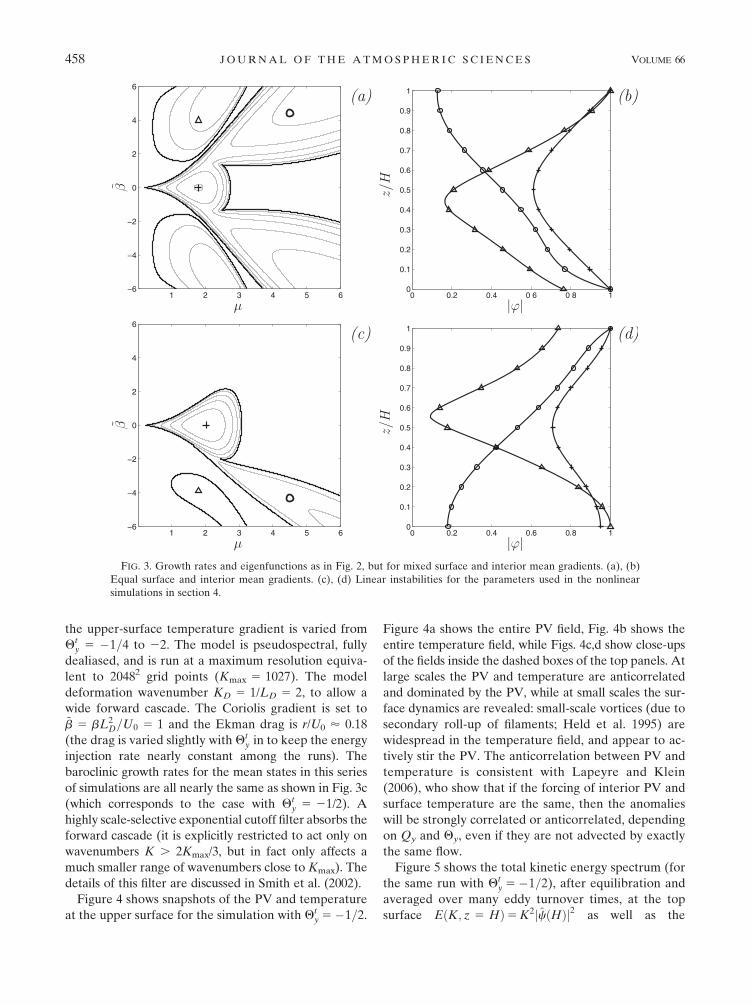
throughout the depth of the fluid. Figure 3a shows the

growth rate for equally weighted surface and interior

forcing ðH=U0ÞQty 5 ðH=U0ÞQb

y 5 �1 and Ubc=U0 5

�1=ffiffiffi2p

p� �

; comparison to Fig. 2a shows that the effect

of the interior shear in this case is primarily to suppress

growth at small scales, for small values of ~b. The vertical

structure of the amplitudes for the three apparent peaks

are similar to those in Figs. 2a,b, except that the am-

plitude corresponding to the ~b 5 0 instability is larger.

Figure 3c shows the growth rate for a mean state with an

upper-surface temperature gradient ðH=U0ÞQty 5 �1=2,

a vanishing lower-surface temperature gradient, and

an interior shear Ubc=U0 5 �4=ffiffiffi2p

p� �

; 4 times larger

than the interior shear used in Fig. 3a. This mean state is

used in the central nonlinear simulation discussed in

the next section. Removing the bottom temperature

gradient has suppressed the large-scale Green modes,

and left only type (iii) (Charney) instabilities at small

scales. The asymmetry at small scales occurs because

the upper-surface temperature gradient and the interior

PV gradient must be of the same sign [consider the PV

gradient in Eq. (17)].

4. Nonlinear simulations

Here we report on the results of a series of simula-

tions made with the fully nonlinear TMTS model in

(18), using parameters relevant to the midlatitude at-

mosphere. In all cases, we set the dimensional param-

eters U0 5 H 5 1, and L 5 2p, so that wavenumber

1 fills the domain. In the primary series, the interior

shear and bottom temperature gradient are held con-

stant at Ubc 5 �4=ffiffiffi2p

p� �

and Qby 5 0, respectively, but

FIG. 2. Growth rates vs nondimensional b and zonal wavenumber are plotted for (a) an Eady-like instability (when~b 5 0) with only mean surface gradients and (c) a Phillips-type instability with only mean interior gradients. Contour

values are vary linearly from 0.05 (thick line) to 0.4 at 0.05 intervals. Note that growth rates have been nondimensionalized

by U0 /Ld. (b), (d) The amplitudes as a function of z for the instability points with the same symbols as in (a) and (c),

respectively.


the upper-surface temperature gradient is varied from

Qty 5 �1=4 to 22. The model is pseudospectral, fully

dealiased, and is run at a maximum resolution equiva-

lent to 20482 grid points (Kmax 5 1027). The model

deformation wavenumber KD 5 1/LD 5 2, to allow a

wide forward cascade. The Coriolis gradient is set to~b 5 bL2

D=U0 5 1 and the Ekman drag is r/U0 ’ 0.18

(the drag is varied slightly with Qty in to keep the energy

injection rate nearly constant among the runs). The

baroclinic growth rates for the mean states in this series

of simulations are all nearly the same as shown in Fig. 3c

(which corresponds to the case with Qty 5 21/2). A

highly scale-selective exponential cutoff filter absorbs the

forward cascade (it is explicitly restricted to act only on

wavenumbers K . 2Kmax/3, but in fact only affects a

much smaller range of wavenumbers close to Kmax). The

details of this filter are discussed in Smith et al. (2002).

Figure 4 shows snapshots of the PV and temperature

at the upper surface for the simulation with Qty 5�1=2.

Figure 4a shows the entire PV field, Fig. 4b shows the

entire temperature field, while Figs. 4c,d show close-ups

of the fields inside the dashed boxes of the top panels. At

large scales the PV and temperature are anticorrelated

and dominated by the PV, while at small scales the sur-

face dynamics are revealed: small-scale vortices (due to

secondary roll-up of filaments; Held et al. 1995) are

widespread in the temperature field, and appear to ac-

tively stir the PV. The anticorrelation between PV and

temperature is consistent with Lapeyre and Klein

(2006), who show that if the forcing of interior PV and

surface temperature are the same, then the anomalies

will be strongly correlated or anticorrelated, depending

on Qy and Qy, even if they are not advected by exactly

the same flow.

Figure 5 shows the total kinetic energy spectrum (for

the same run with Qty 5�1=2), after equilibration and

averaged over many eddy turnover times, at the top

surface EðK; z 5 HÞ5 K2jcðHÞj2 as well as the

FIG. 3. Growth rates and eigenfunctions as in Fig. 2, but for mixed surface and interior mean gradients. (a), (b)

Equal surface and interior mean gradients. (c), (d) Linear instabilities for the parameters used in the nonlinear

simulations in section 4.


components that contribute to the total kinetic energy,

plotted against horizontal wavenumber. The dash–dot

line is the barotropic kinetic energy K2jcbtj2, which is

driven primarily by the interior shear Ubc and has a

steep K23 slope as a result of enstrophy cascading to

small scales. The dashed line is the spectrum of APE at

the upper surface, which is equal to the kinetic energy of

the surface streamfunction K2jctj2 and cascades for-

ward with a shallow K25/3 slope [also see Gkioulekas

and Tung (2007a) for a derivation of equipartition be-

tween KE and APE in SQG turbulence and Gkioulekas

and Tung (2007b) for a proof of the cascade direction].

The solid line is the total kinetic energy spectrum at the

upper surface, which is apparently a superposition of the

barotropic and surface-induced spectra (with some in-

fluence from the baroclinic kinetic energy at large

scales), perhaps as expected from the PV and temper-

ature fields in Fig. 4. There is a transition from K23

interior-dominated dynamics to K25/3 surface-domi-

nated dynamics at a wavenumber that depends on the

relative energy levels in the surface and interior modes,

which in turn depend on the relative strengths of the

surface and interior baroclinic forcings. We also note

that, because the interior dynamics in the numerical

model are truncated at the first baroclinic mode, the

interior APE is concentrated at z 5 H/2, and so the

simulated APE lacks a K23 slope at large scales at or

near the upper surface.

FIG. 4. Snapshots of (a) [close-up in (c)] PV and (b) [close-up in (d)] temperature at the top surface for the

Qty 5 �0:5 case. At large scales q(H) and ut are anticorrelated and driven by the PV dynamics. At small scales q(H) is

dominated by the dynamics of vortices present in ut.


a. The transition scale

Figure 6 shows the upper-surface kinetic energy

spectra for each of the series of simulations in which Qty

is varied from 21/4 to 22. It is apparent that the tran-

sition scale between the steep large-scale spectrum and

the shallow small-scale spectrum is controlled by Qty.

The particular dependence of the transition scale on the

parameters of the problem can be understood as fol-

lows. The upper-level energy spectrum in the forward

enstrophy cascade has the form

EðKÞ5 CEh2=3K�3;

where the rate of enstrophy transfer at z 5 H is

h 5 �QyðHÞ yqjz5H [ kqQyðHÞ2:

The overbar denotes a horizontal average, CE is a

Kolmogorov constant, and we have defined a PV dif-

fusivity kq. The cascade of temperature variance at the

upper surface leads to an available potential energy

spectrum of the form

AðKÞ5 CAe2=3K�5=3; ð19Þ

where the relevant energy flux is

e5�f 2Qt

y

N2yutjz5H [ ku

f Qty

N

!2

:

Here we have defined a second diffusivity ku for the

temperature, and a second Kolmogorov constant for the

temperature cascade.

Assuming equal diffusivities kq’ ku and Kolmogorov

constants CE ’ CA, and solving for the wavenumber

where the two cascades are equal, one finds the upper-

level transition wavenumber

Ktrans ’N

f

QyðHÞQt

y

:

It is instructive to rewrite this expression as

Ktrans ’ L�1C 1L�1

D

Uzð0Þ �UzðHÞ �ffiffiffi2p

p2Ubc=H

UzðHÞj j

;ð20Þ

where (3) and (17) were used to replace the PV and

temperature gradients with shears and

LC 5f

N

UzðHÞj jb

is the Charney length (see, e.g., Pedlosky 1987). The

second expression for Ktrans now has a form similar to

that of the transition wavenumber found by Tulloch and

Smith (2006), L�1D 5 f=NH; except that here (pulling

out a factor f/N) there are two vertical scales, added

in reciprocal: the Charney depth (hC 5 fLC/N) and a

FIG. 5. Energy densities as a function of horizontal wavenumber

for the Qty 5 �0:5 simulation. The kinetic energy density at the

top surface (thick solid) exhibits a transition from 23 where bar-

otropic kinetic energy (dash–dot) dominates to 25/3 at k ’ 100 as

the variance of temperature (long dashed) begins to dominate the

forward cascade.

FIG. 6. Kinetic energy spectra at z 5 H with Qty 5 �2;�1;�0:5;

and 20.25, Ubc 5 �4=ðpffiffiffi2pÞ and H 5 1 at 20482 resolution. Thin

lines are k25/3 and k23 for reference. The small-scale spectra are

approximately 11k25/3, 5k25/3, 1.5k25/3, and 0.45k25/3.


second term corresponding to the fluid depth H times

the relative ratio of surface to total shears. In the limit of

no interior or bottom shear, and assuming hC� H, the

vertical scale is just the Charney depth, and Ktrans ’L�1

C : In the limit of b 5 0, the transition scales with the

inverse deformation scale, and if additionally Uz(H)�Ubc/H, then the vertical scale is H ðKtrans ’ L�1

D Þ, as

found in the simpler model of Tulloch and Smith (2006).

The scaling prediction in (20) is tested against the

‘‘measured’’ transition wavenumbers for all simulations

performed (including a third series identical to the

second series, but where the bottom temperature gra-

dient is held fixed at Qby 5 5) in Fig. 7 (see caption for

details of the transition-scale computation). The theory

apparently captures the variation of transition scale

with surface shear quite well. There is a bias toward

underpredicting the measured transition wavenumber

when Ktrans is small, which is perhaps due to halting

scale (or drag) effects in the numerical model, which are

not accounted for in the theory. We also check here that

the results are independent of horizontal resolution.

Figure 8 shows the resulting surface energy spectra for a

series of simulations in which all parameters are held

constant ðQty 5 �0:5Þ, but horizontal resolution is suc-

cessively reduced. The results confirm that the transi-

tion from 23 to 25/3 is independent of numerical

resolution, as well as small-scale filtering.

We can check that the surface energy exhibits an in-

ertial range cascade by computing the energy flux di-

rectly, as a function of the wavenumber. For the series

of simulations in which the upper-surface temperature

gradient is varied, the surface fluxes of available po-

tential energy,

eðKÞ5 f 2

N2

ðK

0

ut Jðc; utÞ dK0; ð21Þ

are shown in Fig. 9. The fluxes are plainly constant, as

suggested.

b. Atmospheric forcing

Using long-term monthly mean data from the NCEP

reanalysis simulations, a mean wind profile is computed

by averaging data from 458N temporally and zonally.

The meridional potential temperature gradients from

the 1000- and 200-mb data (corresponding to H ’ 9.7

km) are computed from zonal and temporal averages at

the same latitude, from which the mean upper- and

lower-level shears are inferred from thermal wind bal-

ance, and the profile US is then computed from the

shears. The interior first baroclinic mean zonal wind is

then approximately the difference between the NCEP

data profile and the surface-induced zonal wind. The

resulting surface shears are Uz(H) 5 5.6 3 1024 s21 and

Uz(0) 5 2.1 3 1023 s21, and the interior baroclinic ve-

locity is Ubc 5 22.6 m s21, corresponding to an interior

shearffiffiffi2p

p2Ubc=H 5 3:7 3 10�3s�1: Using a typical

stratification N 5 1022 s21, one finds LC 5 360 km,

LD 5 950 km, and so Eq. (20) gives Ktrans ’ 1/77 km21

(or the transition wavelength ’ 480 km) as the transi-

tion wavenumber predicted by our scaling theory, which

is quite near the observed atmospheric transition wave-

length of about 450 km.

These mean values are used in a simulation, the re-

sults of which are shown in Fig. 10. Figure 10a shows the

spectra of kinetic energy at the upper surface, the

available potential energy, and the barotropic kinetic

energy. The structure is similar to the spectra in Fig. 5.

The bottom axis is the dimensional wavelength, for

comparison with the Nastrom–Gage spectrum pre-

sented in Fig. 1. The transition wavelength in the sim-

ulation is near 300 km, somewhat smaller than that

predicted above (and smaller than the observed tran-

sition wavelength), but is consistent with the bias of

underpredicting the transition wavenumber when Ktrans

is small, as shown in Fig. 7 and discussed above. Note

FIG. 7. The measured transition wavenumber for all simulations,

defined as where the slope is k27/3, compared with the prediction

from (20). We set L 5 2p, U0 5 H 5 1 for all runs. Asterisks:

Qty 5 Qb

y 5 �5;�3;�1;�0:5; Ubc 5 21, ~b 5 3, KD 5 4; plus

signs: same as asterisks, but Qty 5� 5 for each; circles: Qt

y 5 22,

21, 20.5, 20.25, Qby 5 0;Ubc 5 � 4=ð

ffiffiffi2p

pÞ; ~b 51; KD 5 2; cros-

ses: Qty 5 � 2;�1;�0:5;�0:25; Qb

y 5 0; Ubc 5 20.7, ~b 5 3; and

KD 5 2.


that we have made coarse approximations in choosing

our atmospheric parameters by averaging zonally at a

particular latitude and pressure level, so it is not sur-

prising that there is a discrepancy. The overall energy

level of our simulation is higher than the observed level,

and the temperature variance is less. However, it

should be restated that this is an idealized, doubly pe-

riodic model, designed to represent one aspect of the

turbulent structure of the synoptic- and mesoscales.

The large-scale forcing and dissipation are crudely

represented, and the interior flow is truncated to in-

clude only two vertical modes.

Cho and Lindborg (2001) found the spectral energy

flux in the MOZAIC data to be e 5 6 3 1025 m2 s23 just

above the tropopause, while Dewan (1997) notes that

observed stratospheric energy fluxes range from

1 3 1026 to greater than 1 3 1024 m2 s23. For com-

parison, we compute the flux from this atmospheric-

parameter run and find the spectral flux of available

potential energy at the surface to be e 5 8 3 1025 m2 s23,

which is within the observed range.

Last, note that the surface energy is expected to decay

away from the surface, over a depth scale proportional

to KN/f, for K . Ktrans. Below this scale depth, the in-

terior spectrum should be dominated by the 23 slope

interior dynamics. Figure 10b shows plots of the spectra

at various heights at and below the upper surface.

The structure is remarkably similar to that found by

Hamilton et al. (2008) (see also Takahashi et al. 2006)

in very high-resolution global circulation simulations,

however it stands in contrast with the simulations of

Skamarock (2004) and Skamarock and Klemp (2008).

The source of the discrepancies between those sets of

simulations is not clear at present.

5. Discussion

We have demonstrated that a balanced model that

properly represents surface buoyancy dynamics will

produce a robust forward cascade along its boundaries,

with a spectrum that exhibits a shallowing from 23 to

25/3 slope, consistent with the observed atmospheric

kinetic energy spectrum. The TMTS model consists

of four streamfunction modes: the barotropic and

baroclinic interior modes due to potential vorticity in

the interior and top and bottom surface modes due

to potential temperature on the boundaries. The full

streamfunction is a superposition of these modes because

the associated inversion problem is linear. Depending on

what baroclinic forcing is applied all three of the classical

baroclinic instability types (i.e., Charney, Eady, and

Phillips) can be excited. The transition scale in this

model is set by the ratio between the horizontal tem-

perature gradients at the upper and lower boundaries

and the internal shear, since these are the drivers of

energy generation for the boundary and interior spec-

tral cascades. Using midlatitude atmospheric parame-

ters and mean gradients (at least as well as such can be

represented in this truncated model) produces a tran-

sition scale near the observed scale.

The forward energy cascade near the vertical bound-

aries has implications in both the atmosphere and ocean.

In the atmosphere, as we have shown here, the surface

modes may be responsible for the transition from steep

to shallow slope in the kinetic energy cascade. In the

ocean where stratification and shear are surface

FIG. 8. Kinetic energy spectra at z 5 H with Qty 5 �0:5 and

KD 5 2, computed at different horizontal resolutions.

FIG. 9. Measured temperature variance fluxes for Qty 5 �2;

�1;�0:5; and 20.25 are e ’ 2.6, 1, 0.23, and 0.045, respectively.

Approximate values of Kolmogorov’s constant for these transfer

fluxes are CT ’ 5.8, 5, 4, and 3.6, respectively, which are obtained from

measuring the magnitude of the k25/3 part of the spectra in Fig. 6.


intensified, the surface modes likely have a more sig-

nificant impact on the full flow.

The proposed model is, of course, still incomplete. In

particular it produces insufficient potential energy near

the surface at large scales—the GASP data shows poten-

tial and kinetic energy with nearly identical spectra at

large and small scales, whereas the truncated model pro-

duces a weak APE spectrum at large scales. This is likely

the result of our severe truncation of vertical modes.

Observations of the atmospheric energy spectra at mid-

tropospheric depths are sparse, but those that do exist

show a spectral slope of kinetic energy a little steeper than

22 (Gao and Meriwether 1998). The model proposed

here, by contrast, produces an interior (middepth) spec-

trum with a slope approaching 23. The model is also free

of divergent modes, which may play a role in the energy

spectrum at some scale, although observations suggest

that vorticity dominates divergence at least down to 100

km (Lindborg 2007).

Simple extensions to the model could yield more

accurate results. For example, we assumed an infinite

jump in stratification at the tropopause with no motion

in the stratosphere. A model with a finite stratification

jump at the tropopause and a free stratosphere could

be derived following Juckes (1994). The applicability

of z-coordinate simulations, using a high-vertical res-

olution model, is addressed in Tulloch and Smith

(2009).

Acknowledgments. We thank the editor, K.-K. Tung,

and two anonymous reviewers for constructive feed-

back that helped to clarify the manuscript. We also

gratefully acknowledge helpful conversations with

Glenn Flierl, Kevin Hamilton, Guillaume Lapeyre, and

early support from Andrew Majda. This work was

supported by NSF Grant OCE-0620874.

APPENDIX A

PV Inversion Using a Green’s Function

a. Green’s function for the dynamic fields

The streamfunction c can be determined by inverting

the linear elliptic problem in (2), subject to Neumann

boundary conditions. This can be done in three ways: 1)

by splitting the streamfunction into surface and interior

components, as we have done in (4); 2) by augmenting

the potential vorticity with ‘‘delta sheets’’ at each sur-

face (Bretherton 1966) and replacing the inhomoge-

neous boundary conditions in (2) with homogeneous

ones; or 3) by using a Green’s function method. Here we

show, using the Green’s function, that all three are

equivalent.

Working in the spectral domain, defining Lc [

sd2=dz2 �K2� �

c; where s 5 f 2/N2 and suppressing the

dependence on t, (2) can be expressed as

Lc 5 q; czðHÞ5 ut; and czð0Þ5 ub;

and its associated Green’s function g(z, j) therefore

satisfies

Lg ðz; jÞ5 dðz� jÞ and gzð0; jÞ5 gzðH; jÞ5 0:

ComputingÐH

0 gðz; jÞLcðzÞ � cLgðz; jÞ dz yields the

solution

cðzÞ5ðH

0

gðz; jÞqðjÞ dj1sgðz; 0Þub � sgðz;HÞut:

ðA1Þ

FIG. 10. (a) The spectra using zonally and temporally averaged winds from NCEP at 458N. Shown are the kinetic

energy at the top surface (solid), the barotropic kinetic energy (dash–dot), and the variance of potential temperature

at the top surface (dashed). (b) Kinetic energy spectra at different height values for the same run.


By solving the homogeneous problem for c separately

on the domains 0 # z # j and j # z # H (and assuming

is the Green’s function for the dynamic streamfunc-

tion c.

In our formulation, using the decomposition of the

streamfunction in (4), the integral in (A1) is c I and the

boundary terms are cb and c t; respectively [this can be

readily verified by comparing c obtained using Eq. (A2)

with the c obtained by using the surface and interior

solutions given in section 2].

Bretherton (1966) defined a modified PV:

~q 5 q 1 sdðzÞub � sdðz�HÞut; ðA2Þ

so that, with the modified PV, the streamfunction c

solves

Lc 5 ~q; czðHÞ5 czð0Þ5 0:

But this is equivalent to (A1), since

ðH

0

gðz; jÞ~q dj 5

ðH

0

gðz; jÞ~qðjÞ dj 1 sgðz; 0Þub

� sgðz;HÞut:

[In fact, ~q is simply the standardizing function (see

Butkovskii 1982) for the boundary value problem in

(2).] Therefore, all three methods are equivalent. The

advantage of using the streamfunction decomposi-

tion in (4) is that, among all three methods, this one

allows the most straightforward, unambiguous nu-

merical implementation, and avoids the need for high-

resolution finite-difference methods to capture surface

effects.

b. Green’s function for the mean fields

The mean velocity U (z) must solve

GU [ sd2U

dz25 b�Qy; UzðHÞ 5�Qt

y; and

Uzð0Þ5�Qby ; ðA3Þ

and so we seek a Green’s function G(z, j) that satisfies

GUðz; jÞ5 dðz� jÞ and GzðH; jÞ5 Gzð0; jÞ5 0:

There is a function G(z, j) that satisfies this problem,

but is not a standard Green’s function. The generalized

Green’s function

Gðz; jÞ5�N2H

f 2

1

2ðz=HÞ2 1

1

21� ðj=HÞ½ �2 � 1

6

� �for z 2 ð0; jÞ;

�N2H

f 2

1

2ðj=HÞ2 1

1

21� ðz=HÞ½ �2 � 1

6

� �for z 2 ðj; HÞ

8>>>><>>>>:

yields a solution for U (z) that is augmented by an arbitrary constant, C:

UðzÞ5ðH

0

Gðz; jÞ b�QyðjÞ� �

dj 1 sGðz;HÞQty � sGðz; 0ÞQb

y 1 C;

5

ðH

0

Gðz; jÞwðjÞ dj 1 C;

ðA4Þ

where w is the standardizing function

wðzÞ5 b�QyðzÞ1 sQbydðzÞ � sQt

ydðz�HÞ;

gðm; z; jÞ5�N2H

f 2mcosh m

j �H

H

� �cosh m

z

H

� �csch m for z2ð0; jÞ;

�N2H

f 2mcosh m

z�H

H

� �cosh m

j

H

� �csch m for z 2 ðj;HÞ;

8>>>><>>>>:

that g is continuous and satisfies a jump condition), one

finds that


which must satisfyÐH

0 wðzÞ dz 5 0 (Butkovskii 1982,

p. 30). Using the expansion U(z) 5 Ubcf(z) 1 US(z),

and Eqs. (8) and (A3) become

b�QyðzÞ5 � l2UbcfðzÞ1 GUS:

Using this expression in (A4), a few lines of com-

putation reveals that�ÐH

0 Gðz; jÞGUI dj 5�UbcÐH

0 Gðz;jÞGfðjÞ dj 5 UbcfðzÞ; as it should, and

USðzÞ5ðH

0

Gðz; jÞGUS dj 1 sGðz;HÞQty

� sGðz; 0ÞQby 1 C:

Demanding that GUS 5 const, hwi5 0 and hUSi5 0 then

yields C 5 0 and the form stated in (16) follows [note

thatÐH

0 Gðz; jÞ dj 5 0].

We must also compute interactions between the mean

shear components and vertical mode structures. Inter-

actions between the baroclinic mode f and the surface

shear (16) are given by

fUS

51

H

ðH

0

ffiffiffi2p

cosðpz=HÞUSðzÞdz

5

ffiffiffi2p

H

p2ðQt

y1QbyÞ;

ffUS

51

H

ðH

0

2cos2ðpz=HÞUSðzÞdz5� H

4p2ðQt

y�QbyÞ:

The projections of the mean velocity that appear in (18)

are then

fUh i5 Ubc 1

ffiffiffi2p

H

p2ðQt

y 1 QbyÞ;

ffUh i5 � H

4p2ðQt

y �QbyÞ:

ffth i5 � ffb

51

H

ðH

0

ffiffiffi2p

cosðpz=HÞ coshðmz=HÞcosh m

dz 5 �ffiffiffi2p

m

m2 1 p2tanh m;

fffth i5 fffb

51

H

ðH

0

2 cos2ðpz=HÞ coshðmz=HÞcosh m

dz 52

m

m2 1 2p2

m2 1 4p2tanh m:

Since cðzÞ 5 c bt 1 fðzÞc bc 1 ftðzÞc t 1 fbðzÞc b the barotropic projection is simply the vertical average

c

5 cbt 1 fth ict 1 fb

cb;

where the baroclinic term has vanished since hfi50. Summarizing, the projections of the total streamfunction onto

various internal modes are

c

5 cbt 1 g0 c t 1 c b� �

; where g0 [ m�1 tanh m;

fc

5 cbc 1 g1 c t 1 c b� �

; where g1 [

ffiffiffi2p

m

m2 1 p2tanh m; and

ffc

5 cbt 1 g2 c t 1 c b� �

; where g2 [2

m

m2 1 2p2

m2 1 4p2tanh m:

APPENDIX B

Details of the TMTS Equations

In forming the barotropic and baroclinic model in

Eqs. (18c) and (18d), interaction coefficients between

the vertical structure functions f arise. Using the ex-

pressions for ft,b in (11) we have

fth i5 fb

51

H

ðH

0

coshðmz=HÞcosh m

dz 5 m�1 tanh m:

Notice that because the surface modes have both ver-

tical and horizontal dependence, the interaction terms

involving surface functions are functions of m. We can

form the other interaction terms using f(z) from (9),

and computing the integrals:


APPENDIX C

Linear Equations

Upon neglecting the nonlinear terms in (18), assum-

ing a wave solution

ct; cb; cbt; cbc� �

5< ut; ub; ubt; ubc� �

e�ivt;

and considering only zonal wave instabilities (‘ 5 0), so

that the phase speed is c 5 v/k, we obtain

cut 5 UðHÞut 1 HQtyðm tanh mÞ�1

3 ðubt �ffiffiffi2p

ubc 1 ut 1 ub sech mÞ;

cub 5 Uð0Þub �H Qby 1 ir

K2

k

� �ðm tanh mÞ�1

3 ðubt 1ffiffiffi2p

ubc 1 ut sech m 1 ubÞ;

cubt 5 fUh im�2ðm21p2Þubc � b� GUS� �

3 K�2 ubt1g0ðut1ubÞ� �

�Ubcl2K�2 ubc � g1ðut � ubÞ� � ; and

cubc 5 fUh im2ðm2 1 p2Þ�1ubt 1 ffUh iubc

� b� GUS� �

K�2m2ðm2 1 p2Þ�1

3 ubc�g1ðut � ubÞ� �

�Ubcl2K�2m2ðm2 1 p2Þ�1

3 ubt 1 g2ðut 1 ubÞ� �

;

which is a 4 3 4 eigenvalue problem with ðut; ub; ubt;

ubcÞ as the eigenvector and the phase speed c as the

eigenvalue. The largest imaginary part of v 5 ck is then

plotted in Figs. 2 and 3.

REFERENCES

Blumen, W., 1978: Uniform potential vorticity flow. Part I: Theory

of wave interactions and two-dimensional turbulence. J. At-

mos. Sci., 35, 774–783.

Bretherton, F. P., 1966: Critical layer instability in baroclinic flows.

Quart. J. Roy. Meteor. Soc., 92, 325–334.

Butkovskii, A. G., 1982: Green’s Functions and Transfer Functions

Handbook. Halsted Press, 236 pp.

Charney, J. G., 1947: Dynamics of long waves in a baroclinic

westerly current. J. Meteor., 4, 136–162.

——, 1971: Geostrophic turbulence. J. Atmos. Sci., 28, 1087–1095.

——, and M. E. Stern, 1962: On the stability of internal baroclinic

jets in a rotating atmosphere. J. Atmos. Sci., 19, 159–172.

Cho, J. Y. N., and E. Lindborg, 2001: Horizontal velocity structure

functions in the upper troposphere and lower stratosphere 1.

Observations. J. Geophys. Res., 106, 10 223–10 232.

——, R. E. Newell, and J. D. Barrick, 1999: Horizontal wave-

number spectra of winds, temperature, and trace gases during

the Pacific exploratory missions. Part II: Gravity waves, quasi-

two-dimensional turbulence, and vertical modes. J. Geophys.

Res., 104, 16 297–16 308.

Davies, H. C., and C. H. Bishop, 1994: Eady edge waves and rapid

development. J. Atmos. Sci., 51, 1930–1946.

Dewan, E. M., 1979: Stratospheric wave spectra resembling tur-

bulence. Science, 204, 832–835.

——, 1997: Saturated-cascade similitude theory of gravity wave

spectra. J. Geophys. Res., 102, 29 799–29 817.

Eady, E. T., 1949: Long waves and cyclone waves. Tellus, 1,

33–52.

Fox-Rabinovitz, M., and R. S. Lindzen, 1993: Numerical experi-

ments on consistent horizontal and vertical resolution for at-

mospheric models and observing systems. Mon. Wea. Rev.,

121, 264–271.

Gao, X., and J. W. Meriwether, 1998: Mesoscale spectral analysis

of in situ horizontal and vertical wind measurements at 6 km.

J. Geophys. Res., 103, 6397–6404.

Gkioulekas, E., and K. Tung, 2007a: Is the subdominant part of the

energy spectrum due to downscale energy cascade hidden in

quasi-geostrophic turbulence? Discrete Contin. Dyn. Syst. Ser.

B., 7, 293–314.

——, and ——, 2007b: A new proof on net upscale energy cascade

in 2D and QG turbulence. J. Fluid Mech., 576, 173–189.

Green, J. S. A., 1960: A problem in baroclinic instability. Quart.

J. Roy. Meteor. Soc., 86, 237–251.

Hamilton, K., Y. O. Takahashi, and W. Ohfuchi, 2008: Mesoscale

spectrum of atmospheric motions investigated in a very fine

resolution global general circulation model. J. Geophys. Res.,

113, D18110, doi:10.1029/2008JD009785.

Heifetz, E., J. Methven, B. J. Hoskins, and C. H. Bishop, 2004: The

counter-propagating Rossby-wave perspective on baroclinic

instability. II: Application to the Charney model. Quart.

J. Roy. Meteor. Soc., 130, 233–258.

Held, I. M., R. T. Pierrehumbert, S. T. Garner, and K. L. Swanson,

1995: Surface quasigeostrophic dynamics. J. Fluid Mech., 282,

1–20.

Holopainen, E., and J. Kaurola, 1991: Decomposing the atmo-

spheric flow using potential vorticity framework. J. Atmos.

Sci., 48, 2614–2625.

Hoskins, B. J., and F. P. Bretherton, 1972: Atmospheric fronto-

genesis models: Mathematical formulation and solution.

J. Atmos. Sci., 29, 11–37.

——, M. E. McIntyre, and A. W. Robertson, 1985: On the use and

significance of isentropic potential vorticity maps. Quart. J.

Roy. Meteor. Soc., 111, 877–946.

Juckes, M. N., 1994: Quasigeostrophic dynamics of the tropopause.

J. Atmos. Sci., 51, 2756–2768.

Kitamura, Y., and Y. Matsuda, 2006: The k�3h and k

�5=3h energy

spectra in stratified turbulence. Geophys. Res. Lett., 33,

L05809, doi:10.1029/2005GL024996.

Koshyk, J. N., and K. P. Hamilton, 2001: The horizontal kinetic

energy spectrum and spectral budget simulated by a high-

resolution troposphere–stratosphere–mesosphere GCM. J.

Atmos. Sci., 58, 329–348.

——, ——, and J. D. Mahlman, 1999: Simulation of k25/3 meso-

scale spectral regime in the GFDL SKYHI general circulation

model. Geophys. Res. Lett., 26, 843–846.

Lapeyre, G., and P. Klein, 2006: Dynamics of the upper oceanic

layers in terms of surface quasigeostrophy theory. J. Phys.

Oceanogr., 36, 165–176.

Lilly, D. K., 1989: Two-dimensional turbulence generated by en-

ergy sources at two scales. J. Atmos. Sci., 46, 2026–2030.


Lindborg, E., 1999: Can the atmospheric kinetic energy spectrum

be explained by two-dimensional turbulence? J. Fluid Mech.,

388, 259–288.

——, 2005: The effect of rotation on the mesoscale energy cascade

in the free atmosphere. Geophys. Res. Lett., 32, L01809,

doi:10.1029/2004GL021319.

——, 2007: Horizontal wavenumber spectra of vertical vorticity

and horizontal divergence in the upper troposphere and lower

stratosphere. J. Atmos. Sci., 64, 1017–1025.

Lindzen, R., 1994: The Eady problem with zero PV gradient but

beta unequal to zero. J. Atmos. Sci., 51, 3221–3226.

McWilliams, J. C., and J. H. S. Chow, 1981: Equilibrium geo-

strophic turbulence. Part I: A reference solution in a b-plane

channel. J. Phys. Oceanogr., 11, 921–949.

Nastrom, G. D., and K. S. Gage, 1985: A climatology of atmo-

spheric wavenumber spectra of wind and temperature ob-

served by comercial aircraft. J. Atmos. Sci., 42, 950–960.

Pedlosky, J., 1964: The stability of currents in the atmosphere and

ocean. Part I. J. Atmos. Sci., 21, 201–219.

——, 1987: Geophysical Fluid Dynamics. 2nd ed. Springer, 710 pp.

Phillips, N. A., 1954: Energy transformations and meridional cir-

culations associated with simple baroclinic waves in a two-

level, quasi-geostrophic model. Tellus, 6, 273–286.

Skamarock, W. C., 2004: Evaluating mesoscale NWP models using

kinetic energy spectra. Mon. Wea. Rev., 132, 3019–3032.

——, and J. B. Klemp, 2008: A time-split nonhydrostatic atmo-

spheric model for weather research and forecasting applica-

tions. J. Comput. Phys., 227, 3465–3485.

Smith, K. S., G. Boccaletti, C. C. Henning, I. N. Marinov, C. Y.

Tam, I. M. Held, and G. K. Vallis, 2002: Turbulent diffusion in

the geostrophic inverse cascade. J. Fluid Mech., 469, 13–48.

Snyder, C., T. M. Hamill, and S. B. Trier, 2003: Linear evolution of

error covariances in a quasigeostrophic model. Mon. Wea.

Rev., 131, 189–205.

Solomon, A., and R. S. Lindzen, 2000: The impact of resolution on

a numerical simulation of the barotropic point jet. J. Atmos.

Sci., 57, 3799–3816.

Takahashi, Y., K. Hamilton, and W. Ohfuchi, 2006: Explicit global

simulation of the mesoscale spectrum of atmospheric motions.

Geophys. Res. Lett., 33, L12812, doi:10.1029/2006GL026429.

Tulloch, R. T., and K. S. Smith, 2006: A theory for the atmospheric

energy spectrum: Depth-limited temperature anomalies at the

tropopause. Proc. Natl. Acad. Sci. USA, 103, 14 690–14 694.

——, and ——, 2009: On the numerical representation of surface

dynamics in quasigeopstrophic turbulence: Application to the

nonlinear Eady model. J. Atmos. Sci., in press.

Tung, K. K., and W. W. Orlando, 2003a: The k23 and k25/3 energy

spectrum of atmospheric turbulence: Quasigeostrophic two-

level model simulation. J. Atmos. Sci., 60, 824–835.

——, and ——, 2003b: On the differences between 2D and QG

turbulence. Discrete Contin. Dyn. Syst. Ser. B, 3, 145–162.

Vallis, G. K., G. J. Shutts, and M. E. Gray, 1997: Balanced me-

soscale motion and stratified turbulence forced by convection.

Quart. J. Roy. Meteor. Soc., 123, 1621–1652.

VanZandt, T. E., 1982: A universal spectrum of buoyancy waves in

the atmosphere. Geophys. Res. Lett., 9, 575–578.


Date post:	17-Mar-2022
Category:	Documents
Upload:	others
View:	16 times
Download:	0 times

Quasigeostrophic Turbulence with Explicit Surface Dynamics

Documents