Quasinormal modes and Strong Cosmic Censorship

Vitor Cardoso1,2, Joao L. Costa3,4, Kyriakos Destounis1, Peter Hintz5, Aron Jansen6

1 CENTRA, Departamento de Fısica, Instituto Superior Tecnico – IST,Universidade de Lisboa – UL, Avenida Rovisco Pais 1, 1049 Lisboa, Portugal

2 Perimeter Institute for Theoretical Physics, 31 Caroline Street North Waterloo, Ontario N2L 2Y5, Canada3 Departamento de Matematica, ISCTE - Instituto Universitario de Lisboa, Portugal

4 Center for Mathematical Analysis, Geometry and Dynamical Systems, Instituto Superior Tecnico – IST,Universidade de Lisboa – UL, Avenida Rovisco Pais 1, 1049 Lisboa, Portugal

5 Department of Mathematics, University of California, Berkeley, CA 94720-3840, USA and6 Institute for Theoretical Physics and Center for Extreme Matter and Emergent Phenomena,

Utrecht University, 3508 TD Utrecht, The Netherlands

The fate of Cauchy horizons, such as those found inside charged black holes, is intrinsicallyconnected to the decay of small perturbations exterior to the event horizon. As such, the validityof the strong cosmic censorship (SCC) conjecture is tied to how effectively the exterior dampsfluctuations. Here, we study massless scalar fields in the exterior of Reissner–Nordstrom–de Sitterblack holes. Their decay rates are governed by quasinormal modes of the black hole. We identifythree families of modes in these spacetimes: one directly linked to the photon sphere, well describedby standard WKB-type tools; another family whose existence and timescale is closely related to thede Sitter horizon. Finally, a third family which dominates for near-extremally-charged black holesand which is also present in asymptotically flat spacetimes. The last two families of modes seem tohave gone unnoticed in the literature. We give a detailed description of linear scalar perturbationsof such black holes, and conjecture that SCC is violated in the near extremal regime.

I. Introduction. The study of the decay of small per-turbations has a long history in General Relativity (GR).An increasingly precise knowledge of the quantitativeform of the decay of fluctuations is required to advanceour understanding of gravitation, from the interpretationof gravitational wave data to the study of fundamentalquestions like the deterministic character of GR.

The well-known appearance of Cauchy horizons in as-trophysically relevant solutions of Einstein’s equationssignals a potential breakdown of determinism withinGR—the future history of any observer that crosses sucha horizon cannot be determined using the Einstein fieldequations and the initial data! Nonetheless, in the con-text of black hole (BH) spacetimes, one expects thatperturbations of the exterior region might be infinitelyamplified by a blueshift mechanism, turning a Cauchyhorizon in the BH interior into a singularity/terminalboundary beyond which the field equations cease to makesense. Penrose’s Strong Cosmic Censorship (SCC) con-jecture substantiates this expectation.

On the other hand, astrophysical BHs are expectedto be stable due to perturbation damping mechanismsacting in the exterior region. Therefore, whether or notSCC holds true hinges to a large extent on a delicatecompetition between the decay of perturbations in theexterior region and their (blueshift) amplification in theBH interior. For concreteness, let Φ be a linear scalarperturbation (i.e., a solution of the wave equation) on afixed subextremal Reissner–Nordstrom (RN), asymptot-ically flat or de Sitter (dS) BH, with cosmological con-stant Λ ≥ 0. Regardless of the sign of Λ, in standardcoordinates, the blueshift effect leads to an exponentialdivergence governed by the surface gravity of the Cauchyhorizon κ−.

Now the decay of perturbations depends crucially onthe sign of Λ. For Λ = 0, Φ satisfies an inverse power lawdecay [1–3] which is expected to be sufficient to stabi-lize the BH while weak enough to be outweighed by theblueshift amplification. Various results [4–8] then sug-gest that, in this case, the Cauchy horizon will become,upon perturbation, a mass inflation singularity, strongenough to impose the breakdown of the field equations.

For Λ > 0, the situation changes dramatically. In fact,it has been shown rigorously that, for some Φ0 ∈ C [9–12],

|Φ− Φ0| ≤ Ce−αt , (1)

with α the spectral gap, i.e., the size of the quasinormalmode (QNM)-free strip below the real axis. Moreover,this result also holds for non-linear coupled gravitationaland electromagnetic perturbations of Kerr–Newman–dS(with small angular momentum) [13, 14]. This is alarm-ing as the exponential decay of perturbations might nowbe enough to counterbalance the blueshift amplification.As a consequence the fate of the Cauchy horizon now de-pends on the relation between α and κ−. Will it still,upon perturbation, become a “strong enough” singular-ity in order to uphold SCC?

A convenient way to measure the strength of such a(Cauchy horizon) singularity is in terms of the regularityof the spacetime metric extensions it allows [15–17]. Forinstance, mass inflation is related to inextendibility in(the Sobolev space) H1 which turns out to be enoughto guarantee the non-existence of extensions as (weak)solutions of the Einstein equations [18], i.e., the completebreakdown of the field equations.

As a proxy for extendibility of the metric itself, we willfocus on the extendibility of a linear scalar perturbation.

arX

iv:1

711.

1050

2v2

[gr

-qc]

11

Jan

2018

2

On a fixed RNdS, the results in [19] (compare with [20])show that Φ extends to the Cauchy horizon with regu-larity at least

H1/2+β , β ≡ α/κ− . (2)

Now the non-linear analysis of [13, 14, 21, 22] suggeststhat the metric will have similar extendibility propertiesas the scalar field. It is then tempting to conjecture, aswas done before in Refs. [6, 23, 24]: if there exists a pa-rameter range for which β > 1/2 then the corresponding(cosmological) BH spacetimes should be extendible beyondthe Cauchy horizon with metric in H1. Even more strik-ingly, one may be able to realize some of the previousextensions as weak solutions of the Einstein equations.This would correspond to a severe failure of SCC, in thepresence of a positive cosmological constant!1

It is also important to note that if β is allowed to ex-ceed unity then (by Sobolev embedding) the scalar fieldextends in C1; the coupling to gravity should then leadto the existence of solutions with bounded Ricci curva-ture. Moreover, for spherically symmetric self gravitat-ing scalar fields, the control of both the Hawking massand the gradient of the field is enough to control theKretschmann scalar [16]. We will henceforth relate β < 1to the blow up of curvature components.

At this moment, to understand the severeness of theconsequences of the previous discussion, what we aremost lacking is an understanding of how the decay rateof perturbations α is related to κ−. Since α is the spec-tral gap, this can be achieved by the computation of theQNMs of RNdS BHs. The purpose of this work is toperform a comprehensive study of such modes and todiscuss possible implications for SCC by determining βthroughout the parameter space of RNdS spacetimes.II. Setting. We focus on charged BHs in de Sitter space-times, the RNdS solutions. In Schwarzschild-like coordi-nates, the metric reads

ds2 = −F (r)dt2 +dr2

F (r)+ r2(dθ2 + sin2 θdφ2) , (3)

where F (r) = 1−2Mr−1+Q2r−2−Λr2/3. M, Q are theBH mass and charge and Λ is the cosmological constant.The surface gravity of each horizon is then

κ∗ =1

2|F ′(r∗)| , ∗ ∈ {−,+, c} , (4)

where r− < r+ < rc are the Cauchy horizon, eventhorizon and cosmological horizon radius.

1 The construction of bounded Hawking mass solutions of theEinstein-Maxwell-scalar field system with a cosmological con-stant allowing for H1 extensions beyond the Cauchy horizon wascarried out in [21]; these results use the stronger requirementβ > 7/9, but we expect β > 1/2 to be sharp.

A minimally coupled scalar field on a RNdS back-ground with harmonic time dependence can be expandedin terms of spherical harmonics,∑

lm

Φlm(r)

rYlm(θ, φ)e−iωt . (5)

Dropping the subscripts on the radial functions, they sat-isfy the equation

d2Φ

dr2∗+(ω2 − Vl(r)

)Φ = 0 , (6)

where we introduced the tortoise coordinate dr∗ = drF .

The effective potential for scalar perturbations is

Vl(r) = F (r)

(l(l + 1)

r2+F ′(r)

r

), (7)

where l is an angular number, corresponding to the eigen-value of the spherical harmonics.

We will be mostly interested in the characteristic fre-quencies of this spacetime, obtained by imposing theboundary conditions

Φ(r → r+) ∼ e−iωr∗ , Φ(r → rc) ∼ eiωr∗ , (8)

which select a discrete set of frequencies ωln, called theQN frequencies [25]. They are characterized, for each l,by an integer n ≥ 0 labeling the mode number. Thefundamental mode n = 0 corresponds, by definition, tothe longest-lived mode, i.e., to the frequency with thesmallest (in absolute value) imaginary part.

To determine the spectral gap α, and hence the decayrate of perturbations, we will focus on the set of all modesωln

2 and set

α ≡ inf ln {− Im(ωln)} , β ≡ α/κ− . (9)

We will henceforth drop the “ln” subscripts to avoid clut-tering. In previous works, we have used a variety of meth-ods to compute the QNMs [25, 26]. The results shownhere were obtained mostly with the Mathematica pack-age of [27] (based on methods developed in [28]), andchecked in various cases with a variety of other meth-ods [25, 26, 29, 30].III. QNMs of RNdS BHs: the three families. Ourresults are summarized in Figs. 1-3 where one can distin-guish three families of modes:Photon sphere modes. Black holes and other suffi-ciently compact objects have trapping regions. Here, nullparticles can be trapped on circular unstable trajectories,defining the photon sphere. This region has a strongpull in the control of the decay of fluctuations and thespacetime’s QNMs which have large frequency (i.e., large

2 For l = 0 there is a zero mode, corresponding to Φ0 in Eq. (1),which we ignore here.

3

��� ��� ��� ��� ��� �������

����

����

����

����

����

����

���� ���� ���� ���� ����

○

○

○-���

-���

-���

�

○

○��(ω

)�

��(ω

)�

�/� �/�

Λ ��=���� Λ ��=����

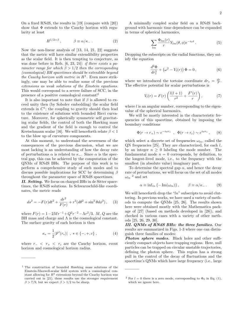
FIG. 1. Lowest lying quasinormal modes for l = 1 andΛM2 = 0.06 (left) and 0.14 (right), as a function of Q/M .The top plots show the imaginary part, with dashed red linescorresponding to purely imaginary modes, and solid blue tocomplex, “PS” modes, whose real part is shown in the lowerplots. The red circles in the top plots indicate the modes ofempty de Sitter at the same Λ, which closely matches the firstimaginary mode here, but lie increasingly less close to thehigher modes. Near the extremal limit of maximal charge,another set of purely imaginary modes (dotted green lines)comes in from −∞ and approaches 0 in the limit. Only afinite number of modes are shown, even though we expectinfinitely many complex and extremal modes in the rangeshown.

|Reω|) [11, 31–33]. For instance, the decay timescale isrelated to the instability timescale of null geodesics nearthe photon sphere. For BHs in de Sitter space, we do finda family of modes which can be traced back to the pho-ton sphere. We refer to them as “photon sphere modes,”or in short “PS” modes. These modes are depicted inblue (solid line) in Figs. 1-3. Different lines correspondto different overtones n; the fundamental mode is deter-mined by the large l limit (and n = 0); we find thatl = 10 or l = 100 provide good approximations of theimaginary parts of the dominating mode; note howeverthat the real parts do not converge when l →∞. Thesemodes are well-described by a WKB approximation, andfor very small cosmological constant they asymptote tothe Schwarzschild BH QNMs [26].

For small values of the cosmological constant, PSmodes are only weakly dependent on the BH charge. Thisis apparent from Fig. 1.

For ΛM2 > 1/9 there is now a nonzero minimal charge,at which r+ = rc. This limit is the charged Nariai BHand is shown as the blue dashed line in Fig. 2. The cor-responding QNMs are also qualitatively different, as seenin Fig. 1. They in fact vanish in this limit, a result thatcan be established by solving the wave equation analyt-ically to obtain (see Ref. [34] for the neutral case, wehave generalized it to charged BHs, see Supplementary

Material)

Im(ω)

κ+= −i

(n+

1

2

). (10)

Note that the results presented here are enough todisprove a conjecture [35] that suggested that α shouldbe equal to min{κ+, κc}. Such possibility is inconsis-tent with (19) and it is also straightforward to find othernon-extremal parameters for which the WKB predictionyields smaller α’s (e.g. for ΛM2 = 0.1 and Q = 0 wehave κ+ = 0.06759, κc = 0.05249, and α = 0.03043).dS modes. Note that solutions with purely imaginaryω exist in pure dS spacetime [36, 37]

ω0,pure dS/κdSc = −il , (11)

ωn 6=0,pure dS/κdSc = −i(l + n+ 1) . (12)

Our second family of modes, the (BH) dS modes, aredeformations of the pure de Sitter modes (12); the dom-inant mode (l = 1, n = 0) is almost identical and highermodes have increasingly larger deformations.

These modes are intriguing, in that they have a sur-prisingly weak dependence on the BH charge and seemto be described by the surface gravity κdSc =

√Λ/3 of

the cosmological horizon of pure de Sitter, as opposedto that of the cosmological horizon in the RNdS BH un-der consideration. This can, in principle, be explainedby the fact that the accelerated expansion of the RNdSspacetimes is also governed by κdSc [38, 39].

This family has been seen in time-evolutions [40] but,to the best of our knowledge, was only recently identifiedin the QNM calculation of neutral BH spacetimes [27].Furthermore, our results indicate that as the BH “disap-pears” (ΛM2 → 0), these modes converge to the exactde Sitter modes (both the eigenvalue and the eigenfunc-tion itself).Near-Extremal modes. Finally, in the limit that theCauchy and event horizon radius approach each other,a third “near extremal” family, labeled as ωNE, domi-nates the dynamics. In the extremal limit this familyapproaches

ωNE = −i(l + n+ 1)κ− = −i(l + n+ 1)κ+ , (13)

independently of Λ, as shown by our numerics. As indi-cated by (13), the dominant mode in this family is thatfor l = 0, this remains true away from extremality.

In the asymptotically flat case, such modes seem tohave been described analytically in Refs. [41–43]. Herewe have shown numerically that such modes exist, andthat they are in fact the limit of a new family of modes. Itis unclear (but see Ref. [42]) if the NE family is a chargedversion of the Zero-Damping-Modes discussed recently inthe context of rotating Kerr BHs [44]. It is also unclear ifthere is any relation between such long lived modes andthe instability of exactly extremal geometries [45, 46].IV. Maximizing β. The dominating modes of the pre-vious three families determine β, shown in Fig. 2. Each

4

βdS

��-�

��-�

��-�

��-�

��-�

�/�

βPS

��-�

��-�

��-�

��-�

��-�

�/�

βNE

�

�

���� ���� ���� ���� �������

���

���

���

���

���

Λ ��

�/�

βdS

��-�

��-�

��-�

��-�

��-�

�/�

βPS

��-�

��-�

��-�

��-�

��-�

�/�

βNE

�

�

���� ���� ���� ���� �������

���

���

���

���

���

Λ ��

�/�

FIG. 2. Parameter space of the RNdS solutions, bounded bya line of extremal solutions of maximal charge where r− = r+on top, and for ΛM2 > 1/9 a line of extremal solutions whererc = r+. In the physical region the value of β is shown. Forsmall ΛM2 the dominant mode is the l = 1 de Sitter mode,shown in shades of red. For larger ΛM2 the dominant modeis the large l complex, PS mode, here showing the l = 100WKB approximated mode in shades of blue. For very largeQ/M the l = 0 extremal mode dominates. The green sliver ontop where the NE mode dominates is merely indicative, thetrue numerical region is too small to be noticeable on thesescales.

family has a region in parameter space where it domi-nates over the other families. The dS family is dominantfor “small” BHs (when ΛM2 . 0.02). In the oppositeregime the PS modes are dominant. Notice that in thelimit of minimal charge β = 0, since κ− remains finitewhile the imaginary parts of QNMs in the PS family ap-proach 0 according to (19) (since κ+ → 0).

More interesting is the other extremal limit, of maxi-mal charge. In Fig. 2, the uppermost contours of the dSand PS families show a region where β > 1/2.

Within this region as the charge is increased even fur-ther, the NE family becomes dominant. In Fig. 2 this isshown merely schematically, as the region is too small toplot on this scale, but it can already be seen in Fig. 1.

To see more clearly how β behaves in the extremal limitwe show 4 more constant ΛM2 slices in Fig. 3. Here onesees clearly how above some value of the charge β >1/2, as dictated by either the de Sitter or the PS family.Increasing the charge further, β would actually divergeif it were up to these two families (ωM approaches aconstant for both families, so ω/κ− diverges). However,the NE family takes over to prevent β from becominglarger than 1. Further details on these modes and on themaximum β are shown in the Supplementary Material.

V. Conclusions. The results in [13, 14] show that thedecay of small perturbations of de Sitter BHs is dictatedby the spectral gap α. At the same time, the linear anal-ysis in [19] and the non-linear analysis in [21] indicatethat the size of β ≡ α/κ− controls the stability of Cauchyhorizons and consequently the fate of the SCC conjecture.Recall that for the dynamics of the Einstein equations,

������ ������ �

�

-���

-��

������ ������ �

������ ������ ��

�

-���

-��

������ ������ �

��(ω

)/κ-

��(ω

)/κ-

�/���� �/����

Λ = � Λ �� = ����

Λ �� = ���� Λ �� = ����

FIG. 3. Dominant modes of different types, showing the(nearly) dominant complex PS mode (blue, solid) at l = 10,the dominant de Sitter mode (red, dotted) at l = 1 and thedominant NE mode (green, dashed) at l = 0. The two dashedvertical lines indicate the points where β ≡ − Im(ω)/κ− =1/2 and where the NE becomes dominant. (Note that thevalue of β is only relevant for Λ > 0.)

and also for the destiny of observers, the blow up of cur-vature (related to β < 1) per se is of little significance: itimplies neither the breakdown of the field equations [47]nor the destruction of macroscopic observers [48]. Infact, a formulation of SCC in those terms is condemnedto overlook relevant physical phenomena like impulsivegravitational waves or the formation of shocks in rela-tivistic fluids. For those and other reasons, the modernformulation of SCC, which we privilege here, makes thestronger request β < 1

2 in order to guarantee the break-down of the field equation at the Cauchy horizon.

Here, by studying (linear) massless scalar fields andsearching through the entire parameter space of subex-tremal and extremal RNdS spacetimes, we find rangesfor which β exceeds 1/2 but, remarkably, it doesn’t seemto be allowed, by the appearance of a new class of “near-extremal” modes, to exceed unity! This opens the per-spective of having Cauchy horizons which, upon pertur-bation, can be seen as singular, by the divergence ofcurvature invariants, but nonetheless maintain enoughregularity as to allow the field equations to determine(classically), in a highly non-unique way, the evolutionof gravitation. This corresponds to a severe failure ofdeterminism in GR that cannot be taken lightly in viewof the importance that a cosmological constant has incosmology and the fact that the pathologic behavior isobserved in parameter ranges which are in loose agree-ment with what one expects from the parameters of someastrophysical BHs 3 [49–51].

3 Astrophysical BHs are expected to be neutral and here we aredealing with charged BHs. This is justified by the standard

5

Acknowledgments. V.C. is indebted to Kinki Univer-sity in Osaka and to the Kobayashi-Maskawa Institute inNagoya for hospitality, while the late stages of this workwere being completed. V.C. and K.D. acknowledge fi-nancial support provided under the European Union’sH2020 ERC Consolidator Grant “Matter and strong-field gravity: New frontiers in Einstein’s theory” grantagreement no. MaGRaTh–646597. Research at Perime-ter Institute is supported by the Government of Canadathrough Industry Canada and by the Province of On-tario through the Ministry of Economic Development &Innovation. J.L.C. acknowledges financial support pro-vided by FCT/Portugal through UID/MAT/04459/2013and grant (GPSEinstein) PTDC/MAT-ANA/1275/2014.A.J. was supported by the Netherlands Organisation forScientific Research (NWO) under VIDI grant 680-47-518,

and the Delta-Institute for Theoretical Physics (D- ITP)that is funded by the Dutch Ministry of Education, Cul-ture and Science (OCW). This project has received fund-ing from the European Union’s Horizon 2020 researchand innovation programme under the Marie Sklodowska-Curie grant agreement No 690904. Part of this researchwas conducted during the time P.H. served as a ClayResearch Fellow; P.H. also acknowledges support fromthe Miller Institute at UC Berkeley. The authors wouldlike to acknowledge networking support by the COSTAction GWverse CA16104. The authors thankfully ac-knowledge the computer resources, technical expertiseand assistance provided by Sergio Almeida at CEN-TRA/IST. Computations were performed at the cluster“Baltasar-Sete-Sois”, and supported by the MaGRaTh–646597 ERC Consolidator Grant.

[1] R. H. Price, Phys. Rev. D5, 2419 (1972).[2] M. Dafermos, I. Rodnianski, and Y. Shlapentokh-

Rothman, (2014), arXiv:1402.7034 [gr-qc].[3] Y. Angelopoulos, S. Aretakis, and D. Gajic, (2016),

arXiv:1612.01566 [math.AP].[4] E. Poisson and W. Israel, Phys. Rev. D41, 1796 (1990).[5] M. Dafermos, Commun. Pure Appl. Math. 58, 0445

(2005), arXiv:gr-qc/0307013 [gr-qc].[6] M. Dafermos, Commun. Math. Phys. 332, 729 (2014),

arXiv:1201.1797 [gr-qc].[7] J. Luk and S.-J. Oh, Preprint, arXiv:1702.05715 (2017).[8] J. Luk and S.-J. Oh, Preprint, arXiv:1702.05716 (2017).[9] S. Barreto and M. Zworski, Math. Res. Lett. 4, 103

(1997).[10] J.-F. Bony and D. Hafner, Communications in Mathe-

matical Physics 282, 697 (2008).[11] S. Dyatlov, Annales Henri Poincare 13, 1101 (2012),

arXiv:1101.1260 [math.AP].[12] S. Dyatlov, Commun. Math. Phys. 335, 1445 (2015),

arXiv:1305.1723 [gr-qc].[13] P. Hintz and A. Vasy, (2016), arXiv:1606.04014

[math.DG].[14] P. Hintz, Preprint, arXiv:1612.04489 (2016).[15] A. Ori, Phys. Rev. D61, 064016 (2000).[16] J. L. Costa, P. M. Girao, J. Natario, and J. D. Silva,

Ann. PDE 3, 8 (2017), arXiv:1406.7261 [gr-qc].[17] J. Earman, Oxford Univ. Pr (1995).[18] D. Christodoulou (2008) pp. 24–34, arXiv:0805.3880 [gr-

qc].[19] P. Hintz and A. Vasy, J. Math. Phys. 58, 081509 (2017),

arXiv:1512.08004 [math.AP].[20] J. L. Costa and A. T. Franzen, Ann. Henri Poincare 18,

3371 (2017), arXiv:1607.01018 [gr-qc].[21] J. L. Costa, P. M. Girao, J. Natario, and J. D. Silva,

(2017), arXiv:1707.08975 [gr-qc].[22] M. Dafermos and J. Luk, (2017), arXiv:1710.01722 [gr-

qc].

charge/angular momentum analogy, where near-extremal chargecorresponds to fast rotating BHs.

[23] K. Maeda, T. Torii, and M. Narita, Phys. Rev. D61,024020 (2000), arXiv:gr-qc/9908007 [gr-qc].

[24] J. L. Costa, P. M. Girao, J. Natario, and J. D. Silva,Class. Quant. Grav. 32, 015017 (2015), arXiv:1406.7245[gr-qc].

[25] E. Berti, V. Cardoso, and A. O. Starinets, Class. Quant.Grav. 26, 163001 (2009), arXiv:0905.2975 [gr-qc].

[26] https://centra.tecnico.ulisboa.pt/network/grit/

files/.[27] A. Jansen, (2017), arXiv:1709.09178 [gr-qc].[28] O. J. C. Dias, P. Figueras, R. Monteiro, H. S. Reall,

and J. E. Santos, JHEP 05, 076 (2010), arXiv:1001.4527[hep-th].

[29] K. Lin and W.-L. Qian, ArXiv e-prints (2016),arXiv:1609.05948 [math.NA].

[30] S. Iyer and C. M. Will, Phys. Rev. D35, 3621 (1987).[31] V. Cardoso and P. Pani, Nat. Astron. 1, 586 (2017),

arXiv:1707.03021 [gr-qc].[32] V. Cardoso, A. S. Miranda, E. Berti, H. Witek,

and V. T. Zanchin, Phys. Rev. D79, 064016 (2009),arXiv:0812.1806 [hep-th].

[33] S. Dyatlov and M. Zworski, Phys. Rev. D 88, 084037(2013).

[34] V. Cardoso and J. P. S. Lemos, Phys. Rev. D67, 084020(2003), arXiv:gr-qc/0301078 [gr-qc].

[35] P. R. Brady, I. G. Moss, and R. C. Myers, PhysicalReview Letters 80, 3432 (1998).

[36] A. Lopez-Ortega, Gen. Rel. Grav. 44, 2387 (2012),arXiv:1207.6791 [gr-qc].

[37] A. Vasy, Advances in Mathematics 223, 49 (2010).[38] D. R. Brill and S. A. Hayward, Class. Quant. Grav. 11,

359 (1994), arXiv:gr-qc/9304007 [gr-qc].[39] A. D. Rendall, Annales Henri Poincare 5, 1041 (2004),

arXiv:gr-qc/0312020 [gr-qc].[40] P. R. Brady, C. M. Chambers, W. G. Laarakkers, and

E. Poisson, Phys. Rev. D60, 064003 (1999), arXiv:gr-qc/9902010 [gr-qc].

[41] Y.-W. Kim, Y. S. Myung, and Y.-J. Park, Eur. Phys. J.C73, 2440 (2013), arXiv:1205.3701 [hep-th].

[42] A. Zimmerman and Z. Mark, Phys. Rev. D93, 044033(2016), [Erratum: Phys. Rev.D93,no.8,089905(2016)],arXiv:1512.02247 [gr-qc].

6

[43] S. Hod, Eur. Phys. J. C77, 351 (2017), arXiv:1705.04726[hep-th].

[44] M. Richartz, C. A. R. Herdeiro, and E. Berti, Phys. Rev.D96, 044034 (2017), arXiv:1706.01112 [gr-qc].

[45] S. Aretakis, Adv. Theor. Math. Phys. 19, 507 (2015),arXiv:1206.6598 [gr-qc].

[46] M. Casals, S. E. Gralla, and P. Zimmerman, Phys. Rev.D94, 064003 (2016), arXiv:1606.08505 [gr-qc].

[47] S. Klainerman, I. Rodnianski, and J. Szeftel, Invent.Math. 202, 91 (2015), arXiv:1204.1767 [math.AP].

[48] A. Ori, Phys. Rev. Lett. 67, 789 (1991).[49] L. W. Brenneman, C. S. Reynolds, M. A. Nowak,

R. C. Reis, M. Trippe, A. C. Fabian, K. Iwasawa,J. C. Lee, J. M. Miller, R. F. Mushotzky, K. Nan-dra, and M. Volonteri, Astrophys. J. 736, 103 (2011),arXiv:1104.1172 [astro-ph.HE].

[50] M. Middleton, “Black hole spin: Theory and observa-tion,” in Astrophysics of Black Holes: From Fundamen-tal Aspects to Latest Developments, edited by C. Bambi(Springer Berlin Heidelberg, Berlin, Heidelberg, 2016)pp. 99–151.

[51] G. Risaliti, F. Harrison, K. Madsen, D. Walton, S. Boggs,F. Christensen, W. Craig, B. Grefenstette, C. Hailey,E. Nardini, et al., Nature 494, 449 (2013).

7

Supplementary MaterialThe eigenfunctions The difference between PS, dS andNE modes is also apparent from the eigenfunction itself.It is useful to define a re-scaled function φ(r) as,

Φ(r) = (r − r+)−iω/(2κ+)φ(r)(rc − r)−iω/(2κc) . (14)

The conditions on φ(r) are that it approaches a con-stant as r → r+, rc, Figure 4 shows the behavior of φ

for different modes, for a specific set of RNdS parame-ters. Although not apparent, there is structure close tothe photon sphere for the PS eigenfunction.

Analytic solutions for rc = r+ In the limit rc = r+,the limit of minimal charge for ΛM2 ≥ 1/9, the quasi-normal modes can be found analytically. In this limit,equation (6) with potential (7), written in the coordinatex = (r − r+)/(rc − r+), becomes

(4r+x(1− x)

3− 2r+l(l + 1) + λ2

)φ(x) + 4x(1− x)(1− 2x)φ′(x) + 4x2(1− x)2φ′′(x) = 0 (15)

where we defined λ ≡ ω/κ+ and we have set M = 1,which can be restored in the end by dimensional analysis.

This equation has the solutions

φ(x) = c1Piλα (2x− 1) + c2Q

iλα (2x− 1) , (16)

where P,Q are the Legendre P and Q functions, and

α =1

2

(−1 +

√1− 2r+

r+ − 3/2l(l + 1)

). (17)

Now, analysis of the asymptotic behavior near x = 0and x = 1 shows that we can only satisfy the “outgoing”boundary conditions [25] when c2 = 0 and λ is eitherλ = −i(α+ n), or λ = −i(n+ 1− α). These combine togive

ω

κ+= ±1

2

√−1 + l(l + 1)

2r+r+ − 3/2

− i(n+

1

2

), (18)

Restoring units we obtain,

ω

κ+= ±1

2

√−1 + 2l(l + 1)Υ− i

(n+

1

2

), (19)

Υ =γ2 + 21/3ΛM2

γ2 + (21/3 − 3× 2−1/3γ)ΛM2,

γ =(−3(ΛM2)2 + (ΛM2)3/2

√(9ΛM2 − 2)

)1/3.

The argument of the square root in (19) is positive. Theimaginary part of these frequencies is exactly the sameas that of the neutral Nariai BH [34]. The real part isdifferent and now depends also on Λ, but asymptotes tothe previous result for Q = 0 (i.e., Λ = 1/9), as it should.It is an interesting feature that when ΛM2 → 2/9, Υ, andtherefore the real part of ω/κ+, diverges.Searching for long-lived modes Here we address thequestion whether there might be a more slowly decayingmode that we have missed and could save SCC. If sucha mode exists, it would be highly unlikely to be partof the three families we found, since we can follow theircontinuous change as the BH parameters are varied, as

��� ��� ��� ��� ��� ���-���

-���

���

���

���

�

ϕ(�)

FIG. 4. Scalar wavefunctions φ(x) (defined in Eq. (14), withx = (r − r+)/(rc − r+)) of the dominant mode of each ofthe three families, at ΛM2 = 0.02 and Q/Qmax ≈ 0.9966,as indicated in the top right of Fig. (3). Shown are thenear extremal mode with ωNE/κ− = −0.87005i (for l = 0,green dotted line), the dS mode with ωdS/κ− = −0.87043i(for l = 1, red dashed line), and the complex mode withωC/κ− = 26.448 − 0.89101i (for l = 10, blue solid and dash-dotted line for real and imaginary parts). The solid verticalblack line indicates the light ring.

shown in the figures. Furthermore, the known modesin the limiting cases are all accounted for, and we neverobserved any mode crossings for given family and angularmomentum l.

It is theoretically possible, though also very unlikely,that there is a fourth family (with anywhere between asingle and infinitely many members) that we have missed.

Typically, smaller eigenvalues are found more easilythan larger eigenvalues, making it more unlikely to missthe dominant mode. It could be however that the corre-sponding eigenfunction is either very sharply peaked orhighly oscillatory, in which cases it would require a largenumber of grid points to be resolved accurately enough.This again decreases the possibility that we have missedsomething. We will rule out this last scenario, as bestas we can numerically, as follows. We pick a representa-

8

l ω0/κ−

0 -0.8539013779 i(61)

1 3.2426164126 - 0.7958326323 i(67)

( -1.5003853731 i(64))

2 5.4796067815 - 0.7754179185 i(69)

3 7.7016152057 - 0.7699348317 i(70)

4 9.9181960834 - 0.7676996545 i(73)

5 12.1322536641 - 0.7665731858 i(75)

10 23.1897597770 - 0.7649242108 i(80)

100 222.0602900249 - 0.7643094446 i(82)

TABLE I. The dominant quasinormal modes for a rangeof angular momenta l, in units of the surface gravity ofthe Cauchy horizon, for the BH with ΛM2 = 0.06 andQ/Qmax = 0.996. The bold, underlined modes at l = 0, 1and 10 are the dominant modes for the near-extremal-, deSitter- and photon sphere modes respectively, as seen also inthe bottom left of Fig. 3. Note that the de Sitter mode is sub-dominant even for fixed l = 1, and the photon sphere mode atl = 10 is only dominant to very good approximation, the truedominant mode being that with l→∞. Numbers in bracketsindicate the number of agreed digits in the computations withgrid size and precision (N, p) = (400, 200) and (450, 225).

tive BH for which β > 1/2, indicating violation of SCC,

namely ΛM2 = 0.06 and Q/Qmax = 0.996. For these BHparameters we compute the QNMs for various angularmomenta l as shown in Table I. There is no new QNMthat is more dominant than those found before, exceptas expected the l = 100 photon sphere mode, but notsignificantly, note the extremely rapid convergence withincreasing l.

The main method we use essentially discretizes theequation and rearranges it into a generalized eigenvalueequation, whose eigenvalues are the QNMs (see [27] formore details). This has two technical parameters, thenumber of grid points N and the precision p (numberof digits) used in the computation. To be sure that theobtained results are not numerical artefacts one has torepeat the computation at different (N, p) and test forcovergence, which we have done for all results shown.

The computation here was done at even higher accu-racy than in the main results, with (N, p) = (400, 200)and (450, 225). The most we used previously was(300, 150) and (350, 175) (near extremality, away fromextremality a much lower accuracy usually suffices). Thenumber in brackets behind each mode in Table I is thenumber of digits that agrees between the computationsat these two accuracies.

We checked that even before testing for convergence,there are no modes with imaginary part smaller (in ab-solute sense) than shown in Table I. This confirms ourresults with as much certainty as one can reasonably ex-pect from a numerical result.