Quasiparticle Interference, quasiparticle interactions and the

origin of the charge density-wave in 2H-NbSe2

C. J. Arguello1, E. P. Rosenthal1, E. F. Andrade1, W. Jin2, P. C. Yeh2, N. Zaki3, S. Jia4, R.

J. Cava4, R. M. Fernandes5, A. J. Millis1, T. Valla6, R. M. Osgood Jr.3,4, A. N. Pasupathy1

1. Department of Physics, Columbia University, NY, NY, 10027

2. Department of Applied Physics and Applied Math,

Columbia University, NY, NY, 10027

3. Department of Electrical Engineering,

Columbia University, NY, NY, 10027

4. Department of Chemistry, Princeton University, Princeton NJ 08540

5. School of Physics and Astronomy,

University of Minnesota, Minneapolis,

MN 55455 6. Brookhaven National Laboratory, Upton NY

(Dated: August 26, 2014)

Abstract

We show that a small number of intentionally introduced defects can be used as a spectroscopic

tool to amplify quasiparticle interference in 2H-NbSe2, that we measure by scanning tunneling

spectroscopic imaging. We show from the momentum and energy dependence of the quasiparticle

interference that Fermi surface nesting is inconsequential to charge density wave formation in

2H-NbSe2. We demonstrate that by combining quasiparticle interference data with additional

knowledge of the quasiparticle band structure from angle resolved photoemission measurements,

one can extract the wavevector and energy dependence of the important electronic scattering

processes thereby obtaining direct information both about the fermiology and the interactions.

In 2H-NbSe2, we use this combination to show that the important near-Fermi-surface electronic

physics is dominated by the coupling of the quasiparticles to soft mode phonons at a wave vector

different from the CDW ordering wave vector.

1

BNL-107408-2015-JA

In many complex materials including the two dimensional cuprates, the pnictides, and

the dichalcogenides the electronic ground state may spontaneously break the translational

symmetry of the lattice. Such density wave ordering can arise from Fermi surface nesting,

from strong electron-electron interactions, or from interactions between the electrons and

other degrees of freedom in the material, such as phonons. The driving force behind the for-

mation of the spatially ordered states and the relationship of these states to other electronic

phases such as superconductivity remains hotly debated.

Scanning tunneling spectroscopy (STS) has emerged as a powerful technique for probing

the electronic properties of such ordered states at the nanoscale [1–3] due to its high energy

and spatial resolution. The position dependence of the current I-voltage V characteristics

measured in STS experiments maps the energy dependent local density of states ρ(r, E) [4, 5].

Correlations between the ρ(r, E) at different points at a given energy reveal the pattern of

standing waves produced when electrons scatter off of impurities [6]. These quasiparticle

interference (QPI) features may be analyzed to reveal information about the momentum

space structure of the electronic states [7]. The intensity of the QPI signals as a function

of energy and momentum also contains information about the electronic interactions in the

material [8, 9].

In this work, we take the ideas further, showing how impurities can be used intentionally

to enhance QPI signals in STS experiments and how the combination of the enhanced QPI

signals with electronic spectroscopic information available in angle-resolved photoemission

(ARPES) measurements can be used to gain insight into the physics underlying electronic

symmetry breaking and quasiparticle interactions. By observing the electronic response to

the addition of dilute, weak impurities to the charge density wave material 2H-NbSe2 we

directly measure the dominant electronic scattering channels. We show conclusively that

Fermi surface nesting does not drive CDW formation and that the dominant quasiparticle

scattering arises from soft-mode phonons.

Our theoretical analysis begins from a standard relation between the current-voltage

characteristic dIdV

at position r and voltage difference V = E and the electron Green’s

function G, valid if the density of states in the tip used in the STS experiment is only

weakly energy dependent

dI(r, E)

dV= Tr

[Mtun (G(r, r, E − iδ)−G(r, r, E + iδ))

2πi

](1)

2

Here M is a combination of the tunneling matrix element and wave functions (see supple-

mentary material); M and G are matrices in the space of band indices.

To calculate the changes in dI/dV induced by impurities we observe that in the presence

of a single impurity placed at position Ra the electron Green’s function is changed from the

pure system form G to G given by

G(r, r′, E) = G(r− r′, E) + (2)ˆdr1dr2G(r− r1, E)T(r1 −Ra, r2 −Ra, E)G(r2 − r′, E)

Here T(r, r′, E) is the T-matrix describing electron-impurity scattering as renormalized by

electron-electron interactions. It is a matrix in the space of band indices, and we suppress

spin indices, which play no role in our considerations.

Assuming (see supplementary material) that M is structureless (couples all band indices

equally), Fourier transforming and assuming that interference between different impurities

is not important gives for the impurity-induced change in the tunneling current

δdI(k, E)

dV=

(1

v

∑a

eik·Ra

)Φk(E − iδ)− Φk(E + iδ)

2πi(3)

with v the volume of the systems and the scattering function of complex argument z given

in the band basis in which G is diagonal as

Φk(z) =∑nm

ˆGn

p(z)T nmp,p+k(z)Gm

p+k(z)dp (4)

At this stage no assumption has been made about interactions.

From Eq. 3 we see that structure in δdI(k, E)/dV can arise from structure in the com-

bination GpGp+k of electron propagators (Fermi surface nesting) or from structure in the

T-matrix, the latter arising either from properties of the impurity or from interactions

involving the scattered electrons. Combining an STS measurement with an independent

determination of G (for example by ARPES) allows the two physical processes to be distin-

guished. However, a direct analysis of Eq. 3 requires precise measurement of the positions

of all of the impurities so that the∑

a eik·Ra factor can be divided out. This is impractical

at present, so we focus on |δdI(k, E)/dV | where for dilute randomly placed impurities the

prefactor can be replaced by the square root of the impurity density. Eq. 3 can be further

simplified if one assumes that the T matrix depends primarily on the momentum transfer k

3

and has negligible imaginary part (i.e. scattering phase shift near 0 or π). Such an assump-

tion is particularly appropriate when the scattering arises from weakly scattering uncharged

point impurities. We find∣∣∣∣δdI(k, E)

dV

∣∣∣∣ =√nimp

∣∣∣∣∣∑nm

Bnm(k, E)T nmk (E)

∣∣∣∣∣ (5)

with

Bnm(k, E) =∑p

Gnp(E − iδ)Gm

p+k(E − iδ)− (δ ↔ −δ)2πi

(6)

An integral of B over the occupied states yields the components of the noninteracting (Lind-

hard) susceptibility (see supplementary material)

χnm0 (k) ∝

ˆ ∞−∞

dE

πf(E) (Bnm(k, E) +Bmn(k, E)) (7)

where f is the Fermi function. This observation permits an interesting analysis. If the

impurity scattering potential Vimp is structureless and weak, a measurement of the QPI

then directly yields the Lindhard susceptiblity. Conversely, if the impurities are known to

be weak, differences between the measured QPI intensity and the Lindhard susceptibility

reveal the effects of interactions, which appear formally as a “vertex correction” of the basic

impurity-quasiparticle scattering amplitude Vimp (see supplementary material).

We apply these concepts to 2H-NbSe2, a quasi-2D transition metal dichalcogenide that

displays a charge density wave (CDW) phase transition below TCDW≈33 K[10–12]. The

physics of this ordered state is still under debate. While some experiments point to an

important role of Fermi surface (FS) nesting [13, 14], perhaps accompanied by a van Hove

singularity[15, 16], an alternative scenario argues that the nesting of the FS is not strong

enough to produce the CDW instability [17, 18], and proposes that a strong electron-phonon

coupling [19, 20] is responsible. ARPES experiments do not detect a strong effect of the

CDW order on the near-FS states.

No signatures of QPI have been detected in previous STS studies of NbSe2, presumably

due to the lack of sufficient scattering centers in the pristine material. To enhance the

QPI signal we introduced dilute sulfur doping to pristine NbSe2 (NbSe(2−x)Sx). S and Se are

isovalent atoms, so no charge doping arises from the substitution. Furthermore, the similarity

of the calculated band structures of NbSe2 and NbS2 shows that the bare scattering potential

induced by the substitution Se→ S is weak. We have estimated the S-defect concentration

4

a

d

c

b10

-10

Z(pm)

5

-5

FFT Power (a. u.)

0

6

10 nm

3.5nm

b

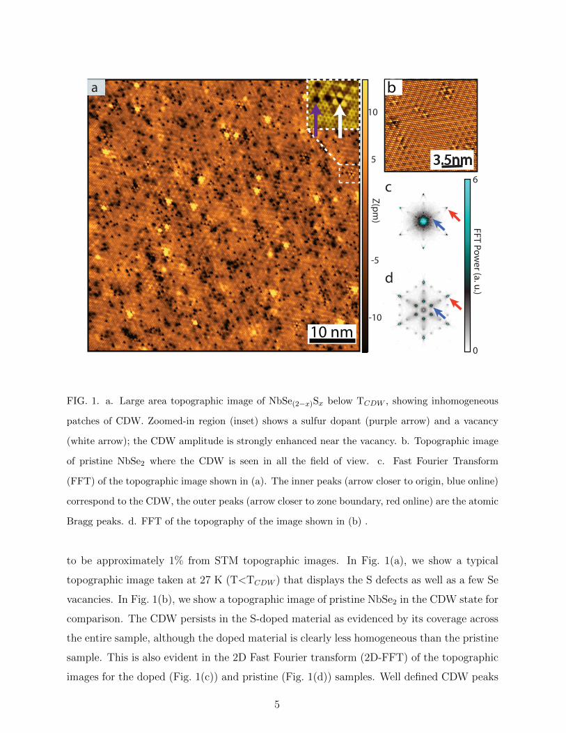
FIG. 1. a. Large area topographic image of NbSe(2−x)Sx below TCDW , showing inhomogeneous

patches of CDW. Zoomed-in region (inset) shows a sulfur dopant (purple arrow) and a vacancy

(white arrow); the CDW amplitude is strongly enhanced near the vacancy. b. Topographic image

of pristine NbSe2 where the CDW is seen in all the field of view. c. Fast Fourier Transform

(FFT) of the topographic image shown in (a). The inner peaks (arrow closer to origin, blue online)

correspond to the CDW, the outer peaks (arrow closer to zone boundary, red online) are the atomic

Bragg peaks. d. FFT of the topography of the image shown in (b) .

to be approximately 1% from STM topographic images. In Fig. 1(a), we show a typical

topographic image taken at 27 K (T<TCDW ) that displays the S defects as well as a few Se

vacancies. In Fig. 1(b), we show a topographic image of pristine NbSe2 in the CDW state for

comparison. The CDW persists in the S-doped material as evidenced by its coverage across

the entire sample, although the doped material is clearly less homogeneous than the pristine

sample. This is also evident in the 2D Fast Fourier transform (2D-FFT) of the topographic

images for the doped (Fig. 1(c)) and pristine (Fig. 1(d)) samples. Well defined CDW peaks

5

a

5 nm

-110meV b

-110 meV -50 meV

+50 meV +110 meV

CDW

QPI M K

70

0

nS

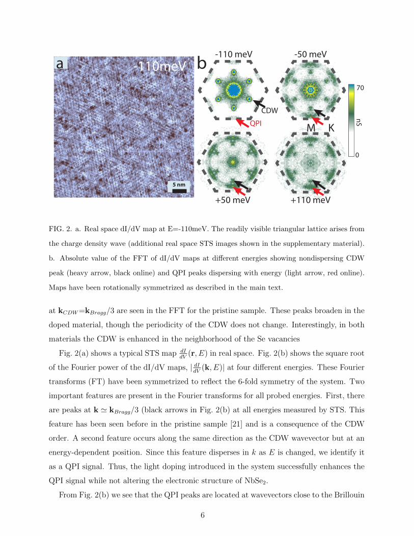
FIG. 2. a. Real space dI/dV map at E=-110meV. The readily visible triangular lattice arises from

the charge density wave (additional real space STS images shown in the supplementary material).

b. Absolute value of the FFT of dI/dV maps at different energies showing nondispersing CDW

peak (heavy arrow, black online) and QPI peaks dispersing with energy (light arrow, red online).

Maps have been rotationally symmetrized as described in the main text.

at kCDW=kBragg/3 are seen in the FFT for the pristine sample. These peaks broaden in the

doped material, though the periodicity of the CDW does not change. Interestingly, in both

materials the CDW is enhanced in the neighborhood of the Se vacancies

Fig. 2(a) shows a typical STS map dIdV

(r, E) in real space. Fig. 2(b) shows the square root

of the Fourier power of the dI/dV maps, | dIdV

(k, E)| at four different energies. These Fourier

transforms (FT) have been symmetrized to reflect the 6-fold symmetry of the system. Two

important features are present in the Fourier transforms for all probed energies. First, there

are peaks at k ' kBragg/3 (black arrows in Fig. 2(b) at all energies measured by STS. This

feature has been seen before in the pristine sample [21] and is a consequence of the CDW

order. A second feature occurs along the same direction as the CDW wavevector but at an

energy-dependent position. Since this feature disperses in k as E is changed, we identify it

as a QPI signal. Thus, the light doping introduced in the system successfully enhances the

QPI signal while not altering the electronic structure of NbSe2.

From Fig. 2(b) we see that the QPI peaks are located at wavevectors close to the Brillouin

6

zone edge for E=-110meV and move towards the zone center with increasing energy. We

see however that for all energies presented in this paper the QPI peaks remain far from the

CDW wave vector. This is illustrated more clearly in Fig. 3(a) which presents a line-cut of

the STS data along the Γ−M direction for each one of the energy slices of the STS maps.

At the Fermi energy, the QPI signal is separated from the CDW signal by ∆k ' 13kCDW .

Extrapolation to higher energies suggests that kQPI would reach kCDW only at E & 300meV

above the Fermi level.

Combining ARPES and STS measurements allows us to extract important additional

information about the nature of scattering near the Fermi level in the CDW state of NbSe2.

Representative ARPES measurements are presented in Fig. 3(b). Comparison to similar

data obtained on the pristine material [14, 22] revealed no significant changes in the band

dispersion, further confirming that study of the lightly S doped system reveals information

relevant to pristine NbSe2. We fit our ARPES measurements in Fig. 3(b) to a two-band, five

nearest-neighbor, tight-binding model similar to the one presented in Ref. 23 (see supple-

mentary materials for details). This fit captures the primarily two-dimensional Nb-derived

q/QBragg

Energ

y (

meV

)

0 0.1 0.2 0.3 0.4 0.5

150

100

50

0

−50

−100

−150

Kcdw QPI

∆k

High

Low

K M K

ba

FIG. 3. a. Line-cut of the dI/dV maps in Fourier space along the Γ−M direction. The dashed lines

are guides for the eye highlighting the positions of the CDW ordering vector and the quasiparticle

dispersion while the heavy line and shading (pink online) highlights the separation between the QPI

intensity and the CDW wavevector at the Fermi energy. (b) ARPES line-cut along the K−M −K

direction. The dotted line is the tight-binding fit to the data

7

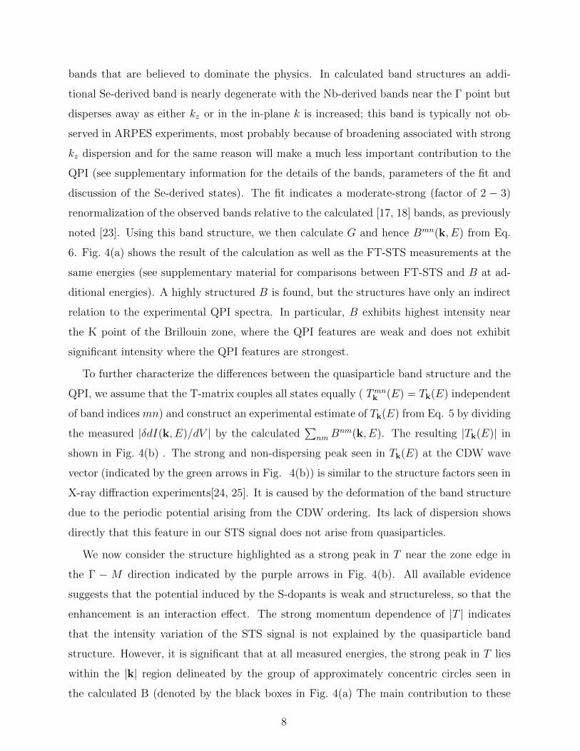
bands that are believed to dominate the physics. In calculated band structures an addi-

tional Se-derived band is nearly degenerate with the Nb-derived bands near the Γ point but

disperses away as either kz or in the in-plane k is increased; this band is typically not ob-

served in ARPES experiments, most probably because of broadening associated with strong

kz dispersion and for the same reason will make a much less important contribution to the

QPI (see supplementary information for the details of the bands, parameters of the fit and

discussion of the Se-derived states). The fit indicates a moderate-strong (factor of 2 − 3)

renormalization of the observed bands relative to the calculated [17, 18] bands, as previously

noted [23]. Using this band structure, we then calculate G and hence Bmn(k, E) from Eq.

6. Fig. 4(a) shows the result of the calculation as well as the FT-STS measurements at the

same energies (see supplementary material for comparisons between FT-STS and B at ad-

ditional energies). A highly structured B is found, but the structures have only an indirect

relation to the experimental QPI spectra. In particular, B exhibits highest intensity near

the K point of the Brillouin zone, where the QPI features are weak and does not exhibit

significant intensity where the QPI features are strongest.

To further characterize the differences between the quasiparticle band structure and the

QPI, we assume that the T-matrix couples all states equally ( Tmnk (E) = Tk(E) independent

of band indices mn) and construct an experimental estimate of Tk(E) from Eq. 5 by dividing

the measured |δdI(k, E)/dV | by the calculated∑

nmBnm(k, E). The resulting |Tk(E)| in

shown in Fig. 4(b) . The strong and non-dispersing peak seen in Tk(E) at the CDW wave

vector (indicated by the green arrows in Fig. 4(b)) is similar to the structure factors seen in

X-ray diffraction experiments[24, 25]. It is caused by the deformation of the band structure

due to the periodic potential arising from the CDW ordering. Its lack of dispersion shows

directly that this feature in our STS signal does not arise from quasiparticles.

We now consider the structure highlighted as a strong peak in T near the zone edge in

the Γ − M direction indicated by the purple arrows in Fig. 4(b). All available evidence

suggests that the potential induced by the S-dopants is weak and structureless, so that the

enhancement is an interaction effect. The strong momentum dependence of |T | indicates

that the intensity variation of the STS signal is not explained by the quasiparticle band

structure. However, it is significant that at all measured energies, the strong peak in T lies

within the |k| region delineated by the group of approximately concentric circles seen in

the calculated B (denoted by the black boxes in Fig. 4(a) The main contribution to these

8

circles arises from 2kF backscattering across each of the Fermi surfaces. This suggests that

the observed QPI arises from an enhancement of backscattering [26] by a strongly direction-

dependent interaction [27]. Available calculations [19, 28] suggest that soft acoustic phonons

with wavevector along the Γ−M direction are strongly coupled to electrons for a wide range

of |k|. By contrast the high intensity regions in B near the K point arise from approximate

nesting of the Fermi surfaces centered at Γ and K; that these are not seen in the measured

QPI again confirms that nesting is not enhanced by interactions and is not important in this

material. We therefore propose that the observed QPI signal arises from a renormalization

of a structureless impurity potential by the electron-phonon interaction.

In summary, we used dilute doping of NbSe2 with isovalent S atoms to enhance the QPI

signal and, by combining STS and ARPES measurements were able to show that the QPI

signal measures more than just the fermiology of the material. We were able to confirm

that the CDW does not arise from Fermi-surface nesting and we identified an important

quasiparticle interaction, most likely of electron-phonon origin. Our approach reveals that

the response to deliberately-induced dopants is an important spectroscopy of electronic

behavior. We expect it can be extended to many other systems.

ACKNOWLEDGMENTS

Acknowledgements:

This work was supported by the National Science Foundation (NSF) under grant DMR-

1056527 (ER, ANP) and by the Materials Interdisciplinary Research Team grant number

DMR-1122594 (ANP,AJM). Salary support was also provided by the U.S. Department of

Energy under Contract No. DE-FG 02-04-ER-46157 (W.J., P.C.Y., N.Z., and R.M.O.) and

DE-SC0012336 (RMF). ARPES research carried out at National Synchrotron Light Source,

Brookhaven National Laboratory is supported by the U.S. Department of Energy, Office of

Basic Energy Sciences (DOE-BES), under the Contract No. DE-AC02-98CH10886. The

crystal growth work at Princeton University was funded by DOE-BES grant DE -FG02-

98ER45706. AJM acknowledges the hospitality of the Aspen Center for Physics (supported

9

a -50meV 50meV

b -100meV 100meV 0meV

HighLow

Low

High

FIG. 4. a. Absolute value of FFT of experimental (left half of image ) and theoretical (right

half of image) dI/dV map at E=-50meV (left image) and E=50meV (right image). Theoretical

images calculated as∑

mnBmn (k, E) using Eq. 6 with tight-binding model bands obtained from

fits to ARPES measurements as described in the supplementary material. The dotted line is the

edge of the first Brillouin zone. The black boxes indicate the areas in k space where the T-matrix

is strongly peaked. b. |Tk(E)| calculated from the STS data using eq. 5 for -100meV (left),

Fermi energy (center) and 100meV (right). The green arrow points to the position of the CDW

wavevector, the purple arrow points to the dispersing feature in the T-matrix.

10

by NSF Grant 1066293) for hospitality during the conception and writing of this manuscript.

[1] Y. Kohsaka, C. Taylor, K. Fujita, A. Schmidt, C. Lupien, T. Hanaguri,

M. Azuma, M. Takano, H. Eisaki, H. Takagi, et al., Science 315, 1380 (2007),

http://www.sciencemag.org/content/315/5817/1380.full.pdf, URL http://www.sciencemag.

org/content/315/5817/1380.abstract.

[2] M. Vershinin, S. Misra, S. Ono, Y. Abe, Y. Ando, and A. Yazdani, Science 303, 1995 (2004),

http://www.sciencemag.org/content/303/5666/1995.full.pdf, URL http://www.sciencemag.

org/content/303/5666/1995.abstract.

[3] W. D. Wise, M. C. Boyer, K. Chatterjee, T. Kondo, T. Takeuchi, H. Ikuta, Y. Wang, and

E. W. Hudson, Nat Phys 4, 696 (2008), URL http://dx.doi.org/10.1038/nphys1021.

[4] J. Tersoff and D. R. Hamann, Phys. Rev. B 31, 805 (1985), URL http://link.aps.org/

doi/10.1103/PhysRevB.31.805.

[5] J. Li, W.-D. Schneider, and R. Berndt, Phys. Rev. B 56, 7656 (1997), URL http://link.

aps.org/doi/10.1103/PhysRevB.56.7656.

[6] M. F. Crommie, C. P. Lutz, and D. M. Eigler, Nature 363, 524 (1993), cited

By (since 1996):691, URL http://www.nature.com/nature/journal/v363/n6429/abs/

363524a0.html.

[7] K. McElroy, R. W. Simmonds, J. E. Hoffman, D. . Lee, J. Orenstein, H. Eisaki, S. Uchida, and

J. C. Davis, Nature 422, 592 (2003), cited By (since 1996):277, URL http://www.nature.

com/nature/journal/v422/n6932/full/nature01496.html.

[8] S. A. Kivelson, I. P. Bindloss, E. Fradkin, V. Oganesyan, J. M. Tranquada, A. Kapitulnik,

and C. Howald, Rev. Mod. Phys. 75, 1201 (2003), URL http://link.aps.org/doi/10.1103/

RevModPhys.75.1201.

[9] Y. B. Kim and A. J. Millis, Phys. Rev. B 67, 085102 (2003), URL http://link.aps.org/

doi/10.1103/PhysRevB.67.085102.

[10] D. E. Moncton, J. D. Axe, and F. J. DiSalvo, Phys. Rev. Lett. 34, 734 (1975), URL http:

//link.aps.org/doi/10.1103/PhysRevLett.34.734.

[11] J. A. Wilson, F. J. di Salvo, and S. Mahajan, Advances in Physics 24, 117 (1975).

[12] R. Coleman, B. Giambattista, P. Hansma, A. Johnson, W. McNairy, and C. Slough, Advances

11

in Physics 37, 559 (1988), http://dx.doi.org/10.1080/00018738800101439, URL http://dx.

doi.org/10.1080/00018738800101439.

[13] T. Straub, T. Finteis, R. Claessen, P. Steiner, S. Hufner, P. Blaha, C. S. Oglesby, and

E. Bucher, Phys. Rev. Lett. 82, 4504 (1999), URL http://link.aps.org/doi/10.1103/

PhysRevLett.82.4504.

[14] S. V. Borisenko, A. A. Kordyuk, V. B. Zabolotnyy, D. S. Inosov, D. Evtushinsky, B. Buchner,

A. N. Yaresko, A. Varykhalov, R. Follath, W. Eberhardt, et al., Phys. Rev. Lett. 102, 166402

(2009), URL http://link.aps.org/doi/10.1103/PhysRevLett.102.166402.

[15] T. M. Rice and G. K. Scott, Phys. Rev. Lett. 35, 120 (1975), URL http://link.aps.org/

doi/10.1103/PhysRevLett.35.120.

[16] W. C. Tonjes, V. A. Greanya, R. Liu, C. G. Olson, and P. Molinie, Phys. Rev. B 63, 235101

(2001), URL http://link.aps.org/doi/10.1103/PhysRevB.63.235101.

[17] K. Rossnagel, O. Seifarth, L. Kipp, M. Skibowski, D. Voß, P. Kruger, A. Mazur, and

J. Pollmann, Phys. Rev. B 64, 235119 (2001), URL http://link.aps.org/doi/10.1103/

PhysRevB.64.235119.

[18] M. D. Johannes, I. I. Mazin, and C. A. Howells, Phys. Rev. B 73, 205102 (2006), URL

http://link.aps.org/doi/10.1103/PhysRevB.73.205102.

[19] F. Weber, S. Rosenkranz, J.-P. Castellan, R. Osborn, R. Hott, R. Heid, K.-P. Bohnen,

T. Egami, A. H. Said, and D. Reznik, Phys. Rev. Lett. 107, 107403 (2011), URL http:

//link.aps.org/doi/10.1103/PhysRevLett.107.107403.

[20] C. M. Varma and A. L. Simons, Phys. Rev. Lett. 51, 138 (1983), URL http://link.aps.

org/doi/10.1103/PhysRevLett.51.138.

[21] C. J. Arguello, S. P. Chockalingam, E. P. Rosenthal, L. Zhao, C. Gutierrez, J. H. Kang, W. C.

Chung, R. M. Fernandes, S. Jia, A. J. Millis, et al., Phys. Rev. B 89, 235115 (2014), URL

http://link.aps.org/doi/10.1103/PhysRevB.89.235115.

[22] D. S. Inosov, V. B. Zabolotnyy, D. V. Evtushinsky, A. A. Kordyuk, B. Bchner, R. Follath,

H. Berger, and S. V. Borisenko, New Journal of Physics 10, 125027 (2008), URL http:

//stacks.iop.org/1367-2630/10/i=12/a=125027.

[23] D. J. Rahn, S. Hellmann, M. Kallane, C. Sohrt, T. K. Kim, L. Kipp, and K. Rossnagel, Phys.

Rev. B 85, 224532 (2012), URL http://link.aps.org/doi/10.1103/PhysRevB.85.224532.

[24] C. Chen, Solid State Communications 49, 645 (1984), ISSN 0038-1098, URL http://www.

12

sciencedirect.com/science/article/pii/0038109884902114.

[25] P. Williams, C. Scruby, and G. Tatlock, Solid State Communications 17, 1197

(1975), ISSN 0038-1098, URL http://www.sciencedirect.com/science/article/pii/

0038109875902859.

[26] E. H. da Silva Neto, C. V. Parker, P. Aynajian, A. Pushp, A. Yazdani, J. Wen, Z. Xu,

and G. Gu, Phys. Rev. B 85, 104521 (2012), URL http://link.aps.org/doi/10.1103/

PhysRevB.85.104521.

[27] T. Valla, A. V. Fedorov, P. D. Johnson, P.-A. Glans, C. McGuinness, K. E. Smith, E. Y.

Andrei, and H. Berger, Phys. Rev. Lett. 92, 086401 (2004), URL http://link.aps.org/

doi/10.1103/PhysRevLett.92.086401.

[28] F. Weber, R. Hott, R. Heid, K.-P. Bohnen, S. Rosenkranz, J.-P. Castellan, R. Osborn, A. H.

Said, B. M. Leu, and D. Reznik, Phys. Rev. B 87, 245111 (2013), URL http://link.aps.

org/doi/10.1103/PhysRevB.87.245111.

[29] T. Kiss, T. Yokoya, A. Chainani, S. Shin, T. Hanaguri, M. Nohara, and H. Takagi, Nat Phys

3, 720 (2007), URL http://dx.doi.org/10.1038/nphys699.

13

SUPPLEMENTARY MATERIAL FOR

“QUASIPARTICLE INTERFERENCE, QUASIPARTICLE INTERACTIONS AND

THE ORIGIN OF THE CHARGE DENSITY-WAVE IN 2H-NBSE2”

I. RELATING THE CHARGE SUSCEPTIBILITY AND QPI

Here we present specifics of the relation between the measured QPI intensity and basic

electronic properties including the bare charge susceptibility.

A. Derivation of Eq. 3 of main text

We start from the basic tunneling Hamiltonian connecting the tunneling tip to a state of

the system of interest:

Htun =

ˆd3rVtun(r)ψ†tipψsystem(r) +H.c. (8)

Expressing the system operator at position r in terms of the operators ψnp that annihilate

electrons in band state n and momentum p in the first Brillouin zone as

ψsystem(r) =∑np

unp(r)e−ip·rψnp, (9)

performing the usual second order perturbative analysis of the tunneling transition rate and

differentiating with respect to the voltage difference between tip and sample gives

dI

dV(r;E) =

∑mn;pq

|Vtun(r)|2 u∗np(r)umq(r)eir·(p−q)Gnm (p,q;E − iδ)−Gnm (p,q;E + iδ)

2πi

(10)

Writing a position r in unit cell j (central position Rj) as r = Rj + ξ and averaging over

the in-unit cell coordinate ξ gives

dI

dV(j;E) =

∑mn;pq

M tunmn;pqe

iRj ·(p−q)Gnm (p,q;E − iδ)−Gnm (p,q;E + iδ)

2πi(11)

with

M tunmn;pq =

ˆunit cell

d3ξ |Vtun(ξ)|2 u∗np(ξ)umq(ξ)eiξ·(p−q) (12)

Finally assuming that the combination of the tunneling matrix element and the atomic wave

functions has no interesting spatial structure (M independent of p,q) and evaluating the

14

momentum sums in Eq. 11 gives

dI

dV(R;E) =

∑mn

M tunmn

Gnm (R,R;E − iδ)−Gnm (R,R;E + iδ)

2πi(13)

which is Eq. (1) of the main text.

B. Relation between QPI and Lindhard function

The static Lindhard or particle-hole bubble susceptibility representing transitions between

bands n and m, χmn(k, ν = 0) may be writen

χ(k) = −T∑ωn,p

(Gn(p, ωn)Gm(p + k, ωn) +Gm(p, ωn)Gn(p + k, ωn)) (14)

Evaluating the sum in the usual way by converting to a contour integral in the complex

plane which is evaluated in terms of the discontinuity across the branch cut along the real

axis gives Eq. 7 of the main text.

C. Interactions and the T-matrix

The basic electron-impurity vertex is shown diagrammatically in Fig. 1a. Multiple scat-

tering off of the impurity is shown diagrammatically in Fig. 1(b). A general vertex correc-

tions (interaction of the incoming and outgoing electron) is shown in panel Fig. 1(c). The

particular case of an electron-phonon renormalization is shown in Fig. 1(d).

II. TIGHT BINDING FIT TO ARPES DATA

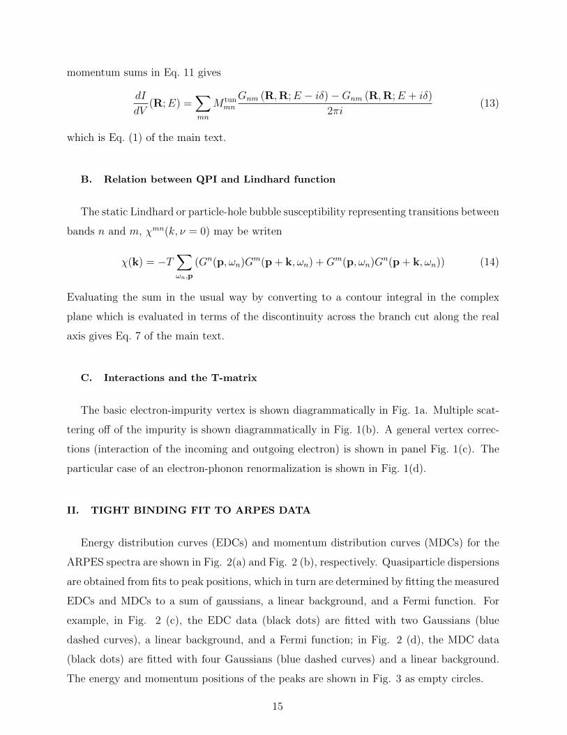
Energy distribution curves (EDCs) and momentum distribution curves (MDCs) for the

ARPES spectra are shown in Fig. 2(a) and Fig. 2 (b), respectively. Quasiparticle dispersions

are obtained from fits to peak positions, which in turn are determined by fitting the measured

EDCs and MDCs to a sum of gaussians, a linear background, and a Fermi function. For

example, in Fig. 2 (c), the EDC data (black dots) are fitted with two Gaussians (blue

dashed curves), a linear background, and a Fermi function; in Fig. 2 (d), the MDC data

(black dots) are fitted with four Gaussians (blue dashed curves) and a linear background.

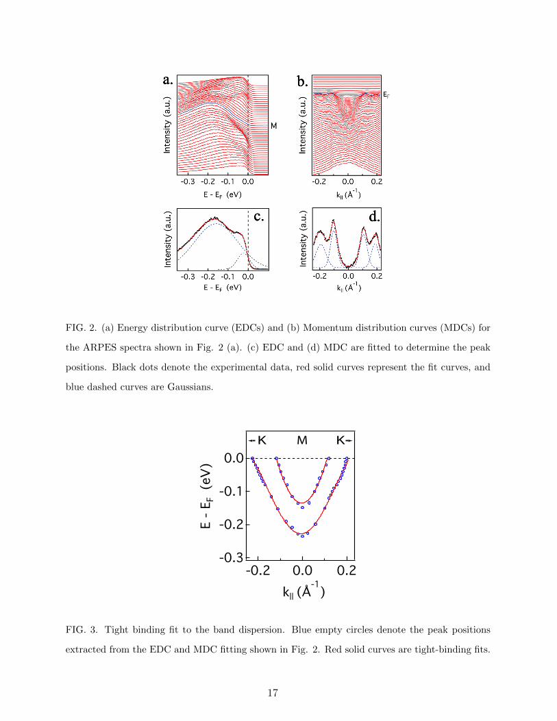
The energy and momentum positions of the peaks are shown in Fig. 3 as empty circles.

15

X X X X

X

(a) (b)

(c)

X

k

(d)

FIG. 1. Diagrammatic representation of electron impurity scattering. (a) single scattering event;

(b) example of multiple scattering from an impurity; sum of all such diagrams yield the bare

T-matrix; (c) single scattering event renormalized by general electron-electron interaction vertex

(d) single scattering event renormalized by phonon. Dashed line with X: bare electron-impurity

vertex; solid line with arrow: electron propagator as determined from ARPES (i.e. renormalized

by self energy); shaded box: general vertex correction; heavy double line: phonon propagator with

phonon momentum k indicated.

We fit these two bands to a previously-proposed [23] five-nearest-neighbor tight-binding

model to extract the band dispersions (red solid curves). The bands of the tight-binding

model are given by the following expression:

Ei(kx, ky) = t0,i + t1,i(2 cos(ηx) cos(ηy) + cos(2ηx))

+ t2,i(2 cos(3ηx) cos(ηy) + cos(2ηy))

+ t3,i(2 cos(2ηx) cos(2ηy) + cos(4ηx))

+ t4,i(cos(ηx) cos(3ηy) + cos(5ηx) cos(ηy)

+ cos(4ηx) cos(2ηy)) (15)

16

FIG. 2. (a) Energy distribution curve (EDCs) and (b) Momentum distribution curves (MDCs) for

the ARPES spectra shown in Fig. 2 (a). (c) EDC and (d) MDC are fitted to determine the peak

positions. Black dots denote the experimental data, red solid curves represent the fit curves, and

blue dashed curves are Gaussians.

M KK

FIG. 3. Tight binding fit to the band dispersion. Blue empty circles denote the peak positions

extracted from the EDC and MDC fitting shown in Fig. 2. Red solid curves are tight-binding fits.

17

with

ηx =1

2kxa ηy =

√3

2kya (16)

These expressions model the quasi two-dimensional Nb-derived bands that are observed

in ARPES experiments. A Se-derived band with strong kz dispersion is also found in DFT

calculations [18] but is typically not seen in ARPES [29]. The strong kz disperson of this

band also means that it will contribute less to the QPI. We do not consider it here. The

parameters of the model are given in Table I.

Parameter (meV) t0 t1 t2 t3 t4

Band 1 14.2 82.8 255.4 42.9 20.5

Band 2 265 21.0 407.2 8.8 -1.0

TABLE I. Tight binding parameters from ARPES. Note that in these conventions the Fermi energy

is set to 0.

From the tight binding parameters we calculate the components of B via the computa-

tionally efficient expression [18]:

Bnm(k, E) =

ˆ 0

−∞dα

ˆ ∞0

dβ

α− βFnm(α, β,k) (17)

Fnm(α, β,k) =

ˆdk′

(2π)2[δ(En(k′)− α)δ(Em(k′ + k)− β)] (18)

III. PARTIAL SUSCEPTIBILITY CALCULATED FROM STS

Proceeding from Eq. 5 of the main text we observe that if the T matrix has negligible

energy dependence and couples all bands equally then the integral of the measured QPI

signal over a range from −E0 (chosen such that E0 >> kT ) to the Fermi level is, up to a

constant, just an approximation χ0 to the sum of all components of the static susceptibility

χ:

ˆ 0

−E0

dEf(E)

∣∣∣∣δdI(k, E)

dV

∣∣∣∣ ∝ T (k)∑nm

ˆ 0

−E0

dEf(E)Bnm(k, E) = T (k)χ0(k) ≈ T (k)χ(k)

(19)

18

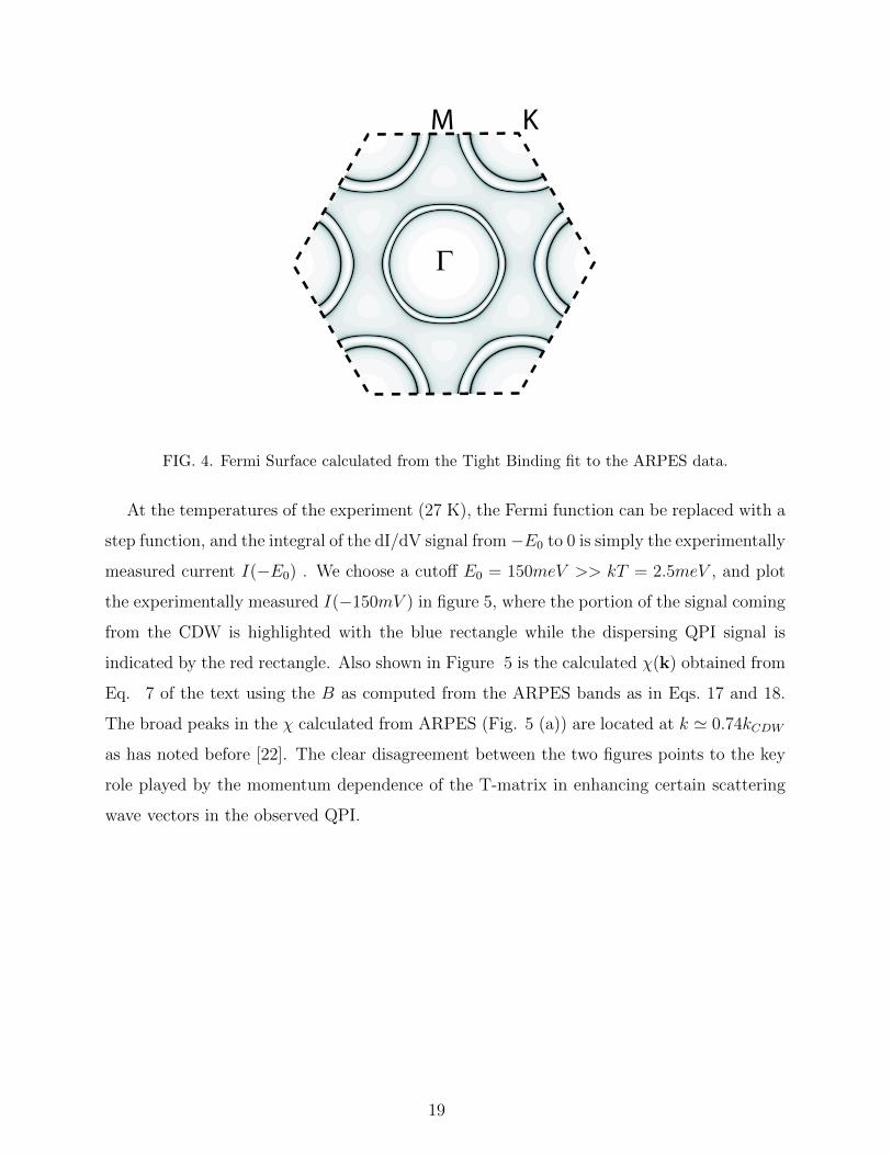
Γ

M K

FIG. 4. Fermi Surface calculated from the Tight Binding fit to the ARPES data.

At the temperatures of the experiment (27 K), the Fermi function can be replaced with a

step function, and the integral of the dI/dV signal from−E0 to 0 is simply the experimentally

measured current I(−E0) . We choose a cutoff E0 = 150meV >> kT = 2.5meV , and plot

the experimentally measured I(−150mV ) in figure 5, where the portion of the signal coming

from the CDW is highlighted with the blue rectangle while the dispersing QPI signal is

indicated by the red rectangle. Also shown in Figure 5 is the calculated χ(k) obtained from

Eq. 7 of the text using the B as computed from the ARPES bands as in Eqs. 17 and 18.

The broad peaks in the χ calculated from ARPES (Fig. 5 (a)) are located at k ' 0.74kCDW

as has noted before [22]. The clear disagreement between the two figures points to the key

role played by the momentum dependence of the T-matrix in enhancing certain scattering

wave vectors in the observed QPI.

19

Low

Higha b

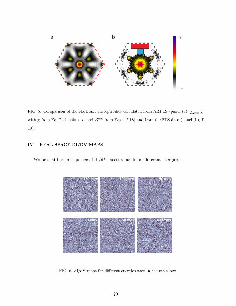
FIG. 5. Comparison of the electronic susceptibility calculated from ARPES (panel (a),∑

mn χmn

with χ from Eq 7 of main text and Bmn from Eqs. 17,18) and from the STS data (panel (b), Eq.

19).

IV. REAL SPACE DI/DV MAPS

We present here a sequence of dI/dV measurements for different energies.

150 meV 100 meV 50 meV

0 meV -50 meV -100 meV

FIG. 6. dI/dV maps for different energies used in the main text

20

V. COMPARISON BETWEEN FT-STS AND ARPES B

In Figure 7 we present an expanded view ot the comparison between the Fourier transform

of the measured STS data and the B calculated from ARPES at energies ranging from well

below the Fermi level to well above. We zoom in a particular region of k-space that shows

dispersing features. The left half of each subfigure is the FT-STS data while the right half

is the calculated B. The dispersing QPI feature is located along the Γ −M direction at

wavevectors larger than kCDW . Zooming in to the region of k-space where QPI is observed,

we see from Figure 7 that the FT-STS signal is located near the edge of the Brillouin zone

at energies well below EF , and disperses steadily inwards at higher energies. Within this

restricted region of k-space, the dispersion of the FT-STS data matches very well with the

B calculated from ARPES at all energies.

-50meV -100meV -70meV

-20meV

20meV 100meV

0meV

150meV

FIG. 7. Comparison between FT-STS and B calculated from ARPES at energies indicated. Shown

for each energy is a slice of k-space from the Brillouin zone boundary near the M point, inwards

to a wave vector somewhat larger than the CDW wave vector The left half of each subfigure is

the FT-STS data while the right half is the calculated B. Within the restricted region of k-space

shown, the dispersion of the FT-STS data matches very well with the B calculated from ARPES

at all energies.

21