QUBLE: towards blending interactive visual subgraph search ... · ... towards blending interactive...

The VLDB Journal (2014) 23:401–426DOI 10.1007/s00778-013-0322-1

REGULAR PAPER

QUBLE: towards blending interactive visual subgraph searchqueries on large networks

Ho Hoang Hung · Sourav S Bhowmick ·Ba Quan Truong · Byron Choi · Shuigeng Zhou

Received: 2 September 2012 / Revised: 21 February 2013 / Accepted: 4 June 2013 / Published online: 3 August 2013© Springer-Verlag Berlin Heidelberg 2013

Abstract In a previous paper, we laid out the vision ofa novel graph query processing paradigm where instead ofprocessing a visual query graph after its construction, it inter-leaves visual query formulation and processing by exploit-ing the latency offered by the gui to filter irrelevant matchesand prefetch partial query results [8]. Our recent attemptsat implementing this vision [8,9] show significant improve-ment in system response time (srt) for subgraph queries.However, these efforts are designed specifically for graphdatabases containing a large collection of small or medium-sized graphs. In this paper, we propose a novel algorithmcalled quble (QUery Blender for Large nEtworks) to real-ize this visual subgraph querying paradigm on very large net-works (e.g., protein interaction networks, social networks).First, it decomposes a large network into a set of graphletsand supergraphlets using a minimum cut-based graph parti-tioning technique. Next, it mines approximate frequent and

Electronic supplementary material The online version of thisarticle (doi:10.1007/s00778-013-0322-1) contains supplementarymaterial, which is available to authorized users.

H. H. Hung · S. S Bhowmick (B) · B. Q. TruongSchool of Computer Engineering, Nanyang TechnologicalUniversity, Nanyang Avenue, Singaporee-mail: [email protected]

H. H. Hunge-mail: [email protected]

B. Q. Truonge-mail: [email protected]

B. ChoiHong Kong Baptist University, Kowloon Tong, Hong Konge-mail: [email protected]

S. ZhouFudan University, Shanghai, Chinae-mail: [email protected]

small infrequent fragments (sifs) from them and identifiestheir occurrences in these graphlets and supergraphlets. Then,the indexing framework of [9] is enhanced so that the minedfragments can be exploited to index graphlets for efficientblending of visual subgraph query formulation and queryprocessing. Extensive experiments on large networks demon-strate effectiveness of quble.

Keywords Visual graph querying · Query formulation ·Frequent fragments · Small infrequent fragments ·Action-aware indices · Action-aware query processing ·Blending · Large networks

1 Introduction

Graphs are of increasing importance in modeling complexstructures such as molecular interactions, chemical com-pounds, social relationships, and program dependence. Dueto the explosive growth of graph-structured data in recentyears, querying graph databases has emerged as an impor-tant research problem for real-world applications that arecentered on large graph data. At the core of many of theseapplications lies a common and important query primitivecalled subgraph search, where we want to retrieve one ormore subgraphs in a set of data graphs that exactly orapproximately match a user-specified query graph. Effortsto address this problem can be broadly classified into twostreams [4]. One stream focuses on processing subgraphqueries on a large number of small or medium-sized graphs(e.g., [2,8,9,11,15,16]) such as chemical compounds. Theother stream aims to handle query processing on a small num-ber of large graphs (e.g., protein interaction networks, socialnetworks) [12,13,18–20]. In contrast to the former stream,there has been lesser research on the latter.

123

http://dx.doi.org/10.1007/s00778-013-0322-1

402 H. H. Hung et al.

Fig. 1 Visual interface for formulating graph queries

Concurrent to the aforementioned efforts toward effi-cient subgraph querying, a number of declarative graphquery languages (e.g., sparql, Graphql [5]) have alsobeen proposed that can be used to formulate these queries.Unfortunately, formulating a graph query using these lan-guages often demands considerable cognitive effort from auser and requires “programming” skill that is at least compa-rable to sql. Consequently, in many real-life domains (e.g.,life sciences), it is unrealistic to assume that users are profi-cient in expressing such queries textually.

1.1 A new visual querying paradigm

A popular way to alleviate the graph query formulation chal-lenge is to build a user-friendly graphical interface on top of agraph query processing technique. Figure 1 depicts an exam-ple of such a visual interface. A user begins formulating aquery by choosing a database as the query target and creatinga new query canvas using Panel 1. The left panel (Panel 2)displays unique labels of nodes that appear in the dataset. Inthe query formulation process, the user chooses labels fromPanel 2 for creating nodes in the query graph. Then, she dragsa node that is part of the query from Panel 2 and drops it inPanel 3. Next, she adds another node in the same way andcreates an edge between the added nodes by left and rightclicking on them. Additional nodes and edges are added tothe query graph by repeating these steps.1 Finally, the usercan execute the query by clicking on the Run icon in Panel 1.

In [1,8], we laid out the vision of a novel visual graphquery processing paradigm where we blend the two tradi-tionally orthogonal steps, namely visual query formulationand query processing, bringing in two key benefits. First, itensures that the query processor does not remain idle dur-ing query formulation. Second, it significantly improves the

1 In this paper, we assume an “edge-at-a-time” visual query formulationinterface. A more advanced and domain-dependent gui may supportdrag and drop of canned patterns or subgraphs (e.g., benzene ring) forcomposing visual queries. Such visual query composition interface isbeyond the scope of this work.

system response time (srt).2 In traditional graph processingparadigm, the srt is identical to the time taken to evaluatethe entire query as the query processor remains idle duringquery formulation. In contrast, in this new paradigm, the srt

is the time taken to process a part of the query that is yet tobe evaluated (if any). Note that from an end user’s perspec-tive, the srt is crucial as it is the time the user has to waitbefore she can view the results. More recently, we proposeda visual subgraph querying algorithm called prague [9] thatimplements this vision. Let us illustrate it with an example.

Consider a graph database containing a set of small ormedium-sized graphs (e.g., chemical compounds). prague

first mines and extracts frequent and infrequent graph frag-ments from this database using an existing frequent graphmining algorithm [14]. These fragments are then used toconstruct the action-aware frequent (a2

f) and action-awareinfrequent indexes (a2

i). Suppose a user constructs a querygraph using the gui in Fig. 1. prague utilizes the latencyoffered by the gui actions to retrieve partial candidate datagraphs. For each new edge constructed by the user, it usesthe action-aware indexes to generate an on-the-fly dynamicindex called spindle-shaped graph (spig), which succinctlyrecords various information related to the set of supergraphsof the new edge in the visual query fragment. Using theseindexes, it retrieves identifiers of data graphs containing thequery fragment q (denoted by Rq ). If q is a frequent fragmentor a discriminative infrequent fragment (dif), then the iden-tifiers are retrieved by probing the a

2f-index or a

2i-index,

respectively. Note that a dif is an infrequent fragment whosesize is either one or all its subgraphs are frequent. If q is nei-ther a dif nor a frequent fragment, then prague exploits thespigs to generate the candidate set. If Rq becomes empty (thequery fragment does not have any matches), then it exploitsthe spig set again to retrieve approximate matches3 to q. Thiscontinues until the user clicks on the Run icon, when finalquery results are computed. Specifically, if the final queryis a frequent subgraph or a dif, then the results are directlycomputed without subgraph isomorphism test. If it is a non-dif infrequent query, then the exact results are computed byfiltering false candidates using subgraph isomorphism test.Otherwise, if the final query has no exact match, then itsapproximate matches are generated using spigs and, if nec-essary, by extending VF2 [3] to handle mccs-based similarityverification. Note that the above paradigm can be efficientlyrealized even when a user modifies a query at any time duringquery formulation [9].

2 Duration between the time a user presses the Run icon to the timewhen the user gets the query results [8].3

prague adopts the maximum connected common subgraphs (mccs)for computing similarity between a pair of graphs.

123

QUBLE: towards blending interactive 403

1.2 Motivation

prague is designed specifically for graph databases con-taining a large collection of small or medium-sized graphs.Consequently, its indexing schemes and query processingstrategy are designed to efficiently support query matchingon such data graph collection. Unfortunately, these schemescannot be easily adopted to support subgraph queries on largenetworks containing thousands of nodes and edges. This isprimarily because the frequent and infrequent fragments-based indexing strategy adopted in prague is impracticalfor this case. Specifically, a graph fragment is consideredfrequent if the number of data graphs containing it is noless than a certain support threshold α. Now suppose wehave a single large graph with 100,000 nodes and 200,000edges. Then, prague can only identify frequent fragmentsif α is set to either zero or one. If α is set to one, then allsubgraphs of the data graph can be considered as frequent.However, this is prohibitively expensive to index as thereare more than one billion subgraphs. Even if an index couldbe constructed, a non-dif infrequent query would requirea subgraph isomorphism test against a data graph having100,000 nodes, which is prohibitively expensive. In contrast,it is not explosive in the context of small or medium-sizedgraph collection as we only need to keep track of identi-fiers of data graphs that contain a frequent fragment or dif

and the subgraph isomorphism test is against small-sizedgraphs.

At a first glance, it may seem that the aforementioned bot-tleneck is due to the way frequent and infrequent fragmentsare defined in the prague framework. However, in general,generating frequent subgraphs for indexing is itself a bottle-neck for the case of large networks [13]. This is because thetime complexity of subgraph isomorphism, the core routineof any frequent subgraph mining algorithms, grows expo-nentially with the graph size. Furthermore, these subgraphsmay suffer from low selectivity issue [13], reducing the effec-tiveness of the indexes. Small-sized frequent fragments typ-ically have low selectivity as they may occur many times.As a result, they may generate a large number of candidatesagainst small-sized query fragments.

The indexing scheme of prague is not the only stum-bling block for realizing the new visual querying paradigm onlarge networks. Visualizing query results is also a challeng-ing issue. In prague, it is straightforward to visually displayeach data graph satisfying a query graph as the number ofnodes in each data graph is small. However, visualizing themin a large network becomes cognitively and computationallychallenging. Even if a data graph contains few thousands ofnodes and edges, it imposes significant cognitive burden onan end user if it is shown in its entirety. Particularly, the entirenetwork looks like a giant hairball and subgraphs that matcha query are lost in the visual maze. In this paper, we propose

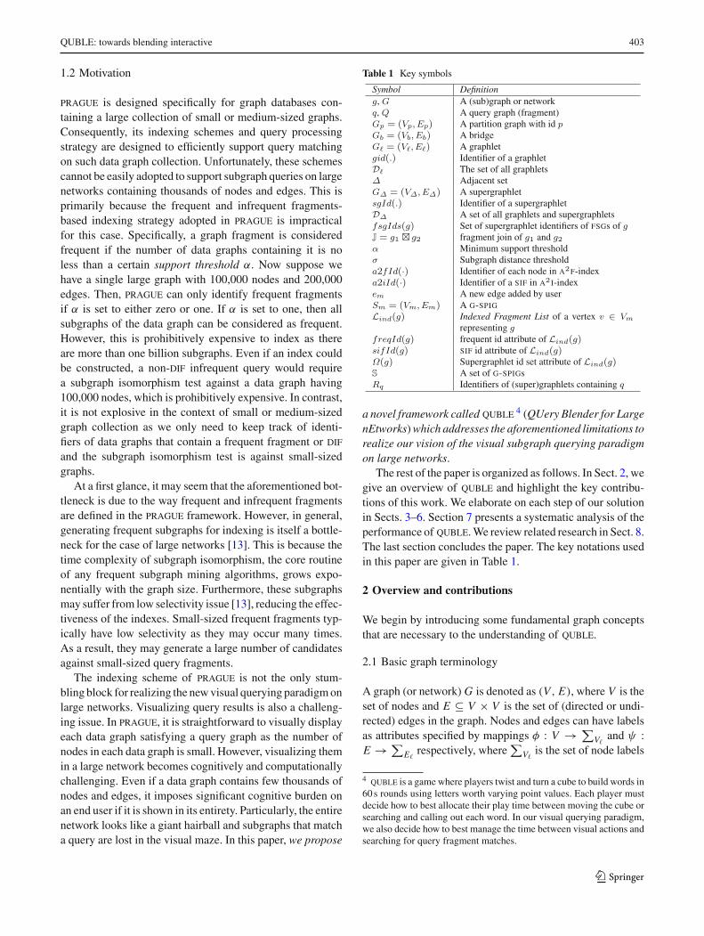
Table 1 Key symbols

a novel framework called quble4 (QUery Blender for Large

nEtworks) which addresses the aforementioned limitations torealize our vision of the visual subgraph querying paradigmon large networks.

The rest of the paper is organized as follows. In Sect. 2, wegive an overview of quble and highlight the key contribu-tions of this work. We elaborate on each step of our solutionin Sects. 3–6. Section 7 presents a systematic analysis of theperformance of quble. We review related research in Sect. 8.The last section concludes the paper. The key notations usedin this paper are given in Table 1.

2 Overview and contributions

We begin by introducing some fundamental graph conceptsthat are necessary to the understanding of quble.

2.1 Basic graph terminology

A graph (or network) G is denoted as (V, E), where V is theset of nodes and E ⊆ V × V is the set of (directed or undi-rected) edges in the graph. Nodes and edges can have labelsas attributes specified by mappings φ : V → ∑

V� and ψ :E →∑

E� respectively, where∑

V� is the set of node labels

4quble is a game where players twist and turn a cube to build words in

60 s rounds using letters worth varying point values. Each player mustdecide how to best allocate their play time between moving the cube orsearching and calling out each word. In our visual querying paradigm,we also decide how to best manage the time between visual actions andsearching for query fragment matches.

123


and∑

E� is the set of edge labels. Each node in V is assigneda unique identifier. The size of G is defined as |G| = |E |. Forease of presentation, we present our method using undirectedgraphs with labeled nodes. It is straightforward to extendour method to process edge-labeled and/or directed graphs.Besides, we assume that a query graph has at least one edgeand all nodes in it are connected (no dangling edges or nodes).

A graph G1 = (V1, E1) is a subgraph of another graphG2 = (V2, E2) (or G2 is a supergraph of G1) if there exists asubgraph isomorphism from G1 to G2, denoted by G1 ⊆ G2

(or G2 ⊇ G1). We may also simply say that G2 contains G1

or G2 is an exact match of G1. The graph G1 is called a propersubgraph of G2, denoted as G1 ⊂ G2, if G1 ⊆ G2 andG1 � G2. Given two connected graphs G1 and G2, if G1 isa subgraph of G2 and |G2| = |G1|+1, then we refer to G1 as aparent graph of G2. Lastly, given a graph G, let G1 and G2 besubgraphs of G. Let G1 is isomorphic to G ′1 = (V ′1, E ′1) ⊆ Gand G2 is isomorphic to G ′2 = (V ′2, E ′2) ⊆ G. Then, G1 andG2 is said to overlap in G if V ′1∩V ′2 �= ∅ and E ′1∩ E ′2 �= ∅.

2.2 Subgraph similarity search problem

Existing works on subgraph query processing over largenetworks typically focus on two types of queries, namelysubgraph containment [12,13,18] and subgraph similar-ity [12,19,20]. The former focuses on indexing a large net-work G, so that we can efficiently find all or a subset ofexact matches of a given query graph in G, whereas the lat-ter seeks for approximate matches to the query. The word“approximate” refers to matches to the query that allow miss-ing edges or nodes. Note that as large graphs typically haveintricate structures and can be noisy (e.g., protein interac-tion networks), support for approximate matches is crucialin real-world applications [19]. Hence, in this work, we aimto support both subgraph containment and subgraph similar-ity queries on large networks.

The core component of the evaluation mechanism ofsubgraph similarity queries is the notion of graph similar-ity. Recently, two types of distance measures are exploitedto measure similarity between two graphs (not necessarilylarge), namely graph edit distance [17] and maximum con-nected common subgraph [11]. In the former approach, thesimilarity of two graphs is defined by the least edit opera-tions (insertion, deletion, and relabeling) used to transformone graph into another. Each of these operations relaxes thequery graph by removing or relabeling one edge. The latterapproach detects maximum connected common subgraphs(mccs). Given two graphs Q and G, a connected commonsubgraph (ccs) of Q and G is a connected subgraph of Qthat is subgraph isomorphic to G. The maximum connectedcommon subgraph of Q and G is the largest ccs. In spite ofthe applicability of edit distance for any type of graphs and itssuperior quality of results over mccs for several cases [17],

in this paper we adopt a variant of the latter as it is moreamenable to a visual querying system as justified in [9].

Definition 1 (Subgraph distance) Given two graphs G andQ, let CQ ⊆ G be a connected common subgraph (ccs) of Qand G. Then, the subgraph distance, denoted as distC (Q,G),is defined as follows: distC (Q,G) = |Q| − |CQ |.

The subgraph distance measures the number of edges thatare allowed to be missed in Q in order to match G. There canbe many subgraphs of G that are ccs of Q and G. Hence,subgraphs with smaller dist are more similar to Q. Notethat if distC (G1,G2) = 0, then G1 and G2 are subgraphisomorphic to each other.

Definition 2 (Subgraph similarity search) Given a querygraph Q, a large network G, and a subgraph distance thresh-old σ , the goal of the subgraph similarity search problem isto retrieve all connected common subgraphs Ci of Q and Gs.t distCi (Q,G) ≤ σ .

Observe that we use ccs instead of mccs for similaritysearch. This is because we aim to find all similar matcheswhose size may be smaller than that of an mccs as long as it iswithin σ . We believe that this feature is especially importantin large networks having intricate structures or noise.

Remark A keen reader may note the difference between theabove definition of subgraph distance and the edge edit dis-tance used in sapper [19] and TreeSpan [20] for similaritysearch. Specifically, these approaches propose to generate allapproximate occurrences of a query graph q in G by enumer-ating all connected subgraphs g in G such that g is at most θedges away to be isomorphic to q. That is, these approachesallow missing edges but not missing nodes.5 Consequently,the similar matches are “restrictive” as they must containsame number of nodes as the query graph. In contrast, quble

allows both missing edges and nodes, enabling it to retrievesimilar subgraphs that do not necessarily have the same num-ber of nodes as the query graph.

2.3 Overview of QUBLE

Can we somehow leverage the action-aware indexes andspigs because they have efficiently supported our visualquery paradigm on a large collection of small or medium-sized graphs? Unfortunately, this is challenging as it requiresus to determine frequent fragments in a large network whichis prohibitively expensive operation and a long-standingproblem [13]. Hence, techniques described in [8,9] cannotbe directly adopted to this new scenario. Furthermore, it is

5 Extension of TreeSpan is claimed to support vertex mismatch. How-ever, the details are not discussed in [20].

123


Algorithm 1: INDEXGENERATION

Input: A large network G, support threshold α, partitionthreshold p.

Output: Action-aware indexesG ← metis(G, p);1D� ← GraphSetConst(G) /* Algorithm 3 */;2F ← gSpan(D�, α) ;3Group frequent fragments F by size;4(F, I)← TwoEdgeFragment(F, I,D�) /* Algorithm 6 */;5F ← CompleteFreqFrag(F,DΔ) /* Algorithm 7 */;6I ← CompleteSIF(I,D�) /* Algorithm 8 */;7Build action-aware indexes using (F, I);8

also highly space consuming to index location of all possi-ble occurrences of a feature in a large intricate network as itmay appear numerous times. We address these challenges inquble by taking the following steps. First, we decompose alarge network into pieces of small data graphs while ensur-ing that no structural information is lost during this process.Consequently, the decomposed graph set can be viewed asa collection of small or medium-sized data graphs. Second,we discover approximate sets of frequent and infrequent frag-ments from this collection and identify their occurrences inthe data graphs. This associates each fragment with a listof data graph identifiers instead of a full location list in theoriginal network, which is very storage efficient. Third, weredefine and build action-aware indexes and spigs over thesedecomposed graphs to support subgraph search. We nowbriefly describe these steps.

Action-aware index construction. Algorithm 1 outlines theprocedure for generating action-aware indexes in quble. Wedecompose a large network to pieces of small data graphscalled graphlets by exploiting metis [10], a fast and widelyused minimum cut-based graph partitioning algorithm (Lines1–2). A graphlet is either a partition graph or a bridge. Infor-mally, partition graphs are partitions generated by the graphpartitioning algorithm on the original network. On the otherhand, bridges are graphs that are constructed from cut edgesthat link certain pairs of partition graphs for instance con-sider the network in Fig. 2. The subgraphs with ids G1 to G4

(subgraphs encompassed by thick lines) are partition graphsgenerated by the graph partitioning technique. The bridgeslink certain pairs of these partition graphs (shown by pat-terned nodes encompassed by dotted lines) and are denotedby G5 to G7 (e.g., G5 linking G1 and G2). These seven datagraphs are collectively referred to as graphlets.

Next, we mine these graphlets to extract frequent and smallinfrequent fragments (sif) and their occurrences and use themto create graphlet-based indices and graphlet-based spigs(g- spig), which are variants of the original action-awareindices and spigs used in prague [9], respectively. At firstglance, it may seem that we can use an existing frequentsubgraph mining algorithm (e.g., gSpan [6]) to identify allfrequent fragments from the graphlet set (Line 3). Unfortu-nately, such approach can only identify all size-one frequent

Fig. 2 A network. The numbers within the nodes are labels and notnode ids

23 0 4

7 2 5 19 7 2

19 7 2 5

(a) g1 (b) g2

(c) g3 (d) g4

Fig. 3 Query fragments

fragments as an edge can only belong to exactly one graphlet.However, due to cut-based partitioning of the network, it failsto find all frequent fragments (having size two or more) aswell as their occurrences as such a fragment may be containedin a subgraph involving multiple adjacent graphlets insteadof a single graphlet for instance consider the graphlets inFig. 2 and the fragment g1 in Fig. 3a. Observe that althoughthere are three occurrences of g1 in the original network,only one of them occurs in the graphlet G2. The remain-ing two are subgraphs of adjacent graphlets (G3, G6) and(G4, G7). Hence, if the support threshold is set to 2, then g1

will be identified as an infrequent fragment instead of a fre-quent one. Furthermore, only the occurrence of g1 in G2 willbe identified by the aforementioned approach. Consequently,we need to devise strategies to address this challenge.

The aforementioned challenge raises two important issues.First, do we need to identify all frequent fragments or a par-tial set is sufficient? How do we identify them? Second, irre-spective of whether a fragment is frequent or infrequent, weneed to devise a technique to obtain complete sets of occur-rences of these fragments to facilitate subgraph search. Howcan we identify and index them efficiently?

Fortunately, as we shall see in Sect. 7, it is not neces-sary to identify all frequent fragments to support efficientvisual subgraph query processing in our paradigm. A partial

123


Algorithm 2: quble

Input: gui Action, query q, candidate set Rq , subgraph distancethreshold σ , supergraphlet set DΔ, g- spig set S.

Output: Query results Resultsif Action is New then1

q ← q + em ;2Sm ← GSpigConstruct(q, Q, em , S) /*Algorithm 9*/;3Rq ← ExactSubCandidates(Sm .vtarget )4/*Algorithm 10*/;(R f ree, Rver )← SimilarSubCandidates(q, σ, S)5/*Algorithm 11*/;

else if Action is Run then6Results ← ExactVerification(q, Rq , S,DΔ)7/*Algorithm 12*/;Results ←8SimilarResultsGen(q, R f ree, Rver , Results, σ )

/*Algorithm 13*/;

set of frequent fragments is sufficient for our goal. Conse-quently, frequent fragments that are not identified as frequentby quble are categorized as infrequent (e.g., g1 is classifiedas infrequent in the above example). Importantly, as we shallsee later, such “miscategorization” does not adversely impactthe accuracy of quble. The second issue, however, needs tobe addressed carefully to support efficient subgraph queryprocessing. Regardless of whether a fragment is frequent orsif, all occurrences of the fragment must be identified andindexed (e.g., all three occurrences of g1 must be identi-fied). We exploit the notion of supergraphlets to identify anapproximate set of frequent fragments as well as finding alloccurrences of frequent fragments and sifs.

Notice that some nodes in Fig. 2 belong to multiplegraphlets. Graphlets that share some nodes but not edgesare referred to as adjacent. Hence, we can combine adja-cent graphlets together to create a new graph called super-graphlet. For example, in Fig. 2, G3 and G6 are adja-cent graphlets which are combined together to form thesupergraphlet G8 (subgraph shaded in yellow). Observe thatg1 ⊆ G8. Obviously, constructing all possible supergraphletsis prohibitively expensive. Hence, they are selectively con-structed to identify all occurrences of frequent fragments andsifs. Specifically, the procedures in Lines 4–7 are invoked toachieve this (detailed in Sect. 4).Blending of visual query. When a user constructs a visualquery graph step-by-step, these graphlet-based indices areleveraged to generate candidate graphlets and supergraphlets.After every visual action taken by a user, the current queryfragment is evaluated by exploiting the latency offered by thegui. Algorithm 2 is invoked whenever a user adds an edgeduring visual query formulation.6 Let q be the visual querybeing formulated by a user. There are two visual actions onthe gui being monitored, namely New for addition of a new

6 A video of quble is available at http://youtu.be/4k4XBxxdD_4. It isalso demonstrated in SIGMOD 2013 [7].

Fig. 4 Visualizing result matches in quble. Panel 2 shows the list ofsupergraphlet identifiers containing matched results

edge, and Run for executing q.7 When a user adds a newedge em to q, the algorithm first constructs the graphlet-based spindle-shaped graph (g- spig) Sm for em (Line 3).It then computes the identifiers of candidate graphlets andsupergraphlets that contain q using Sm and the action-aware indexes by invoking the ExactSubCandidates proce-dure (Line 4). Next, for a given σ , identifiers of candidatesthat match approximately with q is retrieved by exploitingthe g- spig set S. This is encapsulated in the procedure Simi-larSubCandidates (Line 5). The above steps are repeated foreach new edge to incrementally update candidate identifiersuntil the Run icon is clicked (Line 6). Subgraphs that exactlymatch the query are verified (if necessary) from the candidategraphs and stored in Results (Line 7). Next, candidates thatmatch the query approximately are added to Results (Line8). We shall elaborate on these procedures in Sects. 5 and 6.

In quble, query results generated by the above processare visually displayed to a user. Recall from Sect. 1, visu-alizing subgraphs that match (or similar to) a query graphis challenging as depicting them on the entire networkprohibitively increases the cognitive burden on end users.Fortunately, the advantage of decomposing a network intographlets and supergraphlets is not only limited to storageefficiency achieved by compressing the location informationof a fragment (feature) g into a list of (super)graphlets iden-tifiers where g is a subgraph. We can also leverage themto visually show the results of a query on each graphletor supergraphlet that contains at least one instance of theresult. Specifically, results are viewed in a “supergraphlet-at-a-time” mode where one supergraphlet or graphlet con-taining result matches is displayed on the results screen oneat a time. Figure 4 depicts an example where a matched resultis highlighted with different color in a supergraphlet. Observethat such supergraphlet-driven view enables a user to clearlylocate a matched result and understand its relationship with

7 Note that we do not monitor action for modifying the query fragmenthere as the procedure is same as in prague [9].

123

http://youtu.be/4k4XBxxdD_4


neighboring nodes. Additionally, it allows a user to selec-tively initiate viewing all matches to a query graph at a par-ticular location of the network by interactively invoking an allmatches computation technique (discussed later) on a viewedsupergraphlet. Note that since the size of a (super)graphletis significantly smaller, the remaining matches to a querygraph in the viewed supergraphlet can be quickly computedas demonstrated in Sect. 7. Note that in [19,20], all matchesare directly computed for the entire network without humanintervention. Hence, our quble framework enables us to savecomputational cost by selectively computing all matches ina specific area of the network as demanded by an end user.

In Sect. 7, our experimental study demonstrates thatquble has excellent performance as the index construc-tion time and system response time (srt) grow gracefullywith increasing size of the network. Importantly, similar toour previous studies [8,9], our results show that the latencyoffered by the gui at every step during visual query for-mulation is sufficient to efficiently support subgraph queryprocessing over large networks (up to a million of nodes) inthis visual paradigm. In summary, the main contributions ofthis paper are as follows.

• To the best of our knowledge, this is the first effortto blend visual subgraph query formulation and queryprocessing on large networks.• We take the first step to demonstrate how the notion of

frequent and infrequent fragments can be exploited tofacilitate subgraph querying on large networks. Specifi-cally, we present algorithms to decompose a network intoa set of graphlets and supergraphlets and mine approx-imate frequent fragment set and sifs as well as theiroccurrences from them. These fragments are then used toconstruct action-aware indexes to support the new visualsubgraph querying paradigm.• We present a dynamic on-the-fly index structure called

graphlet-based spindle-shaped graph (g- spig), which isa variant of the spig structure used in [9], to facilitateefficient pruning and retrieval of partial results duringvisual query formulation. Specifically, we describe howsubgraph containment and similarity search can be per-formed by efficiently exploiting g- spigs and the latencyoffered by a visual querying environment.• By applying quble to large datasets, we show its effec-

tiveness, significant improvement of the srt over state-of-the-art methods based on the traditional paradigm, andability to handle large networks for interactive subgraphquerying.

3 Decomposition of a large network

We now describe in detail how we decompose a large networkinto small pieces of graphlets and supergraphlets.

3.1 Graphlets and adjacent graphlets

As mentioned in the preceding section, we first partition alarge network into a set of partition graphs and bridges usinga cut-based graph partitioning algorithm (e.g., metis [10]).Note that the task of such graph partitioning algorithm is toassign a single partition number to each node of the inputnetwork based on the required number of nodes in one par-tition. Edges that connect nodes that have different partitionnumbers are “cut” away. The goal is to minimize edge-cutwhile trying to achieve the required number of nodes in apartition. After the partitioning, each node v is assigned apartition number pid(v). Note that we are assuming an envi-ronment in which partitioning occurs once, while subgraphquery processing can occur many times; therefore, in thesequel, we focus on the effect partitioning has on subgraphquerying, not on the cost of partitioning itself. Additionally,although quble exploits metis, it is not tightly coupled toany specific graph partitioning technique. This enhances gen-erality of quble as it can be easily realized on top of anysuperior cut-based graph partitioning technique (by replac-ing metis in Line 1 in Algorithm 1 with another partitioningtechnique).

Definition 3 (Partition graph) A partition graph G p =(Vp, E p), with id p, is a subgraph of G = (V, E) where∀vi ∈ V, vi ∈ Vp iff pid(vi ) = p.

For example, the subgraphs with ids G1 to G4 in Fig. 2 arepartition graphs generated by a cut-based graph partitioningtechnique.

Definition 4 (Bridge) Given two partition graphs G p1 andG p2 of G = (V, E)where p1 �= p2, a bridge of G p1 and G p2

is a graph Gb = (Vb, Eb) that satisfies the followings: (a)∀vi ∈ V, vi ∈ Vb iff pid(vi ) = p1 and ∃ an edge (vi , v j ) s.t.v j ∈ V and pid(v j ) = p2; (b) ∀e = (v1, v2) ∈ E, e ∈ Eb

iff pid(v1) = p1 and pid(v2) = p2.

Informally, a bridge is constructed from cut edge(s) thatlink certain pair of partition graphs. For example, G6 is abridge of partition graphs G2 and G3. In this paper, we referto a partition graph or bridge collectively as graphlet. Eachgraphlet (denoted by G�) is identified by a unique identifier,denoted by gid(G�) (or gid� for brevity). Clearly, based onthe above definitions, any edge in the original network canonly belong to exactly one graphlet. A node in a graphletG� is called a boundary node iff its degree in G� is less thanits degree in the original network G. Since each edge of Gbelongs to exactly one graphlet, boundary nodes belong tomore than one graphlet. Notice that all nodes of a bridge areboundary nodes. In the sequel, we denote the set of graphletsgenerated from G as D�.

Two graphlets G�1 = (V�1, E�1) and G�2 = (V�2 , E�2)

are adjacent iff V�1 ∩ V�2 �= ∅ and E�1 ∩ E�2 = ∅. That is,

123


adjacent graphlets share some common nodes in the originalnetwork but not edges. For example, in Fig. 2, G5 and G1

are adjacent graphlets. Notice that adjacent graphlets are dif-ferent from overlapping graphs where both nodes and edgesmust be shared. Clearly, two partition graphs (e.g., G1 andG2 in Fig. 2) cannot be adjacent because each node has asingle partition number and cannot belong to two differentpartition graphs at the same time. A set of graphlets is con-sidered as an adjacent set (denoted as Δ) iff each graphlet isadjacent to at least one other graphlet in the set. For example,Δ = {G3,G4,G6,G7} because G3 is adjacent to G6 and G7

while G4 is adjacent to G7.Construction of graphlets. We now briefly describe the pro-cedure to construct graphlets from the original network. Wefirst obtain the partition graphs using metis [10]. It takes asinput the original network and a partition threshold, whichspecifies the target number of nodes in each partition graphs.metis will then assign one partition number to each node inthe original network. Algorithm 3 outlines the procedure forgraphlets construction. To construct a partition graph, nodesof the same partition are grouped together. If there is an edgebetween any two of these nodes in the original network, itwill be added into the partition graph. To construct a bridge,for each pair of adjacent nodes in the original network, if theirpartition numbers are different, the two nodes and their edgewill be added to the corresponding bridge. Observe that G isscanned only once and the time complexity of constructingthe graphlet set is O(|V |dmax) where dmax is the maximumdegree of a node in G.

3.2 Supergraphlets

A supergraphlet is a graph generated by merging a set ofadjacent graphlets. Formally, let Δ = {G�1,G�2 , . . . ,G�n }be an adjacent set and n ≥ 2. Then, a supergraphlet GΔ =(VΔ, EΔ) ofΔ is a graph satisfying the followings: (a) ∀ v ∈VΔ, v ∈ V�i where 0 < i ≤ n and (b) ∀e ∈ EΔ, e ∈ E� j

where 0 < j ≤ n. For example, reconsider Fig. 2. Let Δ ={G3,G6}. Then, the supergraphlet ofΔ is G8. In the sequel,we denote the set of all graphlets and all supergraphlets thatcan be constructed from the original network G as DΔ.

Each supergraphlet GΔ is assigned a supergraphlet iden-tifier, denoted by sgI d(GΔ) (sgI d for brevity when the con-text is clear), which is generated based on the identifiers ofthe graphlets in Δ. A supergraphlet identifier is a concate-nation of the identifiers of all graphlets in the adjacent setof a supergraphlet in ascending order. Formally, sgI d(GΔ)

is gid(G�1) − gid(G�2) − · · · − gid(G�n ) where ∀G�i ∈Δ, gid(G�1) < gid(G�2) < · · · < gid(G�n ). For example,let gid(G3) = 3 and gid(G6) = 6 (Fig. 2). Then, the super-graphlet identifier of G8 is 3–6. We denote a gid(G�i ) con-tained in an sgI d(GΔ) as gid(G�i ) ∈ sgI d(GΔ). Observethat a gid can be considered as a special case of supergraphlet

Algorithm 3: GraphletSetConst

Input: Partitioned graph set GOutput: Graphlet set D�

foreach v ∈ G do1pid(v)← partition number of v;2Add v into partition graph G p in D� whose gI d = pid(v);3

foreach vi ∈ G do4pid(vi )← partition number of vi ;5foreach v j in the adjacent list of vi in G do6

pid(v j )← partition number of v j ;7if pid(vi )=pid(v j ) then8

Connect (vi , v j ) in G p whose gI d = pid(vi );9else10

Add vi , v j into corresponding bridge Gb in D�;11Connect (vi , v j ) in Gb;12

identifier containing only a single identifier. Hence, in thesequel, we shall use the supergraphlet identifier to denote agraphlet identifier as well.

We define two operations, union and intersection, onsupergraphlet identifiers. Given sgI d(GΔ1) and sgI d(GΔ2),the union of these two identifiers, denoted as sgI d(GΔ1 ∪GΔ2) (sgI dΔ1∪Δ2 for brevity), is a sgI d which contains alldistinct graphlet identifiers of sgI d(GΔ1) and sgI d(GΔ2).On the other hand, the intersection of sgI d(GΔ1) andsgI d(GΔ2), denoted as sgI d(GΔ1 ∩ GΔ2) (sgI dΔ1∩Δ2 forbrevity), is a new sgI d which consists of graphlet identifiersthat appear in both sgI d(GΔ1) and sgI d(GΔ2). For exam-ple, let sgI d(GΔ1) =3–7 and sgI d(GΔ2) =4–7. Then,sgI d(GΔ1 ∪ GΔ2) =3–4–7 and sgI d(GΔ1 ∩ GΔ2) = 7.

Definition 5 [Maximal cover graph (mcg)] Let GΔ be thesupergraphlet of the adjacent set Δ = {G�1,G�2 , . . . ,G�n }.A graph Q is called maximal cover graph (mcg) of GΔ

if Q is isomorphic to G ′ = (V ′, E ′) where G ′ ⊆ GΔ and∀G�i ∈ Δ, ∃e ∈ E ′ s.t e ∈ E�i . Q is said to have a covermatch in the original network G.

Example 1 Consider the graph fragment g1 in Fig. 3a. Thereis a subgraph isomorphism from g1 to the supergraphlet GΔ1

where Δ1 = {G3,G6}. There are two edges in g1 where theedge (v7, v2) belongs to the bridge G6 and the edge (v2, v5)

belongs to the partition graph G3. Hence, g1 is an mcg ofGΔ1 . Similarly, g1 is also contained in the supergraphletGΔ2 where Δ2 = {G4,G7}. Specifically, edges (v7, v2)

and (v2, v5) belong to G7 and G4, respectively. Hence, g1

is also an mcg of GΔ2 . We can also say that g1 has two covermatches in the network. On the contrary, g1 is not an mcg ofGΔ3 where Δ3 = {G4,G6,G7}.Construction of supergraphlets. We now present the proce-dure to construct a supergraphlet GΔ from its adjacent setΔ.Note that supergraphlets are constructed only during indexconstruction and when we need to perform a subgraph ver-ification (i.e., to verify if a supergraphlet actually contains

123


Algorithm 4: SupGraphletConst

Input: Adjacent set Δ, graphlet set D�

Output: Supergraphlet GΔ

Initialize map A for representing adjacent nodes of each node ;1foreach gidi of G�i in Δ do2

Load graphlet G�i with graphlet id gidi from D�;3foreach v ∈ G�i do4

vid ← vertex id of vi ;5Add adjacency list of v in G�i into A.vid;6

foreach vid in the keyset of A do7Construct node v with id vid;8Add v into GΔ;9

foreach vid in the keyset of A do10foreach vid ′ in A.vid do11

if vid < vid ′ then12Connect (vid, vid ′) in GΔ;13

Set GΔ’s sgI d;14

a (sub)graph). Algorithm 4 outlines the steps. It makes useof a map data structure, denoted by A, which maps a nodev’s identifier (vid) to the adjacent nodes (vids) of v. It firstloads all graphlets associated with the identifiers in the adja-cent set Δ. For each node v in each graphlet, the algorithmadds v’s adjacency list into the list mapped by v’s identifierin A (Lines 2–6). Notice that v’s id is unique in the originalnetwork and not just unique within a graphlet. Also, somenode identifiers may exist in more than one graphlet as onenode can belong to more than one graphlet.

After creating A, for each value vid in the keyset of A,a node with id equal to vid is constructed and added to GΔ

(Lines 7–9). After the addition of all nodes, we process theid lists in A. For each node id vid ′ in each list, if it is greaterthan the associated key vid, then an edge connecting nodeswith identifiers vid and vid ′ is constructed in GΔ (Lines 10–13). Notice that since the graph is undirected, a node iden-tifier comparison is required to avoid duplicate constructionof edges. Finally, the supergraphlet identifier of GΔ is setaccordingly (Line 14). The time complexity of constructinga supergraphlet is O(Ndmax) where dmax is the maximumdegree of a node in the adjacency set.

Example 2 Consider the adjacent set Δ = {G1,G5}. Forgid(G1) = 1, for each node having vids from 1 to 24 (in G1),its adjacency list in G1 is added into the node id list associatedwith the key vid in A for instance v1 is adjacent to v4 andv5 in G1. Hence, 4 and 5 are added into the adjacency listassociated with key 1 in A. Similarly, for gid(G5) = 5, v24

is adjacent to v25 in G5. Hence, 25 and 24 are added into thelists associated with keys 24 and 25, respectively. After Line8, A has a keyset of 25 values ranging from 1 to 25. Hence,25 nodes with these ids are added to the supergraphlet. Thecorresponding 25 node id lists associated with A are thenused to create the edges. For example, for the list with key 1,since 4 > 1 and 5 > 1, edges (v1, v4) and (v1, v5) are added

into the supergraphlet. Finally, the supergraphlet identifier isset to 1–5.

4 Indexing frequent and infrequent fragments

In this section, we begin by defining the notion of frequentand infrequent fragments in the context of graphlets andsupergraphlets. Next, we introduce the notion of fragmentjoin, which we shall leverage for frequent and infrequentfragments generation. Then, we present algorithms for gen-erating frequent and infrequent fragments from the decom-posed network. Lastly, we briefly present how the action-aware indices of prague [8,9] are adopted to index thesefragments.

4.1 Frequent and infrequent fragments

Let g be a subgraph of G� or GΔ in DΔ and has at leastone edge. Then, g is a fragment in DΔ. Given a fragmentg ⊆ Gi and Gi ∈ DΔ, Gi is called a fragment support graph(fsg) of g. Recall that each graphlet or supergraphlet can beidentified by a supergraphlet identifier. Hence, we denote aset of supergraphlet identifiers of fsgs of g as f sgI d(g).Then, the support of g, denoted as sup(g), is the number ofgraphlets that are fsgs of g. Recall from Sect. 2.3, we identifyan initial set of frequent fragments by mining the graphletsusing gSpan (Line 3 in Algorithm 1). Hence, the support ofa fragment is defined based on the number of graphlets andnot supergraphlets. For example, consider the fragment g2

in Fig. 3b. Since f sgI d(g2) ={3–7, 1, 6}, sup(g2) = 2as we only count the graphlets. Similarly, the support of g1

in Fig. 3a is 1 as f sgI d(g1) = {3–6, 4–7, 2}. Obviously,sup(g) ≤ | f sgI d(g)|.

A fragment g is frequent if sup(g) ≥ α|D�| where α isthe minimum support threshold, 0 < α < 1 and D� ⊆ DΔ.We denote the set of frequent fragments in D� as F . Givena fragment g, if sup(g) < α|D�|, then g is an infrequentfragment. Since the number of infrequent fragments can belarge, it is not space-efficient to index all of them. Instead,we only index small infrequent fragments (sifs). Given aninfrequent fragment g, g is a sif if (a) |g| = 1 or (b) |g| = 2and g is an mcg of at least one adjacent set. For distinction,we refer to an infrequent fragment that is not a sif as non-small infrequent fragment (nif). From the first condition, wecan infer that all size-one fragments that are not frequent aresifs. We elaborate on the second condition by introducingthe notion of middle vertex for size-two fragments. Note thatas sup(g) ≤ | f sgI d(g)|, g may be a frequent subgraph inthe original network but g /∈ F . In this case, if |g| ≤ 2, thenit is classified as a sif. Otherwise, it is a nif.

If |g| = 2, then the middle vertex of g is one of its nodesthat has a degree of two. Note that middle vertices exist inall two-sized fragments. Because g is connected, it can only

123


have at most three nodes and one of them has a degree oftwo. If g has multiple edges between two nodes, then it mayhave two nodes and two edges between them. In this case,all nodes have degree of two. Consequently, any one of thesenodes can be represented as a middle vertex.

Observe that a two-sized sif ensures that no mcg is missed.We do not consider infrequent fragments with size greaterthan two as we shall see later sifs of size up to two aresufficient to support efficient filtering during visual queryprocessing. We denote the set of sifs as I.

Lemma 1 If |g| = 2 is an mcg of an adjacent set Δ, thenΔ has exactly two graphlets and the middle vertex of g is aboundary node of these graphlets.

Proof The proof is given in Electronic SupplementaryMaterial. ��

Consider the two-sized graph g1 in Fig. 3a and the networkin Fig. 2. Here, f sgI d(g1) ={4–7, 3–6, 2} and g1 is anmcg of Δ = {G3,G6} (Example 1). Observe that |Δ| = 2and in both graphlets, the middle vertex (vertex with label 2)of g1 is the boundary node.

4.2 Fragment join

Recall that f sgI d(g) denotes a set of identifiers of super-graphlets or graphlets in DΔ containing a fragment g. Giventwo fragments g1 and g2, the f sgI ds of these fragments (i.e.,f sgI d(g1) and f sgI d(g2)) may share common graphletsas some of the instances of these fragments may be con-tained in same graphlets (or supergraphlets). A fragment joinoperation enables us to identify these common graphlets inthe f sgI ds and “join” them to form new “joined” super-graphlets. As we shall see later, such operation is useful infacilitating index construction and query processing.

Definition 6 (Fragment join) Let g1 and g2 be two graphfragments. Then, the fragment join of g1 and g2, denotedby g1 � g2, returns a set of supergraph identifiers J such that∀ sgI d(GΔi ) ∈ f sgI d(g1), sgI d(GΔ j ) ∈ f sgI d(g2),

sgI d(GΔi j ) = sgI d(GΔi ∪ GΔ j ) ∈ Ji f f sgI d(GΔi ∩GΔ j ) �= ∅.

Example 3 Consider the fragments g1 and g2 in Figs. 3a–b.Observe that f sgI d(g1) ={4–7,3–6,2} and f sgI d(g2) ={3–7, 1, 6}. To compute the fragment join of g1 and g2, weselect one of the fsg set, e.g., f sgI d(g2), and “join” it withthe other by considering each element. Observe that 3–7has common identifiers with 4–7 and 3–6 in f sgI d(g1).Hence, the former can be unioned with latter identifiers. Con-sequently, 3–4–7 and 3–6–7 are added as results of thefragment join. Now consider the supergraphlet identifier 1in f sgI d(g2). It has no common identifier with any elementin f sgI d(g1). Hence, no new sgI d is added into the join

Algorithm 5: FragmentJoin

Input: f sgI d(g1), f sgI d(g2)

Output: J = g1 � g2Initialize identifier map M ;1foreach sgI d(GΔi ) ∈ f sgI d(g1) do2

foreach gid(G� j ) ∈ sgI d(GΔi ) do3M.gid j ← M.gid(G� j ) ∪ sgI d(GΔi );4

foreach sgI d(GΔi ) ∈ f sgI d(g2) do5foreach gid(G� j ) ∈ sgI d(GΔi ) do6

foreach sgI d(GΔk ) ∈ M.gid(G� j ) do7if sgI d(GΔi ) has not joined with sgI d(GΔk )8then

sgI d(G�) = sgI d(GΔi ∪ GΔk );9Insert sgI d(G�) into J;10

results. Lastly, sgI d 6 shares common identifier with 3–6.Hence, it is unioned with 3–6 to produce 3–6, which isadded into the join results. So g1 � g2 ={3–4–7, 3–6–7,3–6}.

Obviously, if we compare every pair of identifiers in thefsg sets of g1 and g2 to compute g1�g2, it is expensive as thetime complexity will be Θ(| f sgI d(g1)|| f sgI d(g2)|). Weresolve this issue by introducing an identifier map data struc-ture that enables us to avoid comparing pairs of identifiers thatcannot be unioned. Intuitively, an identifier map of f sgI d(g)is a map that maps graphlet identifiers to lists of supergraphletidentifiers such that for every sgI d(GΔi ) ∈ f sgI d(g), ifgid(G�i ) ∈ sgI d(GΔi ), then sgI d(GΔi ) is included in thelist that is mapped by the key gid(G�i ). For example, theidentifier map for f sgI d(g1) in the above example is a mapconsisting of five key values representing the five graphletsin f sgI d(g1): 2, 3, 4, 6, and 7. The lists of sgI ds associ-ated with these keys are (2), (3–6), (4–7), (3–6), and(4–7), respectively.

Algorithm 5 outlines the procedure to perform a fragmentjoin by exploiting the identifier map. For each sgI d(GΔi ) ∈f sgI d(g1), it adds sgI d(GΔi ) to each list that is mappedby each key gid(G� j ) in M , where gid(G� j ) is con-tained in sgI d(GΔi ) (Lines 2–4). Next, each sgI d(GΔi )

in f sgI d(g2) is considered (Line 5). For each gid(G� j ) insgI d(GΔi ), it loads the list mapped by gid(G� j ) in the iden-tifier map M (Lines 6-7). For each sgI d(GΔk ) in that list, ifit has not joined with sgI d(GΔi ), sgI d(GΔi ∪GΔk ) is com-puted and added into J (Lines 8–10). Note that we can easilykeep track of which supergraph identifiers have already beenjoined with sgI d(GΔi ) by maintaining a boolean array or aset of joined sgI ds for each sgI d(GΔi ).

Observe that for each sgI d(GΔi ) ∈ f sgI d(g2), the num-ber of matched sgI d(GΔ j ) retrieved from M is boundedby O(| f sgI d(g1)|). Hence, the worst-case complexity ofthe aforementioned approach is still O(| f sgI d(g1)|| f sgI d

123


(g2)|). However, we do not generate any pair that do notparticipate in a fragment join.

Next, we discuss certain characteristics of fragment joinwhich we shall be exploiting subsequently.

Lemma 2 Let g = (V, E) be a graph where |g| > 2. Letg1 = (V1, E1), g2 = (V2, E2), and g1 ⊂ g, g2 ⊂ g such thatV1∩V2 �= ∅ and E1∩E2 �= ∅. If a graphlet or supergraphletGΔ contains g, then g1 and g2 overlap in GΔ.


To illustrate Lemma 2, reconsider Example 3 and Fig. 3.The graph g3 in Fig. 3c has size greater than two and iscontained in G8 having sgI d 3–6. It also contains the graphsg1 and g2. Observe that g1 and g2 overlap in G8.

Lemma 3 If graphs g1 and g2 overlap in a graphlet or super-graphlet GΔ, then sgI d(GΔ) ∈ J where J = g1 � g2.


Reconsider the above example. The graphs g1 and g2 inFig. 3 overlap in the supergraphlet with sgI d 3–6. They alsooverlap in the supergraphlet 3–4–7. Observe that 3–6 and3–4–7 both appear in J (Example 3).

Combining Lemmas 2 and 3 gives us the following:

Corollary 1 If a graph GΔ contains g where |g| > 2, thensgI d(GΔ) ∈ J where J = g1 � g2, g1 = (V1, E1), g2 =(V2, E2), g1 ⊂ g, g2 ⊂ g and V1 ∩ V2 �= ∅, E1 ∩ E2 �= ∅.

In other words, the results of g1�g2 contain supergraphletidentifiers of all graphlets and supergraphlets that contain g.For example, the graph g3 in Fig. 3 is a supergraph of g1 andg2. From Example 3, we can see that supergraphlet identifiersof all graphs that contain g3 exist in the results of g1 �g2. Weshall be using this corollary later to generate candidate graphsduring index construction and visual query processing.

4.3 Generation of frequent fragments and SIFs

We are now ready to present the steps for generating frequentfragments and sifs from graphlets and supergraphlets. First,we use an existing frequent graph mining algorithm (in thiswork, we use gSpan [6]) to generate frequent fragments fromthe graphlet set (Line 3, Algorithm 1). Recall that each fre-quent fragment g is associated with a set of fsgs f sgI d(g).This step can identify all fsgs of size-one fragments as anedge can only belong to at most one graphlet. However, fsg

sets of frequent fragments with size two or more are incom-plete as a fragment can not only be a subgraph of a graphlet,but also a subgraph of a supergraphlet. Consequently, we

Algorithm 6: TwoEdgeFragment

Input: F, I,D�

Output: Updated F and Iforeach v ∈ Gi ,Gi ∈ D� do1

if v is a boundary node then2Ad j ← get v’s adjacent node array in the original graph;3foreach i = 0 to Ad j.length − 1 do4

foreach j = (i + 1) to Ad j.length − 1 do5if pid(Ad j[i]) < pid(Ad j[ j]) then6

gid(G1)← graph containing edge7(v, Ad j[i])’s sgI d;gid(G2)← graph containing edge8(v, Ad j[ j])’s sgI d;sgI d ← sgI d(G1 ∪ G2);9g =10({v, Ad j[i], Ad j[ j]}, {(v, Ad j[i]), (v, Ad j[ j])});f sgI d(g)← f sgI d(g) ∪ sgI d ;11

need to devise a strategy to obtain complete sets of fsgs offrequent fragments as well as sifs.

We take a two-phase approach to resolve the aforemen-tioned issue. In the first phase, we identify all cover matchesof all frequent fragments. It consists of two key steps. Weidentify all cover matches of frequent fragments having sizeequal to two. That is, we identify all supergraphlets con-taining size-two frequent fragments (Line 5, Algorithm 1).During this step, we also identify size-two sifs and some oftheir cover matches in the supergraphlets. Next, we identifyall cover matches for frequent fragments having size greaterthan two (Line 6). In the second phase, we complete identi-fication of fsg sets of all sifs (Line 7). We now elaborate onthese phases in turn.

4.3.1 Phase 1

Recall that the frequent fragments generated by gSpan aregrouped by their size (Line 4 in Algorithm 1) and parentgraphs of each fragment are inspected. Grouping by size hasa time complexity of O(|F |log|F |). To find parent graphs ofa fragment of size k, the group containing fragments of size(k − 1) are inspected and the subgraph isomorphism test isperformed.

Completion of the fsg set of size-two frequent fragments.Next, we proceed to complete the fsg set of frequent frag-ments of size two. Recall that if a size-two fragment g isnot frequent and there exists cover matches to g, then it is asif. Hence, all fragments of size two that have cover matchesneed to be identified as they are either frequent fragments orsifs. Based on Lemma 1, these fragments can only be mcgsof adjacent sets containing exactly two graphlets. Further, themiddle vertex of these fragments must be a boundary node.Hence, we can exploit these two features of cover matchesof size-two frequent fragments to identify them.

123


Algorithm 7: CompleteFreqFrag

Input: F,DΔ

Output: Updated Fforeach group Fi where i > 2 do1

foreach fragment g ∈ Fi do2Initialize cand Sets of g /* holds f ’s parents’ f sgI ds */;3foreach fragment g j ∈ Fi−1 do4

if g j ⊂ g then5Add f sgid(g j ) to cand Sets;6

Select f sd I d(g1) ∈ cand Sets and7f sd I d(g2) ∈ cand Sets;J← g1 � g2 /* Algorithm 5 */;8Remove all single value sgI ds from J;9foreach sgI d(GΔk ) ∈ J do10

if GΔ with sgI d(GΔk ) has been constructed in DΔ11then

Load corresponding graph GΔ from DΔ;12else13

GΔ ← SupGraphletConst(sgI d(GΔk ),D�) /*14Algorithm 4 */;Add GΔ into DΔ;15

if verify( f,GΔ) then16Add sgI d(GΔ) to f sgI d( f );17

Algorithm 6 outlines the procedure to identify covermatches of size-two frequent fragments. For every bound-ary node v of each graphlet in D�, we construct all possi-ble fragment g = {(v1, v, v2), (v1, v), (v, v2)} where v1 andv2 are adjacent nodes of v in the original network G andpid(v1) �= pid(v2). If the partition number of v, pid(v),is different from both pid(v1) and pid(v2), edges (v1, v)

and (v, v2) belong to two different bridges. Otherwise, ifpid(v) = pid(v1) or pid(v) = pid(v2), then one edge ofg belongs to a partition graph and the other edge belongsto a bridge. In both cases, the way we choose v1 and v2

ensures that the two edges belong to two different graphlets(denoted by G1 and G2). Obviously, G1 and G2 are adja-cent because they share the common node v. Hence, we canconclude that the fragment g is an mcg of the adjacent set{G1,G2}. This also means that the supergraphlet of this adja-cent set contains g. Lastly, the sgI d of this supergraphletis added into f sgI d(g) and F or I is updated. Observethat we do not construct the entire supergraphlet but only itsidentifier.

The number of boundary nodes is bounded by |V |. Foreach boundary node, the number of size-two fragments inwhich the boundary node is a middle vertex is bounded bythe maximum degree (dmax) of a node in G. Hence, the timecomplexity of the above step is O(|V |d2

max).

Example 4 Consider the boundary node v with label 0 in G1

in Fig. 2. It has two neighbors, v1 with label 23 and v2 withlabel 4. Since (v, v1) ∈ G1, gid(G1) = 1 (Line 7). Also,(v, v2) ∈ G5, so gid(G2) = 5 (Line 8). Hence, the sgI dis set to 1–5 (Line 9). The fragment g represented by these

two edges is {(23,0)(0,4)} (Line 10). Hence, sgI d 1–5 isadded into f sgI d(g) (Line 11).

Completion of the fsg set of frequent fragments havingsize greater than two. Algorithm 6 identifies all fsgs of two-sized frequent fragments. Next, we discuss how to completefsg sets of frequent fragments having size greater than two.We exploit Corollary 1 to identify candidate supergraphletscontaining these frequent fragments. Algorithm 7 outlinesthis procedure. First, for each fragment g of size i ≥ 3, weobtain all parent graphs of g having size (i − 1). We ran-domly choose two parent graphs of g, denoted as g1 andg2, and compute J = g1 � g2. Next, sgI ds containing onlyone gid are removed from J because such graphlets havealready been discovered by gSpan. Lastly, the subgraph iso-morphism test is performed on each graph whose sgI d ∈ Jand sgI ds of matched results are added to f sgI d(g). Specif-ically, it checks if a supergraphlet in DΔ actually containsa (sub)graph. Note that whenever a supergraphlet is con-structed, we insert it into DΔ for subsequent reference asit may be a candidate for different graph fragments. If DΔ

already contains this supergraphlet, then it simply returns it.Otherwise, Algorithm 4 is invoked to construct it.

Lemma 4 Given a fragment g, let g1 and g2 be two par-ent graphs of g. Then, g1 � g2 contains the supergraphletidentifiers of all supergraphlets that contain g.


The number of fragments we need to process is boundedby O(|F |). For each fragment, the fragment join is boundedby O(T 2) where T is the maximum size of an f sgI d setof a fragment in F . Therefore, the time complexity of Algo-rithm 7 is O(|F |T 2). Note that after this step, fsg sets of allfrequent fragments are complete, including all supergraphletsthat contain frequent fragments.

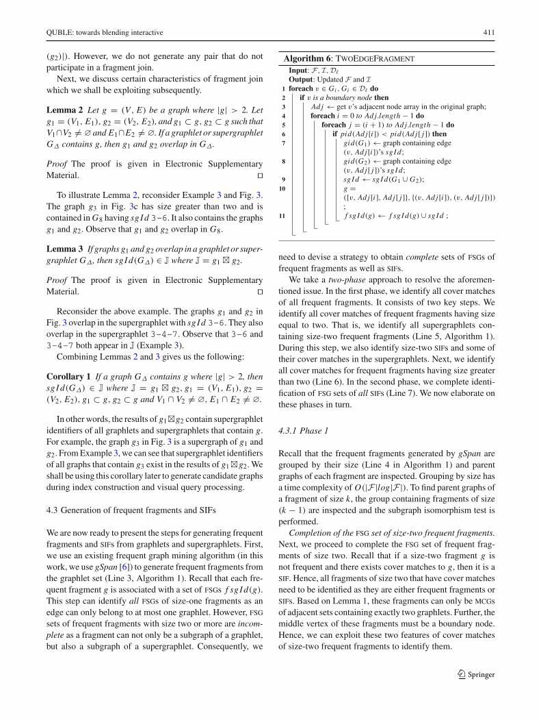
Example 5 Consider the frequent fragments f1, f2, and f3

in Fig. 5a. Algorithm 6 computes the complete fsg sets off1 and f2 ( f sgI d( f1) ={4–7, 3–6, 2} and f sgI d( f2) ={2,3,4}). gSpan computes f sgI d( f3) = {2}, which doesnot identify all occurrences of f3 in the original network.Hence, Algorithm 7 is invoked to compute the complete fsg

set of f3. Observe that | f1| = | f2| = 2 and | f3| = 3. Hence,they belong to groups F2 and F3, respectively. Since f1 andf2 are subgraphs of f3 (Line 5), their f sgI ds are addedinto cand Sets (Line 6). As f3 only has two parent graphs,f sgI d( f1) and f sgI d( f2) are selected and the fragment joinof f1 and f2 is computed (Lines 7–8). This results in J ={2,3–6, 4–7}. Hence, 2 is removed from J (Line 9). Next,supergraphlets with sgI ds 3–6 and 4–7 are loaded fromDΔ (Lines 11–15). Because they both contain f3, their sgI dsare added into f sgI d( f3) (Lines 16–17) and the algorithmterminates. Hence, f sgI d( f3) ={2, 4–7, 3–6}.

123


Fig. 5 Frequent fragments andsifs

(a)

(b)

4.3.2 Phase 2

Notice that in Phase 1, we have also identified all sifs of sizetwo and their cover matches, but their fsg sets are partiallycomplete. In this phase, we shall identify size-one sifs andcomplete fsg identifier sets of sifs of all sizes.

Algorithm 8 outlines the procedure to identify fsg iden-tifiers of sifs of all sizes. Note that size-one sifs can beretrieved from the set of graphlets (D�). For each edge, ifit is a sif (not in F), then it is added to the sif set I andsgI d of the graphlet containing it is inserted into the corre-sponding f sgI d set (Lines 1–3). The time complexity of thisstep is O(|E |). Notice that as a single edge cannot belong totwo graphlets, f sgI ds of size-one sifs do not contain anysupergraphlet identifier.

We have already identified size-two sifs and their covermatches using Algorithm 6. However, they may also occur assubgraphs in graphlets. To identify these occurrences in orderto complete the fragments’ f sgI d set, first the candidategraphlets are identified (Lines 4–7). Specifically, the candi-date set is generated as follows: cand I d(g) = f sgI d(g1)∩f sgI d(g2) where g1 and g2 are size-one subgraphs of frag-ment g. Since a size-one fragment is either a frequent frag-ment or a sif, the f sgI d sets have already been constructedearlier. Hence, we do not need to scan the database again toobtain cand I d(g). Next, the subgraph isomorphism test isperformed on these candidate graphlets, and identifiers of thematched results are added to f sgI d(g) (Lines 8–11).

Example 6 Consider the three sifs in Fig. 5b. Their f sgI dsbefore invoking Algorithm 8 are f sgI d(si f1) = {1,4}, f sgI d(si f2) = {2,4,5}, and f sgI d(si f3) ={1–5}. Sincesi f1 and si f2 are subgraphs of si f3, cand I d(si f3) can becomputed as f sgI d(si f1) ∩ f sgI d(si f2) = {4}. Since G4

contains si f3, 4 is added to f sgI d(si f3). Hence, the com-plete f sgI d(si f3) is {1–5, 4}.

4.4 Index construction

After generating complete sets of fsg identifiers, we can nowadopt the action-aware indices of prague [8,9] for indexingthe frequent fragments and sifs. The structure of the indicesand algorithms to generate them are identical to the onesdescribed in [8]. For the sake of completeness, we brieflydescribe them here.

Algorithm 8: CompleteSIF

Input: sif set I,D�

Output: Updated Iforeach edge g ∈ D� do1

if | f sgI d(g)| < α|D�| then2I ← (cam(g), f sgI d(g));3

foreach fragment g ∈ I where |g| = 2 do4Identify g’s two edges g1, g2;5Load f sgI d(g1), f sgI d(g2) from F or I;6cand I d(g)← f sgI d(g1) ∩ f sgI d(g2);7foreach sgI d(GΔk ) ∈ cand I d(g) do8

Load corresponding graph G� from D�;9if verify(g,G�) then10

Add sgI d(G�) to f sgI d(g);11

The action-aware frequent index (a2f) is a graph-struc-

tured index having a memory-resident and a disk-residentcomponents called memory-based frequent index (mf-index)and disk-based frequent index (df-index), respectively.Small-sized frequent fragments (frequently utilized) arestored in a mf-index, whereas larger frequent fragments (lessfrequently utilized) reside in a df-index. Informally, a df-index is an array of fragment clusters. A fragment cluster isa directed graph C = (VC , EC ) where each vertex8 v ∈ VC

is a frequent fragment g where the size of g (denoted as | f |)is greater than the fragment size threshold β (i.e., |g| > β).There is an edge (v′, v) ∈ EC iff g′ is a proper subgraph of g(denoted as g′ ⊂ g) and |g| = |g′| + 1. The root vertex (ver-tex with no incoming edge) of C is denoted by root (C). Eachfragment g of v is represented by its cam code [6]. Each ver-tex with fragment g in C points to a set of fsg identifiers ofg. Note that given the frequent fragments g and g′, if g′ ⊂ gthen f sgI d(g)∩ f sgI d(g′) = f sgI d(g) [2]. Hence, a ver-tex with fragment g stores only the f sgI d that are not sharedwith its children (denoted by del I d(g) ⊂ f sgI d(g)).

An mf-index indexes all frequent fragments having sizeless than or equal to β. Similar to a fragment cluster, it isa directed graph G M = (VM , EM ) where the vertices andedges have same semantics as C. In addition, by abusingnotations for trees, vertices representing frequent fragmentsof size β are leaf vertices in G M . Each leaf vertex v ∈ VM

(representing f ) is additionally associated with a fragment

8 For clarity, we distinguish between a node in a query (data) graphfragment and a node in action-aware indexes and g- spigs by using theterms “node” and “vertex”, respectively.

123


cluster list L where each entry Li points to a fragment clus-ter C j in the df-index such that g ⊂ root (C j ). Also, eachvertex v in the a

2f-index is assigned an identifier, denoted

by a2 f I d(v).The action-aware infrequent index (a2

i) indexes sifs toprune the candidate space for infrequent queries. It consistsof an array of sifs arranged in ascending order of their sizes.Each entry stores the cam code of a sif g and a list of fsg

identifiers of g. The identifier of each sif g in the index isdenoted by a2i I d(g).

5 Graphlet-based SPIG

Spindle-shaped graphs (spig) have been successfully exploi-ted in generating exact and similar subgraph candidates inprague [9]. Hence, we utilize this idea and create a variantof it called graphlet-based spig (g- spig) to suit the goalof finding exact and similar matches in the context of largegraphs. We first briefly describe the structure of a g- spig andhighlight its differences with spig [9]. Next, we describe thealgorithm for constructing a g- spig.

5.1 Structure of G-SPIG

For each new edge em created by a user, similar to prague [9],quble creates a graphlet-based spindle-shapedgraph (g-

spig). Each edge is assigned a unique identifier according toits formulation sequence. That is, the mth edge constructedby a user is denoted as em where m is the label of the edge.The edge with the largest m is referred to as new edge.

Similar to spig, a g- spig is also a directed graph Sm =(Vm, Em)where each vertex v ∈ Vm represents a subgraph gof a query fragment containing the new edge em . In the sequel,we refer to a vertex v and its associated query fragment ginterchangeably. There is a directed edge from a vertex v′ toa vertex v if g′ ⊂ g and |g| = |g′| + 1. Hence, vertices thatrepresent subgraphs of same size belong to the same level.The source vertex (vertex with no incoming edge) in the firstlevel of Sm , denoted by Sm .vsource, represents em and thetarget vertex (vertex with no outgoing edge) in the last level,denoted by Sm .vtarget , represents the entire query fragmentat a specific step.

The content of v in a g- spig is different from a spig.Specifically, each v is associated with the cam code [6] of thecorresponding g (denoted by cam(g)), a list of labels of edgesof g (denoted by LE (g)), a list of identifier set called IndexedFragments List, denoted by Lind(g), to capture informationrelated to frequent or infrequent nature of g or its subgraphs,and a set of identifiers Ω(g) called supergraphlet id set tohold the sgI ds of candidate graphlets and supergraphlets thatmay contain g, if g is not indexed by action-aware indices(i.e., g is a nif).

(a)

(c) (b)

Fig. 6 Visual query formulation

An Indexed Fragment List Lind(g) = ( f req I d(g), si fI d(g)) contains two attributes, namely frequent id ( f req I d(g)) and sif id (si f I d(g)). If g is in the a

2f-index or a

2i-

index, then the identifier of the vertex or entry v repre-senting g in the corresponding index is stored in the fre-quent id or sifid attribute, respectively (i.e., f req I d(g) =a2 f I d(g) and si f I d(g) = ∅ or si f I d(g) = a2i I d(g) andf req I d(g) = ∅, respectively).

If g is neither in the a2f-index nor in the a

2i-index (i.e.,

f req I d(g) = si f I d(g) = ∅), then the supergraphlet idset Ω(g) stores J = gv1 � gv2 where gv1 and gv2 are anytwo fragments associated with two different parents of v. Ifgv1 or gv2 is in the a

2f-index or a

2i-index, then their corre-

sponding f sgI ds are retrieved from these indices to com-pute J. Otherwise, supergraphlet id sets of the two parents(Ω(gv1) andΩ(gv2)) are used to computeΩ(g). Notice thatwe can always find two subgraphs to computeΩ(g) becauseall edges are either a frequent fragment or a sif. Hence, a nif

has size of at least two and has at least two parent graphs.

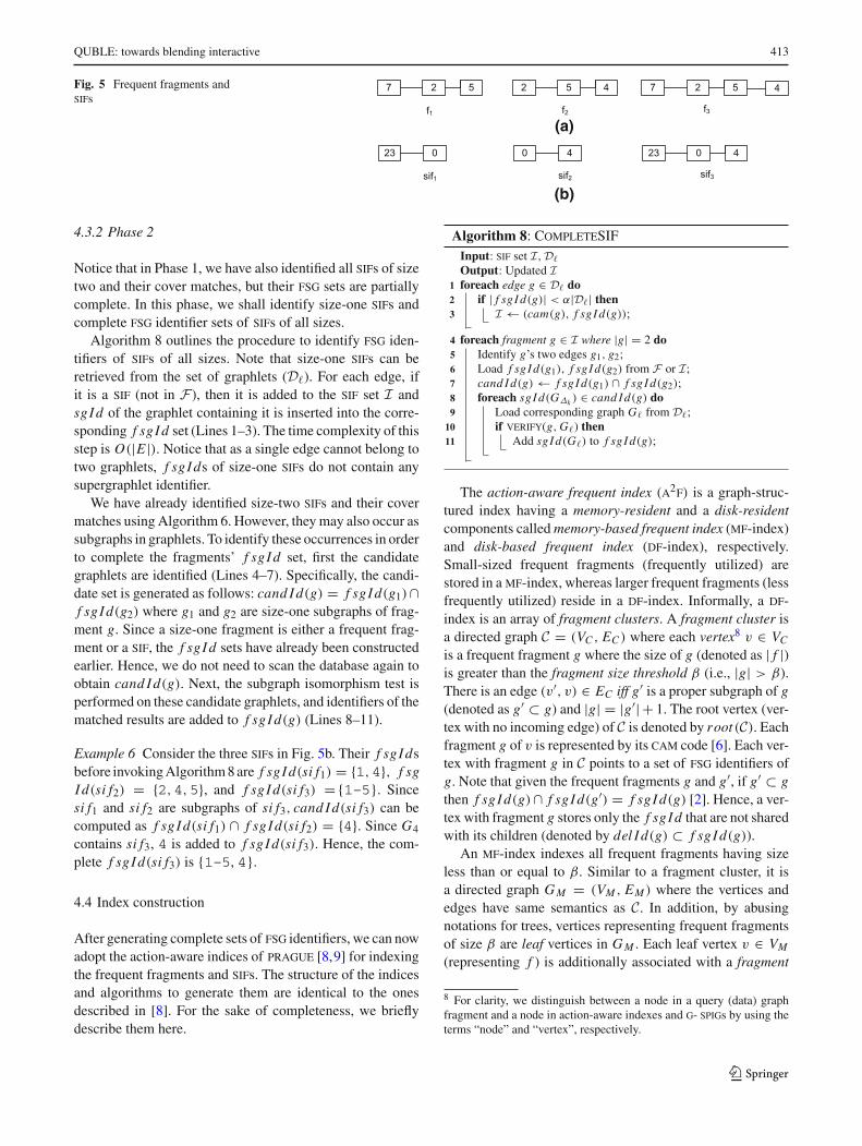
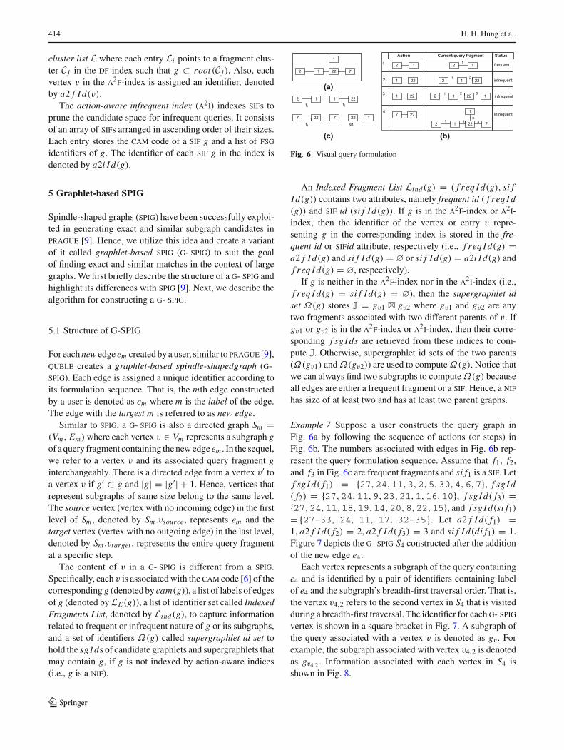
Example 7 Suppose a user constructs the query graph inFig. 6a by following the sequence of actions (or steps) inFig. 6b. The numbers associated with edges in Fig. 6b rep-resent the query formulation sequence. Assume that f1, f2,and f3 in Fig. 6c are frequent fragments and si f1 is a sif. Letf sgI d( f1) = {27,24,11,3,2,5,30,4,6,7}, f sgI d( f2) = {27,24,11,9,23,21,1,16,10}, f sgI d( f3) ={27,24,11,18,19,14,20,8,22,15}, and f sgI d(si f1)

={27–33, 24, 11, 17, 32–35}. Let a2 f I d( f1) =1, a2 f I d( f2) = 2, a2 f I d( f3) = 3 and si f I d(di f1) = 1.Figure 7 depicts the g- spig S4 constructed after the additionof the new edge e4.

Each vertex represents a subgraph of the query containinge4 and is identified by a pair of identifiers containing labelof e4 and the subgraph’s breadth-first traversal order. That is,the vertex v4,2 refers to the second vertex in S4 that is visitedduring a breadth-first traversal. The identifier for each g- spig

vertex is shown in a square bracket in Fig. 7. A subgraph ofthe query associated with a vertex v is denoted as gv . Forexample, the subgraph associated with vertex v4,2 is denotedas gv4,2 . Information associated with each vertex in S4 isshown in Fig. 8.

123


7 224

f3[V4,1]

7 224

sif1[V4,2] 13

7 224

sif1[V4,3] 12

1 222

inf1[V4,4] 74

13

2 1 2

inf2

[V4,5] 224

71

2 1 2 inf3[V4,6] 224

71

1

3

Fig. 7 A g- spig

Fig. 8 Information associated with the g- spig in Fig. 7

The first entry in the Indexed Fragment List refers tof req I d while the other refers to si f I d of the vertex. Sincev4,4 is a nif, we need to calculate its supergraphlet identi-fier set. Specifically, we need to retrieve f sgI d(gv4,2) andf sgI d(gv4,3) and compute gv4,2 � gv4,3 . Since gv4,2 and gv4,3

are sifs, f sgI d(gv4,2) = f sgI d(gv4,3) = f sgI d(si f1) andis retrieved from the a

2i-index. Hence, Ω(v4,4) ={27–33,

24, 11, 17, 32–35}. Similarly, we can compute Ω(gv4,5).Notice that gv4,5 has only one parent gv4,3 . In this case,we use v2,2 (of S2) which is not a vertex of S4 but is alsoassociated with a parent graph of gv4,5 to compute Ω(gv4,5)

(for reasons discussed later). Since gv2,2 is a nif, we useΩ(gv2,2) = gv1,1 � gv2,1 to compute gv2,2 � gv4,3 wheregv1,1 and gv2,1 represent f1 and f2, respectively. Hence,Ω(gv2,2) = {27,24,11}. Since gv4,3 is si f1, so f sgI d(si f1)

is used in computing this fragment join. Hence, Ω(gv4,5) =gv2,2 �gv4,3 ={27–33, 24, 11}. Lastly for gv4,6 , since it is anif along with gv4,4 and gv4,5, Ω(gv4,4) andΩ(gv4,5) are usedto calculate Ω(gv4,6) = gv4,4 � gv4,5 ={27–33, 24, 11}.

5.2 Algorithm

Algorithm 9 outlines the g- spig construction procedure. Thebuilding process starts from a new edge em (Lines 1–3). Itfirst attaches the cam code [6] and edge label of em to thevertex vm,1 of Sm and is enqueued in the vertex queue Q. Letvm,i be a vertex dequeued from Q (Line 5). If the graph gvm,i

associated with vm,i is a frequent fragment or sif, its fre-quent id or sif id will be attached to vm,i , respectively (Line

Algorithm 9: GSpigConstruct

Input: Query q, Vertex queue Q, new edge em , set of g- spigs S

Output: Graphlet-based spindle-shaped graph Smvm,1 ← f (em);1Enqueue(vm,1,Q);2Insert(vm,1, Sm);3while Q �= ∅ do4

vm,i ← Dequeue(Q);5

if gvm,i ∈ a2f-index or a

2i-index then6

Attach vm,i with si f I d(gvm,i ) or f req I d(gvm,i );7else8

Find vm, j1, vm, j2 in Sm that are parents of vm,i ;9if vm, j2 does not exist then10

g′i ← gvm,i − em ;11

gvm, j2 ← Search cam(g′i ) in the |g′i |-th level of other12S′k ∈ S;

Ω(vm,i )← gvm, j1 � gvm, j2 ;13

if |gvm,i |=|q| then14Add Sm in S;15return Sm ;16

else17foreach gvm,i ⊂ gvm, j ⊆ q and |gvm, j |=|gvm,i |+118

doif vm, j �∈ Q then19

vm, j ← f (gvm, j );20

Enqueue(vm, j ,Q);21Insert(vm, j , Sm);22

Connect edge(vm,i , vm, j );23

7). If gvm,i is a nif, the algorithm needs to find two verticesvm, j1, vm, j2 in Sm that are parents of vm,i (Line 9). Eventhough gvm,i always has at least two subgraphs whose sizesare |gvm,i | − 1, not all of them contain the new edge em (e.g.,gv4,5 ). Hence, their associated v may not belong to Sm . Con-sequently, if we can only find one parent of vm,i (there mustbe at least one incoming edge to vm,i because only the sourcevertex in Sm has no incoming edge), then first a subgraph g′ican be constructed by removing em from gvm,i (e.g., removee4 from gv4,5 in Example 7). Next, the algorithm seeks g′i ’sassociated vertex v in the |gi |th level of another g- spig in Sas the second parent of gvm,i (e.g., gv2,2 in S2) (Lines 10–12).Note that vertices in a g- spig that represent subgraphs ofthe same size belong to the same level. Upon obtaining twoparents, gvm, j1 and gvm, j2 , the algorithm generates the super-graphlet id set of gvm,i by computing fragment join of theseparent graphs (Line 13). When |gvm,i | = |q|, the construc-tion of Sm is completed and it is added to the g- spig set S(Lines 14–15). Otherwise, the vertex vm, j is constructed as achild of vm,i in Sm . For each gvm, j ⊃ gvm,i in q, if vm, j doesnot exist in Q, then it attaches the cam code and edge labelsof g j to vm, j and inserts the vertex into Q. Lastly, it addsvm, j into Sm and constructs a directed edge from vm, j to vm,i

(Lines 18–23). Fig. 9 depicts the set of g- spigs created bythis algorithm for the query graph in Fig. 6a.

123


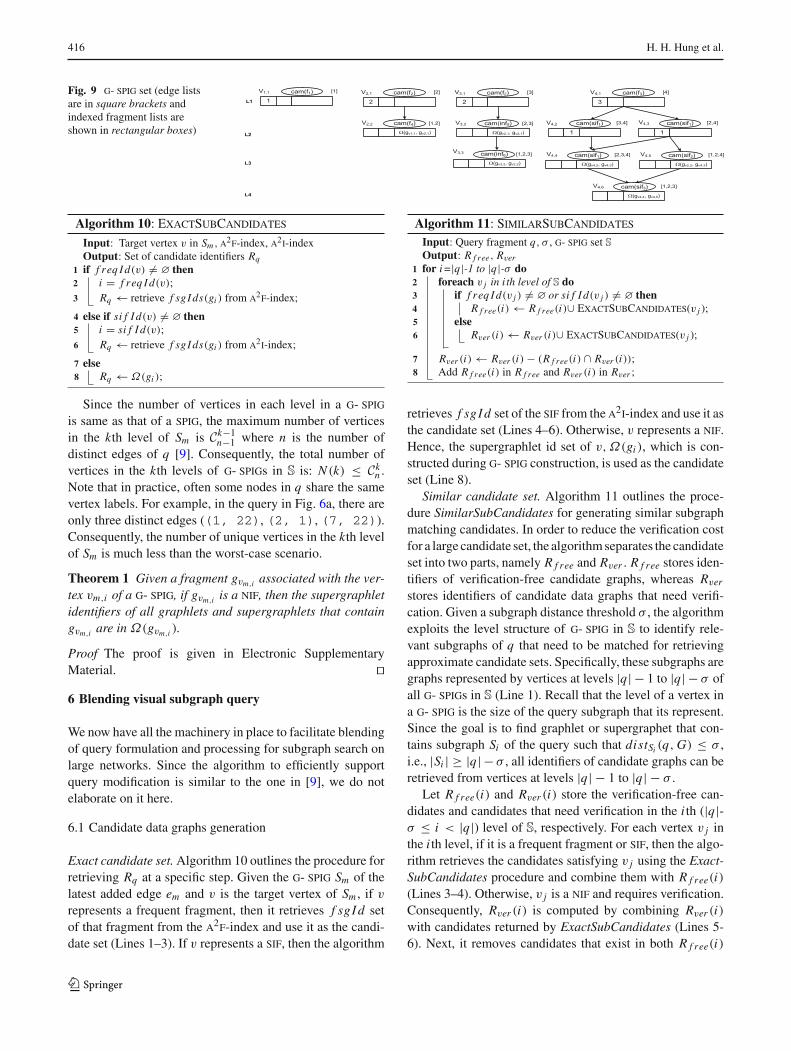
Fig. 9 g- spig set (edge listsare in square brackets andindexed fragment lists areshown in rectangular boxes)

Algorithm 10: ExactSubCandidates

Input: Target vertex v in Sm ,a2f-index, a

2i-index

Output: Set of candidate identifiers Rqif f req I d(v) �= ∅ then1

i = f req I d(v);2

Rq ← retrieve f sgI ds(gi ) from a2f-index;3

else if si f I d(v) �= ∅ then4i = si f I d(v);5

Rq ← retrieve f sgI ds(gi ) from a2i-index;6

else7Rq ← Ω(gi );8

Since the number of vertices in each level in a g- spig

is same as that of a spig, the maximum number of verticesin the kth level of Sm is Ck−1

n−1 where n is the number ofdistinct edges of q [9]. Consequently, the total number ofvertices in the kth levels of g- spigs in S is: N (k) ≤ Ck

n .Note that in practice, often some nodes in q share the samevertex labels. For example, in the query in Fig. 6a, there areonly three distinct edges ((1, 22), (2, 1), (7, 22)).Consequently, the number of unique vertices in the kth levelof Sm is much less than the worst-case scenario.

Theorem 1 Given a fragment gvm,i associated with the ver-tex vm,i of a g- spig, if gvm,i is a nif, then the supergraphletidentifiers of all graphlets and supergraphlets that containgvm,i are in Ω(gvm,i ).

Proof The proof is given in Electronic SupplementaryMaterial. ��6 Blending visual subgraph query

We now have all the machinery in place to facilitate blendingof query formulation and processing for subgraph search onlarge networks. Since the algorithm to efficiently supportquery modification is similar to the one in [9], we do notelaborate on it here.

6.1 Candidate data graphs generation

Exact candidate set. Algorithm 10 outlines the procedure forretrieving Rq at a specific step. Given the g- spig Sm of thelatest added edge em and v is the target vertex of Sm , if vrepresents a frequent fragment, then it retrieves f sgI d setof that fragment from the a

2f-index and use it as the candi-

date set (Lines 1–3). If v represents a sif, then the algorithm

Algorithm 11: SimilarSubCandidates

Input: Query fragment q, σ , g- spig set S

Output: R f ree, Rverfor i=|q|-1 to |q|-σ do1

foreach v j in i th level of S do2if f req I d(v j ) �= ∅ or si f I d(v j ) �= ∅ then3

R f ree(i)← R f ree(i)∪ ExactSubCandidates(v j );4else5

Rver (i)← Rver (i)∪ ExactSubCandidates(v j );6

Rver (i)← Rver (i)− (R f ree(i) ∩ Rver (i));7Add R f ree(i) in R f ree and Rver (i) in Rver ;8

retrieves f sgI d set of the sif from the a2i-index and use it as

the candidate set (Lines 4–6). Otherwise, v represents a nif.Hence, the supergraphlet id set of v,Ω(gi ), which is con-structed during g- spig construction, is used as the candidateset (Line 8).

Similar candidate set. Algorithm 11 outlines the proce-dure SimilarSubCandidates for generating similar subgraphmatching candidates. In order to reduce the verification costfor a large candidate set, the algorithm separates the candidateset into two parts, namely R f ree and Rver . R f ree stores iden-tifiers of verification-free candidate graphs, whereas Rver

stores identifiers of candidate data graphs that need verifi-cation. Given a subgraph distance threshold σ , the algorithmexploits the level structure of g- spig in S to identify rele-vant subgraphs of q that need to be matched for retrievingapproximate candidate sets. Specifically, these subgraphs aregraphs represented by vertices at levels |q| − 1 to |q| − σ ofall g- spigs in S (Line 1). Recall that the level of a vertex ina g- spig is the size of the query subgraph that its represent.Since the goal is to find graphlet or supergraphet that con-tains subgraph Si of the query such that distSi (q,G) ≤ σ ,i.e., |Si | ≥ |q| − σ , all identifiers of candidate graphs can beretrieved from vertices at levels |q| − 1 to |q| − σ .

Let R f ree(i) and Rver (i) store the verification-free can-didates and candidates that need verification in the i th (|q|-σ ≤ i < |q|) level of S, respectively. For each vertex v j inthe i th level, if it is a frequent fragment or sif, then the algo-rithm retrieves the candidates satisfying v j using the Exact-SubCandidates procedure and combine them with R f ree(i)(Lines 3–4). Otherwise, v j is a nif and requires verification.Consequently, Rver (i) is computed by combining Rver (i)with candidates returned by ExactSubCandidates (Lines 5-6). Next, it removes candidates that exist in both R f ree(i)

123


and Rver (i) from Rver (i) as these are already identified asverification-free candidates (Line 7). Finally, it adds Rver (i)and R f ree(i) in Rver and R f ree, respectively.

Example 8 Reconsider the formulation sequence of thequery in Fig. 6 and the corresponding g- spig set in Fig. 8.Suppose σ = 2. When the first edge is added, g- spig S1

is constructed (Line 3, Algorithm 2). The target vertex v1,1

is passed as input to invoke Algorithms 10 and 11, respec-tively (Lines 4–5, Algorithm 2). In Algorithm 10, sincef req I d(v1,1) = 1, the identifier of fragment gv1,1 associ-ated with v1,1 is retrieved (Lines 1–2). Based on the identi-fier, the corresponding f sgI d set is retrieved from the a

2f-

index and assigned to Rq (Line 3). Next, in Algorithm 11, as|q| = 1, Rq remains unchanged.

When the second edge is added, S2 is constructed and thetarget vertex is now v2,2. Algorithms 10 and 11 are invoked.Since f req I d(v2,2) = si f I d(v2,2) = ∅,Ω(gv2,2) =gv1,1 � gv1,2 , which has already been computed duringthe construction of S2. Hence, it is assigned to Rq . InAlgorithm 11, as |q| = 2, vertices at level i = |q| −1 = 1 of the g- spig set are considered (i.e., verticesv1,1 and v2,1). Since f req I d(v1,1) = 1, f sgI d(gv1,1) ={27,24,11,3,2,5,30,4,6,7} (Example 7) is retrievedfrom the a

2f-index and added into R f ree(1) (Lines 3-

4). Similarly, f req I d(v2,1) = 2 and f sgI d(gv2,1) ={27,24,11,9,23,21,1,16,10} is retrieved and addedinto R f ree(1) set. After this step, Rver is empty andR f ree(1) = {27,24,11,3,2,5,30,4,6,7,11,9,23,21,1,16,10} is added into R f ree (Line 8).

S3 is constructed with the addition of the third edge.Hence, v3,3 is now the target vertex. Since f req I d(v3,3) =si f I d(v3,3) = ∅, Ω(gv3,3) = gv3,2 � gv2,2 , which hasalready been computed earlier, is assigned to Rq . As |q| = 3,vertices from level two to one (i.e., v2,2, v3,2, v1,1, v2,1

and v3,1) of the g- spig set are considered. When leveli = 2, f req I d(v2,2) = si f I d(v2,2) = ∅,Ω(gv2,2) =gv1,1 � gv2,1 = {27,24,11} is added into Rver (2) (Line6, Algorithm 11). Also, f req I d(v3,2) = si f I d(v3,2) =∅,Ω(gv3,2) = gv2,1 � gv3,1 = {27,24,11,9,23,21,1,16,10} is added into Rver (2), which is inserted into Rver

after executing Line 8. For i = 1, f sgI d(gv2,1) andf sgI d(gv1,1) are added into R f ree(1) in the same way as dis-cussed in Step 2. Since f req I d(v3,1) = 1, f sgI d(gv3,1) ={27,24,11,9,23,21,1,16,10} is retrieved by probingthe index and added into R f ree(1). Subsequently, R f ree(1) ={27,24,11,3,2,5,30,4,6,7,11,9,23,21,1,16,10} is added into R f ree.

Finally, S4 with the target vertex v4,6 is constructedafter the addition of the last edge. Since f req I d(v4,6) =si f I d(v4,6) = ∅,Ω(gv4,6) = gv4,4�gv4,5 = {27− 33,24,11} is assigned to Rq . As |q| = 4, vertices from leveli = |q| − 1 = 3 to i = |q| − σ = 2 of S are con-

Algorithm 12: ExactVerification

Input: Query q, Rq , g- spig set S,DΔ

Output: ResultsSm ← the newest g- spig in S;1v← Sm,vtarget ;2

if f req I d �= ∅ or si f I d �= ∅ then3Results ← Rq ;4

else5foreach sgI di in Rq do6

if graph GΔ with sgI di already been constructed in DΔ7then

Load GΔ from DΔ;8else9

GΔ ← SupGraphletConst(sgI di ,D�) /*10Algorithm 4 */;Add GΔ into DΔ;11

if verify(q,GΔ) then12Add sgI d(GΔ) into Results;13

sidered (i.e., v3,3, v4,4, v4,5, v2,2, v3,2, v4,2, and v4,3). Fori = 3, frequent ids and sif ids of v3,3, v4,4, and v4,5 areempty. Hence, their supergraphlet id sets are added intoRver (3). Consequently, Rver (3) ={27–33, 24, 11, 17,32–35, 27} is added into Rver . For i = 2, si f I d(v4,2) =si f I d(v4,3) = 1, so f sgI d(gv4,2) = f sgI d(gv4,3) =f sgI d(si f1) ={27–33, 24, 11, 17, 32–35} are addedinto R f ree(2). Since frequent ids and sif ids of both v2,2 andv3,2 are empty, Ω(gv2,2) = {27,24,11} and Ω(gv3,2) ={27,24,11,9,23,21,1,16,10} are added into Rver (2).Also, R f ree(2) ={27–33, 24, 11, 17, 32–35} andRver (2) = {27,24,11,9,23,21,1,16,10}. Hence, thecommon values {24, 11} of R f ree(2) and Rver (2) areremoved from Rver (2) (Line 7, Algorithm 11). Hence, finallyR f ree(2) ={27–33, 24, 11, 17, 32–35} and Rver (2) ={27,9,23,21,1,16,10} are added into R f ree and Rver ,respectively (Line 8).

6.2 Generation of query results

Exact subgraph matching results computation. The proce-dure for exact subgraph candidate verification is reported inAlgorithm 12. If the final query is a frequent fragment or asif, the current exact subgraph candidate identifiers do notneed verification and can be returned immediately as the finalresult (Lines 3–4). If the final query is a nif, verification isrequired (Lines 6–13). Notice that if a sgI d in the candi-date set does not exist in DΔ, Algorithm 4 will be invoked toconstruct the supergraphlet before verification is performed.

Similar subgraph matching results computation. Algo-rithm 13 outlines the procedure for generating ordered queryresults containing approximate matches. As the subgraphdistance of candidate graphs associated with the i th levelof g- spigs in S is |q| − i , the higher level the candidategraph is in S, the more similar it is to the query graph. Ateach level i from |q| − 1 to |q| − σ in S, verification-free

123


Algorithm 13: SimilarResultsGen

Input: q, R f ree, Rver and σ , g- spig set S

Output: Ordered result set Resultsfor i=|q|-σ to |q|-1 do1

Results ← Results ∪ R f ree(i);2Rver (i)← Rver (i) ∩ Results;3for each candidate graphlet c in Rver (i) do4

if SimVerify(q, S, c, |q| − i) is T rue then5Results ← Results ∪ {c};6

candidates (R f ree(i)) are added first in Results (Line 2).Then, the elements in Rver (i) that already exist in Resultsare removed from Rver (i) (Line 3). This step is necessarybecause at lower levels, some data graph sgI ds have alreadybeen verified and added to Results at previous higher levels.As such, they need to be removed from current Rver (i) toavoid duplicate verification. Next, each candidate elementin Rver (i) is verified by SimVerify procedure [9] to obtainthe result set to be added into Results (Lines 5–6). Note thatSimVerify extends VF2 [3] and exploits the g- spigs to han-dle mccs-based similarity verification (See Electronic Sup-plementary Material for pseudocode). In order to facilitateretrieval of all matches in a supergraphlet (discussed below), we also store the states of VF2 at termination.

Computation of all matches in a given supergraphlet.Recall that in our visual paradigm, a user may select a result(super)graphlet GΔ to initiate viewing all matches (bothexact and approximate) to the query graph in GΔ. We againexploit the g- spig of q and invoke the VF2 algorithm [3]multiple times for each subgraph of q whose distance is notlarger than σ . Since this process can produce some redun-dant matches, we filter them using a subset-inclusion test.Note that we do not need to find approximate matches start-ing from σ = 0 as we can leverage previously computedstates of VF2 at termination (by the SimVerify procedure).The formal pseudocode is given in Electronic Supplemen-tary Material.

Remark Note that our focus here is not to develop an efficientsimilar subgraph verification technique for large networks. Infact, we can easily replace the implementation of SimVerifywith a more efficient one without modifying the frameworkof quble. Similarly, since the size of a graphlet (controlledby the partition threshold) is significantly smaller than theoriginal network in quble to facilitate effective result visual-ization, we use the aforementioned simple strategy to effec-tively compute all matches. Fortunately, in spite of usingsuch simple techniques, quble has very good performanceas demonstrated in Sect. 7.

7 Performance study

quble is implemented in Java jdk 1.7. We run all experi-ments on an Intel Xeon X5570 2.93 GHz machine running

Table 2 Datasets

on Windows 7 × 64 with 12 GB ram. Note that there is noexisting system that realizes our new visual subgraph queryparadigm on large networks. Nevertheless, since one of ourgoal is to demonstrate that our proposed paradigm does notsacrifice system response time compared to the traditionalparadigm, we confine ourselves to compare quble (denotedby qub for brevity) against sapper (denoted by sap) forselective9 experiments. We obtain the binary code of sap

from the authors of [19].

7.1 Experimental setup

Datasets. We use subsets of modified dblp co-authorshipdataset modeled as a graph where a node and an edge rep-resent an author and co-authorship, respectively. Since mostof the nodes are distinct author names, there are no frequentfragments. Hence, in order to investigate the effect of frequentas well as infrequent fragments, we map each node (author)to its degree and use it as its label. This generates at most300 distinct node labels. The characteristics of these datasetsare reported in Table 2. Note that recent subgraph similaritysearch techniques on large networks such as [12,19] haveused datasets containing at most 10k nodes.

Querysets. Since queries are formulated by end usersusing an “edge-at-a-time” visual interface, it is not realisticto expect a user to formulate large queries visually. There-fore, we chose query graphs having sizes of 4, 8, 12, 16,and 20 (Fig. 2 in Electronic Supplementary Material depictsthe queryset). All these queries are chosen as nifs as suchtype of queries demonstrate “worst” case performance ofqub. Recall from Sect. 6.2, frequent and sif queries do notneed expensive candidate verification as the results can beefficiently computed directly from action-aware indexes. Onthe other hand, nif queries are not indexed by our indexingschemes and require candidate verification. Besides, unliketraditional approaches [19] where the benchmark queries areautomatically generated from the graph database, the querieshere are visually formulated by real end users. Hence, it is notpossible to generate a large number of visual queries as ourpreliminary study revealed that such aspiration is not only

9 Recall that sapper [19] only retrieves similarity matches contain-ing same number of nodes as the query graph (Sect. 2.2). In contrast,qub allows retrieval of similar subgraphs that do not necessarily havethe same number of nodes as the query. Hence, candidate data graphsas well as result sets generated by these approaches are different andincomparable.

123


Table 3 α values

expensive, but also strongly deters end users to participatein the empirical study. Unless mentioned otherwise, we shallbe using the default sequence (see Electronic SupplementaryMaterial) for formulating a particular query.

Participants profile. Eight unpaid male volunteers (agesfrom 21 to 27) participated in the experiments. None of themare familiar with any graph query languages. They were firsttrained to use the gui of qub. For every query, participantswere given some time to determine the steps that are neededto formulate it visually. This is to ensure that the effect ofthinking time is minimized during query formulation. Notethat faster a user formulates a query, the lesser time qub

has for g- spig construction. Each query was formulated fivetimes by each participant, and reading of the first formulationwas ignored. The average query formulation time (qft) for aquery by all participants is given in Electronic SupplementaryMaterial.

Default parameter settings. We set σ = 4, β = 3, p = 50for qub and θ = 3 for sap unless specified otherwise. Wechose different values for α for different datasets (Table 3).This is because the number of graphlets varies greatly fordifferent datasets. For example, there are only 69 graphletsin d1k but 17716 in d100k dataset under default parametersettings. Therefore, in order to have a reasonable set of fre-quent fragments, we choose different α values. If the sameα is used for all datasets, the number of frequent fragmentswill be unnecessarily too high in small datasets or too smallin large datasets to be meaningful. The default α value is setto α1 in Table 3.

7.2 System response time (SRT)

We first investigate srts of qub for evaluating subgraph sim-ilarity queries by varying different parameters and compareit with sap. The average srt is computed by taking the aver-age of srts of all participants (last four formulations). Inthe sequel, the srt of qub refers to this average srt unlessspecified otherwise. Furthermore, we group the query setaccording to their sizes and srts of queries in each group areaveraged and recorded as the srt of that group size.

Figure 10 reports the srts for different query size. In sap,the srt refers to the query execution time. Each query wasexecuted five times, and results from the first run were alwaysdiscarded. Observe that qub performs significantly betterthan sap consistently across different query size for different

(a) (b)

(c) (d)

(e) (f)

Fig. 10 srts of quble and sapper (in log scale)

datasets. This is mainly because of qub’s approach of blend-ing query formulation with query processing. As sap failedto construct index for d100k in 3 h, we do not compare itwith qub for this dataset.

Effect of subgraph distance threshold. Recall that the def-inition of edge edit distance θ in sap is not compatible withour subgraph distance threshold σ . While qub allows bothedges and nodes to be missed (i.e., the node set of a matchcan be a subset of the query graph’s node set), edge edit dis-tance only allows edges to be missed (i.e., the node set of amatch must be exactly the same as that of the query graph).Besides, for an edge edit distance θ , if there is no subgraphof the query that has exactly θ edges less than the query andthe same node set, sap immediately terminates its search. So,a higher θ value may not return any result for some queries.Hence, we do not compare the srts of qub with sap underdifferent subgraph distance threshold values. Figure 11 plotssrts of qub for different σ values. Generally, srt increaseswith σ as more candidate graphs are generated when σ isrelaxed, allowing more approximate matches of the query.However, in some cases, it decreases with increase in σ asit is influenced by the processing order of vertices duringsubgraph verification. Importantly, the srts are cognitivelynegligible as typically it takes less than a second to viewquery results.

Effect of partition threshold. In Fig. 12, we study theeffect of partition threshold p on the srt. In most cases, weobserve an increasing trend in srt. This is because when pincreases, the size of candidate data graphs increases. Thus,it takes more time to perform subgraph isomorphism veri-fication on these candidate graphs. In some cases, we alsoobserve decreasing trend, due to decrease in the number of

123


(a) (b)

(c) (d)

(e) (f)

Fig. 11 Effect of σ

(a) (b)

(c) (d)

(e) (f)

Fig. 12 Effect of partition threshold on srt

candidate graphs. For a given dataset, when p increases, thenumber of graphlets decreases. This sometimes leads to adecrease in the number of candidate graphs.

Effect of the number of verification candidates. Figure 13depicts the number of verification candidates in qub andcorresponding srts of representative queries for different σvalues. We use the d100k dataset as it produces the high-est number of candidate graphs. We can make the follow-ing observations. In most cases, the srt is correlated to thenumber of candidate graphs that require verification. This is

0

10

20

30

40

50

01020304050607080

1 2 3 4

SR

T (

ms)

Ver

ific

atio

n C

and

idat

e

number of verification candidate SRT

051015202530

010203040506070

1 2 3 4

SR

T (

ms)

Ver

ific

atio

n C

and

idat

e


00.511.522.533.5

0

20

40

60

80

100

1 2 3 4

SR

T (

ms)

Ver

ific

atio

n C

and

idat

e


0

0.2

0.4

0.6

0.8

1

0

5

10

15

20

25

1 2 3 4

SR

T (

ms)

Ver

ific

atio

n C

and

idat

e


00.511.522.53

0

50

100

150

200

250

1 2 3 4

SR

T (

ms)

Ver

ific

atio

n C

and

idat

e number of verification candidate SRT

0

5

10

15

20

25

0500

1000150020002500300035004000

1 2 3 4

SR

T (

ms)

Ver

ific

atio

n C

and

idat

e number of verification candidate SRT

5Q(b)2Q(a)

(c) Q9

(e) Q12

(d) Q11

(f) Q14

Fig. 13 Number of verifications

because in qub when a user clicks Run, the candidate graphset has already been generated, and only verification needs tobe performed. Observe that the srt is not strictly proportionalto the number of verification candidates. This is because theverification algorithm employs state space pruning, whichin some cases reduces state space faster than in other cases.Lastly, observe the sharp increase in the srt for Q2. Thisis primarily due to the simple subgraph verification methodwe have used rather than qub’s candidates pruning ability.We expect qub’s performance to significantly improve if asuperior candidate verification algorithm is adopted.

Effect of α and β. Figures 14 and 15 demonstrate theeffect of α and β on the srt, respectively. Overall, we donot observe any clear trend in the srt in relation to theseparameters. Importantly, srts of the queries are low for dif-ferent values of α and β.

Cost of all matches computation. We now measure thetime taken by qub to compute all matches when a user clickson a result graphlet. Specifically, given a query graph, wemeasure the maximal computation time (mct), which is thehighest time taken on any graphlet in the result set. That is,the mct represents the “worst-case” performance of a query.Figure 16a depicts the mcts of six representative queriesacross different values of σ . Clearly, the mct increases whenσ increases since larger σ implies that qub generates moreapproximate matches. Importantly, although we use a simplestrategy for computing all matches, the mct is still below onesecond which is cognitively negligible.

7.3 Index construction

Index size comparison. We study effects of various parame-ters on index size. Note that the publicly available executable

123


(a) (b)

(c) (d)

(e) (f)

Fig. 14 Effect of α

(a) (b)

(c) (d)

(e) (f)

Fig. 15 Effect of β

file of sap does not store indices back to the disk afterconstruction and terminates right after processing the queryinput. Hence, we are unable to compare the index size of qub

with sap.Due to the definition of sif, the number of sifs in each

dataset is typically much larger compared to the number of

(a) (b)

Fig. 16 Performance of computing all matches a DBLP (p = 50), bYoutube (p = 300)

Table 4 Index size (mb)

(a) (b)

(c) (d)

(e) (f)

Fig. 17 Effect of sifs

frequent fragments. As such, the number of sifs is an impor-tant factor contributing to index size. Hence, we study effectsof the number of nodes, p, and α on the number of sifs. Notethat β does not influence the number of sifs.

Table 4 and Fig. 17a report effects of the number of nodeson index size and the number of sifs, respectively. Fig-ures 17b–f plot effects of different parameters on index sizeand the number of sifs for different datasets. We can makethe following observations. First, there is an increasing trendin index size and the number of sifs when the number ofnodes increases. Second, both index size and the number ofsifs decrease when the partition threshold increases and isnot affected much by α and β. These observations can beexplained as follows.

• Given a partition threshold p, the number of graphletsincreases when the number of nodes in a dataset increases.Hence, for the same number of distinct labels, this

123


(b) Partition threshold

(c) Minimum support threshold (d) Fragment size threshold

(a) Number of nodes

0

20000

40000

60000

80000

100000

120000

50 75 100 200

Tim

e (m

sec)

Partition threshold

D1K D5K D10K

D20K D50K D100K

05000

10000150002000025000300003500040000

alpha1 alpha2 alpha3 alpha4

Tim

e (m

sec)

D1K D5K D10K

D20K D50K D100K

05000

10000150002000025000300003500040000

3 5 8 10

Tim

e (m

sec)

D1K D5K D10K

D20K D50K D100K

1

10

100

1000

10000

100000

D1K D5K D10K D20K D50K D100K

Tim

e (m

sec)

Datasets

Fig. 18 Index construction cost

increases the number of distinct size-one fragments andsize-two fragments that have cover matches. Conse-quently, the number of sifs and index size have increasingtrend.• For a given dataset, when p increases, the number of

graphlets decreases. There are fewer boundary nodes,and as a result, lesser size-two fragments that have covermatches. Therefore, we observe a decreasing trend.• Thresholds α and β do not affect index size and the num-

ber of sifs significantly as the number of frequent frag-ments in the mf-index in most datasets (except d1k whichhas more than 2,200 frequent fragments and 7,972 sifs) ismuch smaller than the number of sifs. Consequently, thevariance of frequent fragment number in this index doesnot affect index size significantly. Also, although when αincreases, the number of frequent fragments decrease andhence the number of sifs should increase, the increaseamount is small compared to the number of sifs. Hence,we do not observe a clear increasing trend.

Index construction cost. We now study the effect of num-ber of nodes and partition threshold on index constructiontime (Algorithm 1). Figure 18 depicts the index construc-tion cost of qub by varying different parameters. Observethat there is an increasing trend in the index constructiontime when the number of nodes increases. Similar trend isobserved for different partition thresholds. On the other hand,α and β do not influence the index construction time signif-icantly except for the d1k dataset, which has a decreasingtrend. These observations can be explained as follows.

First, the number of graphlets and boundary nodesincrease when the number of nodes increases. Consequently,as reported earlier, the number of sifs and index size increase.Because there are more information that need to be processed,the index construction time shows an increasing trend.

(a) (b)

(c) (d)

(e) (f)

Fig. 19 Steps in index construction

Second, for d1k dataset, the index construction time is rel-atively larger because of a large number of frequent frag-ments and clusters in the df-index that need to be processed.It decreases when α or β increases because the number offrequent fragments decreases and there are lesser clusters toconstruct in the df-index when β increases.

Let us now investigate in detail the major steps of indexconstruction in qub. Reconsider Algorithm 1 for index con-struction. Once the partial set of frequent fragments are gen-erated using gSpan, it consists of the following key steps: (1)grouping frequent fragments according to their size (Line 4);(2) identification of size-two sifs and the complete fsg setof size-two frequent fragments (Line 5); (3) identification ofthe fsg set of frequent fragments having size greater than2 (Line 6); and (4) generation of complete fsg sets of size-two sifs (Line 7). Hence, we now report the performances ofthese four steps during index construction.

Figure 19 reports the execution time of these four stepsfor different datasets and partition thresholds. For a givendataset, when the partition threshold p increases, the numberof graphlets decreases. There are lesser boundary nodes, andas a result, lesser size-two fragments that have cover matches.Consequently, there is a decreasing trend in the executiontime for Step 2. However, as p increases, the size of partitiongraphs increases. Hence, it takes more time to verify whethera partition graph contains a sif in Step 4. Thus, the timetaken to execute Step 4 increases. Observe that the increase inruntime of Step 4 offsets that of Step 2. Therefore, overall theindex construction time increases when p increases. Lastly,Steps 1 and 3 take significantly lesser time compared to Steps2 and 4 for all datasets except for d1k as it contains a largenumber of frequent fragments.

123


Fig. 20 Prefetching time andcost of fragment join (in ms.)

(a) (c)

(b) (d) (e)

7.4 Prefetching time

Recall that Algorithm 2 is invoked every time a new edgeis added during visual query formulation. Particularly, Lines2–5 are executed for each new edge. These steps involveconstruction of a g- spig and computation of candidate sets.Recall that during construction of a g- spig, we need to per-form fragment join to compute the candidate set if a fragmentis a nif (Line 13 in Algorithm 9). In this set of experiments,we investigate the computation time of fragment join oper-ation during query formulation as well as prefetching time(time to execute Lines 2–5 of Algorithm 2).

Prefetching time and fragment join cost. Figure 20 reportsthe prefetching time and fragment join cost. Observe that allprefetching times and fragment join execution times take lessthan 50 ms. Hence, both these operations are efficiently sup-ported in quble and takes cognitively negligible time. Noticethat the fragment join cost may be zero for the first two stepsin some queries as these edges are not nif and can be directlyretrieved using a

2f and a

2i-indexes. More importantly, since

the time taken to construct an edge in qub typically is at least2 s,10 prefetching step can easily be completed by exploitingthe gui latency.

Query formulation sequence. Since a visual query can beformulated by following different sequence of steps, differ-ent g- spig sets will be generated. We assess the effect of dif-ferent query formulation sequences on the prefetching timeand srt. Table 5 lists two different formulation sequencesfor representative test queries (we chose two representativequeries for each query size) and the average prefetching time(all participants) at different steps on d100k dataset. Observethat the prefetching operation for both sequences at each stepis very efficient and takes negligible time. It is significantlylower (almost an order of magnitude) than the available gui

latency of at least 2 s. Importantly, the formulation sequencesonly have minor effect on the prefetching time. Last but not

10 Here, we ignore the “user thinking time.” As the thinking timeincreases, the latency offered by a gui increases as well at each step.

the least, the impact of query formulation sequence on srtsis cognitively negligible for these queries highlighting therobustness of our technique.

7.5 Performance on a million-nodes network

In the preceding section, we have empirically demonstratedthe superiority of quble in processing subgraph queries onnetworks containing at most 100 K nodes. Although we use anetwork that is an order of magnitude larger than those usedin recent studies [12,19], today’s networks may have millionsof nodes (e.g., social networks). Can quble support subgraphsimilarity queries on such massive networks? In this section,we provide answer to this question affirmatively. Specifically,we use a Youtube social network graph11 where each noderepresents a user and each edge represents the friendshiprelation between two users. This network contains 1,157,827nodes and 2,987,624 edges. Similar to the dblp dataset, welabel each node using its degree which yields 979 uniquelabels. We chose 17 nif queries of sizes 4, 8, 12, 16, and 20(see Electronic Supplementary Material for details). Unlessspecified otherwise, we set α = 0.002, β = 3, σ = 4, andp = 300. Using this setting, we get 733,188 graphlets, 106frequent fragments, and 41,280,795 sifs. Since the number ofsifs is very large, the a

2i-index is stored in a rdbms (MySQL

Community Server 5.5) as it is too large to fit in the mainmemory. Specifically, the sizes of a

2f and a

2i indexes are

1.93mb and 23.86gb, respectively (the index constructioncost is given in Electronic Supplementary Material).

Effect of query size and σ on SRT. Figure 21a reports thesrt of qub for different query size. Expectedly, it increaseswith query size. Figure 21b depicts the srt across dif-ferent values of σ . Since larger σ leads to more approx-imate results which demands more verifications, the srt

increases with σ . Importantly, the srt is still below 5 s high-lighting the effectiveness of qub to handle million-nodesnetworks.

11 Downloaded from http://snap.stanford.edu/data/com-Youtube.html.

123

http://snap.stanford.edu/data/com-Youtube.html


Tabl

e5

Eff

ecto

fva

riat

ion

inqu

ery

form

ulat

ion

sequ

ence

(in

ms.

)

123


(a) (c) (d) (e)

(b) (f) (g)

Fig. 21 srts, Prefetching times, and cost of fragment join for the Youtube network (in ms)

Table 6 Effect of the formulation sequence (in ms.)

Computing all matches. Figure 16b depicts the averagemcts for computing all matches. We can make the follow-ing observations. First, for query size larger than 4, the mct

increases when the query size or σ increases. This is expectedas the number of approximate matches increases dramati-cally for these cases. Furthermore, larger queries also maylead to larger result (super)graphlets due to the fragment joinprocess. Second, the performance of size-4 queries does notchange significantly for larger σ . This is because the num-ber of approximate matches does not increase significantlyfor this case. Third and most importantly, even for a million-nodes network our simple all matches computation strategytakes only few seconds which we believe is acceptable in avisual querying environment.

Prefetching time and fragment join cost. Figures 21c–fplot the prefetching time and fragment join cost of qub.Observe that larger queries and latter steps tend to take moreprefetching time. It is expected as the core cost is the con-struction time of g- spig which grows for larger queries.

Nevertheless, even for the last step of a 20-edge query, theprefetching time is still within the latency offered by the gui

(at least 2 s). Additionally, similar to the dblp dataset, thefragment join operation is very efficient.

Query formulation sequence. Lastly, Table 6 lists three dif-ferent formulation sequences for representative test queriesand the average prefetching time (all participants) at differ-ent steps. Observe that the prefetching time and srt of allsequences are very efficient. That is, despite the increase innetwork size, the impact of query formulation sequence onsrts is cognitively negligible for these queries highlightingthe robustness of our paradigm.

8 Related work

Recently, there have been a number of studies to speed upevaluation of subgraph queries over large networks [5,12,13,18–20]. In contrast to quble, none of these strategies address

123


the subgraph query problem by partitioning a large networkinto small pieces. The indexing strategies do not exploit fre-quent and infrequent patterns for candidate pruning. Moreimportantly, all these efforts follow the conventional queryprocessing paradigm where the formulation of an entire querygraph precedes its evaluation. In contrast, in quble, queryprocessing is initiated when the entire query is not knownand leverages gui latency and users’ interaction behaviorsfor efficient pruning and retrieval. Nevertheless, quble isorthogonal to these traditional techniques.

More germane to this work is our previous efforts in [8,9],where we realized the new visual querying paradigm to sup-port subgraph queries on a large set of small or medium-sizedgraphs. Firstly, we focus on querying large networks hereinstead of a large set of small or medium-sized graphs. Sec-ondly, we use sifs instead of difs (discriminative infrequentfragments) as representative infrequent fragments. Note thatthe dif is either an infrequent fragment of size-one or it isa smallest infrequent subgraph of an infrequent fragment.On the other hand, a sif is either an infrequent fragment ofsize-one or it is a two-sized infrequent fragment and an mcg

of at least one adjacent set. Thirdly, the generation of fre-quent fragments and sifs are much more involved in quble.In [8,9], frequent fragments and difs can be directly gen-erated by using an existing frequent subgraph mining algo-rithm (executing only Line 3 in Algorithm 1). In contrast, inquble, the network needs to be decomposed into graphletsand supergraphlets (Lines 1–2), and then, they need to becarefully processed (Lines 4–7) to create approximate fre-quent fragment set and sifs. Fourthly, although the topolog-ical structure of a spig [9] and a g- spig is identical, thevertex content is different. In a g- spig, each vertex storesa set of (super)graphlet identifiers of (Ω(g)) and a sif idamong other features, which are irrelevant in a spig. Conse-quently, the construction algorithm of g- spig differs fromthe spig construction. Due to these differences, the candi-date generation process during query formulation also dif-fers. Lastly, visualization strategy of query results is differ-ent in quble due to the cognitive burden imposed by largenetworks.

9 Conclusions

In this paper, we have presented quble—a visual frame-work that supports processing of subgraph queries on largenetworks by blending their evaluation with visual query for-mulation. First, it decomposes a large network into a set ofgraphlets and supergraphlets using a minimum cut-basedgraph partitioning technique. Next, it mines approximate

frequent fragments and sifs from them and identifies theiroccurrences in the data graph. Once these fragments are-generated, quble extends the indexing framework of [9]to support efficient blending of visual subgraph query for-mulation and query processing. It also supports an interac-tive (super)graphlet-at-a-time results visualization schemeto provide a practical and effective visualization of queryresults. Exhaustive experimental studies on large networksvalidated the merit of quble.

References

1. Bhowmick, S.S. et al.: VOGUE: towards a visual interaction-awaregraph query processing framework. In: CIDR (2013)

2. Cheng, J., Ke, Y., Ng, W., Lu, A.: FG-Index: towards verification-free query processing on graph databases. In: SIGMOD (2007)

3. Cordella, L.P., Foggia, P., Sansone, C., Vento, M.: An improvedalgorithm for matching large graphs. In: 3rd IAPR TC-15 workshopon graph-based representations in, pattern recognition (2001)

4. Han, W.-S. et al.: iGraph: a framework for comparisons of diskbased graph indexing techniques. In: VLDB (2010)

5. He, H., Singh, A.K.: Graphs-at-a-time: query language and accessmethods for graph databases. In: SIGMOD (2008)

6. Huan, J.P., Wang, W.: Efficient mining of frequent subgraph in thepresence of isomorphism. In: ICDM (2003)

7. Hung, H., Bhowmick, S.S. et al.: QUBLE: blending visual sub-graph query formulation with query processing on large networks.In: SIGMOD (2013)

8. Jin, C. et al.: GBLENDER: towards blending visual query formu-lation and query processing in graph databases. In: ACM SIGMOD(2010)

9. Jin, C. et al.: Prague: a practical framework for blending visualsubgraph query formulation and query processing. In: ICDE (2012)

10. Karypis, G., Kumar, V.: A fast and high quality multilevel schemefor partitioning irregular graphs. SIAM J. Sci. Comput. 20(1), 359–392 (1999)

11. Shang, H. et al.: Connected substructure similarity search. In: SIG-MOD (2010)

12. Tian, Y., Patel, J.: TALE: a tool for approximate large graph match-ing. In: ICDE (2008)

13. Xie, Y., Yu, P. S.: CP-Index: on the efficient indexing of largegraphs. In: CIKM (2011)

14. Yan, X., Han, J. : gSpan: graph-based substructure pattern mining.In: ICDM (2002)

15. Yan, X. et al.: Graph indexing: a frequent structure-based approach.In: SIGMOD (2004)

16. Yan, X. et al.: Substructure similarity search in graph databases.In: SIGMOD (2005)

17. Zeng, Z., Tung, A.K.H., Wang, J. et al.: Comparing stars: onapproximating graph edit distance. In: VLDB (2009)

18. Zhang, S. et al.: GADDI: distance index based subgraph matchingin biological networks. In: EDBT, pp. 192–203 (2009)

19. Zhang, S. et al.: SAPPER: subgraph indexing and approximatematching in large graphs. In: VLDB (2010)

20. Zhu, G., Lin, X., Zhu, K. et al.: TreeSpan: efficiently computingsimilarity all-matching. In: SIGMOD (2012)

123

Date post:	04-May-2018
Category:	Documents
Upload:	lamhanh
View:	229 times
Download:	2 times

QUBLE: towards blending interactive visual subgraph search ... · ... towards blending interactive...

Documents