Query Answering in Multi-Relational Databases Under ...iosk/diss_kotsogiannis.pdfership – many...

Query Answering in Multi-Relational DatabasesUnder Differential Privacy

by

Ios Kotsogiannis

Department of Computer ScienceDuke University

Date:Approved:

Ashwin Machanavajjhala, Supervisor

Jun Yang

Sudeepa Roy

Gerome Miklau

Dissertation submitted in partial fulfillment of the requirements for the degree ofDoctor of Philosophy in the Department of Computer Science

in the Graduate School of Duke University2019

Abstract

Query Answering in Multi-Relational Databases UnderDifferential Privacy

by

Ios Kotsogiannis

Department of Computer ScienceDuke University

Date:Approved:

Ashwin Machanavajjhala, Supervisor

Jun Yang

Sudeepa Roy

Gerome Miklau

An abstract of a dissertation submitted in partial fulfillment of the requirements forthe degree of Doctor of Philosophy in the Department of Computer Science

in the Graduate School of Duke University2019

Copyright c© 2019 by Ios KotsogiannisAll rights reserved except the rights granted by the

Creative Commons Attribution-Noncommercial Licence

http://creativecommons.org/licenses/by-nc/3.0/us/

Abstract

Data collection has become a staple of both our digital and “off-line” activities.

Government agencies, medical institutions, Internet companies, and academic insti-

tutions are among the main actors that collect and store users’ data. Analysis and

sharing of this data is paramount in our increasingly data-driven world.

Data sharing provides a large positive societal value; however, it does not come

cost-free: data sharing is at fundamental odds with individuals’ privacy. As a result,

data privacy has become a major research area, with differential privacy emerging as

the de facto data privacy framework. To mask the presence of any individual in the

database, differentially private algorithms usually add noise to data releases. This

noise is calibrated by the so called “privacy budget”, a parameter that quantifies the

privacy loss allowed. One major shortcoming of both the definition and the sup-

porting literature is that it applies to flat tables and extensions for multi-relational

schemas are non trivial. More specifically, the privacy semantics in multi-relational

schemas are not well defined since individuals might be affecting multiple relations

each of which in a different degree. Moreover, there is no system that permits ac-

curate differentially private answering of SQL queries while imposing a fixed privacy

loss across all queries posed by the analyst.

In this thesis, we present PrivSQL, a first of its kind end-to-end differentially

private relational database system, which allows analysts to query a standard rela-

tional database using a rich class of SQL queries. Our proposed system enables data

iv

owners to flexibly specify the privacy semantics over the schema and provides a fixed

privacy loss across all queries submitted by analysts. PrivSQL works by carefully

selecting a set of views over the database schema, generating a set of private syn-

opses over those views, and lastly answering incoming analyst queries based on the

synopses. Additionally, PrivSQL employs a variety of novel techniques like view

selection for differential privacy, policy-aware view rewriting, and view truncation.

These techniques allow PrivSQL to offer automatic support for custom-tailored

privacy semantics and permit low error in query answering.

v

The first principle is that you must not fool yourself and you are the easiest person

to fool.

– Richard Feynmann

vi

Contents

Abstract iv

List of Tables x

List of Figures xi

Acknowledgements xiii

1 Introduction 1

1.1 Motivation & Problem Statement . . . . . . . . . . . . . . . . . . . . 1

1.2 Contributions . . . . . . . . . . . . . . . . . . . . . . . . . . . . . . . 7

1.3 Organization . . . . . . . . . . . . . . . . . . . . . . . . . . . . . . . 9

2 Preliminaries & Notation 11

2.1 Differential Privacy . . . . . . . . . . . . . . . . . . . . . . . . . . . . 11

2.2 Database & Queries . . . . . . . . . . . . . . . . . . . . . . . . . . . . 14

3 Privacy for Relational Data 18

3.1 The Case of Single Relation . . . . . . . . . . . . . . . . . . . . . . . 18

3.2 Defining Privacy for Multiple Relations . . . . . . . . . . . . . . . . . 19

4 Architecting a Differentially Private SQL Engine 23

4.1 Goals & Design Principles . . . . . . . . . . . . . . . . . . . . . . . . 23

4.2 System Architecture . . . . . . . . . . . . . . . . . . . . . . . . . . . 30

vii

5 Generating Private Synopses Based on Views 34

5.1 View Selection . . . . . . . . . . . . . . . . . . . . . . . . . . . . . . . 34

5.2 View Sensitivity Analysis . . . . . . . . . . . . . . . . . . . . . . . . . 38

5.3 Handling Complex Policies . . . . . . . . . . . . . . . . . . . . . . . . 47

5.4 Private Synopsis Generator . . . . . . . . . . . . . . . . . . . . . . . 54

5.5 Budget Allocator . . . . . . . . . . . . . . . . . . . . . . . . . . . . . 56

5.6 Privacy Proof . . . . . . . . . . . . . . . . . . . . . . . . . . . . . . . 58

6 Optimizing Generation of a Single Synopsis 60

6.1 Background & Motivation . . . . . . . . . . . . . . . . . . . . . . . . 60

6.2 Algorithm Selection . . . . . . . . . . . . . . . . . . . . . . . . . . . . 66

6.3 Pythia Overview . . . . . . . . . . . . . . . . . . . . . . . . . . . . . 70

6.4 Delphi: Learning a FAS . . . . . . . . . . . . . . . . . . . . . . . . . 72

6.5 Deploying Pythia . . . . . . . . . . . . . . . . . . . . . . . . . . . . . 84

7 Empirical Evaluation 88

7.1 PrivSQL Evaluation . . . . . . . . . . . . . . . . . . . . . . . . . . . 89

7.2 Pythia Evaluation . . . . . . . . . . . . . . . . . . . . . . . . . . . . . 102

8 Related Work 115

8.1 Privacy Definitions . . . . . . . . . . . . . . . . . . . . . . . . . . . . 115

8.2 Single Query Answering . . . . . . . . . . . . . . . . . . . . . . . . . 117

8.3 Multi-Query Answering . . . . . . . . . . . . . . . . . . . . . . . . . . 118

8.4 Other . . . . . . . . . . . . . . . . . . . . . . . . . . . . . . . . . . . 120

9 Conclusions 122

9.1 Thesis Summary . . . . . . . . . . . . . . . . . . . . . . . . . . . . . 122

9.2 Future Directions . . . . . . . . . . . . . . . . . . . . . . . . . . . . . 123

viii

Bibliography 126

ix

List of Tables

5.1 Sensitivity estimation rules. . . . . . . . . . . . . . . . . . . . . . . . 39

5.2 Instantiations of BudgetAlloc. . . . . . . . . . . . . . . . . . . . . 56

6.1 Algorithm overview for query release on single table. . . . . . . . . . 65

7.1 PrivSQL and input options used. . . . . . . . . . . . . . . . . . . . . 90

7.2 View Statistics for queries of W2. . . . . . . . . . . . . . . . . . . . . 91

7.3 Pythia datasets overview. . . . . . . . . . . . . . . . . . . . . . . . . 105

x

List of Figures

2.1 Queries supported by PrivSQL. . . . . . . . . . . . . . . . . . . . . 15

3.1 Neighboring databases under foreign key constraints. . . . . . . . . . 21

4.1 Architecture of the PrivSQL System . . . . . . . . . . . . . . . . . . 30

5.1 An execution of VSelector. . . . . . . . . . . . . . . . . . . . . . . 35

5.2 Truncation rewrite operation (Alg 2) . . . . . . . . . . . . . . . . . . 41

5.3 Semijoin rewrite operation. . . . . . . . . . . . . . . . . . . . . . . . . 53

6.1 The Pythia meta-algorithm. . . . . . . . . . . . . . . . . . . . . . . . 63

6.2 Delphi: Building of Pythia . . . . . . . . . . . . . . . . . . . . . . . . 71

6.3 Example of an FAS for 2D range queries. . . . . . . . . . . . . . . . . 74

7.1 Relative error rates of PrivSQL. . . . . . . . . . . . . . . . . . . . . 92

7.2 Relative error rates of PrivSQL for varying ε. . . . . . . . . . . . . . 93

7.3 Comparison between PrivSQL and BaselineF lex . . . . . . . . . . 96

7.4 Comparison of PrivSQL and Flex in single query mode. . . . . . . 98

7.5 Comparison of Flex and PrivSQL sensitivity engines. . . . . . . . . 98

7.6 Error rates of different configurations of PrivSQL. . . . . . . . . . . 99

7.7 QError and bias rates for truncation-affected queries. . . . . . . . . 100

7.8 Relative error and bias for truncation affected queries. . . . . . . . . . 101

7.9 Use Case: Workload Answering . . . . . . . . . . . . . . . . . . . . . 108

7.10 Use Case: Naive Bayes Classifier (Gaussian) . . . . . . . . . . . . . . 111

7.11 Use Case: Naive Bayes Classifier (Multinomial) . . . . . . . . . . . . 111

xi

7.12 Criteria Comparison for Workload Answering . . . . . . . . . . . . . 112

7.13 Tree learned by Delphi for the Short workload on 2D. . . . . . . . . . 112

7.14 Average Regret vs Shape . . . . . . . . . . . . . . . . . . . . . . . . . 113

7.15 Average Regret vs Domain Size . . . . . . . . . . . . . . . . . . . . . 114

7.16 Average Regret vs Scale . . . . . . . . . . . . . . . . . . . . . . . . . 114

xii

Acknowledgements

It’s been a long journey, but not a lonely one. Looking back I’m the same, yet

completely different. First and foremost, I would like to thank my advisor Ashwin;

thank you for your patience and effort you put into making me a researcher. I also

want to thank the members of the committee, my mentors, and all my collaborators

throughout the years; thank you for making me a more well-rounded and better

researcher. Of course, I want to thank the unsung heroes behind every successful

graduate student, the staff in the Computer Science department: Marilyn, Melanie,

Pam, Kathleen, Rita, Alison, Ashlee, and everybody I forget; you have all supported

me way more than you know and you selflessly offered me not only assistance in

student issues, but your friendship as well.

All my professors and teachers from back home, more notably: Sotiris Nikoletseas,

Dimitris Kouzoudis, and Peter Triantafyllou at University of Patras, thank you for

all your effort. Of course Siobhan Kidd without whom I would have needed another

couple of years just to learn the language – and yes I stopped “doing” mistakes, I

just make them now. My primary family back home Foivos, Ioli, Alexandra, Lina,

and his majesty George the II; without you there is nothing. My secondary family

not back in home: Kalari, Lauri, Alex, Ben, Jason, Animesh, Ali, Nisarg, Yuchao,

Xi, Yianni & Nicolle, Ted & Giorgo, George, Jub & Anlo, and of course the Hyatt

OGs; without you it’s boring.

xiii

1

Introduction

1.1 Motivation & Problem Statement

In our increasingly digital world, organizations like high tech companies, hospitals,

and government agencies collect and store an abundance of user’s data. Analyses

of this data provide immense business and societal value. More often than not and

in order to perform such analyses, the data needs to be shared with a third party,

whether that is an academic institution, a government agency, or even a contractor

of the organization. Data sharing plays an integral role in our data-driven society as

we highlight in the following examples.

For example, the U.S. Census Bureau performs the decennial census collecting

information about people living in the United States. The decennial census consists

of questionnaires filled by occupants in households in the United States. This data

collection is highly crucial since policy decisions like congressional apportionment and

redistricting are based directly on the Census data. Moreover, the Census Bureau also

releases data products like the Summary File 1 (SF1)[Cen10] dataset which contain

compiled data of the Census questions about all housing units, and the OnTheMap

[MKA+08][Cen08] containing longitudinal employment data. Such data products are

1

an invaluable resource for scientists, policy makers, and local governments.

Internet companies are highly motivated to share their data with third parties,

whether for business or research purposes. In the business front, a traditional route

of revenue for social media companies is to share summaries of their users’ data to

advertisers for more successful ad campaigns [Fac19]. However, sharing data is not

always due to financial gains. For instance, Facebook recently announced a new

initiative to allow social scientists to analyze their user data for research into the

effect of social media on elections and more generally on democracy [KP18].

Medical institutions like clinics and hospitals collect patient data, which are often

shared with medical researchers for new discoveries in their respective fields. Addi-

tionally, recent advancements have made possible the training of machine learning

models for assisting physicians with patient diagnoses [Goo19]. These use cases high-

light the importance of sharing patient data with a third party – the researchers in

the former case and the physicians accessing the AI models in the latter case.

All previous examples emphasize that data sharing is inevitable as it promotes (a)

immense economic growth, (b) wide expansion of scientific knowledge, (c) increased

user experience. However, data sharing does not come for free as it is in fundamental

conflict with user’s privacy. In contrast with data security, in the problem of data

privacy the potential adversary is the very recipient of data sharing. These conflicting

goals immensely complicate data sharing since it is not obvious how to even define

what should be kept secret in the first place.

Privacy requirements of data sharing are often encoded in states’ legislation.

For example, new privacy legislation in the EU and California heavily regulates the

analysis and dissemination of user behavioral data, which includes all of their online

activity. Similarly, the U.S. Census data releases are bound from Title 13, Chapter

9 of U.S. legislature, that states “Neither the secretary nor any officer or employee

(...) make any publication whereby the data furnished by any particular establishment

2

or individual under this title can be identified (...)”. In the case of sharing patient

records in the United States, medical institutions and professionals are bound from

the Health Insurance Portability and Accountability Act of 1996 (HIPAA).

In cases where privacy is not enforced – either from legislation or internal lead-

ership – many problems arise. In a use case study in privacy leaks over micro-

targeted advertisements in social networks [Kor10] the author could infer sensitive

user information (like sexual orientation and religious preferences) just by creating

ad campaigns on the Facebook ad platform. Facebook responded to that study

with enforcing a threshold in the number of people targeted from each campaign.

However, more recent work [ATV17, VAL+18, BHM+18] highlights that there is a

systemic problem in how big organizations approach privacy issues in data sharing.

More often than not, simple ad-hoc measures like data anonymization are inadequate

to protect individuals’ privacy.

These challenges have motivated and inspired a new line of work the past 20

years, with earlier proposed solutions [SS98, Swe02, MGKV06, LLV07] offering ad-

hoc guarantees on the shared data. However, such approaches often lead to privacy

leaks in presence of adversaries with sufficient background information, or with in-

formation of the technique used. A systemic approach to the problem of privacy

should avoid the paradigm of “privacy by obscurity” – i.e., it should not rely on the

adversary being agnostic of the privacy protocol utilized. Moreover, and due to the

iterative process of data analysis, privacy engineers should be able to reason about

the composition of multiple privacy algorithms operated on the sensitive data. This

is something that the aforementioned work has failed to address.

Over the years the academic understanding of data privacy matured, resulting

in the now widely accepted gold standard of private analysis: Differential Privacy

(DP) [DR14]. An algorithm is differentially private if its output does not change

significantly due to input changes. This ensures privacy when changes in the input

3

correspond to adding or removing an individual’s data, offering protections equivalent

to plausible deniability. The privacy loss under differential privacy is quantified by a

parameter ε, also called the privacy budget. Differential privacy is typically achieved

by carefully injecting noise to true query answers, which results in a loss in the

overall utility; with stronger privacy guarantees requiring an increasing amount of

noise added. The privacy parameter ε acts as a knob to this privacy/utility trade-off.

Recently, we have seen several real-world deployments of differential privacy in

federal agencies like the US Census Bureau [MKA+08, HMA+17, Cen18] for publish-

ing statistics; in companies like Uber [JNS18] for enabling a private query interface

over user data for employees; and in Google[EPK14, BEM+17] and Apple [DPT17]

applications for analyzing user data.

Despite the academic success and growing adoption, it is still extremely hard for

non-experts to use differential privacy in practice. In fact, each of the deployments

mentioned above has required a team of differential privacy experts to design al-

gorithms and tune their parameters. In particular, it is difficult to both correctly

define the privacy semantics as well as to design an algorithm which, given a fixed

privacy budget and clear privacy semantics, offers the greatest accuracy for a task.

Hence, each of the aforementioned deployments has required a team of privacy ex-

perts to design accurate algorithms that satisfy the privacy definition appropriate for

the data. The challenges privacy experts need to address are multiple, starting even

from answering simple queries on a single-relational schema and then moving to the

more difficult problem of answering complex queries in a multi-relational schema. In

the following, we present the most prominent challenges in the current landscape.

Complex Queries on Multi-Relational Schemas The algorithm design challenges are

compounded when the input data are relational and have multiple tables. First,

relational databases capture multiple entities and privacy can be defined at multiple

4

resolutions. For instance, in a relational schema involving persons and households,

one could imagine two privacy policies – one hiding the presence of a single person

record and another hiding the presence of a household record. The algorithms achiev-

ing the highest accuracy for each of the policies are different, and there is no known

system that can automatically suggest an accurate differentially private mechanism

given such privacy policies.

Second, there are no known algorithms for accurately answering complex queries

over relational databases involving joins, groupby and correlated subqueries. Al-

gorithms are known for accurately answering special classes of queries like statisti-

cal queries (e.g., histograms, CDFs, marginals on a single table) [Qar14, BBD+07,

ZCX+14a, HLM12, XWG11, QYL13], sub-graph queries (e.g., triangle counting, de-

gree distribution) [HLMJ09, KRSY11, KNRS13, DLL16, DZBJ18], and monotone

queries (e.g., counts on joins) [CZ13]. A precursor to this work is PINQ [McS09a],

a system that automatically adds the noise necessary for answering a limited set

of SQL queries under ε-differential privacy. The closest competitor to our work in

terms of query expressivity is Flex [JNS18], which only offers support for specific

and limited privacy semantics that do not necessarily translate to real-world policies.

Flex does not support queries that have correlated subqueries or subqueries with

groupby operations (e.g. it cannot support degree distribution queries).

Third, there are no known algorithms for accurately answering sets of complex

queries under a common privacy budget. Sophisticated algorithms are known for

optimally answering sets of statistical queries on a single table by identifying and

adding noise to common sub-expressions [LHMW14]. Such mechanisms do not exist

for graphs and SQL queries, and all prior work only optimizes error for single queries.

There is a growing line of work on privacy oriented programming frameworks[McS09b]

and a few that focus on accuracy [ZMK+18] that lower the barrier to entry for non-

experts to use DP. However, none of these frameworks has the capabilities of a

5

relational database. There is no support for declarative query answering; an analyst

has to write a DP program themselves. Most systems only support queries on a

single table and none consider updates to the database. While the need for a such

a system is obvious, building such a system requires solving several challenges, in-

cluding defining privacy, accurately answering single and multiple queries under a

privacy budget, as well as identifying a modular and extensible system architecture.

Simple Queries on Single-Relational Schemas Even the much simpler case of answering

sets of linear counting queries on a single relation under the same privacy budget,

turns out to be extremely non-trivial. In this case and for many data analysis

tasks, the best accuracy achievable under ε-differential privacy on a given input

dataset is not known. There are general-purpose algorithms (e.g. the Laplace Mech-

anism [DMNS06] and the Exponential Mechanism [MT07]), which can be adapted

to a wide range of settings to achieve differential privacy. However, the naive ap-

plication of these mechanisms nearly always results in sub-optimal error rates. For

this reason, the design of novel differentially-private mechanisms has been an active

and vibrant area of research [HLM12][LHMW14][LYQ][QYL13]-[XGX12][ZCX+14a].

Recent innovations have had dramatic results: in many application areas, new mech-

anisms have been developed that reduce the error by an order of magnitude or more

when compared with general-purpose mechanisms and with no sacrifice in privacy.

While these improvements in error are absolutely essential to the success of dif-

ferential privacy in the real world, they have also added significant complexity to

the state-of-the-art. First, there has been a proliferation of different algorithms for

popular tasks. For example, in a recent survey [HMM+16], Hay et al. compared

16 different algorithms for the task of answering a set of 1- or 2-dimensional range

queries. Even more important is the fact that many recent algorithms are data-

dependent, meaning that the added noise (and therefore the resulting error rates)

6

vary between different input datasets. Of the 16 algorithms in the aforementioned

study, 11 were data-dependent.

Data-dependent algorithms exploit properties of the input data to deliver lower

error rates. As a side-effect, these algorithms do not have clear, analytically com-

putable error rates (unlike simpler data-independent algorithms). When running

data-dependent algorithms on a range of datasets, one may find that error is much

lower for some datasets, but it could also be much higher than other methods on

other datasets, possibly even worse than data-independent methods. The difference

in error across different datasets may be large, and the “right” algorithm to use de-

pends on a large number of factors: the number of records in the dataset, the setting

of epsilon, the domain size, and various structural properties of the data itself.

Thesis Goal The primary goal of this thesis is to lower the barrier to entry for

non-experts by building a differentially private relational database that (a) supports

privacy policies on realistic relational schemas with multiple tables, (b) allows an-

alysts to declaratively query the database via aggregate queries involving standard

SQL operators like joins, groupby and correlated subqueries, (c) automatically

designs a strategy with low error tuned to the privacy policy and analyst queries,

and (d) ensures differential privacy with a fixed privacy budget over all queries posed

to the system.

1.2 Contributions

The contributions of this thesis are the following:

• We propose a novel generalization of differential privacy in multi-relational

databases with integrity constraints. More specifically, our generalization cap-

tures popular variants of differential privacy that apply to specialized examples

of relational data (like Node- and Edge-DP for graphs). Moreover, it allows

7

the data owner to specify custom-tailored privacy semantics for the needs of

his/her application.

• We design PrivSQL, a first of its kind end-to-end differentially private re-

lational database system. PrivSQL permits data owners to specify privacy

policies over a relational schema and exposes a differentially private SQL query

answering interface to analysts. Moreover, the unique and modular architec-

ture of PrivSQL allow for future extensions and improvements as new research

innovations are proposed.

• PrivSQL employs a new methodology for answering complex SQL counting

queries under a fixed privacy budget. Our algorithm identifies a set of views

over base relations that support common analyst queries and then generates

differentially private synopses from each view over the base schema. Queries

posed to the database are rewritten as linear counting queries over a view and

answered using only the private synopsis corresponding to that view, resulting

in no additional privacy loss.

• PrivSQL utilizes a variety of novel techniques like policy-aware rewriting,

truncation, and constraint-oblivious sensitivity analysis, to ensure that the

private synopses generated from views provably ensure privacy as per the data

owner’s privacy policy, and have high accuracy.

• We examine and formalize the problem of Algorithm Selection for answering

simple queries on a single view of the data. More specifically, we define Al-

gorithm Selection as the problem of choosing an algorithm from a suite of

differentially private algorithms A with the least error for performing a task on

a given input dataset. We require solutions to be (a) differentially private, (b)

algorithm agnostic (i.e., treat each algorithm like a black box), and (c) offer

8

competitive error on a wide range of inputs. An algorithm’s competitiveness on

a given input is measured using regret, or the ratio of its error to the minimum

achievable error using any algorithm from A.

• We present Pythia, a meta-algorithm for the problem of Algorithm Selection.

Pythia uses decision trees over features privately extracted from the sensitive

data, the workload of queries, and the privacy budget ε. We propose a regret

based learning method to learn a decision tree that models the association

between the input parameters and the optimal algorithm for that input.

• We comprehensively evaluate PrivSQL on both a use case inspired by the

U.S. Census data releases and on the TPC-H benchmark. On a workload of

>3,600 real world SQL counting queries and ε = 1, 50% of our queries incurred

< 6% relative error. In comparison, a system that uses the state-of-the-art

Flex[JNS18] incurs > 100% error for over 65% of the queries; i.e., Flex has

worse error for these queries than a trivial baseline method that returns 0 for

every answer (see Fig. 7.3b).

• We evaluate the performance of Pythia, our synopsis generator optimization

tool on a total of 6,294 different inputs across multiple tasks and use cases

(answering a workload of queries and building a Naive Bayes Classifier from

sensitive data). On average, Pythia has low regret ranging between 1.27 and

2.27 (an optimal algorithm has regret 1).

1.3 Organization

The organization of this thesis is as follows. In Chapter 2 we define our nota-

tion and in Chapter 3 we present the privacy models for relational databases. In

Chapter 4 we overview the architecture of PrivSQL. Chapter 5 goes in depth of

9

how PrivSQL generates a set of private synopses over a multi-relational database.

Chapter 6 presents Pythia, an optimization algorithm for generating a single pri-

vate synopsis over a single view. In Chapter 7 we present our empirical evaluation.

Chapter 8 offers an overview of prior related work. Lastly, in Chapter 9 we discuss

limitations of PrivSQL and the future research directions.

Reading this thesis in the full sequential order is generally recommended for

readers of all levels. However, alternative readings are also provided. Readers of

high expertise in privacy literature, are recommended the following roadmap: 1 →

4→ 7→ 8, which skips technical details. Readers who want to learn more about the

crucial details of PrivSQL and its privacy semantics should follow: 1 → 3 → 4 →

5→ 7→ 8. Readers interested in the simpler problem of answering linear counting

queries on a single relation under differential privacy can read Chapter 6 in isolation.

The work in this thesis has also appeared in past publications, PrivSQL is pre-

sented first in [KTM+19] and [KTH+19], while Pythia was presented in [KMHM17],

a demonstration of Pythia was also presented in [KHM+17].

10

2

Preliminaries & Notation

2.1 Differential Privacy

We first formally define our preferred privacy notion, differential privacy. Before

doing so we need to introduce the notion of a database and neighboring databases.

The databaseD is a multiset of tuple and D is the universe of valid databases. For

a database D let N(D) be the neighborhood of D, i.e., the set of all valid databases

that differ from D by one tuple. More specifically,

N(D) = D′ | D′ ∈ Ds.t., |(D −D′) ∪ (D′ −D)| = 1

The formal definition of differential privacy is then

Definition 2.1.1 (Differential Privacy). [DR14] A mechanism M : D → Ω is ε-

differentially private if for any D ∈ D and D′ ∈ N(D) and ∀O ⊆ Ω:

Pr[M(D) ∈ O]

Pr[M(D′) ∈ O]≤ eε

Informally, the above definition implies that small changes in the input database

do not significantly alter the output of the differentially private mechanism. This

11

provides indistinguishability between records in a database since data releases under

differential privacy do not increase or decrease the posterior belief of an adversary

about the presence or absence of a specific record. The parameter ε controls how

much the output is allowed to differ for neighboring databases and is also referred as

the privacy loss.

Differential privacy enjoys sequential and parallel composition which allow the

privacy guarantee to gracefully degrade. More specifically:

Theorem 2.1.1 (Sequential Composition [DR14]). Let A1, . . .Ak be differentially

private algorithms, each satisfying εi-differential privacy. Then their sequential exe-

cution on the same database D satisfies∑

i εi-differential privacy.

Theorem 2.1.2 (Parallel Composition [McS09a]). Let A1, . . .Ak be differentially

private algorithms, each satisfying εi-differential privacy. Let D a database with a

partition D1, . . . , Dk, where each partition is disjoint, i.e., ∀i, j ∈ [k], i 6= jDi ∪

Dj = ∅. Then the parallel execution Ai(Di)∀i∈[k] satisfies maxi εi −DP .

The two composition theorems are invaluable tools that allow data owners to rea-

son about the overall privacy loss on their data due to differentially private releases.

Moreover, composition enables more complex algorithm design for better error guar-

antees. Lastly, note that the privacy loss parameter under the composition theorems

can be thought of as a finite resource spent in different steps of a complex release.

For that reason, ε is also referred to as the privacy loss budget or simply privacy

budget.

The last property of differential privacy we present is robustness to post-processing.

For an ε-DP algorithm A, the privacy loss ε does not change under arbitrary post-

processing of the output of A, as long as this post-processing does not access the

sensitive data.

12

Theorem 2.1.3 (Post-processing [DR14]). Let A : D → R an ε-DP algorithm and

any function f : R→ R′. Then the composition of f A : D → R′ satisfies ε-DP.

The design of differentially private algorithms is centered around the notion of

function sensitivity. Much like stability properties, sensitivity measures how much

the output of a function changes for “small” changes in the input database. Small

changes in this context are captured from the notion of neighboring databases. More

specifically:

Definition 2.1.2 (Sensitivity). For a function f : D → Rd, let ∆(f) its sensitivity:

∆(f) = maxD∈D,D′∈N(D)

‖f(D)− f(D′)‖1

A basic differentially private algorithm for numerical queries, often used as a

primitive block in more complex algorithms, is the Laplace mechanism[DR14]. The

Laplace mechanism adds noise drawn from a Laplace distribution to the output of

a numerical query. The distribution is parameterized based on the sensitivity of the

query and the privacy parameter. More specifically:

Definition 2.1.3 (Laplace mechanism). Given a function f : D → Rd and a privacy

parameter ε, the Laplace mechanism is defined as:

Mlap = f(D) + ξ

, where ξ is a vector of d i.i.d. random variables drawn from algonameLap(0,∆(f)/ε),

i.e., the Laplace distribution with mean 0 and scale ∆(f)/ε.

Theorem 2.1.4 (Laplace mechanism). The Laplace mechanism as described in Def-

inition 2.1.3 satisfies ε-DP.

The Laplace mechanism exposes the relationship between the privacy parameter ε

and the necessary noise needed to provide the DP guarantee. High values of ε require

13

less noise to satisfy at the cost of higher privacy loss and vice versa for small values

of ε. Thus, the privacy loss parameter ε can also be thought as a knob controlling

the noise added in the data release.

2.2 Database & Queries

Databases: We consider databases with multiple relations S = (R1, . . . , Rk), each

relation Ri has a set of attributes denoted by attr(Ri). For attribute A ∈ attr(Ri),

we denote its full domain by dom(A). Similarly, for a set of attributes A ⊆ attr(Ri),

we denote its full domain by dom(A) =∏

A∈A dom(A). An instance of a relation R,

denoted by D, is a multi-set of values from dom(attr(R)). We represent the domain

of relation R by dom(R). For a record r ∈ D and an attribute list A ⊆ attr(R), we

denote by r[A] the value that an attribute list A takes in row r.

Frequencies: For value v ∈ dom(A), the frequency of v in relation R is the num-

ber of rows in R that take the value v for attribute list A; i.e., f(v,A, R) =

|r ∈ R | r[A] = v|. We define the max-frequency of attribute list A in rela-

tion R as the maximum frequency of any single value in dom(A); i.e., mf(A, R) =

maxv∈dom(A) f(v,A, R). We will use max-frequencies of attributes to bound the

sensitivity of queries.

Foreign Keys: We consider schemas with key constraints, denoted by C, in particu-

lar primary and foreign key constraints. A key is an attribute A or a set of attributes

A that act as the primary key for a relation to uniquely identify its rows. We denote

the set of keys in a relation R by Keys(R). A foreign key is a key used to link two

relations.

Definition 2.2.1. Given relations R, S and primary key Apk in R, a foreign key can

be defined as:

S.Afk → R.Apk ≡ S AfknApk

R = S

14

AggQuery ::= select count(*) from TableList

TableList ::= Table | Table, TableList

Table ::= R | select [AttrList,] [count(*)] from TableList [where Exp] [groupby AttrList]

AttrList ::= A | A, AttrList

Exp ::= Literal | Exp and Exp | Exp or Exp

Literal ::= A op A | A op val | A in Table| val op (select count(*) from Table)

op ::= = | < | >

Figure 2.1: Queries supported by PrivSQL. The terminal R corresponds to oneof the base relations in the schema, the terminal A corresponds to an attribute inthe schema and val is a value in the domain of an attribute.

where the semijoin is the multiset s | s ∈ S,∃r, s[A] = r[B]. That is, for every row

in s ∈ S there is exactly one row r ∈ R such that s[Afk] = r[Apk]. We say that row

s ∈ S refers to row r ∈ R (s→ r), and that relation S refers to relation R (S → R).

The attribute (or set of attributes) Afk is called the foreign key.

We call a set of k tables D = (D1, . . . , Dk) a valid database instance of (R1, . . . , Rk)

under the schema S and constraints C if D satisfies all the constraints in C. We denote

all valid database instances under (S, C) by dom(S, C).

SQL queries supported: In Fig. 2.1 we present the grammar of PrivSQL sup-

ported queries. We consider aggregate SQL queries of the form select count(*)

from S where Φ, where S is a set of relations and sub-queries, and Φ can be

a positive boolean formula (conjunctions and disjunctions, but no negation) over

predicates involving attributes in S. We support equijoins and subqueries in the

where clause, which can be correlated to attributes in the outer query. The gram-

mar does not support negations, non-equi joins, and joins on derived attributes as

15

tracking sensitivity becomes a challenging and even intractable [AFG16] for such

queries. PrivSQL does not currently support other aggregations like sum/median

but can be extended as discussed in Chapter 9.

2.2.1 Linear Queries

A subset of the supported grammar are linear counting queries on a single table – or

linear queries for short. Answering linear queries under differential privacy is a well

studied problem. We now introduce additional notation specific to linear queries on

a single table.

A linear counting query on a single table, counts tuples on a table that satisfy a

boolean formula on the attributes of that table.

Definition 2.2.2 (Linear counting queries). Using the grammar of Fig. 2.1, a linear

counting query on a single table is defined as q ::= select count(*) from R

where Φ, where Φ ::= A op val | Φ and Φ | Φ or Φ

Similarly, a linear counting query on a single view over the base relations is defined

with A being any attribute of the view.

A standard approach to answering linear queries on a single table under differ-

ential privacy is to use the vector representation of both the data and the queries.

We introduce this notation here. We use bold, lowercase letters to denote column

vectors, e.g. x. For a vector x its ith component is denoted with xi. We use bold

uppercase letters to denote matrices, e.g. W. The transpose of a vector or a matrix

are denoted with xᵀ and Wᵀ respectively.

The representation of a single table R as a vector assumes that the attribute

domain of R is discrete. Let A = a1, . . . ad be the discrete domain of a relation R

and D an instantiation of R, then we can describe D as a vector x ∈ Nd, where xi

counts the number of tuples in D with value ai.

16

Similarly, a linear counting query over a table R can be expressed as a vector

over the domain of R: q ∈ [0, 1]d. Then, a workload of m linear queries is an m× d

matrix where each row represents a different linear query. For an instance D with

vector representation x and a query workload W, the answer to this workload is

defined as y = Wx.

17

3

Privacy for Relational Data

3.1 The Case of Single Relation

The formal definition of differential privacy (DP) considers a database consisting of

a single relation:

Definition 3.1.1 (DP for Single Relation). A mechanism M : dom(R) → Ω is

ε-differentially private if for any relational database instance D ∈ dom(R) of size at

least 1 and D′ = D − t, and ∀O ⊆ Ω:

|ln(Pr[M(D) ∈ O]/Pr[M(D′) ∈ O])| ≤ ε

The above definition implies that deleting a row from any database does not

significantly increase or decrease the probability that the output of the mechanism lies

in a specific set. Note that this is equivalent to the standard definition of differential

privacy Definition 2.1.1 that requires the output of the mechanism be insensitive to

deleting or adding a row in D

However, defining privacy for a schema with multiple relations is more subtle.

First, we need to determine which relation(s) in the schema is(are) private. Second,

18

adding or removing a record in a relation can cause the addition and/or removal of

multiple rows in other relations due to schema constraints (like foreign key relation-

ships).

3.2 Defining Privacy for Multiple Relations

Given a database relational schema S, we define a privacy policy as a pair P = (R, ε),

where R is a relation of S and ε is the privacy loss associated with the entity in R.

We refer to relation R as the primary private relation. The output of a mechanism

enforcing P = (R, ε) does not significantly change with the addition/removal of rows

in R.

To capture privacy policies and key constraints, we propose a definition of neigh-

boring tables inspired by Blowfish privacy [HMD14]. For two database instances

D and D′, we say that D is a strict superset of D′ (denoted by D A D′) if (a)

∀i,Di ⊇ D′i and (b) ∃i,Di ⊃ D′i. That is, all records that appear in D′ also appear

in D and there is at least one row in a relation of D that does not appear in D′.

Definition 3.2.1 (Neighboring Databases). Given a schema S with a set of foreign

key constraints C, and a privacy policy P = (Ri, ε), for a valid database instance

D = (D1, . . . , Dk) ∈ dom(S, C), we denote by C(D, Ri) a set of databases such that

∀D′ ∈ C(D, Ri):

• ∃r ∈ Di, but r 6∈ D′i, and

• D′ satisfies C, and

• 6 ∃D′′ that satisfies C and D A D′′ A D′.

That is, D′ is a valid database instance that results from deleting a minimal set of

records from D, including r. We call database instances D,D′ neighboring databases

w.r.t. relation Ri if D′ ∈ C(D, Ri).

19

Example 1. Consider the database of Fig. 3.1a with schema Person (pid, age, hid)

and Household (hid, st, type). Person.hid is a foreign key to Household. Fig. 3.1b

shows a neighboring instance of the original database under privacy policy P =

(Person, ε). Notice that in that instance, the Household table is unchanged and

only person p10 is removed. However, under the privacy policy P = (Household, ε)

(Fig. 3.1c) removing h02 from Household results in deleting two rows in Person ta-

ble. In this case, neighboring databases differ in both the primary private relation

Household as well as a secondary private relation Person.

Definition 3.2.2 (Secondary Private Relations). Let S be a schema with constraints

C and P = (Ri, ε) be a privacy policy. Then a relation Rj ∈ S is a secondary private

relation iff: ∃D ∈ dom(S, C),∃D′ ∈ C(D, Ri) s.t. Dj 6= D′j.

We call a policy that results in no secondary private relations (e.g., Person policy

in Fig. 3.1b) a simple policy. In this case, neighboring tables differ in only the

primary private relation in exactly one row. We call policies that result in secondary

private relations (e.g. Household policy in Fig. 3.1c) as complex policies.

Definition 3.2.3 (DP for Multiple Relations). Given a schema S with foreign

key constraints C and privacy policy P = (R, ε) be a policy. A mechanism M :

dom(S, C) → Ω is P -differentially private if for every set of outputs O ⊆ Ω, ∀D ∈

dom(S, C), and ∀D′ ∈ C(D, R):

|ln (Pr[M(D) ∈ O]/Pr[M(D′) ∈ O])| ≤ ε

As in standard differential privacy, our definition permits sequential composition:

Theorem 3.2.1 (Sequential Composition). Given a schema S with constraints C,

let mechanisms M1, M2 that satisfy P1-DP and P2-DP, with Pi = (R, εi). Then the

sequence of M1 and M2 satisfies Pseq-DP, with Pseq = (R, ε1 + ε2).

20

Person

PK pid

FK hidagesex...

Household

PK hid

FK gidtenst...

Geography

PK gid

statepuma......

hid st type

h02 NC owned

h03 NC rent

h04 CA rent

pid age hidp10 45 h02

p11 46 h02

p12 47 h03

p13 48 h04

hid sth03 NC


p13 48 h03

Household’Person’

hid sth02 NC

h03 NC


p11 46 h02

p13 48 h13


hid sth02 NC

h03 NC


p11 46 h02

p12 47 h03

p13 48 h03

HouseholdPerson


p11 46 h02

p12 47 h03

p13 48 h04


p11 46 h02

p12 47 h03

p13 48 h04

Person Household

hid st type

h02 NC owned

h03 NC rent

h04 CA rent

hid st type

h02 NC owned

h03 NC rent

h04 CA rent

Person Household Person Household

(a) A database instance ofthe Census schema.

Person

PK pid

FK hidagesex...

Household

PK hid

FK gidtenst...

Geography

PK gid

statepuma......

hid st type

h02 NC owned

h03 NC rent

h04 CA rent


p11 46 h02

p12 47 h03

p13 48 h04

hid sth03 NC


p13 48 h03


hid sth02 NC

h03 NC


p11 46 h02

p13 48 h13


hid sth02 NC

h03 NC


p11 46 h02

p12 47 h03

p13 48 h03

HouseholdPerson


p11 46 h02

p12 47 h03

p13 48 h04


p11 46 h02

p12 47 h03

p13 48 h04

Person Household

hid st type

h02 NC owned

h03 NC rent

h04 CA rent

hid st type

h02 NC owned

h03 NC rent

h04 CA rent


(b) Neighboring DB instanceunder Person policy.

Person

PK pid

FK hidagesex...

Household

PK hid

FK gidtenst...

Geography

PK gid

statepuma......

hid st type

h02 NC owned

h03 NC rent

h04 CA rent


p11 46 h02

p12 47 h03

p13 48 h04

hid sth03 NC


p13 48 h03


hid sth02 NC

h03 NC


p11 46 h02

p13 48 h13


hid sth02 NC

h03 NC


p11 46 h02

p12 47 h03

p13 48 h03

HouseholdPerson


p11 46 h02

p12 47 h03

p13 48 h04


p11 46 h02

p12 47 h03

p13 48 h04

Person Household

hid st type

h02 NC owned

h03 NC rent

h04 CA rent

hid st type

h02 NC owned

h03 NC rent

h04 CA rent


(c) Neighboring DB instanceunder Household policy.

Figure 3.1: Neighboring databases under foreign key constraints.

Global Sensitivity: Designing differentially private mechanisms requires an im-

portant notion called global sensitivity – the maximum change to the query output

in neighboring datasets. In multi-relational databases, the sensitivity of a query can

change depending on which relation is identified as the primary private relation. We

denote by ∆R the sensitivity of a query with respect to relation R ∈ S.

A query that outputs another relation is called a view. A change in a view is

measured using symmetric difference, and the global sensitivity of a view is defined

as follows:

Definition 3.2.4 (Global Sensitivity for View). Given a schema S with foreign key

constraints C and privacy policy P = (R, ε). A view query V takes as input an

instance of the database D and outputs a single relation instance V (D). The global

sensitivity of V w.r.t. R is defined as the maximum number of rows that change in

V across neighboring databases w.r.t. R, i.e.,

∆CR(V ) = maxD∈dom(S,Q)

∆CR(V,D) (3.1)

where, ∆CR(V,D) = maxD′∈C(D,R)

V (D)4V (D′) (3.2)

is the down sensitivity of a given instance D and A4B = (A \B)∪ (B \A) denotes

symmetric difference.

21

Composition: (R, ε)-differential privacy satisfies composition rules like regular

differential privacy.

Theorem 3.2.2 (Sequential Composition). Given multiple relations (R1, . . . , Rk)

with foreign key constraints specified in schema S. Let Ri be the primary private

relation. The sequential execution of mechanisms M1, . . . ,Mk, where Mj satisfies

(Ri, εj)-DP on a database instance D ∈ domS(R1, . . . , Rk) is also (Ri, ε)-differentially

private with parameter ε =∑

j=1,...,k εj.

Relationship to Other Privacy Notions: Most variants of differential privacy

that apply to relational data can be captured using a single private relation and

foreign key constraints on an acyclic schema [AFG16, CZ13, KRSY11, KNRS13,

DNPR10, LMG14]. For instance, a graph G = (V,E) can be represented as a schema

with relations Node(id) and Edge(src_id, dest_id) with foreign key references from

Edge to Node (src_id → id and dest_id → id). Edge-DP [KRSY11] is captured

by P -DP by setting Edge as the primary private relation R, Node-DP [KNRS13] is

captured if we set Node as R. Under the latter policy, neighboring databases differ

in one row from Node and all rows in Edge that refer to the deleted Node rows.

Similarly, user-level- and event-level-DP are also captured using a database schema

User(id, ...), Event(eid, uid, ...) with events referring to users via a foreign key (uid

→ id). By setting the Event (User) as the primary private relation, we get Event-DP

(User-DP, resp.) [DNPR10].

The privacy model in FLEX [JNS18] considers neighboring tables that differ in

exactly one row in one relation. FLEX does not capture standard variants of DP

described above since the FLEX privacy model ignores all constraints in the schema.

For instance, using FLEX for graphs would consider neighboring databases that differ

in exactly one edge or one node, but never in all the edges connected to a node. Thus,

FLEX’s privacy model can not capture Node-DP.

22

4

Architecting a Differentially Private SQL Engine

4.1 Goals & Design Principles

PrivSQL is designed to meet three central goals:

• Bounded Privacy Loss : The system should answer a workload of queries with

bounded privacy loss.

• Support for Complex Queries : Each query in the workload can be a complex

SQL expression over multiple relations.

• Multi-resolution Privacy : The system should allow the data owner to specify

which entities in the database require protection.

While there is prior work that addresses each of these in isolation, there is no

prior work, to our knowledge, that supports two or more goals simultaneously. For

instance, in [JNS18] the authors propose differentially private techniques for an-

swering a single (SQL) query given a fixed privacy loss budget. Such an approach

does not extend naturally to answering a workload of queries as the privacy loss

compounds for each new query that is answered. Further, the “fundamental law of

23

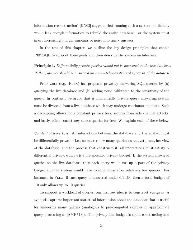
information reconstruction” [DN03] suggests that running such a system indefinitely

would leak enough information to rebuild the entire database – or the system must

inject increasingly larger amounts of noise into query answers.

In the rest of this chapter, we outline the key design principles that enable

PrivSQL to support these goals and then describe the system architecture.

Principle 1. Differentially private queries should not be answered on the live database.

Rather, queries should be answered on a privately-constructed synopsis of the database.

Prior work (e.g. Flex) has proposed privately answering SQL queries by (a)

querying the live database and (b) adding noise calibrated to the sensitivity of the

query. In contrast, we argue that a differentially private query answering system

must be divorced from a live database which may undergo continuous updates. Such

a decoupling allows for a constant privacy loss, secures from side channel attacks,

and lastly, offers consistency across queries for free. We explain each of these below:

Constant Privacy Loss All interactions between the database and the analyst must

be differentially private – i.e., no matter how many queries an analyst poses, her view

of the database, and the process that constructs it, all interactions must satisfy ε-

differential privacy, where ε is a pre-specified privacy budget. If the system answered

queries on the live database, then each query would use up a part of the privacy

budget and the system would have to shut down after relatively few queries. For

instance, in Flex, if each query is answered under 0.1-DP, then a total budget of

1.0 only allows up to 10 queries.

To support a workload of queries, our first key idea is to construct synopses. A

synopsis captures important statistical information about the database that is useful

for answering many queries (analogous to pre-computed samples in approximate

query processing ss [AMP+13]). The privacy loss budget is spent constructing and

24

releasing the synopses. Once released, subsequent queries are answered using only

the synopsis and not the private database. Since the synopsis is public, there is no

privacy cost to querying it and an unlimited number of queries can be answered –

though the fundamental law also implies that some query answers will be poorly

approximated, see Principle 2 for further discussion.

Side Channel Attacks Answering queries on a live database has safety issues – the

observed execution time to answer a query on the live database could break the

differential privacy guarantee and reveal sensitive properties about the records in

the database. For instance, consider a table storing properties of nodes (in a node

table) and edges (in an edge table) in a social network. Suppose the analyst queries

for the number of edges connected to users over the age of 90. Suppose Bob is

the only person in the database with age > 90 and has a thousand friends. With

Bob in the database, the query answer would be 1000. If Bob’s record were not in

the database, the answer to the query is 0. Any differential privacy mechanism for

answering this query would add enough noise to obfuscate this difference. However,

a typical DP mechanism (like Flex) would not hide the time taken to compute

the answer. Without Bob, the live database would identify this query as joining an

empty intermediate table with the edge table, and hence would return quickly. On

the other hand, with Bob in the database, the join may take perceptibly more time,

thus revealing the presence of Bob.

Such timing attacks are avoided if analysts are only exposed to a private synopsis

over the data that is constructed offline. Continuing the above example, the private

synopsis generation may take more or less time depending on whether Bob’s record

is in the database, but this is hidden from the analyst who only interacts with the

private synopsis.

25

Consistency Typical differentially private mechanisms work by adding random noise

to query answers. Therefore, if queries were answered on the live database, an analyst

would see different query answers to the same queries – unless the system cached pre-

vious queries and answers; which is indeed akin to maintaining a synthetic database.

Moreover, relationships between queries may also be distorted. For instance, due to

noise, the total number of males in a dataset could be smaller than the number of

males of age 20-50 (while in the true data the reverse must clearly be true). If one

were answering queries on the live database (like in Flex), the burden of making

noisy answers consistent would be shifted to the analyst.

Since we propose to generate a private synopsis, which is already differentially

private, (a) no further noise needs to be added and (b) we can ensure that the private

synopsis is consistent. A downside of answering queries on a private synopsis is that

updates to the database are not reflected in the query answers. We discuss this in

more detail in Chapter 9.

Principle 2. The private synopsis must be tuned to answer queries for an input

query workload.

Synopses generated for selected views There is considerable prior work on generating

a differentially private statistical summary for a single table. Such strategies have

been shown to support workloads of simple (linear) queries. But if a synopsis were

generated for each base table in the schema, it is known that complex queries, such

as the join of two tables, would be poorly approximated [MPRV].

This motivates the second key idea: to support complex queries, we select a set

of (complex) views over the base tables and then generate a synopsis for each of the

selected views. Our approach is based on the assumed availability of a representative

workload, a set of queries that captures, to a first approximation, the kinds of queries

that users are likely to ask in the future. Views are selected so that each query in

26

the representative workload can be answered with a linear query on a single view.

Intuitively, views encode the join structures that are common in the workload.

The celebrated result by Dinur-Nissim [DN03], the Fundamental Law of Infor-

mation Reconstruction, shows that a database containing n bits can be accurately

reconstructed by an adversary that submits n log2 n counting queries, even if each of

the queries has o(√n) additive noise. This implies that we cannot hope to accurately

answer too large a set of queries from any single synopsis under strong privacy guar-

antees. It therefore means that we must specify as input a representative workload

of queries to be answered. This workload can be either a list of explicitly defined

queries, or a set of parameterized queries – where constants are replaced by wild-

cards. The private synopsis will be designed to provide answers to the representative

workload with high accuracy. Of course, if the workload contains too many queries

then we can not answer all of them with high accuracy without violating the Funda-

mental Law of Reconstruction. Thus our accuracy guarantees on the queries in the

representative workload are best-effort. Our system also tries to answer queries that

are not in the input workload and if it can’t, then it informs the user.

Principle 3. Private synopses may need to be generated over views defined on the

base tables and not just on the base tables.

Prior work has shown that queries involving the join of two tables cannot be

answered accurately just using private synopses that have been generated indepen-

dently from each of the tables. For instance, Mironov et al. [MPRV] show a Ω(√n)

lower bound on the error of computing the intersection between two tables given

differentially private access to the individual tables (and not their join). The intu-

ition behind this result follows from the definition of differential privacy. Since join

keys are typically unique, no differentially private algorithm can preserve the key.

Thus, joins have to be done on coarser quasi-identifiers which are associated with a

27

sufficiently large number of tuples.

In contrast, given access to a view that encodes the join over the two base tables,

computing the size of the join is a counting query that can be answered with constant

error. Thus, if one expects to receive many queries involving the join between two

tables, the system must generate private synopses from an appropriate view over the

base tables and not just from the base tables themselves.

Principle 4. View sensitivity must be bounded and tractable.

View sensitivity bounded using rules and truncation: When PrivSQL generates a syn-

opsis for each view, it ensures the synopsis generator is differentially private with

respect to its input, a view instance. A subtle but important point is that achieving

ε-differential privacy with respect to a view does not imply ε-differential privacy with

respect to the base relations from which the view is derived. This is because a single

change in a base relation could affect multiple records in the view. For example,

imagine a view that describes individuals living in households along with employ-

ment characteristics of the head of household. Changing the employment status of

the head of an arbitrary household would affect the records of all members of that

household. To correctly apply differential privacy, we must know (or bound) the view

sensitivity, which is informally defined as the worst-case change in the view due to

the insertion/deletion of a single tuple in a base relation.

This brings us to the third key idea: we introduce novel techniques for calculat-

ing a bound on view sensitivity. Exact sensitivity calculation is hard, even unde-

cidable [AFG16]. We employ a rule-based calculator to each relational operator in

the view definition (which is expressed as a relational algebra expression). The per

operator bounds compose into an upper bound on the global sensitivity of the view.

An additional challenge is that some queries have high, even unbounded, sensi-

tivity because of worst case inputs. The previous example has a sensitivity that is

28

equal to the size of the largest possible household. Our approach to addressing high

sensitivity queries is to use truncation to drop records that cause high sensitivity

(e.g., large households). By lowering sensitivity, truncation lowers the variance in

query answers at the expense of introducing bias that arises from data deletion. We

describe techniques for using the data to privately estimate the truncation threshold

and we empirically explore the bias-variance trade-off.

Principle 5. Sensitivity estimation should be policy agnostic.

Privacy at multiple resolutions: A key design goal of PrivSQL is to allow data owners

to select the privacy policy that is most appropriate to their particular context.

Differential privacy, as formally defined, assumes the private data is encapsulated

within a single relation. Adapting it to multi-relational data is non-trivial, especially

given integrity constraints like foreign key constraints. When a tuple is removed from

one relation, it can cause (cascading) deletions in other relations that are linked to

it through foreign keys.

Our fourth key idea is extending differential privacy to the multi-relational set-

ting. With our approach, one relation is designated as the primary private relation,

but the privacy protection extends to other secondary private relations that refer to

the primary one through foreign keys. We show this allows the data owner to vary

the privacy resolution (e.g., to choose between protecting an individual vs. an entire

household and all its members). We describe this extension in Section 3.2 and relate

it to prior literature.

View rewriting allows policy flexibility: The challenge with supporting flexible privacy

policies is that now view sensitivity will depend on the policy. For example, a policy

that protects entire households would generally have higher sensitivity than a policy

that protects individuals. PrivSQL is designed to offer the data owner flexibility

29

q

ỹ

Analyst

Query Answering Phase

CᴏᴍᴘᴜᴛᴇQᴜᴇʀʏ

MᴀᴘQᴜᴇʀʏ

Private Synopsis Generation Phase

Data Owner Q, R, ε

Private Synopses

VRᴇᴡ

ʀɪᴛᴇ

Sᴇɴs

Cᴀʟ

ᴄ

Bᴜᴅ

ɢᴇᴛA

ʟʟᴏᴄ

Pʀɪᴠ

SʏɴG

ᴇɴ

VSᴇʟᴇᴄᴛᴏʀGenerate views based on Q

V1

V2

Vn

Figure 4.1: Architecture of the PrivSQL System

to choose the appropriate policy and the system will automatically calculate the

appropriate sensitivity.

The fifth and final key idea is that we use view rewriting to ensure correct, policy-

specific sensitivity bounds. Rewriting makes explicit whether a view depends on the

primary private relation, even in cases when the view does not mention it! After

rewriting, downstream components (such as sensitivity calculation and synopsis gen-

eration) can be oblivious to the particular policy and apply conventional differential

privacy on the primary private relation.

4.2 System Architecture

We now review the architecture of PrivSQL (illustrated in Fig. 4.1) and the algo-

rithms of the two main operational phases. The first phase is the synopsis generation

phase where a representative workload is used to guide the selection of views followed

by the differentially private construction and publication of a synopsis for each of

the selected views. Next is query answering phase where each user query is mapped

to the appropriate view and then answered using the released synopsis of that view.

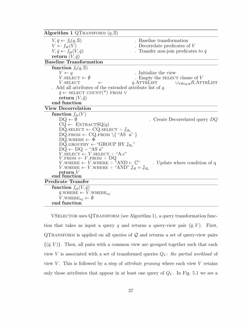
Synopsis generation phase As described in Algorithm 1, this phase takes as input

a database instanceD, which is private, and its schema S, which is considered public.

It also takes a representative query workload of SQL queries, Q, and a privacy policy

30

Algorithm 1 Synopsis-GenerationRequire: Schema S, database D, representative workload Q, privacy policy P = (R, ε).Ensure: A set of views V and private synopses SV V ∈V1: V ← VSelector(S,Q) . Choose views based on workload2: Reserve εmf to estimate thresholds for relations in views.3: ε← ε− εmf4: for each view V in V do5: V τ, ← VRewriter(V, P, S)6: τV ← Estimate truncation thresholds using εmf/|V|7: ∆V ← SensCalc(V τ,, S, τV )8: QV ← q | q ∈ Q ∧QTransform(q,S) = (q, V )9: end for

10: for each V ∈ V do11: εV ← BudgetAlloc(V, [QV ], [∆V ], ε)

12: SV ← PrivSynGen(V τ,, V τ,(D), εV , QV )13: end for14: return (V, SV ) for each V ∈ V

Algorithm 2 Query-Answering

Require: Query q, schema S, views V, synopses S.Ensure: Query answer or ⊥1: (q, V )← QTransform(q,S)2: if V ∈ V then3: return ComputeQueryAnswer(q, SV )4: else5: return ⊥6: end if

P = (R, ε) that specifies a privacy budget ε and a primary private relation R (formally

defined in Section 3.2).

First, the VSelector module (line 1) uses the representative workload Q to

select a set of view definitions V .

Next, each view (interpreted as a relational algebra expression) is rewritten using

the VRewriter module (line 5) in two ways. First, truncation operators are in-

cluded when there is a join on at attribute that may result in a potentially unbounded

number of output tuples. The truncation operator enforces a bound on join size by

throwing away join keys with a multiplicity greater than a threshold. The thresholds

can be learnt from the data (line 6) in a differentially private manner. Next, base

tables in the view definition are rewritten using semijoin expressions, which makes

explicit the foreign key dependencies between the primary private relation and other

31

base tables. This ensure that the computed sensitivity matches the privacy policy.

Next, the SensCalc module (line 7) computes for each rewritten view V , an

upper bound on the global (or worst case) sensitivity ∆R(V ). The sensitivity bound

∆V is used in the privacy analysis and affects how much privacy loss budget is

allocated to each view.

Synopsis generation for each view is guided by a partial workload QV , which is

the set of queries from the representative workload Q the can be answered by this

view. The set QV is constructed (line 8) by applying the function QTransform

(constructed by VSelector) to each query in Q. This function transforms a query

q into a pair (q, V ) where q is a new query that is linear (or a simple aggregation

without involving joins) on view V .

Lastly, and for each view V we generate a private synopsis. Each synopsis is

allocated a portion of the total privacy loss budget. The BudgetAlloc component

(line 11) determines the allocation based on factors like view sensitivity and/or the

size of QV . Finally, the PrivSynGen component takes as input the view definition,

view instance V (D), a set of linear queries QV , and a privacy budget εV and returns

a differentially private private synopsis SV . This module runs an εV -differentially

private algorithm and outputs either a set of sythetic tuples or a set of query answers

– like histograms or a set of counts.

We present our generalization of differential privacy for relational databases in

Section 3.2. We outline VSelector in Section 5.1. We describe SensCalc and the

truncation rewrite in Section 5.2, and the semijoin rewrites in Section 5.3. PrivSyn-

Gen and BudgetAlloc are described in Sections 5.4 and 5.5 respectively. Lastly,

the privacy proof of PrivSQL is presented in Section 5.6

Query answering using views is a well studied problem [Hal01] and in PrivSQL

is performed by the query answering phase. More specifically, it uses the function

32

QTransform, described above, to convert q into a query q that is linear on a view

V . If V is one of the views for which PrivSQL generated a synopsis, then q is then

executed on the appropriate private synopsis to produce an answer. If the query

cannot be mapped to any view, it returns ⊥. As our techniques for query answering

are straightforward, we omit further details.

End-to-End Privacy Executing an εV -DP algorithm on V (D) can be shown to satisfy

∆V εV -DP over the base tables [McS09b].

The overall privacy of PrivSQL follows from the sequential composition property

of differential privacy [DR14]. As long as the budget allocation satisfies:∑V ∈V

∆V εV ≤ ε− εmf (4.1)

where εmf is the budget allocated to learning truncation thresholds, then, PrivSQL

always satisfies the policy-specific privacy guarantee with privacy loss of ε (see Sec-

tion 5.6). Note that query answering has no privacy cost.

33

5

Generating Private Synopses Based on Views

5.1 View Selection

View selection in PrivSQL is performed by the VSelector module, which takes as

input a set of representative queries Q over the schema S and returns (V ,QTransform).

V is a set of views such that all queries of Q are linearly answerable using some view

V ∈ V . QTransform is an internal function of VSelector that transforms

queries of Q and helps generate the set of views V . Our system exposes QTrans-

form outside VSelector so that other components of PrivSQL can map new

queries to the set of views V .

Definition 5.1.1. A query q over schema S is answerable using a view V if there

is a query q defined on the attributes in V such that for all database instances D ∈

dom(S), we have, q(D) = q(V (D)). Additionally, we say that q is linearly answerable

using V , if q is linear on V .

Linear answerability ensures that queries in Q can be directly answered from

some V ∈ V without additional join or group-by operations. Moreover, the privacy

analysis of sets of linear queries is easy and it allows the use of well known workload-

34

V1: SELECT age, race FROM Person;

q1: SELECT count(*) FROM V1 WHERE V1.age < 18;q2: SELECT count(*) FROM V1 WHERE V1.race = ‘Asian’ AND V2.age >= 21;

V2: SELECT relp, race, cnt FROM Person P, (SELECT count(*) AS cnt, hid FROM Person GROUP BY hid) AS P2 WHERE P2.hid = P.hid;q3: SELECT count(*) FROM V2 WHERE V2.cnt = 2;q4: SELECT count(*) FROM V2 WHERE V2.race = Asian AND V2.cnt = 3;

VSᴇʟ

ᴇᴄᴛᴏ

ʀq1: SELECT count(*) FROM Person WHERE age < 18;q2: SELECT count(*) FROM Person WHERE race = ‘Asian’ AND V2.age >= 21;q3: SELECT count(*) FROM Person p WHERE (select count(*) from Person p1 where p1.hid = p.hid) = 2;q4: SELECT count(*) FROM Person p WHERE (SELECT count(*) FROM Person p1 WHERE p1.hid = p.hid) = 3 and p.race = white and p.relp = 0;

Rep

rese

ntat

ive

Wor

kloa

dq

1, q

2, q

3, q

4

Figure 5.1: An execution of VSelector on a workload of 4 queries,producing two distinct views.

aware algorithms in the PrivSynGen module, as well as other optimizations like

workload driven domain reductions.

In Fig. 5.1 we show an execution of VSelector on workload Q = q1, q2, q3, q4,

for which VSelector produces two distinct views V1 and V2, under which all queries

ofQ are linearly answerable. More specifically, q1 and q2 can be answered using linear

queries q1 and q2 on V1. Similarly, q3 and q4 can be answered using linear queries q3

and q4 on V2. For the remainder we denote the transformed workloads QV1 = q1, q2

and QV2 = q3, q4 as the partial workloads of views V1 and V2 respectively.

5.1.1 Design Considerations:

The goal of VSelector is to produce views such that (a) all queries of Q can be

answered from a view and (b) the total privacy loss of PrivSQL as expressed in

Eq. (5.8) is minimized.

An initial approach to minimize the privacy loss is to release a single view Vone.

Let VSelectorone denote this approach, with Vone the universal view constructed

35

by joining all relations under key-foreign key constraints. 1 It is clear that under

Vone all queries of Q are answerable. However, VSelectorone does not guarantee

linear answerability – see q3 and q4 of Fig. 5.1 that are not linearly answerable using

Vone, as they require self joins on the Person relation. In addition, VSelectorone

does not necessarily minimize the privacy loss of Eq. (5.8) since the factor ∆Vone will

be as large as the largest sensitivity of a query answered from Vone. This penalizes

low sensitivity queries, as they will be answered by the high sensitivity view Vone.

Another way to minimize the privacy loss is to generate views with a small ∆V

value. This can be achieved from VSelectorall, that for each query q ∈ Q returns a

view Vq containing all tuples that q accesses. Evidently, VSelectorall satisfies linear

answerability for all queries of Q, since a query q is linearly answerable by the simple

linear query q = select count(*) from vq;. Moreover, all views Vq returned

from VSelectorall have the smallest possible ∆Vq . Still, VSelectorall does not

minimize the privacy loss, as it fails to take advantage of parallel composition [DR14]

between queries of Q. For instance, consider queries q1 and q2 from Fig. 5.1 that have

no overlap – as q1 counts underage people, and q2 counts heads of households over

21 years old. For these queries, VSelectorall will create views V1 and V2, resulting

in synopses SV1 and SV2 generated with privacy budgets εV1 and εV2 s.t. ε = εV1 + εV2 .

However, both queries could be answered from a single synopsis SV generated with

a total privacy budget of ε, resulting in higher accuracy answers.

5.1.2 Approach

We propose a heuristic algorithm VSelector that: (a) satisfies linear answerability

w.r.t. Q, (b) each partial workload QV contains a non-trivial number of queries for

efficient query sensitivity analysis, (c) each QV is sensitivity homogeneous, and (d)

returned views have low complexity for tractable sensitivity analysis.1 If the schema is not semijoin-reduced, then joining all relations using the foreign keys does not capture all rows

of all base tables. We ignore this detail since we do not use the universal relation approach to view selection.

36

Algorithm 1 QTransform (q,S)

V, q ← fb(q,S) . Baseline transformationV ← fdc(V ) . Decorrelate predicates of VV, q ← fpt(V, q) . Transfer non-join predicates to qreturn (V, q)

Baseline Transformationfunction fb(q,S)

V ← q . Initialize the viewV .select ← ∅ . Empty the select clause of VV .select ← q.AttrList ∪∀R∈q.onR.AttrList

. Add all attributes of the extended attribute list of q.q ← select count(*) from vreturn (V, q)

end functionView Decorrelation

function fdc(V )DQ ← ∅ . Create Decorrelated query DQCQ ← ExtractSQ(q)DQ.select ← CQ.select + JRc

DQ.from ← CQ.from \ “AS a” DQ.where ← ΦDQ.groupby ← “GROUP BY JRc”DQ ← DQ + “AS a”V .select ← V .select + “A.c”V .from ← V .from + DQV .where ← V .where + “AND c C” . Update where condition of qV .where ← V .where + “AND” JR = JRc

return Vend function

Predicate Transferfunction fpt(V, q)

q.where ← V .wherenjV .wherenj ← ∅

end function

VSelector uses QTransform (see Algorithm 1), a query transformation func-

tion that takes as input a query q and returns a query-view pair (q, V ). First,

QTransform is applied on all queries of Q and returns a set of query-view pairs

(q, V ). Then, all pairs with a common view are grouped together such that each

view V is associated with a set of transformed queries QV : the partial workload of

view V . This is followed by a step of attribute pruning where each view V retains

only those attributes that appear in at least one query of QV . In Fig. 5.1 we see a

37

full execution of our VSelector on a workload of 4 queries, resulting in views V1

and V2 with partial workloads QV1 = q1, q2 and QV2 = q3, q4 respectively.

QTransform is fully described in Algorithm 1, on a high level its functionality

is summarized from 3 sequential steps: (a) the baseline query transformation fb,

(b) the view decorrelation step fdc, and (c) the predicate transfer step fpt, each

described in Algorithm 1. More specifically, the baseline transformation fb creates a

simple view V that (a) contains all tuples that the input query accesses q and (b)

ensures that the view has all attributes accessed from the query. Next, the function

fdc performs decorrelation [BMSU86] on a view V by rewriting correlated subqueries

of the view in terms of joins. Finally, fpt operates on input (q, V ) and moves all

filtering operations from the view V to the query q.

In the example of Fig. 5.1 we can see how QTransform operates on query q3

which contains a correlated subquery in its where clause.

which contains a correlated sub-query is transformed to the pair (V2, q3).

5.2 View Sensitivity Analysis

Computing the global sensitivity of a SQL view (lines 6-7 of Algorithm 1) is a hard

problem [AFG16], as single changes in a base relation could affect a large (or even

unbounded) number of records in the view. Moreover, complex privacy policies

resulting in secondary private relations (see Definition 3.2.2), further complicate

sensitivity estimation.

In this section we focus on simple privacy policies resulting only in a primary pri-

vate relation in the schema and discuss complex policies in Section 5.3. Section 5.2.1

describes SensCalc a rule-based algorithm that computes the constraint-oblivious

down sensitivity of a view V on a database instance D. Section 5.2.2 describes how

to rewrite a view using truncation operators so that for simple privacy policies, the

sensitivity output by SensCalc is indeed the global sensitivity of the rewritten view

38

Table 5.1: Update rules for sensitivity and max-frequency bounds. Newrules are shaded.

Operators Sensitivity Bound∆R(S)

S = πA(R) ∆R(R)

S = σφ(R) ∆R(R)

S = γA(R) ∆R(R)

S = γCOUNTA (R) 2∆R(R)

S = R1 ./A1=A2 R2 orS = R1 nA1=A2R2

where A1,A2 are from S

General casemf(A1, R1) · ∆R(R2)+

mf(A2, R2) · ∆R(R1)+

∆R(R1) · ∆R(R2)

No common max(mf(A1, R1) · ∆R(R2),ancestors mf(A2, R2) · ∆R(R1))

Join on key mf(A2, R2) · ∆R(R1)+

(A1 ∈ Keys(R1)) ∆R(R2)

S = τA,k(R) k · ∆R(R)

Operators Max Frequency Bound Key Setmf(A′, S),A′ ⊆ attr(S) Keys(S)

S = πA(R) mf(A′, R) A′ ⊆ attr(S) | A′ ∈ Keys(R)S = σφ(R) mf(A′, R) A′ ⊆ attr(S) | A′ ∈ Keys(R)S = γA(R) mf(A′, R) A ∪ A′ ⊆ attr(S) | A′ ∈ Keys(R)

S = γCOUNTA (R) mf(A′, R) A ∪ A′ ⊆ attr(S) | A′ ∈ Keys(R)S = R1 ./A1=A2 R2 orS = R1 nA1=A2R2

where A1,A2 are from S

max(mf(A2, R1) · mf(A2, R1),mf(A1, R2) · mf(A1, R2))

where Ai = A′ − attr(Ri)A′ ∈ Keys(R2)|A1 ∈ Keys(R1)∪A′ ∈ Keys(R1)|A2 ∈ Keys(R2)

S = τA,k(R) min k, mf(A′, R) if A ⊆ A′; A′ ⊆ S|A′ ∈ Keys(R)

V τ (see Theorem 5.2.1). Section 5.2.3 presents a DP method for learning thresholds

needed for truncation operators.

We assume w.l.o.g. that a view V is expressed in relational algebra. This expres-

sion can be viewed as a tree, where internal nodes are algebra operators and the leaf

nodes are base relations of S. First, we propose SensCalc a rule-based algorithm

for computing a bound on the sensitivity of a view (Section 5.2.1). We also bound

the sensitivity of join operations by a query rewrite – by adding targeted truncation

operators on the query plan of a view (Section 5.2.2). Our main theoretical result

of this section, Theorem 5.2.1, shows that any view V can be rewritten to a view V ′

such that the sensitivity calculator returns a bound on the global sensitivity of V ′.

39

In the sequel (Section 5.3) we use our results to extend PrivSQL so that it can

automatically handle complex privacy policies.

5.2.1 Sensitivity Calculator

Sensitivity estimation in PrivSQL is performed by the SensCalc module. This

module computes the constraint-oblivious down sensitivity, a sensitivity variant that

captures the maximum change caused by removing any one tuple from the primary

private relation R.

Definition 5.2.1 (Constraint-Oblivious Down Sensitivity). Given schema S and a

privacy policy (R, ε), the constraint-oblivious down sensitivity of V given D w.r.t. R,

denoted by ∆R(V,D), is defined as the maximum number of rows that change in V

when removing a row from R.

∆R(V,D) = maxr∈dom(R)

V (D)4V (D− r), (5.1)

where D− r means removing tuple r from instance D.

In the case of simple privacy policies, the constraint-oblivious down sensitivity

is equivalent to the down sensitivity (defined in Section 3.2 Eq. (5.2)), i.e., for any

simple policy P and any V : ∆R(V,D) = ∆CR(V,D). Combined with truncation

rewrites described later, the sensitivity output by SensCalc will be the right global

sensitivity for simple policies.

SensCalc is a recursive rule-based sensitivity calculator that takes as input V ,

schema S, and a relation R designated as the primary private relation. It also has

access to mf, a function that provides bounds on the maximum frequency mf of any

attribute combination of the base relations in V . The final result is ∆R(V, mf), as it

depends on the bounds supplied from mf – when clear from context we write ∆R(V ).

Given an input view V and mf, the sensitivity calculator computes ∆R(V, mf)

by a recursive application of the rules in Table 5.1 to each subexpression S of V .

40

⨝hid

πrelp, race, cnt

γhid

Person

Trunchid,k

Person

⨝hid

πrelp, race, cnt

Person

Persons

γhid

Trunchid,k

⨝hid

⋉hid

Household

Person

Trunchid,k

⋉hid

Household

γhid

πrelp, race, cnt

Δ=1, mf(hid)=1Δ=0, mf(hid)=k

Δ=k, mf(hid)=k

Δ=0, mf(hid)=F

Δ=1, mf(hid)=1

Δ=0, mf(hid)=k

Δ=k, mf(hid)=k

Δ=2k,IsKey(hid)

Δ＝2k^2+k

Primary Private Relation

Secondary Private Relation

PersonΔ=0,

mf(hid)=F

Query Plan Truncation Rewrite

Figure 5.2: Truncation rewrite operation (Alg 2)

The bounds at the base relations are as follows: the sensitivity bounds ∆R(R) =

1 and ∆R(R) = 0 for R ∈ S − R and the max-frequency bounds are supplied

by mf. In Table 5.1 we summarize the rules of SensCalc. Operators such as

project, select, and groupby do not increase the sensitivity bound of their

input relation, while groupby-count doubles it. equijoin results in relations

with higher sensitivity bounds compared to its inputs. In terms of the mf bounds,

most unary operators shown in Table 5.1 have unchanged mf. Note that we restrict

the equijoin operator to join on attributes from the base relations in S. The last

row refers to a truncation operator, which is described in Section 5.2.2.

These rules are similar to those of elastic sensitivity [JNS18], but with some key

differences that allow for a tighter sensitivity analysis. SensCalc uses additional

rules using keys, as shown in the last column of Table 5.1. The new rules keep

track of key constraints through operators. This allows the addition of new rules for

joins on key attributes that permit lower sensitivity bounds than a standard join, as

illustrated in the following example.

Example 2 (Sensitivity Calculation). Consider calculating the sensitivity of V2 from

Fig. 5.1 under Person policy. A relational algebra expression for view V2 is (Fig. 5.2

41

(left))

πrace,relp,cnt(Person ./hid (γCOUNThid (Person))).

V2 has a row for each person reporting the person’s race, relp, and size of their

household. SensCalc initializes ∆R(Person) to 1 and applies the rules of Table 5.1

bottom up. First the groupby-count operator is processed, resulting in S =

γCOUNThid (Person) with ∆R(S) = 2 · ∆R(Person) = 2 and S has hid as a key. Next, the

equijoin operator is processed, joining on key hid of S, producing S./ = Person ./hid

S with: ∆R(S./) = F · ∆R(S) + ∆R(Person) = F · 2 + 1 where F = mf(hid,Person).

Note that without the “Join on key” rule, the bound would be (F · 3 + 2). This differ-

ence is only exacerbated for views with more joins. Last, the projection operator

is processed, leaving the bound unchanged.

Given D, V and upper bounds on max-frequency mf, we can show that ∆R(V, mf)

calculated by SensCalc is an upper bound on ∆R(V,D), and thus an upper bound

on the down sensitivity ∆CR(V,D) for simple policies.

5.2.2 Bounding Sensitivity via Truncations

As shown in Example 2, the sensitivity bounds produced by the SensCalc can be

dependent on the max-frequency bounds on base relations. We now show how to

add truncation operators to the view expression. These operators delete tuples that

contain an attribute combination appearing in a join and whose frequency exceeds

a truncation threshold k specified in the operator. The sensitivity will no longer

depend on max-frequencies but rather on the thresholds. If thresholds are set in a

data-independent manner or using a DP algorithm, then we show that the sensitivity

computed by SensCalc is indeed a bound of the global sensitivity.

Definition 5.2.2 (Truncation Operator). The truncation operator τA,k(R) takes in a

relation R, a set of attributes A ⊆ attr(R) and a threshold k and for all a ∈ dom(A),

42

Algorithm 2 Truncation Rewrite (V, R,k)

1: Initialize V τ ← V2: for every path pl from leaf relation Rl to root in V do3: for every R1 ./A1=A2 R2 on pl, where A1 ⊆ attr(Rl) do4: .(semijoin is also treated as a special equijoin)5: if A1 /∈ Keys(R1) and R is a base relation of R2 then6: k ← kA1

7: Insert τA1,k(Rl) above Rl in V τ

8: A ← A∪ (A1)9: end if

10: end for11: end for12: Return V τ

if f(a,A, R) > k, then any r from R with r[A] = a is removed.

Truncation rewrite (see Algorithm 2) adds truncation operators to V and forms

a new query plan V τ . The algorithm takes as input a view V , a primary private

relation R, and a vector of truncation thresholds k, indexed by the attribute subset

to which the threshold applies. It traverses every path pl from relation Rl to the root

operator and every join R1 ./A1=A2 R2 on this path. If one of the join attributes is

from Rl—say A1 ⊆ Rl—and A1 is not a key for R1 and the primary private table R

appears as a base relation in the expression R2, then we insert τA1,k(Rl) above Rl in

V τ . The rules of SensCalc for the truncation operator can be found on Table 5.1.

In terms of the maximum frequency bound, it is at most k for any A′ ⊇ A.

Example 3. Fig. 5.2 (right) shows the truncation operators are inserted before Per-

son relation. The truncation operators cut down the maximum frequency of hid

to k so that the sensitivity bound can be bounded by 3k, even when mf for house-

hold id in Person is unbounded. In this case, ∆R(S./) = k · ∆R(γCOUNThid (Person)) +

∆R(τhid,k(Person)) = k · 2 + k = 3k.

After truncation rewrite is applied, the estimated sensitivity no longer depends

on mf, but rather on the truncation thresholds. If the thresholds are set in a data

independent manner, or using a DP algorithm (as discussed in Section 5.2.3) we can

43

show that the sensitivity output by SensCalc on V τ is the global sensitivity for

simple policies.

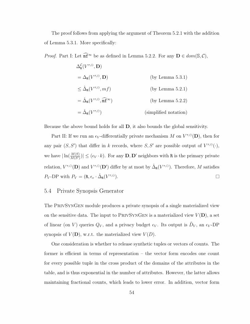
Theorem 5.2.1. Consider a schema S = (R1, . . . , Rk) with foreign constraints C,

and simple privacy policy (R, ε). For any V , let V τ denote the truncation rewrite of

V using a fixed set of truncation thresholds k (Algorithm 2). The global sensitivity

of V τ is bounded by SensCalc:

∆CR(V τ ) = ∆R(Vτ ) ≤ ∆R(V

τ ).

Let M be εv-differentially private algorithm that runs on V τ (D). Then M satisfies

PV -DP with PV = (R, εv · ∆R(Vτ )).

Proof. Part I: Let mf∞ denote unbounded max frequencies: mf∞(A, R) = ∞ for all

A ⊆ attr(R) and for all R ∈ S.

For any D ∈ dom(S, C),

∆CR(V τ ,D)

= ∆R(Vτ ,D) For simple policies

≤ ∆R(Vτ ,mf) (by Lemma 5.2.1)

= ∆R(Vτ , mf∞) (by Lemma 5.2.2)

= ∆R(Vτ ) (simplified notation)

Because the above bound holds for all D it also bounds the global sensitivity.

Part II: If we run an εV -differentially private mechanism M on V τ (D), then for

any pair (S, S ′) that differ in k records, where S, S ′ are possible output of V τ (·), we

have | ln( M(S)M(S′)

)| ≤ (εV · k). For any D,D′ neighbors with R is the primary private

relation, V τ (D) and V τ (D′) differ by at most by ∆R(Vτ ). Therefore, M satisfies

PV -DP with PV = (R, εv · ∆R(Vτ ).

44

The truncation rewrite introduces bias: i.e., ∃D, V (D) 6= V τ (D). However, the

global sensitivity computed after truncation is usually much smaller reducing error

due to noise. We empirically measure the effect of truncation bias in Section 7.1.4.

Our truncation methods are related to Lipschitz extension techniques which also

tradeoff bias for noise typically by truncating the data. Existing methods apply to

specific queries on graphs [HLMJ09, KRSY11, KNRS13, DLL16, DZBJ18] or only

on monotone queries [CZ13]. Our technique applies to general relational data and

more complex queries.

To proof of Theorem 5.2.1 is supported by the following two lemmas that show

given a view V , SensCalc calculates a upper bound on the constraint-oblivious

down sensitivity of V on input D.

Lemma 5.2.1. Consider an acyclic schema S = (R1, . . . , Rk) with foreign con-

straints C, a single private relation R ∈ S, and no secondary private relations. For

all views V , inputs D, base tables S, and all A ⊆ attr(S), if mf(A, S) ≤ mf(A, S)

then: ∆R(V,D) ≤ ∆R(V, mf).

Proof. The rules presented in Table 5.1 with white background are first proposed in

[JNS18]. The new rule on joining on a key attribute is as follows. Let S = R1 ./A1=A2

R2 an equijoin where A1 is a key attribute on R1. The removal of a single tuple can

affect mf(A2, R2)mf(R1) tuples in S from the influence of R1. However, A1 is a key

on R1 with max frequency 1, that means that the influence of R2 is mf(R2). Hence

the overall sensitivity of S is bounded by mf(A2, R2)mf(R1) + mf(R2).

The new rule on the proposed truncation operator is as follows. Let S = τA,k(R)

a truncation on relation R for attribute A, at value k. This means that S will contain

tuples with value for A at most k. Let R′ a neighboring instance: R′ = R−t, s.t.

v = t.A has multiplicity k + 1, and S ′ = τA,k(R′). It is then obvious that S ′ has k

less tuples than S since truncation in R does not affect k tuples with value v. Hence

45

Algorithm 3 LearnThreshold (D, V τ , θ, εmf )

1: Traverse operators in V τ from leaf to root and add each truncation operator toT if it is not in the list.

2: for τA,k(R) ∈ T do3: q′i ← sub-tree at τA,k(R) ∈ V τ . Truncate at k = i4: Q← (|q′i|−|R|·θ)

i| i = 1, 2, . . .

5: Set i← SVT(D, Q, 0, εmf/|T |) as the truncation threshold for τA,k(R)6: end for

the sensitivity of τA,k(R) is mf(R)k.

We show in Lemma 5.2.2 that truncation eliminates the need for tight bounds on

max frequencies.

Lemma 5.2.2. For any V , let V τ denote the truncation rewrite of V using a fixed set

of truncation thresholds k. Let mf∞ denote unbounded max frequencies: mf∞(A, R) =

∞ for all A ⊆ attr(R) and for all R ∈ S. For any mf such that mf(A, S) ≤ mf(A, S)

for all base relations S of V and all A ⊆ attr(S): ∆R(Vτ , mf) = ∆R(V

τ , mf∞)

Proof. Algorithm 2 adds truncation operators on top of base relations that partici-

pate in joins (later in the tree of V ). Since SensCalc works in a bottom-up fashion,

this removes the dependency of SensCalc on the true max frequencies of the base

tables. Thus, ∆R(Vτ , mf) = ∆R(V

τ , mf∞).

Hence, the global sensitivity of the rewritten query ∆CR(V τ ) is upper bounded by

∆R(Vτ ) outputted by SensCalc.

5.2.3 Learning Truncation Thresholds

In Section 5.2.2 we described how we use truncation operators to bound the computed

view sensitivity. From Definition 5.2.2 we observe that the threshold k plays a crucial

role in the function of the truncation operators.

Setting this threshold can be done independently of the underlying data (e.g.,

based on public knowledge), or in a privacy-preserving, data dependent fashion. We

46

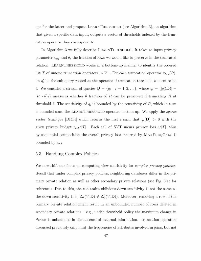
opt for the latter and propose LearnThreshold (see Algorithm 3), an algorithm

that given a specific data input, outputs a vector of thresholds indexed by the trun-

cation operator they correspond to.

In Algorithm 3 we fully describe LearnThreshold. It takes as input privacy

parameter εmf and θ, the fraction of rows we would like to preserve in the truncated

relation. LearnThreshold works in a bottom-up manner to identify the ordered

list T of unique truncation operators in V τ . For each truncation operator τA,k(R),

let q′i be the sub-query rooted at the operator if truncation threshold k is set to be

i. We consider a stream of queries Q = qi | i = 1, 2, . . ., where qi = (|q′i(D)| −

|R| · θ)/i measures whether θ fraction of R can be preserved if truncating R at

threshold i. The sensitivity of qi is bounded by the sensitivity of R, which in turn

is bounded since the LearnThreshold operates bottom-up. We apply the sparse

vector technique [DR14] which returns the first i such that qi(D) > 0 with the

given privacy budget εmf/|T |. Each call of SVT incurs privacy loss ε/|T |, thus

by sequential composition the overall privacy loss incurred by MaxFreqCalc is

bounded by εmf .

5.3 Handling Complex Policies

We now shift our focus on computing view sensitivity for complex privacy policies.

Recall that under complex privacy policies, neighboring databases differ in the pri-

mary private relation as well as other secondary private relations (see Fig. 3.1c for

reference). Due to this, the constraint oblivious down sensitivity is not the same as

the down sensitivity (i.e., ∆R(V,D) 6= ∆CR(V,D)). Moreover, removing a row in the

primary private relation might result in an unbounded number of rows deleted in

secondary private relations – e.g., under Household policy the maximum change in

Person is unbounded in the absence of external information. Truncation operators

discussed previously only limit the frequencies of attributes involved in joins, but not

47

the change in secondary private relations.

We first present the semijoin rewrite that transforms view V into V so that

the sensitivity computed by SensCalc on V equals its down sensitivity (i.e.,

∆R(V,D) = ∆CR(V ,D)). For example, consider the view V1 from Fig. 5.1 un-

der Household policy where Person is a secondary private relation. In that example,

removing a tuple from Household will result in removing multiple tuples from Person,

thus affecting the sensitivity of V1.

To address these challenges, we introduce the notion of transitive referral and

deletions, which allows reasoning about neighboring databases. We also propose

an additional view rewriting operation, such that even for complex privacy policies

executing the sensitivity calculation algorithm of Section 5.2.1 on the rewritten view

automatically computes the correct sensitivity bounds of the original view.

Transitive Referral and Deletion: If S.Afk → R.Apk is a foreign key constraint,

deleting a row r in relation R results in the cascading deletion of all rows s ∈ S such

that s[Afk] = r[Apk]. Furthermore, if T.A′fk → S.A′pk, then the deletion of record

s ∈ S can recursively result in the deletion of records in T . We define this property

as transitive referral.

Definition 5.3.1 (Transitive Referral). A relation S transitively refers to a relation

R through foreign keys if there exists a relation T such that S.A→ T.B and T tran-

sitively refers to relation R through foreign keys. Moreover, a row s ∈ S transitively

refers to a row r ∈ R if there is a row t ∈ T such that s→ t and t transitively refers

to r. If s transitively refers to r, we denote that s r.

A schema is acyclic if no relation in it transitively refers to itself. We now propose

a method of deriving neighboring databases under acyclic schemas.

Theorem 5.3.1 (Transitive Deletion). Given an acyclic schema S = (R1, . . . , Rk)

with foreign key constraints C, and a privacy policy (Ri, ε). For D ∈ dom(S, C) and

48

r ∈ Di, we denote C(D, (r, Ri)) = (D1 , D2 , . . . , D

k ), where Dj = Dj − t|t ∈

Dj, t r. Then we have:

C(D, Ri) = ∪r∈DiC (D, (r, Ri)).

Proof. First, we show that for all r ∈ Di, C(D, (r, Ri)) ∈ C(D, Ri). As r ∈ Di

and Di = Di − r, we have r /∈ Di . For any Rj and for all Rp that is referred

by Rj: Dj nDp = Dj . Let the following definitions:−→X (Dj, r) = t ∈ Dj|t r,

−→X (Dj, Dp, r) = t ∈ Dj|∃s ∈ Dp, t→ s ∧ s r. Then, we have:

Dj nDp = (Dj −−→X (Dj, r)) n (Dp −

−→X (Dp, r))

= Dj −−→X (Dj, r)−

−→X (Dj, Dp, r) +

−→X (Dj, Dp, r) = Dj

Hence, D satisfies all the foreign key constraints Q by Definition 2.2.1.

Last, suppose there exists D′′ that satisfies Q and D A D′′ A D. Then ∃j,

Dj ⊇ D′′j ⊃ Dj = (Dj − t ∈ Dj|t r). Thus, there exists s ∈ D′′j s.t. s r,

which leads to a contradiction: r /∈ Di .

Secondly, we show that if D′ ∈ C(D, Ri), then there exists r ∈ Di such that

D′ = (D1 , D2 , · · · , Dk ), where Dj = Dj − t|t ∈ Dj, t r. Suppose this is

not true, i.e., exist a D′j 6= Dj : (i) exist t ∈ D′j such that t r, or (ii) exist

t ∈ (Dj−D′j) such that t 6 r. The first case will imply D′ conflicts C as r /∈ Di. The

second case will either conflict the minimality condition (exist D′′ that satisfies C and

D A D′′ A D′) or implies the schema contains cycle, which is again a contradiction,

thus concluding the proof.

Based on this theorem, the down sensitivity of a view (defined in Definition 3.2.4)

can be expressed as:

∆CR(V,D) = maxr∈dom(R)

V (D)4V (C(D, (r, R)). (5.2)

49

Semijoin Rewrite: Our proposed rewrite works in two steps. First, it replaces

every secondary private base relation Rj in V with a semijoin expression (Eq. (5.3))

that makes explicit the transitive dependence between the primary private relation

R and Rj. The resulting expression V n is such that V (D) = V n(D). Moreover, the

down sensitivity is now correct ∆R(Vn,D) = ∆CR(V n,D) since transitive deletion is

captured by the semijoin expressions.

Second, to handle the high sensitivity of secondary private base relations, we add

truncation operations using (Algorithm 2) to the semijoin expressions and transform

V n to V . More formally, Recall that the sensitivity calculator is based on the

constraint-oblivious down sensitivity from Definition 5.2.1, which is different from

the down sensitivity in Definition 3.2.4 when there are multiple private relations.

To fill the gap, we propose semijoin rewrite that captures the transitive deletion of

a single row in the primary private relation, so the sensitivity calculator can still

output the correct sensitivity given multiple private relations.

Definition 5.3.2 (Semijoin Rewrite). The semijoin rewrite:

1) takes as input V and transforms it into V n such that V n is identical to V except

that each base relation Rj of V is replaced with Rnj , which is recursively defined as:

Rnj =

Rj, if Rj = R

(((Rj nRnp(j)1

) nRnp(j)2

) . . .nRnp(j)`

) else(5.3)

where each relation S ∈ Rp(j)1 , Rp(j)2 , . . . , Rp(j)` is such that: (a) Rj refers to S,

and (b) S = R or transitively refers to the primary private relation R through foreign

keys.

2) It transforms V n into V such that V is identical to V n except that each Rnj is

replaced by Rj by running Algorithm 2, which is the truncation rewrite of Rnj .

This rewrite eliminates the need to consider foreign key constraints and bounds

50

the sensitivity of each replaced expression.

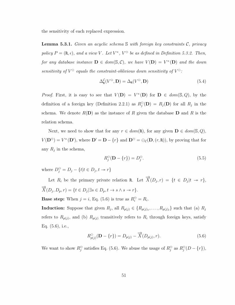
Lemma 5.3.1. Given an acyclic schema S with foreign key constraints C, privacy

policy P = (R, ε), and a view V . Let V n, V be as defined in Definition 5.3.2. Then,

for any database instance D ∈ dom(S, C), we have V (D) = V n(D) and the down

sensitivity of V equals the constraint-oblivious down sensitivity of V :

∆CR(V ,D) = ∆R(V,D) (5.4)

Proof. First, it is easy to see that V (D) = V n(D) for D ∈ dom(S, Q), by the

definition of a foreign key (Definition 2.2.1) as Rj (D) = Rj(D) for all Rj in the

schema. We denote R(D) as the instance of R given the database D and R is the

relation schema.

Next, we need to show that for any r ∈ dom(R), for any given D ∈ dom(S, Q),

V (D) = V n(D′), where D′ = D−r and D = C(D, (r, R)), by proving that for

any Rj in the schema,

Rj (D− r) = Dj . (5.5)

where Dj = Dj − t|t ∈ Dj, t r

Let Ri be the primary private relation R. Let−→X (Dj, r) = t ∈ Dj|t r,

−→X (Dj, Dp, r) = t ∈ Dj|∃s ∈ Dp, t→ s ∧ s r.

Base step: When j = i, Eq. (5.6) is true as Ri = Ri.

Induction: Suppose that given Rj, all Rp(j) ∈ Rp(j)1 , . . . , Rp(j)l such that (a) Rj

refers to Rp(j), and (b) Rp(j) transitively refers to Ri through foreign keys, satisfy

Eq. (5.6), i.e.,

Rp(j)(D− r) = Dp(j) −−→X (Dp(j), r). (5.6)

We want to show Rj satisfies Eq. (5.6). We abuse the usage of Rj as Rj (D−r),

51

Rj as Rj(D − r).

(((Rj nRp(j)1) nRp(j)2

) . . .nRp(j)`)

= (((Rj n(Rp(j)1 −−→X (Rp(j)1 , r))) nRp(j)2) . . .nR

p(j)`

)

= (((Rj −−→X (Rj, Rp(j)1 , r)) n(Rp(j)2 −

−→X (Rp(j)2 , r)) . . .nRp(j)`)

= ((Rj −−→X (Rj, Rp(j)1 , r) ∪

−→X (Rj, Rp(j)2 , r)) . . .nRp(j)`)

= Rj −−→X (Rj, Rp(j)1 , r) ∪

−→X (Rj, Rp(j)2 , r)

∪−→X (Rj, Rp(j)3 , r) . . . ∪−→X (Rj, Rp(j)` , r)

= Rj −−→X (Rj, r) (5.7)

This gives us V (D) = V n(D′). Therefore, we can have V (D)4V (D) = V n(D)4V n(D′).

Lemma 5.3.1 justifies the use of the simpler notion of sensitivity employed by

SensCalc in Section 5.2.1. Note that, for some D, V (D) 6= V (D) due to the

truncation rewrite.

Putting it all together: Given a view V , we first apply Algorithm 2 to V to add

truncation operators to the primary private relation R and obtain V τ . Then we run

semijoin rewrite in Definition 5.3.2 to get V τ,.

As the second step of semijoin rewrite introduces extra truncation operators into

the query plan, existing truncation operators may become redundant, in which case

we keep ones closest to the base relation. The following example shows the entire

procedure of a view rewrite.

Example 4. Recall the query plan V and its truncation rewrite V τ from Fig. 5.2.

Under the Household policy, Person is a secondary private relation. As shown in

Fig. 5.3 the semijoin rewrite will replace the Person relations in V τ with a semijoin

52

Primary Private Relation

Secondary Private Relation

⨝hid

γhid

πrelp, race, cnt

Sem

join

Rew

rite

Trunchid,k

⋉hid

Household

PersonTrunchid,k

⋉hid

Person

Household

Figure 5.3: Query plan of V2 view from Fig. 5.2, after adding semijoinoperators, where Household is the primary relation.

between Person and Household. Truncation operators are also added to bound the

sensitivity of the Person table to get V τ,. Note that the truncation operator in V τ

is redundant in V τ, and removed since the semijoin rewrite introduces the same

truncation operator on Person. After truncation rewrite with threshold k, SensCalc

outputs a bound on the global sensitivity: ∆R(V′2) = 2 · k2 + k.

Theorem 5.3.2 shows that after applying the truncation and semijoin rewrites the

sensitivity of V τ, output by SensCalc is the global sensitivity. Proof follows from

Theorem 5.2.1 and Lemma 5.3.1.

Theorem 5.3.2. Given an acyclic schema S = (R1, . . . , Rk) with foreign constraints

C, and R ∈ S. For any V , let V τ, denote V after applying both the truncation rewrite

(Algorithm 2) and the semijoin rewrite (Definition 5.3.2) , where the truncation

thresholds are k and are fixed. The global sensitivity of V τ, is bounded:

∆CR(V τ,) ≤ ∆R(Vτ,).

Let M be εv-differentially private algorithm that runs on V τ,(D). Then M satisfies

PV -DP with PV = (R, εv · ∆R(Vτ,)).

53

The proof follows from applying the argument of Theorem 5.2.1 with the addition

of Lemma 5.3.1. More specifically:

Proof. Part I: Let mf∞ be as defined in Lemma 5.2.2. For any D ∈ dom(S, C),

∆CR(V τ,,D)

= ∆R(Vτ,,D) (by Lemma 5.3.1)

≤ ∆R(Vτ,,mf) (by Lemma 5.2.1)

= ∆R(Vτ,, mf∞) (by Lemma 5.2.2)

= ∆R(Vτ,) (simplified notation)

Because the above bound holds for all D, it also bounds the global sensitivity.

Part II: If we run an εV -differentially private mechanism M on V τ,(D), then for

any pair (S, S ′) that differ in k records, where S, S ′ are possible output of V τ,(·),

we have | ln( M(S)M(S′)

)| ≤ (εV ·k). For any D,D′ neighbors with R is the primary private

relation, V τ,(D) and V τ,(D′) differ by at most by ∆R(Vτ,). Therefore,M satisfies

PV -DP with PV = (R, εv · ∆R(Vτ,).

5.4 Private Synopsis Generator

The PrivSynGen module produces a private synopsis of a single materialized view

on the sensitive data. The input to PrivSynGen is a materialized view V (D), a set

of linear (on V ) queries QV , and a privacy budget εV . Its output is DV , an εV -DP

synopsis of V (D), w.r.t. the materialized view V (D).

One consideration is whether to release synthetic tuples or vectors of counts. The

former is efficient in terms of representation – the vector form encodes one count

for every possible tuple in the cross product of the domains of the attributes in the

table, and is thus exponential in the number of attributes. However, the latter allows

maintaining fractional counts, which leads to lower error. In addition, vector form

54

allows the use of linear algebra based inference methods to reason across multiple

independent noisy releases, which can help answer queries not present in Q. As noted

earlier there is no constraint on the type of a synopsis returned from PrivSynGen.

For example a synopsis could be a set of tuples drawn from a distribution, or a

statistical summary of V (D).

This component is probably the most well understood as it is an instance of a

common problem studied in the DP literature – answering a set of linear queries on a

single table [ZCP+14, HMM+16, MMHM18]. Furthermore, synopsis generators can

be workload aware or workload agnostic depending on whether they optimize their

output w.r.t. a set of linear queries QV .

We use both workload-agnostic and workload-aware instances of PrivSynGen,

returning a vector of counts. More specifically, we use: W-nnls, a workload-aware

version of non-negative least squares inference [LMH+15], and the workload-agnostic

algorithms Identity and Part, the latter of which performs the partitioning step

of the DAWA algorithm [LHMW14].

Let x the vector form describing a materialized view V (D), each cell of x encodes

a different element of the cross-domain of the attributes in V and xi is the count of

tuples in V (D) with value equal to that decoding.

Identity The first synopsis generator we consider is Identity a workload agnostic

method, which takes as input the vector form of the materialized view x and outputs

x = x +ξ, where each ξi is drawn i.i.d. from Laplace(0, εV ), a Laplace distribution

with mean 0 and scale εV .

WorkloadWe now describe W-nnls (Workload non-negative least squares)[ZMK+18],

a workload aware technique that first computes y the true answers of a workload on

x, then adds noise to them and lastly uses non-negative least squares to produce a

private estimate of x. More specifically, let W be the vector form of a query workload

55

Table 5.2: Instantiations of BudgetAlloc.Name λ parameter

Naive λV = 1/|V|WSize λV = |QV |/

∑V ′∈V |QV ′ |

WSens λV = S(QV )/∑

V ′∈V S(QV ′)

VSens λV = ∆V /∑

V ′∈V ∆V ′

QV and S(W) be the workload sensitivity of W with S(W) = maxi ‖wi‖1, where

wi denotes the i-th column of W. Then W-nnls computes y = y + ξ, where each

ξi is i.i.d. drawn from Laplace(0, εV /S(W)), and returns x = arg minx0

‖Wx− y‖2.

DawaWe lastly use Dawa routine to estimate a vector of counts x. Dawa partitions

the vector space of x in continuous segments that have similar counts. Then it com-

putes count estimates for the partitions, assumes uniformity within each partition,

and lastly divides the noisy partition count to get estimates for the individual cells

in that partition. Since we never utilize the second step of Dawa our instantiation

of it is workload agnostic.

All three methods described are sensitive in the complexity of a view definition

V , as the complexity increases all methods become both intractable to use – i.e., for

views with large cross-domain it might be intractable to produce the vector form x.

Moreover, even in the case that the size of V is not prohibitive w.r.t. the vectorization

step, large view complexity leads to high cell count for x which in turn leads to high

error rates of these methods.

5.5 Budget Allocator

Recall from Definition 3.2.4 that changing a row in the primary sensitive relation R

results in changing ∆R(V ) rows in view V , where ∆R(V ) is the sensitivity of view

V . Thus, running an εV -DP algorithm on view V will satisfy (R,∆R(V ) · εV )-DP. For

56

that reason the any budget allocation strategy for materializing views needs to take

into account the sensitivity of each view.

In PrivSQL, budget allocation is performed by BudgetAlloc, which has ac-

cess to the intermediate non-private outputs of PrivSQL and returns E = εV V ∈V ,

a budget allocation that satisfies:

∑V ∈V

∆V εV ≤ ε′, (5.8)

where ∆V is an upper bound of ∆R(V ) as computed from SensCalc (see Sec-

tion 5.2.1) and ε′ is the budget allocated to view generation, i.e., ε′ = ε − εmf . The

ideal allocator would be a query fair allocator that splits the budget such that each

query of the representative workload incurs the same error. In this work, we consider

allocators of the following form:

BudgetAlloc = λV · ε/∆V ∀V ∈V

As long as ∀V ∈ V : λV ≥ 0 and∑

V ∈V λV ≤ 1 this satisfies Eq. (5.8). We use

4 strategies for budget allocation as shown in Table 5.2 – Naive divides ε equally

among views; Wsize, splits the privacy budget according to the size of QV the

partial workload of each view; Wsens allocates the privacy budget according to the

sensitivity of each QV ; and Vsens splits the privacy budget proportionally to the

sensitivity of each view.

Naive The first method we describe is More specifically, under Naive we have

∀V ∈ V : λV = 1/|V|. Under this naive allocation, views involving joins (with

typically larger sensitivities) have lower privacy budgets and thus will support query

answering with higher errors.

Workload Size Our next allocator is More specifically, ∀V ∈ mathcalV : λV =

|QV |/∑V ′∈V

|QV ′|. This allocation might be preferable in situations with highly im-

57

balanced partial workload sizes, where one view can be used to answer the majority

of queries, while other views can only answer a handful of them.

Workload Sensitivity The workload sensitivity fair allocation strategy More specif-

ically, ∀V ∈ mathcalV : λV = S(QV )/∑

V ′∈VS(QV ′ )

. In the case of significant overlap

between queries of a partial workload (in terms of tuples accessed), this technique is

similar to Wsize. However, it differs in the case where |QV | S(QV ) a case that

implies little to no overlap between queries of QV .

View Sensitivity Lastly, the view sensitivity fair Vsens allocation strategy splits

the privacy budget proportionally to the sensitivity value of each view, with high

sensitivity views receiving a higher privacy budget. More specifically, ∀V ∈ V : λV =

∆V /∑V ∈V

∆V . The goal of Vsens is to permit a more uniform error among views

regardless of their view sensitivity.

5.6 Privacy Proof

We conclude with a formal privacy statement.

Theorem 5.6.1. Given an acyclic schema S = (R1, . . . , Rk) with foreign constraints

Q and a privacy policy P = (ε, R), where R ∈ S. PrivSQL satisfies P -differential

privacy.

Proof. PrivSQL first selects and rewrites a set of views V , then allocates the

privacy budget among these views, and generates a private synopsis by execut-

ing an εV -differentially private algorithm for each view V ∈ V , which by Theo-

rem 5.3.2 ensures (R, εV ) differential privacy. From Eq. (5.8), BudgetAlloc satis-

fies∑

V ∈V ∆(V ) · εV ≤ ε′. Since the budget consumed from MaxFreqCalc is εmf

and by the sequential composition (Theorem 3.2.2), the synopsis generation phase

satisfies (R, ε)-DP, where ε = ε′ + εmf .

58

PrivSQL answers queries with these private synopses without accessing the pri-

vate database. By post-processing (a special case of sequential composition), the

privacy guarantee (R, ε)-DP does not change.

59

6

Optimizing Generation of a Single Synopsis

In this chapter we focus on PrivSynGen the module responsible for releasing a

single private synopsis given a fixed privacy budget. Remember that the input to

PrivSynGen is a triple (V (D), εV , QV ), where V (D) is the materialized view, εV a

privacy parameter associated with that view, and QV is a set of linear (to V ) queries.

As discussed in Section 5.4 this problem can be reduced to releasing query answers

on a single table under differential privacy – a well studied problem in the literature.

In the sequel we: (a) present the algorithmic landscape for releasing a synopsis of a

single table; (b) describe the challenges with selecting a suitable algorithm for a given

input (V (D), εV , QV ); and (c) propose and describe Pythia, a meta-algorithm that

automatically (and without additional privacy leaks) performs algorithm selection

for a given input.

6.1 Background & Motivation

For the remainder, we treat the materialized view V (D) as a single relational table

for which we want to answer the set of queries QV under ε-differential privacy. The

private answers to QV can then be used to construct the private synopsis of V (D)

60

as described in Section 5.4.

6.1.1 Algorithmic Landscape

For most given inputs, the algorithm with the best accuracy achievable under ε-

differential privacy is unknown. There are general-purpose algorithms (e.g. the

Laplace Mechanism [DMNS06] and the Exponential Mechanism [MT07]), which

can be adapted to a wide range of settings to achieve differential privacy. How-

ever, the naive application of these mechanisms nearly always results in sub-optimal

error rates. For this reason, the design of novel differentially-private mechanisms

has been an active and vibrant area of research [HLM12][LHMW14][LYQ][QYL13]-

[XGX12][ZCX+14a]. Recent innovations have had dramatic results: in many appli-

cation areas, new mechanisms have been developed that reduce the error by an order

of magnitude or more when compared with general-purpose mechanisms and with no

sacrifice in privacy.

While these improvements in error are absolutely essential to the success of dif-

ferential privacy in the real world, they have also added significant complexity to

the state-of-the-art. First, there has been a proliferation of different algorithms for

popular tasks. For example, in a recent survey [HMM+16], Hay et al. compared

16 different algorithms for the task of answering a set of 1- or 2-dimensional range

queries on a single table. Even more important is the fact that many recent algo-

rithms are data-dependent, meaning that the added noise (and therefore the resulting

error rates) vary between different input datasets. Of the 16 algorithms in the afore-

mentioned study, 11 were data-dependent.

Data-dependent algorithms exploit properties of the input data to deliver lower

error rates. As a side-effect, these algorithms do not have clear, analytically com-

putable error rates, unlike their simpler data-independent counterparts. When run-

ning data-dependent algorithms on a range of different relational tables (as in the

61

case of the materialized views produced by PrivSQL), one may find that error is

much lower for some tables, but it could also be much higher than other methods on

other tables, possibly even worse than data-independent methods. The difference in

error across different tables may be large, and the “right” algorithm to use depends on

a large number of factors: the number of records in the table, the setting of epsilon,

the domain size, and various structural properties of the data itself.

As a result, the benefits of recent research advances are unavailable in realistic

scenarios. Both privacy experts and non-experts alike do not know how to choose

the “correct” algorithm for privately completing a task on a given input.

6.1.2 Algorithm Selection

Motivated by this, we introduce the problem of differentially private Algorithm Se-

lection, which informally is the problem of selecting a differentially private algorithm

for a given specific input, such that the error incurred will be small.

One baseline approach to Algorithm Selection is to arbitrarily choose one differen-

tially private algorithm (perhaps the one that appears to perform best on the inputs

seen so far). We refer to this strategy as Blind Choice. As we will show later adopt-

ing blind choice does not guarantee an acceptable error for answering queries under

differential privacy. A second baseline approach is to run all possible algorithms on

the sensitive database and choose the best algorithm based on their error, we refer to

this strategy as Informed Decision. This approach, while seemingly natural, leads to

a privacy leak since checking the error of a differentially private algorithm requires

access to the sensitive data.

6.1.3 Our approach

We propose Pythia, an end-to-end differentially private mechanism for achieving

near-optimal error rates using a suite of available privacy algorithms. Pythia is a

62

Algorithm Selection

Run A* ϵ2

WD

A* Algorithm

Sensitive Database

ϵ

Pythia

Private Answers of Queries on Sensitive DB

Workload of

Queries

Feature Extractorϵ1

WDFeature-based

Algorithm Selector

Figure 6.1: The Pythia meta-algorithm computes private query answersgiven the input data, workload, and epsilon. Internally, it models theperformance of a set of algorithms, automatically selects one of them,and executes it.

meta-algorithm, which safely performs automated Algorithm Selection and executes

the selected algorithm to return a differentially private result. Using Pythia, data

curators do not have to understand available algorithms, or analyze subtle properties

of their input data, but can nevertheless enjoy reduced error rates that may be

possible for their inputs.

Pythia works in three steps, as illustrated in Fig. 6.1. First it privately extracts

a set of feature values from the given input. Then, using a Feature-based Algorithm

Selector Pythia chooses a differentially private algorithm A∗ from a collection of

available algorithms. Lastly, it runs A∗ on the given input. An important aspect of

this approach is that Pythia does not require intimate knowledge of the algorithms

from which it chooses, treating each like a black-box. This makes Pythia extensible,

easily accommodating new advances from the research community as they appear.

Our results have two important consequences. First, because our Feature-based

Algorithm Selector is interpretable, the output of training phase can provide insight

into the space of algorithms and when they work best. (See for example Fig. 6.3).

63

Second, we believe our approach can have a significant impact on future research

efforts. An extensible meta-algorithm, which can efficiently select among algorithms,

shifts the focus of research from generic mechanisms (which must work well across

a broad range of inputs) to mechanisms that are specialized to more narrow cases

(e.g., datasets with specific properties). One might argue that algorithms have begun

to specialize already; if so, then effective meta-algorithms justify this specialization

and encourage further improvements. In this section we describe the data model,

workloads, differentially private algorithms, and our error metric.

Data Model: We use the vector representation shown in Section 2.2.1. As a re-

minder, the relational table D is a multiset of records, each having k attributes

with discrete and ordered domains. We describe D as a vector x ∈ Nd where

d = d1 × . . . × dk, and dj is the domain size of the jth attribute. We denote the

ith value of x with xi.

Given a vector dataset x, we define three of its key properties: its scale is the

total number of records: sx = ‖x‖1; its shape is the empirical distribution of the

data: px = x/sx; and its domain size is the number of entries dx = |x|.

Queries A query workload is a set of queries defined on x and we use matrix notation

to define it. A query workload W is an m × d matrix where each row represents a

different linear query on x. The answer to this workload is defined as y = Wx. An

example of a workload is P, an upper triangular matrix with its non-zero elements

equal to 1. This workload is called the prefix workload and contains all prefix queries

on a dataset vector – i.e., ∀i : qi = x1 + . . .+ xi.

Usually a data curator is not interested in answering one specific workload, but

rather a collection of similar workloads. For that reason we define a task T as a

collection of relevant workloads. Examples of tasks include 1D range queries, 2D

range queries, marginal queries, etc.

64

Table 6.1: Algorithm overview for query release on single table.

AlgorithmName

Tasks PriorWork

Data IndependentLaplace General Purpose [DMNS06]Hb Range Queries [QYL13]Privelet Range Queries [XWG11]

Data DependentUniform General Purpose n/aDAWA Range Queries [LHMW14]MWEM General Purpose [HLM12]AHP General Purpose [ZCX+14a]AGrid 2d Range Queries Queries [LYQ]DPCube 2d Range Queries [XGX12]

Error Measurement For a differentially private algorithm A, dataset x, workload

W, and privacy parameter ε we denote the output of A as y = A(W,x, ε) . Then

the error is the L2 distance between the vectors of the true answers and the noisy

estimates: error(A,W,x, ε) = ‖y − y‖2

Algorithms Differentially private algorithms can be broadly classified as data-

independent and data-dependent algorithms. The error introduced by data indepen-

dent algorithms is independent of the input database instance. Classic mechanisms

like the Laplace mechanism [DMNS06] are data independent. For the task of an-

swering range queries, alternative data-independent techniques can offer lower error.

One example is Hb [QYL13], which is based on hierarchical aggregation – i.e., it

computes counts for both individual bins of a histogram as well as aggregate counts

of hierarchical subsets of the bins.

Data-dependent algorithms usually spend a portion of the budget to learn a

property of the dataset based on which they calibrate the noise added to the counts

of x. A category of data-dependent algorithms are partition-based ; these algorithms

work by learning a partitioning of x and add noise only to the aggregate counts of the

65

partitions. The value of any individual cell of x is given by assuming uniformity on its

partition. While this technique reduces the total noise added to x, it also introduces a

bias factor because of the uniformity assumption on the partitions. Hence, the overall

error greatly depends on the shape of x. Examples of data-dependent partitioning

algorithms include DAWA, AGrid, AHP, and DPCube. Other data-dependent

algorithms (like MWEM) use other data adaptive strategies.

Section 6.1.3 lists the algorithms that Pythia chooses from for answering the task

of 1- and 2-dimensional range queries.

6.2 Algorithm Selection

In this section we formally define the problem of Algorithm Selection, describe the

desiderata of potential solutions, and discuss the limitations of three baseline ap-

proaches.

Example 5. Histogram Release Suppose a medical establishment that wants

to share aggregate statistics of their medical records to teams of researchers. More

specifically, the medical researchers have requested a histogram of illnesses of all the

patients in the last year. The hospital wants to honor this request, while being careful

about any privacy leaks that such a release might have. For that reason they want

to release a differentially private version of the histogram over the diseases. The

data curator of the hospital has a basic understanding of histogram release under

differential privacy and is familiar with the literature. However and since the curator

is not a privacy expert, he has no good insight on what is the best in terms of error

algorithms to choose from.

Example 6. Multi-stage Task Suppose that a credit card company wants to offer a

new product to its clients, a credit default estimator that warns a client if their current

behavior might lead to a future credit default. The way that such a service works is

66

simple, based on historical data of their older clients, the credit card company builds

a binary classifier that it is then used by new users to estimate their probabilities

of defaulting. The input of such a model are histograms of attributes of the data

like income, past payments, demographics, etc, of past clients. Since the credit card

company does not want to compromise the privacy of their older clients, they decide to

use differential privacy to estimate the histograms before building the binary classifier.

If the credit card company uses only one algorithm to estimate all the histograms

needed, they miss on an big opportunity to improve the accuracy of the classifier,

since the set of these histograms is highly heterogeneous.

We identify two important properties of modern differentially private applica-

tions, algorithm suitability and input heterogeneity, both of which motivate algo-

rithm selection. In Example 5 we show a use case that highlights the importance

of algorithm suitability, the data curator wants to use the algorithm that provides

the highest utility. In Example 6 we illustrate that the increasing complexity of

modern differentially private systems leads to input heterogeneity, i.e., the sensitive

data is not a single histogram, but rather a collection of histograms. To address both

of these limitations, we propose using algorithm selection to choose a differentially

private algorithm before answering queries.

Algorithm selection is function over a suite of algorithms, a sensitive dataset, a

workload of queries for the dataset, and a desired privacy loss budget associated with

the query release. More specifically,

Definition 6.2.1. Algorithm Selection. Let W be a workload of queries to be an-

swered on database x under ε-differential privacy. Let A denote a set of differentially

private algorithms that can be used to answer W on x. The problem is to select an

algorithm A∗ ∈ A to answer W on x.

We identify the following desiderata for Algorithm Selection solutions: (a) dif-

67

ferentially private, (b) algorithm-agnostic, and (c) competitive.

Differentially Private: Algorithm Selection methods must be differentially private.

If the input data is relevant to an Algorithm Selection method, any use of the input

data must be included in an end-to-end guarantee of privacy.

Agnostic: Algorithm Selection methods should treat each algorithm A ∈ A as

a black box, i.e., solutions should only require that algorithms satisfy differential

privacy and should be agnostic to the rest of the details of each algorithm. Agnostic

methods are easier to deploy and are also readily extensible as research provides new

algorithmic techniques.

Competitive: Algorithm Selection methods should provide an algorithm A∗ that

offers low error rates on a wide variety of inputs (multiple workloads, different

datasets).

We measure the competitiveness of an Algorithm Selection method using a regret

measure defined to be the ratio of the error of the selected algorithm to the least

error achievable from any algorithm of A. More precisely, given a set of differentially

private algorithms A, a workload W, a dataset x, and a privacy budget ε, we define

the (relative) regret with respect to A, of an algorithm A ∈ A as follows:

regret(A,W,x, ε) =error(A,W,x, ε)

minA∈A error(A,W,x, ε)

6.2.1 Baseline Approaches

As we mentioned in Section 6.1, two baseline approaches to Algorithm Selection

are Blind Choice and Informed Decision. We also consider a third baseline, Private

Informed Decision and explain how each of these approaches violate our desiderata.

Blind Choice This baseline consists of simply selecting an arbitrary differentially

private algorithm and using it for all inputs. It is a simple solution to Algorithm

68

Selection and clearly differentially private. But such an approach will only be com-

petitive if there is one algorithm that offers minimal, or near-minimal error, on all

inputs. Hay et al. demonstrated [HMM+16] that the performance of algorithms

varies significantly across different parameters of the input datasets, like domain

size, shape, and scale. One of the main findings is that there is no single algorithm

that dominates in all cases. Our results in Section 7.2.2 confirm this, showing that

the regret of Blind Choice (for any one algorithm in A) is high.

Informed Decision In Informed Decision the data curator first runs all available

algorithms on the given input and records the error of each algorithm. He then

chooses the algorithm that performed the best. While Informed Decision solves

Algorithm Selection with the lowest possible regret, it violates differential privacy

since it needs to access the true answers in order to compute the error.

Theorem 6.2.1. There exists a set of differentially private algorithms A, an input

(W,x, ε) such that if Informed Decision is used to choose A∗ ∈ A for the input

(W,x, ε) then releasing A∗(W,x, ε) violates Differential Privacy.

Proof. Let W be a query workload and let x and y be two neighboring datasets

(i.e., ‖x − y‖1 = 1) that have distinct outputs on W. That is, Wx 6= Wy. Let

Ax and Ay be two algorithms such that Ax always outputs Wx independent of the

input, and Ay always outputs Wy independent of the input. Since Ax, and Ay are

constant functions, they trivially satisfy differential privacy for any ε value.

Consider the Algorithm Selection problem where A = Ax,Ay. For input x =

(W,x, ε) informed decision picks the algorithm that results in the least error which

is Ax. For informed decision ID to satisfy ε-differential privacy, we want ∀S ∈

Range(ID):

P (ID(x) ∈ S) ≤ exp(ε)× P (ID(y) ∈ S)

69

But we know that P (ID(x) = Wx) = 1, while P (ID(y) = Wx) = 0, resulting in

contradiction.

Private Informed Decision This strategy follows the same steps as Informed De-

cision except that estimation of the error of each algorithm is done in a differentially

private manner. Naturally, this means the total privacy budget must be split to be

used in two phases: (a) private algorithm error estimation, and (b) running the cho-

sen algorithm. This kind of approach has already been proposed in [CV13], where

the authors use this method to choose between differentially private machine learning

models.

The main challenge with this approach is that it requires that algorithm error

has low sensitivity; i.e., adding or removing a record does not significantly impact

algorithm error. However, we are not aware of tight bounds on the sensitivity of error

for many of the algorithms we consider in Section 7.1.2. This means that Private

Informed Decision cannot be easily extended with new algorithms. So, while Private

Informed Decision satisfies differential privacy and may be more competitive than

Blind Choice, it violates the algorithm agnostic desideratum.

6.3 Pythia Overview

Our approach to solve Algorithm Selection is called Pythia (see Fig. 6.1) and works

as follows. Given an input (W,x, ε), Pythia first extracts a set of features F from the

input, and perturbs each f ∈ F by adding noise drawn from Laplace(d · ∆f/ε1),

where ∆f denotes the sensitivity of f , and d is the number of sensitive features.

The set of features and their sensitivities are predetermined. Next it uses a Feature-

based Algorithm Selector (FAS) to select an algorithm A? from an input library

of algorithms A based on the noisy features of the input. Finally, Pythia executes

algorithm A? on (W,x, ε2) and outputs the result. It is easy to see that this process

70

Training

Task

Delphi: Pythia Constructor

Representative Workloads

...

Public Databases

...

DP Algorithms Repository

...

Feature ExtractorFeatures Used

Features Sensitivity

Feature-based Algorithm Selector

Figure 6.2: Delphi: Building of Pythia

is differentially private.

Theorem 6.3.1. Pythia satisfies ε-Differential Privacy, where ε = ε1 + ε2.

Proof. Feature extraction satisfies ε1-Differential Privacy and executing the chosen

algorithm satisfies ε2-Differential Privacy. The proof follows from sequential compo-

sition of differential privacy (see Theorem 2.1.1).

The key novelty of our solution is that the Feature-based Algorithm Selector is

constructed using a learning based approach, called Delphi (see Fig. 6.2). Delphi can

be thought of as a constructor to Pythia: given a user specified task T (e.g., answering

1-dimensional range queries) it utilizes a set of differentially private algorithms ATthat can be used to complete the task T , and a set of public datasets to output the set

of features F , their sensitivities ∆F as well as the Feature-based Algorithm Selector

(FAS). To learn the FAS, Delphi constructs a training set by (a) generating training

inputs (W,x, ε) that span diverse datasets and workloads, and (b) measuring the

empirical error of algorithms in AT on training inputs. Delphi never accesses the

private input database instance, but rather uses public datasets to train the FAS.

71

This allows Delphi to (a) trivially satisfy differential privacy with ε = 0, and (b) be

run once and re-used for Algorithm Selection on different input instances.

Next we describe the design of Delphi and Pythia in detail. Section 6.4 describes

the training procedure employed by Delphi to learn a Feature-based Algorithm Selec-

tor. Section 6.4.2 describes specific implementation choices for the task of answering

range queries. Section 6.5 describes the Pythia algorithm as well as optimizations

that help reduce error.

6.4 Delphi: Learning a FAS

Delphi’s main goal is to build a Feature-based Algorithm Selector (FAS) that can

be used by Pythia for algorithm selection. The design of Delphi is based on the

following key ideas:

Data Independent As mentioned in the previous section, we designed Delphi to

work without knowledge of the actual workload W, database instance x, or privacy

parameter ε that will be input to Pythia. Delphi only takes the task (e.g., answering

range queries in 1D) as input. First, this saves privacy budget that can be used for

extracting features and running the chosen algorithm later on. Secondly, this allows

the FAS output by Delphi to be reused for many applications of the same task.

Rule Based Selector The FAS output by Delphi uses rules to determine how

features are mapped to selected algorithms. In particular we use Decision Trees

[Loh11] for algorithm selection. Decision trees can be interpreted as a set of rules

that partition the space of inputs (in our case (W,x, ε) triples), and the trees Delphi

outputs shed light into the classes of (W,x, ε) for which an algorithm has the least

error. Moreover, prediction is done efficiently by traversing the tree from root to

leaf. We discuss our decision tree implementation of FAS in Section 6.4.

Supervised ApproachDelphi constructs a training set where each training instance

72

is associated with features extracted from triples (W,x, ε) and the empirical error

incurred by each A ∈ A for that triple. We ensure the training instances captures

a diverse set of ε values as well as databases x with varying shapes, scales and

domain sizes. Unlike standard supervised learning where training sets are collected,

Delphi can (synthetically) generate as many or as few training examples as necessary.

Training set construction is explained in Section 6.4.

Regret-based Learning Standard decision tree learning assumes each training in-

stance has a set of features and a label with the goal of accurately predicting the

label using the features. This can be achieved by associating each training instance

with the algorithm achieving the least error on the instance. However, standard

decision tree algorithms view all mispredictions as equally bad. In our context this

is not always the case. Recent work [HMM+16] has shown that for datasets x with

large scales (e.g. ≥ 108 records), algorithms like MWEM have a high regret (in the

hundreds), while algorithms like Hb and DAWA have low regrets (close to 2) for the

task of 1D range queries. A misprediction that offers a competitive regret should not

have the same penalty as a misprediction whose regret is in the hundreds. Towards

this goal, Delphi builds a decision tree that partitions the space of (W,x, ε) triples

into regions where the average regret attained by some algorithm is low. Delphi

does not distinguish between algorithms with similar regrets (since these would all

be good choices), and thus is able to learn a FAS that selects algorithms with lower

regret than models output by standard decision tree learning. Our learning approach

is described in detail in Section 6.4.1.

We use decision trees to implement the Feature-based Algorithm Selector. The

FAS is a binary tree where the internal nodes of the tree are labeled with a feature

and a condition of the form fi ≤ v. Leaves of the tree determine the outcome, which

in our case is the chosen algorithm. The decision tree divides the space of inputs

73

Domain <= 24

Scale <= 3072

True

NNZ <= 25

False

Dawa Laplace AGrid Hb

Figure 6.3: Example of an FAS for 2D range queries.

into non-overlapping regions – one per leaf. All inputs in the region corresponding

to the leaf satisfy a conjunction of constraints on features `1 ∧ `2 ∧ . . . ∧ `h, where

`i = (fi ≤ v) if the leaf is in the left sub-tree of an internal node with that condition,

and `i = (fi > v) if the leaf is in the right sub-tree.

Given an unseen input set of features, prediction starts at the root of the tree.

The condition on the internal node is checked. Traversal continues to the left child if

the condition is true and to the right if the condition is false. Traversal stops at the

leaf which determines the outcome. Figure 6.3 shows an example FAS for the task of

2-dimensional range queries. For instance, the FAS selects the Laplace mechanism

for inputs with small domain size (≤ 24) but a large number of records (> 3072).

Similarly, the FAS picks AGrid for large domain sizes (> 24) with a small number

of non-zero (NNZ≤ 25) counts.

Training Data For a task T , Delphi chooses a set of differentially private algorithms

AT for T . Then using a library of representative workloads for the task T and

a benchmark of public datasets, Delphi constructs a set of inputs ZT of the form

z = (W,x, ε). Details on how ZT is constructed can be task dependent, and the

implementation for range queries is described in Section 6.4.2.

74

Algorithm 4 Cart (I) [BFOS84, Loh11]1: Start at the root node, containing all training data I.2: For each feature f find the value s∗ such that splitting on (f, s∗) results in children

whose weighted average of node impurity (NI) is minimized. Repeat the processfor all features and choose (f ∗, s∗) that minimizes the weighted average of NI ofthe children.

3: Recurse on each child until the stopping criterion is met.

Next, from an input z = (W,x, ε), we extract a feature vector to be used in FAS.

Features can be derived from the workload W, the input dataset x, or the privacy

budget ε. Let F be a set of real valued functions over input triples. For f ∈ F , we

denote by fz the value of feature f on input triple z, and by fz the feature vector

[f1z , . . . , fmz ]ᵀ. Examples of features include the number of records in the dataset

(or scale), or the domain size. Section 6.4.2 describes the precise set of features used

for the task of range queries. Delphi also records the performance of each algorithm

A ∈ AT on each input z ∈ ZT and creates a regret vector for each z: rz that contains

the regret for all algorithms in AT for input z.

rz =[

regretrel(A, z)]ᵀ∀A∈AT

Finally, Delphi records the algorithm with the least error on z, say A∗z, which will

have a regret of 1. Thus, the final training data is a set I consisting of triples of

the form i = (fz,A∗z, rz). We use the notation i.fz, i.A∗z, i.rz to refer to the different

members of the training instance i.

6.4.1 Regret-based Learning

Decision trees are typically constructed in a top-down recursive manner by parti-

tioning the training instances I into a tree structure. The root node is associated

with the set of all training examples. An internal node v that is associated with a

subset of training examples V ⊂ I, is split into two child nodes vf≤s and vf>s based

on a condition f ≤ s. The children are associated with Vf≤s = i ∈ V |i.fz ≤ s

and Vf>s = i ∈ V |i.fz > s, respectively. The split condition f ≤ s is chosen by

75

computing the values f ∗, s∗ according to a splitting criterion. Recursive tree con-

struction ends when a stopping condition is met. The two conditions we consider

are: (a) when no split of the node v results in an improvement and (b) when the tree

has reached a maximum depth hmax. Algorithm 4 describes a standard decision tree

construction algorithm called Cart. Note that the computation of f ∗ implies that

features are automatically selected in order from the system.

The splitting criterion we use in this work chooses (f ?, s?) to maximize the differ-

ence between the node impurity (NI for short) of the parent node, and the weighted

average of the node impurities of the children resulting from a split.

argmaxf,s

(|V |NI(v)−

(|Vf≤s|NI(vf≤s) + |Vf>s|NI(vf>s)

))

Node impurity NI is a function that maps a set of training instances to a real number

in the range [0, 1] and measures the homogeneity of the training examples within a

node with respect to predicted values. In our context, NI(v) should be low if a single

algorithm achieves significantly lower error than all other algorithms on instances in

V , and high if many algorithms achieve significantly lower error on subsets training

examples. Decision tree construction methods differ in the implementation of NI.

We next describe four alternate implementations of NI that result in four splitting

criteria – best algorithm, group regret, minimum average regret and regret variance

criterion. As the names suggest, the first criterion is based just on the best algorithm

for each training instance (and is an adaptation of a standard splitting criterion).

The other three splitting criteria are novel and are based on the regrets achieved by

all algorithms in AT on a training instance z. In Section 7.2.4 we make a quantitative

comparison between all splitting criteria we consider.

Best Algorithm Criterion This approach treats the problem of Algorithm Selec-

tion as a standard classification problem, where each training instance is associated

76

with a label corresponding to the algorithm with the least error on that instance.

If multiple algorithms achieve a regret of 1, one of them is arbitrarily chosen. The

NI(V ) implementation we consider is the standard Gini impurity [Loh11], which

measures the likelihood that a randomly chosen training instance in V will be mis-

classified if a label was predicted based on the empirical distribution of labels in V .

More specifically, for node v of the tree let tv denote the empirical distribution over

the labels.

tv =

[1

|V |∣∣i ∈ V |s.t. i.A∗z = A

∣∣]ᵀ∀A∈AT

That is, tv[A] is the fraction of training instances for which A is the best algorithm.

The Gini impurity on node v is defined as follows:

NI(v) = Gini(v) = 1− tᵀv · tv

As discussed before, the best algorithm criterion views all algorithms that are not

the best as equally bad. Delphi employs a regret-based splitting criterion discussed

next, which allow to rank different splits based on their average regret. Recall that

i.rz denotes the vector of regrets for all algorithms A ∈ AT on training instance z.

We define the average regret vector of training instances in V as:

rv =1

|V |∑i∈V

i.rz

Group Regret Criterion We now present our best splitting criterion for algorithm

selection, which we call the Group Regret Criterion. The key idea behind this split-

ting criterion is to (a) cluster algorithms with similar average regrets for a set of

training instances, (b) associate training instances of a node v to the group of v

with the least average regret, and (c) compute the Gini impurity criterion on the

77

empirical distribution of the groups rather than on the empirical distribution over

the labels (i.e., the best algorithm). The intuition is that choosing any algorithm

from the same cluster would result in similar average regret, and thus algorithms in

a cluster are indistinguishable.

Let C a partitioning of AT , then for a node v let gvC denote the empirical distri-

bution over the clusters of C:

gvC =

[1

|V |∣∣i ∈ V |s.t. i.A∗z ∈ C∣∣]ᵀ

∀C∈C

That is, gvC [C] is the fraction of training instances for which some A ∈ C is the

algorithm that attains the least error.

Definition 6.4.1 (θ-Group Impurity). Given a node v associated with a set of train-

ing examples V and a threshold θ ∈ R+, we define a θ-clustering of algorithms

AT to be a partitioning C = C1, . . . , Ck such that ∀C ∈ C and ∀A,A′ ∈ C,∣∣rv[A]− rv[A′]∣∣ ≤ θ. The θ-Group Impurity of v is defined as:

NI(v) = GIθ(v) = minθ-clusterings C

1− gᵀvC · gvC (6.1)

For a node v, the clustering C∗ that achieves the minimum GIθ(v) is called the

θ-Group Clustering (θGC).

The intuition behind θ-Group Impurity is the following: suppose A is the best

algorithm for an instance z (regret is 1). Other algorithms A′ that are in the same

cluster in a θGC have regret at most θ + 1, and hence the model should not be

penalized for selecting A′ instead of A. However, the FAS must be penalized for

selecting algorithms that are not in the same cluster as A in the θGC.

θ-group clusterings can be efficiently computed due to the following property:

Lemma 6.4.1. Let C be a θGC for a set of algorithms in node v of the FAS. For

any three algorithms k, l, m such that rv[k] ≤ rv[l] ≤ rv[m], if k and l are in

78

the same cluster C ∈ C, then l is also in the same cluster C. Any θGC: C∗ is

regret-continuous. For C ∈ C∗ and any three algorithms k, l,m ∈ AT such that

rv[k] ≤ rv[l] ≤ rv[m] if k,m ∈ C then l ∈ C.

Before we prove Lemma 6.4.1, we extend our notation to help us with the proof.

Let a θ-clustering C, then the partial sum of a cluster Ci ∈ C is: Si = gvC [Ci]ᵀgvC [Ci],

it follows that gᵀvC · gvC =∑Ci∈C

Si. Also let g(C) = gᵀvC · gvC .

Proof of Lemma 6.4.1. We prove by contradiction. Let C∗ a θ−Group Clustering

for node v and algorithms AT . This implies that C∗ = argmaxC g(C). Assume that

C∗ does not satisfy the claim, i.e., there exist algorithms k, l,m ∈ AT such that

rv[k] ≤ rv[l] ≤ rv[m] with k,m ∈ Ci and l ∈ Cj, where Ci, Cj ∈ C∗. It is obvious

that l is admissible to Ci (since it is bounded by k and m already in Ci.

Also note that since max[h]∈Cj|rv[h]−rv[l]| ≤ θ, at least one of k,m is admissible

to Cj.

We consider two cases, regarding the partial sums of Ci and Cj. If S∗i ≥ S∗j :

we construct another solution C ′ by removing l from Cj and adding it to Ci, i.e.

C ′ = C | ∀C ∈ C\Ci, Cj ∪ Cj\l ∪ Ci ∪ l. The value of this solution is

computed as follows:

g(C ′) = g(C∗)− S∗2i − S∗2j + S ′2i + S ′2j

= g(C∗)− S∗2i − S∗2j + (S∗i + tv[l])2 + (S∗j − tv[l])2

= g(C∗) + 2tv[l]2 − 2tv[l]S∗j + 2tv[l]S∗i

= g(C∗) + 2tv[l]2 + 2tv[l](S∗i − S∗j ) ≥ g(C∗)

If S∗i ≤ S∗j : w.l.o.g. assume only k is admissible to Cj, then we construct C ′ by

removing k from Ci and adding it to Cj, i.e. C ′ = C | ∀C ∈ C\Ci, Cj ∪ Cj ∪

79

k ∪ Ci\k. The value of this solution is computed as follows:

g(C ′) = g(C∗)− S∗2i − S∗2j + S ′2i + S ′2j

= g(C∗)− S∗2i − S∗2j + (S∗i − tv[k])2 + (S∗j + tv[k])2

= g(C∗) + 2tv[k]2 + 2tv[k]S∗j − 2tv[k]S∗i

= g(C∗) + 2tv[k]2 + 2tv[k](S∗j − S∗i ) ≥ g(C∗)

As a consequence of Lemma 6.4.1, if the algorithms in AT are sorted in increasing

order of their regrets, then the θGC always corresponds to a range partitioning of the

sorted list of algorithms. More precisely, if A1,A2, . . . are such that rv[Ai] ≤ rv[Aj]

for all i ≤ j, then every cluster C ∈ C∗ is a range [k,m] such that ∀` ∈ [k,m] : A` ∈ C.

When the cardinality of AT is low (like in our experiments) one can enumerate over

all the range partitions of the sorted list of algorithms to find the θGC. In cases

where AT is large we can use dynamic programming (like in [JKM+98]) since the

optimization criterion (Equation 6.1) satisfies the optimal substructure property.

Minimum Average Regret Criterion With minimum average regret (MAR) cri-

terion our goal is to promote splits in the tree where the resulting average regret of

the children is less than the average regret of the parent node. This is achieved by

choosing a Node-Impurity that measures the average regret of the node:

NI(v) = MAR(v) =‖rv‖1|AT |

Regret Variance Criterion The next criterion we consider is to promote splits

where the variance of the regret vectors of the children is smaller than the variance

of the regret of the parent node. In this case Node-Impurity(v) is simply the

variance of v:

NI(v) = Var(v) =1

|AT |∑A∈AT

(rv[A]− ‖rv‖1|AT |

)280

6.4.2 Delphi for Range Queries

In this section we present how Delphi generates the set of input instances ZT =

(W,x, ε) for tasks of range queries. Section 6.4.2 details how we generate x’s, and

Sections 6.4.2 and 6.4.2 explain how we handle workloads and epsilon values in the

training phase.

Generating Datasets

Recent work [HMM+16] on the empirical evaluation of differentially private algo-

rithms for answering range queries identified that algorithm error critically depends

on three parameters of a dataset x: scale, shape, and domain size. The characteris-

tics of the input to Pythia are not know a priori, thus we must ensure that Delphi

creates training data that spans a diverse range of scales, shapes, and domain sizes.

Delphi starts with a benchmark of public datasets Dpublic. One or two dimen-

sional datasets are constructed by choosing one or two attributes from the dataset,

respectively. For each choice of attribute(s), if the domain is categorical it is made

continuous using kernel density estimation. This process results in an empirical den-

sity, which we call the shape p. We denote by P the set of all shapes constructed.

Next, the continuous domain is discretized using equiwidth bins (in 1- or 2-

dimensions) to get various domain sizes. We denote by K the set of domain sizes for

each shape. Finally, to get a dataset of scale s, given a domain size k and shape p,

we scale up the shape p by s to get a total histogram count of s. The set of scales

generated is denoted by S. Thus the space of all datasets corresponds to P ×K×S.

We denote by X the resulting set of datasets.

Workload Optimization

Replicating training examples for every possible workload for a given task would make

training inefficient. Hence, we use the following optimization. Delphi maps each task

81

T to a set of representative workloads WT , which contains workloads relevant to the

task. For example if T is “Answer range queries on 1D datasets", then WT contains

I and P, the identity and prefix workloads respectively. The identity workload is

effective as answering short range queries, while the prefix workload is a better choice

for answering longer random range queries. Given a new task T , Delphi selects a set

of differentially private algorithms AT , a set of representative workloads WT , and

a privacy budget ε. Delphi also generates a set of input datasets X (as described

above).

For every workload W ∈ Wt Delphi generates a set of training instances IWby running all algorithms of AT , for all datasets x ∈ X , workload W, and privacy

budget ε. Then Delphi uses the Cart algorithm with training data IW and creates

a set of FAS’s: FASW | ∀W ∈ WT. Lastly, Delphi creates a root r connecting

each FASW where edges incident to r have rules based on workload features. The

resulting tree with root r is the FAS returned by Delphi.

Privacy Budget Optimization

As with workloads, Delphi could train different trees for different ε values. However,

this would either require knowing ε (or a range of ε values) up front, or would require

building an infinite number of trees. Delphi overcomes this challenge by learning a

FAS for a single value of ε = 1.0; i.e., all training instances have the same value

of ε. At run-time in Pythia, if z = (W,x, ε′), where ε′ 6= ε, Pythia transforms the

input database x to a different database x′ = ε′

εx, and runs algorithm selection on

z′ = (W,x′, ε). This strategy is justified due to the scale-epsilon exchangeability

property defined below.

Definition 6.4.2. Scale-epsilon exchangeability [HMM+16] Let p be a shape, W a

workload. For datasets x1 = s1p and x2 = s2p, a differentially private algorithm

A is scale-epsilon exchangeable if error(A,W,x1, ε1) = error(A,W,x2, ε2) whenever

82

ε1s1 = ε2s2.

Recent work [HMM+16] showed that all state-of-the-art algorithms for answering

range queries under differential privacy satisfy scale-epsilon exchangeability. We can

show that under asymptotic conditions, the algorithm selected by a FAS on (W,x, ε′)

that is trained on input instances with privacy parameter ε′ would be identical to

algorithm selected by a FAS′ on (W, ε′

εx, ε) trained on input instances with privacy

parameter ε.

Let X be P×K×R+ a set of datasets. We construct inputs Z1 = (W,x, ε1)|∀x ∈

X and Z2 = (W,x, ε2)|∀x ∈ X. We construct I1 and I2 by executing epsilon-

scale exchangeable algorithms A, on Z1 and Z2 respectively. Let the Feature-based

Algorithm Selectors constructed from these training datasets: FAS1 = Cart(I1),

and FAS2 = Cart(I2).

Theorem 6.4.1. Consider instances z1 = (W,x1, ε1) and z2 = (W,x2, ε2) such that

ε1x1 = ε2x2. During prediction, let the traversal of z1 on FAS1 result in leaf node v1,

and let the traversal of z2 on FAS2 result in leaf node v2. Then, we have tv1 = tv2.

Thus, the algorithm selected by FAS1 on z1 is the same as the algorithm selected by

FAS2 on z2.

We prove Theorem 6.4.1 after showing the following lemma. Recall that in Sec-

tion 6.4.2 we defined FAS1, and FAS2 trained on infinite training sets, with different

epsilon values. We also define a ε-stable bijection. A bijection fε,ε′ : D → D is a ε-

stable bijection if for fε,ε′(s ·p) = s′ ·p, any workload W, and a scale/ε-exchangeable

algorithm A:

error(A,W, sp, ε) = error(A,W, s′p, ε′)

Lemma 6.4.2. Let fε,ε′ an ε-stable bijection. We denote the nodes of FAS1 at level

i as vi1, . . . , vi2i, and similarly for FAS2: wi1, . . . , wi2i. Then ∀i, j: V ij = f [W i

j ] and

tvij = twij

83

Algorithm 5 Pythia(W,x, ε, ρ)

1: ε1 = ρ · ε2: ε2 = (1− ρ) · ε3: d = Nnz(∆F)4: fz = F(W,x, ε)5: fz = fz + ∆FT Lap(d/ε1)

6: A∗ = FAS(fz)7: y = A∗(W,x, ε2)8: return y

Proof. The infinite size of the training data as well as the scale/ε exchangeability of

the algorithms in the labels guarantee that both roots of FAS1 and FAS2 share the

same label distribution. Consider the first split of FAS1: (v1, v2), we know that this

split achieves the highest impurity improvement: θ1. We argue that the first split of

FAS2 : (W1,W2) is such that V1 = f [W1], V2 = f [W2], if it was any other case then

the impurity improvement would be less in either FAS1, or FAS2. Because of f is an

ε-stable bijection this also implies that tv1 = tw1 and tv2 = tw2 . As tree construction

is made top-down, we recursively apply the same argument and the proof follows.

Proof. [Theorem 6.4.1] From Lemma 6.4.2 we have that all non-leaf nodes vij and

wij make a split on the same feature, more specifically ∀f ∈ F\scale : the split

condition is the same, and that for f = scale the split conditions are of the form

(f, s) and (f, sε1/ε2) for FAS1 and FAS2 respectively.

This means that at traversal time, z1 and z2 will end up in the leaves vij and wij

of FAS1, and FAS2. The proof follows from Lemma 6.4.2.

6.5 Deploying Pythia

Pythia is a meta-algorithm with the same interface as a differentially private algo-

rithm: its input is a triple z = (W,x, ε), and its output is y, the answers of W on

x under ε-differential privacy. Pythia works in three steps: feature extraction, algo-

84

rithm selection, and algorithm execution. First, using ε1 privacy budget it extracts

a differentially private estimate of the features fz from the input z. Then based on

fz it uses its FAS to choose an algorithm A∗, which runs with input (W,x, ε2) and

returns the result.

In Algorithm 5 we see an overview of Pythia. In lines 2-3 of Algorithm 5 we

split the privacy budget to ε1 and ε2 to be used for feature extraction and algorithm

execution, respectively. In line 4 we compute the number of total features that need

to be privately computed (Nnz is a function that returns the number of non-zero

elements of a given vector). In line 5 we extract the true features fz and in line 6 we

use the Laplace Mechanism to produce a private estimate fz. In line 7 we apply

the FAS on the noisy features fz and we get the chosen algorithm A∗. In line 8 we

run A∗ with input z = (W,x, ε2) and return the answer.

Feature Extraction Delphi provides Pythia with the set of features F of the input

z = (W,x, ε). As a reminder, features extracted from the sensitive dataset x might

potentially leak information about x; for that reason we need to privately evaluate

the values of these features on x. To do so, we use the vector of sensitivities ∆F of

each individual feature. We add noise to the features in the following manner: we

assign a privacy budget ε1 for feature extraction, and then use the Laplace Mechanism

to privately evaluate each feature’s value by using a fraction ε1/d for each feature,

where d is the total number of sensitive features. This process guarantees that feature

extraction satisfies ε1-differential privacy.

6.5.1 Deployment Optimizations

The first optimization we consider is dynamic budget allocation, and the second is

post-processing via noisy features. In Algorithm 6 we show Pythia utilizing both

optimizations. We now give an overview of each optimization.

85

Algorithm 6 Pythia(W,x, ε, ρ) – w/ Optimizations1: ε1 = ρ · ε2: ε2 = (1− ρ) · ε3: d = Nnz(∆F)4: fz = F(W,x, ε)5: fz = fz + ∆FT Lap(d/ε1)

6: A∗, f ′z = FAS(fz)7: ε′2 = ε2 + (d− |f ′z|)/dε18: y = A∗(W,x, ε′2)

9: y = Optimize(y,W, f ′z)10: return y

Dynamic Budget Allocation The first optimization we consider is to dynamically real-

locate the privacy budget between feature extraction and the execution of the selected

algorithm. Recall that the feature extraction step of Pythia consumes privacy budget

ε1 to recover d sensitive features from x. Then fz is used to traverse the decision tree

FAS to choose an algorithm A∗. In reality, not all features are necessarily used at

the tree traversal step. For example, in Fig. 6.3, while there are 2 sensitive features

(scale, number of non-zero counts) in the FAS, any input traversing that FAS will

only utilize one sensitive feature (either scale, or Nnz). In this example we have

spent ε1/2 to extract an extra sensitive feature that we do not use.

Dynamic Budget Allocation recovers the privacy budget spent on extracting fea-

tures that are not utilized in the tree traversal step and instead spends it on running

the chosen algorithm A∗. More specifically, given d′ < d sensitive features were used

to traverse the tree, we update the privacy budget of the algorithm execution step

to ε′2 = ε2 + (d − d′)/d · ε1. Lines 7 and 8 of Algorithm 6 reflect this optimization.

In the example of Fig. 6.3 this means that we will run the chosen algorithm with

privacy budget ε2 + ε1/2 and thus achieve higher accuracy on the release step.

Post-Processing via Noisy Features The second deployment optimization we propose

is a post-processing technique on the noisy output y of Pythia by reusing the noisy

86

features. The intuition behind our method is the following, the true features ex-

tracted from the dataset fz impose a set of constraints on the true answers of the

workload y. We describe these constraints as a set C, i.e., y ∈ C. Since y is a noisy

estimate of y, it might be the case that y /∈ C. In the case that C is a convex set, we

can project the noisy answer to C and get another estimate: y = ProjC(y), where

ProjA(x) , arg miny∈A ‖x − y‖. Doing this guarantees that the error of y will be

smaller than y.

Theorem 6.5.1. Let a convex set C, and points y, y′ where y ∈ C. Then ‖y −

y∗‖2 ≤ ‖y − y′‖2 where y∗ = ProjjC(y′).

At deployment time we do not know the true features fz, instead we have a noisy

estimate fz. We overcome this challenge by creating a relaxed convex space C based

on the noisy features and project to that. As an example, consider dataset x and

workload W = I the identity workload, at run-time suppose that the scale sz is used.

Then we create the constraint ‖y‖1 ≤ sz + ξ, where ξ ∼ 1/ε1 is a slack parameter, to

account for the noise added. Lastly we project the noisy answer y to space defined

by our constraint. We show experimentally significant improvements in the quality

of the final answer y using this technique.

87

7

Empirical Evaluation

In this chapter we present our experimental evaluation of the systems presented in

this thesis. We evaluate our systems using both real and benchmark datasets on a

variety of different use cases. Our main focus is reporting the error incurred for a

given privacy level. More specifically, we evaluate the end-to-end performance of the

proposed systems in a variety of different settings – i.e., privacy levels, workload size,

data size, etc. Additionally, we compare our proposed algorithms with the current

state-of-the-art competitor algorithms, showing improvements over prior work. We

also perform a system analysis of both PrivSQL and Pythia, by changing each

factor one at a time and controlling the input configurations.

The chapter is divided in two distinct sections, in Section 7.1 we present the

empirical evaluation of PrivSQL and in Section 7.2 the evaluation of Pythia. In

Section 7.1.2 we present the end-to-end error evaluation of PrivSQL on a real world

use case and a benchmark, for the former we show that for more than 60% of the

queries evaluated PrivSQL offers less than 10% relative per query error. In Sec-

tion 7.1.3, we compare PrivSQL with prior work (Flex[JNS18]) where we show

that PrivSQL offers an average case improvement in total error incurred of 2 orders

88

of magnitude – which can go up to 10 orders of magnitude for certain queries. Our

comparison with extends by running PrivSQL in “single query mode”, where again

we show improvements of at least 2 orders of magnitude across all queries. Lastly, in

Section 7.1.4 we evaluate alternative choices for components of PrivSQL and offer

an evaluation on the effect of truncation in the overall error incurred.

In Section 7.2.2 we evaluate Pythia for answering a workload of queries on 1-

and 2-dimensional datasets. Our main finding is that across a multitude of inputs

Pythia offers on average 60% improvement against the best “blind choice” algorithm

– i.e., using the same algorithm across all inputs. In Section 7.2.3 we use Pythia

as a building block for implementing a differentially private naive Bayes classifier

(NBC), where we show Pythia offers competitive misclassification rates with that of

a non-private baseline.

7.1 PrivSQL Evaluation

We evaluate PrivSQL on both a use case inspired by U.S. Census data releases

as well as the TPC Benchmark H(TPC-H)[TPC93]. In Section 7.1.2 we present

an end-to-end error evaluation analysis. In Section 7.1.3, we compare with prior

work (Flex[JNS18]). Lastly, in Section 7.1.4 we evaluate alternative choices for

components of PrivSQL.

7.1.1 Setup

Table 7.1 summarizes settings with defaults in boldface.

Datasets: We use the public synthetic U.S. Census dataset [SASV17] with the fol-

lowing schema: person(id, sex, gender, age, race, hid) and household(hid,

location). We create two datasets from the full Census data by filtering on loca-

tion: CensusPM limits to a specific PUMA region (a region roughly the size of a

town) and CensusNC limits to locations within North Carolina. CensusPM con-

89

Table 7.1: PrivSQL and input options used.Census Input Options

Dataset CensusNC , CensusPMPrivacy Policy Person, HouseholdPrivacy Budget ε 2.0, 1.0, 0.5, 0.25, 0.125Representative Workload W1, W2, W ′1, W ′2Query Workload W1, W2

TPC-H Input Options

Dataset TPC-HPrivacy Policy CustomerPrivacy Budget ε 2.0, 1.0, 0.5, 0.25, 0.125Representative Workload W3

Query Workload W3

PrivSQL Config. Options

BudgetAlloc WSize, WSens, Naive, VSensPrivSynGen W-nnls, Identity, Part

tains 50K and 38K tuples in Person and Household respectively, while CensusNC

contains 5.4M and 2.7M tuples, resp. We also use the TPC-H benchmark with a

schema consisting of 8 relations. We scaled the data to 150K, 1.5M , and 6M tuples

in the Customer, Order, and Lineitem tables respectively.

Policies: We use two policies for the Census schema, (Person, ε) and (Household, ε)

where the private object is a single individual, or a household, respectively. For

the TPC-H schema we used (Customer, ε) policy, which protects the presence of

customers in the database.

Workload: Summary File 1 (SF-1)[Cen10] is a set of tabulations released by the

U.S. Census Bureau. We parsed their description and constructed two workloads of

SQL queries: W1 and W2. W1 contains 192 complex queries, most of which contain

joins and self joins on the base tables Household and Person as well as correlated sub-

queries. An example query is the “Number of people living in owned houses of size 3

where the householder is a married Hispanic male.” The second workload W2 ⊃ W1

includes an additional 3, 493 linear counting queries on Person relation. An example

90

Table 7.2: View Statistics for queries of W2.

Person policy Household policy

View # of Sens Median Sens MedianGroup Queries Bound Qerror Bound Qerror

#1 23 0 0.0 1 948.1#2 3575 1 85.4 4 400.6#3 25 2 636.4 8 30,474.2#4 8 4 5,916.6 16 8,484.8#5 12 6 5,294.7 24 42,056.4#6 6 17 17,362.2 68 34,670.4#7 36 25 8,413.9 100 40,860.3

linear query is the “Number of males between 18 and 21 years old.”. For evaluation of

TPC-H we used queries q1, q4, q13, q16 from the benchmark to derive W3 a workload

of 61 queries, by expanding on the group by clause of the original queries.

PrivSQL configuration: The synopsis generation and budget allocation are con-

figurable, as described in Section 5.4 and listed in Table 7.1. For the LearnThresh-

old algorithm described in Section 5.2.3, we set threshold as θ = 0.9 and budget as

εmf = 0.05 · ε.

Error Measurement: For a query q, let y = q(D) be its true answer, and y be

a noisy answer, we define the absolute error of y, as: Qerror(y, y) = |y − y|.

Similarly, we define the relative error as: RelError(y, y) = |y − y|/max(50, y).

In all experiments, we run each algorithm for 10 independent trials and report the

average of the error function.

7.1.2 Overall Error Analysis

We evaluate PrivSQL on datasets CensusPM and CensusNC using workloads W1

and W2 and both Person and Household. Then we evaluate on TPC-H with the W3

workload and Customer policy.

91

All Queries 0 – 103 103 – 104 > 1040

10−4

10−3

10−2

10−1

100

101

102

Rel

ativ

eEr

ror

(a) W1, Person, CensusNC

All Queries 0 – 103 103 – 104 > 1040

10−4

10−3

10−2

10−1

100

101

102

Rel

ativ

eEr

ror

(b) W1, Household, CensusNC

All Queries 0 – 103 103 – 104 104 – 105 > 1050

10−4

10−3

10−2

10−1

100

101

102

Rel

ativ

eEr

ror

(c) W2, Person, CensusNC

All Queries 0 – 103 103 – 104 > 1040

10−2

10−1

100

101

Rel

ativ

eEr

ror

(d) W3, Customer, TPC-H

Figure 7.1: Relative error rates of PrivSQL. Top is W1 on the CensusNCdataset for Person and Household policies. Bottom is W2 on CensusNCfor Person policy and W3 on the TPC-H. Error rates stratified by truequery answer size.

Error Rates: Figs. 7.1 and 7.2 summarize the RelError distribution of PrivSQL

across different input configurations, stratified by the true query answer sizes. In each

figure we draw a horizontal solid black line at y = 1, denoting relative error of 100%.

A mechanism that always outputs 0 would achieve this error rate.

PrivSQL achieves low error on a majority of the queries. For the Person pol-

icy and CensusNC dataset (Figs. 7.1a and 7.1c), PrivSQL achieves at most 2%

92

All Queries 0 – 102 102 – 103 > 103

Query Range

0

10−2

10−1

100

101

102

Rel

ativ

eEr

ror

(a) W1 on CensusPM .

0.125 0.25 0.5 1.0 2.0

Total Budget ε

0

10−4

10−3

10−2

10−1

100

101

102

Rel

ativ

eEr

ror

(b) W1 on CensusNC .

Figure 7.2: Relative error rates for CensusPM dataset (left), as well asfor different ε values (right), both under Person policy.

RelError on 75% of the W1 queries and at most 6% RelError on 50% of the

W2 queries. For the Household policy (Fig. 7.1b) all error rates are increased. The

noise necessary to hide the presence of a household is much larger as removing one

household from the dataset affects multiple rows in the Person table. PrivSQL also

offers high accuracy answers for the W3 workload on the TPC-H benchmark, where

more than 60% of the queries achieve less than 10% relative error(Fig. 7.1d).

Fig. 7.2a shows error on the CensusPM dataset, using workload W1 workload

and Person policy. The trends are similar to the CensusNC case, but the error is

higher as query answers are significantly smaller on CensusPM than on CensusNC .

Fig. 7.2b shows more results on the CensusNC , across varying ε values. As ex-

pected, PrivSQL incurs smaller error higher values of ε. We omit figures for other

configurations due to space constraints.

Queries with smaller true answer sizes and higher sensitivity incur high error. We

discuss these effects next.

Error vs Query Size: In Fig. 7.1 and Fig. 7.2a the results are grouped by the

93

size of the true query answer. The number of workload queries in each group is

0 − 103 : 24, 103 − 104 : 73,>104 : 93 for W1 and 0 − 103 : 1869, 103 − 104 :

811, 104 − 105 : 742,>105 : 253 for W2. Queries with size <103 have the highest

error. As the true answer size increases, the error drops by an order of magnitude.

Under the Person policy, 95% of queries in W1 and W2 with size >103 have error

<10%. The median error for queries in W1 with true answer >104 is <.1%. This

further highlights the real-world utility of PrivSQL.

High error rates are mostly caused by queries with small true answer. Moreover,

we observe a dramatic downwards error trend as the size increase for both W1 and

W2. For instance, in the case of W1, 95% of queries with size > 1, 000 have error rate

less than 10% and 75% of queries with size > 100k have error less than 0.1%. These

results further highlight the applicability of PrivSQL on an employment in a real

world scenario.

View Sensitivities: In Table 7.2 we show statistics about the views generated

from PrivSQL for workload W2, dataset CensusNC , and both Person and House-

hold policies. Rows of the table correspond to groups of views that have the same

sensitivity. The second column shows the number of queries that are answerable

from views in the group. The rest of the table summarizes the sensitivity of views

in each group and the median absolute error (QError) across queries answerable

from these views under Person and Household policy, resp. For instance, there are

3575 queries answerable by views with sensitivity 1 under Person policy, and have a

median absolute error of 85.

We see that as the view sensitivity of a group increases so does the median

QError across queries. The connection is not necessarily linear due to choices

in PrivSynGen and BudgetAlloc. We also see that, for the same group, the

Household policy leads to higher sensitivity bounds and higher error rates. This is

94

because the removal of a single row in the Household table affects multiple rows in

Person.

We also derived the equivalent view statistics for TPC-H. For W3 PrivSQL

creates 4 views with computed sensitivities: 0, 104, 182, 390 and QError values are:

0, 111, 112K, 3.5K respectively. Again we see that the sensitivity to error connection

is non-linear due to factors like truncation.

7.1.3 Comparison with Prior Work

We next compare with Flex [JNS18], though a direct comparison is difficult for

several reasons. Flex is designed for answering one query at a time, while PrivSQL

answers multiple queries under a common budget. Flex satisfies (ε, δ)-differential

privacy, a relaxation of DP, whereas for PrivSQL, δ = 0. PrivSQL supports

multiple privacy policies, while Flex does not (and specifically cannot support the

Household policy). We set δ = 1/n for Flex, where n is the number of rows in the

Person table, and consider the Person policy.

For our first comparison, we compare PrivSQL against BaselineFlex, a natural

extension of Flex adapted for answering a workload of queries, where the privacy

budget is evenly divided across the set of answered queries. Then, we provide a more

direct “apples to apples” comparison by (a) running both systems one query at a

time and (b) comparing their sensitivity engines.

Workload Query Answering We evaluate performance on workloads W1 and W2

on CensusNC dataset. Flex does not support 42 queries of W1, which are complex

queries containing correlated subqueries. We omit these from the evaluation. In

Fig. 7.3 we present the results, with error distributions again stratified by query size.

We draw a solid black line at RelError = 1, which corresponds to the error of the

“just report zero” baseline [McS18]. For the W1 workload, the BaselineFlex relative

error rate exceeds 1 for more than 75% of the queries, while PrivSQL has error less

95

All Queries 0 – 103 103 – 104 > 10410−410−210

010

210

410

610

81010

1012

1014

1016

Rel

ativ

eEr

ror

PRIVSQL

BASELINEFlex

(a) W1 Workload

All Queries 0 – 103 103 – 104 104 – 105 > 10510−410−210

010

210

410

610

810

1010

12

(b) W2 Workload

Figure 7.3: Relative error comparison between PrivSQL andBaselineF lex for workload answering on the CensusNC dataset.

than 2% for 75% of the queries. Even for large query sizes (> 104), BaselineFlex

has high error rates, as W1 mostly contains complex queries with high sensitivity. In

the case of small query size we can see that PrivSQL has significantly lower error

than BaselineFlex and offers an improvement over the all-zeros baseline on half the

queries. For the W2 workload (Fig. 7.3b) the trends are similar.

The above experiments compare the systems in terms of error on an entire work-

load. One factor that contributes to PrivSQL achieving comparably lower error

than the baseline extension of Flex is that it has more sophisticated support for

workloads: VSelector groups together queries which may compose parallely and

enjoy a tighter privacy analysis, and techniques like W-nnls in the synopsis gener-

ator use least squares inference to further reduce the error of query answers.

Single Query Answering As discussed earlier, Flex is designed as an on-line

query answering system where each query is privately estimated and returned to the

user separately under its own privacy guarantee εq. To provide a more direct compar-

ison with Flex, we run our system in “single query mode”, denoted by PrivSQLsqm,

96

which takes as input a workload containing a single query and returns a private syn-

opsis to answer that query. We evaluate both systems on workloadW1 on CensusNC

and Person policy and use a per-query budget of εq = 0.01. We omit showing results

for queries in W2 \W1 as those queries have the same sensitivity, and hence same

error under both systems.

This evaluation allows us to decouple error improvements due to workload-related

components – such as VSelector, BudgetAlloc, and PrivSynGen – and focus

on the query analysis components SensCalc and VRewrite.

Fig. 7.4 shows for each query the QError of Flex on the y-axis and the QEr-

ror of PrivSQLsqm on the x-axis. Queries are grouped together w.r.t. their com-

puted sensitivity under SensCalc. Groups #6 and #7 are queries with correlated

subqueries and are unsupported by Flex. However, for illustration purposes, we

allow Flex to use the de-correlation techniques of VSelector in order to answer

them. All queries lie over the dotted x = y diagonal line, i.e., for every query,

PrivSQLsqm offers lower error than Flex. This improvement is over 10 orders of

magnitude for some Flex supported queries (Group 5). All improvements are due

to two factors: (a) the tighter sensitivity bounds of SensCalc compared with Flex

rules and (b) the VRewriter truncation technique which helps bound the global

sensitivity, avoiding the need for smoothing.

Next, we isolate the sensitivity engines of both Flex and PrivSQL and compute

only the sensitivity bounds (without truncation or smoothing). In Fig. 7.5 we show

our results using the same groups as Fig. 7.3. For all queries SensCalc offers a

strictly better sensitivity analysis with improvements ranging up to 37× on Flex

supported queries. For group #2 that contains > 40% of the W1 queries, SensCalc

offers an improvement of 4×.

97

010

210

310

410

5

PRIVSQLSQM

102

104

106

108

1010

1012

1014

1016

FLE

X-S

M

Group 1Group 2Group 3Group 4Group 5Group 6Group 7

Figure 7.4: Comparing QErrorrates of of single queries from theW1 workload on CensusNC.

#1 #2 #3 #4 #5 #6 #7View Group

0

101

102

103

104

Sens

itiv

ity

Boun

d

0 1 24

6

3349

1

8 8

96

1088 1088

11904SENSCALC RulesFLEX Rules

Figure 7.5: Comparison of Flexand PrivSQL sensitivity enginesfor queries of W1 workload.

7.1.4 System Analysis

Next, we perform a series of experiments evaluating the performance of PrivSQL

with different BudgetAlloc and PrivSynGen options. In Fig. 7.6 we show re-

sults of PrivSQL where we change component instantiations one-at-a-time in order

to better understand their impact. We also analyze the effect of the truncation op-

eration in terms of overall error (see Fig. 7.7). The next evaluations are on workload

W1 on CensusNC and Person policy.

Effect of Budget Allocator: In Fig. 7.6a we show the absolute error distribution

of PrivSQL for different BudgetAlloc choices. Wsize and Wsens offer the

best error rates, with comparable performance. This is due to low composition

parallelism between queries of each partial workload QV . High error rate queries

perform similarly across BudgetAlloc instantiations. This further explains that

Naive outperforms Vsens, as the latter assigns a larger privacy budget to high

sensitivity views, for which their sensitivity dominates the error factor.

Effect of Synopsis Generator: In Fig. 7.6b we show the absolute error distribution

of PrivSQL for different PrivSynGen choices. For representative workload W1

98

WSIZE(Default)

WSENS NAIVE VSENS0

101

102

103

104

105

106

Abs

olut

eEr

ror

(a) BudgetAlloc choices.

W-NNLS(Default)

IDENTITY PART W-NNLS (W ′1)0

101

102

103

104

105

106

(b) PrivSynGen choices.

Figure 7.6: Distribution of absolute error for different instantiations ofPrivSQL (a) shows the effect of BudgetAlloc and (b) of PrivSynGen.

(left of the dotted line), we see that W-nnls outperforms the other 2 methods. The

non-negative least squares inference technique offers significant advantage since it

optimizes for the exact queries that the analyst submits.

Effect of Representative Workload: We create W ′1, a smaller representative

workload of 35 queries that capture the join structures of queries in W1 The change

in representative workload only affects the W-nnls synopsis generator, as Identity

and Part are workload agnostic (Section 5.4). The results show that the performance

of W-nnls deteriorates whenW ′1 is used instead ofW1 (Fig. 7.6b, right of the dotted

line). This suggests that data owners with little knowledge about analyst queries may

prefer to instantiate PrivSQL with Identity or Part.

Effect of Representative Workload: We create W ′1 and W ′

2, two smaller repre-

sentative workloads that can be used to answer queries fromW1 andW2 respectively.

In Fig. 7.6b we show results for W ′1 alone, which contains 35 queries. Results for

W ′2 are omitted due to space constraints. As discussed in Section 5.4, Identity

and Part are workload agnostic, while W-nnls is workload aware. For that reason,

99

1(90%)

2(52%)

3(38%)

4(18%)

6(4%)

10(0.1%)

20(0%)

Truncation ValuePercentage of Removed Tuples

0

101

102

103

104

105

106

Abs

olut

eEr

ror

(a) Absolute error.

1(90%)

2(52%)

3(38%)

4(18%)

6(4%)

10(0.1%)

20(0%)


0

101

102

103

104

105

106

Abs

olut

eBi

as

(b) Absolute bias.

Figure 7.7: Error and bias distributions of truncation-affected queries,for different truncation values. Numbers in parentheses denote the per-centage of tuples truncated at the corresponding value.

we only show W-nnls for input W ′1 (right of the dotted line), since Identity and

Part have identical error rates for either W1 or W ′1 representative workloads.

The performance of W-nnls(W ′1) deteriorates and now both Part and Iden-

tity offer better error rates that are comparable to that of W-nnnls(W1). This

allows data owners with little to no knowledge about analyst queries to instantiate

PrivSQL with Identity or Part with little loss in analyst accuracy.

Effect of Truncation Operator: The truncation rewrite operation of VRewriter

might introduce bias in the synopses generated – due to tuples being dropped from

the base tables. To quantify this bias, we isolate the queries for which Algorithm 2

adds a truncation operator in the query plan of their corresponding view. For all

queries in our workloads, the truncated attribute is hid in Person and in PrivSQL

the LearnThreshold as described returns w.h.p. a threshold value of 4. For those

queries and for different truncation levels, we measure their total error as well as

their bias due to the addition of truncation in their corresponding views. In Fig. 7.7

we summarize our results. In both figures the x-axis is labeled by the truncation

100

1(90%)

2(52%)

3(38%)

4(18%)

6(4%)

10(0.1%)

20(0%)


10−3

10−2

10−1

100

101

102

Rel

ativ

eEr

ror

(a) Relative error.

1(90%)

2(52%)

3(38%)

4(18%)

6(4%)

10(0.1%)

20(0%)


0

10−3

10−2

10−1

100

101

102

Rel

ativ

eBi

as

(b) Relative bias.

Figure 7.8: Relative error and bias distributions of truncation-affectedqueries only, for different truncation values. Numbers in parenthesesdenote the percentage of tuples truncated at the corresponding value.

level for (hid,Person) and in parentheses we show the percentage of tuples dropped

from truncating at that value.

Small truncation values imply less noise (tighter view sensitivity bounds) but

more dropped tuples. For small truncation values, bias dominates overall error.

However, note that some queries have 0 bias even for truncation value 1 (e.g., count-

ing households with a single person is not affected by a truncation value of 1). As

the truncation value increases, the boxplots narrow but also rise. They narrow be-

cause the high error queries improve as their main source of error is bias which drops

with increasing truncation value. They rise because increasing the truncation value

causing more noise to added to query answers, hurting low error queries. Next, we

observe a trade-off between high and low error queries, with high error queries being

favored from high truncation values. More specifically, high error rates are domi-

nated by the bias term – e.g., there is a change of 2 orders of magnitude between

truncation values for the 95 percentile error queries. On the other hand, smaller error

rates are mostly affected by the added noise. Empirically, we see that a truncation

101

choice between 4 and 6 offers the best of both worlds.

7.2 Pythia Evaluation

In our experimental evaluation we consider two different tasks: 1D and 2D range

queries. For each task we train a single version of Pythia that is evaluated on all use

cases for that task. We consider the standard use case of workload answering and

we also demonstrate that Pythia can be very effective for the use case of building a

multi-stage differentially private system, specifically a Naive Bayes classifier.

In Pythia we always set ρ = 0.1 to split the privacy budget for the feature

extraction step. Tuning the budget allocation between the two phases is left for

future work. For algorithms used by Pythia, we parameterized using default values

whenever possible.

Summary of Results We evaluate performance on a total of 6,294 different inputs

across multiple tasks and use cases. Our primary goal is to measure Pythia’s ability

to perform algorithm selection, which we measure using regret. Our main findings

are the following:

• On average, Pythia has low regret ranging between 1.27 and 2.27. If we compare

Pythia to the strategy of picking a single algorithm and using it for all inputs,

we find that Pythia always has lower average regret. This is indirect evidence

that Pythia is not only selecting a good algorithm, on average, it is selecting

different algorithms on different inputs.

• For the multi-stage use case, we learn a differentially private Naive Bayes clas-

sifier similar to Cormode [Cor11] but swap out a subroutine with Pythia. We

find that this significantly reduces error (up to ≈ 60%). In addition, results

indicate that for this use case Pythia has very little regret: it performs nearly

as well as the (non-private) baseline of Informed Decision.

102

We also examine some aspects of the training procedure for building Pythia.

• We show that our regret-based learning technique using the group impurity

measure results in lower average regret compared to the standard classification

approach that uses the Gini impurity measure. The reduction is more than

30% in some cases.

• The learned trees are fairly interpretable: for example, the tree learned for the

task of 2D range queries reveals that Pythia: selects DAWA when features

suggest the data distribution is uniform or locally uniform, selects Laplace for

small domains, and AHP for large scales.

In terms of run time, Pythia adds negligible overhead to algorithm execution: some

algorithms take up to minutes for certain inputs, but Pythia runs in milliseconds.

Training is somewhat costly due to the generation of training data (which takes about

5 hours). However, once the training data is generated, the training itself takes only

seconds.

In Section 7.2.1, we describe the inputs supplied to the training procedure Delphi.

For each use case, we describe the setup and results in Sections 7.2.2 and 7.2.3.

Section 7.2.4 illustrates the interpretability of the Feature-based Algorithm Selector

and the accuracy improvements due to our regret based learning procedure.

7.2.1 Delphi setup

Recall that Pythia is constructed by the Delphi training procedure described in

Sections 6.4 and 6.4.2. To instantiate Delphi for a given task, we must specify the

set of algorithms AT , the inputs ZT , and the features used.

Algorithms The set of algorithms AT is equal to the set of algorithms shown in

Section 6.1.3, except for AGrid and DPCube, which were specifically designed for

103

data with 2 or more dimensions and are therefore not considered for the task of

answering range counting queries in 1D.

Inputs We construct ZT , the set of triples (W, x, e), as follows. The value of ε is

fixed to 1.0, leveraging the optimization discussed in Section 6.4.2. The datasets x

are constructed using the methods described in Section 6.4.2, with the parameters

set as follows: Dpublic consists of datasets for a given task as described in Table 7.3;

the set of scales is set to S = 25, 26, . . . , 224; and the set of domain sizes is K =

128, 256, . . . , 8192 for 1D and K = 4× 4, 8× 8, . . . , 128× 128 for 2D. This yields

980 datasets for the 1D task and 1080 datasets for 2D.

The workload W comes from the set of representative workloads, WT , which

varies by task. For 1D, we use 2 representative workloads: Identity is the set of

all unit-length range queries; and Prefix is the set of all range queries whose left

boundary is fixed at 1. For 2D, we use 4 workloads, each of consisting of 1000

random range queries, but differing in permitted lengths. The Short workload has

queries such that their length m satisfies m < d/16 for domain size d, Medium has

d/16 ≤ m < d/4, Long has m ≥ d/4 and Mixed consists of a random mix of the

previous types.

By taking every combination of workload, dataset, and ε described above, we

have 2 × 980 × 1 = 1, 960 inputs for 1D and 4 × 1080 × 1 = 4, 320 inputs for 2D.

For each input, we run every algorithm in AT on it 20 times (with different random

seeds) and estimate the algorithm’s error by taking the average across random trials.

We use this to empirically determine the regret for each algorithm on each input.

Features Recall that in Delphi, each input (W,x, ε) is converted into a set of fea-

tures. The dataset features and their corresponding sensitivities are as follows:

• The domain size, denoted d. This feature has sensitivity zero because the

domain size of neighboring datasets is always the same, i.e., the domain size of

104

Table 7.3: Overview of the datasets used for each task T .

DatasetName

DomainSize

OriginalScale

PriorWork

Task: 1D Range QueriesADULTFRANK 4,096 32,561 [HLM12],[LHMW14]HEPTH 4,096 347,414 [LHMW14]INCOME 4,096 20,787,122 [LHMW14]MEDCOST 4,096 9,415 [LHMW14]NETTRACE 4,096 25,714 [ACC12],[HRMS10],[XZX+13],[ZCX+14b]SEARCHLOGS 4,096 335,889 [ACC12],[HRMS10],[XZX+13], [ZCX+14b]PATENT 4,096 27,948,226 [LHMW14]

Task: 2D Range QueriesADULT-2D 256 x 256 32,561 [HLM12],[LHMW14]BJ-TAXI-S 256 x 256 4,268,780 [HCA+15]BJ-TAXI-E 256 x 256 4,268,780 [HCA+15]SF-TAXI-S 256 x 256 464,040 [PSDG09]SF-TAXI-E 256 x 256 464,041 [PSDG09]CHECKING-2D 256 x 256 6,442,863 [HMM+16]MD-SALARY-2D 256 x 256 70,526 [HMM+16]LOAN-2D 256 x 256 550,559 [HMM+16]STROKE-2D 256 x 256 19,435 [HMM+16]

a dataset is public information.

• The scale is defined as S(x) = ‖x‖1, and corresponds to the total number of

tuples in the dataset. Since the absence or presence of any tuple in the dataset

the scale can change at most by 1, we have ∆ S = 1.

• The number of non-zeros is Nnz(x) = |xi ∈ x| xi 6= 0|. Changing any tuple

in x alters the number of non-zeros by at most 1 so ∆Nnz = 1.

• The total variation between the uniform distribution and x is:

tvdu(x) =1

2

d∑i=1

∣∣∣xi − u∣∣∣where u = ‖x‖1/|x|. We have ∆ tvdu = 1− 1

d≤ 1.

105

• The partitionality of x is denoted Part and is a function that returns min-

imum cost partition of x according to the partition score defined in Li et

al. [LHMW14]. Given the analysis of Li et al. [LHMW14], it is straightforward

to show that ∆Part = 2. Part has low values for datasets whose histograms

can be summarized using a small number of counts with low error.

The workload features vary by task. For the task of 1D range queries, we use the

binary feature “is the average query length less than d/2?” For 2D range queries, we

use a feature that maps a workload to one of 4 types: short, medium, long, or mixed.

If all queries are short then it is mapped to short, similarly for medium and long;

otherwise, it is mapped to mixed. As discussed in Section 6.4.2, the workload feature

is used at the root of the tree to map a test instance to the appropriate subtree. For

2D, workloads are mapped directly by the above function; for 1D, workloads with

average query length of less than d/2 are mapped to the Identity subtree and the rest

are mapped to the Prefix subtree. Workload features have sensitivity zero because

they do not depend on the private input x.

7.2.2 Use Case: Workload Answering

We first consider answering a single workload of queries W on a dataset x given

a fixed privacy budget of ε. Our goal is to evaluate Pythia’s ability to select the

appropriate algorithm for a given input. We measure this ability by calculating

regret: given a test input z = (W,x, ε) we run each algorithm in the set Pythia∪

AT on this input 20 times using different random seeds and calculate average error

for each algorithm. Average error is then used to derive regret with respect to AT .

Note that when Pythia is invoked without optimizations (see Algorithm 5), even if

one assumes it chooses the best algorithm A∗ for an input z, its regret will be > 1.

This is because Pythia has to execute A∗ for privacy budget ε2 > ε.

106

Datasets The test inputs that we use are drawn from the set ZT , which was described

in the previous section on training. Of course this poses an additional challenge: we

should not evaluate Pythia on an input z that was used in training. To ensure fair

evaluation, we employ a kind of stratified `-fold cross-validation: ZT is partitioned

into ` folds such that each fold contains all of the inputs associated with a common

source dataset from Dpublic. This ensures that the training procedure does not have

access to any information about the private datasets that are used in testing. The

number of source datasets varies by task: as indicated in Table 7.3, for the 1D task,

|Dpublic| = 7 and thus ` = 7; for 2D, |Dpublic| = ` = 9. Reported results are an

aggregation across all folds.

Algorithms Compared We compare Pythia against the baselines presented in Sec-

tion 6.2.1. More specifically, we compare against Informed Decision, which always

achieves a regret of 1 but is non-private and Blind Choice, which uses a single algo-

rithm for all inputs.

In addition, the optimizations described in Section 6.5.1 are used: budget reallo-

cation is used for both 1D and 2D and post-processing is used for 1D only.

Results Fig. 7.9 shows the results for both tasks. Each bar in the “All” group

corresponds to the average regret over all test inputs. The other bar groups report

average regret over subsets of the test inputs based on workload type. The dotted line

corresponds to Informed Decision with regret = 1. Algorithms whose average regret

exceeds 10 were omitted, namely AHP, MWEM, Privelet, and Uniform for 1D

and DAWA, MWEM, Uniform, and DPCube for 2D. Additionally, in Section 7.2.5

we provide more detailed results where we analyze the regret of different algorithms

for fixed values of shape, domain size, and scale.

The results show that Pythia has lower average regret than all other techniques.

107

In addition, Pythia’s regret is generally low, ranging between 1.27 (Prefix 1D) and

2.27. (Short 2D). It is also interesting to see that among the single algorithm strate-

gies, the algorithm with lowest regret changes depending on the subset of inputs:

for example, Hb has lower regret than DAWA for 1D Identity workload whereas the

opposite is true for the 1D Prefix workload. The results provide indirect evidence

that Pythia is selecting different algorithms depending on the input and achieving

lower error than any fixed algorithm strategy.

All

Iden

tity

Pref

ix

Workloads

0

2

4

6

8

10

Avera

ge R

ela

tive R

egre

t

Workload Answering on 1D

Pythia

Dawa

Laplace

Hb

(a) 1D Range Queries

All

Long

Med

ium

Shor

t

Mixed

Workloads

0

2

4

6

8

10

Avera

ge R

ela

tive R

egre

t

Workload Answering on 2D

Pythia

AHP

AGrid

Hb

Laplace

Privelet

(b) 2D Range Queriest

Figure 7.9: Use Case: Workload Answering

7.2.3 Use Case: Multi-Stage Task

In this section, we evaluate Pythia by building a multi-stage differentially private

system, namely a Naive Bayes Classifier (NBC) [MN98]. Fitting an NBC for binary

classification requires computing multiple 1D histograms of possibly heterogeneous

domain sizes and shapes. We use Pythia to automatically select the most appropriate

algorithm to use for each histogram. We evaluate performance using two datasets

from the UCI repository [Lic13] that, for the purposes of evaluating Pythia, represent

two extreme cases: one has a small number of homogeneous histograms, the other

has a larger number of more diverse histograms. This way we can see whether the

108

benefit of algorithm selection increases with the heterogeneity of the input.

Given a k-dimensional dataset, with attributes X1, . . .

, Xk and a binary label Y , an NBC requires computing a histogram on Y and, for

each attribute Xi, a histogram on Xi conditioned on the value of Y for each possible

value of Y . In total, this requires estimating 2k + 1 histograms. In addition, once

the histograms are computed, they are used to fit a statistical model. We consider

two different models: the Gaussian [Zha04] and Multinomial [MN98] models. To

compute an NBC under ε-differential privacy, each histogram can be computed using

any differentially private algorithm provided it receives only an ε′ = ε/(2k+ 1) share

of the privacy budget.

Datasets The first dataset is the Skin Segmentation [BD12] dataset. Tuples in the

dataset correspond to random pixel samples from face images of individuals of vari-

ous race and age groups. In total there are 245K tuples in the dataset. Each tuple is

associated with 3 features R,G,B and the labels are Skin,NoSkin. The second

dataset we use is the Credit Default dataset [YhL09] with 30K tuples. Tuples corre-

spond to individuals and each tuple consists of 23 features consisting of demographic

information of the individual, as well as her past credit payments and credit status.

The binary label indicates whether or not the borrower defaults. Note that as a

pre-processing step, we removed 7 features that were not predictive for the classifi-

cation task. To get test datasets of diverse scales, we generate smaller datasets by

subsampling. For Skin Segmentation, we sample three datasets of sizes 1K, 10K,

and 100K, and for Credit Default, two datasets of sizes 1K and 10K.

Note that these datasets are used for testing only. Pythia is trained on different

inputs, as described in Section 7.2.1.

109

Algorithms compared We are interested in evaluating how the choice of algorithm

for computing each histogram affects the accuracy of the resulting classifier. We

consider 5 ways of computing histograms: (1) non-private unperturbed histograms,

(2) non-private Informed Decision, which for each histogram selects the algorithm

that achieves lowest error, (3) Pythia, (4) the Laplace mechanism, and (5) DAWA.

We evaluated these approaches for both Gaussian and the Multinomial NBCs. Note

that NBC with the Laplace mechanism and Multinomial model corresponds to the

algorithm proposed by Cormode [Cor11]. Accuracy is measured on a 50/50 random

training/testing split. We repeat the process 10 times for different random trials and

report the average misclassification rate across trials.

Results Figs. 7.10 and 7.11 report classifier error for the Gaussian and Multinomial

NBCs respectively. The results indicate that Pythia achieves lower error than any

other differentially private strategy. In many cases, it achieves error that is almost

as low as that of Informed Decision, which is not private. Fig. 7.11 also indicates

that an NBC built with Pythia outperforms the existing state of the art approach

(Multinomial with Laplace) of Cormode [Cor11]. Somewhat surprisingly, Pythia is

very effective even on the Skin Segmentation dataset whose histograms are fewer and

homogeneous in terms of domain size. This is because Pythia almost always chooses

Laplace for releasing the histogram on the label attribute (which has a domain size

of 2) and DAWA for the the conditional distributions. This is close to the optimal

choice of algorithms. Using Laplace or DAWA alone for all the histograms results in

much higher error.

7.2.4 Evaluation of Training

We also examine some aspects of the training procedure for building Pythia.

110

1000

1000

0

1000

00

2540

57

Scale

0.0

0.2

0.4

0.6

0.8

1.0

Mis

scla

ssific

ati

on R

ate NBC on Skin Segmentation

Unperturbed

Inf. Decision

Pythia

Laplace

Dawa

(a) Skin Segmentation Dataset

1000

1000

0

3000

0

Scale

0.0

0.2

0.4

0.6

0.8

1.0

Mis

scla

ssific

ati

on R

ate

NBC on Credit Default

(b) Credit Card Default Dataset

Figure 7.10: Use Case: Naive Bayes Classifier (Gaussian)

1000

1000

0

1000

00

2540

57

Scale

0.0

0.2

0.4

0.6

0.8

1.0

Mis

scla

ssific

ati

on R

ate NBC on Skin Segmentation

(a) Skin Segmentation Dataset

1000

1000

0

3000

0

Scale

0.0

0.2

0.4

0.6

0.8

1.0

Mis

scla

ssific

ati

on R

ate

NBC on Credit Default

(b) Credit Card Default Dataset

Figure 7.11: Use Case: Naive Bayes Classifier (Multinomial)

Learned Tree Fig. 7.13 illustrates the tree learned by Delphi for the task of 2D range

queries on the Short workload. Internal nodes indicate a measured feature and leaves

are labeled with the name of the algorithm that is selected for inputs that reach

that leaf. The fraction shown in a leaf indicates for what fraction of those training

inputs that were mapped to that leaf the selected algorithm was optimal. The tree

can be fairly easily interpreted and offers insight into how Pythia chooses among

algorithms. For instance, Pythia tends to select DAWA when measures indicate the

111

1D 2D

Tasks

0

1

2

3

4

5

Ave

rage

Rel

ativ

eR

egre

t

Criteria Comparisonfor Workload Answering

Group RegretMARGiniVAR

Figure 7.12: Criteria Comparison for Workload Answering

Partitionality <= 23.4254

Domain <= 6.0

True

Scale <= 3072.0

False

Partitionality <= 13.0185 Scale <= 786432.0

Dawa59/100

Laplace38/80

Dawa171/225

AHP52/75

TVD <= 0.0488 Domain <= 48.0

Dawa27/42

AGrid 52/168

Laplace117/182

AHP 71/208

Figure 7.13: Tree learned by Delphi for the Short workload on 2D.

data distribution is uniform (low TVD) or locally uniform (low Partitionality). It

tends to select Laplace for small domains, and AHP for large scales.

Effect of Regret-based Learning We also compare our approach of regret-based learning

(Section 6.4.1), which uses Group Regret as its split criteria, against some alternatives

including the standard Gini criterion measure, the Minimum Average Regret (MAR)

and Regret Variance (VAR) criteria, all described in Section 6.4.1.

Fig. 7.12 compares these measures for the task of workload answering. The figure

shows average error across the test inputs, exactly as was described in Section 7.2.2.

It shows that the group impurity measure results in a roughly 30% reduction in

average regret for 1D to the standard classification approach that uses the Gini

112

impurity measure. For 2D, the effect is less pronounced (14%) but still the group

regret criterion achieves the lowest average regret.

7.2.5 Sensitivity Analysis

ADULTFRANK

INCOME

MEDCOST

NETTRACE

PATENT

SEARCHLOGS

HEPTH

Dataset

0

2

4

6

8

10

Avg(

Alg/

Opt

)

21.2

Average Relative Regret e = 1.0

PythiaLaplaceDawaAHP

(a) Identity workload

ADULTFRANK

INCOME

MEDCOST

NETTRACE

PATENT

SEARCHLOGS

HEPTH

Dataset

0

2

4

6

8

10

Avg(

Alg/

Opt

)


PythiaLaplaceDawaHb

(b) Prefix workload

Figure 7.14: Average Regret vs Shape

Here we present additional experimental results that complement our analysis in

Section 7.2.2. We further analyze the error incurred by algorithms for the task of

workload answering for fixed values of shape, domain size, and scale.

In Fig. 7.14 we plot the average regret of each algorithm across different datasets,

for the 1D tasks. Fig. 7.14a and 7.14b correspond to the identity and the prefix

workload respectively. For the identity workload, Pythia has the lowest average

regret amongst 5 data-sets and both AHP and DAWA have the lowest in 1 dataset.

For the prefix workload, Pythia has the lowest average regret in 5 datasets and Hb

has the lowest regret in 2 datasets. The key point in this case is that when Pythia is

not the best it is the second-best, which means that across datasets it has consistently

good error.

In Figures 7.15 and 7.16 we see the corresponding plots when we fix the domain

size and scale respectively, and then average out the regret measure. Again we see

113

128

256

512

1024

2048

4096

8192

Domain Size

0

2

4

6

8

10

Avg(

Alg/

Opt

)

11.7 21.6




128

256

512

1024

2048

4096

8192

Domain Size

0

2

4

6

8

10

Avg(

Alg/

Opt

)


PythiaLaplaceDawaHb

(b) Prefix workload

Figure 7.15: Average Regret vs Domain Size

32 64 128

256

512

1024

2048

4096

8192

1638

432

76865

536

1310

72

2621

44

5242

88

1048

576

2097

152

4194

304

8388

608

1677

7216

Scale

0

2

4

6

8

10

Avg(

Alg/

Opt

)

54.8 30.1 17.8 11.6




32 64 128

256

512

1024

2048

4096

8192

1638

432

76865

536

1310

72

2621

44

5242

88

1048

576

2097

152

4194

304

8388

608

1677

7216

Scale

0

2

4

6

8

10Av

g(Al

g/O

pt)


PythiaLaplaceDawaHb

(b) Prefix workload

Figure 7.16: Average Regret vs Scale

similar trends, with Pythia being a consistently good choice.

114

8

Related Work

In this chapter we present an overview of prior related work. We identify 4 broad

categories that partition the space of prior work and organize the chapter accordingly.

8.1 Privacy Definitions

In [KM14] the authors propose Pufferfish privach, a semantic privacy framework

which can among others can fully express differential privacy. The Pufferfish privacy

framework allows experts to define novel privacy definitions by exposing underlying

assumptions like adversarial background knowledge and the choice of privacy ob-

ject. Much like PrivSQL this exposure allows data owners a greater flexibility in

defining clearly the privacy semantics required by each application. However, and

unlike PrivSQL tuning the privacy semantics is a non-trivial task since the authors

use sets of probability distributions to express adversarial assumptions and privacy

objects. Pufferfish can also be used to describe prior privacy definitions providing a

better understanding on their assumptions. Despite its expressiveness and generality,

Pufferfish has seen little adoption as it requires high expertise to correctly define the

privacy semantics.

115

Blowfish privacy [HMD14] is a privacy framework inspired from Pufferfish privacy

which lowers the barrier for authoring custom tailored privacy definitions Blowfish

privacy, much like Pufferfish privacy allows the data owner to specify the infor-

mation to be kept secret, i.e., the privacy object. However, and unlike Pufferfish,

describing adversarial knowledge and privacy objects is significantly easier as both

are described via a set of constraints. Then given a set of constraints, the privacy

requirement can be expressed as a discriminative graph where nodes correspond to

data values and edges connect nodes only if the the respective data values are to

be kept indistinguishable. For instance, the fully connected graph corresponds to

differential privacy. Moreover, in [HMD15] the authors propose a general mechanism

for authoring Blowfish algorithms given any discriminative graph.

In [HMA+17] the authors propose an instantiation of Pufferfish privacy tailored

for a U.S. Census use case releasing aggregate employment statistics. More specifi-

cally, the authors consider the use case of linked employer-employee data and propose

a custom privacy definition such that it satisfies the privacy requirements codified in

U.S. legislature. Similar to the treatment in PrivSQL, the privacy definition allows

for protection of employers or employees, giving flexibility on the protection provided

from each query release. However, the algorithms proposed in that work are specific

for counting queries over a single view of the data.

Another line of work closely connected with our privacy definition of Section 3.2 is

edge-differential privacy [KRSY11] and node-differential privacy [KNRS13, DLL16,

CZ13]. For a simple 2 relational schema with a single foreign key constraint both

edge- and node-differential privacy could fully express the privacy semantics pre-

sented in this thesis. However, it is unclear how these definitions can apply to

complex schemas with multiple integrity constraints resulting in more than 2 pri-

vate base relations. We believe that the privacy semantics of PrivSQL are a strict

generalization of edge- and node-differential privacy.

116

8.2 Single Query Answering

In the seminal work of [McS09a] the author proposes PINQ, a platform for data

analysis under ε-differential privacy. PINQ provides data analysts with a declara-

tive language for submitting their queries on a sensitive database. The system then

automatically analyzes and answers analyst queries such that the answers satisfy

the specified privacy level. Much like PrivSQL query answers are released out-

side a logical privacy firewall between the data analyst and the sensitive database.

This completely removes the analyst from the privacy pipeline, allowing for protec-

tion against adversarial analysts (and not just honest-but-curious). In contrast with

PrivSQL, PINQ is a “one query at a time” system, meaning that once the total pri-

vacy budget is depleted, it stops answering incoming queries. Moreover, PINQ offers

no support for optimizing the error across queries of the same view, like PrivSQL

offers. Lastly, PINQ does not support for privacy at multiple resolutions; it simply

lets data owners to specify the maximum allowed privacy loss ε.

In [JNS18] the authors propose Flex an algorithm that can analyze and answer a

single aggregate SQL query under (ε, δ)-differential privacy. In that work the authors

introduce elastic sensitivity, an upper bound on the local sensitivity [NRS07] of a

query and propose an efficient algorithm for computing the elastic sensitivity of a SQL

query. In order to satisfy the privacy semantics and with the use of smoothing Flex

adds the appropriate noise the the true query answer. The query answering model

implies that either the privacy loss is compounded over time or that the system needs

to stop answering queries after a certain point. Moreover, Flex does not support

correlated subqueries in the SQL expressions. Finally, the privacy semantics of Flex

do not translate to real-world policies, or give any flexibility to the data owner.

In [AFG16] the authors study the problem of sensitivity estimation for counting

queries on relational databases. First, they highlight that estimating the sensitivity

117

of a general relational algebra counting query is an undecidable problem. Their

main finding is that for sensitivity estimation for conjunctive counting queries is

computable, but becomes unbounded in the presence of join terms. The authors

then propose bounds on sensitivity of conjunctive counting queries with databases

with functional and cardinality dependencies.

In [CZ13] the authors propose the Recursive Mechanism, an algorithm for answer-

ing monotone SQL-like counting queries of high sensitivity. The main idea behind

the algorithm is that it trades-off bias for variance. It does so by finding the a thresh-

old that reduces the sensitivity of the query and then constructs a recursive sequence

of lower sensitivity queries which can be used to approximate the input query.

An alternative notion of sensitivity called restricted sensitivity was introduced

in [BBDS13]. Restricted sensitivity is used as an alternative to global sensitivity

that can significantly lower the noise added. Like similar work, restricted sensitivity

offers a bias/variance trade-off knob in the form of prior knowledge from the side of

the analyst submitting queries. Instead of enumerating all neighboring databases to

compute the global sensitivity, restricted sensitivity only enumerates over a database

subspace, which satisfies the prior of the analyst. The authors provide with the

machinery that given a query and a belief, they output another query with much

smaller global sensitivity and return the noisy answer to that query instead. In the

case that the sensitive data fits the analyst’s hypothesis, then the transformed query

has the same answer with the original query. On the other hand, if the input data

does not fit the hypothesis, them the transformed query has a different answer.

8.3 Multi-Query Answering

In a recent survey [HMM+16], Hay et al. compared 16 different algorithms for the

task of answering a set of 1- or 2-dimensional range queries on a single table. The

main finding of this work is that there is no single algorithm that dominates in terms

118

of errors for all tasks and data inputs. Even more importantly, 11 of the 16 algo-

rithms in the study are data-dependent, meaning that the added noise (and therefore

the resulting error rates) vary between different input datasets. Additionally, the au-

thors show that for certain inputs, even traditionally “good” algorithms like DAWA

[LHMW14] can be outperformed by simple baselines like the Laplace mechanism.

In [ZCP+14] the authors propose PrivBayes, a differentially private algorithm that

given a data input and a privacy budget constructs a synthetic dataset. Construction

of the synthetic data is done under differential privacy guarantees. Analysts can then

use the synthetic dataset to submit an unbounded amount of queries all enjoying the

same fixed privacy loss on the original data source. PrivBayes works by learning a

Bayesian graphical model on the attributes of the original data source. It materializes

under differential privacy the low dimensional marginal distributions defined from

the graphical model. Lastly, using those marginals PrivBayes estimates the joint

distribution of the data from which it draws tuples to generate the synthetic data.

PrivBayes is a perfectly reasonable algorithm for answering batch of queries on a

single relation. However, this technique does not extend to multi-relational schemas,

since synthetic key generation would be prohibitively noisy under this model as shown

also in [MPRV]

In [LMH+15] the authors propose Matrix Mechanism a more sophisticated ap-

proach for the problem of answering a set of linear counting queries on a single table.

The Matrix Mechanism is one of the many algorithms that follow the select-measure-

reconstruct paradigm. Under this paradigm and for a given workload of queries to

be answered an algorithm first selects a new set of queries; then it computes differen-

tially private answers to that set and finally answers the original input queries from

performing inference on the noisy measurements. In Matrix Mechanism the query

selection is done via solving optimization problem – i.e., minimizing the overall error

in the original workload. Also note that Matrix Mechanism uses the vector represen-

119

tation for both queries and data tables, which can be a bottleneck in the presence of

very high dimensional tables.

In a continuation of the Matrix Mechanism, the authors of [MMHM18] propose

HDMM (High Dimensional Matrix Mechanism), an algorithm tailored for answering

linear counting queries on high dimensional tables. HDMM much like the Matrix

Mechanism also follows the select-measure-reconstruct paradigm. The main contri-

bution of this work – and deviation from the Matrix Mechanism – is the implicit

matrix representation that is used for the workload representation. This compact

representation allows for an efficient search in the space of strategy workloads for

finding one that can answer the original queries with high accuracy.

8.4 Other

Query answering using views is a well studied problem and we refer the reader to

[Hal01] for an almost exhaustive survey of the space. The authors survey different

approaches and applications to the problem of using views to answer queries over a

database – by rewriting the queries in terms of the views.

In [HRMS10] the authors explore the problem of increasing the accuracy of noisy

measurements over sensitive data by enforcing known constraints on the measure-

ments. This problem is an instantiation of the problem of inference on noisy data.

The authors provide an algorithm for releasing noisy prefix sum counts over an or-

dered domain. They show that their techniques provides meaningful improvements

on the incurred error.

In [LT18] the authors propose new differentially private algorithms for the prob-

lem of private selection, i.e., selecting a candidate from a population based on sen-

sitive data. More specifically, the authors present algorithms that have access to

a scoring function over private candidates and privately select one instance that

achieves high score. These algorithms are inspired from the sparse vector technique

120

algorithm and are similarly parameterized by a threshold, which they try to optimize

for. Algorithms presented in this work could be adapted to work in the context of al-

gorithm selection in differential privacy. One way to do so, would be to set the regret

of each algorithm as its scoring function. However, that would be extremely difficult

as it requires calculating the sensitivity of the regret function across algorithms, as

well as knowing a-priori all scoring functions as regret is dependent on the candidate

population. Another approach would be to have another data-independent scoring

function that only depends on the private outputs of the algorithms. Even with this

approach the problem of sensitivity estimation remains. Lastly, the performance of

all algorithms presented in this work are sensitive to the threshold choice which itself

requires knowledge about the overall score distribution among candidates.

121

9

Conclusions

9.1 Thesis Summary

In this thesis we address the problem of data releases over traditional relational

databases under rigorous privacy guarantees. We do so by proposing PrivSQL,

which offers: (a) custom-tailored privacy semantics over relational data, (b) a unique

and modular architecture, (c) view-based private synopsis generation for answering

a rich class of SQL queries under fixed privacy loss, (d) state-of-the-art sensitivity

estimation using truncation and rewriting techniques. We also examine the problem

of releasing a single private synopsis, a task for which many different algorithms offer

competitive error rates depending on data characteristics. We define the problem of

algorithm selection and propose Pythia, a meta-algorithm that given a library of

algorithms can choose the one that will incur the least error on a given input.

The first hurdle we need to overcome is to provide data owners with an intu-

itive, uncomplicated, but yet rigorous privacy definition. We do so by proposing

differential privacy for multiple relations (see Chapter 3). Our definition is a novel

generalization of differential privacy for relational databases with constraints. The

main advantage of the proposed definition is that it allows data owners to easily

122

specify the privacy semantics necessary for their application by specifying a privacy

policy in well understood terms of relational databases.

Our second contribution is the general architecture of PrivSQL. The architec-

ture proposed is driven from a set of principles and justifications informed by the

rich privacy literature. Moreover, the modular architecture of PrivSQL allows for

future extensions and improvements as new research innovations are proposed. The

architecture overview can be found in Chapter 4.

Our system supports answering multiple queries drawn from a rich class of SQL

under a fixed privacy budget. To achieve that, PrivSQL identifies a set of views

over the schema of the relational database and generates private synopses for those

views. Then queries submitted on the database are instead rewritten as queries over

a view and answered from the corresponding synopsis. The central module that

supports the view identification is VSelector presented in Section 5.1.

PrivSQL utilizes policy-aware view rewriting, truncation and constraint-oblivious

sensitivity analysis. These novel techniques guarantee that the private synopses gen-

erated from the views will provably ensure privacy as per the privacy policy and have

high accuracy.

Lastly, we examine the problem of algorithm selection for releasing a single private

synopsis. We present Pythia, a meta-algorithm that uses decision trees to privately

select a suitable algorithm for a target input. The decision tree is learned via a novel

regret-based learning method that is suitable for the algorithm selection problem.

9.2 Future Directions

One limitation of the current instantiation of PrivSQL is that it does not account for

updates in the input data, input queries, or the privacy policy. Currently, PrivSQL

releases a set of synopses tuned on a specific input 3-tuple: (data, queries, privacy

policy). However, in real world deployments, database instances are ever-changing

123

due to additional data collection. Moreover, analyst interests change over time,

resulting in different queries they submit on the sensitive data. Lastly, data owners

might alter their privacy specifications over time – e.g., allowing for weaker privacy

protection on older data.

These examples paint a more dynamic context, where the trinity of (data, queries,

privacy policy) changes over time. We note that no ε-DP algorithm can distinguish

between answers to a single count query that differ by < 1ε

log(1/δ) with probability

1 − δ. That is, for ε = 0.1, one can’t tell apart counts x and x + 13 with 95%

probability. This range increases as the number of queries increases. Thus, updating

the private synopsis for every update to the database is unnecessary and a waste of

privacy budget. This opens up a promising future direction where the problem to

solve is how to update already-released private synopses under changes in either (a)

the data, (b) the representative queries, or (c) the privacy policy.

A second limitation we identify is the subset of SQL queries supported. Currently,

PrivSQL does not offer support for queries like SUM over a numerical attribute.

Challenges for expanding the supported query language include both the sensitiv-

ity estimation as well as selecting views which can be re-used. For example, the

SUM query can have very high sensitivity – even unbounded in the absence of some

publicly known threshold. Moreover, adding support for a bigger class of SQL is

non-trivial as it requires additional rules in the sensitivity calculator module such

that sensitivity estimation is still tractable while still providing good upper bounds.

Support for aggregate queries over numerical attributes could be achieved by using

Lipschitz extension techniques. For example, the introduction of additional value-

truncation operators for bounding the sensitivity of these queries. Additionally, the

view selection module could be extended to add support for negation and existence

operators by rewrites, which would require additional domain knowledge.

Lastly, the very architecture of PrivSQL opens an interesting future direction.

124

Taking a lesson from query optimizers for traditional relational database systems, an

interesting future direction is the design of a privacy-aware query optimizer. This

work, can be thought as an extension of our VRewriter module, that given a query

plan, sensitivity calculator, and a data source, it tries to find an alternative rewritten

plan such that answering the rewritten plan on the data source incurs less error. This

can be a strict improvement, e.g., due to better sensitivity estimation from the rule-

based sensitivity calculator. The improvement can also be data-dependent, e.g., due

to addition of truncation operators. Our proposed VRewriter only scratches the

surface of this complex problem. We believe that a more rigorous approach to plan

rewriting can significantly increase the performance of a PrivSQL-like system.

125

Bibliography

[ACC12] Gergely Acs, Claude Castelluccia, and Rui Chen. Differentially privatehistogram publishing through lossy compression. Proceedings - IEEEInternational Conference on Data Mining, ICDM, pages 1–10, 2012.

[AFG16] Myrto Arapinis, Diego Figueira, and Marco Gaboardi. Sensitivity ofcounting queries. In ICALP, pages 120:1–120:13, 2016.

[AMP+13] Sameer Agarwal, Barzan Mozafari, Aurojit Panda, Henry Milner,Samuel Madden, and Ion Stoica. Blinkdb: Queries with bounded er-rors and bounded response times on very large data. In Proceedings ofthe 8th ACM European Conference on Computer Systems, EuroSys ’13,pages 29–42, New York, NY, USA, 2013. ACM.

[ATV17] Julia Angwin, Ariana Tobin, and Madeleine Varner. Facebook (still) let-ting housing advertisers exclude users by race. In ProPublica, November2017. [Online]. Available: https://www.propublica.org/article/ facebook-advertising-discrimination-housing-race-sex-national-origin, 2017.

[BBD+07] Boaz Barak, U C Berkeley, Cynthia Dwork, Satyen Kale, and Frank Mc-sherry. Privacy , Accuracy , and Consistency Too : A Holistic Solutionto Contingency Table Release. 2007.

[BBDS13] Jeremiah Blocki, Avrim Blum, Anupam Datta, and Or Sheffet. Differen-tially private data analysis of social networks via restricted sensitivity.In Proceedings of the 4th conference on Innovations in Theoretical Com-puter Science, pages 87–96. ACM, 2013.

[BD12] Rajen Bhatt and Abhinav Dhall. Skin segmentation dataset, 2012.

[BEM+17] Andrea Bittau, Úlfar Erlingsson, Petros Maniatis, Ilya Mironov, AnanthRaghunathan, David Lie, Mitch Rudominer, Ushasree Kode, JulienTinnes, and Bernhard Seefeld. Prochlo: Strong privacy for analyticsin the crowd. In SOSP, 2017.

126

[BFOS84] L. Breiman, J. Friedman, R. Olshen, and C. Stone. Classification andRegression Trees. Wadsworth and Brooks, Monterey, CA, 1984.

[BHM+18] William Brendel, Fangqiu Han, Luis Marujo, Luo Jie, and Aleksan-dra Korolova. Practical privacy-preserving friend recommendations onsocial networks. In Companion Proceedings of the The Web Confer-ence 2018, WWW ’18, pages 111–112, Republic and Canton of Geneva,Switzerland, 2018. International World Wide Web Conferences SteeringCommittee.

[BMSU86] Francois Bancilhon, David Maier, Yehoshua Sagiv, and Jeffrey D Ull-man. Magic sets and other strange ways to implement logic pro-grams (extended abstract). In Proceedings of the Fifth ACM SIGACT-SIGMOD Symposium on Principles of Database Systems, PODS ’86,pages 1–15, New York, NY, USA, 1986. ACM.

[Cen08] U.S. Census. Onthemap. https://onthemap.ces.census.gov/, 2008.

[Cen10] U.S. Census. 2010 census summary file 1. https://www.census.gov/prod/cen2010/doc/sf1.pdf, 2010.

[Cen18] U.S. Census. Census scientific advisory committee fall meet-ing. https://www.census.gov/about/cac/sac/meetings/2018-12-meeting.html, 2018.

[Cor11] Graham Cormode. Personal privacy vs population privacy: Learningto attack anonymization. In Proceedings of the 17th ACM SIGKDDInternational Conference on Knowledge Discovery and Data Mining,KDD ’11, pages 1253–1261, New York, NY, USA, 2011. ACM.

[CV13] Kamalika Chaudhuri and Staal A. Vinterbo. A stability-based validationprocedure for differentially private machine learning. In Advances inNeural Information Processing Systems 26, pages 2652–2660. 2013.

[CZ13] Shixi Chen and Shuigeng Zhou. Recursive mechanism: Towards nodedifferential privacy and unrestricted joins. In ACM SIGMOD, 2013.

[DLL16] Wei-Yen Day, Ninghui Li, and Min Lyu. Publishing graph degree dis-tribution with node differential privacy. In SIGMOD, 2016.

[DMNS06] Cynthia Dwork, Frank McSherry, Kobbi Nissim, and Adam Smith. Cali-brating noise to sensitivity in private data analysis. In Proceedings of the

127

https://onthemap.ces.census.gov/

https://www.census.gov/prod/cen2010/doc/sf1.pdf

https://www.census.gov/prod/cen2010/doc/sf1.pdf

https://www.census.gov/about/cac/sac/meetings/2018-12-meeting.html

https://www.census.gov/about/cac/sac/meetings/2018-12-meeting.html

Third Conference on Theory of Cryptography, TCC’06, pages 265–284,Berlin, Heidelberg, 2006. Springer-Verlag.

[DN03] Irit Dinur and Kobbi Nissim. Revealing information while preservingprivacy. In ACM PODS, 2003.

[DNPR10] Cynthia Dwork, Moni Naor, Toniann Pitassi, and Guy N. Rothblum.Differential privacy under continual observation. In Proceedings of theForty-second ACM Symposium on Theory of Computing, STOC ’10,2010.

[DPT17] Apple Differential Privacy Team. Learning with privacy at scale, 2017.

[DR14] Cynthia Dwork and Aaron Roth. The algorithmic foundations of differ-ential privacy. Found. Trends Theor. Comput. Sci., 2014.

[DZBJ18] Xiaofeng Ding, Xiaodong Zhang, Zhifeng Bao, and Hai Jin. Privacy-preserving triangle counting in large graphs. In CIKM, 2018.

[EPK14] Úlfar Erlingsson, Vasyl Pihur, and Aleksandra Korolova. Rappor: Ran-domized aggregatable privacy-preserving ordinal response. In CCS,2014.

[Fac19] Facebook. Custom audiences: Reach your customers and con-tacts on facebook. https://www.facebook.com/business/learn/facebook-ads-reach-existing-customers, 2019.

[Goo19] Google. Healthcare and biosciences. https://ai.google/healthcare/, 2019.

[Hal01] Alon Y. Halevy. Answering queries using views: A survey. The VLDBJournal, 10(4):270–294, Dec 2001.

[HCA+15] Xi He, Graham Cormode, Ashwin Machanavajjhala, Cecilia M. Pro-copiuc, and Divesh Srivastava. DPT : Differentially Private TrajectorySynthesis Using Hierarchical Reference Systems. Vldb, 8(11):1154–1165,2015.

[HLM12] Moritz Hardt, Katrina Ligett, and Frank Mcsherry. A simple and prac-tical algorithm for differentially private data release. In F. Pereira,C.J.C. Burges, L. Bottou, and K.Q. Weinberger, editors, Advances inNeural Information Processing Systems 25, pages 2339–2347. CurranAssociates, Inc., 2012.

128

https://www.facebook.com/business/learn/facebook-ads-reach-existing-customers

https://www.facebook.com/business/learn/facebook-ads-reach-existing-customers

https://ai.google/healthcare/

https://ai.google/healthcare/

[HLMJ09] Michael Hay, Chao Li, Gerome Miklau, and David Jensen. Accurateestimation of the degree distribution of private networks. In ICDM,2009.

[HMA+17] Samuel Haney, Ashwin Machanavajjhala, John M. Abowd, MatthewGraham, Mark Kutzbach, and Lars Vilhuber. Utility cost of formalprivacy for releasing national employer-employee statistics. In SIGMOD,2017.

[HMD14] Xi He, Ashwin Machanavajjhala, and Bolin Ding. Blowfish privacy:tuning privacy-utility trade-offs using policies. In ACM SIGMOD, pages1447–1458, 2014.

[HMD15] Samuel Haney, Ashwin Machanavajjhala, and Bolin Ding. Design ofpolicy-aware differentially private algorithms. Proceedings of the VLDBEndowment, 9(4):264–275, 2015.

[HMM+16] Michael Hay, Ashwin Machanavajjhala, Gerome Miklau, Yan Chen, andDan Zhang. Principled evaluation of differentially private algorithmsusing dpbench. In ACM SIGMOD, 2016.

[HRMS10] Michael Hay, Vibhor Rastogi, Gerome Miklau, and Dan Suciu. Boostingthe accuracy of differentially private histograms through consistency.Proceedings of the VLDB Endowment, 3(1-2):1021–1032, sep 2010.

[JKM+98] H. V. Jagadish, Nick Koudas, S. Muthukrishnan, Viswanath Poosala,Kenneth C. Sevcik, and Torsten Suel. Optimal histograms with qualityguarantees. In Proceedings of the 24rd International Conference on VeryLarge Data Bases, VLDB ’98, pages 275–286, San Francisco, CA, USA,1998. Morgan Kaufmann Publishers Inc.

[JNS18] Noah Johnson, Joseph Near, and Dawn Song. Practical differentialprivacy for SQL queries using elastic sensitivity. PVLDB, 11(5), 2018.

[KHM+17] Ios Kotsogiannis, Michael Hay, Ashwin Machanavajjhala, Gerome Mik-lau, and Margaret Orr. Dias: Differentially private interactive algorithmselection using pythia. In Proceedings of the 2017 ACM InternationalConference on Management of Data, pages 1679–1682. ACM, 2017.

[KM14] Daniel Kifer and Ashwin Machanavajjhala. Pufferfish: A frameworkfor mathematical privacy definitions. ACM Trans. Database Syst.,39(1):3:1–3:36, January 2014.

129

[KMHM17] Ios Kotsogiannis, Ashwin Machanavajjhala, Michael Hay, and GeromeMiklau. Pythia: Data dependent differentially private algorithm selec-tion. In SIGMOD, 2017.

[KNRS13] Shiva Prasad Kasiviswanathan, Kobbi Nissim, Sofya Raskhodnikova,and Adam Smith. Analyzing graphs with node differential privacy. InTCC, 2013.

[Kor10] A. Korolova. Privacy violations using microtargeted ads: A case study.In 2010 IEEE International Conference on Data Mining Workshops,pages 474–482, Dec 2010.

[KP18] Gary King and Nathaniel Persily. A new model for industry-academicpartnerships. https://gking.harvard.edu/partnerships, 2018.

[KRSY11] Vishesh Karwa, Sofya Raskhodnikova, Adam Smith, and GrigoryYaroslavtsev. Private analysis of graph structure. In PVLDB, 2011.

[KTH+19] Ios Kotsogiannis, Yuchao Tao, Xi He, Maryam Fanaeepour, AshwinMachanavajjhala, Michael Hay, and Gerome Miklau. Privatesql: A dif-ferentially private sql query engine. In PVLDB, volume 12, 2019.

[KTM+19] Ios Kotsogiannis, Yuchao Tao, Ashwin Machanavajjhala, Gerome Mik-lau, and Michael Hay. Architecting a differentially private sql engine.In Conference on Innovative Data Systems Research (CIDR), 2019.

[LHMW14] Chao Li, Michael Hay, Gerome Miklau, and Yue Wang. A Data- andWorkload-Aware Algorithm for Range Queries Under Differential Pri-vacy. PVLDB, 7(5), 2014.

[Lic13] M. Lichman. UCI machine learning repository, 2013.

[LLV07] Ninghui Li, Tiancheng Li, and Suresh Venkatasubramanian. t-closeness:Privacy beyond k-anonymity and l-diversity. In 2007 IEEE 23rd Inter-national Conference on Data Engineering, pages 106–115. IEEE, 2007.

[LMG14] Wentian Lu, Gerome Miklau, and Vani Gupta. Generating private syn-thetic databases for untrusted system evaluation. In ICDE, 2014.

[LMH+15] Chao Li, Gerome Miklau, Michael Hay, Andrew McGregor, and VibhorRastogi. The matrix mechanism: optimizing linear counting queriesunder differential privacy. VLDB Journal, 2015.

130

https://gking.harvard.edu/partnerships

[Loh11] Wei-Yin Loh. Classification and regression trees. Wiley InterdisciplinaryReviews: Data Mining and Knowledge Discovery, 1(1):14–23, 2011.

[LT18] Jingcheng Liu and Kunal Talwar. Private selection from private candi-dates. CoRR, abs/1811.07971, 2018.

[LYQ] Ninghui Li, Weining Yang, and Wahbeh Qardaji. In Proceedings ofthe 2013 IEEE International Conference on Data Engineering (ICDE2013), pages 757–768, Washington, DC, USA.

[McS09a] Frank D. McSherry. Privacy integrated queries. Proceedings of the 35thSIGMOD international conference on Management of data - SIGMOD’09, page 19, 2009.

[McS09b] Frank D. McSherry. Privacy integrated queries: An extensible platformfor privacy-preserving data analysis. In ACM SIGMOD, 2009.

[McS18] Frank McSherry. Uber’s differential privacy .. probably isn’t.https://github.com/frankmcsherry/blog/blob/master/posts/2018-02-25.md, 2018.

[MGKV06] A. Machanavajjhala, J. Gehrke, D. Kifer, and M. Venkitasubramaniam.L-diversity: privacy beyond k-anonymity. In 22nd International Con-ference on Data Engineering (ICDE’06), pages 24–24, April 2006.

[MKA+08] Ashwin Machanavajjhala, Daniel Kifer, John Abowd, Johannes Gehrke,and Lars Vilhuber. Privacy: Theory meets practice on the map. InICDE, 2008.

[MMHM18] Ryan McKenna, Gerome Miklau, Michael Hay, and Ashwin Machanava-jjhala. Optimizing error of high-dimensional statistical queries underdifferential privacy. PVLDB, 11(10), 2018.

[MN98] Andrew McCallum and Kamal Nigam. A comparison of event modelsfor naive bayes text classification. AAAI-98 workshop on learning fortext categorization, 752:41–48, 1998.

[MPRV] Ilya Mironov, Omkant Pandey, Omer Reingold, and Salil Vadhan. Com-putational differential privacy. In Advances in Cryptology - CRYPTO2009.

[MT07] Frank McSherry and Kunal Talwar. Mechanism design via differentialprivacy. In FOCS, 2007.

131

https://github.com/frankmcsherry/blog/blob/master/posts/2018-02-25.md

https://github.com/frankmcsherry/blog/blob/master/posts/2018-02-25.md

[NRS07] Kobbi Nissim, Sofya Raskhodnikova, and Adam Smith. Smooth sen-sitivity and sampling in private data analysis. In Proceedings of theThirty-ninth Annual ACM Symposium on Theory of Computing, STOC’07, pages 75–84, New York, NY, USA, 2007. ACM.

[PSDG09] Michal Piorkowski, Natasa Sarafijanovic-Djukic, and Matthias Gross-glauser. CRAWDAD dataset epfl/mobility (v. 2009-02-24). Downloadedfrom http://crawdad.org/epfl/mobility/20090224, February 2009.

[Qar14] Wahbeh Qardaji. PriView : Practical Differentially Private Release ofMarginal Contingency Tables. pages 1435–1446, 2014.

[QYL13] Wahbeh Qardaji, Weining Yang, and Ninghui Li. Understanding hi-erarchical methods for differentially private histograms. Proc. VLDBEndow., 6(14):1954–1965, September 2013.

[SASV17] William Sexton, John M. Abowd, Ian M. Schmutte, and Lars. Vilhuber.Synthetic population housing and person records for the united states.https://doi.org/10.3886/E100274V1, 2017.

[SS98] Pierangela Samarati and Latanya Sweeney. Protecting privacy whendisclosing information: k-anonymity and its enforcement through gen-eralization and suppression. Technical report, technical report, SRIInternational, 1998.

[Swe02] Latanya Sweeney. k-anonymity: A model for protecting privacy. Inter-national Journal of Uncertainty, Fuzziness and Knowledge-Based Sys-tems, 10(05):557–570, 2002.

[TPC93] TPC. Tpc benchmark h. https://http://www.tpc.org/tpch/, 1993.

[VAL+18] G. Venkatadri, A. Andreou, Y. Liu, A. Mislove, K. P. Gummadi,P. Loiseau, and O. Goga. Privacy risks with facebook’s pii-based tar-geting: Auditing a data broker’s advertising interface. In 2018 IEEESymposium on Security and Privacy (SP), pages 89–107, May 2018.

[XGX12] Yonghui Xiao, James Gardner, and Li Xiong. Dpcube: Releasing differ-entially private data cubes for health information. In Proceedings of the2012 IEEE 28th International Conference on Data Engineering, ICDE’12, 2012.

[XWG11] Xiaokui Xiao, Guozhang Wang, and Johannes Gehrke. Differential pri-vacy via wavelet transforms. IEEE Trans. on Knowl. and Data Eng.,23(8):1200–1214, August 2011.

132

https://doi.org/10.3886/E100274V1

https://http://www.tpc.org/tpch/

[XZX+13] Jia Xu, Zhenjie Zhang, Xiaokui Xiao, Yin Yang, Ge Yu, and Mari-anne Winslett. Differentially private histogram publication. The VLDBJournal, 22(6):797–822, apr 2013.

[YhL09] I-Cheng Yeh and Che hui Lien. The comparisons of data mining tech-niques for the predictive accuracy of probability of default of credit cardclients. Expert Systems with Applications, 36(2, Part 1):2473 – 2480,2009.

[ZCP+14] Jun Zhang, Graham Cormode, Cecilia M. Procopiuc, Divesh Srivas-tava, and Xiaokui Xiao. Privbayes: Private data release via bayesiannetworks. In ACM SIGMOD, 2014.

[ZCX+14a] Xiaojian Zhang, Rui Chen, Jianliang Xu, Xiaofeng Meng, and YingtaoXie. Towards Accurate Histogram Publication under Differential Pri-vacy. Proc. SIAM SDM Workshop on Data Mining for Medicine andHealthcare, 2014.

[ZCX+14b] Xiaojian Zhang, Rui Chen, Jianliang Xu, Xiaofeng Meng, and YingtaoXie. Towards Accurate Histogram Publication under Differential Pri-vacy. Proc. SIAM SDM Workshop on Data Mining for Medicine andHealthcare, pages 587–595, 2014.

[Zha04] Harry Zhang. The optimality of naive bayes. 2004.

[ZMK+18] Dan Zhang, Ryan McKenna, Ios Kotsogiannis, Gerome Miklau, MichaelHay, and Ashwin Machanavajjhala. εktelo: A framework for definingdifferentially-private computations. In ACM SIGMOD, 2018.

133

Date post:	09-Jul-2020
Category:	Documents
Upload:	others
View:	3 times
Download:	0 times

Query Answering in Multi-Relational Databases Under ...iosk/diss_kotsogiannis.pdfership – many...

Documents