EUROPEAN COMMISSION

QUEST III: An estimated DSGE model of the euro area

with fiscal and monetary policy

Marco Ratto, Werner Roeger and Jan in 't Veld

Economic Papers 335|July 2008

EUROPEAN ECONOMY

Economic Papers are written by the Staff of the Directorate-General for Economic and Financial Affairs, or by experts working in association with them. The Papers are intended to increase awareness of the technical work being done by staff and to seek comments and suggestions for further analysis. The views expressed are the author’s alone and do not necessarily correspond to those of the European Commission. Comments and enquiries should be addressed to: European Commission Directorate-General for Economic and Financial Affairs Publications B-1049 Brussels Belgium E-mail: Ecfin-Info@ec.europa.eu This paper exists in English only and can be downloaded from the website http://ec.europa.eu/economy_finance/publications A great deal of additional information is available on the Internet. It can be accessed through the Europa server (http://europa.eu ) ISBN 978-92-79-08260-3 doi 10.2765/86277 © European Communities, 2008

QUEST III: An Estimated Open-Economy DSGE Model of the Euro Area with Fiscal and

Monetary Policy

Marco Rattoa, Werner Roegerb, Jan in ’t Veldb

a Joint Research Centre, European Commission, TP361, 21027 Ispra (VA), Italy, e-mail: marco.ratto@jrc.it

b Directorate-General Economic and Financial Affairs, European Commission, Brussels, Belgium, e-mail: werner.roeger@ec.europa.eu , jan.intveld@ec.europa.eu

Abstract: This paper develops a DSGE model for an open economy and estimates it on euro area data using Bayesian estimation techniques. The model features nominal and real frictions, as well as financial frictions in the form of liquidity constrained households. The model incorporates active monetary and fiscal policy rules (for government consumption, investment, transfers and wage taxes) and can be used to analyse the effectiveness of stabilisation policies. To capture the unit root character of macroeconomic time-series we allow for stochastic trend in TFP, but instead of filtering data prior to estimation, we estimate the model in growth rates and stationary nominal ratios.

JEL Classification System: E32, E62, C11 Keywords: DSGE modelling, fiscal policy, stabilisation policies, euro area

_________________________ We have benefited from helpful comments by Bernhard Herz, Lorenzo Forni, our colleagues at DG ECFIN and JRC and other participants at the CEF 2006 conference in Limassol, Cyprus, the EEA-ESEM 2006 conference in Vienna and the European Commission conference on DSGE models in November 2006 in Brussels. The views expressed in this paper are those of the authors and do not necessarily represent those of the European Commission.

Introduction In this paper we develop a Dynamic Stochastic General Equilibrium (DSGE) model for an open economy. We estimate this model on quarterly data for the euro area using Bayesian estimation techniques. Following Christiano, Eichenbaum and Evans (2001) considerable progress has been made in recent years in the estimation of New-Keynesian DSGE models which feature nominal and real frictions. In these models, behavioural equations are explicitly derived from intertemporal optimisation of private sector agents under technological, budget and institutional constraints such as imperfections in factor, goods and financial markets. In this framework, macroeconomic fluctuations can be seen as the optimal response of the private sector to demand and supply shocks in various markets, given the constraints mentioned above. DSGE models are therefore well suited to analyse the extent to which fiscal and monetary policies can alleviate existing distortions by appropriately responding to macroeconomic shocks. Following Smets and Wouters (2003) DSGE models have been used extensively to study the effects of monetary policy and the stabilising role of monetary rules. In particular it has been demonstrated that an active role for monetary policy arises from the presence of nominal rigidities in goods and factor markets. So far, not much work has been devoted towards exploring the role of fiscal policy in the New Keynesian model. Our paper therefore extends this literature by incorporating and estimating reaction functions for government consumption, investment and transfers into a DSGE model. There is substantial empirical evidence that prices and wages adjust sluggishly to supply and demand shocks as documented in numerous studies of wage and price behaviour, starting from early Phillips curve estimates (see, for example, Phelps, 1967) and extending to recent estimates using both backward as well as forward looking price and wage rules (see e.g. Gali et al., 2001). The recent work by Gali et al. (2007), Coenen and Straub (2005) and Forni et al. (2006) has also highlighted the presence of liquidity constraints as an additional market imperfection. The introduction of non-Ricardian behaviour in the model could give rise to a role for fiscal stabilisation, since liquidity constrained households do not respond to interest rate signals. Obviously, a prerequisite for such an analysis is a proper empirical representation of the data generating process. The seminal work of Smets and Wouters (2003) has shown that DSGE models can in fact provide a satisfactory representation of the main macroeconomic aggregates in the Euro area. Also, various papers by Adolfson et al. (2007) have documented a satisfactory forecasting performance when compared to standard VAR benchmarks. This paper extends the basic DSGE model in four directions. First, it respects the unit root character of macroeconomic time series by allowing for stochastic trends in TFP. Unlike many other estimated DGSE models, we do not detrend our data with linear time trends or the Hodrick-Prescott filter, but we estimate the model in growth rates and nominal ratios. Secondly, it treats the euro area as an open economy, which introduces additional shocks to the economy through trade and the exchange rate. Thirdly, it adds financial market imperfections in the form of liquidity constrained households to imperfections in the form of nominal

1

rigidities in goods and labour markets. Fourthly, it introduces a government sector with stabilising demand policies. We empirically identify government spending rules by specifying current government consumption, investment and transfers as functions of their own lags as well as current and lagged output and unemployment gaps and we allow a fraction of transfers to respond to deviations of government debt from its target. From the operation of the euro area unemployment insurance system we know that unemployment benefits provide quasi-automatic income stabilisation. Indeed we find a significant response of transfers to cyclical variations in employment. A priori government consumption is not explicitly countercyclical, though it can already provide stabilisation by keeping expenditure fixed in nominal terms over the business cycle. The empirical evidence suggests that fiscal policy is used in a countercyclical fashion in the euro area. Our paper is structured as follows. In section one we describe the model and characterise the shocks hitting the euro area economy. Section two presents the empirical fit of our DSGE model and we present priors and posterior estimates as well as the variance decomposition of the model. In section three we analyses the impulse response functions of the main macro economic variables to structural shocks. Finally, in section 4 we use our model in a counterfactual analysis to identify two alternative explanations of the declining wage share in the euro area.

1. The Model We consider an open economy which faces an exogenous world interest rate, world prices and world demand. The domestic and foreign firms produce a continuum of differentiated goods. The goods produced in the home country are imperfect substitutes for goods produced abroad. The model economy is populated by households and firms and there is a monetary and fiscal authority, both following rule-based stabilisation policies. We distinguish between households which are liquidity constrained and consume their disposable income and households who have full access to financial markets. The latter make decisions on financial and real capital investments. Behavioural and technological relationships can be subject to autocorrelated shocks denoted by , where k stands for the type of shock. The logarithm of 1

ktU

ktU will generally follow an AR(1) process with autocorrelation

coefficient and innovation . kρ ktε

1.1 Firms: 1.1.1 Final output producers There are n monopolistically competitive final goods producers. Each firm indexed by j produces a variety of the domestic good which is an imperfect substitute for varieties produced by other firms. Domestic firms sell to private domestic households, to investment goods producing firms, the government and to exporting firms. All demand sectors have identical nested CES preferences across domestic varieties and

1 Lower cases denote logarithms, i.e. zt = log(Zt ). Lower cases are also used for ratios and rates.

2

between domestic and foreign goods, with elasticity of substitution and respectively. The demand function for firm j is given by

dσMσ

(1) ( )[ ]tinpt

Gt

Gtt

t

Ct

jt

tMt

Mj

t XIICCPP

PP

nusY

Md

++++⎟⎟⎠

⎞⎜⎜⎝

⎛⎟⎟⎠

⎞⎜⎜⎝

⎛−−=

σσ)1(

where is total consumption of private households, and denote government consumption and investment, is the input of investment goods producing firms and represents exports. The variables , and represent the price index of final output, the price of an individual firm and the import price index. We make the assumption that individual firms are small enough such as to take and as given. Output is produced with a Cobb Douglas production function using capital and production workers

tC GtC G

tIinptI

tX tP jtP C

tP

tP CtP

jtK

jt

jt LOL −

(2) , with )1(1 )()( GGt

Yt

jt

jt

jt

jt

jt KULOLKucapY αααα −− −=

11

0

1,

−−

⎥⎦

⎤⎢⎣

⎡= ∫

θθ

θθ

diLL jit

jt .

The term represents overhead labour. Total employment of the firm is itself a CES aggregate of labour supplied by individual households i. The parameter

jtLO j

tL1>θ

determines the degree of substitutability among different types of labour. Firms also decide about the degree of capacity utilisation ( ). There is an economy wide technology shock which follows a random walk with drift

jtucap

YtU

(3) , Y

tYt

Ut

Yt ugu ε++= −1

The share of overhead labour in total employment ( ) follows an AR(1) process around its long run value

jtlol

(4) , LOL

tj

tLOLLOLj

t lollollol ερρ ++−= −1)1( The objective of the firm is to maximise the present discounted value of profits j

tPr (5)

))()()((1Pr jt

UCAPjt

Ljt

P

t

jt

t

ItK

tjt

t

tjt

t

jtj

t ucapadjLadjPadjP

KPP

iLPW

YPP

++−−−= .

where iK denotes the rental rate of capital. Firms also face technological and regulatory constraints which restrict their price setting, employment and capacity utilisation decisions. Price setting rigidities can be the result of the internal organisation of the firm or specific customer-firm relationships associated with certain market structures.

3

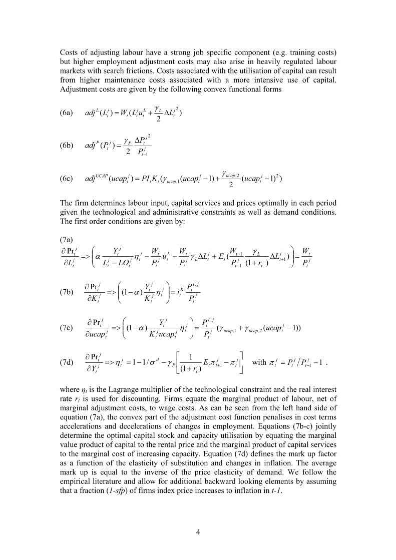
Costs of adjusting labour have a strong job specific component (e.g. training costs) but higher employment adjustment costs may also arise in heavily regulated labour markets with search frictions. Costs associated with the utilisation of capital can result from higher maintenance costs associated with a more intensive use of capital. Adjustment costs are given by the following convex functional forms

(6a) )2

()( 2jt

LLt

jtt

jt

L LuLWLadj Δ+=γ

(6b) jt

jtPj

tP

PPPadj

1

2

2)(

−

Δ=γ

(6c) ))1(2

)1(()( 22,1, −+−= j

tucapj

tucapttj

tUCAP ucapucapKPIucapadj

γγ

The firm determines labour input, capital services and prices optimally in each period given the technological and administrative constraints as well as demand conditions. The first order conditions are given by: (7a)

jt

tjt

t

Lj

t

tt

jtLj

t

tLtj

t

tjtj

tjt

jt

jt

jt

PW

LrP

WEL

PW

uPW

LOLY

L=⎟⎟

⎠

⎞⎜⎜⎝

⎛Δ

++Δ−−

−=>

∂∂

++

+ ))1(

(Pr

11

1 γγηα

(7b) jt

jItK

tj

tjt

jt

jt

jt

PP

iKY

K

,

)1(Pr

=⎟⎟⎠

⎞⎜⎜⎝

⎛−=>

∂∂

ηα

(7c) ))1(()1(Pr

2,1,

,

−+=⎟⎟⎠

⎞⎜⎜⎝

⎛−=>

∂∂ j

tucapucapjt

jItj

tjt

jt

jt

jt

jt ucap

PP

ucapKY

ucapγγηα

(7d) ⎥⎦

⎤⎢⎣

⎡−

+−−==>

∂∂

+j

tj

ttt

Pdj

tjt

jt E

rYππγση 1)1(

1/11Pr

with 11 −= −j

tj

tj

t PPπ .

where ηt is the Lagrange multiplier of the technological constraint and the real interest rate rt is used for discounting. Firms equate the marginal product of labour, net of marginal adjustment costs, to wage costs. As can be seen from the left hand side of equation (7a), the convex part of the adjustment cost function penalises in cost terms accelerations and decelerations of changes in employment. Equations (7b-c) jointly determine the optimal capital stock and capacity utilisation by equating the marginal value product of capital to the rental price and the marginal product of capital services to the marginal cost of increasing capacity. Equation (7d) defines the mark up factor as a function of the elasticity of substitution and changes in inflation. The average mark up is equal to the inverse of the price elasticity of demand. We follow the empirical literature and allow for additional backward looking elements by assuming that a fraction (1-sfp) of firms index price increases to inflation in t-1.

4

Finally we also allow for a mark up shock. This leads to the following specification of the aggregate price mark-up (7d’) [ ] P

tttttPd

t usfpsfpE −−−+−−= −+ πππβγση ))1((/11 11 10 ≤≤ sfp 1.2.2 Investment goods producers There is a perfectly competitive investment goods production sector which combines domestic and foreign final goods, using the same CES aggregators as households and governments do to produce investment goods for the domestic economy. Denote the CES aggregate of domestic and foreign inputs used by the investment goods sector with , then real output of the investment goods sector is produced by the following linear production function,

inptI

(8) I

tinptt UII =

where is a technology shock to the investment good production technology which itself follows a random walk with drift

ItU

(9) UI

tIt

UIIt ugu ε++= −1

Given our assumption concerning the input used in the investment goods production sector, investment goods prices are given by (10) . I

tC

tI

t UPP /= 1.2 Households: The household sector consists of a continuum of households . A share

of these households are not liquidity-constrained and indexed by . They have full access to financial markets, they buy and sell domestic

and foreign assets (government bonds and equity). The remaining households are liquidity-constrained and indexed by

[ 1,0∈h ])1( slc−

[ )slci −∈ 1,0

[ ]1,1 slck −∈ . These households do not trade on asset markets and consume their disposable income each period. Both types of households supply differentiated labour services to unions which maximise a joint utility function for each type of labour i. It is assumed that types of labour are distributed equally over the two household. Nominal rigidity in wage setting is introduced by assuming that the household faces adjustment costs for changing wages. These adjustment costs are borne by the household.

5

1.2.1 Non Liquidity constrained households Households decide about four types of assets, domestic and foreign nominal bonds ( ), the stock of physical capital ( ) and cash balances ( ).The household receives income from labour, nominal bonds and rental income from lending capital to firms plus profit income from firms owned by the household. Income from labour is taxed at rate t

Fit

it BB , i

tK itM

w, rental income at rate ti. In addition households pay lump-sum taxes TLS. We assume that income from financial wealth is subject to different types of risk. Domestic bonds yield risk-free nominal return equal to it. Foreign bonds are subject to an external financial intermediation premium risk(.), which is a positive function of the economy wide level of foreign indebtedness. An equity premium on real assets arises because of uncertainty about the return of real assets. The Lagrangian of this maximisation problem is given by

Ktrp

(11)

( )it

it

it

t

tt

t

iLSt

n

j

jiti

t

it

t

itwi

tt

it

wt

t

tI

tKt

t

it

IKt

KK

t

iFtt

Bt

tt

FttF

ti

t

itt

i

t

it

t

iFtt

t

it

t

iti

tt

Iti

tt

Ct

ct

tt

t

it

it

tI

KJK

TWW

PLL

PWt

PKPt

PKPrpit

P

BEuYPBEriskit

PBit

PM

PBE

PB

PMI

PPC

PPt

LCUVMax

ttt

F

t

t

10

0

0

,

1

,

1

211

1

,1

11

11

111,

0

000

)1(

Pr2

)1(

))(1())(1)()1(1(

))1(1()1(

)1,(

11

−

∞

=

∞

=

=−

−−

−−

−−

−−

−−−

∞

=

−−−Ε−

⎟⎟⎟⎟⎟⎟⎟⎟⎟⎟⎟

⎠

⎞

⎜⎜⎜⎜⎜⎜⎜⎜⎜⎜⎜

⎝

⎛

+−Δ

+−

−

+−−

−−−−+

−

−+−−++++

+

Ε−

−Ε=

∑

∑

∑

∑

−−

δβξ

γδ

βλ

β

The utility function is non-separable in consumption ( ) and leisure ( ) of the King, Plosser, Rebelo (1988) type. We also allow for habit persistence in consumption and leisure. Thus temporal utility for consumption is given by

itC i

tL−1

(12) ( ) ( )( )[ ]ρ

ωεερκ

−−−−−

=−−

−−

11)exp(1)exp()1,(

1

11 tLi

tLtt

Cit

Cti

tit

LhLChCLCU

The investment decisions w. r. t. real capital are subject to convex adjustment costs, therefore we make a distinction between real investment expenditure (I) and physical investment (J). Investment expenditure of households including adjustment costs is given by

(13) 2)(22

1 it

Iit

itKi

tit J

KJJI Δ+⎟

⎟⎠

⎞⎜⎜⎝

⎛⎟⎟⎠

⎞⎜⎜⎝

⎛+=

γγ

6

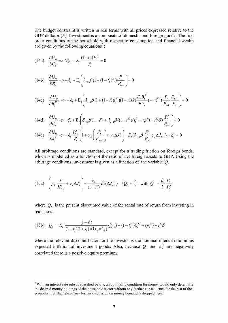
The budget constraint is written in real terms with all prices expressed relative to the GDP deflator (P). Investment is a composite of domestic and foreign goods. The first order conditions of the household with respect to consumption and financial wealth are given by the following equations2:

(14a) 0)1(,

0 =+

−=>∂∂

t

Ct

ct

ti

tCit P

PtUCU λ

(14b) 0))1(1(1

10 =⎟⎟

⎠

⎞⎜⎜⎝

⎛−+Ε+−=>

∂∂

++

t

tt

itttti

t PP

itBU

βλλ

(14c) 0))(1)()1(1( 1

11,

0 =⎟⎟⎠

⎞⎜⎜⎝

⎛−−−+Ε+−=>

∂∂ +

++

t

t

t

tBt

tt

FttF

tittttiF

t EE

PP

uYPBE

riskitBU F

βλλ

(14d) 0)))(1(()1(1

110 =⎟⎟

⎠

⎞⎜⎜⎝

⎛+−−+−Ε+−=>

∂∂

+++

t

ItK

tit

Kt

Kttttti

t PPtrpit

KU δβλδβξξ

(14e) 0)(1 11

11

10 =+Δ−⎟⎟⎠

⎞⎜⎜⎝

⎛Δ+⎟⎟

⎠

⎞⎜⎜⎝

⎛+−=>

∂∂

++

+−

−t

itI

t

It

ttitIi

t

it

Kt

It

tit

JPPEJ

KJ

PP

JU ξγβλγγλ

All arbitrage conditions are standard, except for a trading friction on foreign bonds, which is modelled as a function of the ratio of net foreign assets to GDP. Using the arbitrage conditions, investment is given as a function of the variable tQ

(15a) ( 1)()1( 1

1

−=Δ+

−⎟⎟⎠

⎞⎜⎜⎝

⎛Δ+ +

−t

itt

t

IitIi

t

it

K QJEr

JKJ γγγ ) with I

t

t

t

tt P

PQ

λξ

=

where is the present discounted value of the rental rate of return from investing in real assets

tQ

(15b) δπ

δ Kt

Kt

Kt

KttI

tttit

tt trpitQit

EQ +−−+++−

−= +

+

))(1())1/()1)(1(

)1(( 11

where the relevant discount factor for the investor is the nominal interest rate minus expected inflation of investment goods. Also, because and are negatively correlated there is a positive equity premium.

tQ Itπ

2 With an interest rate rule as specified below, an optimality condition for money would only determine the desired money holdings of the household sector without any further consequence for the rest of the economy. For that reason any further discussion on money demand is dropped here.

7

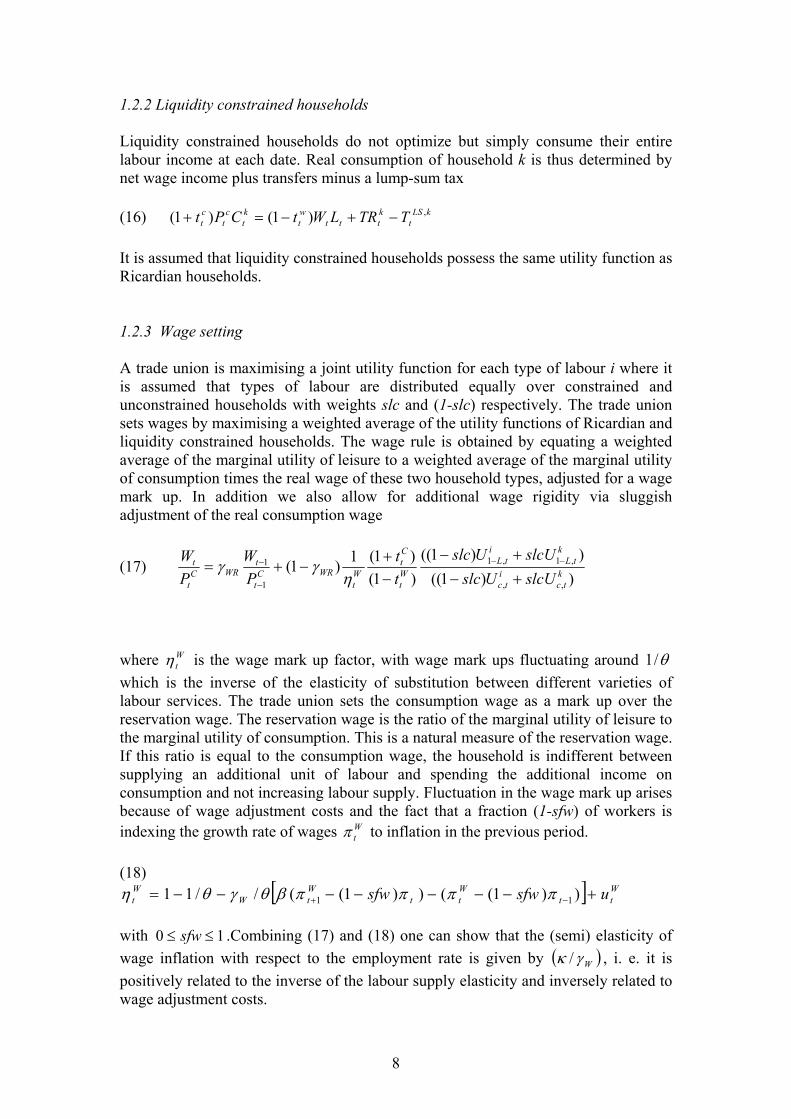
1.2.2 Liquidity constrained households Liquidity constrained households do not optimize but simply consume their entire labour income at each date. Real consumption of household k is thus determined by net wage income plus transfers minus a lump-sum tax (16) kLS

tkttt

wt

kt

ct

ct TTRLWtCPt ,)1()1( −+−=+

It is assumed that liquidity constrained households possess the same utility function as Ricardian households. 1.2.3 Wage setting A trade union is maximising a joint utility function for each type of labour i where it is assumed that types of labour are distributed equally over constrained and unconstrained households with weights slc and (1-slc) respectively. The trade union sets wages by maximising a weighted average of the utility functions of Ricardian and liquidity constrained households. The wage rule is obtained by equating a weighted average of the marginal utility of leisure to a weighted average of the marginal utility of consumption times the real wage of these two household types, adjusted for a wage mark up. In addition we also allow for additional wage rigidity via sluggish adjustment of the real consumption wage

(17) ))1((

))1(()1()1(1)1(

,,

,1,1

1

1k

tci

tc

ktL

itL

Wt

Ct

Wt

WRCt

tWRC

t

t

slcUUslcslcUUslc

tt

PW

PW

+−+−

−+

−+= −−

−

−

ηγγ

where is the wage mark up factor, with wage mark ups fluctuating around W

tη θ/1 which is the inverse of the elasticity of substitution between different varieties of labour services. The trade union sets the consumption wage as a mark up over the reservation wage. The reservation wage is the ratio of the marginal utility of leisure to the marginal utility of consumption. This is a natural measure of the reservation wage. If this ratio is equal to the consumption wage, the household is indifferent between supplying an additional unit of labour and spending the additional income on consumption and not increasing labour supply. Fluctuation in the wage mark up arises because of wage adjustment costs and the fact that a fraction (1-sfw) of workers is indexing the growth rate of wages to inflation in the previous period. W

tπ (18)

[ ] Wtt

Wtt

WtW

Wt usfwsfw +−−−−−−−= −+ ))1(())1((//11 11 ππππβθγθη

with .Combining (17) and (18) one can show that the (semi) elasticity of wage inflation with respect to the employment rate is given by

10 ≤≤ sfw( )Wγκ / , i. e. it is

positively related to the inverse of the labour supply elasticity and inversely related to wage adjustment costs.

8

1.2.4 Aggregation The aggregate of any household specific variable in per capita terms is given by

since households within each group are identical.

Hence aggregate consumption is given by

htX

∫ +−==1

0)1( k

tit

htt slcXXslcdhXX

(19a) k

titt slcCCslcC +−= )1(

and aggregate employment is given by (19b) with . k

titt slcLLslcL +−= )1( t

kt

it LLL ==

Since liquidity constrained households do not own financial assets we have

. 0=== kt

Fkt

kt KBB

1.3 Trade and the current account So far we have only determined aggregate consumption, investment and government purchases but not the allocation of expenditure over domestic and foreign goods. In order to facilitate aggregation we assume that households, the government and the corporate sector have identical preferences across goods used for private consumption, public expenditure and investment. Let { }iGiGiii ICICZ ,, ,,,∈ be the demand of an individual household, investor or the government, then their preferences are given by the following utility function

(20a) )1(1111

)()1(−−−

⎥⎥⎦

⎤

⎢⎢⎣

⎡++−−=

M

M

M

M

MM

M

M ifMt

MidMt

Mi ZusZusZσσ

σσ

σσσ

σ

where the share parameter sM can be subject to random shocks and idZ and ifZ are indexes of demand across the continuum of differentiated goods produced respectively in the domestic economy and abroad, given by.

(20b) 1

1

11

1−

=

−

⎥⎥

⎦

⎤

⎢⎢

⎣

⎡⎟⎠⎞

⎜⎝⎛= ∑

d

d

d

ddn

h

idh

id Zn

Zσσ

σσ

σ ,

1

1

11

1−

=

−

⎥⎥

⎦

⎤

⎢⎢

⎣

⎡⎟⎠⎞

⎜⎝⎛= ∑

f

f

f

ffm

h

ifh

if Zm

Zσσ

σσ

σ

9

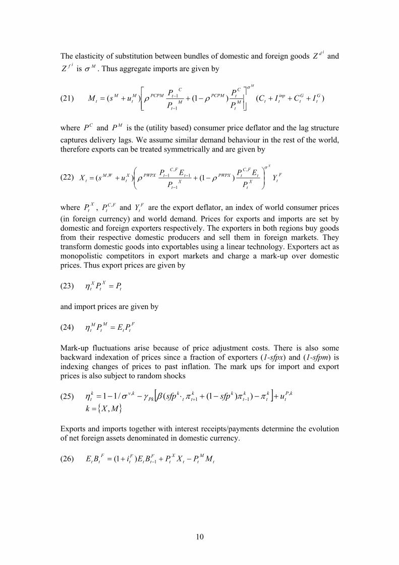
The elasticity of substitution between bundles of domestic and foreign goods idZ and ifZ is . Thus aggregate imports are given by Mσ

(21) )()1()(1

1 Gt

Gt

inpttM

t

CtPCPM

Mt

CtPCPMM

tM

t ICICPP

PP

usM

M

+++⎥⎥⎦

⎤

⎢⎢⎣

⎡−++=

−

−

σ

ρρ

where and is the (utility based) consumer price deflator and the lag structure captures delivery lags. We assume similar demand behaviour in the rest of the world, therefore exports can be treated symmetrically and are given by

CP MP

(22) FtX

t

tFC

tPWPXX

t

tFC

tPWPXXt

WMt Y

PEP

PEP

usX

Xσ

ρρ ⎟⎟⎠

⎞⎜⎜⎝

⎛−++=

−

−−,

1

1,

1, )1()(

where , and are the export deflator, an index of world consumer prices (in foreign currency) and world demand. Prices for exports and imports are set by domestic and foreign exporters respectively. The exporters in both regions buy goods from their respective domestic producers and sell them in foreign markets. They transform domestic goods into exportables using a linear technology. Exporters act as monopolistic competitors in export markets and charge a mark-up over domestic prices. Thus export prices are given by

XtP FC

tP , FtY

(23) t

Xt

Xt PP =η

and import prices are given by (24) F

ttM

tMt PEP =η

Mark-up fluctuations arise because of price adjustment costs. There is also some backward indexation of prices since a fraction of exporters (1-sfpx) and (1-sfpm) is indexing changes of prices to past inflation. The mark ups for import and export prices is also subject to random shocks (25) [ ] kP

tkt

kt

kktt

kPk

kvkt usfpsfp ,

11, ))1((/11 +−−+⋅−−= −+ πππβγση

{ }MXk ,= Exports and imports together with interest receipts/payments determine the evolution of net foreign assets denominated in domestic currency. (26) t

Mtt

Xt

Ftt

Ft

Ftt MPXPBEiBE −++= −1)1(

10

1.4 Policy We assume that fiscal and monetary policy is partly rules based and partly discretionary. Policy responds to an output gap indicator of the business cycle. The output gap is not calculated as the difference between actual and efficient output but we try to use a measure that closely approximates the standard practice of output gap calculation as used for fiscal surveillance and monetary policy (see Denis et al. (2006)). Often a production function framework is used where the output gap is defined as deviation of capital and labour utilisation from their long run trends. Therefore we define the output gap as

(27) αα

⎟⎟⎠

⎞⎜⎜⎝

⎛⎟⎟⎠

⎞⎜⎜⎝

⎛=

−

sst

tsst

tt L

LucapucapYGAP

)1(

.

where and are moving average steady state employment rate and capacity utilisation:

sstL ss

tucap

(28) j

tucapss

tucapss

t ucapucapucap ρρ +−= −1)1( (29) t

Lsssst

Lsssst LLL ρρ +−= −1)1(

which we restrict to move slowly in response to actual values. 1.4.1 Fiscal Policy Both expenditure and receipts are responding to business cycle conditions. On the expenditure side we identify the systematic response of government consumption, government transfers and government investment to the business cycle. For government consumption and government investment we specify the following rules

(30) CGt

iit

CGit

CGAdj

Gt

CGLag

GCGLag

Gt uygapcgycgyccc ++−+Δ+Δ−=Δ ∑ −−− ττττ )()1( 11

(31) IGt

iit

IGit

IGAdj

Gt

IGLag

GIGLag

Gt uygapigyigyiii ++−+Δ+Δ−=Δ ∑ −−− ττττ )()1( 11

Government consumption and government investment can temporarily deviate from their long run targets cgy and igy (expressed as ratios to GDP in nominal terms) in response to fluctuations of the output gap. Due to information and implementation lags the response may occur with some delay. This feature is captured by a distributed lag of the output gap in the reaction function. The transfer system provides income for unemployed and for pensioners and acts as an automatic stabiliser. The generosity of the social benefit system is characterised by three parameters: the fraction of the non-employed which receive unemployment benefits and the level of payments for unemployed and pensioners. In other words the number of non-participants is treated as a government decision variable. NPARTPOP

11

We assume that unemployment benefits and pensions are indexed to wages with replacement rates and respectively and we formulate the following linear transfer rule

Ub Rb

(32) . TR

tP

ttR

tNPART

tW

ttU

t uPOPWbLPOPPOPWbTR ++−−= )( Government revenues are financed by taxes on consumption as well as capital and labour income.

GtR

(33) 1−++= t

It

Kt

Ktt

ct

cttt

wt

Gt KPitCPtLWtR

Following the OECD estimates for revenue elasticities (van den Noord (2000)) we assume that consumption and capital income tax follow a linear scheme, and a progressive labour income tax schedule

(34a) TWtt

wwt UYt

w1

0τ

τ= where measures the average tax rate, and the degree of progressivity. A simple first-order Taylor expansion around a zero output gap yields

w0τ

w1τ

(34b) t

wwwwt ygapt 100 τττ +=

Government debt ( ) evolves according to tB (35) . t

LSt

Gtt

Gt

Ct

Gt

Ctttt TRTRIPCPBiB −−++++= −1)1(

There is a lump-sum tax ( ) used for controlling the debt to GDP ratio according to the following rule

LStT

(36) ⎟⎟⎠

⎞⎜⎜⎝

⎛Δ+−=Δ

−−

−

tt

tDEFT

tt

tBLSt PY

Bb

PYB

T ττ )(11

1

where is the government debt target. Tb 1.4.2 Central bank policy rule (interest rate rule) Monetary policy is modelled via the following Taylor rule, which allows for some smoothness of the interest rate response to the inflation and output gap (37)

INOMttt

INOMy

tINOMy

TCt

INOMTEQINOMlagt

INOMlagt

uygapygap

ygaprii

+−+

+−++−+=

−

−−

)(

])()[1(

12,

11,1

τ

τππτπττ π

12

The central bank has a constant inflation target and it adjusts interest rates whenever actual consumer price inflation deviates from the target and it also responds to the output gap. There is also some inertia in nominal interest rate setting.

Tπ

2. Estimation Our technological assumptions imply that domestic and foreign GDP and its components are stationary in growth rates. Our model implies that various nominal ratios such as the consumption to GDP ratio (cyn), the investment to GDP ratio (iyn), the government consumption to GDP ratio (cgyn), the government investment to GDP ratio (igyn), the government transfers to wages ratio (trw), the trade balance3 share in GDP (tbyn), the wage share (ws), the employment rate (L) and the real exchange rate (RER) are stationary. Concerning nominal variables we assume that the domestic and foreign inflation target is a constant. This implies that domestic wage inflation rate ( ), domestic and foreign price inflation (wπ π , ) rates and nominal domestic and foreign interest rates ( i , ) are stationary, as well as certain price ratios, in particular the relative import (P

FπFi

P

M/P) and export price (PXP

/P) ratios. These variables, together with the exogenous technology shock to the investment good production ( ) form our information set. World economy series [ , , Δy

IUFi Fπ F] are considered as

exogenous and are modeled as a VAR(1) process. To assure stationarity of the Y/YW ratio, an equilibrium correction term is added to the ΔyF equation. This introduces a small feedback of domestic demand into world demand. The model is estimated on quarterly data for the euro area over the period 1981Q1 to 2006Q1, taken from the ECB AWM data base and updated with Eurostat quarterly national accounts database. Some data transformations are taken:

1. all real quantities are divided by the (linear) trend of active population, to obtain per-capita data;

2. relative linear trends in price indexes and real quantities have been removed, except for the trend in wage share, which is not removed from the data;

3. the trend in the series of employment is also removed; 4. the pension component of the transfer rule is removed from the data prior to

estimation: this eliminates the trend in the transfer to wage share and only the reaction coefficient is estimated. Ub

All the exogenous observed processes (world economy, technology shock to investment good production) have been estimated separately to the rest of the model parameters. The parameters listed in Table 1 are calibrated and kept constant over the estimation exercise. The reaction of wage taxes to output gap is set to 0.8, following OECD estimates.

Wt1

3 Concerning the import and export share we remove a trade integration trend prior to estimation. As import and export data for the euro area include intra euro-area trade we also assumed the foreign demand and price terms in the export (22) and import price equation (24) were a weighted average of foreign and domestic terms, with a share of 0.5 of intra euro area trade in total trade.

13

TABLE 1. Calibrated parameters

Structural parameters Steady states α 0.52 cgy 0.203

Gα 0.9 igy 0.025 β 0.996 UIg 0

δ 0.025 π , Fπ 0.005 Gδ 0.0125 popWg 0.00113

τB 4.e-6 Yg , YFg 0.003

τDEF 4.e-3 UPg 0.0024

bT 2.4 ucap 1 dσ 10 L 0.65 INOMρ 0 XWX ωω = EXρ , IMρ 0.975 θ 1.6 LOLρ 0.99 TRWS 0.36

Kt , , ct w0τ 0.2

w1τ 0.8

Other parameters are determined according to steady state constraints:

• )1/KSN-(1*)-(1 1, ατγ =ucap , determined in order to assure the steady state constraint ucap = 1, where PPIYKKSN /*/= is the nominal capital to GDP share.

• ω is determined in order to assure the steady state condition 65.0=L The dynamical forms of government spending and government investment have been identified by estimating separately from the rest of the model an array of models of the general form: (38)

ttkmm

nkkktm

m

nt eu

LaLaLbLbLb

uLaLa

LbLbLbg

nn

+−−−

+++++

−−−

+++=Δ

++++

,1

,1,0,,1

1

,11,10,1

...1...

......1

...11 δδδδδδ

where is the growth rate of the government spending or government investment, L is the lagged operator and are the inputs. The selection of the model is then

taken considering both the

tgΔ

tiu ,

2TR statistics, based on the response error, and information criteria. For both government consumption and investment, the input is the output gap plus an error correction to assure stationarity of the nominal shares to GDP. This implied a two step-procedure, where first the dynamical structure was identified using a HP-

14

filtered output gap. The obtained structure and coefficients are fed into the DSGE model, which is estimated given the previously identified coefficients. At this stage, we obtain a model based output gap which is again fed into the separated identification procedure to check the validity of the structure identified with HP-filtered output gap. The coefficients in the government spending rules are then estimated together with the other parameters in the DSGE model. Thus, the estimated government consumption rule takes the form (30) CG

ttCG

tCGAdj

Gt

CGLag

GCGLag

Gt uygapcgycgyccc +Δ+−+Δ+Δ−=Δ −− 111 )()1( ττττ

(31) IG

ttIG

tIGAdj

Gt

IGLag

GIGLag

Gt uygapigyigyiii +Δ+−+Δ+Δ−=Δ −− 111 )()1( ττττ

The model parameters are estimated applying the Bayesian approach as, e.g., Schorfheide (2000), Smets and Wouters (2003). From the computational point of view, the DYNARE toolbox for MATLAB has been applied (Juillard, 1996-2005). 2.1 Prior distributions Exogenous AR shocks have beta distributions for auto-correlation coefficients with prior mean at 0.85 except for the monetary shock, where we set prior mean to 0.5 (i.e. we did not have any ‘preference’ between a persistent shock or a white noise) and for the overhead labour shock, where we set prior mean to 0.95. Standard errors have prior gamma distributions, with prior mean values at

• 0.5% for ‘persistent shocks’ (accounting for different trends in the data, like overhead labour,) and for shocks to risk premia;

• 0.25% for monetary shock; • 5% for technology shock, preference and adjustment costs shocks, nominal

GDP shares of government consumption, investment, transfers; • 10% for mark-up shocks

For the fiscal parameters, we set a prior around zero for τCG and τIG, to let the data drive pro-cyclical or counter-cyclical reaction of government consumption and investment to changes in the output gap. For transfers we also set a neutral prior mean of bU at 0. Persistence in the government spending rule has a prior at 0.5, while for investment and transfers this is set to 0.85. For price and wage rigidities we roughly follow Smets and Wouters (2003), but allowing a wider variation in the upper bound (prior mean at 30). Capital and labour adjustment costs have similar priors, while for investment the prior is smaller (15). Prior consumption and leisure habits are set at 0.7. Inverse of intertemporal elasticities have prior gamma distributions with mean 1.25 and standard deviation 0.5 (2 and 1 for ). The share of liquidity constrained households has a neutral prior at 0.5, with standard deviation 0.1, similar to Forni et al. (2006). Finally, the share of forward looking behaviour in hybrid Phillips curves and the price indexation coefficients in import and export equations have prior mean at 0.5 in the range [0, 1].

Cσ

15

2.2 Posterior estimation The draws from the posterior distribution have been obtained by taking two parallel chains of 300,000 runs of Metropolis. Convergence of the Markov Chain has been tested by cumulated means and by the diagnostics by Brooks and Gelman (1998). The shape of the likelihood at the posterior mode and the Hessian condition number have been also considered to highlight lack of identification for some parameters4. In Table 2.1 we show prior distributions and posterior estimations of our structural parameters (see Table A1 in the annex for estimates of standard errors of shocks and AR coefficients of autocorrelated shocks and Figure A1 for the plots of priors and posterior distributions). The estimated fraction of forward looking price setting behaviour is high. The posterior mean for sfp is estimated at 0.87, which implies only 13 percent of firms keep prices fixed at the t-1 level. The estimated share of liquidity-constrained consumers is 0.35, which is similar to estimates reported in Coenen and Straub (2005) and lower than in Forni et al. (2006). Note that our estimates also suggest a degree of habit persistence in consumption of 0.56 and an intertemporal elasticity of substitution of around 0.25.

4 Only for two structural parameters does the likelihood not dominate the prior, namely for export price rigidity ( PXγ ) and risk. See also Canova and Sala (2005) about identification problems in the Smets and Wouters model and in DSGE models in general.

16

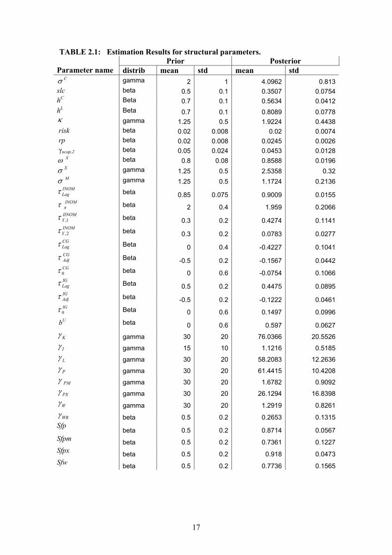
TABLE 2.1: Estimation Results for structural parameters. Prior Posterior

Parameter name distrib mean std mean std Cσ gamma 2 1 4.0962 0.813

slc beta 0.5 0.1 0.3507 0.0754hC Beta 0.7 0.1 0.5634 0.0412hL Beta 0.7 0.1 0.8089 0.0778κ gamma 1.25 0.5 1.9224 0.4438 risk beta 0.02 0.008 0.02 0.0074 rp beta 0.02 0.008 0.0245 0.0026 γucap,2 beta 0.05 0.024 0.0453 0.0128

Xω beta 0.8 0.08 0.8588 0.0196Xσ gamma 1.25 0.5 2.5358 0.32Mσ gamma 1.25 0.5 1.1724 0.2136

INOMLagτ beta 0.85 0.075 0.9009 0.0155

INOMπτ beta 2 0.4 1.959 0.2066IINOMY 1,τ beta 0.3 0.2 0.4274 0.1141INOMY 2,τ beta 0.3 0.2 0.0783 0.0277CGLagτ Beta 0 0.4 -0.4227 0.1041CGAdjτ Beta -0.5 0.2 -0.1567 0.0442CG0τ beta 0 0.6 -0.0754 0.1066IGLagτ Beta 0.5 0.2 0.4475 0.0895IGAdjτ beta -0.5 0.2 -0.1222 0.0461IG0τ Beta 0 0.6 0.1497 0.0996

bU beta 0 0.6 0.597 0.0627

Kγ gamma 30 20 76.0366 20.5526

Iγ gamma 15 10 1.1216 0.5185

Lγ gamma 30 20 58.2083 12.2636

Pγ gamma 30 20 61.4415 10.4208

PMγ gamma 30 20 1.6782 0.9092

PXγ gamma 30 20 26.1294 16.8398

Wγ gamma 30 20 1.2919 0.8261

WRγ beta 0.5 0.2 0.2653 0.1315Sfp

beta 0.5 0.2 0.8714 0.0567Sfpm beta 0.5 0.2 0.7361 0.1227Sfpx beta 0.5 0.2 0.918 0.0473Sfw beta 0.5 0.2 0.7736 0.1565

17

The estimated fiscal response parameters are counter-cyclical for government transfers. We find a positive response of transfers to the employment gap bU (=0.6). Government consumption responds negatively to the current change in the output gap. The investment rule appears procyclical, with a high degree of persistence. The only parameter relevant for stabilisation policy on the revenues side is the degree of progressivity of wage taxes. Due to a lack of reliable data on tax rates we do not estimate this parameter but set it corresponding to the OECD estimate of the elasticity of tax revenues with respect to the output gap5. By way of comparison, other studies that have analysed the actual behaviour of fiscal authorities have mainly focused on the overall deficit rather than on government expenditure catagories seperately. Gali and Perotti (2003) assess the extent to which the constraints associated with the Maastricht Treaty and the Stability and Growth pact have made fiscal policy in EMU countries more procyclical. They find discretionary fiscal policy (as measured by the primary cyclically adjusted deficit of general government) was procyclical in EMU countries before Maastricht and essentially acyclical after Maastricht. They also find an increase in the degree in counter-cyclicality of non-discretionary fiscal policy (as measured by the difference between the total primary deficit and the cyclically-adjusted primary deficit) in EMU countries. In contrast, von Hagen and Wyplosz (2007), using data until 2006, find that the primary cyclically adjusted deficit has become countercyclical after 1992 and was acyclical before. European Commission (2004, Ch.3) also find evidence of a change in the response of the total primary budget balance to the output gap, with an insignificant impact of the cycle on primary balances before 1994 and a significant positive impact of the output gap on the primary balance post 1994. Concerning transfers, our results are consistent with those of Darby and Melitz (2007), who find that age- and health-related social expenditure as well as incapacity benefits all react to the cycle in a stabilising manner. In Figure 1 we show the one step ahead predictions of the model for the growth rates of GDP ( ), consumption ( ), investment ( ), labour ( ), government consumption ( ), government investment ( ), government transfers ( ), as well as for inflations (

Yg Cg Ig LgGg GIg TRg

π , , ), wage inflation ( ), growth rate of investment specific technological progress ( ), nominal interest rates ( , ), nominal

exchange rate ( ), world inflation ( ), world GDP ( ).

Mπ Xπ WπUIg i Fi

Eg Fπ YWgWe also show the fit of nominal ratios to GDP of consumption (cyn), government consumption (cgyn), government investment (igyn), investment (iyn), trade balance (tbyn), transfers to wages ratio (trw), the real foreign GDP to domestic GDP ratio (ywy) as well as the stationary real exchange rate (ER), labour (L), wage share (ws), import to GDP deflator (PM/P), export to GDP deflator (PX/P).

5 The OECD calculates an elasticity of income tax revenue with respect to the output gap of 1.5 and an elasticity of the wage bill w.r.t. the gap of 0.7. This implies an elasticity of the tax rate w.r.t. to output gap of 0.8.

18

FIGURE 1. In-sample one step ahead predictions of the estimated model. (Data are grey lines; model predictions are black lines)

1980 1990 2000-0.01

0

0.01

0.02gY

t

1980 1990 2000-0.02

0

0.02gC

t

1980 1990 2000-0.05

0

0.05gI

t

1980 1990 2000

-50

5

x 10-3 gLt

1980 1990 2000-0.02

0

0.02

gGCt

1980 1990 2000-0.02

0

0.02

gGIt

1980 1990 2000-0.02

0

0.02

gTRt

1980 1990 2000

0

0.02

0.04πt

1980 1990 2000-0.05

0

0.05

πtM

1980 1990 2000-0.02

0

0.02

0.04

πtX

1980 1990 2000-0.02

0

0.02

0.04

πWt

1980 1990 2000-0.01

0

0.01gt

UI

1980 1990 20000

0.05inomt

1980 1990 20000

0.05inomt

F

1980 1990 2000-0.1

0

0.1gE

t

1980 1990 20000

0.01

0.02

πtF

1980 1990 2000-0.01

0

0.010.02

gYFt

1980 1990 2000

-0.56

-0.54

log(CSNt)

19

1980 1990 2000-0.2

0

0.2

log(ERt)

1980 1990 2000-0.02

0

0.02

0.04TBYNt

1980 1990 2000-1.64

-1.6

-1.56log(GSNt)

1980 1990 2000-3.8

-3.6

log(GISNt)

1980 1990 2000-1.8

-1.7

-1.6

log(ISNt)

1980 1990 2000

-0.45

-0.4log(Lt)

1980 1990 2000

0.5

0.6

WSt

1980 1990 2000-0.2

0

0.2log(PMt/Pt)

1980 1990 2000-0.1

0

0.1log(PXt/Pt)

1980 1990 20000.34

0.36

0.38

0.4TRSNt

1980 1990 2000-0.05

0

0.05log(YWYt)

20

2.3 Model comparisons A quite widely applied method to assess the validity of the estimated DSGE models is to compare them with non-structural linear reduced-form models such as VARs or BVARs (see e.g. Sims, 2003; Schorfheide, 2004; Smets and Woutyers, 2003; Juillard et al. 2006). In Table 2.2 we compare our base model with BVAR models (lags 1 to 12) using Sims and Zha (1998) priors. The BVAR estimates were obtained following Juillard et al. (2006), combining the Minnesota prior with dummy observations. The prior decay and tightness parameters are set to 0.5 and 3, respectively. As in Juillard et al. (2006), the parameter determining the weight on own-persistence (sum-of-coefficients on own lags) is set at 2 and the parameter determining the degree of co-persistence is set at 5. To obtain priors for error terms we used the residuals from unconstrained AR(1) processes estimated over a sample of observations that was extended back to 1978Q1 (the DSGE model is estimated over a sample starting from 1981Q1). The marginal data density of the DSGE has been obtained from the two-chain, 300,000 replications of the Metropolis-Hastings Algorithm using the modified harmonic mean formula suggested by Geweke. Similarly to other estimated DSGE’s in the literature, our base model has a better marginal likelihood than BVAR’s. Although the robustness of these kinds of results is sometimes criticized, for the reason that it may depend on different prior assumptions in both the DSGE and the BVAR, BVARs are a potentially useful metric for comparing the out-of-sample performance of DSGE models. TABLE 2.2. Comparison of the fit of the base model and of BVAR’s.

Marginal likelihood BVAR(1) 6752.695 BVAR(2) 6835.592 BVAR(3) 6831.757 BVAR(4) 6835.782 BVAR(5) 6836.935 BVAR(6) 6828.311 BVAR(7) 6837.512 BVAR(8) 6835.597 BVAR(9) 6835.392 BVAR(10) 6827.01 BVAR(11) 6825.155 BVAR(12) 6829.694

DSGE model 7066.91

21

In Table 2.3 we also report the RSME’s of the 1-step and 4-step ahead predictions of the DSGE model and of a VAR(1) that includes error corrections mimicking the long run restrictions implied by the model concerning nominal ratios. In Figure 1 bis we also show the plots of the 1-step ahead fit of the VAR(1). The in-sample RMSE’s of the VAR(1) are obviously better than those of the DSGE, and they are useful to have an idea of the ‘upper’ bound of the in-sample fit. This does not obviously imply a better performance of the VAR out-of-sample (see above discussion on BVAR comparison). It is interesting to note that for most of the observed variables, the DSGE performs better in the 4-step than in the 1-step ahead prediction horizons.

TABLE 2.3. Comparison of the fit of the base model and a VAR(1) with error error corrections reproducing long run constraints of the DSGE model. RMSE’s are reported for 1-step and 4-step ahead predictions.

DSGE 1-step

VAR(1) 1-step

DSGE 4-step

VAR(1) 4-step

Ytg 0.005581 0.003838 0.005459 0.00482

Ctg 0.005357 0.00349 0.00501 0.004114

Itg 0.015205 0.010913 0.014945 0.013367

Gtg 0.00462 0.0037 0.00443 0.004028

IGtg 0.005466 0.003365 0.011552 0.00761

TRtg 0.005454 0.002583 0.005077 0.00341

Ltg 0.001489 0.001214 0.002099 0.001488

Wtπ 0.007895 0.004743 0.007112 0.00552

tinom 0.001156 0.00086 0.002804 0.00162

tπ 0.003208 0.002401 0.003706 0.00290

Mtπ 0.012617 0.009285 0.014677 0.01213

Xtπ 0.006065 0.004675 0.00728 0.00582

Etg 0.02927 0.020961 0.027276 0.024352

22

23

2.4 Variance decompositions In Tables 2.4-6 we report the posterior intervals of the variance decomposition for conditional variance (1-step and 4-step ahead) and unconditional variance. The short run variation of GDP growth is mainly driven by shocks to productivity, the private demand components, in particular investment, and trade. Monetary and fiscal policy shocks play a relatively small role and explain a portion in the range of 5-13% of the short term variation. Price and wage mark up shocks play an even smaller role. The long run decomposition of GDP growth does not change strongly, except for a slightly larger role of the wage mark up shock and productivity and a smaller contribution of investment. Notice, these results are difficult to compare with variance decompositions from other models, since we are looking at GDP growth, instead of GDP levels. Inflation in the short run is mainly driven by shocks to the price mark up, while the long run variation is dominated by shocks to the wage mark up. Monetary policy shocks play a negligible role in the variation of inflation both in the short and the long run. This is in line with decomposition presented by Smets et al. (2007). The variance of the growth rate of the nominal exchange rate is largely driven by trade and risk premium shocks both in the short and the long run. There is a small role for both domestic and foreign monetary policy shocks. The short run variation in the nominal consumption share is driven by various shocks (trade, investment, own consumption shock, as well as risk premium and productivity shocks) while the productivity shock plays a more dominant role for the 4-step ahead conditional variance. The investment share is mainly driven by its own shock and the productivity shock. Unconditional variances of the nominal shares are dominated by the productivity shock. The trade balance ratio is mainly driven by trade and risk premium shocks, while the wage mark-up shock plays an important role in explaining the variance in employment and the wage share.

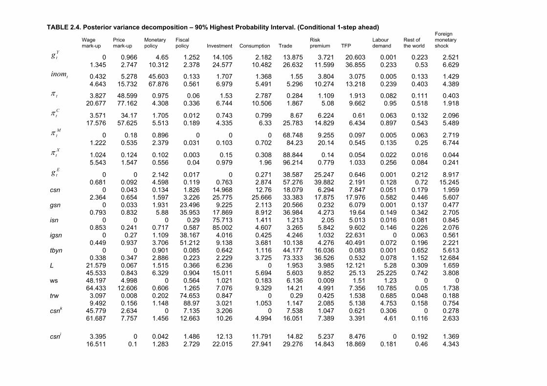
TABLE 2.4. Posterior variance decomposition – 90% Highest Probability Interval. (Conditional 1-step ahead)

Wage mark-up

Price mark-up

Monetary policy

Fiscal policy Investment Consumption Trade

Risk premium TFP

Labour demand

Rest of the world

Foreign monetary shock

Ytg 0 0.966 4.65 1.252 14.105 2.182 13.875 3.721 20.603 0.001 0.223 2.521

1.345 2.747 10.312 2.378 24.577 10.482 26.632 11.599 36.855 0.233 0.53 6.629

tinom 0.432 5.278 45.603 0.133 1.707 1.368 1.55 3.804 3.075 0.005 0.133 1.429 4.643 15.732 67.876 0.561 6.979 5.491 5.296 10.274 13.218 0.239 0.403 4.389

tπ 3.827 48.599 0.975 0.06 1.53 2.787 0.284 1.109 1.913 0.082 0.111 0.403 20.677 77.162 4.308 0.336 6.744 10.506 1.867 5.08 9.662 0.95 0.518 1.918

Ctπ 3.571 34.17 1.705 0.012 0.743 0.799 8.67 6.224 0.61 0.063 0.132 2.096

17.576 57.625 5.513 0.189 4.335 6.33 25.783 14.829 6.434 0.897 0.543 5.489 Mtπ 0 0.18 0.896 0 0 0 68.748 9.255 0.097 0.005 0.063 2.719

1.222 0.535 2.379 0.031 0.103 0.702 84.23 20.14 0.545 0.135 0.25 6.744 Xtπ 1.024 0.124 0.102 0.003 0.15 0.308 88.844 0.14 0.054 0.022 0.016 0.044

5.543 1.547 0.556 0.04 0.979 1.96 96.214 0.779 1.033 0.256 0.084 0.241 Etg 0 0 2.142 0.017 0 0.271 38.587 25.247 0.646 0.001 0.212 8.917

0.681 0.092 4.598 0.119 0.763 2.874 57.276 39.882 2.191 0.128 0.72 15.245 csn 0 0.043 0.134 1.826 14.968 12.76 18.079 6.294 7.847 0.051 0.179 1.959 2.364 0.654 1.597 3.226 25.775 25.666 33.383 17.875 17.976 0.582 0.446 5.607 gsn 0 0.033 1.931 23.496 9.225 2.113 20.566 0.232 6.079 0.001 0.137 0.477 0.793 0.832 5.88 35.953 17.869 8.912 36.984 4.273 19.64 0.149 0.342 2.705 isn 0 0 0 0.29 75.713 1.411 1.213 2.05 5.013 0.016 0.081 0.845 0.853 0.241 0.717 0.587 85.002 4.607 3.265 5.842 9.602 0.146 0.226 2.076 igsn 0 0.27 1.109 38.167 4.016 0.425 4.246 1.032 22.631 0 0.063 0.561 0.449 0.937 3.706 51.212 9.138 3.681 10.138 4.276 40.491 0.072 0.196 2.221 tbyn 0 0 0.901 0.085 0.642 1.116 44.177 16.036 0.083 0.001 0.652 5.613 0.338 0.347 2.886 0.223 2.229 3.725 73.333 36.526 0.532 0.078 1.152 12.684 L 21.579 0.067 1.515 0.366 6.236 0 1.953 3.985 12.121 5.28 0.309 1.659 45.533 0.843 6.329 0.904 15.011 5.694 5.603 9.852 25.13 25.225 0.742 3.808 ws 48.197 4.998 0 0.564 1.021 0.183 6.136 0.009 1.51 1.23 0 0 64.433 12.606 0.606 1.265 7.076 9.329 14.21 4.991 7.356 10.785 0.05 1.738 trw 3.097 0.008 0.202 74.653 0.847 0 0.29 0.425 1.538 0.685 0.048 0.188 9.492 0.156 1.148 88.97 3.021 1.053 1.147 2.085 5.138 4.753 0.158 0.754 csnk 45.779 2.634 0 7.135 3.206 0 7.538 1.047 0.621 0.306 0 0.278 61.687 7.757 1.456 12.663 10.26 4.994 16.051 7.389 3.391 4.61 0.116 2.633

csni 3.395 0 0.042 1.486 12.13 11.791 14.82 5.237 8.476 0 0.192 1.369 16.511 0.1 1.283 2.729 22.015 27.941 29.276 14.843 18.869 0.181 0.46 4.343

TABLE 2.5. Posterior variance decomposition – 90% Highest Probability Interval. (Conditional 4-step ahead)

Wage mark-up

Price mark-up

Monetary policy

Fiscal policy Investment Consumption Trade

Risk premium TFP

Labour demand

Rest of the world

Foreign monetary shock

Ytg 0.573 0.791 3.989 1.233 11.317 1.969 16.297 4.078 24.331 0.059 0.313 2.249

3.456 2.297 8.86 2.439 20.285 9.452 28.698 10.332 41.259 0.419 0.664 5.14

tinom 2.299 2.085 11.408 0.322 5.87 8.309 2.789 10.828 2.895 0.031 0.669 3.673 18.312 9.625 26.407 0.787 15.265 20.109 10.1 21.801 12.391 0.728 1.587 8.304

tπ 12.938 19.846 1.823 0.052 2.119 6.043 0.697 2.039 1.909 0.219 0.234 0.608 43.949 45.58 6.288 0.457 10.044 19.083 3.278 7.909 11.466 2.039 0.94 2.783

Ctπ 10.347 15.697 2.096 0.029 1.754 3.821 5.893 6.232 0.841 0.181 0.226 1.829

37.18 34.37 6.671 0.337 8.174 14.525 20.164 14.819 8.903 1.82 0.93 4.991 Mtπ 0.418 0.212 0.837 0.003 0.064 0.174 68.001 9.48 0.117 0.018 0.194 2.457

3.095 0.724 2.309 0.032 0.391 0.873 83.211 19.887 0.733 0.247 0.479 6.31 Xtπ 3.09 0.222 0.244 0.006 0.284 0.805 76.307 0.312 0.109 0.057 0.031 0.087

13.409 1.921 1.201 0.089 2.107 4.647 91.057 1.691 2.204 0.629 0.174 0.48 Etg 0.013 0.018 2.244 0.02 0.039 0.342 37.883 24.073 0.656 0.002 0.276 9.046

0.724 0.168 4.703 0.12 0.835 2.908 56.28 38.621 2.181 0.13 0.788 15.385 csn 0.003 0.011 0.088 0.865 12.445 19.81 6.602 8.716 14.58 0.052 0.412 2.173 2.984 0.211 0.817 1.843 24.593 37.484 13.859 19.559 28.388 0.795 0.961 4.491 gsn 0.092 0.273 1.734 17.113 7.506 2.047 11.323 0.325 21.707 0.012 0.283 0.49 3.5 1.123 5.232 30.961 16.112 11.066 24.777 3.065 39.201 0.421 0.687 1.766 isn 0.001 0 0.001 0.176 66.502 2.281 0.771 2.449 6.737 0.021 0.203 0.962 1.162 0.183 0.273 0.477 80.88 8.617 2.03 7.513 15.264 0.224 0.509 2.293 igsn 0.025 0.038 0.152 78.792 0.497 0.034 0.294 0.189 6.678 0.001 0.018 0.067 0.517 0.224 0.856 90.025 2.073 0.981 0.909 0.923 15.324 0.043 0.093 0.412 tbyn 0.01 0.003 0.93 0.126 1.105 3.608 23.475 30.158 0.265 0.003 2.229 9.295 0.837 0.119 2.472 0.37 4.228 9.317 40.287 50.312 0.773 0.093 3.213 13.586 L 38.021 0.128 1.087 0.281 5.169 0.001 1.606 3.627 7.943 2.374 0.349 1.349 66.582 0.941 5.311 0.787 14.072 5.574 4.387 9.24 19.422 9.483 0.845 3.188 ws 63.646 1.407 0.125 0.099 0.228 3.877 0.846 0.118 0.806 1.757 0.004 0.042 83.758 4.429 1.143 0.29 1.783 15.08 2.346 2.051 3.788 12.747 0.061 0.466 trw 18.638 0.057 0.534 30.644 2.706 0.001 0.763 1.95 4.302 1.148 0.203 0.681 40.738 0.53 2.966 57.057 8.248 3.122 2.471 5.831 11.843 5.504 0.545 1.863 csnk 72.439 0.548 0.047 1.848 0.779 0.634 1.067 0.719 0.368 0.173 0.003 0.098 86.666 2.255 0.357 4.939 4.095 6.975 2.759 3.99 3.023 4.799 0.135 0.993 csni 6.455 0 0.067 0.731 10.318 14.873 4.802 7.466 13.487 0.001 0.378 1.623 25.02 0.082 0.768 1.554 21.369 32.976 11.461 16.996 25.968 0.18 0.87 3.661

25

TABLE 2.6. Posterior variance decomposition – 90% Highest Probability Interval. (Unconditional variance)

Wage mark-up

Price mark-up

Monetary policy

Fiscal policy Investment Consumption Trade

Risk premium TFP

Labour demand

Rest of the world

Foreign monetary shock

Ytg 1.959 0.811 4.017 1.215 10.692 2.284 15.606 4.097 24.094 0.075 0.375 2.693

5.595 2.347 8.745 2.37 19.044 10.292 27.371 10.282 40.416 0.528 0.745 5.542

tinom 12.237 0.339 1.545 0.236 4.011 9.181 2.477 7.865 5.35 0.087 0.355 1.331 41.207 1.514 3.808 0.948 20.184 34.775 6.814 18.296 17.481 1.318 1.155 4.039

tπ 25.437 9.128 1.08 0.066 1.531 3.697 0.718 2.321 2.593 0.336 0.129 0.349 60.978 22.619 4.379 0.355 11.451 19.403 3.236 7.696 16.839 3.644 0.586 1.665

Ctπ 23.333 7.158 1.042 0.053 1.411 3.423 3.156 4.054 2.109 0.312 0.112 0.834

57.303 17.748 4.454 0.314 11.078 18.272 10.584 10.799 15.644 3.459 0.562 2.783 Mtπ 3.152 0.204 0.809 0.021 0.365 0.951 58.345 7.859 0.438 0.051 0.211 2.272

12.386 0.655 2.136 0.093 2.826 4.418 75.868 17.296 3.193 0.732 0.46 5.673 Xtπ 7.938 0.173 0.337 0.018 0.565 1.125 52.166 0.856 0.737 0.155 0.049 0.126

29.026 1.318 1.503 0.125 5.322 8.741 75.642 3.326 7.432 1.812 0.213 0.56 Etg 0.527 0.023 2.136 0.033 0.268 0.946 36.767 23.047 0.937 0.007 0.5 9.345

2.86 0.191 4.478 0.145 1.645 3.847 54.777 37.199 2.561 0.212 1.005 15.48 csn 0.41 0.006 0.014 0.085 3.814 1.726 0.641 1.236 60.317 0.087 0.031 0.138 8.179 0.031 0.107 0.491 20.661 10.162 2.647 6.681 83.618 0.706 0.217 0.768 gsn 3.878 0.142 0.762 12.681 4.431 1.603 5.727 0.257 32.794 0.152 0.129 0.239 16.231 0.616 2.784 26.87 11.245 7.434 15.604 1.571 53.367 1.415 0.411 0.923 isn 0.423 0.002 0.007 0.028 7.682 0.237 0.102 0.134 56.755 0.054 0.011 0.049 8.799 0.029 0.076 0.346 30.473 5.829 0.788 2.342 84.711 0.585 0.103 0.368 igsn 0.036 0.004 0.016 90.311 0.089 0.009 0.034 0.02 1.151 0.001 0.002 0.011 0.898 0.052 0.201 98.44 0.623 0.304 0.267 0.23 7.327 0.055 0.027 0.115 tbyn 0.709 0.002 0.413 0.102 0.786 3.452 18.037 35.407 0.277 0.001 1.944 6.04 5.843 0.065 1.234 0.508 4.834 13.513 32.705 60.979 1.019 0.083 2.942 9.509 L 41.385 0.01 0.013 0.013 0.487 0.01 0.069 0.206 6.033 2.066 0.009 0.028 87.536 0.101 0.431 0.119 7.752 0.685 0.52 1.601 37.96 14.695 0.076 0.228 ws 17.045 0.214 0.133 0.018 0.12 1.567 0.201 0.128 0.223 23.587 0.011 0.051 63.013 1.058 0.923 0.076 0.656 6.893 0.638 0.712 1.053 72.265 0.083 0.256 trw 39.387 0.01 0.013 0.2 0.48 0.021 0.068 0.19 5.986 1.627 0.007 0.027 86.046 0.099 0.419 3.75 7.622 0.664 0.514 1.521 36.937 14.032 0.072 0.22 csnk 59.105 0.084 0.072 0.312 0.217 0.591 0.171 0.118 3.104 3.975 0.004 0.022 85.889 0.446 0.456 1.375 2.609 3.019 0.539 0.911 12.521 25.205 0.033 0.16 csni 2.467 0.007 0.029 0.084 3.758 1.575 0.553 0.91 52.13 0.071 0.032 0.105 23.495 0.048 0.179 0.425 19.421 8.743 2.283 5.982 80.318 1.42 0.195 0.632

26

3. Impulse Response Analysis We now proceed to investigate the effects of various structural shocks on the euro area economy. We use the estimated DSGE model to analyse the impulse responses of the main economic variables to structural shocks and the uncertainty surrounding these effects. The magnitude of the shocks is given by the posterior estimate of one standard deviation of the shock, i.e. we used the full joint posterior distribution of structural parameters and shocks to produce the Bayesian uncertainty bounds of the IRFs. Figures 2 to 4 show the response for the estimated model to a government consumption, investment and transfers shock respectively. The government consumption and investment shocks raise government spending as a share of output, but spending gradually returns to baseline. An increase in government consumption raises GDP temporarily, however it crowds out the interest sensitive demand components such as private investment and consumption of Ricardian households, while consumption of liquidity constrained households rises because of higher wage income. However, in the medium run liquidity constrained consumers also cut back consumption spending because of an increase in lump sum taxes, needed to finance the government spending shock. Notice, however, the aggregate consumption multiplier of government consumption is negative. This result seems at first sight in conflict with the findings of Gali et al. (2007). They show that allowing for a fraction of credit constrained consumers exceeding 25%, a model with sticky prices can account for a positive consumption response to a government spending shock. However, their model assumes no nominal wage rigidities and no labour adjustment costs (in our notation γw = γL = 0). In contrast our estimation results show that especially the labour adjustment cost parameter Lγ is significantly different from zero. A sensitivity analysis (see annex) shows that when these parameters tend to zero (as assumed in Gali et al (2007)), the consumption response to a government spending shocks tends to become positive in our model too. The economic interpretation of this result is simple. Negligible wage and labour adjustment costs imply a stronger positive short run impact of an increase in government consumption on labour income and therefore a stronger response of private consumption. Our results can also be compared to Coenen and Straub (2005). They estimate a DSGE model for the euro area similar to Smets and Wouters (2003), but introduce non-Ricardian households in the model similar to our liquidity constrained consumers. For a lower share of non-Ricardian households (between 0.25 and 0.37) they find a short-lived rise in liquidity- constrained consumption, but falling below its steady state level already after a few quarters, caused by a rise in lump-sum taxes due to the build up of government debt. Forni et al. (2006) find a positive response of consumption to both a government purchases and a government employment shock, but assume no fiscal response to cyclical conditions and no labour adjustment costs To assess the impact of the government spending shocks on output in terms of traditional "multipliers", the impact effect for a 1 percent of government spending shock on GDP is 0.73 in the first quarter, falling to 0.45 in the fourth. It remains positive for seven to eight years, and then turns negative. Cumulated over the first year the multiplier is 0.56. This is somewhat smaller than results reported in Roeger and in ’t Veld (2004) for the QUEST II model, which shows multipliers for the largest

27

four European countries between 0.85 and 0.956. The estimated impact fiscal multiplier is within the range found in empirical studies of fiscal policy using structural vector autoregression (SVAR) models. Blanchard and Perotti (2002) applied SVAR methodology to study the effects of fiscal policy in the US and various authors have extended the SVAR methodology to include other countries. Perotti (2005) finds large differences in the effects of fiscal policy, with the responses of GDP and consumption having become weaker over time. Only for the US is the consumption response found positive and did the GDP multiplier exceed 1 in the post 1980 period. The effect of government investment on GDP is more favourable (see figure 3), because government investment has a positive supply effect. Because of this the effect is also less inflationary and therefore requires a smaller interest rate response of the central bank. However one should notice that the government investment multiplier hinges importantly on the output elasticity of public capital which is not estimated. The parameter is calibrated such as to obtain a marginal product of public capital equal to the marginal product of private capital in the steady state. Figure 4 shows the responses to a government transfer shock. The increase in transfers raises disposable incomes and boosts liquidity-constrained consumption Ck

directly. There is a negative impact on consumption of non liquidity-constrained consumers, but this is much smaller and aggregate consumption is positively affected by the transfer shock. Again, fiscal policy crowds out private investment. Figure 5 presents the level comparison of the estimated effect of an orthogonalised shock to nominal interest rates ( ). The shock leads to a rise in the (annualised) nominal short-term interest rate of 0.4 percentage points on impact. The real short-term interest rate increases by more. The monetary policy shock is not very persistent and nominal interest rates return quickly to base. The shock leads to a hump-shaped fall in output. The maximum effect on investment is about three times as large as that on consumption and the peak effects occur after about two quarters. Inflation also peaks in the second quarter

INOMtε

7 but we do not see the hump-shaped response in consumer price inflation that is a persuasive feature of many estimated VARs. This could be due to our small open economy assumption where we do not allow the Euro exchange rate to affect export prices of the rest of the world. This implies that the appreciation of the Euro is immediately passed on to domestic consumer prices. In a more realistic multi country setting the inflation response would likely be more delayed. Real wages fall in response to the monetary policy shock and employment is also negatively affected. Fiscal spending falls but the decline is less than that of GDP as fiscal policy acts counter-cyclically and partly offsets to effects of the monetary contraction.

6 There the government consumption shock is a weighted average of government purchases and wage expenditures. Wage expenditure shocks have larger effects on GDP than government purchases shocks. 7 Lack of inflation inertia and inflation persistence has been a feature of many DSGE models. Cogley and Sbordone (2005) show that allowing for a shifting trend in the inflation target can improve the empirical description of the inflation process.

28

FIGURE 2. Response to a government consumption shock. Yt Ct It

0 20 40-5

0

5

10x 10

-4

0 20 40-6

-4

-2

0x 10

-4

0x 10

-4

-2

-4

-60 20 40

TBYNtCit Ck

t

0 20 40-10

-5

0

5x 10

-4

0 20 40-2

0

2

4x 10

-4

2x 10

-4

0

-20 20 40

Gt GIt TRt

0 20 40-5

0

5

10x 10

-3

0 20 40-5

0

5

10x 10

-4

5x 10

-4

0

-5

-100 20 40

0 20 400

1

2

3

4x 10-4 Lt

0 20 40-4

-2

0

2

4x 10-4 WRt

0 20 40-2

-1

0

1

2x 10-3 deficitt

0 20 40-5

0

5

10x 10-4 log(YGAPt)

0 20 40-2

0

2

4x 10-4 πt

0 20 400

0.5

1

1.5x 10-4 πc

t

0 20 400

0.5

1

1.5x 10-4 inomt

0 20 40-2

0

2

4x 10-4 Rt

0 20 40-1

0

1

2x 10-3 et

29

FIGURE 3. Response to a government investment shock. Yt Ct It

0 20 400

0.5

1x 10

-3

0 20 400

2

4

6

8x 10

-4

5x 10

-4

0

-5

-100 20 40

TBYNtCit Ck

t

0 20 40-5

0

5

10x 10

-4

0 20 400

0.5

1x 10

-3

2x 10

-4

0

-20 20 40

Gt GIt TRt

0 20 40-5

0

5

10x 10

-4

0 20 400

0.02

0.04 10x 10

-4

5

0

-50 20 40

0 20 40-2

0

2

4x 10-4 Lt

0 20 400

0.5

1x 10-3 WRt

0 20 40-5

0

5

10x 10-4 deficitt

0 20 40-5

0

5

10x 10-4 log(YGAPt)

0 20 40-2

0

2x 10-4 πt

0 20 40-2

0

2x 10-4 πc

t

0 20 40-2

0

2

4x 10-4 inomt

0 20 40-2

0

2x 10-4 Rt

0 20 40-1

0

1

2x 10-3 et

30

FIGURE 4. Response to a government transfers shock. Yt Ct It

0 20 40-2

0

2

4x 10

-4

0 20 40-5

0

5

10x 10

-4

1x 10

-4

0

-1

-2

-30 20 40

TBYNtCit Ck

t

0 20 40-4

-2

0

2x 10

-4

0 20 40-2

0

2

4x 10

-3

5x 10

-5

0

-5

-100 20 40

Gt GIt TRt

0 20 40-2

0

2

4x 10

-4

0 20 40-2

0

2

4x 10

-4

10x 10

-3

5

0

-50 20 40

0 20 40-5

0

5

10x 10-5 Lt

0 20 40-2

0

2

4x 10-4 WRt

0 20 40-5

0

5

10

15x 10-4 deficitt

0 20 40-2

0

2

4x 10-4 log(YGAPt)

0 20 40-5

0

5

10x 10-5 πt

0 20 40-5

0

5

10x 10-5 πc

t

0 20 400

2

4

6x 10-5 inomt

0 20 40-5

0

5x 10-5 Rt

0 20 40-5

0

5

10x 10-4 et

31

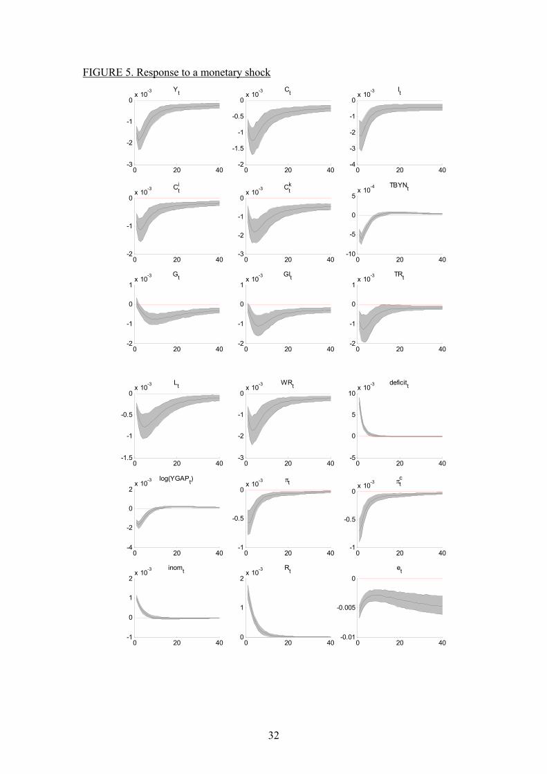
FIGURE 5. Response to a monetary shockYt Ct It

0 20 40-3

-2

-1

0x 10

-3

0 20 40-2

-1.5

-1

-0.5

0x 10

-3

0x 10

-3

-1

-2

-3

-40 20 40

TBYNtCit Ck

t

0 20 40-2

-1

0x 10

-3

0 20 40-3

-2

-1

0x 10

-3

5x 10

-4

0

-5

-100 20 40

Gt GIt TRt

0 20 40-2

-1

0

1x 10

-3

0 20 40-2

-1

0

1x 10

-3

1x 10

-3

0

-1

-20 20 40

0 20 40-1.5

-1

-0.5

0x 10-3 Lt

0 20 40-3

-2

-1

0x 10-3 WRt

0 20 40-5

0

5

10x 10-3 deficitt

0 20 40-4

-2

0

2x 10-3 log(YGAPt)

0 20 40-1

-0.5

0x 10-3 πt

0 20 40-1

-0.5

0x 10-3 πc

t

0 20 40-1

0

1

2x 10-3 inomt

0 20 400

1

2x 10-3 Rt

0 20 40-0.01

-0.005

0et

32

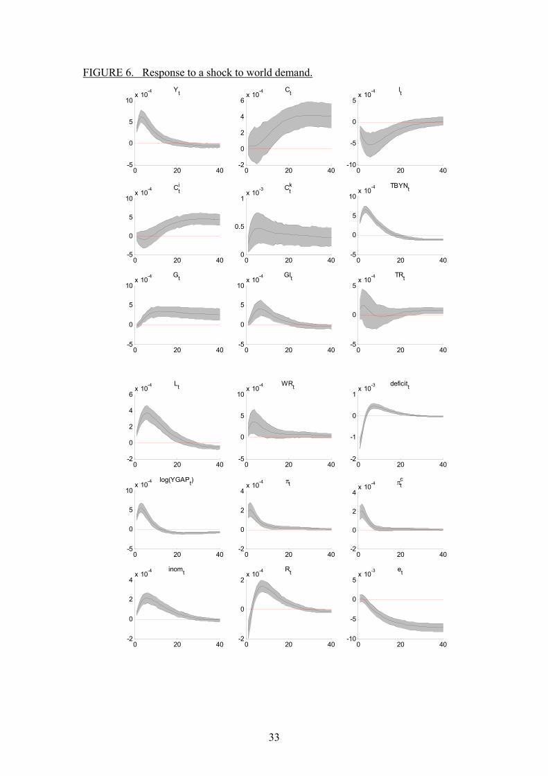
FIGURE 6. Response to a shock to world demand. Yt Ct It

0 20 40-5

0

5

10x 10

-4

0 20 40-2

0

2

4

6x 10

-4

5x 10

-4

0

-5

-100 20 40

TBYNtCit Ck

t

0 20 40-5

0

5

10x 10

-4

0 20 400

0.5

1x 10

-3

10x 10

-4

5

0

-50 20 40

Gt GIt TRt

0 20 40-5

0

5

10x 10

-4

0 20 40-5

0

5

10x 10

-4

5x 10

-4

0

-50 20 40

0 20 40-2

0

2

4

6x 10-4 Lt

0 20 40-5

0

5

10x 10-4 WRt

0 20 40-2

-1

0

1x 10-3 deficitt

0 20 40-5

0

5

10x 10-4 log(YGAPt)

0 20 40-2

0

2

4x 10-4 πt

0 20 40-2

0

2

4x 10-4 πc

t

0 20 40-2

0

2

4x 10-4 inomt

0 20 40-2

0

2x 10-4 Rt

0 20 40-10

-5

0

5x 10-3 et

33

FIGURE 7. Response to a shock to TFP. Yt Ct It

0 20 400

0.005

0.01

0 20 400

0.005

0.01

0.015

0 20 400

1

2

3

4x 10

-3

TBYNtCit Ck

t

0 20 400

0.005

0.01

0.015

0 20 400

0.005

0.01

0.015 4x 10

-4

2

0

-20 20 40

Gt GIt TRt

0 20 40-5

0

5

10x 10

-3

0 20 40-5

0

5

10x 10

-3

0.015

0 20

0.01

0.005

040

0 20 40-3

-2

-1

0x 10-3 Lt

0 20 400

0.005

0.01

0.015WRt

0 20 40-10

-5

0

5x 10-3 deficitt

0 20 40-4

-2

0

2x 10-3 log(YGAPt)

0 20 40-2

-1

0

1x 10-3 πt

0 20 40-10

-5

0

5x 10-4 πc

t

0 20 40-10

-5

0

5x 10-4 inomt

0 20 40-5

0

5

10x 10-4 Rt

0 20 40-10

-5

0

5x 10-3 et

34

Our last example of a demand shock is a shock to foreign demand. Figure 6 presents the level comparison of the estimated effect of an orthogonalised shock to world output ( ). Because of nominal rigidities an increase in world demand leads first to an increase in capacity utilisation and employment. The initial excess demand is only gradually reduced by an increase in domestic prices. In the long run there is a positive output effect resulting from the terms of trade effect induced by a permanent shift in world demand for domestic goods. Government expenditure increases in line with nominal GDP (government purchases and investment) and the wage sum (government transfers), but they increase by less than would be the case if there was no active fiscal policy as the output and employment gap are positive. Thus fiscal policy limits the increase in aggregate demand and stabilises output. The overall effect of fiscal stabilisation is to reduce the initial increase in employment. Automatic stabilisation via transfers also smoothes consumption of liquidity-constrained households C

YFtε

k . Figure 7 presents the level comparison of the estimated effect of an orthogonalised shock to TFP ( ). Because TFP follows a random walk, the productivity shock results in a permanent increase of output, consumption and investment. The real wage also rises, but there is a rather persistent negative employment effect. It is well known (see Gali, 1999) that with nominal rigidities supply shocks lead to a demand externality. Because firms lower prices insufficiently as a response to a cost-reducing shock, there is a lack of aggregate demand which makes it optimal for individual firms to lower employment. Expansionary government consumption partially compensates for the shortfall in demand. The automatic stabilisation via government transfers work in the same direction, since they respond to the decline in employment and boost consumption of liquidity constrained households.

Ytε

4 Medium term trends: the case of a declining wage share

A continuously declining wage share over the sample period is an important stylised fact for the European economy. In our empirical analysis we allow for two mechanisms which allow the model to match this fact, namely a declining share of overhead labour and a secular increase in the mark up of prices over marginal cost. Unfortunately both shocks are not directly observable; however, they can be identified by using the model because they affect first order conditions differently. The overhead labour shock only affects the labour demand equation while the mark up shock affects labour demand and investment in a similar fashion. Both explanations have some empirical validity. It is likely that structural reforms in the goods market and in particular large scale privatisations which occurred in various euro area member states over the sample period may have lead to a decline in overhead labour. It is also likely that the economy-wide mark up has increased over the sample period due to an increasing share of services in total output. As documented in many sectorial studies on mark ups (see for example Oliveira Martins et al., 1997) the service sector tends to have higher mark ups (the absence of both shocks in the US case is also consistent with a relatively stable US wage share). In the following we use the model in a counterfactual analysis in order to first determine the relative importance of the two explanations in accounting for the evolution of the wage share and second for explaining the economic consequences of these trends.

35

As can be seen from Figures 8 and 9, our estimates indicate that the share of overhead labour in total employment LOL has fallen by about 20% points and mark ups have increased by about 5% points. As shown in figure 10, the decline in overhead labour explains about 50% of the decline in the wage share. Both effects explain a large fraction of the decline (60-70%). The reduction in overhead labour increases productivity without increasing the marginal product of production workers (marginal productivity of labour actually falls), this leads to a decline in the wage share. Because firms can supply the same output with less labour and the marginal product of labour has declined, the reduction in overhead labour does not by itself lead to an increase in factor demand. In fact it reduces the demand for labour since the reduction of fixed costs reduces the marginal product of labour. Therefore there is a new equilibrium with less labour input, lower GDP, lower real wages but higher average productivity. The increase in the price mark up affects the measured mark up directly and leads to a reduction of both factor inputs. In contrast to a reduction in overhead labour the mark up shock reduces labour and capital inputs simultaneously. Finally, we can ask the question whether both shocks acted independently or whether there is a correlation between them. Theoretically it is plausible that a reduction in overhead labour could have removed entry barriers and thus have led to a reduction in mark ups, suggesting a positive correlation, i.e. corr(lol,eta) > 0. Alternatively it is also possible that an increase in the mark up could have increased overhead labour via some rent sharing agreements between workers and firms, implying a negative correlation, i.e. corr(lol,eta) < 0 , and therefore restrict the decline in LOL. A small negative correlation (corr(lol,eta) = -0.22) can be observed in the reconstruction of the historical shocks (smoothed shocks).

36

FIGURE 8. Counterfactual experiment: solid lines are for the case when the level of LOL remains fixed at the values of begin of 80’s; dashed lines show the actual data.

Yt Ct It0.4

1960 1980 2000 20200

0.2

0.4

1960 1980 2000 20200

0.2

0.4

1960 1980 2000 2020-0.2

0

0.2

Lt TBt/Yt WSt0.1 0.04 0.8

1960 1980 2000 2020-0.1

0

1960 1980 2000 2020-0.02

0

0.02

1960 1980 2000 20200.4

0.6

E_LOLWt/Pt RERt 0.4

1960 1980 2000 20200

0.2

0.4

1960 1980 2000 2020-0.5

0

0.5

1960 1980 2000 20200

0.1

0.2

0.3

37

FIGURE 9. Counterfactual experiment: solid lines are for the case when the level of mark-up shocks remains fixed at the values of begin of 80’s; dashed lines show the actual data.

Yt Ct It0.6

1960 1980 2000 20200

0.2

0.4

1960 1980 2000 20200

0.2

0.4

1960 1980 2000 2020-0.2

0

0.2

0.4

Lt TBt/Yt WSt0.1 0.04 0.8

1960 1980 2000 2020-0.1

0

1960 1980 2000 2020-0.02

0

0.02

1960 1980 2000 20200.4

0.6

ηtWt/Pt RERt 1.05

1960 1980 2000 20200

0.1

0.2

0.3

1960 1980 2000 2020-0.2

0

0.2

0.4

1960 1980 2000 20200.85

0.9

0.95

1

38

FIGURE 10. Counterfactual experiment: upper plots show the actual wage share, the decline of the actual wage share which is explained by the decrease in labour overhead and in price mark-up. The bottom plot compares the actual wage share data with the two counterfactual experiments.

1980 1990 20000.45

0.5

0.55

0.6

0.65Wage share

1980 1990 2000-0.08

-0.06

-0.04

-0.02

0WS-WSLOL

1980 1990 2000-0.02

-0.015

-0.01

-0.005

0WS-WSη

1975 1980 1985 1990 1995 2000 2005 20100.46

0.48

0.5

0.52

0.54

0.56

0.58

0.6

0.62wage share

original dataLOL counterfactualETA counterfactual

39

5 Conclusions In this paper we have described the estimation of an open economy DSGE model for the euro area. So far most estimated DSGE models have mainly been concerned with monetary policy analysis. We have extended the model by incorporating fiscal reaction functions that allow the model to be used for fiscal policy analysis. Fiscal policy is effective in the model as we allow for financial market rigidities that force some households to consume their current wage and transfer income. Our paper differs also from other estimated DSGE models in that it treats the euro area as an open economy and is not estimated using detrended data, which allows us to analyse the effects of non stationary productivity shocks. In future research we intent to extend this analysis in various directions. It would be interesting to explore how the stabilising properties of the estimated rules compare to simple optimal rules. We have also disregarded automatic stabilisation from other revenue components. This requires a more careful analysis of various tax rules. In future research, more attention will also have to be devoted to fiscal stabilisation at the level of euro area member states. 6 References Adolfson, M., Laseén, S., Lindé, J. Villani, M., 2007. Forecasting Performance of an

Open Economy DSGE Model. Econometric Reviews 26, 289-328. Artis, M.J., Onorante, L., 2006. The economic importance of fiscal rules. CEPR

Discussion Paper no. 5684. Blanchard, O., Perotti, R., 2002. An Empirical Characterization of the Dynamic

Effects of Changes in Government Spending and Taxes on Output. Quarterly Journal of Economics 117 (4), 1329-68.

Brooks, S. , Gelman, A., 1998. General methods for monitoring convergence of iterative simulations. Journal of Computational and Graphical Statistics 7, 434- 456.

Canova, F. , Sala, L., 2005. Back to square one: identification issues in DSGE models. IGIER Working Paper 303

Coenen, G., Straub, R., 2005. Does government spending crowd in private consumption? Theory and empirical evidence from the euro area. International Finance 8(3), 435-470.

Darby, J., Melitz, J., 2007. Labour Market Adjustment, Social Spending and Automatic Stabilizers in the OECD. CEPR Discussion Paper no. 6230.

Denis, C. , Mc Morrow, K., Roeger, W., 2002. Production function approach to calculating potential growth and output gaps – Estimates for the EU member states and the US. European Economy Economic Papers No. 176.

European Commission, 2004. Public Finances in EMU 2004, European Economy. Fatas, A., Mihov, I., 2003. The case for restricting fiscal policy discretion. The

Quarterly Journal of Economics 118 (4), 1419-47. Forni, L., Monteforte, L., Sessa, L., 2006. The estimated general equilibrium effects

of fiscal policy: the case of the euro area, mimeo. Gali, J, Gertler, L., Lopez-Salido, J., 2001. European Inflation Dynamics, European

Economic review 45(7), 1121-50.

40

Gali, J., Perotti, R., 2003. Fiscal Policy in EMU, Economic Policy 37, 553-72. Gali, J, Lopez-Salido, J., Valles, J., 2007. Understanding the Effects of Government

Spending on Consumption. Journal of the European Economic Association 5 (1), 227-270.

Juillard, M., 1996, 2005. DYNARE Manual, Version 3.0, 2005. mimeo. Juillard, M., Kamenik, O., Kumhof, M., Laxton, D., 2007. Measures of Potential

Output from an Estimated DSGE Model of the United States. mimeo. Oliveira-Martins, J. , Scarpetta, S., Pilat, D., 1997. Mark-up Pricing, Market

Structure and the Business Cycle. OECD Economic Studies 27, Paris. Perotti, R., 2005. Estimating the Effects of Fiscal Policy in OECD countries. CEPR

Discussion Paper no. 4842. Phelps, E. , 1967. Phillips Curves, Expectations and Inflation, and optimal

Unemployment over Time. Economica 34, 254-81. Ratto, M., 2008. Analysing DSGE models with Global Sensitivity Analysis,

Computational Economics 31, 115-139. Ratto, M., Pagano A., Young, P., 2007. State Dependent Parameter metamodelling

and sensitivity analysis. Computer Physics Communications 177, 863-876. Ratto, M., Roeger, W., in ’t Veld, J., Girardi, R., 2005. An estimated new Keynesian

dynamic stochastic general equilibrium model of the Euro area, European Economy, Economic Papers No. 220. European Commission. Brussels.

Roeger, W., in ’t Veld, J., 2004. Some Selected Simulation Experiments with the European Commission’s QUEST model. Economic Modelling 21(5), 785-832.

Saltelli, A., Tarantola, S., Campolongo, F., Ratto, M., 2004. Sensitivity Analysis in Practice: A Guide to Assessing Scientific Models. John Wiley and Sons.

Schorfheide, F., 2000. Loss function-based evaluation of DSGE models. Journal of Applied Econometrics 15, 645-670.

Schorfheide, F., 2004. Notes on Model Evaluation. Department of Economics, University of Pennsylvania.

Sims, C., 2003. Matlab Procedures to Compute Marginal Data Densities for VARs with Minnesota and Training Sample Priors. Department of Economics, Princeton University.

Sims, C., Zha, T., 1998. Bayesian methods for dynamic multivariate models. International Economic Review 49, 949-968.

Smets, F., Wouters, R., 2003. An Estimated Dynamic Stochastic General Equilibrium Model of the Euro Area. Journal of the European Economic Association 1, 1123-1175.

Smets, F., Wouters, R., 2007. Shocks and Frictions in US Business Cycles: A Bayesian DSGE Approach. American Economic Review 97, 586-606.

Van den Noord, P., 2000, The Size and Role of automatic fiscal Stabilizers in the 90s and beyond. OECD Economics Department Working Paper No 303, Paris.

Von Hagen, J. and C. Wyplosz (2007), EMU's Decentralized System of Fiscal Policy. European Economy, Economic Papers No. 306. European Commission. Brussels. .

41

FIGURES FIGURE 1 bis: fit of a VAR(1) including VECM corrections matching those implied by the DSGE model.

1980 1990 2000-0.02

0

0.02gY

t

1980 1990 2000-0.02

0

0.02gC

t

1980 1990 2000-0.05

0

0.05gI

t

1980 1990 2000-0.01

0

0.01gL

t

1980 1990 2000-0.02

0

0.02

gGCt

1980 1990 2000-0.04-0.02

00.020.04

gGIt

1980 1990 2000-0.02

0

0.02gTR

t

1980 1990 2000-0.01

00.010.020.03

πt

1980 1990 2000-0.05

0

0.05πM

1980 1990 2000-0.02

0

0.02

0.04πXt

1980 1990 2000-0.02

0

0.02

0.04πWt

1980 1990 2000

-0.01

0

0.01gUI

1980 1990 2000

0

0.02

0.04inomt

1980 1990 2000

0

0.02

0.04inomF

t

1980 1990 2000-0.1

0

0.1gE

t

1980 1990 2000-0.01

00.010.02

πFt

1980 1990 2000-0.02

0

0.02gYF

t

42

ANNEX 1 The steady state The DSGE model implies a number of long run restrictions for growth rates, nominal shares and price ratios. The determination of the steady state of the model is described below, where steady state is denoted by the endogenous names without the index t. Long run growth rates and inflations are calibrated as follows:

00113.00005.0

003.0

=

=

==

POP

UI

Y

gg

gπ

The steady state of real per capita GDP growth rate determines all the real growth rates of the model, except for investment, which is given by:

UIYI ggg += . The steady state of GDP deflator inflation defines the steady state of all inflation rates in the model and also of nominal wage inflation, as:

YW g+= ππ The technology growth is determined by:

UIG

YG

UP gα

-α(-gg )21 αααα −−+

=

Nominal interest rate is given by:

1/1 −+= βπi The model allows for a generalised case, where the rate of time preference in the domestic and foreign countries is different, implying different steady state nominal interest rates. The net foreign asset share to GDP is thus given by:

riskiibynYPBE FF

t

F

/)( −==

This implies a steady state level for the nominal trade balance share:

FPOPY bynggitbyn )( +++−= π

43

By combining the GDP equilibrium condition and equations (21-24), the identity can be expressed only in terms of trade balance, real exchange

rate and foreign to domestic GDP ratio, ywy. The latter ratio is calibrated at 1, allowing to obtain ER from tbyn. From this all the price ratios can be determined as:

tbynimynexyn =− )(

( )1/

/)1(/

/

11

)1(

=

⎥⎦⎤

⎢⎣⎡ −+=

=

−−

YX

YMMMYC

YM

PP

PPssPP

ERPP

MM

X

σσ

α

where is the share of intra trade, calibrated at 0.5. The import and export shares are also determined as:

Xα

XWMX

M

sWM

M

CM

ERsexyn

tbynPP

simyn

σα

σ

)(

)1(

,,

1

=

−⎥⎥⎦

⎤

⎢⎢⎣

⎡=

−

In the case when the domestic rate of time preference is equal to the one of the rest of the world, the above listed steady state conditions simplify to:

0== tbynbynF 1)/()/()/( ==== YXYMYC PPPPPPER

WMM ssexynimyn ,=== . From the closure of the trade balance equations, the steady state of the domestic variables can be finally solved. First, from capital accumulation, we get:

δ=ik GGik δ=

and, from capital FOC, we also get: )1/1/()1)(1)(1( δβατ ++−−−−= rptkyn K

This defines the nominal investment share: kynikiyn ⋅=

The government shares are calibrated to match observed ratios:

025.0203.0

==

igyncgyn

The consumption share is thus given by: )(1 tbynigyncgyniyncyn +++−=

The wage share is simply given by:

ατ )1( −=ws

44

Calibrated constants are:

0125.0025.0996.0

9.052.01.02.0

=

===

===

G

G

pt

δ

δβα

ατ

where α is set to match the nominal wage share at the end of the sample, while β is set to match the very small difference in the levels of interest rate and inflation in the end of sample. The steady state of employment rate is set at 0.65. This implies a restriction for ω , which is a function of the steady state of employment rate and of other model parameters. The steady state of ucap is set at 1, implying

kynucap /)1)(1(1, ατγ −−= The steady state of the GDP share of government debt byn is set at 2.4 (60% yearly), while the level of nominal transfer share is estimated, implying the steady state of lump sum tax:

cyntwstwssscttrwcgynigynbynggitaxyn CPWPOPY ⋅−−−+−+++−−−= )1()()( π where

2.0==== KCW tttssc This allows to determine the steady state of the share of liquidity constrained consumers

)1/(])1[( CWk ttaxyntrwwsssctcyn +−+−−= and hence the non-liquidity constrained ones are:

)1/()( slccynslccyncyn kj −⋅−= .

45

ANNEX 2 Mapping acceptability of the prior domain. The prior assumptions used for the Bayesian estimation have been preliminary checked, to assess the acceptability domain of the model within the prior space, i.e. to detect the occurrence of unstable behaviour of indeterminacy. This is performed following the Monte Carlo Filtering approach shown in Ratto (2008). We generated a Monte Carlo sample of model parameters from prior distributions and for each element of the sample we have checked the rank condition for the eigenvalues of the linearised model. This analysis showed that 94.4% of the prior domain is acceptable, 5.1% of the prior domain provides explosive solutions while only a 0.4% gives indeterminacy. The large portion of the acceptability domain allows us to state that our prior space is well defined and subsequent posterior update is not affected by large portion of violations of Blanchard Kahn conditions. Concerning the explosive behaviour, sensitivity analysis showed that this is mostly driven by

• too small values of sfp, sfpx and sfw; • too small values for ; INOM

πτ• too large values of ; Xσ• large negative values of . CG

Lagτ

46

ANNEX 3 Sensitivity analysis of consumption response to government spending shock In this annex we discuss the sensitivity analysis of the consumption response to government spending shock. In particular we are interested in the detailed mapping of the model parameterisations that drive towards a positive or a negative response in the short term. We apply the same Monte Carlo sample used for the acceptability analysis shown in ANNEX 2 and solve the model for each MC realisation. This allows to obtain the prior uncertainty distribution of the first quarter response of versus , that we report in Figure A1.1. In Figure A1.1 it can be seen that under the prior assumptions implied by the model structure and prior distributions, the model puts a somewhat larger prior probability for a negative response (the mode of the histogram is on the negative part). Nonetheless, the prior probability of a positive response is also significantly larger than zero. This is the result of the combination of the prior distribution for liquidity constrained households, which is evenly and neutrally distributed between negative and positive responses, and the prior distribution for Ricardian households, which is always negative.

tcΔ CGu

In order to understand more clearly the conditions under which a positive response is more likely than a negative one, we perform a detailed sensitivity analysis. In particular we apply global sensitivity analysis techniques to map the function

)()u vs.( CG XfcY t =Δ= where X is the vector of model parameters. The details about the estimation method can be found in Ratto et al. (2007) and Ratto (2008). The approach we adopt is in practice the estimation of a non-parametric regression model on the MC sample used for Figure A1:

eXfffYk

jii ++≈= ∑

=10 )()(X

where is the mean of Y, e is the residual of the non parametric regression model and

)(0 YEf =

0)|()( fXYEXf iii −= are the non-parametric regression terms for each model parameter, i.e. the conditional expectation of Y, given . The quantity

is the so-called correlation ratio or non-parametric R-squared and provides the portion of variance of Y that is explained by each model parameter . Hence, the

terms provide the best least-squares predictors of Y, based on univariate functions of single model parameters. This MC approach to sensitivity is typical in global sensitivity analysis (see e.g. Saltelli et al., 2004) and detects the effect of each model parameter by varying all the other parameters at the same time. This provides an extremely powerful measure of sensitivity, since a significant pattern in terms of conditional expectations tells that changing the value of implies a shift in the mean of Y, i.e. tells that one is able to drive the sign of Y whatever the values of the remaining model parameters. This contrasts with other sensitivity analysis

iX),cov( Yfi

iX)( ii Xf

)|( iXYE iX

47

typically found in the literature, which are performed moving one parameter at a time around a base point in the prior space. This latter approach may be heavily prone to the base point around which the analysis is performed. In Figure A2 we show the plots of for the most important parameters driving the consumption response (continuous lines). Dotted lines show the width of the 90% confidence bands of the estimated non-parametric curves, that allow to appreciate the significance of the functions. The values in the y –axis tell exactly by how much one can expect to change the value of the consumption response with respect to its prior mean values by varying each single parameter. These plots allow a rather interesting and informative discussion.

)( ii Xf

)( ii Xf

1. most parameters display a rather non-linear pattern, with rather sharp negative

or positive peaks towards the bounds of their prior distributions; 2. labour and wage adjustment cost coefficients Lγ display a decreasing pattern:

when they tend to zero, the patterns show a rather non-linear and peaked positive values while increasing adjustment costs tend to drive smoothly towards a negative consumption response;

)( ii Xf

3. price adjustment cost coefficient Pγ has an opposite behaviour and increasing

Pγ drives a positive consumption response, while Pγ towards zero implies a sharp negative tendency for this response;

4. large values of and slc also drive a positive response of consumption; Cσ5. the patterns for and suggest that the more persistent is G spending,

the more negative will be the consumption response;

CGAdjτ CGρ

6. the shape for monetary policy parameters suggests that the more the monetary authority is active, the smaller (i.e. more negative) will be the consumption response: in fact positive C response is associate to high values and

small , and

INOMlagτ

INOMπτ

INOMY 1,τ INOM

Y 2,τ7. the transfer rule also affects the consumption response: the larger the response

to unemployment, the more negative tends to be the consumption response. One would also expect an effect of Wγ . This is extremely non-linear and the simple smoothing technique on a single Monte Carlo sample does not allow to visualize the effect of Wγ . In Figure A1.2 we show the prior uncertainty distribution of the consumption response when Wγ has been fixed at zero. Now the aggregate consumption is evenly distributed around zero, implying the probability of a positive response versus government spending is increased. This is due to the much more skewed distribution of liquidity constrained households towards positive values. Fixing contemporaneously 0== WL γγ as in Gali et al (2007), we get that the prior distribution of the response of aggregate consumption versus government spending is almost entirely on positive values.

48

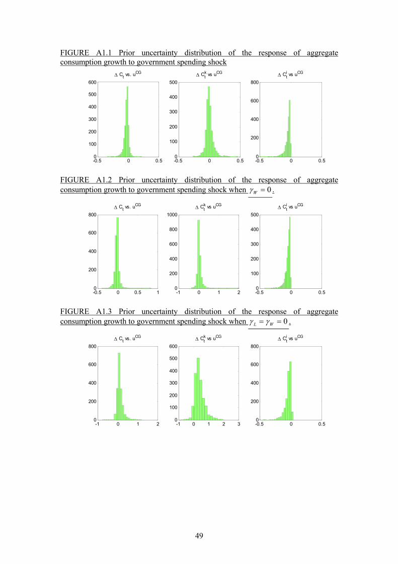
FIGURE A1.1 Prior uncertainty distribution of the response of aggregate consumption growth to government spending shock

Δ Ct vs. uCG Δ Ckt vs uCG Δ Ci

t vs uCG

600 500

-0.5 0 0.50

100

200

300

400

500

-0.5 0 0.50

100

200

300

400

800

-0.5 0 0.50

200

400

600

FIGURE A1.2 Prior uncertainty distribution of the response of aggregate consumption growth to government spending shock when 0=Wγ .

-0.5 0 0.5 10

200

400

600

800Δ Ct vs. uCG

-1 0 1 20

200

400

600

800

1000Δ Ck

t vs uCG

-0.5 0 0.50

100

200

300

400

500Δ Ci

t vs uCG

FIGURE A1.3 Prior uncertainty distribution of the response of aggregate consumption growth to government spending shock when 0== WL γγ .

-1 0 1 20

200

400

600

800Δ Ct vs. uCG

-1 0 1 2 30

100

200

300

400

500

600Δ Ck

t vs uCG

-0.5 0 0.50

200

400

600

800Δ Ci

t vs uCG

49

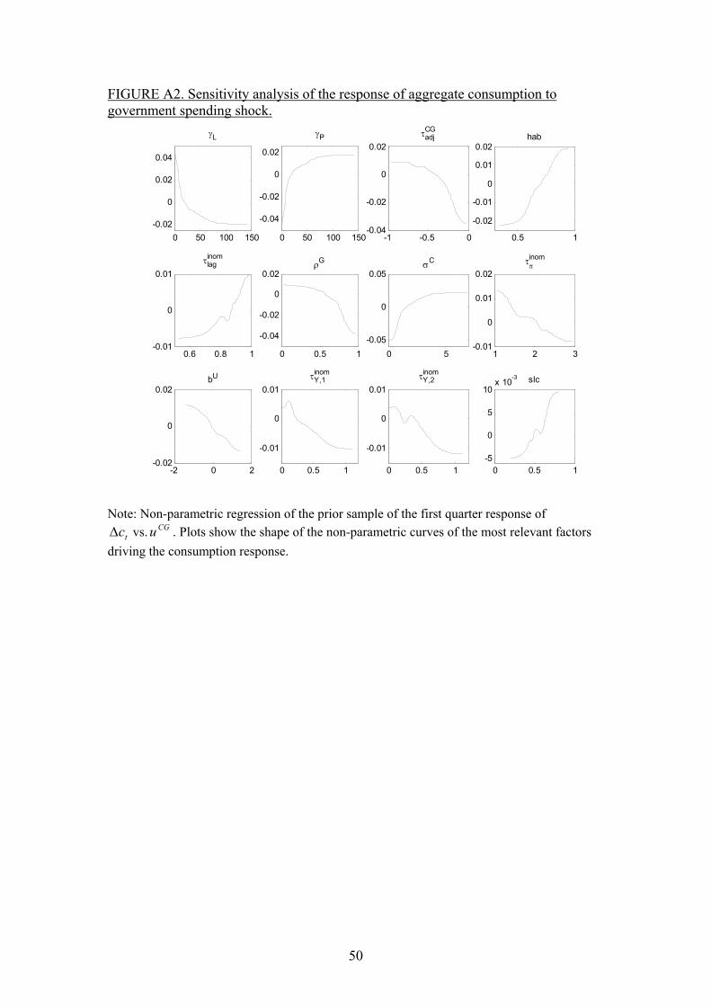
FIGURE A2. Sensitivity analysis of the response of aggregate consumption to government spending shock.

τCGadjγL γP hab

0.02 0.02

0 50 100 150-0.02

0

0.02

0.04

0 50 100 150

-0.04

-0.02

0

0.02

-1 -0.5 0-0.04

-0.02

0

0.5 1

-0.02

-0.01

0

0.01

τinomlag τinom

πρG σC

0.01 0.02 0.05 0.02

0.6 0.8 1-0.01

0

0 0.5 1

-0.04

-0.02

0

0 5-0.05

0

1 2 3-0.01

0

0.01

τinomY,1 τinom

Y,2bU

-2 0 2-0.02

0

0.02

0 0.5 1

-0.01

0

0.01

0 0.5 1

-0.01

0

0.01

0 0.5 1-5

0

5

10x 10

-3 slc

Note: Non-parametric regression of the prior sample of the first quarter response of

vs. . Plots show the shape of the non-parametric curves of the most relevant factors driving the consumption response.

tcΔ CGu

50

ANNEX 4 TABLE A1: Estimation Results for exogenous shocks

Prior posterior Parameter name distrib mean std mean std

kCσ gamma 0.05 0.03 0.0597 0.0107 τσ gamma 0.1 0.06 0.15 0.0246 PMσ gamma 0.02 0.015 0.0202 0.0038 PXσ gamma 0.1 0.06 0.0648 0.0355 EXσ gamma 0.005 0.03 0.0044 4.37E-04 CGσ gamma 0.05 0.03 0.0048 3.46E-04 IGσ gamma 0.05 0.03 0.0056 4.17E-04 Leisσ gamma 0.05 0.03 0.0283 0.0078 LOLσ gamma 0.005 0.003 0.0048 0.001 INOMσ gamma 0.003 0.0015 0.0013 9.88E-05

FBσ gamma 0.005 0.003 0.0017 2.40E-04 rpσ gamma 0.005 0.003 0.007 0.0017 TRσ gamma 0.05 0.03 0.0022 1.57E-04 Wσ gamma 0.05 0.03 0.0437 0.0156 UPσ gamma 0.05 0.03 0.0121 0.0013 Cρ beta 0.85 0.075 0.9144 0.0295 ηρ beta 0.5 0.2 0.1095 0.0771

Mηρ beta 0.85 0.075 0.9557 0.0164 Xηρ beta 0.85 0.075 0.8109 0.0668

CGρ beta 0.5 0.2 0.2983 0.1 IGρ beta 0.85 0.075 0.853 0.0797 Leisρ beta 0.85 0.075 0.975 0.0159 Lssρ beta 0.95 0.02 0.9334 0.0188 UIρ beta 0.5 0.2 0.6652 0.1409 PWPXρ beta 0.5 0.2 0.2159 0.0686

FBρ beta 0.85 0.075 0.9842 0.0103 rpρ beta 0.85 0.075 0.9148 0.0233 ucapρ beta 0.95 0.02 0.9517 0.0187 TRρ beta 0.85 0.075 0.8636 0.0428

51

Figure A3. Prior distributions (grey lines), posterior distributions (black lines) and posterior mode (dotted lines) of the estimated parameters.

52

53

54

55