64
Queueing Theory-1 Queueing Theory Queueing Theory Chapter 17
| Date post: | 30-Dec-2015 |
| Category: |
Documents |
| Upload: | elmo-perry |
| View: | 59 times |
| Download: | 0 times |

Queueing Theory-1
Queueing TheoryQueueing TheoryQueueing TheoryQueueing Theory
Chapter 17

Queueing Theory-2
Basic Queueing ProcessBasic Queueing ProcessBasic Queueing ProcessBasic Queueing Process
Arrivals • Arrival time
distribution• Calling population
(infinite or finite)
Queue• Capacity
(infinite or finite)• Queueing
discipline
Service• Number of servers
(one or more)• Service time
distribution
““Queueing System”Queueing System”
Queueing Theory-3
Examples and ApplicationsExamples and ApplicationsExamples and ApplicationsExamples and Applications
• Call centers (“help” desks, ordering goods)• Manufacturing• Banks• Telecommunication networks• Internet service• Intelligence gathering• Restaurants• Other examples….

Queueing Theory-4
Labeling Convention (Kendall-Lee)Labeling Convention (Kendall-Lee)Labeling Convention (Kendall-Lee)Labeling Convention (Kendall-Lee)
// // // // //Interarrival
timedistribution
Number of servers
Queueing discipline
System capacity
Calling population
size
Service time
distribution
M Markovian (exponential interarrival times, Poisson number of arrivals)
D Deterministic
Ek Erlang with shape parameter k
G General
FCFS first come, first served
LCFS last come, first served
SIRO service in random order
GD general discipline
Notes:

Queueing Theory-5
Labeling Convention (Kendall-Lee)Labeling Convention (Kendall-Lee)Labeling Convention (Kendall-Lee)Labeling Convention (Kendall-Lee)
Examples:
M/M/1
M/M/5
M/G/1
M/M/3/LCFS
Ek/G/2//10
M/M/1///100

Queueing Theory-6
Terminology and NotationTerminology and NotationTerminology and NotationTerminology and Notation
• State of the system Number of customers in the queueing system (includes customers in service)
• Queue length Number of customers waiting for service
= State of the system - number of customers being served
• N(t) = State of the system at time t, t ≥ 0
• Pn(t) = Probability that exactly n customers are in the queueing
system at time t

Queueing Theory-7
Terminology and NotationTerminology and NotationTerminology and NotationTerminology and Notation
n = Mean arrival rate (expected # arrivals per unit time) of new customers when n customers are in the system
• s = Number of servers (parallel service channels) n = Mean service rate for overall system
(expected # customers completing service per unit time) when n customers are in the system
Note: n represents the combined rate at which all busy servers (those serving customers) achieve service completion.

Queueing Theory-8
Terminology and NotationTerminology and NotationTerminology and NotationTerminology and Notation
When arrival and service rates are constant for all n,
= mean arrival rate (expected # arrivals per unit time)
= mean service rate for a busy server
1/ = expected interarrival time
1/ = expected service time
= /s = utilization factor for the service facility= expected fraction of time the system’s service capacity (s)
is being utilized by arriving customers ()
Queueing Theory-9
Terminology and NotationTerminology and NotationSteady StateSteady State
Terminology and NotationTerminology and NotationSteady StateSteady State
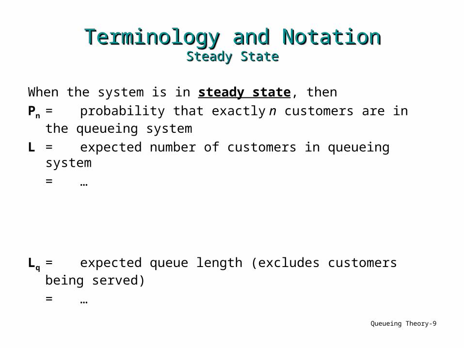
When the system is in steady state, then
Pn = probability that exactly n customers are in the queueing system
L = expected number of customers in queueing system
= …
Lq = expected queue length (excludes customers being served)
= …

Queueing Theory-10
Terminology and NotationTerminology and NotationSteady StateSteady State
Terminology and NotationTerminology and NotationSteady StateSteady State
When the system is in steady state, then
= waiting time in system (includes service time) for each individual customer
W = E[]
q = waiting time in queue (excludes service time) for each individual customer
Wq= E[q]
Queueing Theory-11
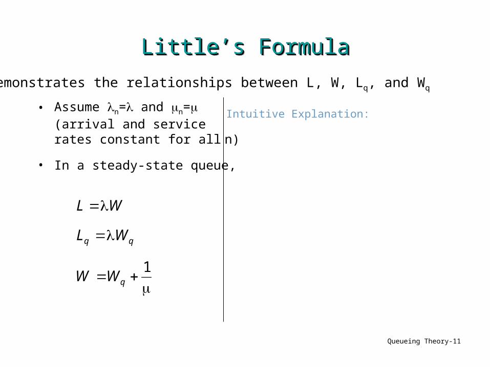
Little’s FormulaLittle’s FormulaLittle’s FormulaLittle’s Formula
• Assume n= and n= (arrival and service rates constant for all n)
• In a steady-state queue,
Intuitive Explanation:
1q
WW
WL
WL
Demonstrates the relationships between L, W, Lq, and Wq

Queueing Theory-12
Little’s Formula (continued)Little’s Formula (continued)Little’s Formula (continued)Little’s Formula (continued)
• This relationship also holds true for (expected arrival rate) when n are not equal.
Recall, Pn is the steady state probability of having n customers in the system
0
where
1
nnn
q
P
WW
WL
WL

Queueing Theory-13
Heading toward M/M/sHeading toward M/M/sHeading toward M/M/sHeading toward M/M/s
• The most widely studied queueing models are of the form M/M/s (s=1,2,…)
• What kind of arrival and service distributions does this model assume?
• Reviewing the exponential distribution….• If T ~ exponential(α), then
• A picture of the distribution:

Queueing Theory-14
Exponential Distribution ReviewedExponential Distribution ReviewedExponential Distribution ReviewedExponential Distribution Reviewed
If T ~ exponential(), then
000)(
ttetf
t
T
tt
u
uT eduetTPtF
1)()(0
E[T] = ______ Var(T) = ______
Queueing Theory-15
Property 1Property 1Strictly DecreasingStrictly DecreasingProperty 1Property 1
Strictly DecreasingStrictly Decreasing
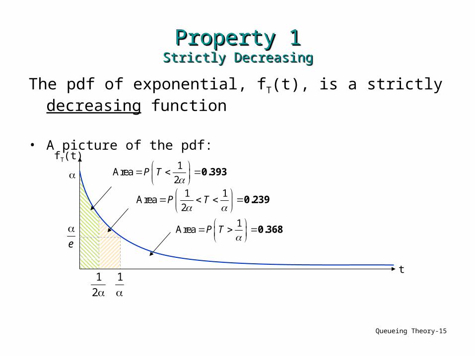
The pdf of exponential, fT(t), is a strictly decreasing function
• A picture of the pdf:
e
2
1
1
fT(t)
t
1Area
2P T
0.393
1 1Area
2P T
0.239
1Area P T
0.368

Queueing Theory-16
Property 2Property 2MemorylessMemoryless
Property 2Property 2MemorylessMemoryless
The exponential distribution has lack of memory
i.e. P(T > t+s | T > s) = P(T > t) for all s, t ≥ 0.
Example:
P(T > 15 min | T > 5 min) = P(T > 10 min)
The probability distribution has no memory of what has alreadyoccurred.

Queueing Theory-17
Property 2Property 2MemorylessMemoryless
Property 2Property 2MemorylessMemoryless
• Prove the memoryless property
• Is this assumption reasonable?– For interarrival times
– For service times

Queueing Theory-18
Property 3Property 3Minimum of ExponentialsMinimum of Exponentials
Property 3Property 3Minimum of ExponentialsMinimum of Exponentials
The minimum of several independent exponential random variables has an exponential distribution
If T1, T2, …, Tn are independent r.v.s, Ti ~ expon(i) and
U = min(T1, T2, …, Tn),
U ~expon( )
Example:If there are n servers, each with exponential service times with mean , then U = time until next service completion ~ expon(____)
1
n
ii

Queueing Theory-19
Property 4Property 4Poisson and ExponentialPoisson and Exponential
Property 4Property 4Poisson and ExponentialPoisson and Exponential
If the time between events, Xn ~ expon(), thenthe number of events occurring by time t, N(t) ~ Poisson(t)
Note:
E[X(t)] = αt, thus the expected number of events per unit time is α
( )
( ( ) ) for 0,1,2, ...!
n tt eP N t n n
n
( ( ) 0) tP N t e

Queueing Theory-20
Property 5Property 5ProportionalityProportionality
Property 5Property 5ProportionalityProportionality
For all positive values of t, and for small t,
P(T ≤ t+t | T > t) ≈ t
i.e. the probability of an event in interval t is proportional to the length of that interval

Queueing Theory-21
Property 6Property 6Aggregation and DisaggregationAggregation and Disaggregation
Property 6Property 6Aggregation and DisaggregationAggregation and Disaggregation
The process is unaffected by aggregation and disaggregation
Aggregation
N1 ~ Poisson(1)
N2 ~ Poisson(2)
Nk ~ Poisson(k)
= = 11++22+…++…+kk
N ~ Poisson(N ~ Poisson())
N1 ~ Poisson(p1)
N2 ~ Poisson(p2)
Nk ~ Poisson(pk)
N ~ Poisson(N ~ Poisson())
Disaggregation
p1
p2
pk… …
Note: p1+p2+…+pk=1

Queueing Theory-22
Back to QueueingBack to QueueingBack to QueueingBack to Queueing
• Remember that N(t), t ≥ 0, describes the state of the system:The number of customers in the queueing system at time t
• We wish to analyze the distribution of N(t) in steady state

Queueing Theory-23
Birth-and-Death ProcessesBirth-and-Death ProcessesBirth-and-Death ProcessesBirth-and-Death Processes
• If the queueing system is M/M/…/…/…/…, N(t) is a birth-and-death process
• A birth-and-death process either increases by 1 (birth), or decreases by 1 (death)
• General assumptions of birth-and-death processes:1. Given N(t) = n, the probability distribution of the time remaining until the
next birth is exponential with parameter λn
2. Given N(t) = n, the probability distribution of the time remaining until the next death is exponential with parameter μn
3. Only one birth or death can occur at a time

Queueing Theory-24
Rate DiagramsRate DiagramsRate DiagramsRate Diagrams
Queueing Theory-25
Steady-State Balance EquationsSteady-State Balance EquationsSteady-State Balance EquationsSteady-State Balance Equations

Queueing Theory-26
M/M/1 Queueing SystemM/M/1 Queueing SystemM/M/1 Queueing SystemM/M/1 Queueing System
• Simplest queueing system based on birth-and-death• We define
= mean arrival rate = mean service rate = / = utilization ratio
• We require < , that is < 1 in order to have a steady state– Why?
Rate DiagramRate Diagram
0 1 2 3 4 …

Queueing Theory-27
M/M/1 Queueing System M/M/1 Queueing System Steady-State ProbabilitiesSteady-State Probabilities
M/M/1 Queueing System M/M/1 Queueing System Steady-State ProbabilitiesSteady-State Probabilities
Calculate Pn, n = 0, 1, 2, …
Queueing Theory-28
M/M/1 Queueing System M/M/1 Queueing System L, LL, Lqq, W, W, W, Wqq
M/M/1 Queueing System M/M/1 Queueing System L, LL, Lqq, W, W, W, Wqq
Calculate L, Lq, W, Wq

Queueing Theory-29
M/M/1 Example: ERM/M/1 Example: ERM/M/1 Example: ERM/M/1 Example: ER
• Emergency cases arrive independently at random• Assume arrivals follow a Poisson input process (exponential
interarrival times) and that the time spent with the ER doctor is exponentially distributed
• Average arrival rate = 1 patient every ½ hour
=
• Average service time = 20 minutes to treat each patient
=
• Utilization
=
Queueing Theory-30
M/M/1 Example: ERM/M/1 Example: ERQuestionsQuestions
M/M/1 Example: ERM/M/1 Example: ERQuestionsQuestions
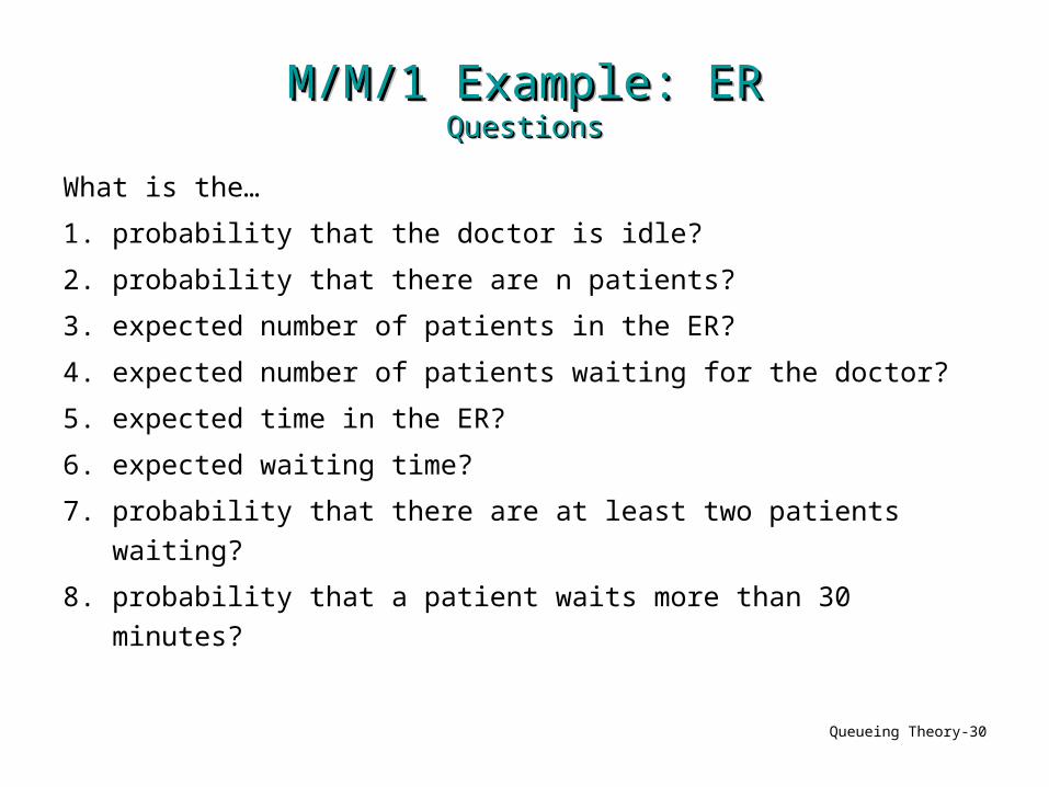
What is the…
1. probability that the doctor is idle?
2. probability that there are n patients?
3. expected number of patients in the ER?
4. expected number of patients waiting for the doctor?
5. expected time in the ER?
6. expected waiting time?
7. probability that there are at least two patients waiting?
8. probability that a patient waits more than 30 minutes?
Queueing Theory-31
Car Wash ExampleCar Wash ExampleCar Wash ExampleCar Wash Example
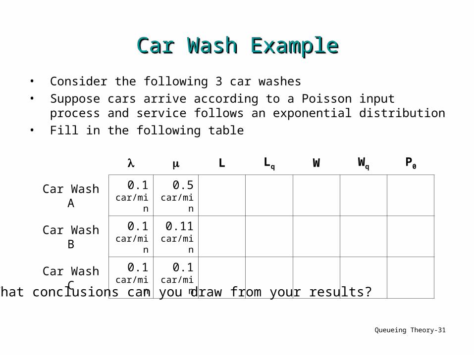
• Consider the following 3 car washes• Suppose cars arrive according to a Poisson input process and
service follows an exponential distribution• Fill in the following table
What conclusions can you draw from your results?
L Lq W Wq P0
Car Wash A 0.1 car/min
0.5 car/min
Car Wash B 0.1 car/min
0.11 car/min
Car Wash C 0.1 car/min
0.1 car/min

Queueing Theory-32
M/M/s Queueing SystemM/M/s Queueing SystemM/M/s Queueing SystemM/M/s Queueing System
• We define = mean arrival rate = mean service rate s = number of servers (s > 1) = / s = utilization ratio
• We require < s , that is < 1 in order to have a steady state
Rate DiagramRate Diagram
0 1 2 3 4 …
Queueing Theory-33
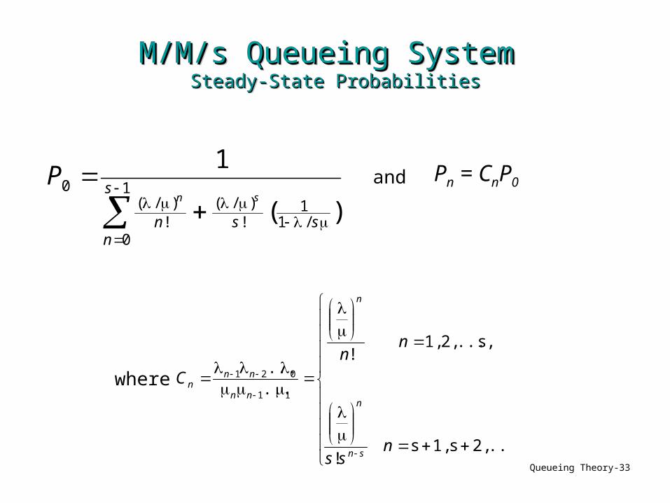
M/M/s Queueing System M/M/s Queueing System Steady-State ProbabilitiesSteady-State Probabilities
M/M/s Queueing System M/M/s Queueing System Steady-State ProbabilitiesSteady-State Probabilities
... 2,s 1,s!
s ..., 2, 1,!
......
11
021
nss
nn
C
sn
n
n
nn
nnn
)(
1
/11
!)/(
1
0!)/(
0
ss
s
nn
sn
P and Pn = CnP0
where
Queueing Theory-34
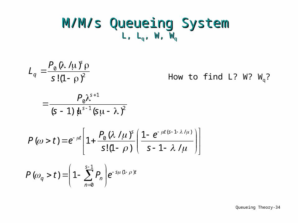
M/M/s Queueing System M/M/s Queueing System L, LL, Lqq, W, W, W, Wqq
M/M/s Queueing System M/M/s Queueing System L, LL, Lqq, W, W, W, Wqq
21
10
20
)()!1(
)1(!
)/(
ss
P
s
PL
s
s
s
q
/1
1
)1(!
)/(1)(
)/1(0
s
e
s
PetP
stst
How to find L? W? Wq?
tss
nnq ePtP )1(
1
0
1)(
Queueing Theory-35
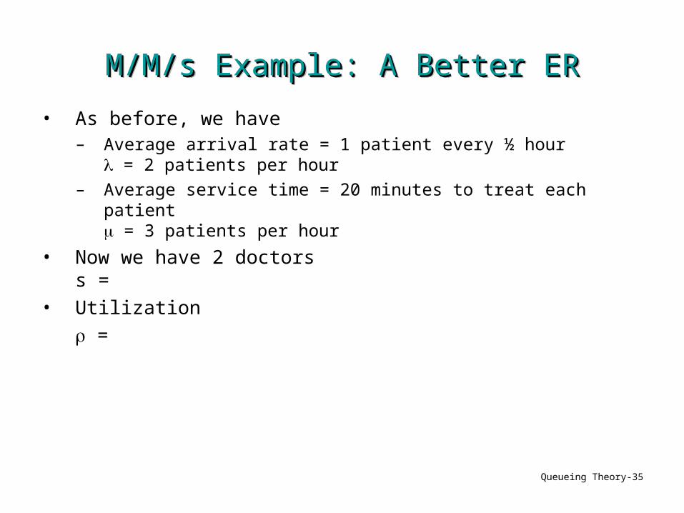
M/M/s Example: A Better ERM/M/s Example: A Better ERM/M/s Example: A Better ERM/M/s Example: A Better ER
• As before, we have– Average arrival rate = 1 patient every ½ hour
= 2 patients per hour
– Average service time = 20 minutes to treat each patient = 3 patients per hour
• Now we have 2 doctorss =
• Utilization
=

Queueing Theory-36
M/M/s Example: ERM/M/s Example: ERQuestionsQuestions
M/M/s Example: ERM/M/s Example: ERQuestionsQuestions
What is the…
1. probability that both doctors are idle?
a) probability that exactly one doctor is idle?
2. probability that there are n patients?
3. expected number of patients in the ER?
4. expected number of patients waiting for a doctor?
5. expected time in the ER?
6. expected waiting time?
7. probability that there are at least two patients waiting?
8. probability that a patient waits more than 30 minutes?

Queueing Theory-37
Performance Measurements
s = 1 s = 2
ρ 2/3 1/3
L 2 3/4
Lq 4/3 1/12
W 1 hr 3/8 hr
Wq 2/3 hr 1/24 hr
P(at least two patients waiting in queue)
0.296 0.0185
P(a patient waits more than 30 minutes)
0.404 0.022

Queueing Theory-38
Travel Agency ExampleTravel Agency ExampleTravel Agency ExampleTravel Agency Example
• Suppose customers arrive at a travel agency according to a Poisson input process and service times have an exponential distribution
• We are given = .10/minute = 1 customer every 10 minutes = .08/minute = 8 customers every 100 minutes
• If there were only one server, what would happen?• How many servers would you recommend?

Queueing Theory-39
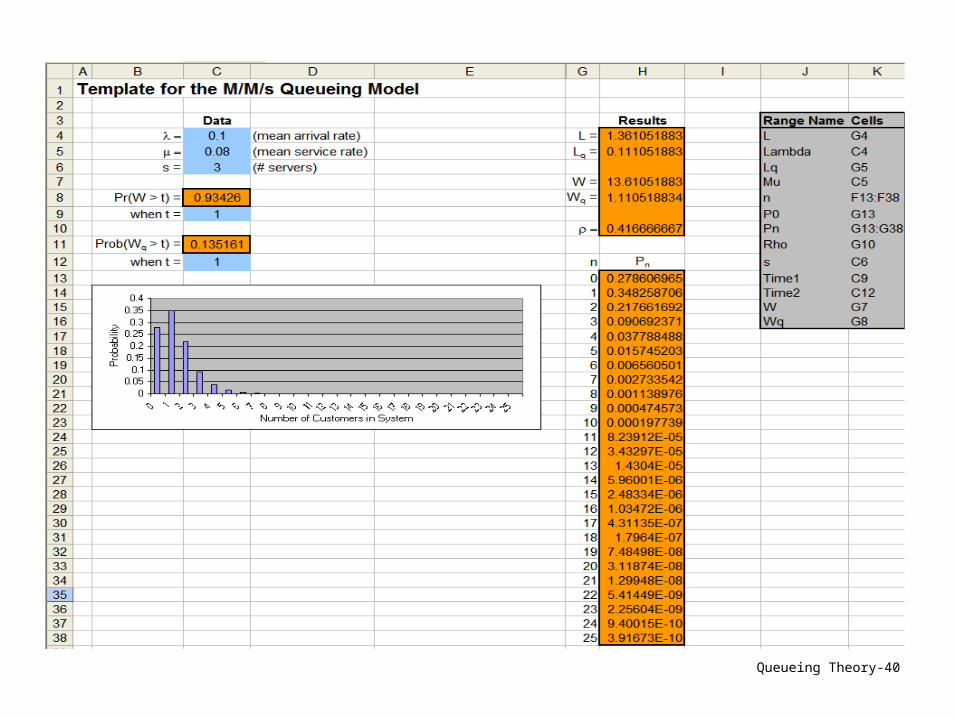
Queueing Theory-40

Queueing Theory-41

Queueing Theory-42
Single Queue vs. Multiple QueuesSingle Queue vs. Multiple QueuesSingle Queue vs. Multiple QueuesSingle Queue vs. Multiple Queues
• Would you ever want to keep separate queues for separate servers?
Single queue
Multiple queues
vs.

Queueing Theory-43
Bank ExampleBank ExampleBank ExampleBank Example
• Suppose we have two tellers at a bank• Compare the single server and multiple server models• Assume = 2, = 3
L Lq W Wq P0

Queueing Theory-44
Bank ExampleBank ExampleContinuedContinued
Bank ExampleBank ExampleContinuedContinued
• Suppose we now have 3 tellers• Again, compare the two models
Queueing Theory-45
M/M/s//K Queueing ModelM/M/s//K Queueing Model(Finite Queue Variation of M/M/s)(Finite Queue Variation of M/M/s)
M/M/s//K Queueing ModelM/M/s//K Queueing Model(Finite Queue Variation of M/M/s)(Finite Queue Variation of M/M/s)
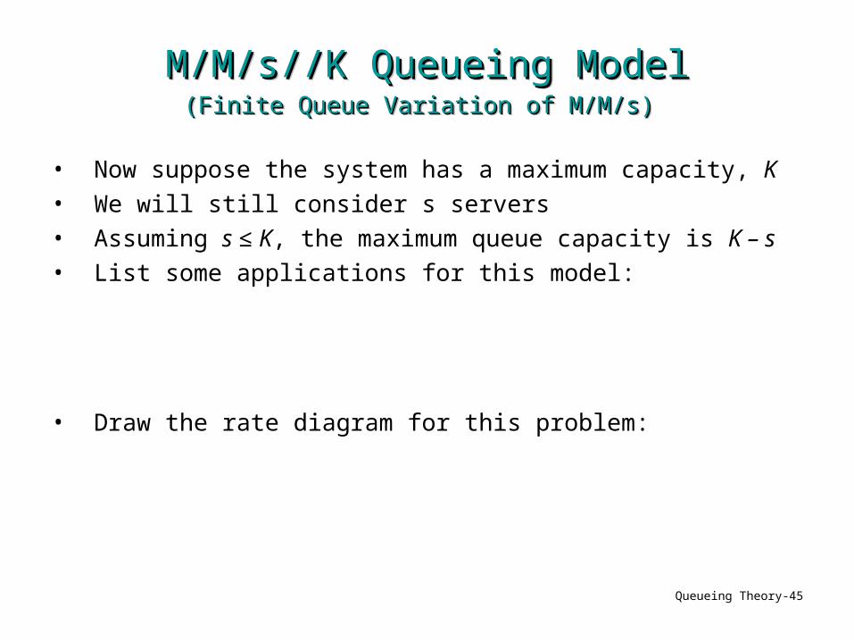
• Now suppose the system has a maximum capacity, K• We will still consider s servers• Assuming s ≤ K, the maximum queue capacity is K – s• List some applications for this model:
• Draw the rate diagram for this problem:

Queueing Theory-46
M/M/s//K Queueing ModelM/M/s//K Queueing Model(Finite Queue Variation of M/M/s)(Finite Queue Variation of M/M/s)
M/M/s//K Queueing ModelM/M/s//K Queueing Model(Finite Queue Variation of M/M/s)(Finite Queue Variation of M/M/s)
Balance equations: Rate In = Rate Out
Rate DiagramRate Diagram
0 1 2 3 4 …
Queueing Theory-47
M/M/s//K Queueing ModelM/M/s//K Queueing Model(Finite Queue Variation of M/M/s)(Finite Queue Variation of M/M/s)
M/M/s//K Queueing ModelM/M/s//K Queueing Model(Finite Queue Variation of M/M/s)(Finite Queue Variation of M/M/s)
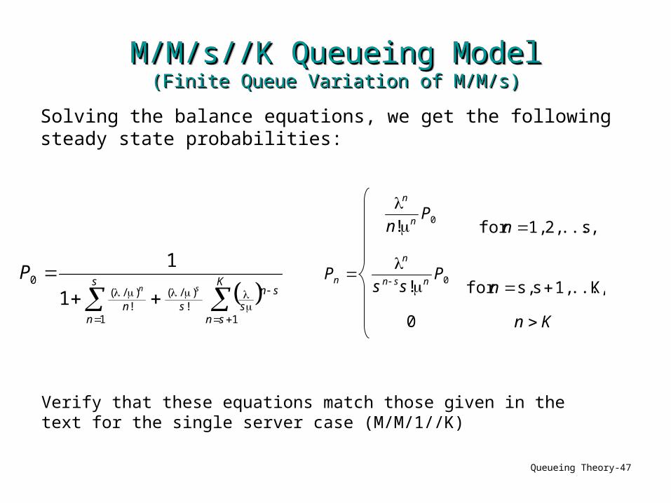
Solving the balance equations, we get the following steady state probabilities:
Kn
nP
ss
nP
n
Pnsn
n
n
n
n
0
K ..., 1,s s, for!
s ..., 2, 1, for!
0
0
Verify that these equations match those given in the text for the single server case (M/M/1//K)
K
sn
sn
ss
s
nn
sn
P
1!
)/(
1!)/(
0
1
1

Queueing Theory-48
M/M/s//K Queueing ModelM/M/s//K Queueing Model(Finite Queue Variation of M/M/s)(Finite Queue Variation of M/M/s)
M/M/s//K Queueing ModelM/M/s//K Queueing Model(Finite Queue Variation of M/M/s)(Finite Queue Variation of M/M/s)
1
0
1
0
20
1
/ where)],1()(1[)1(!
)/(
s
nnq
s
nn
sKsKs
q
PsLnPL
ssKs
PL
WL qq WL )1(0
Kn
nn PP
To find W and Wq:
Although L ≠ W and Lq ≠ Wq because n is not equal for all n,
and where

Queueing Theory-49
M/M/s///N Queueing ModelM/M/s///N Queueing Model(Finite Calling Population Variation of M/M/s)(Finite Calling Population Variation of M/M/s) M/M/s///N Queueing ModelM/M/s///N Queueing Model
(Finite Calling Population Variation of M/M/s)(Finite Calling Population Variation of M/M/s)
• Now suppose the calling population is finite• We will still consider s servers• Assuming s ≤ K, the maximum queue capacity is K – s• List some applications for this model:
• Draw the rate diagram for this problem:

Queueing Theory-50
M/M/s///N Queueing ModelM/M/s///N Queueing Model(Finite Calling Population Variation of M/M/s)(Finite Calling Population Variation of M/M/s)M/M/s///N Queueing ModelM/M/s///N Queueing Model
(Finite Calling Population Variation of M/M/s)(Finite Calling Population Variation of M/M/s)
Balance equations: Rate In = Rate Out
Rate DiagramRate Diagram
0 1 2 3 4 …

Queueing Theory-51
M/M/s///N ResultsM/M/s///N ResultsM/M/s///N ResultsM/M/s///N Results
1
0
0
!)!(!
!)!(!
1s
n
N
sn
n
sn
n
ssnNN
nnNN
P
Nn for0
Nn for!)!(
!
,...,1,0 for!)!(
!
0
0
sPssnN
N
snPnnN
N
Pn
sn
n
n
N
snnq PsnL )(
1
0
1
0
1s
nnq
s
nn PsLnPL
Queueing Theory-52
Queueing Models with Nonexponential DistributionsQueueing Models with Nonexponential DistributionsQueueing Models with Nonexponential DistributionsQueueing Models with Nonexponential Distributions
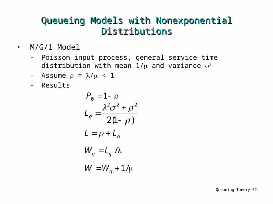
• M/G/1 Model– Poisson input process, general service time distribution with mean 1/
and variance 2
– Assume = / < 1
– Results
10P
/1
/
q
WW
LW
q
q
LL
L
)1(2
222

Queueing Theory-53
Queueing Models with Nonexponential DistributionsQueueing Models with Nonexponential DistributionsQueueing Models with Nonexponential DistributionsQueueing Models with Nonexponential Distributions
• M/Ek/1 Model
– Erlang: Sum of exponentials
– Think it would be useful?
– Can readily apply the formulae on previous slide where
• Other models– M/D/1
– Ek/M/1
– etc
22 1
k
0t for
!1)( 1
tkkk
T etk
ktf

Queueing Theory-54
Application of Queueing TheoryApplication of Queueing TheoryApplication of Queueing TheoryApplication of Queueing Theory
• We can use the results for the queueing models when making decisions on design and/or operations
• Some decisions that we can address– Number of servers
– Efficiency of the servers
– Number of queues
– Amount of waiting space in the queue
– Queueing disciplines
Queueing Theory-55
Number of ServersNumber of ServersNumber of ServersNumber of Servers
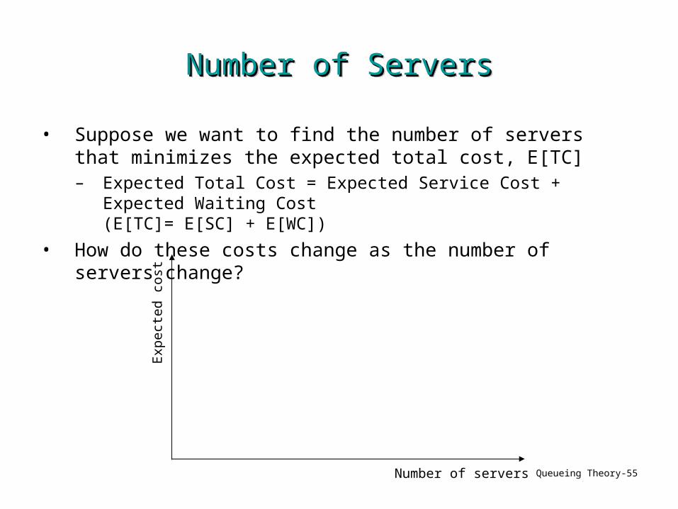
• Suppose we want to find the number of servers that minimizes the expected total cost, E[TC]– Expected Total Cost = Expected Service Cost + Expected Waiting Cost
(E[TC]= E[SC] + E[WC])
• How do these costs change as the number of servers change?
Number of servers
Exp
ecte
d co
st
Queueing Theory-56
Repair Person ExampleRepair Person ExampleRepair Person ExampleRepair Person Example
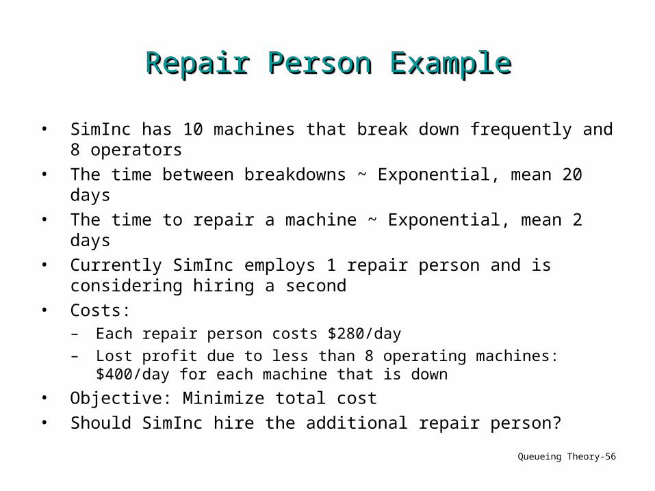
• SimInc has 10 machines that break down frequently and 8 operators
• The time between breakdowns ~ Exponential, mean 20 days• The time to repair a machine ~ Exponential, mean 2 days• Currently SimInc employs 1 repair person and is considering hiring
a second• Costs:
– Each repair person costs $280/day
– Lost profit due to less than 8 operating machines:$400/day for each machine that is down
• Objective: Minimize total cost• Should SimInc hire the additional repair person?

Queueing Theory-57
Repair Person ExampleRepair Person ExampleProblem ParametersProblem Parameters
Repair Person ExampleRepair Person ExampleProblem ParametersProblem Parameters
• What type of problem is this?– M/M/1
– M/M/s
– M/M/s/K
– M/G/1
– M/M/s finite calling population
– M/Ek/1
– M/D/1
• What are the values of and ?
Queueing Theory-58
Repair Person ExampleRepair Person ExampleRate DiagramsRate Diagrams
Repair Person ExampleRepair Person ExampleRate DiagramsRate Diagrams
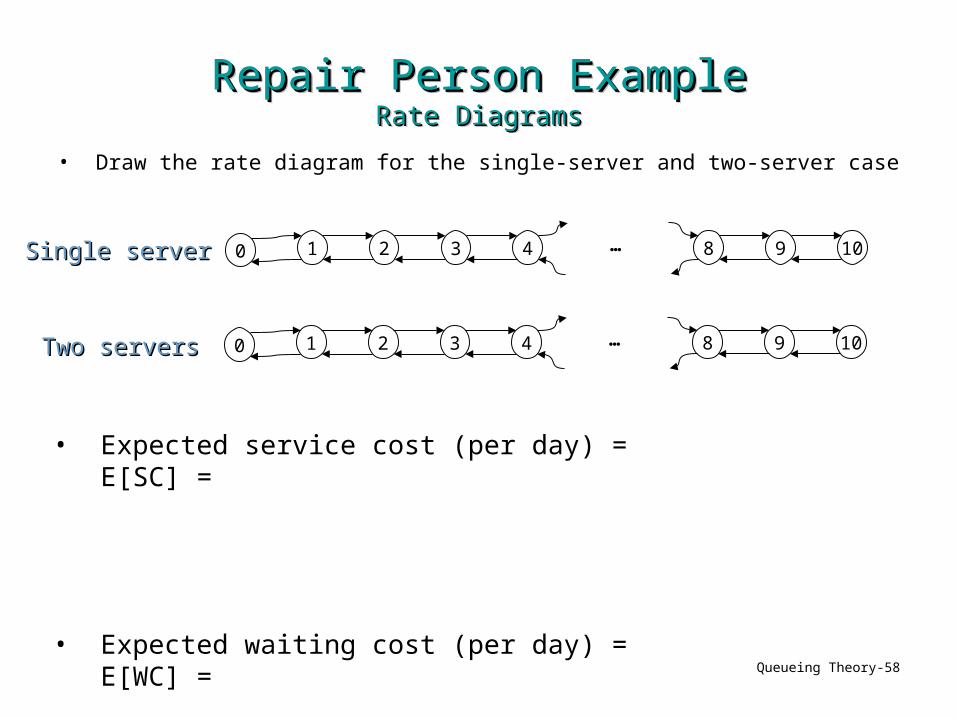
• Draw the rate diagram for the single-server and two-server case
Single serverSingle server 0 1 2 3 4 …
• Expected service cost (per day) = E[SC] =
• Expected waiting cost (per day) = E[WC] =
1098
Two serversTwo servers 0 1 2 3 4 … 1098

Queueing Theory-59
Repair Person ExampleRepair Person ExampleSteady-State ProbabilitiesSteady-State Probabilities
Repair Person ExampleRepair Person ExampleSteady-State ProbabilitiesSteady-State Probabilities
• Write the balance equations for each case
• How to find E[WC] for s=1? s=2?

Queueing Theory-60
Repair Person ExampleRepair Person ExampleE[WC] CalculationsE[WC] Calculations
Repair Person ExampleRepair Person ExampleE[WC] CalculationsE[WC] Calculations
N=n g(n)s=1 s=2
Pn g(n) Pn Pn g(n) Pn
0 0 0.271 0 0.433 0
1 0 0.217 0 0.346 0
2 0 0.173 0 0.139 0
3 400 0.139 56 0.055 24
4 800 0.097 78 0.019 16
5 1200 0.058 70 0.006 8
6 1600 0.029 46 0.001 0
7 2000 0.012 24 0.0003 0
8 2400 0.003 7 0.00004 0
9 2800 0.0007 0 0.000004 0
10 3200 0.00007 0 0.0000002 0
E[WC] $281/day $48/day

Queueing Theory-61
Repair Person ExampleRepair Person ExampleResultsResults
Repair Person ExampleRepair Person ExampleResultsResults
• We get the following results
s E[SC]: E[WC]: E[TC]:
1 $280/day $281/day $561/day
2 $560/day $48/day $608/day
≥ 3 ≥ $840/day ≥ $0/day ≥ $840/day
• What should SimInc do?

Queueing Theory-62
Supercomputer ExampleSupercomputer ExampleSupercomputer ExampleSupercomputer Example
• Emerald University has plans to lease a supercomputer• They have two options
• Students and faculty jobs are submitted on average of 20 jobs/day, distributed Poisson
i.e. Time between submissions ~ __________
• Which computer should Emerald University lease?
SupercomputerMean number of jobs
per dayCost per day
MBI 30 jobs/day $5,000/day
CRAB 25 jobs/day $3,750/day

Queueing Theory-63
Supercomputer ExampleSupercomputer ExampleWaiting Cost FunctionWaiting Cost Function
Supercomputer ExampleSupercomputer ExampleWaiting Cost FunctionWaiting Cost Function
• Assume the waiting cost is not linear:
h() = 500 + 400 2 ( = waiting time in days)
• What distribution do the waiting times follow?
• What is the expected waiting cost, E[WC]?

Queueing Theory-64
Supercomputer ExampleSupercomputer ExampleResultsResults
Supercomputer ExampleSupercomputer ExampleResultsResults
• Next incorporate the leasing cost to determine the expected total cost, E[TC]
• Which computer should the university lease?


