65
Queueing Theory
| Date post: | 22-Dec-2015 |
| Category: |
Documents |
| Upload: | samantha-powell |
| View: | 219 times |
| Download: | 5 times |

Queueing Theory

Operations -- Prof. Juran 2
Overview• Basic definitions and metrics• Examples of some theoretical models

Operations -- Prof. Juran 3
Basic Queueing TheoryA set of mathematical tools for the analysis of probabilistic systems of customers and servers.
Can be traced to the work of A. K. Erlang, a Danish mathematician who studied telephone traffic congestion in the first decade of the 20th century.
Applications:Service OperationsManufacturingSystems Analysis

Operations -- Prof. Juran 4
Agner Krarup Erlang
(1878 - 1929)

Components of a Queuing System
Arrival Process
ServersQueue or Waiting Line
Service Process
Exit

Customer Population Sources
Population Source
Finite Infinite
Example: Number of machines needing repair when a company only has three machines.
Example: Number of machines needing repair when a company only has three machines.
Example: The number of people who could wait in a line for gasoline.
Example: The number of people who could wait in a line for gasoline.

Service Pattern
Service Pattern
Constant Variable
Example: Items coming down an automated assembly line.
Example: Items coming down an automated assembly line.
Example: People spending time shopping.
Example: People spending time shopping.

Examples of Queue Structures
Single Channel
Multichannel
SinglePhase Multiphase
One-personbarber shop
Car wash
Hospitaladmissions
Bank tellers’windows

Balking and Reneging
No Way! No Way!
Reneging: Joining the queue, then leaving
Balking: Arriving, but not joining the queue
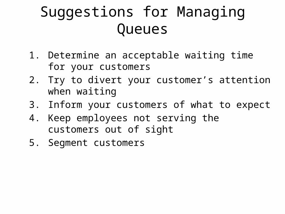
Suggestions for Managing Queues
1. Determine an acceptable waiting time for your customers
2. Try to divert your customer’s attention when waiting
3. Inform your customers of what to expect4. Keep employees not serving the customers out
of sight5. Segment customers

Suggestions for Managing Queues
6. Train your servers to be friendly
7. Encourage customers to come during the slack periods
8. Take a long-term perspective toward getting rid of the queues

Operations -- Prof. Juran 12
Arrival Rate refers to the average number of customers who require service within a specific period of time.
A Capacitated Queue is limited as to the number of customers who are allowed to wait in line.
Customers can be people, work-in-process inventory, raw materials, incoming digital messages, or any other entities that can be modeled as lining up to wait for some process to take place.
A Queue is a set of customers waiting for service.

Operations -- Prof. Juran 13
Queue Discipline refers to the priority system by which the next customer to receive service is selected from a set of waiting customers. One common queue discipline is first-in-first-out, or FIFO.
A Server can be a human worker, a machine, or any other entity that can be modeled as executing some process for waiting customers.
Service Rate (or Service Capacity) refers to the overall average number of customers a system can handle in a given time period.
Stochastic Processes are systems of events in which the times between events are random variables. In queueing models, the patterns of customer arrivals and service are modeled as stochastic processes based on probability distributions.
Utilization refers to the proportion of time that a server (or system of servers) is busy handling customers.

Operations -- Prof. Juran 14
In the literature, queueing models are described by a series of symbols and slashes, such as A/B/X/Y/Z, where
• A indicates the arrival pattern, • B indicates the service pattern, • X indicates the number of parallel servers, • Y indicates the queue’s capacity, and • Z indicates the queue discipline.
We will be concerned primarily with the M/M/1 queue, in which the letter M indicates that times between arrivals and times between services both can be modeled as being exponentially distributed. The number 1 indicates that there is one server.
We will also study some M/M/s queues, where s is some number greater than 1.
Operations -- Prof. Juran 15
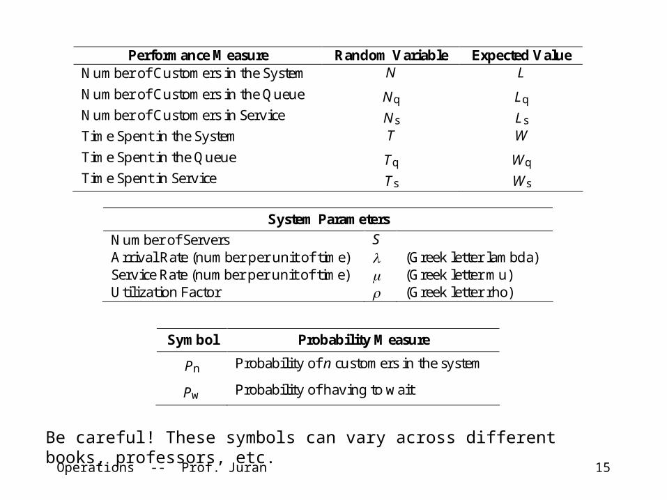
Be careful! These symbols can vary across different books, professors, etc.
Performance Measure Random Variable Expected Value Number of Customers in the System N L
Number of Customers in the Queue Nq Lq Number of Customers in Service Ns Ls Time Spent in the System T W
Time Spent in the Queue Tq Wq Time Spent in Service Ts Ws
System Parameters Number of Servers S Arrival Rate (number per unit of time) (Greek letter lambda) Service Rate (number per unit of time) (Greek letter mu) Utilization Factor (Greek letter rho)
Symbol Probability Measure
Pn Probability of n customers in the system
Pw Probability of having to wait

Operations -- Prof. Juran 16
General(all queue models)
Single Server M/M/S
M/M/2(Model 3)
M/D/1(Model 2)
M/M/1(Model 1)
Single PhaseInfinite SourceFCFS Discipline
Infinite Queue Length

Operations -- Prof. Juran 17
John D. C. Little
1928 —
General Formulas

Operations -- Prof. Juran 18
The single most important formula in queueing theory is called Little’s Law:
Little’s Law applies to any subsystem as well. For example,
Average time in system L
W i
Average customers in system WL ii
Arrival Rate WL
iii
Average time in queue
LW iv

Operations -- Prof. Juran 19
L as a Function of Rho
0
20
40
60
80
100
120
140
160
180
200
0 0.1 0.2 0.3 0.4 0.5 0.6 0.7 0.8 0.9 1
Rho
L

Operations -- Prof. Juran 20
General Single-Server Formulas
Average time in system 1
qWW v
Average time in queue
LW vi
Operations -- Prof. Juran 21
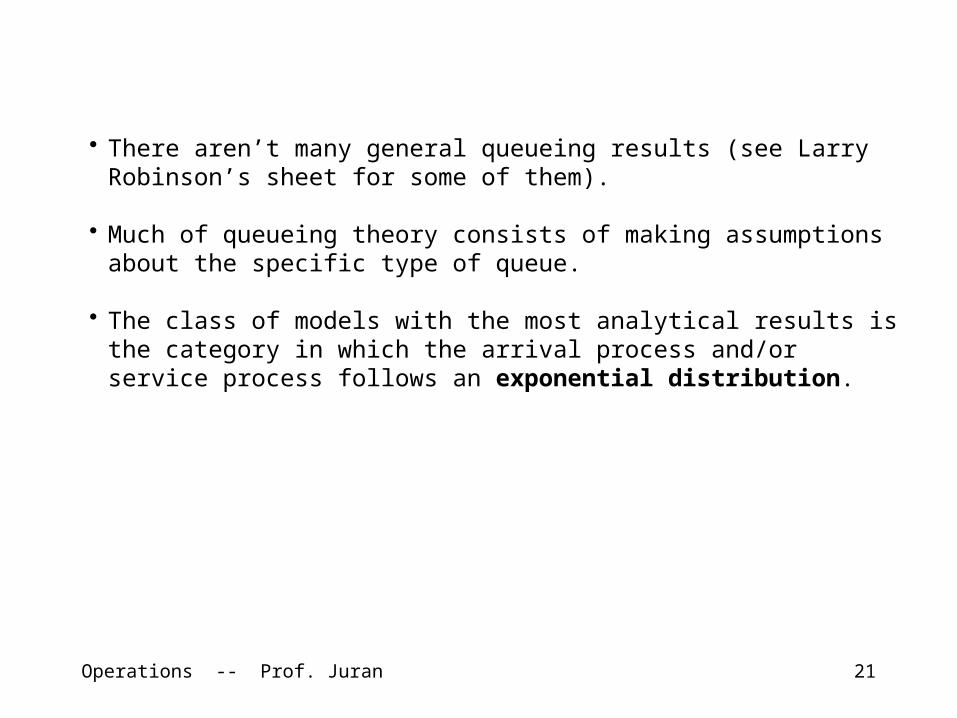
• There aren’t many general queueing results (see Larry Robinson’s sheet for some of them).
• Much of queueing theory consists of making assumptions about the specific type of queue.
• The class of models with the most analytical results is the category in which the arrival process and/or service process follows an exponential distribution.

Operations -- Prof. Juran 22
Example: General Formula
I Average line lengthc Number of serversCi Coefficient of variation; arrival processCp Coefficient of variation; service process
Coefficient of Variation:
𝐼 ≅ 𝜌√2 (𝑐+1 )
1−𝜌×𝐶𝑖
❑❑2 +𝐶𝑝
❑❑2
2

Operations -- Prof. Juran 23
Andrey Markov
(Андрей Андреевич Марков) 1856 — 1922

Operations -- Prof. Juran 24
Time between Events
Pro
bab
ilit
y
tetTP
The Exponential Distribution
T is a continuous positive random number.
t is a specific value of T.

Operations -- Prof. Juran 25
Example:
If the average time between arrivals is 45 seconds and inter-arrival times are exponentially distributed, what is the probability that two sequential arrivals will be more than 60 seconds apart?
Remember lambda is in “events per time unit”, so
02222.0451
60TP te
60*02222.0718.2
2636.0

Operations -- Prof. Juran 26
2636.060 TP

Operations -- Prof. Juran 27
Here’s how to do this calculation in Excel:
The EXP function raises e to the power of whatever number is in parentheses.
1234
D E F G
lambda 0.02222t 60
0.2636=EXP(-E2*E3)
=1/45

Operations -- Prof. Juran 28
Remember that the exponential distribution has a really long tail. In probability-speak, it has strong right-skewness, and there are outliers with very large values.
In fact, the probability of any one inter-event time being longer than the mean inter-event time is:
In other words, only 37% of inter-event times will be longer than the expected value of the inter-event times.
This counter-intuitive result is because some of the 37% are really, really long.
1
TP 3679.0

Operations -- Prof. Juran 29
1
TP 3679.0

Operations -- Prof. Juran 30
Other Facts about the Exponential Distribution
• “Memoryless” property: The expected time until the next event is independent of how long it’s been since the previous event
• The mean is equal to the standard deviation (so the CV is always 1)
• Analogous to the discrete Geometric distribution

Operations -- Prof. Juran 31
Siméon Denis Poisson
1781 — 1840

Operations -- Prof. Juran 32
If the random time between events is exponentially distributed, then the random number of events in any given period of time follows a Poisson process.
A Poisson random variable is discrete. The number of events n (i.e. arrivals) in a certain space of time must be an integer.
n is a positive random integer (sometimes zero).

Operations -- Prof. Juran 33
In English: The probability of exactly n events within t time units.
!n
etnP
tn
t

Operations -- Prof. Juran 34
Poisson distribution; λ = 7.5
0.00
0.02
0.04
0.06
0.08
0.10
0.12
0.14
0.16
0 1 2 3 4 5 6 7 8 9 10 11 12 13 14 15 16 17 18 19 20 21 22 23 24 25
Number of Events in 1 Time Unit
Pro
babi
lity
!n
etnP
tn
t

Operations -- Prof. Juran 35
222324252627282930313233343536373839
E F G H Ilambda 7.5
0 0.00055311 0.00414812 0.01555553 0.03888874 0.07291645 0.10937466 0.13671827 0.14648388 0.13732869 0.114440510 0.085830411 0.058520712 0.036575413 0.021101214 0.011304215 0.0056521
=POISSON(E25,$F$22,0)
0.00
0.02
0.04
0.06
0.08
0.10
0.12
0.14
0.16
0 1 2 3 4 5 6 7 8 9 10 11 12 13 14 15 16 17 18 19 20 21 22 23 24 25
Number of Events
Prob
abil
ity
222324252627282930313233343536373839
E F G H Ilambda 7.5
0 0.00055311 0.00470122 0.02025673 0.05914554 0.13206195 0.24143656 0.37815477 0.52463858 0.66196719 0.776407610 0.862238011 0.920758712 0.957334113 0.978435314 0.989739615 0.9953917
=POISSON(E25,$F$22,1)
0.0
0.1
0.2
0.3
0.4
0.5
0.6
0.7
0.8
0.9
1.0
0 1 2 3 4 5 6 7 8 9 10 11 12 13 14 15 16 17 18 19 20 21 22 23 24 25
Number of Events
Prob
abil
ity

Operations -- Prof. Juran 36
The Excel formula is good for figuring out the probability distribution for the number of events in one time unit. Here is a more general approach:
This gives the probability of exactly fifteen events in three time units, when the average number of events per time unit is 7.5.
You could adapt the Excel formula for general purposes by re-defining what “one time unit” means.
131415161718
H I J K L M Nn 15lambda 7.5e 2.718t 3
0.02481
=EXP(1)
=(((I14*I16)^I13)*((I15)^(-I14*I16)))/(FACT(I13))

Waiting Line Models
These four models share the following characteristics:• Single Phase• Poisson Arrivals• FCFS Discipline• Unlimited Queue Capacity
Model Layout Source Population Service Pattern 1 Single Channel Infinite Exponential 2 Single Channel Infinite Deterministic 3 Multichannel Infinite Exponential 4 Single or Multi Finite Exponential

Operations -- Prof. Juran 38
Model 1 (M/M/1) Formulas
Utilization vii
Average customers in the system
1
L viii
L ix
Operations -- Prof. Juran 39
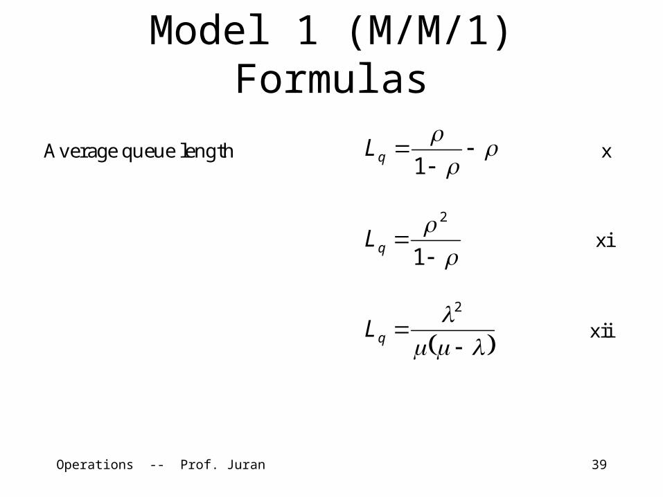
Model 1 (M/M/1) Formulas
Average queue length
1qL x
1
2
qL xi
2
qL xii

Operations -- Prof. Juran 40
Model 1 (M/M/1) Formulas
Average time in system
1
W xiii
Average time in queue
qW xiv
L
Wq xv

Operations -- Prof. Juran 41
Model 1 (M/M/1) Formulas
Probability of a specific number of customers in the system
n
nP
1 xvi
nnNP xvii
Probability of no wait
10P xviii

Example: Model 1 (M/M/1)
Assume a drive-up window at a fast food restaurant.Customers arrive at the rate of 25 per hour.The employee can serve one customer every two minutes.Assume Poisson arrival and exponential service rates.
Determine:A. What is the average utilization of the employee?B. What is the average number of customers in line?C. What is the average number of customers in the
system?D. What is the average waiting time in line?E. What is the average waiting time in the system?F. What is the probability that exactly two cars will be
in the system?

.8333 = cust/hr 30cust/hr 25
= =
cust/hr 30 = mins) (1hr/60 mins 2
customer 1 =
cust/hr 25 =
Example: Model 1 (M/M/1)
A) What is the average utilization of the employee?

Example: Model 1
B) What is the average number of customers in line?
4.167 = 25)-30(30
(25) =
) - ( =
22
qL
C) What is the average number of customers in the system?
5 = 25)-(30
25 =
- =
L

Example: Model 1
D) What is the average waiting time in line?
mins 10 = hrs.1667 =
=qL
qW
E) What is the average time in the system?
mins 12 = hrs .2 = =L
W

Example: Model 1F) What is the probability that exactly two cars
will be in the system (one being served and the other waiting in line)?
n
n μλ
μλ
-p
1
1157.03025
3025
12
2
-p

Operations -- Prof. Juran 47
M/D/1 Formulas
Average queue length
2
2
qL xix
Average customers in the system
qLL xx

Example: Model 2 (M/D/1)
An automated pizza vending machine heats and dispenses a slice of pizza in 4 minutes.
Customers arrive at an average rate of one every 6 minutes, with the arrival rate exhibiting a Poisson distribution.Determine:
A) The average number of customers in line.B) The average total waiting time in the system.
Determine:
A) The average number of customers in line.B) The average total waiting time in the system.

Example: Model 2A) The average number of customers in line.
.6667 = 10)-(2)(15)(15
(10) =
) - (2 =
22
qL
B) The average total waiting time in the system.
mins 4 = hrs.06667 = 10)-51)(15(2
10 =
) - (2 =
qW
mins 8 = hrs .1333 = 15/hr
1 + hrs.06667 =
1
+ =qWW

Operations -- Prof. Juran 50
M/M/S Formulas
Utilization S
xvii
Average customers in system qLL xviii
qL formula is nasty; best to use the Excel template or the table in the book.
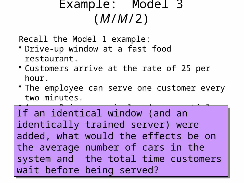
Example: Model 3 (M/M/2)
Recall the Model 1 example:• Drive-up window at a fast food restaurant.• Customers arrive at the rate of 25 per hour.• The employee can serve one customer every two
minutes.• Assume Poisson arrival and exponential service
rates.
If an identical window (and an identically trained server) were added, what would the effects be on the average number of cars in the system and the total time customers wait before being served?
If an identical window (and an identically trained server) were added, what would the effects be on the average number of cars in the system and the total time customers wait before being served?
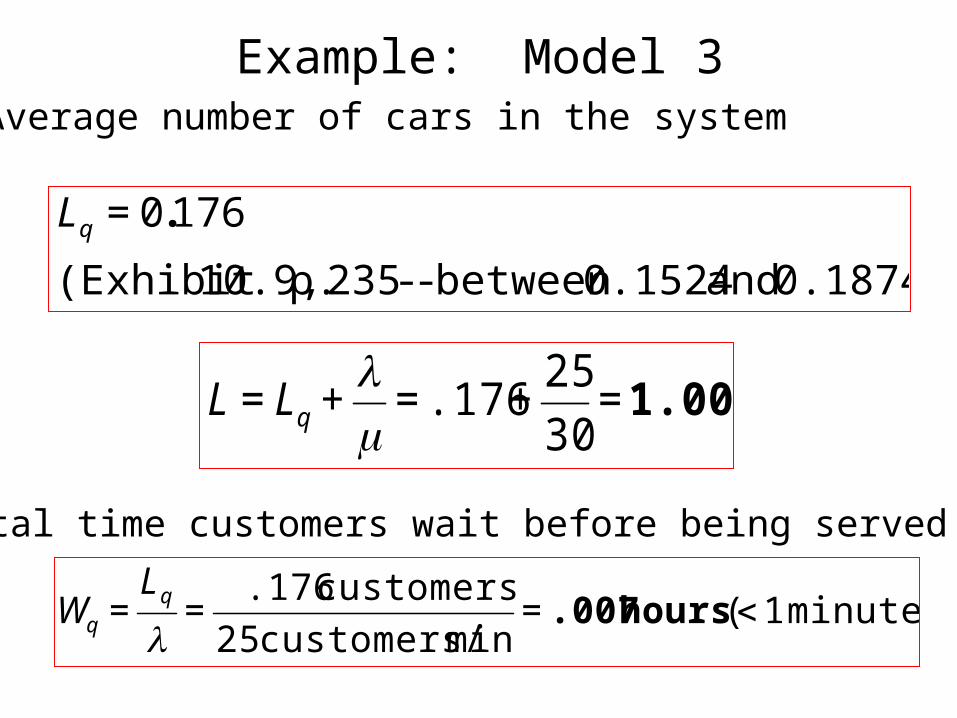
Example: Model 3Average number of cars in the system
0.1874) and 0.1524between --235 p. 10.9,(Exhibit
1760= .qL
1.009 = 3025 + .176 = + =
qLL
Total time customers wait before being served
minute) 1 ( = mincustomers/ 25
customers .176 = = hours .007
qL
qW

Operations -- Prof. Juran 53
M/M/s Calculator (Mms.xls)
1234
5
6789101112131415161718192021222324252627
A B C D E F G Hmms.xls M/M/s Queueing Formula Spreadsheet
Inputs: Definitions of terms:
lambda 25 lambda = arrival rate
mu 30 mu = service rates = number of serversLq = average number in the queueL = average number in the systemWq = average wait in the queueW = average wait in the systemP(0) = probability of zero customers in the systemP(delay) = probability that an arriving customer has to wait
Outputs:s Lq L Wq W P(0) P(delay) Utilization
01 4.1667 5.0000 0.1667 0.2000 0.1667 0.8333 0.83332 0.1751 1.0084 0.0070 0.0403 0.4118 0.2451 0.41673 0.0222 0.8555 0.0009 0.0342 0.4321 0.0577 0.27784 0.0029 0.8362 0.0001 0.0334 0.4343 0.0110 0.20835 0.0003 0.8337 0.0000 0.0333 0.4346 0.0017 0.16676 0.0000 0.8334 0.0000 0.0333 0.4346 0.0002 0.13897 0.0000 0.8333 0.0000 0.0333 0.4346 0.0000 0.11908 0.0000 0.8333 0.0000 0.0333 0.4346 0.0000 0.10429 0.0000 0.8333 0.0000 0.0333 0.4346 0.0000 0.0926
10 0.0000 0.8333 0.0000 0.0333 0.4346 0.0000 0.0833

Operations -- Prof. Juran 54
Finite Queuing: Model 4
Finite Notation:
D = Probability that an arrival must wait in line
F = Efficiency factor, a measure of the effect of having to wait in line
Ls = Average number of units being served
J = Source population less those being served
Lq = Average number of units in line
S = Number of servers

Operations -- Prof. Juran 55
n = Number of customers in the system
N = Number of customers in the source population
P = Probability of exactly n customers in the system
T = Average time to perform service
U = Average time between service (per customer)
W = Average waiting time in line
X = Service factor = UTT
(the proportion of time a customer is in service)

The copy center of an electronics firm has four copy machines that are all serviced by a single technician.
Every two hours, on average, the machines require adjustment. The technician spends an average of 10 minutes per machine when adjustment is required.
Assuming Poisson arrivals and exponential service, how many machines are “down” (on average)?
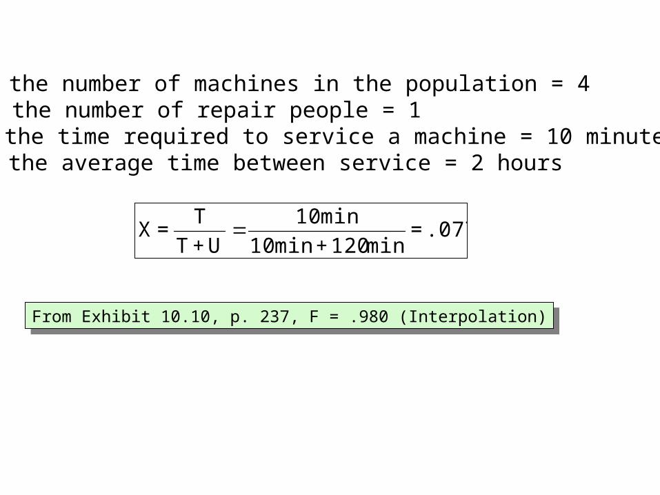
N, the number of machines in the population = 4M, the number of repair people = 1T, the time required to service a machine = 10 minutesU, the average time between service = 2 hours
.077 =min 120+min 10
min 10U+T
T=X
From Exhibit 10.10, p. 237, F = .980 (Interpolation)From Exhibit 10.10, p. 237, F = .980 (Interpolation)

Operations -- Prof. Juran 58
Lq = N(1 - F) = 4(1 - 0.980) = 0.08 machines
(From Table TN6.11: F = 0.980 , using interpolation)
Ls = FNX = 0.980(4)(0.077) = 0.302
Average number of machines down = Lq + Ls = 0.382 machines
Note: book uses L instead of Lq, and H instead of Ls

Operations -- Prof. Juran 59
Example: Airport SecurityEach airline passenger and his or her luggage must be checked to determine whether he or she is carrying weapons onto the airplane. Suppose that at Gotham City Airport, an average of 10 passengers per minute arrive, where interarrival times are exponentially distributed. To check passengers for weapons, the airport must have a checkpoint consisting of a metal detector and baggage X-ray machine.
Whenever a checkpoint is in operation, two employees are required. These two employees work simultaneously to check a single passenger. A checkpoint can check an average of 12 passengers per minute, where the time to check a passenger is also exponentially distributed.
Operations -- Prof. Juran 60
Why is an M/M/l, not an M/M/2, model relevant here?

Operations -- Prof. Juran 61
What is the probability that a passenger will have to wait before being checked for weapons?

Operations -- Prof. Juran 62
On average, how many passengers are waiting in line to enter the checkpoint?

Operations -- Prof. Juran 63
On average, how long will a passenger spend at the checkpoint (including waiting time in line)?
Operations -- Prof. Juran 64
Difficulties with Analytical Queueing Models
• Using expected values, we can get some results
• Easy to set up in a spreadsheet• It is dangerous to replace a random
variable with its expected value• Analytical methods (beyond expected
values) require difficult mathematics, and must be based on strict (perhaps unreasonable) assumptions

Operations -- Prof. Juran 65
Summary• Basic definitions and metrics• Examples of some theoretical models

![lecture16-IP-switching...What do we know so far [1] … • Network performance metrics • Transmission delay, propagation delay, queueing delay, bandwidth • Sharing networks •](https://static.documents.pub/doc/80x56/5e9e91272561997647659170/lecture16-ip-switching-what-do-we-know-so-far-1-a-network-performance-metrics.jpg)


