58
Introduction to Management Science (8th Edition, Bernard W. Taylor III) Chapter 15 Chapter 15 - Queuing Analysis 1 Queuing Analysis
Introduction to Management Science
(8th Edition, Bernard W. Taylor III)
Chapter 15
Chapter 15 - Queuing Analysis 1
Queuing Analysis
Elements of Waiting Line Analysis
The Single-Server Waiting Line System
Undefined and Constant Service Times
Chapter Topics
Undefined and Constant Service Times
Finite Queue Length
Finite Calling Problem
The Multiple-Server Waiting Line
Addition Types of Queuing Systems
Chapter 15 - Queuing Analysis 2
Significant amount of time spent in waiting lines by people, products, etc.
Providing quick service is an important aspect of quality
Overview
Providing quick service is an important aspect of quality customer service.
The basis of waiting line analysis is the trade-off between the cost of improving service and the costs associated with making customers wait.
Queuing analysis is a probabilistic form of analysis.
Chapter 15 - Queuing Analysis 3
The results are referred to as operating characteristics.
Results are used by managers of queuing operations to make decisions.
Waiting lines form because people or things arrive at a service faster than they can be served.
Most operations have sufficient server capacity to handle
Elements of Waiting Line Analysis
Most operations have sufficient server capacity to handle customers in the long run.
Customers however, do not arrive at a constant rate nor are they served in an equal amount of time.
Waiting lines are continually increasing and decreasing in length.and approach an average rate of customer arrivals and an average service time, in the long run.
Chapter 15 - Queuing Analysis 4
average service time, in the long run.
Decisions concerning the management of waiting lines are based on these averages for customer arrivals and service times.
They are used in formulas to compute operating characteristics of the system which in turn form the basis of decision making.
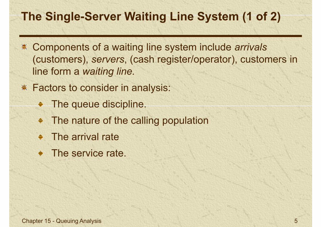
Components of a waiting line system include arrivals (customers), servers, (cash register/operator), customers in line form a waiting line.
The Single-Server Waiting Line System (1 of 2)
line form a waiting line.
Factors to consider in analysis:
The queue discipline.
The nature of the calling population
The arrival rate
The service rate.
Chapter 15 - Queuing Analysis 5
The service rate.
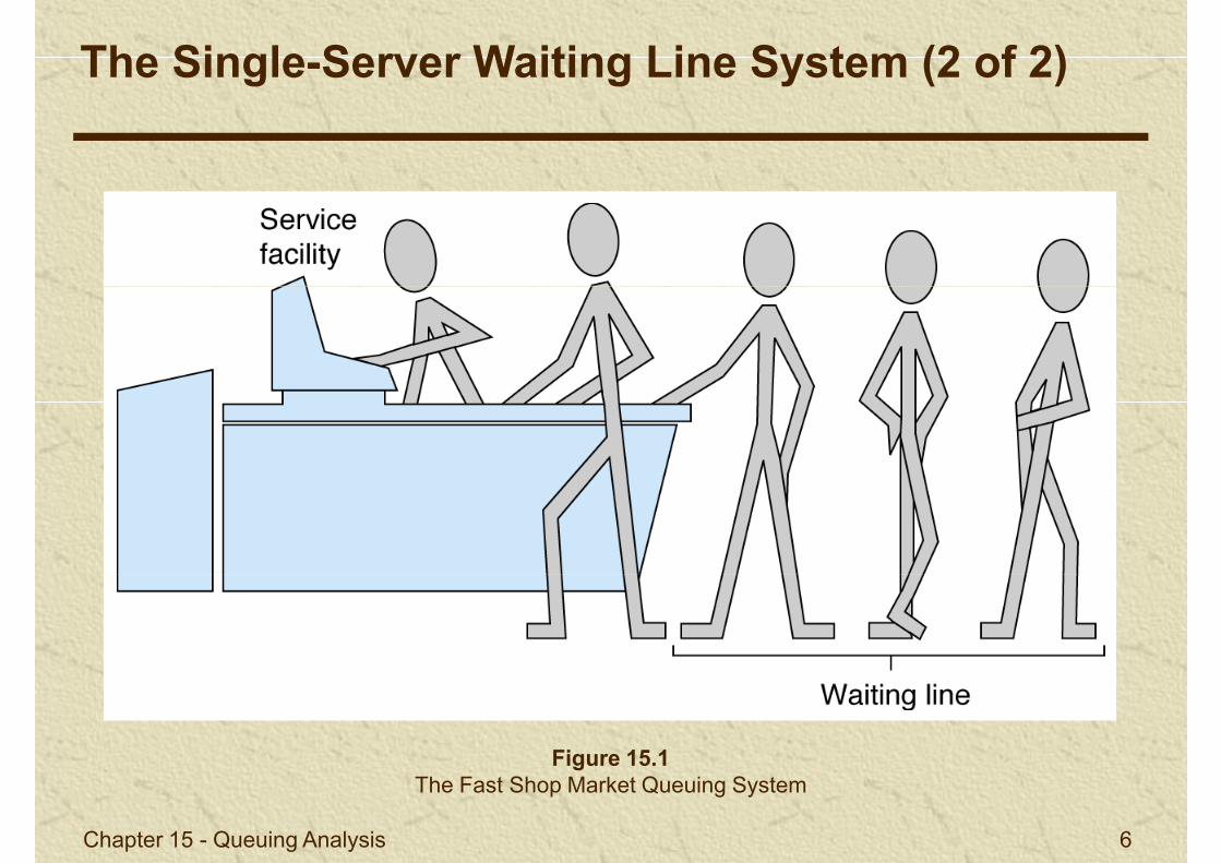
The Single-Server Waiting Line System (2 of 2)
Chapter 15 - Queuing Analysis 6
Figure 15.1The Fast Shop Market Queuing System
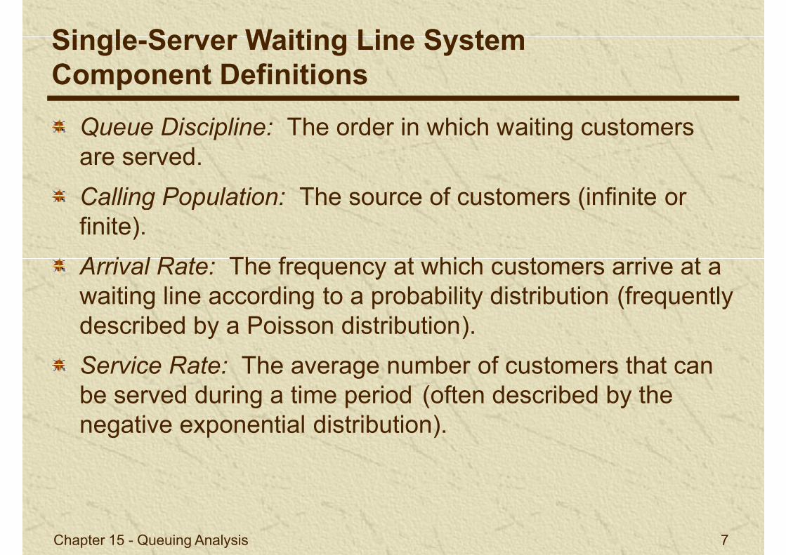
Queue Discipline: The order in which waiting customers are served.
Calling Population: The source of customers (infinite or
Single-Server Waiting Line SystemComponent Definitions
Calling Population: The source of customers (infinite or finite).
Arrival Rate: The frequency at which customers arrive at a waiting line according to a probability distribution (frequently described by a Poisson distribution).
Service Rate: The average number of customers that can
Chapter 15 - Queuing Analysis 7
Service Rate: The average number of customers that can be served during a time period (often described by the negative exponential distribution).

Assumptions of the basic single-server model:
An infinite calling population
Single-Server Waiting Line SystemSingle-Server Model
A first-come, first-served queue discipline
Poisson arrival rate
Exponential service times
Symbology:
= the arrival rate (average number of arrivals/time period)
Chapter 15 - Queuing Analysis 8
= the arrival rate (average number of arrivals/time period)
= the service rate (average number served/time period)
Customers must be served faster than they arrive ( < ) or an infinitely large queue will build up.
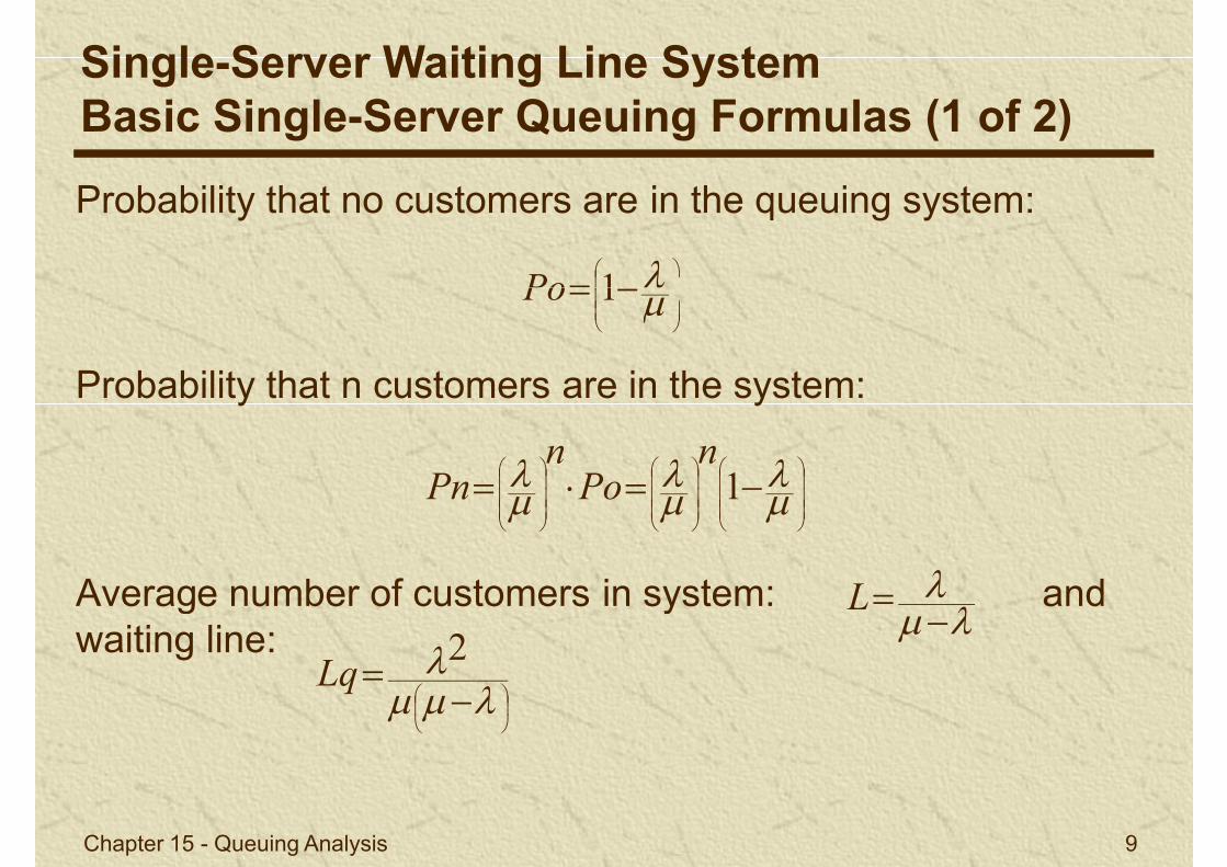
Probability that no customers are in the queuing system:
1Po
Single-Server Waiting Line SystemBasic Single-Server Queuing Formulas (1 of 2)
Probability that n customers are in the system:
Average number of customers in system: and
1Po
1
nPo
nPn
L
Chapter 15 - Queuing Analysis 9
Average number of customers in system: and waiting line:
2
Lq
L

Average time customer spends waiting and being served:
LW
1
Single-Server Waiting Line SystemBasic Single-Server Queuing Formulas (2 of 2)
Average time customer spends waiting in the queue:
Probability that server is busy (utilization factor):
LW
1
Wq
U
Chapter 15 - Queuing Analysis 10
Probability that server is idle:
11 UI
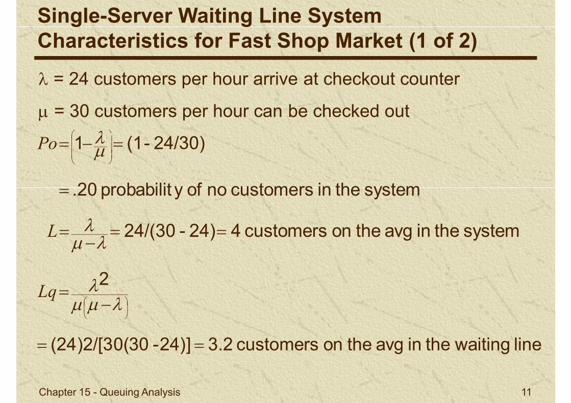
= 24 customers per hour arrive at checkout counter
= 30 customers per hour can be checked out
24/30)-(11 Po
Single-Server Waiting Line SystemCharacteristics for Fast Shop Market (1 of 2)
systemtheincustomersnoofy probabilit.20
24/30)-(11
Po
systemtheinavgtheoncustomers424)-24/(30
L
Chapter 15 - Queuing Analysis 11
line waitingtheinavgtheoncustomers3.224)]-30(24)2/[30(
2
Lq
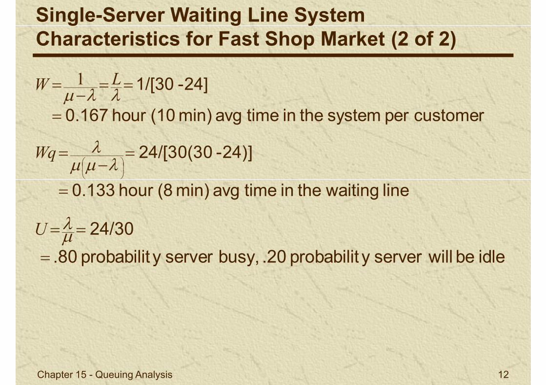
Single-Server Waiting Line SystemCharacteristics for Fast Shop Market (2 of 2)
customerpersystemtheintimeavgmin)(10hour0.167
24]-1/[30
LW 1
line waitingtheintimeavgmin)(8hour0.133
24)]-24/[30(30
Wq
idlebe willservery probabilit.20busy,servery probabilit.80
24/30
U
Chapter 15 - Queuing Analysis 12
idlebe willservery probabilit.20busy,servery probabilit.80
Single-Server Waiting Line SystemSteady-State Operating Characteristics
Because of steady-state nature of operating characteristics:
Utilization factor, U, must be less than one: U < 1,or / < 1 and < . / < 1 and < .
The ratio of the arrival rate to the service rate must be less than one or, the service rate must be greater than the arrival rate.
The server must be able to serve customers faster than the arrival rate in the long run, or waiting line will grow to infinite size.
Chapter 15 - Queuing Analysis 13
to infinite size.
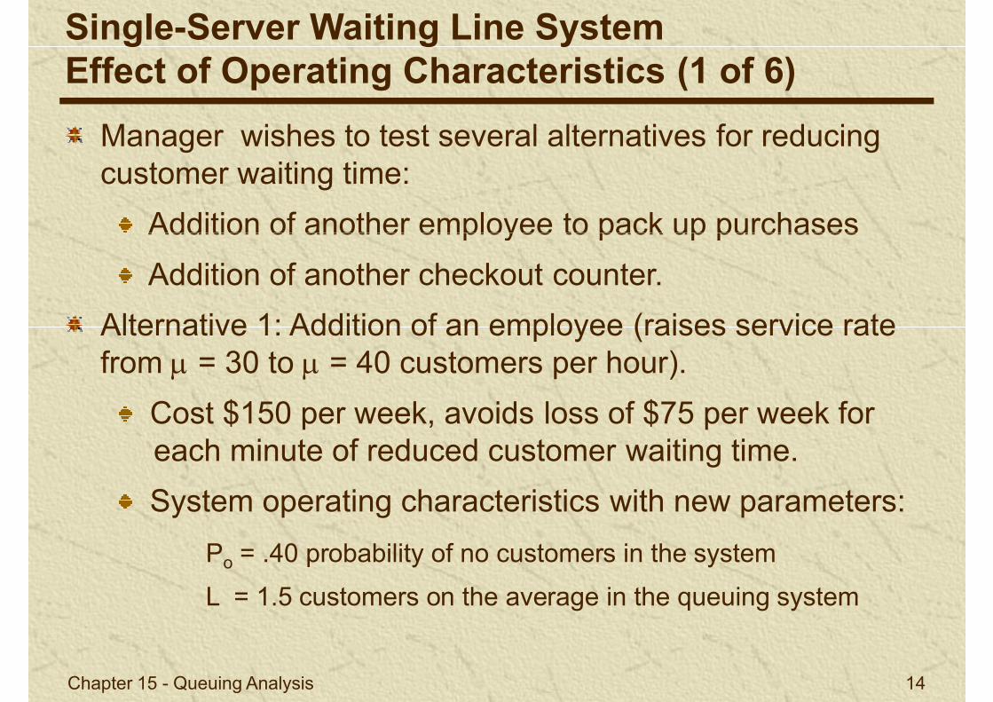
Manager wishes to test several alternatives for reducing customer waiting time:
Addition of another employee to pack up purchases
Single-Server Waiting Line SystemEffect of Operating Characteristics (1 of 6)
Addition of another employee to pack up purchases
Addition of another checkout counter.
Alternative 1: Addition of an employee (raises service rate from = 30 to = 40 customers per hour).
Cost $150 per week, avoids loss of $75 per week for each minute of reduced customer waiting time.
Chapter 15 - Queuing Analysis 14
System operating characteristics with new parameters:
Po = .40 probability of no customers in the system
L = 1.5 customers on the average in the queuing system
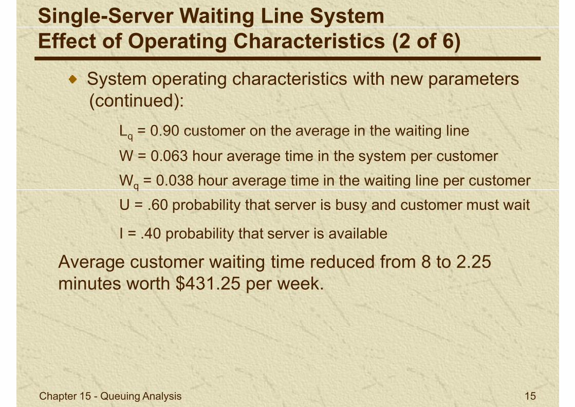
System operating characteristics with new parameters (continued):
Lq = 0.90 customer on the average in the waiting line
Single-Server Waiting Line SystemEffect of Operating Characteristics (2 of 6)
Lq = 0.90 customer on the average in the waiting line
W = 0.063 hour average time in the system per customer
Wq = 0.038 hour average time in the waiting line per customer
U = .60 probability that server is busy and customer must wait
I = .40 probability that server is available
Average customer waiting time reduced from 8 to 2.25
Chapter 15 - Queuing Analysis 15
Average customer waiting time reduced from 8 to 2.25 minutes worth $431.25 per week.
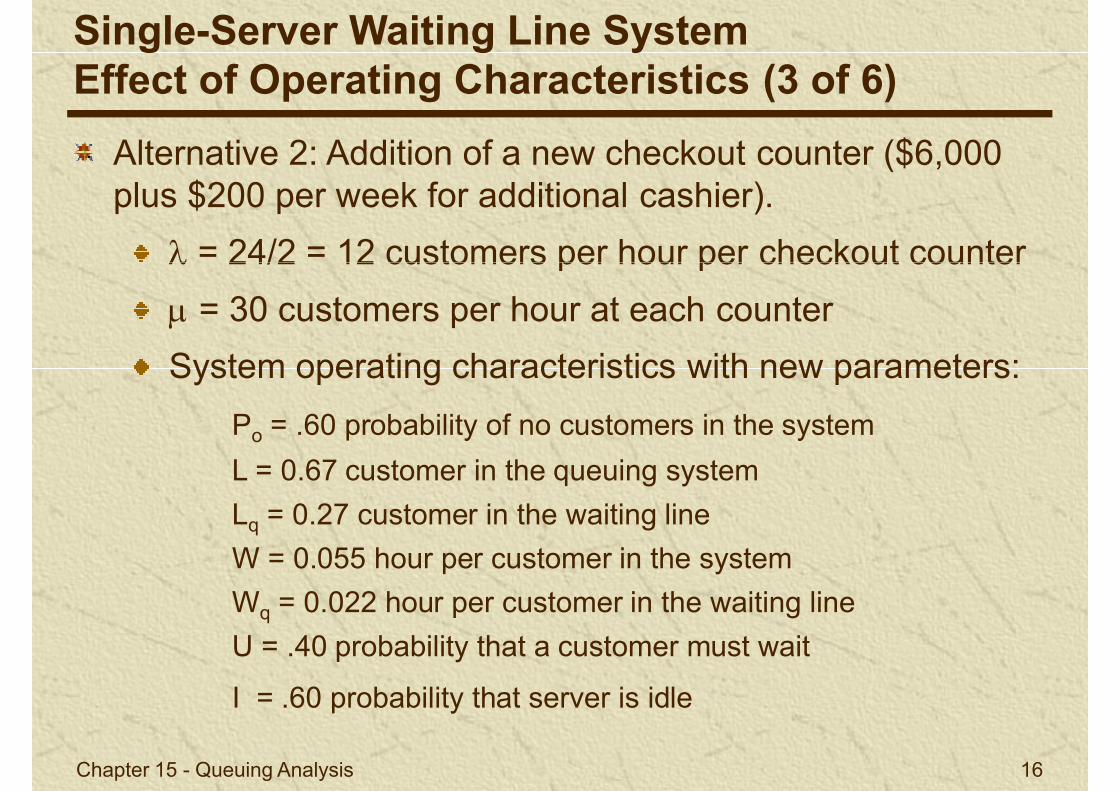
Alternative 2: Addition of a new checkout counter ($6,000 plus $200 per week for additional cashier).
= 24/2 = 12 customers per hour per checkout counter
Single-Server Waiting Line SystemEffect of Operating Characteristics (3 of 6)
= 24/2 = 12 customers per hour per checkout counter
= 30 customers per hour at each counter
System operating characteristics with new parameters:
Po = .60 probability of no customers in the system
L = 0.67 customer in the queuing system
Lq = 0.27 customer in the waiting line
Chapter 15 - Queuing Analysis 16
Lq = 0.27 customer in the waiting line
W = 0.055 hour per customer in the system
Wq = 0.022 hour per customer in the waiting line
U = .40 probability that a customer must wait
I = .60 probability that server is idle
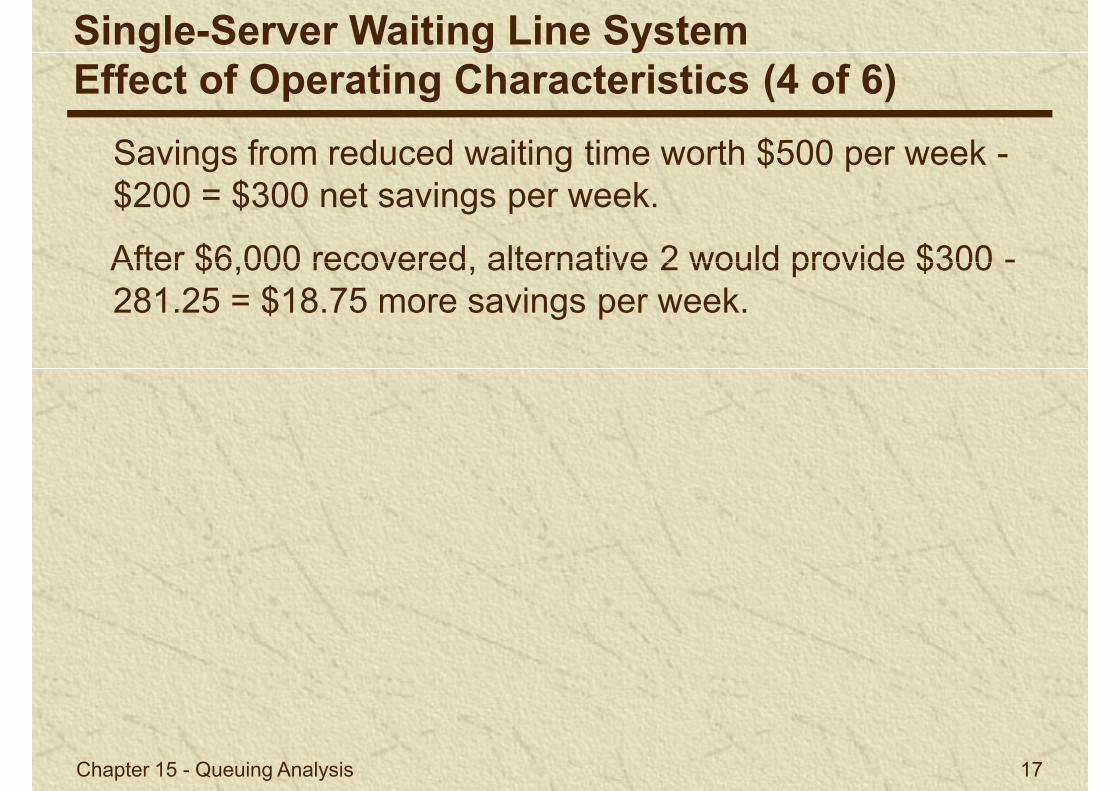
Savings from reduced waiting time worth $500 per week -$200 = $300 net savings per week.
After $6,000 recovered, alternative 2 would provide $300 -
Single-Server Waiting Line SystemEffect of Operating Characteristics (4 of 6)
After $6,000 recovered, alternative 2 would provide $300 -281.25 = $18.75 more savings per week.
Chapter 15 - Queuing Analysis 17
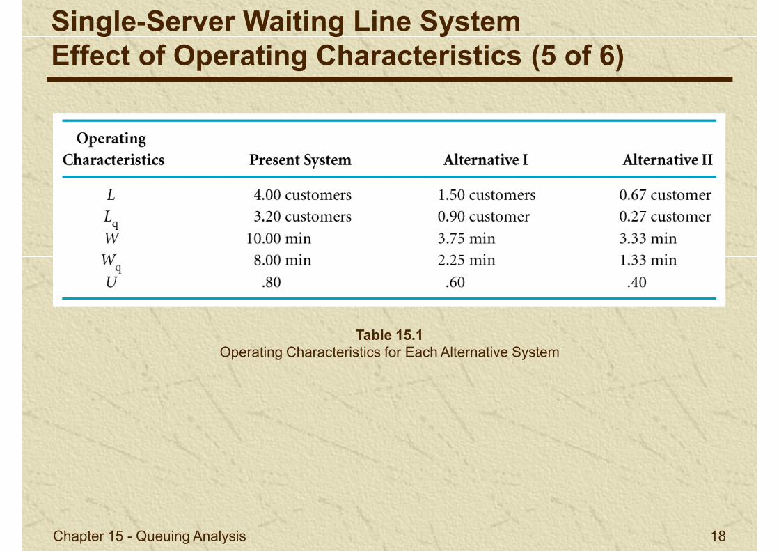
Single-Server Waiting Line SystemEffect of Operating Characteristics (5 of 6)
Table 15.1Operating Characteristics for Each Alternative System
Chapter 15 - Queuing Analysis 18
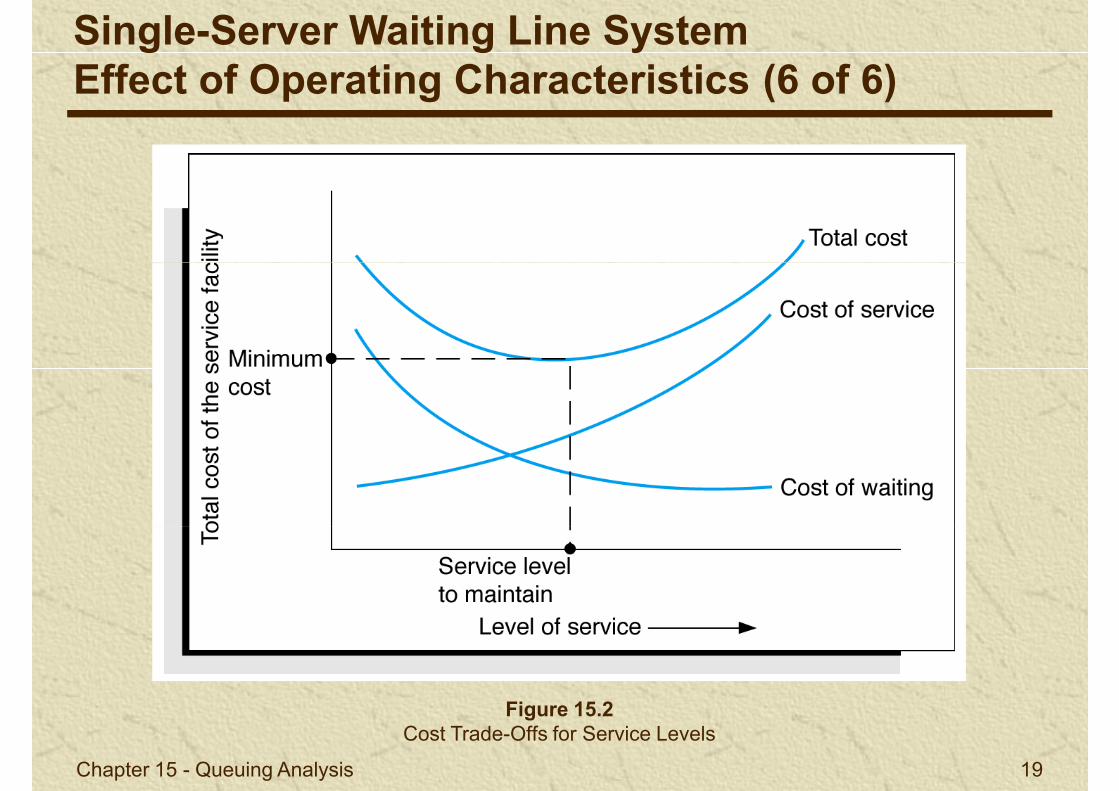
Single-Server Waiting Line SystemEffect of Operating Characteristics (6 of 6)
Chapter 15 - Queuing Analysis 19
Figure 15.2Cost Trade-Offs for Service Levels
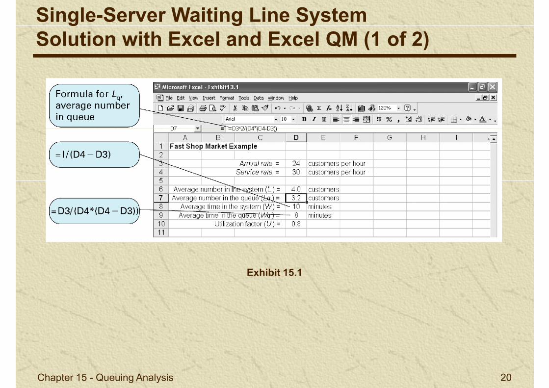
Single-Server Waiting Line SystemSolution with Excel and Excel QM (1 of 2)
Chapter 15 - Queuing Analysis 20
Exhibit 15.1

Single-Server Waiting Line SystemSolution with Excel and Excel QM (2 of 2)
Chapter 15 - Queuing Analysis 21
Exhibit 15.2

Single-Server Waiting Line SystemSolution with QM for Windows
Chapter 15 - Queuing Analysis 22
Exhibit 15.3
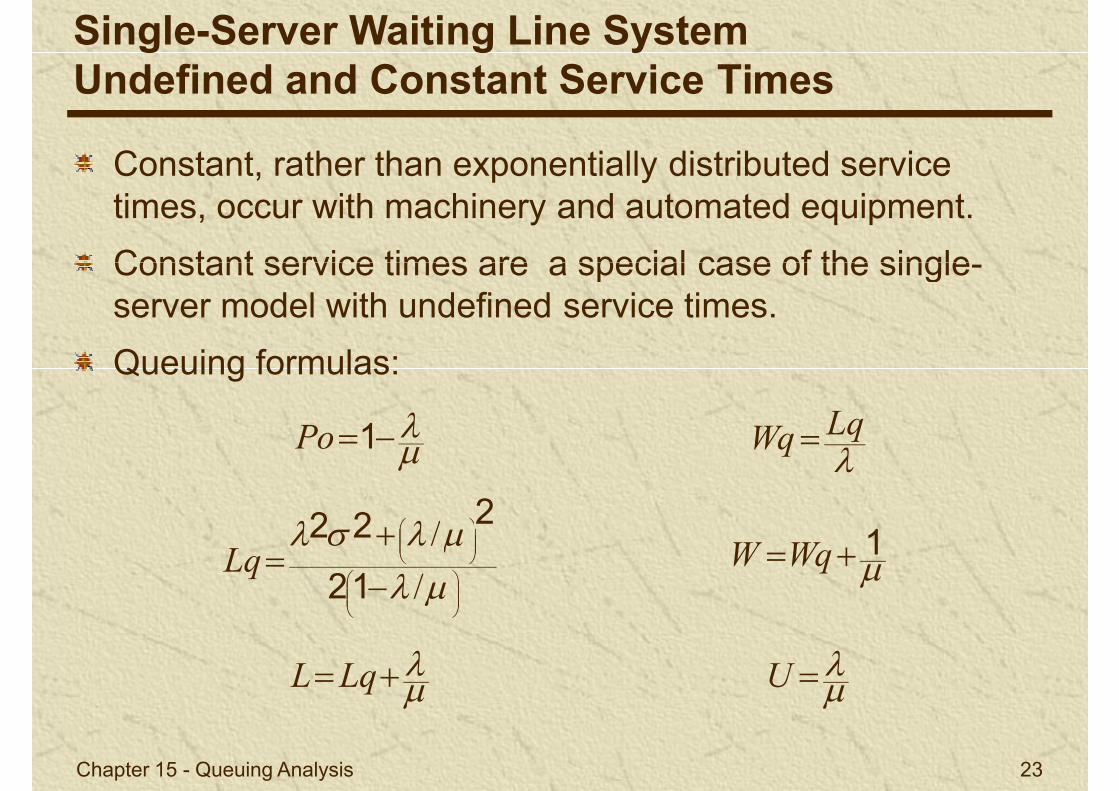
Constant, rather than exponentially distributed service times, occur with machinery and automated equipment.
Constant service times are a special case of the single-
Single-Server Waiting Line SystemUndefined and Constant Service Times
Constant service times are a special case of the single-server model with undefined service times.
Queuing formulas:
1Po
/222
LqWq
1
Chapter 15 - Queuing Analysis 23
/
/
12
222Lq
LqL
1WqW
U
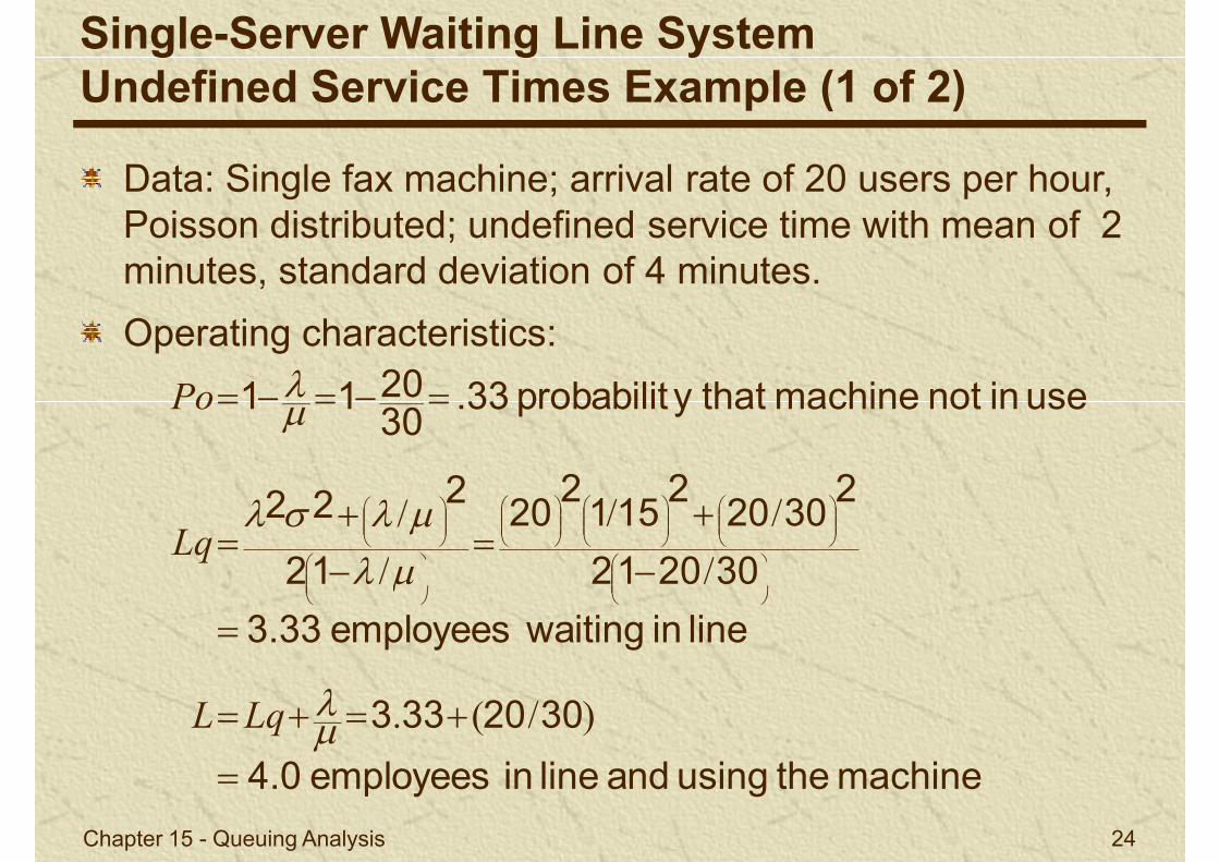
Data: Single fax machine; arrival rate of 20 users per hour, Poisson distributed; undefined service time with mean of 2 minutes, standard deviation of 4 minutes.
Single-Server Waiting Line SystemUndefined Service Times Example (1 of 2)
302012
23020
2151
220
12
222
useinnotmachinethaty probabilit.33302011
/
//
/
/
Lq
Po
minutes, standard deviation of 4 minutes.
Operating characteristics:
Chapter 15 - Queuing Analysis 24
machinetheusingandlineinemployees4.0
3020333
linein waitingemployees3.33
30201212
)/(.
//
LqL
time waitingminutes10hour1665020333
LqWq ..
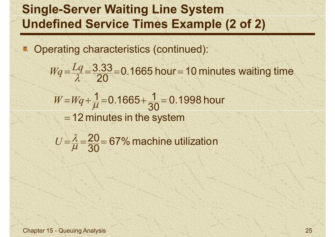
Operating characteristics (continued):
Single-Server Waiting Line SystemUndefined Service Times Example (2 of 2)
nutilizatiomachine67%3020
systemtheinminutes12
hour0.1998301166501
20
U
WqW .
Chapter 15 - Queuing Analysis 25
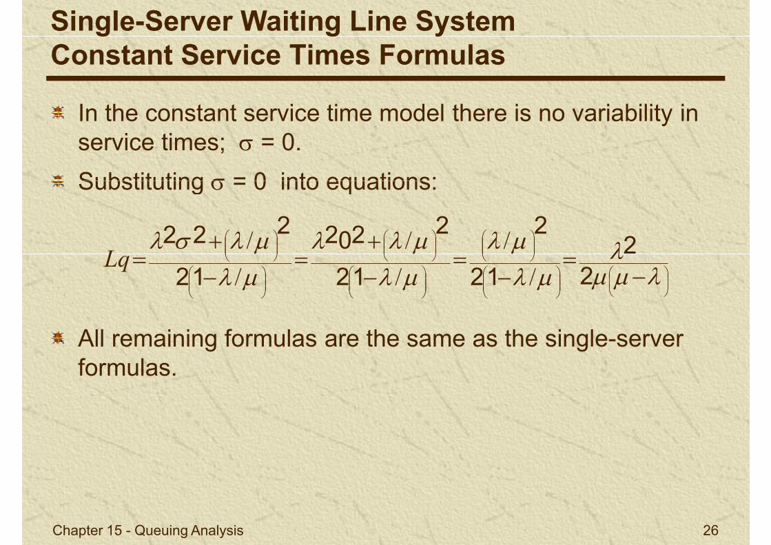
In the constant service time model there is no variability in service times; = 0.
Substituting = 0 into equations:
Single-Server Waiting Line SystemConstant Service Times Formulas
Substituting = 0 into equations:
All remaining formulas are the same as the single-server formulas.
22
12
2
12
2202
12
222
/
/
/
/
/
/Lq
Chapter 15 - Queuing Analysis 26
formulas.
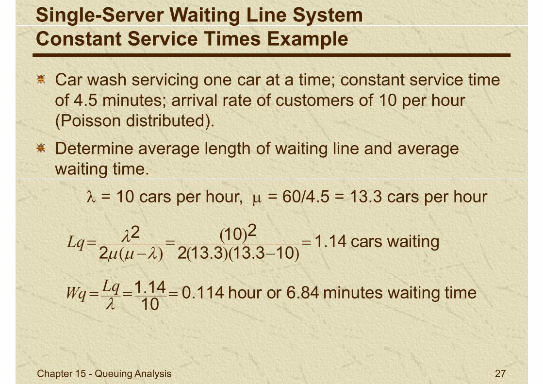
Car wash servicing one car at a time; constant service time of 4.5 minutes; arrival rate of customers of 10 per hour (Poisson distributed).
Single-Server Waiting Line SystemConstant Service Times Example
waitingcars1.14103133132
2102
2
).)(.(
)()(
Lq
(Poisson distributed).
Determine average length of waiting line and average waiting time.
= 10 cars per hour, = 60/4.5 = 13.3 cars per hour
Chapter 15 - Queuing Analysis 27
time waitingminutes6.84orhour0.11410141
1031331322
.
).)(.()(
LqWq
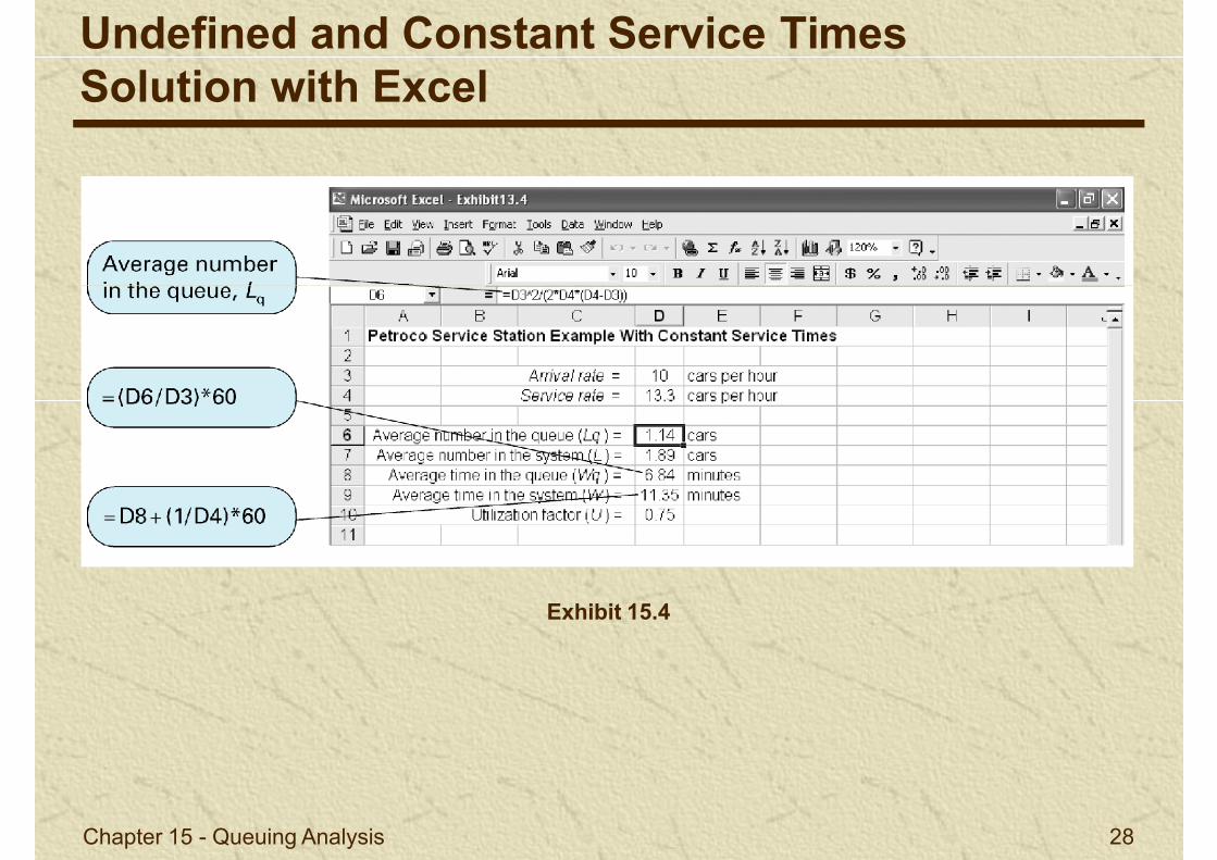
Undefined and Constant Service TimesSolution with Excel
Chapter 15 - Queuing Analysis 28
Exhibit 15.4

Undefined and Constant Service TimesSolution with QM for Windows
Exhibit 15.5
Chapter 15 - Queuing Analysis 29
Exhibit 15.5
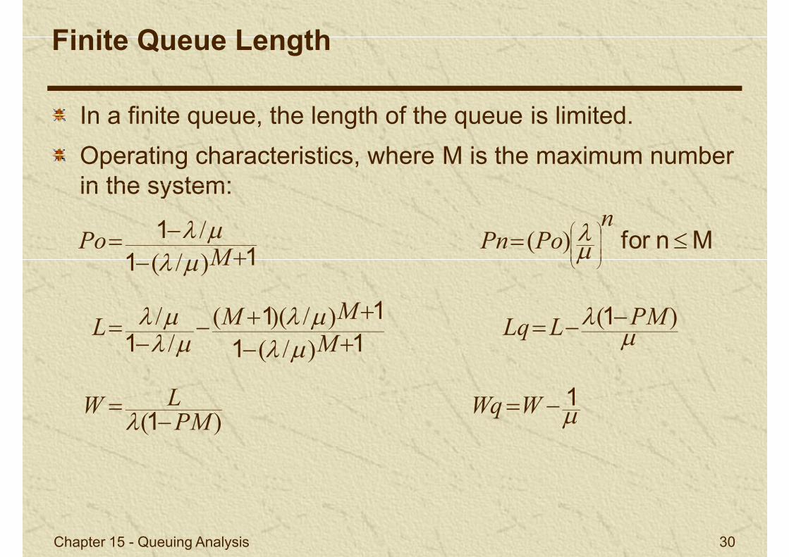
In a finite queue, the length of the queue is limited.
Operating characteristics, where M is the maximum number in the system:
Finite Queue Length
1 11
111
Mnfor 11
1
PMLLqM
MML
nPoPn
MPo
)()/(
)/)((/
/
)()/(/
in the system:
Chapter 15 - Queuing Analysis 30
1
1
WWq
PMLW
)(
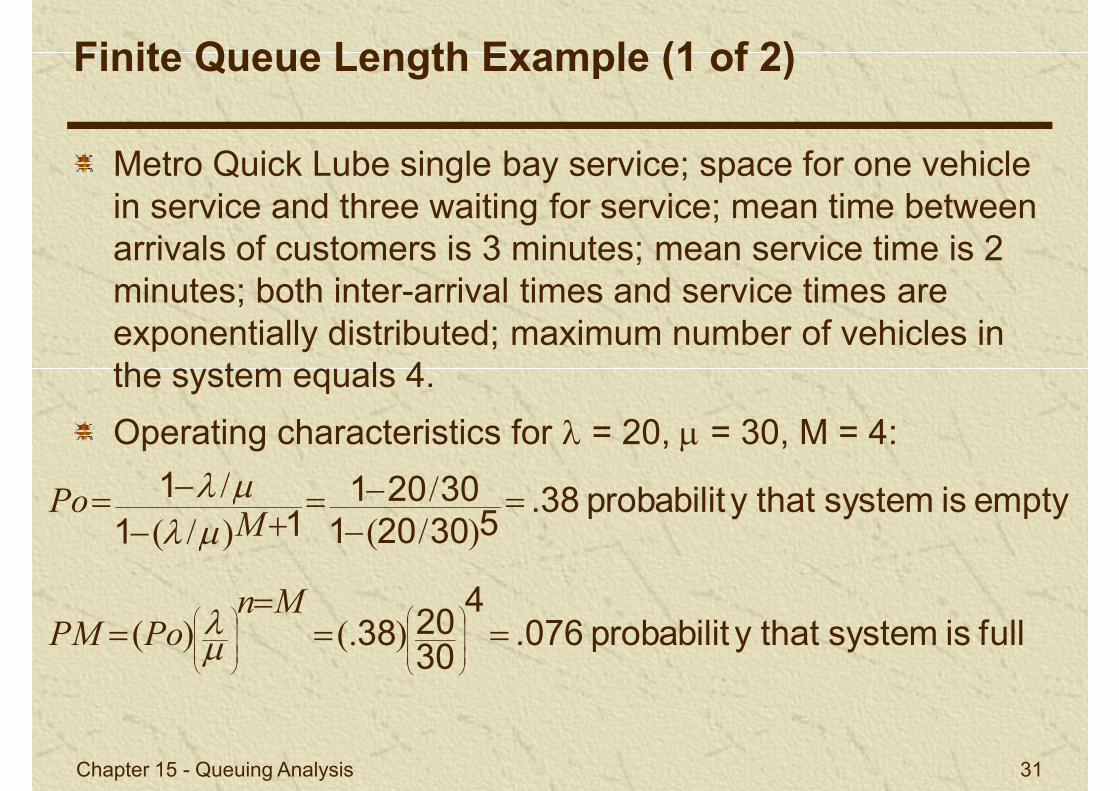
Metro Quick Lube single bay service; space for one vehicle in service and three waiting for service; mean time between arrivals of customers is 3 minutes; mean service time is 2
Finite Queue Length Example (1 of 2)
arrivals of customers is 3 minutes; mean service time is 2 minutes; both inter-arrival times and service times are exponentially distributed; maximum number of vehicles in the system equals 4.
Operating characteristics for = 20, = 30, M = 4:
emptyissystemthaty probabilit.38530201
3020111
1
)/(/
)/(/M
Po
Chapter 15 - Queuing Analysis 31
fullissystemthaty probabilit.0764
302038
53020111
)(.)(
)/()/(
MnPoPM
M
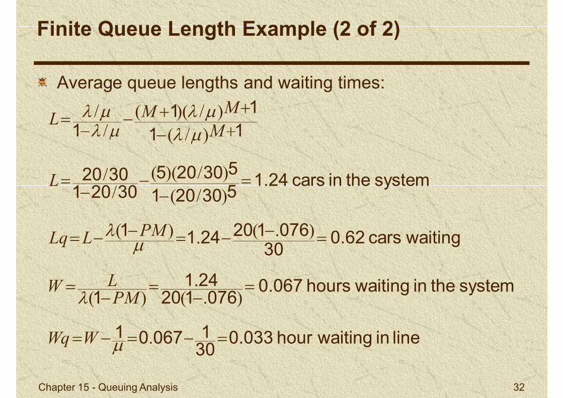
Average queue lengths and waiting times:
11
111
)/(
)/)((/
/
MMML
Finite Queue Length Example (2 of 2)
waitingcars0.6230
0761202411
systemtheincars1.24530201
53020530201
3020
111
).(.)(
)/()/)((
//
)/(/
PMLLq
L
M
Chapter 15 - Queuing Analysis 32
linein waitinghour0.03330106701
systemthein waitinghours0.067076120
2411
.
).(.
)(
WWq
PMLW
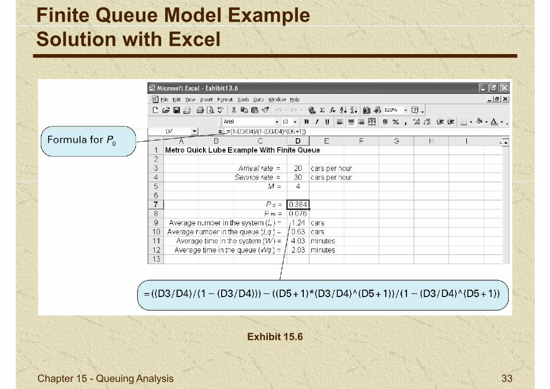
Finite Queue Model ExampleSolution with Excel
Chapter 15 - Queuing Analysis 33
Exhibit 15.6
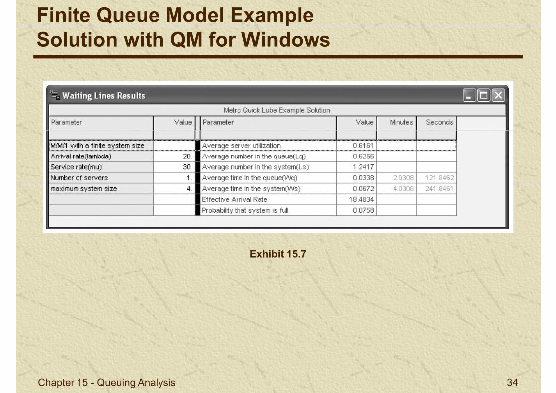
Finite Queue Model ExampleSolution with QM for Windows
Exhibit 15.7
Chapter 15 - Queuing Analysis 34
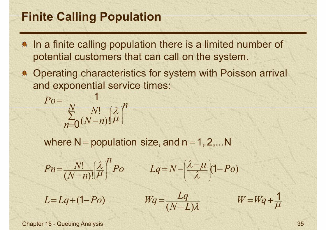
In a finite calling population there is a limited number of potential customers that can call on the system.
Operating characteristics for system with Poisson arrival
Finite Calling Population
2,...N1,nandsize,populationNwhere
0
1
nN
n nNN
Po
)!(!
Operating characteristics for system with Poisson arrival and exponential service times:
Chapter 15 - Queuing Analysis 35
1 1
1
WqWLN
LqWqPoLqL
PoNLqPon
nNNPn
)()(
)()!(
!

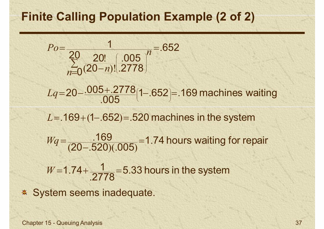
Wheelco Manufacturing Company; 20 machines; each machine operates an average of 200 hours before breaking down; average time to repair is 3.6 hours; breakdown rate is Poisson distributed, service time is exponentially
Finite Calling Population Example (1 of 2)
is Poisson distributed, service time is exponentially distributed.
Is repair staff sufficient?
= 1/200 hour = .005 per hour
= 1/3.6 hour = .2778 per hour
Chapter 15 - Queuing Analysis 36
N = 20 machines
65220
0 2778005
2020
1 .
..
)!(!
n
n
n
Po
Finite Calling Population Example (2 of 2)
repairfor waitinghours74100552020
169
systemtheinmachines5206521169
waitingmachines1696521005
277800520
0
.))(..(
.
.).(.
...
..
Wq
L
Lq
n
Chapter 15 - Queuing Analysis 37
System seems inadequate.
systemtheinhours3352778
1741
00552020
..
.
))(..(
W
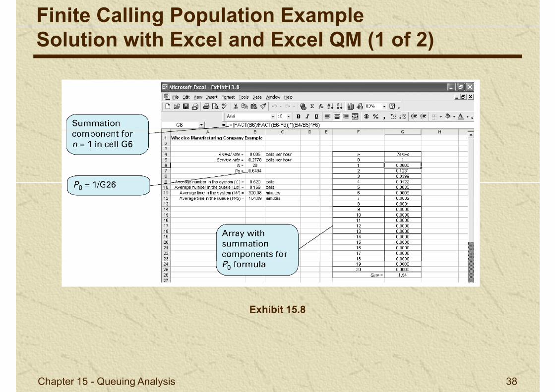
Finite Calling Population ExampleSolution with Excel and Excel QM (1 of 2)
Chapter 15 - Queuing Analysis 38
Exhibit 15.8
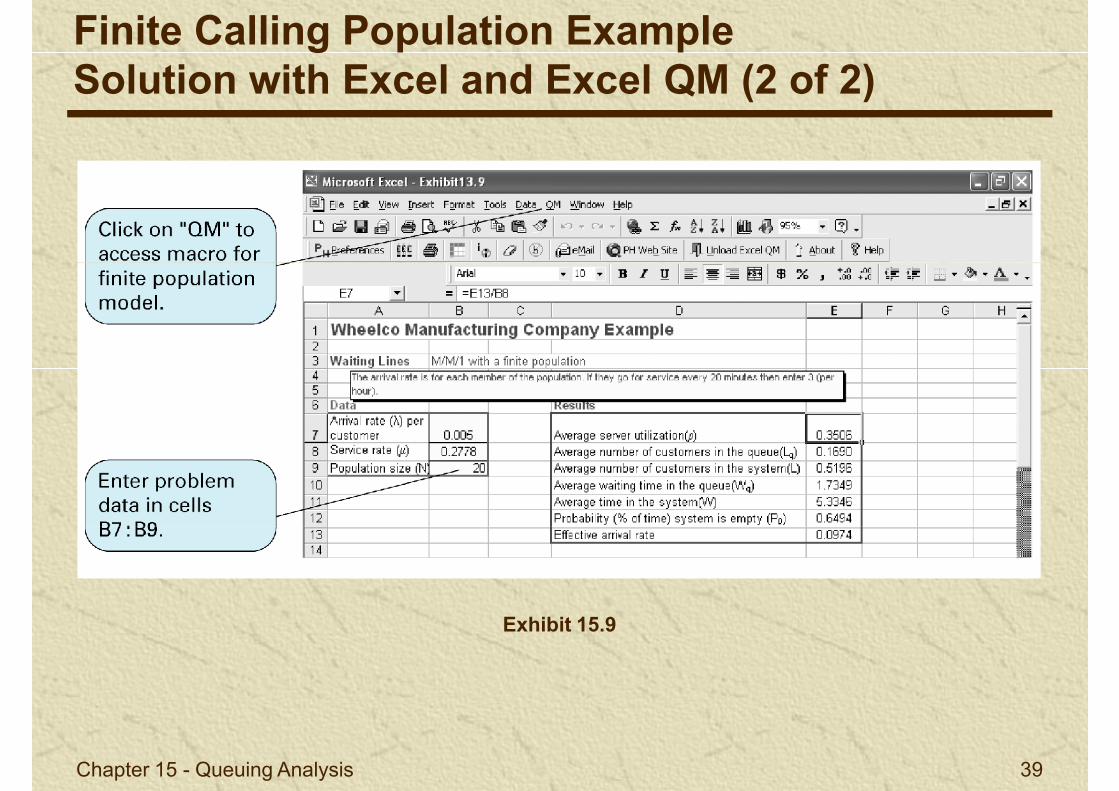
Finite Calling Population ExampleSolution with Excel and Excel QM (2 of 2)
Chapter 15 - Queuing Analysis 39
Exhibit 15.9
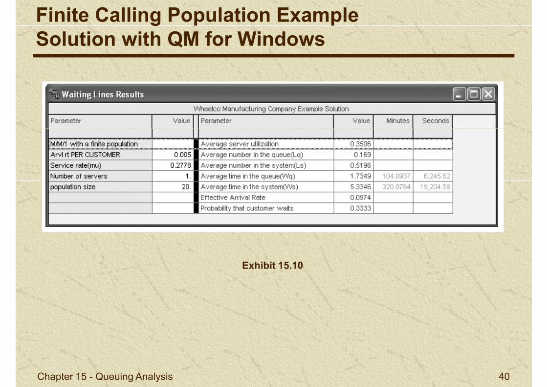
Finite Calling Population ExampleSolution with QM for Windows
Chapter 15 - Queuing Analysis 40
Exhibit 15.10

In multiple-server models, two or more independent servers in parallel serve a single waiting line.
Biggs Department Store service department; first-come,
Multiple-Server Waiting Line (1 of 2)
Biggs Department Store service department; first-come, first-served basis.
Chapter 15 - Queuing Analysis 41

Multiple-Server Waiting Line (2 of 2)
Figure 15.3Customer Service
Queuing System
Chapter 15 - Queuing Analysis 42
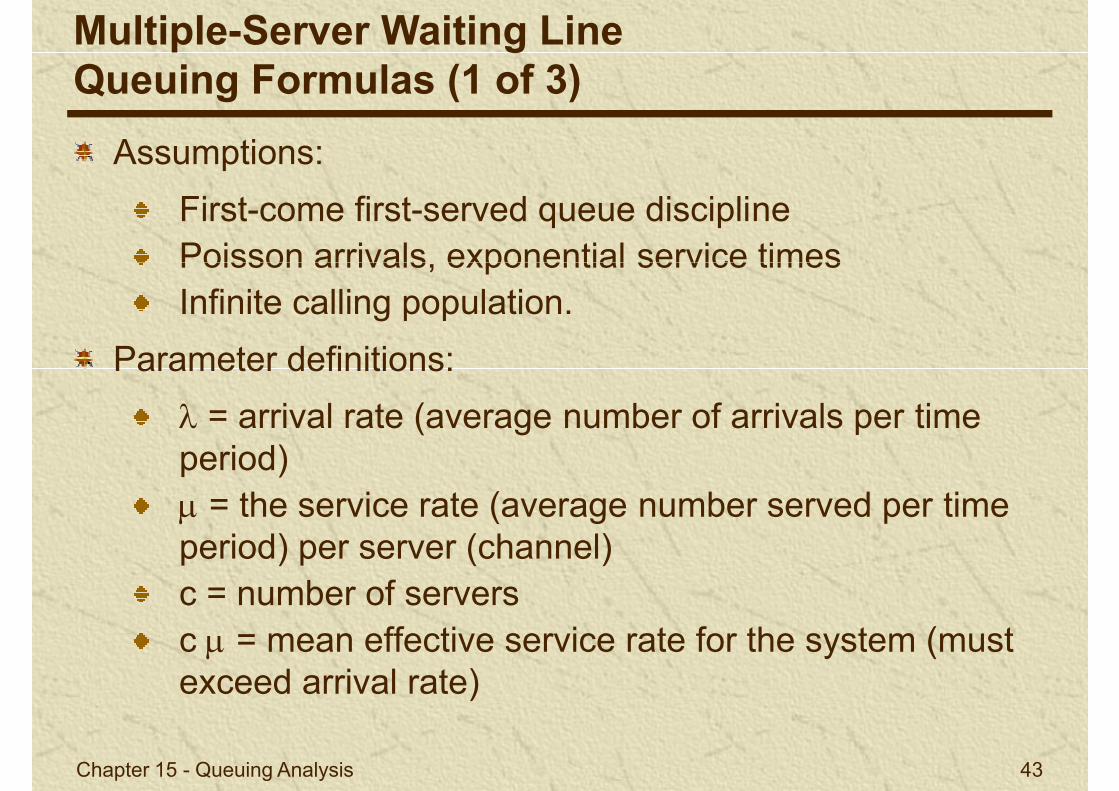
Multiple-Server Waiting LineQueuing Formulas (1 of 3)
Assumptions:
First-come first-served queue disciplinePoisson arrivals, exponential service times Poisson arrivals, exponential service times Infinite calling population.
Parameter definitions:
= arrival rate (average number of arrivals per time period) = the service rate (average number served per time
Chapter 15 - Queuing Analysis 43
period) per server (channel)c = number of serversc = mean effective service rate for the system (must exceed arrival rate)
systemincustomersnoy probabilit11
01
1
ccc
ccn
n
n
n
Po
!!
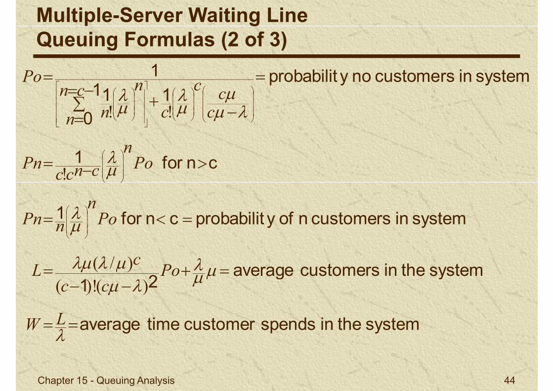
Multiple-Server Waiting LineQueuing Formulas (2 of 3)
systemtheincustomersaverage
systemincustomersnofy probabilitc nfor1
cnfor 1
Poc
L
Pon
nPn
Pon
cnccPn
)/(
!
Chapter 15 - Queuing Analysis 44
systemtheinspendscustomertimeaverage
systemtheincustomersaverage21
LW
Pocc
cL
)()!()/(
queuetheiniscustomertimeaverage1
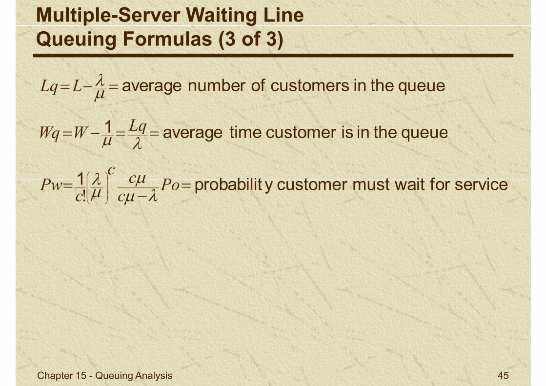
queuetheincustomersofnumberaverage
LqWWq
LLq
Multiple-Server Waiting LineQueuing Formulas (3 of 3)
servicefor waitmustcustomery probabilit1
queuetheiniscustomertimeaverage1
Po
ccc
cPw
LqWWq
!
Chapter 15 - Queuing Analysis 45
1043433
410
31
2
410
21
1
410
11
0
410
01
1
)()(
!!!!
Po
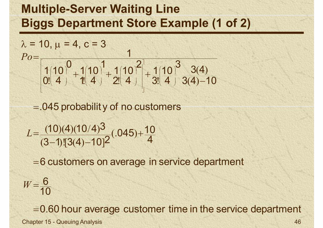
Multiple-Server Waiting LineBiggs Department Store Example (1 of 2)
= 10, = 4, c = 3
410045
2104313
3410410
customersnoofy probabilit045
1043410
31
410
21
410
11
410
01
)(.])([)!(
)/)()((
.
)(!!!!
L
Chapter 15 - Queuing Analysis 46
departmentservicetheintimecustomeraveragehour600
106
departmentserviceinaverageoncustomers6
.
W
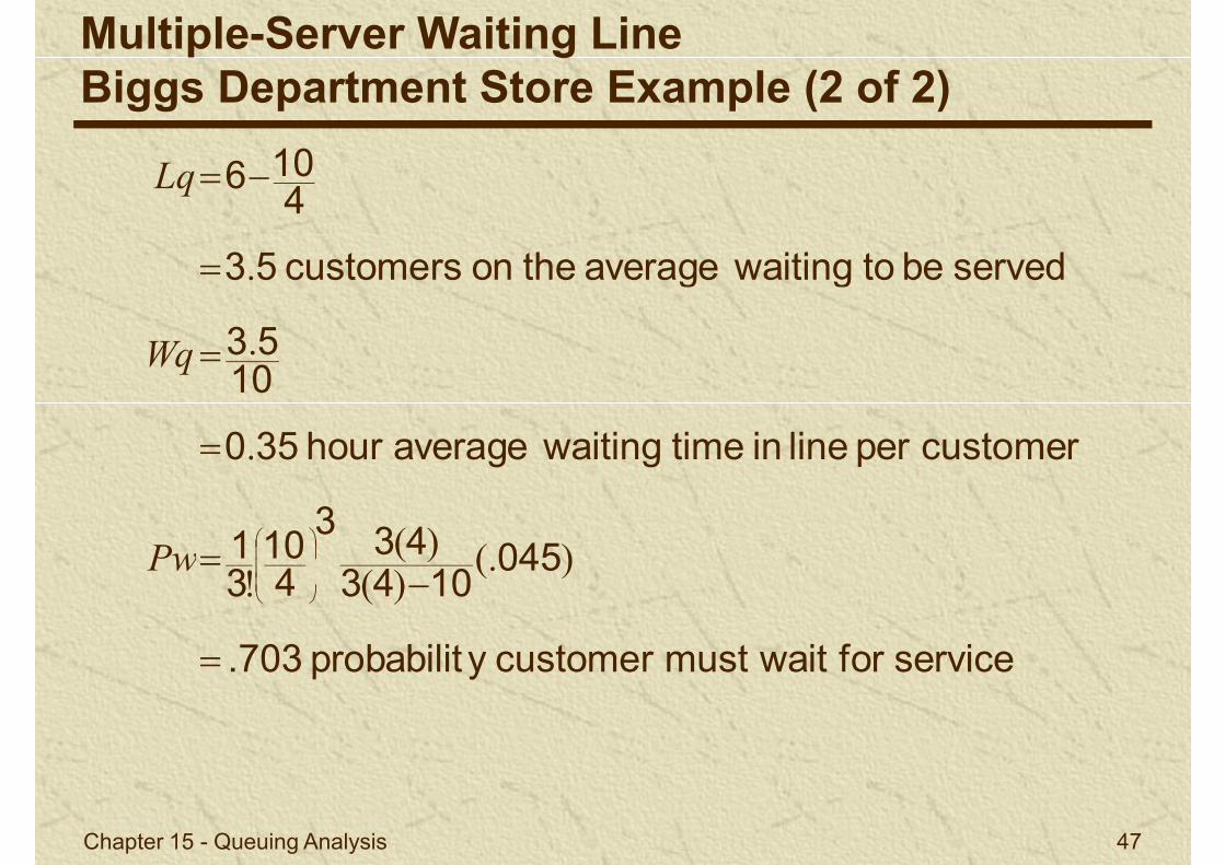
servedbeto waitingaveragetheoncustomers53
4106
.
Lq
Multiple-Server Waiting LineBiggs Department Store Example (2 of 2)
0451043
433
410
31
customerperlineintime waitingaveragehour350
1053
servedbeto waitingaveragetheoncustomers53
)(.)(
)(!
.
.
.
Pw
Wq
Chapter 15 - Queuing Analysis 47
servicefor waitmustcustomery probabilit.703
045104343
)(.)(!
Pw
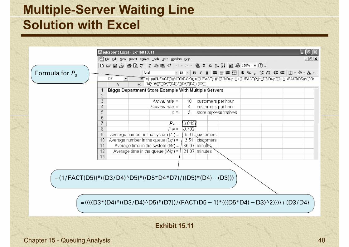
Multiple-Server Waiting LineSolution with Excel
Chapter 15 - Queuing Analysis 48
Exhibit 15.11
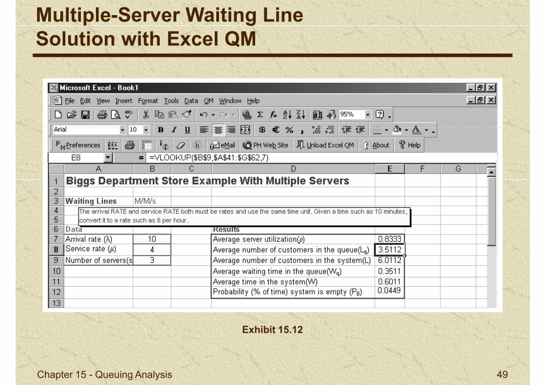
Multiple-Server Waiting LineSolution with Excel QM
Chapter 15 - Queuing Analysis 49
Exhibit 15.12
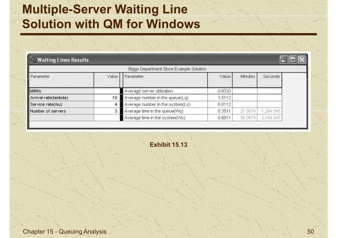
Multiple-Server Waiting LineSolution with QM for Windows
Exhibit 15.13
Chapter 15 - Queuing Analysis 50
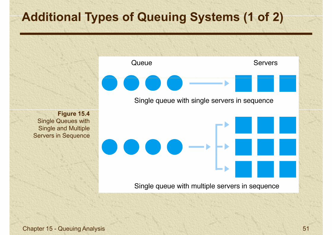
Additional Types of Queuing Systems (1 of 2)
Figure 15.4Single Queues with Single and Multiple
Servers in Sequence
Chapter 15 - Queuing Analysis 51
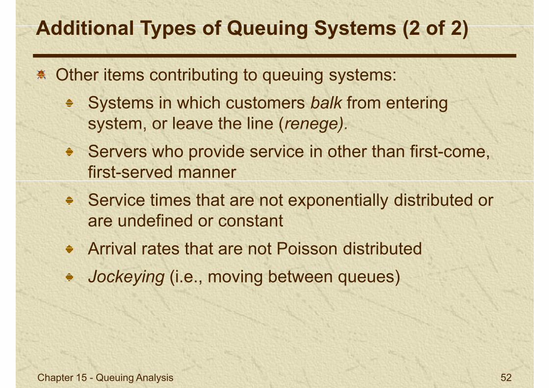
Other items contributing to queuing systems:
Systems in which customers balk from entering system, or leave the line (renege).
Additional Types of Queuing Systems (2 of 2)
system, or leave the line (renege).
Servers who provide service in other than first-come, first-served manner
Service times that are not exponentially distributed or are undefined or constant
Arrival rates that are not Poisson distributed
Chapter 15 - Queuing Analysis 52
Jockeying (i.e., moving between queues)
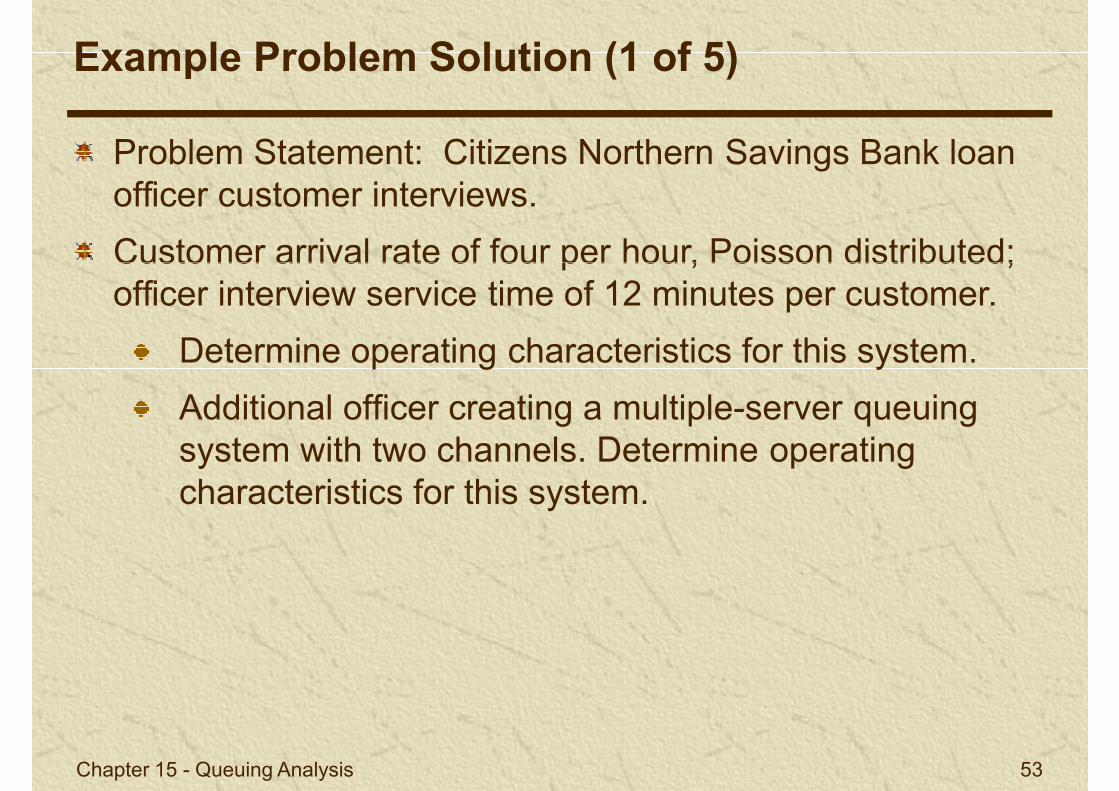
Problem Statement: Citizens Northern Savings Bank loan officer customer interviews.
Customer arrival rate of four per hour, Poisson distributed;
Example Problem Solution (1 of 5)
Customer arrival rate of four per hour, Poisson distributed; officer interview service time of 12 minutes per customer.
Determine operating characteristics for this system.
Additional officer creating a multiple-server queuing system with two channels. Determine operating characteristics for this system.
Chapter 15 - Queuing Analysis 53
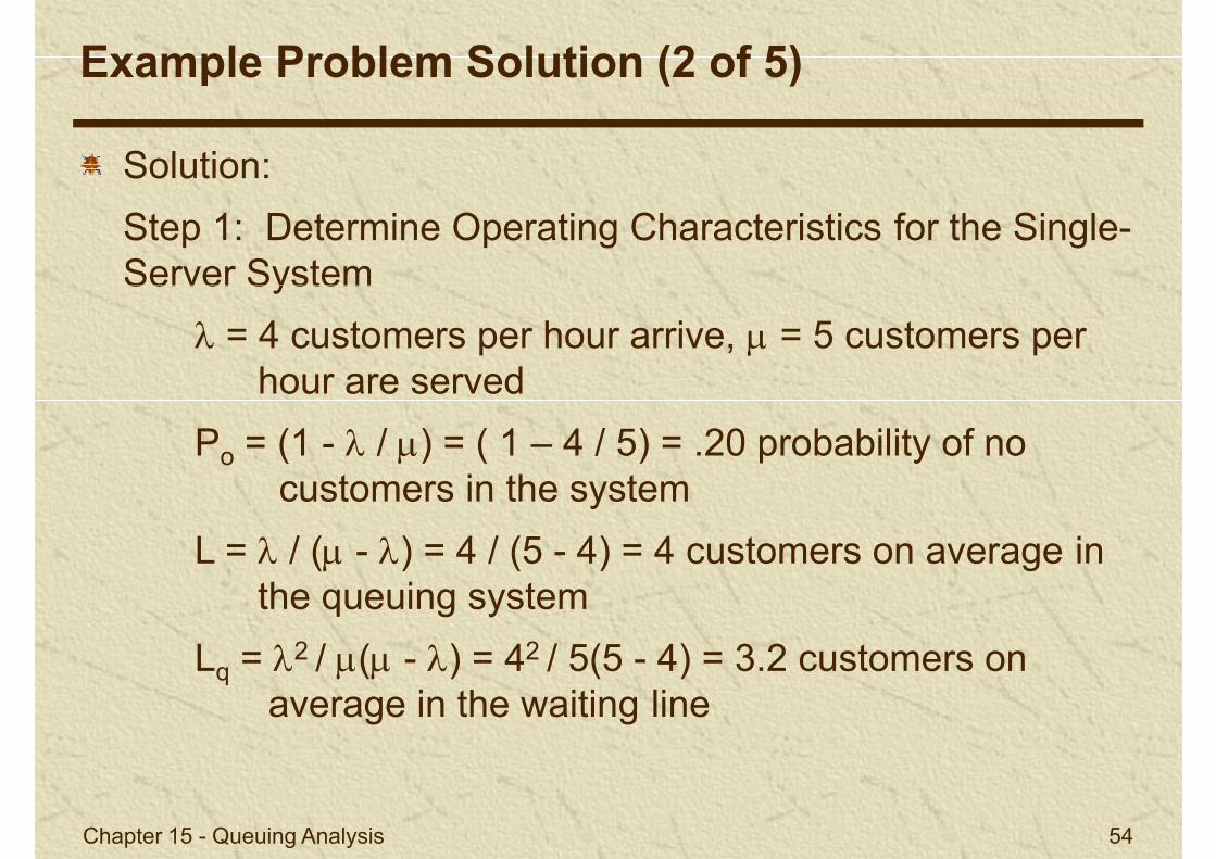
Solution:
Step 1: Determine Operating Characteristics for the Single-Server System
Example Problem Solution (2 of 5)
Server System
= 4 customers per hour arrive, = 5 customers per hour are served
Po = (1 - / ) = ( 1 – 4 / 5) = .20 probability of no customers in the system
L = / ( - ) = 4 / (5 - 4) = 4 customers on average in
Chapter 15 - Queuing Analysis 54
the queuing system
Lq = 2 / ( - ) = 42 / 5(5 - 4) = 3.2 customers on average in the waiting line

Step 1 (continued):
W = 1 / ( - ) = 1 / (5 - 4) = 1 hour on average in the system
Example Problem Solution (3 of 5)
system
Wq = / (u - ) = 4 / 5(5 - 4) = 0.80 hour (48 minutes) average time in the waiting line
Pw = / = 4 / 5 = .80 probability the new accounts officer is busy and a customer must wait
Chapter 15 - Queuing Analysis 55
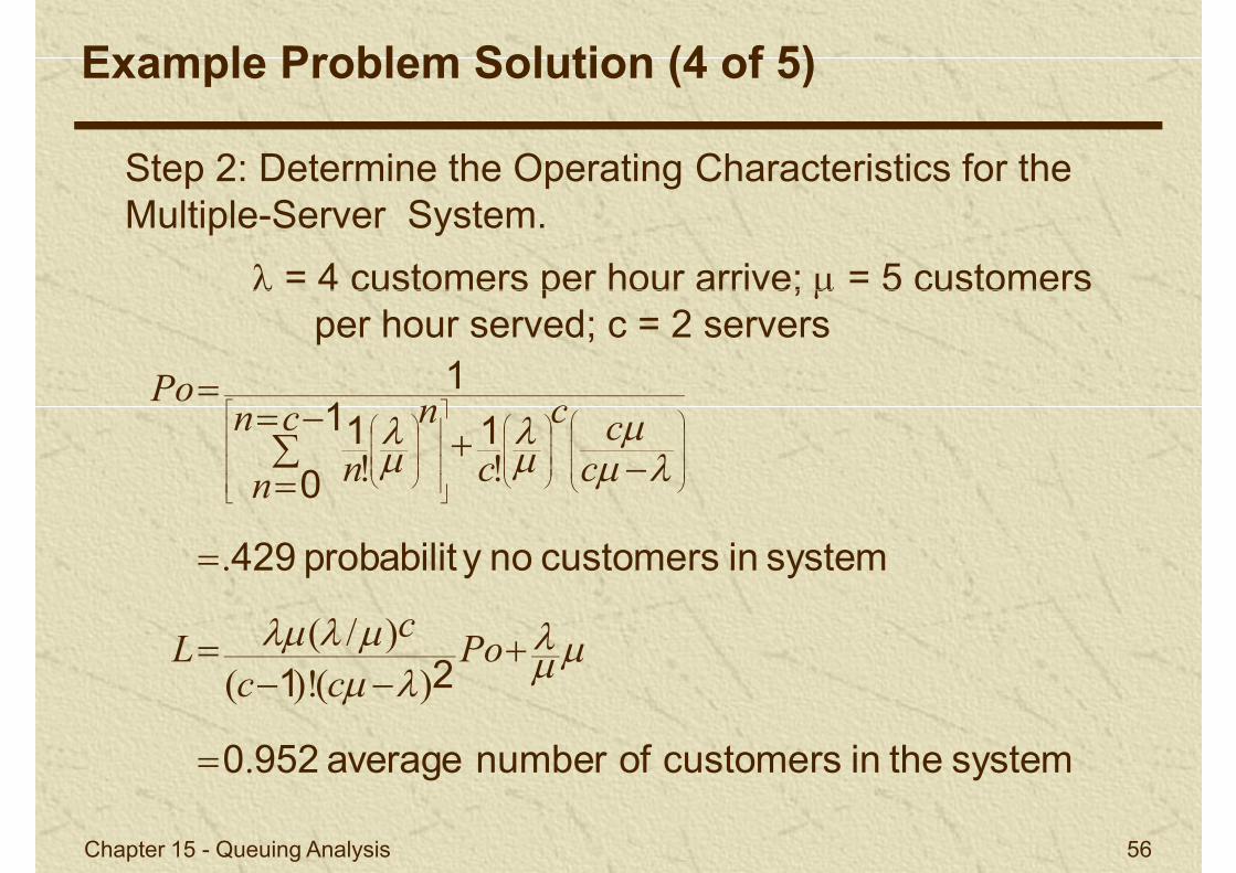
Step 2: Determine the Operating Characteristics for the Multiple-Server System.
= 4 customers per hour arrive; = 5 customers
Example Problem Solution (4 of 5)
systemincustomersnoy probabilit429
11
01
1
.
!!
ccc
ccn
n
n
n
Po
= 4 customers per hour arrive; = 5 customers per hour served; c = 2 servers
Chapter 15 - Queuing Analysis 56
systemtheincustomersofnumberaverage9520
21
.
)()!()/(
Po
cc
cL
LLq
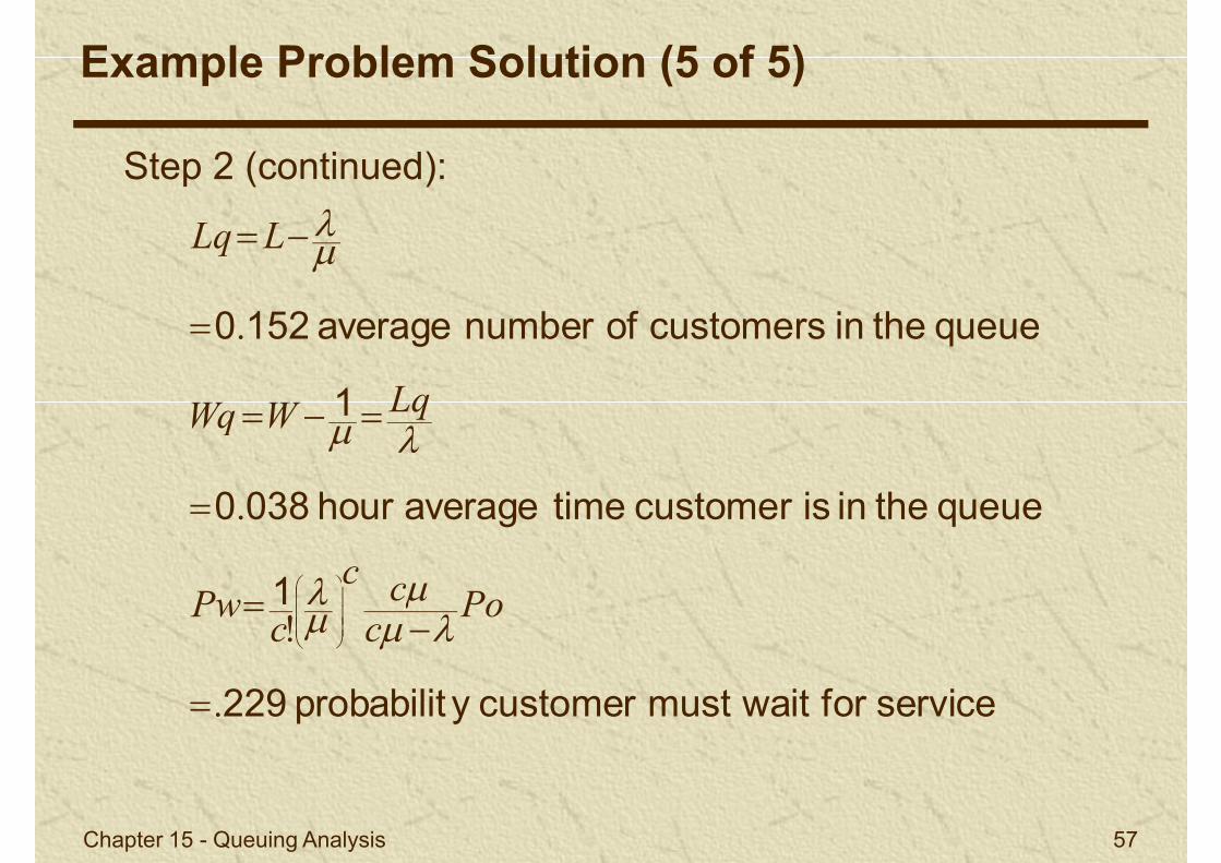
Step 2 (continued):
Example Problem Solution (5 of 5)
1
queuetheiniscustomertimeaveragehour0380
1
queuetheincustomersofnumberaverage1520
.
.
cc
LqWWq
Chapter 15 - Queuing Analysis 57
servicefor waitmustcustomery probabilit229
1
.
!
Po
ccc
cPw
Chapter 15 - Queuing Analysis 58


