149
Queuing Theory and Traffic Analysis CS 552 Richard Martin Rutgers University
Queuing Theoryand Traffic Analysis
CS 552Richard Martin
Rutgers University
Queuing theory
• View network as collections of queues– FIFO data-structures
• Queuing theory provides probabilisticanalysis of these queues
• Examples:– Average length– Probability queue is at a certain length– Probability a packet will be lost
Little’s Law
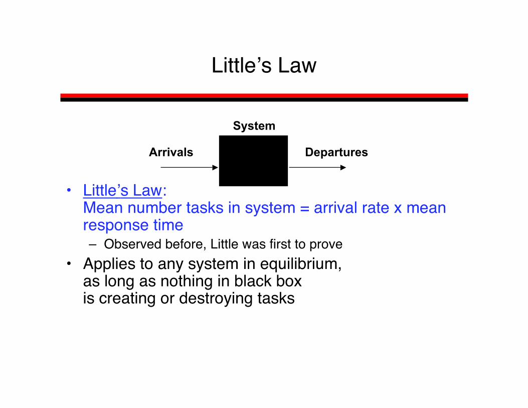
• Little’s Law:Mean number tasks in system = arrival rate x meanresponse time– Observed before, Little was first to prove
• Applies to any system in equilibrium,as long as nothing in black boxis creating or destroying tasks
Arrivals Departures
System
Proving Little’s Law
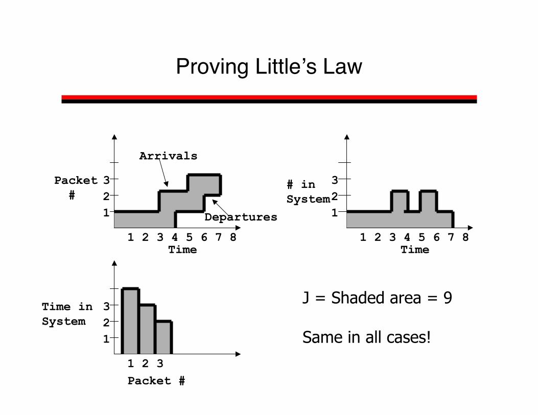
J = Shaded area = 9
Same in all cases!
1 2 3 4 5 6 7 8
Packet #
Time
123
1 2 3 4 5 6 7 8
# in System
123
Time
1 2 3
Time inSystem
Packet #
123
Arrivals
Departures
Definitions
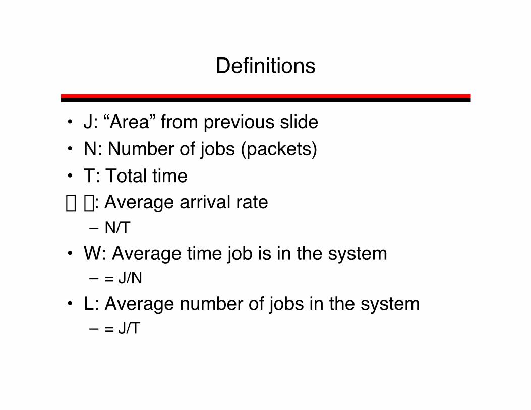
• J: “Area” from previous slide• N: Number of jobs (packets)• T: Total time" l: Average arrival rate
– N/T• W: Average time job is in the system
– = J/N• L: Average number of jobs in the system
– = J/T
1 2 3 4 5 6 7 8
# in System(L) 1
23
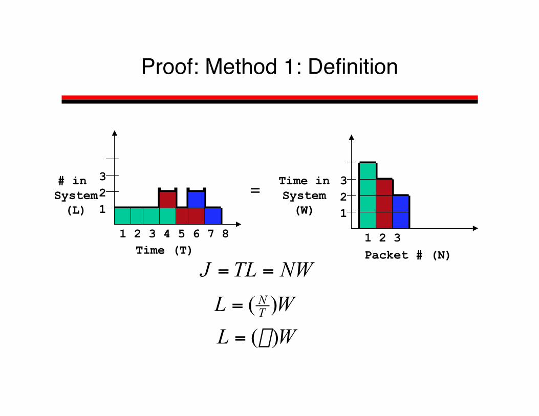
Proof: Method 1: Definition
Time (T) 1 2 3
Time inSystem(W)
Packet # (N)
123
=
WL TN )(=
NWTLJ ==
WL )(l=
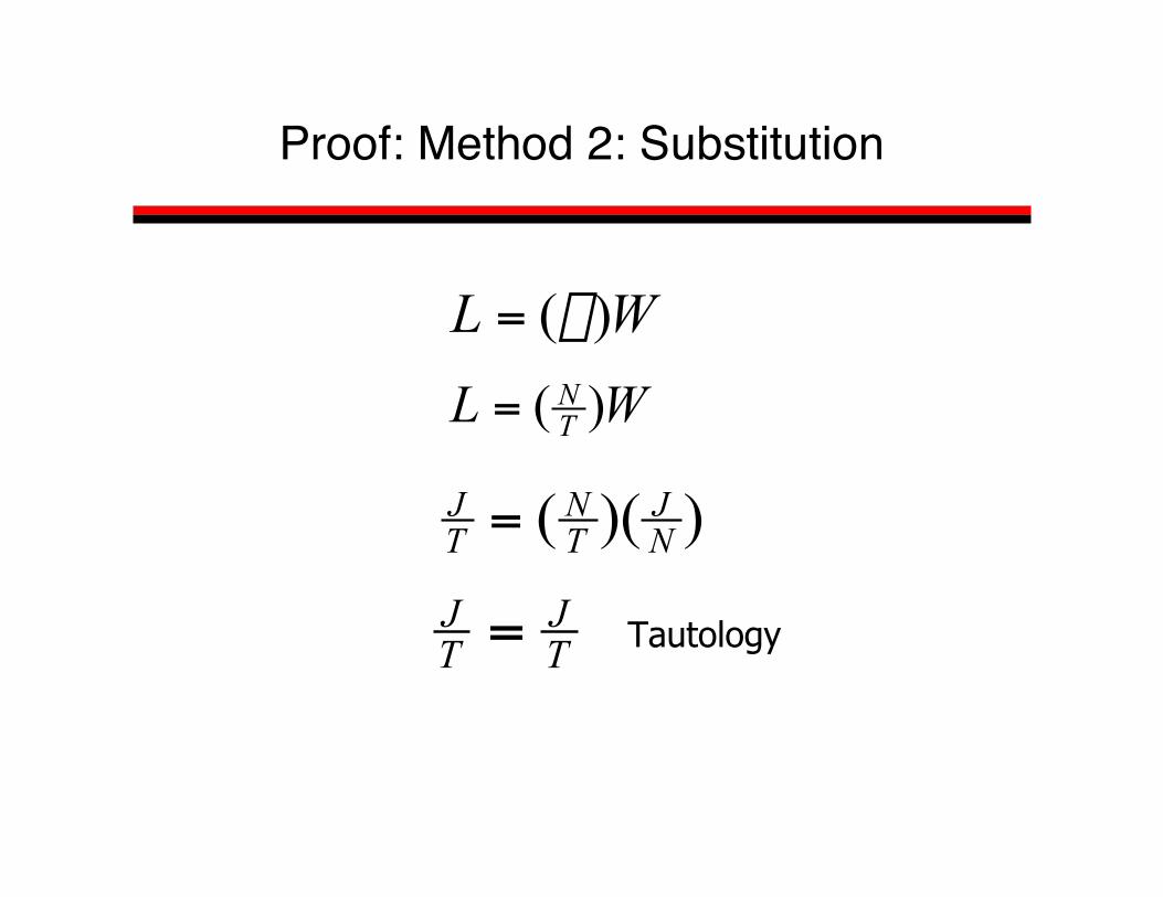
Proof: Method 2: Substitution
WL TN )(=
WL )(l=
))(( NJ
TN
TJ =
TJ
TJ = Tautology
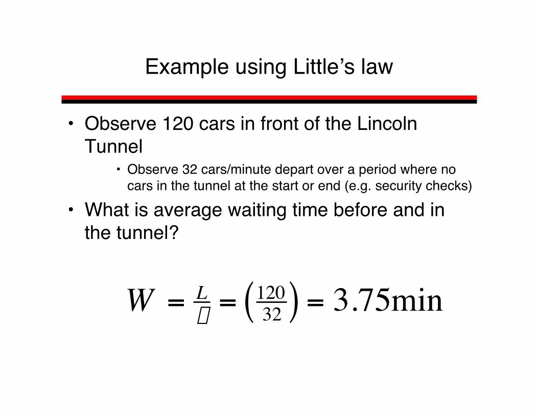
Example using Little’s law
• Observe 120 cars in front of the LincolnTunnel
• Observe 32 cars/minute depart over a period where nocars in the tunnel at the start or end (e.g. security checks)
• What is average waiting time before and inthe tunnel?
†
W = Ll = 120
32( ) = 3.75min

Model Queuing System
Strategy:Use Little’s law on both the complete system and its
parts to reason about average time in the queue
Server System Queuing System
Queue Server
Queuing System
lm
l

Kendal Notation
• Six parameters in shorthand• First three typically used, unless specified
1. Arrival Distribution• Probability of a new packet arrives in time t
2. Service Distribution• Probability distribution packet is serviced in time t
3. Number of servers4. Total Capacity (infinite if not specified)5. Population Size (infinite)6. Service Discipline (FCFS/FIFO)

Distributions
• M: Exponential• D: Deterministic (e.g. fixed constant)• Ek: Erlang with parameter k• Hk: Hyperexponential with param. k• G: General (anything)
• M/M/1 is the simplest ‘realistic’ queue
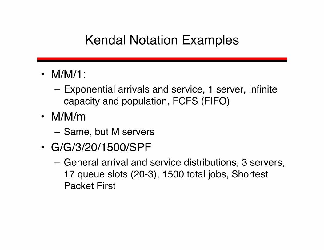
Kendal Notation Examples
• M/M/1:– Exponential arrivals and service, 1 server, infinite
capacity and population, FCFS (FIFO)• M/M/m
– Same, but M servers• G/G/3/20/1500/SPF
– General arrival and service distributions, 3 servers,17 queue slots (20-3), 1500 total jobs, ShortestPacket First
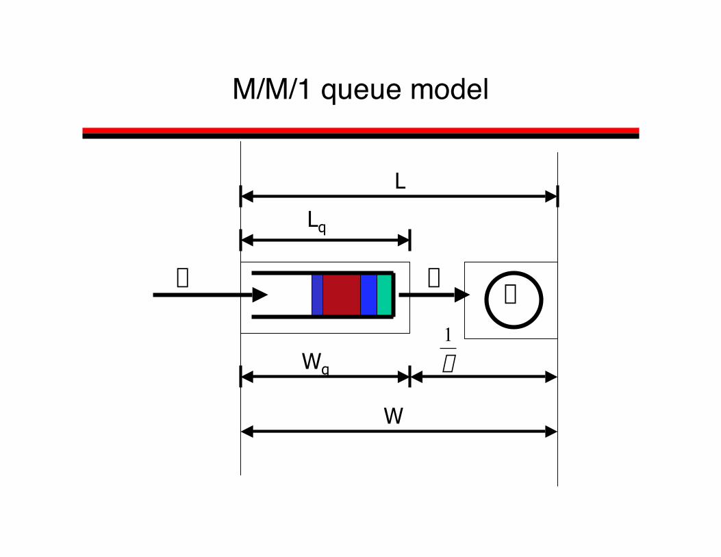
M/M/1 queue model
lm
l
m1
Wq
W
L
Lq

Analysis of M/M/1 queue
• Goal: A closed form expression of theprobability of the number of jobs in the queue(Pi) given only l and m
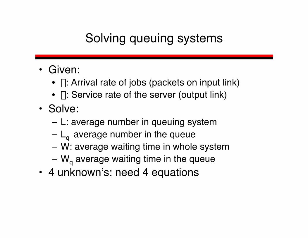
Solving queuing systems
• Given:• l: Arrival rate of jobs (packets on input link)• m: Service rate of the server (output link)
• Solve:– L: average number in queuing system– Lq average number in the queue– W: average waiting time in whole system– Wq average waiting time in the queue
• 4 unknown’s: need 4 equations
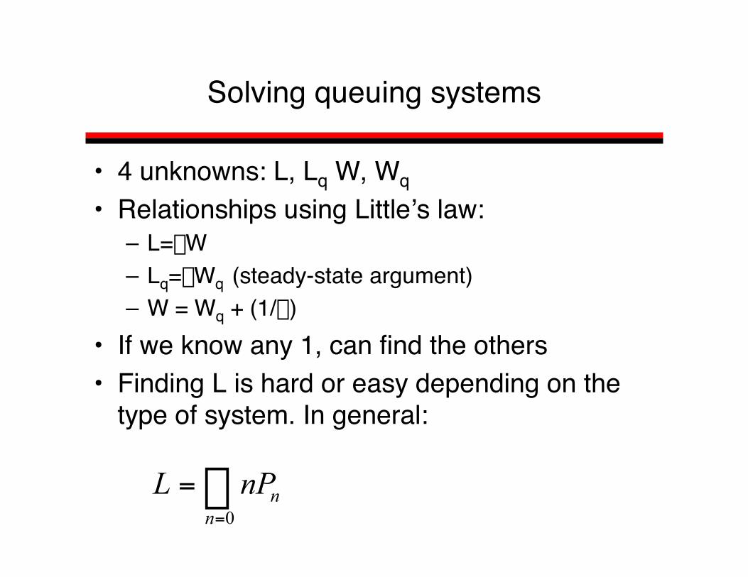
Solving queuing systems
• 4 unknowns: L, Lq W, Wq• Relationships using Little’s law:
– L=lW– Lq=lWq (steady-state argument)– W = Wq + (1/m)
• If we know any 1, can find the others• Finding L is hard or easy depending on the
type of system. In general:
0
•
=
=n
nnPL
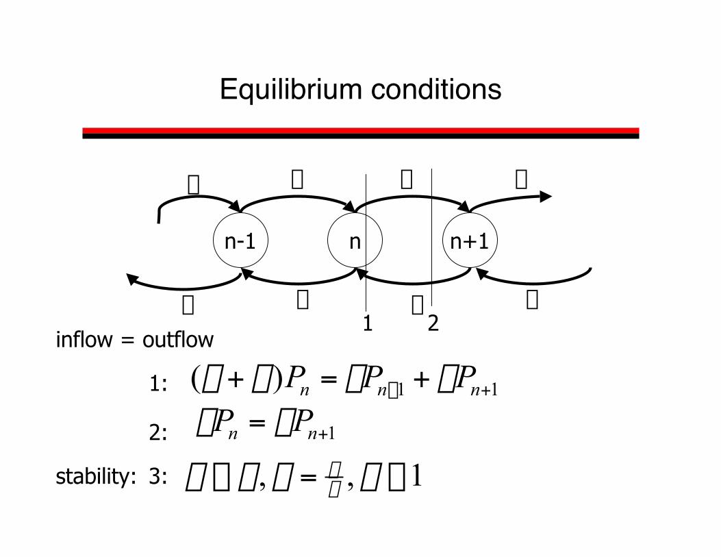
Equilibrium conditions
11)( +- +=+ nnn PPP mlml1:
2:
n+1nn-1
l l ll
m mm m
inflow = outflow 1 2
1+= nn PP ml
3:stability: 1,, £=£ rrml ml

Solving for P0 and Pn
01 PP r= ( ) 02
2 PP r= ( ) 0PP nn r=1:
•
=
=0
1n
nP •
=
=0
0 1n
nP rÂ
= •
=0
10
n
nP
r
2:
3: •
=
<-
=0
1,1
1
n
n rr
r (geometric series)
,
, ,
, ,
4:r
rr-==
Â=
-•
=
1)1(
1
0
110
n
nP 5: ( ) )1( rr -= n
nP

Solving for L
0
•
=
=n
nnPL )1(0
•
=
-=n
nn rr )1(1
1•
=
--=n
nnrrr
( )rrrr --= 11)1( d
d˜¯
ˆÁË
Ê- Â
=
1
0
)1(n
ndd rrr r
( )2)1(1)1(r
rr-
- lml
rr
-- == )1(

Solving W, Wq and Lq
( )( ) lmllml
l -- === 11LW
( ) ( ) )(11
lmml
mlml
m -- =-=-= WWq
)()(
2
lmml
lmmlll -- === qq WL
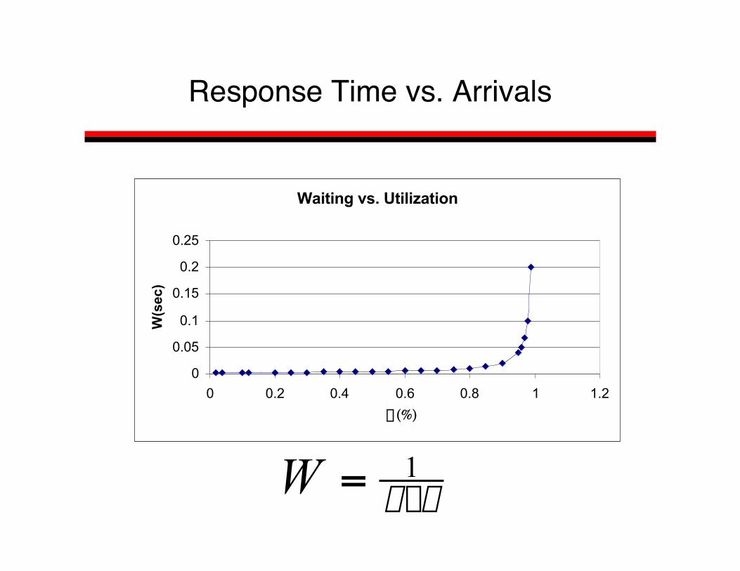
Response Time vs. Arrivals
lm-= 1W
Waiting vs. Utilization
0
0.05
0.1
0.15
0.2
0.25
0 0.2 0.4 0.6 0.8 1 1.2
r (%)
W(s
ec)

Stable Region
Waiting vs. Utilization
0
0.005
0.01
0.015
0.02
0.025
0 0.2 0.4 0.6 0.8 1
r (%)
W(s
ec)
linear region
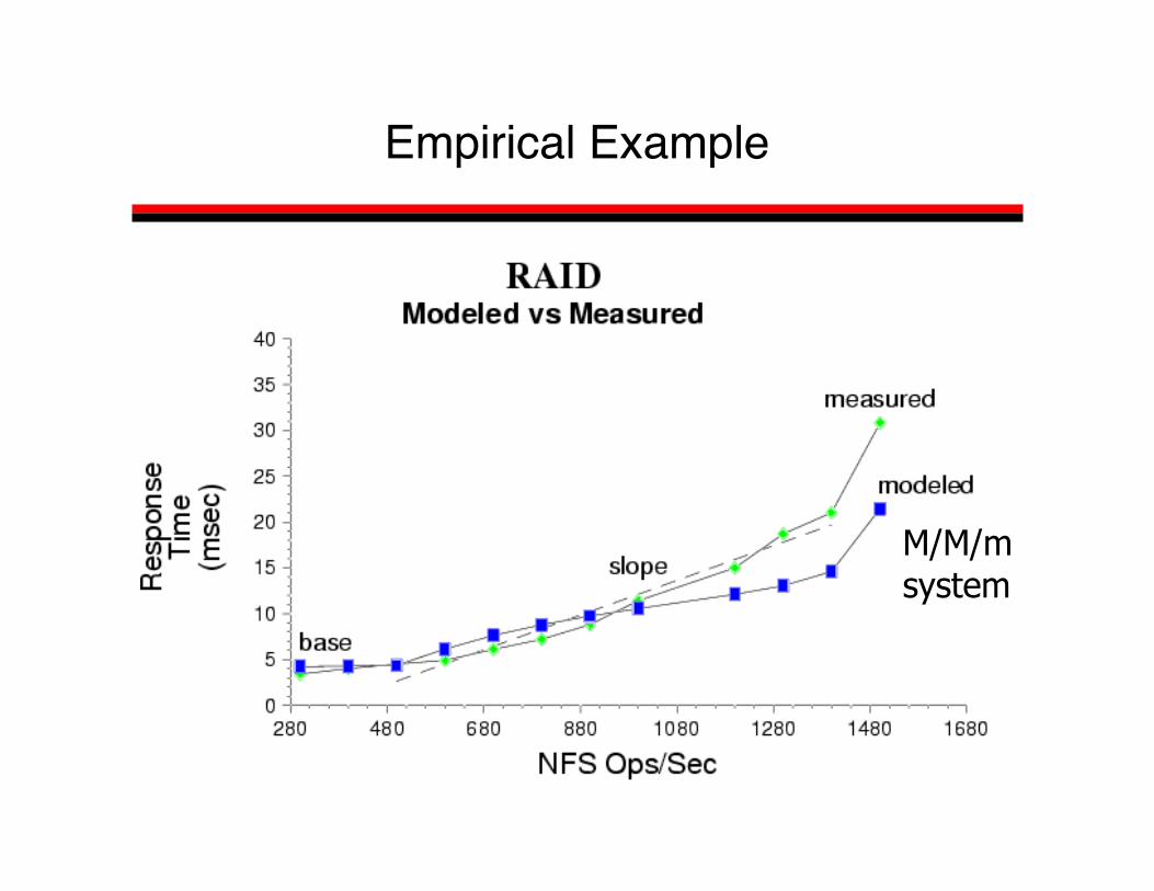
Empirical Example
M/M/msystem
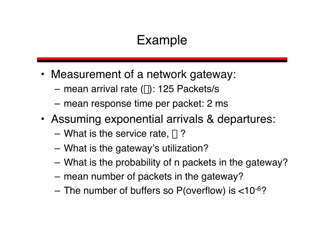
Example
• Measurement of a network gateway:– mean arrival rate (l): 125 Packets/s– mean response time per packet: 2 ms
• Assuming exponential arrivals & departures:– What is the service rate, m ?– What is the gateway’s utilization?– What is the probability of n packets in the gateway?– mean number of packets in the gateway?– The number of buffers so P(overflow) is <10-6?
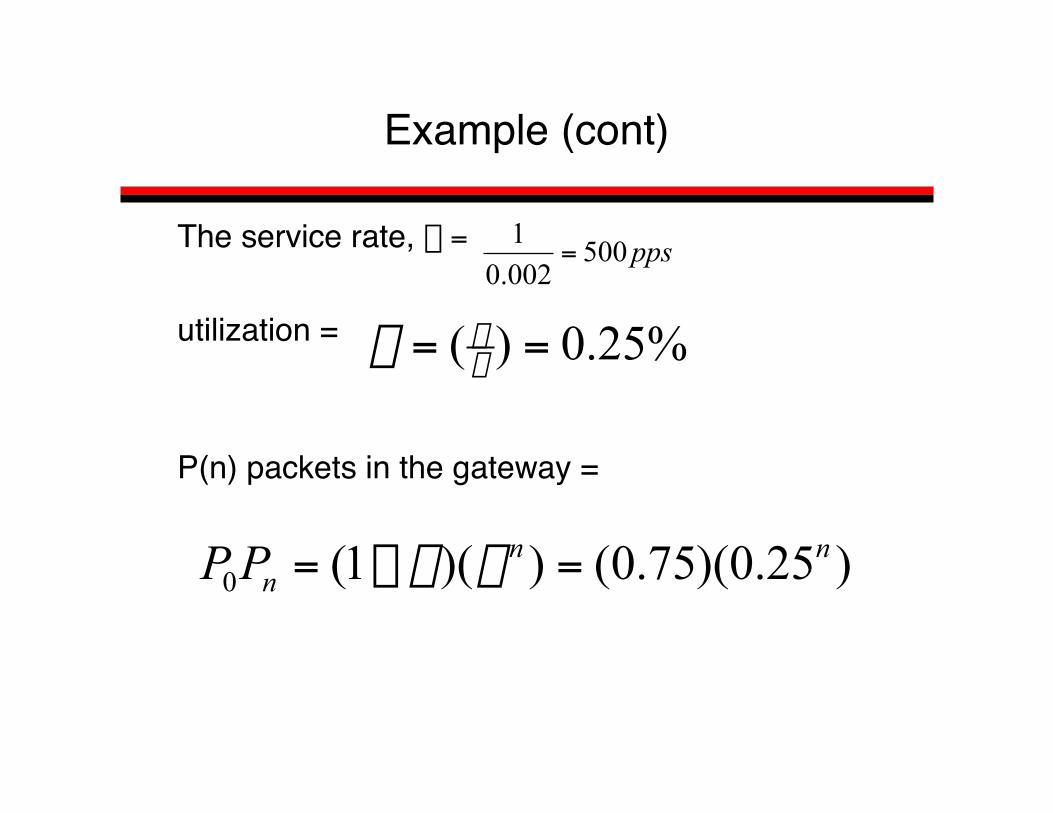
The service rate, m =
utilization =
P(n) packets in the gateway =
Example (cont)
pps500002.01
=
%25.0)( == mlr
)25.0)(75.0())(1(0nn
nPP =-= rr
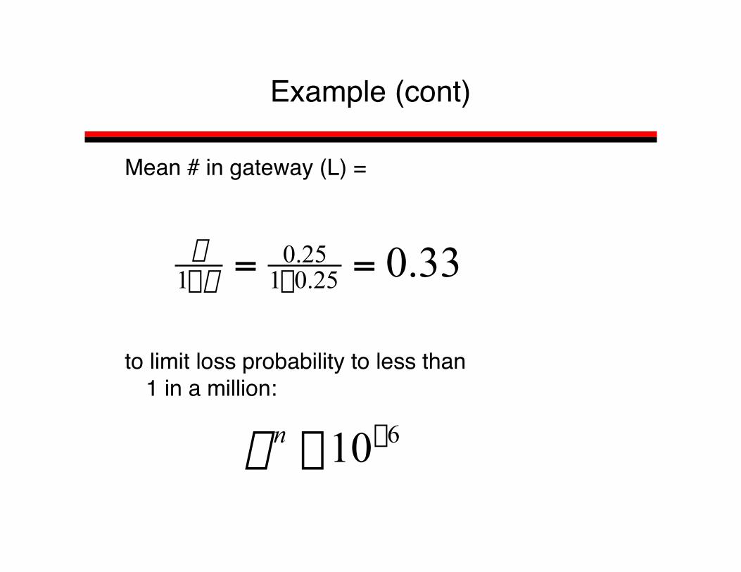
Mean # in gateway (L) =
to limit loss probability to less than1 in a million:
Example (cont)
33.025.0125.0
1 == --rr
610-£nr

• Poisson process = exponential distributionbetween arrivals/departures/service
• Key properties:– memoryless
– Past state does not help predict next arrival– Closed under:
– Addition– Subtraction
Properties of a Poisson processes
tetP l--=< 1)arrival(
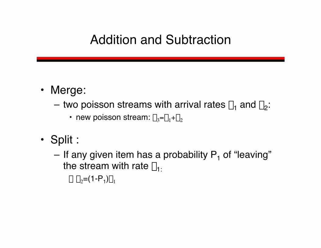
Addition and Subtraction
• Merge:– two poisson streams with arrival rates l1 and l2:
• new poisson stream: l3=l1+l2
• Split :– If any given item has a probability P1 of “leaving”
the stream with rate l1:" l2=(1-P1)l1

Queuing Networks
l1l2
l3 l4
l5
†
l1 = l2 + l3
†
l3 = l4 + l5
426 lll +=
l6
l7
57 ll =
0.3
0.5
0.7
0.5

Bridging Router Performance andQueuing Theory
Sigmetrics 2004
Slides by N. Hohn*, D. Veitch*, K.Papagiannaki, C. Diot
• End-to-end packet delay is an importantmetric for performance and Service LevelAgreements (SLAs)
• Building block of end-to-end delay is throughrouter delay
• Measure the delays incurred by all packetscrossing a single router
Motivation
Overview
• Full Router Monitoring• Delay Analysis and Modeling• Delay Performance: Understanding and
Reporting
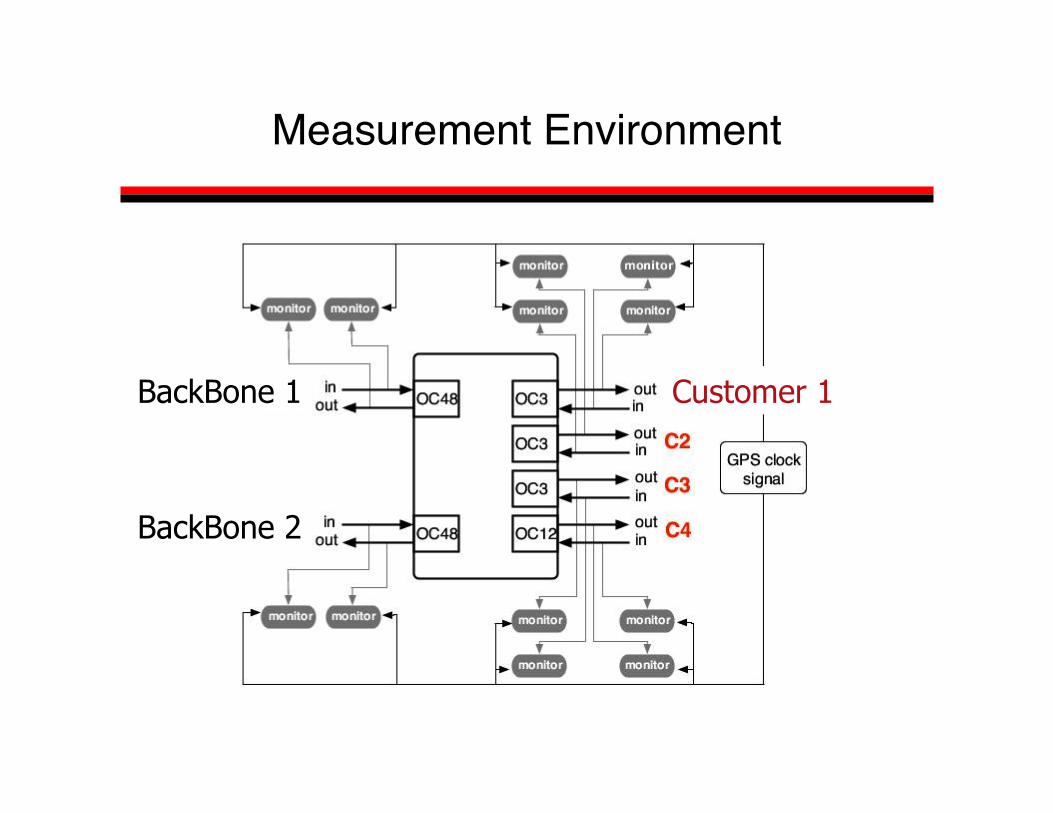
Measurement Environment
BackBone 1
BackBone 2
Customer 1
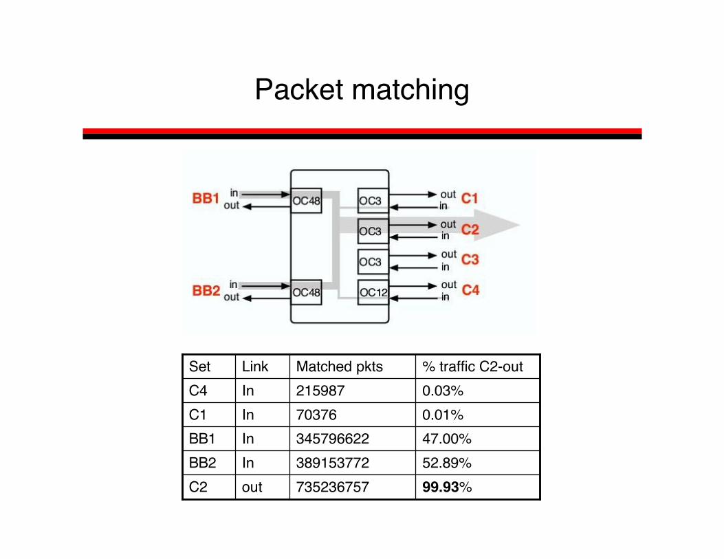
Packet matching
99.93%735236757outC252.89%389153772InBB247.00%345796622InBB10.01%70376InC10.03%215987InC4% traffic C2-outMatched pktsLinkSet

Overview
••• Full Router MonitoringFull Router MonitoringFull Router Monitoring• Delay Analysis and Modeling••• Delay Performance: Understanding andDelay Performance: Understanding andDelay Performance: Understanding and
ReportingReportingReporting

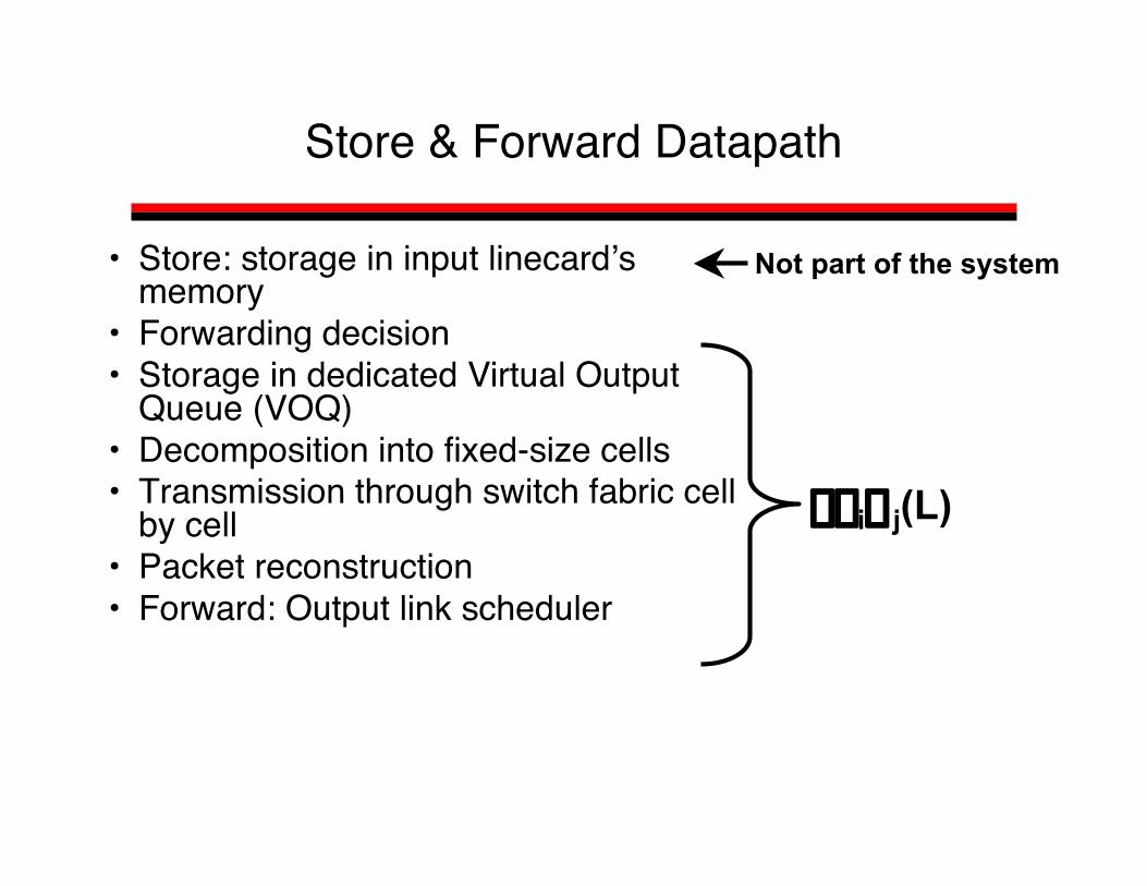
Definition of delay
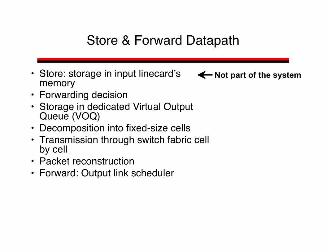
Store & Forward Datapath
• Store: storage in input linecard’smemory
• Forwarding decision• Storage in dedicated Virtual Output
Queue (VOQ)• Decomposition into fixed-size cells• Transmission through switch fabric cell
by cell• Packet reconstruction• Forward: Output link scheduler
Not part of the system

Delays: 1 minute summary
MAX
MIN
Mean
BB1-In to C2-Out
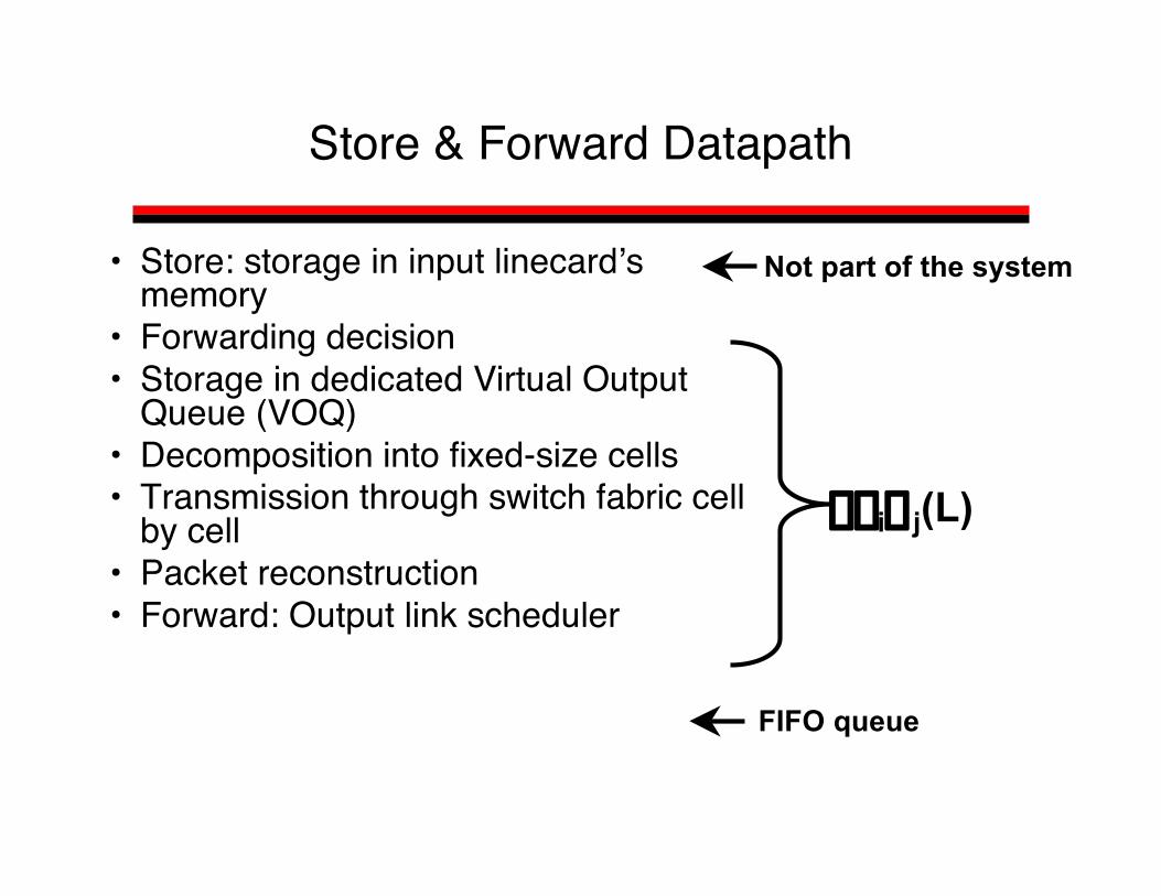
Store & Forward Datapath
• Store: storage in input linecard’smemory
• Forwarding decision• Storage in dedicated Virtual Output
Queue (VOQ)• Decomposition into fixed-size cells• Transmission through switch fabric cell
by cell• Packet reconstruction• Forward: Output link scheduler
Not part of the system
DliLj(L)
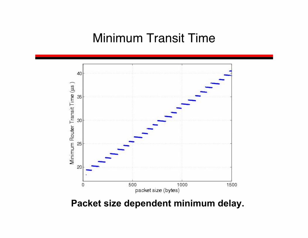
Minimum Transit Time
Packet size dependent minimum delay.
Store & Forward Datapath
• Store: storage in input linecard’smemory
• Forwarding decision• Storage in dedicated Virtual Output
Queue (VOQ)• Decomposition into fixed-size cells• Transmission through switch fabric cell
by cell• Packet reconstruction• Forward: Output link scheduler
Not part of the system
DliLj(L)
FIFO queue
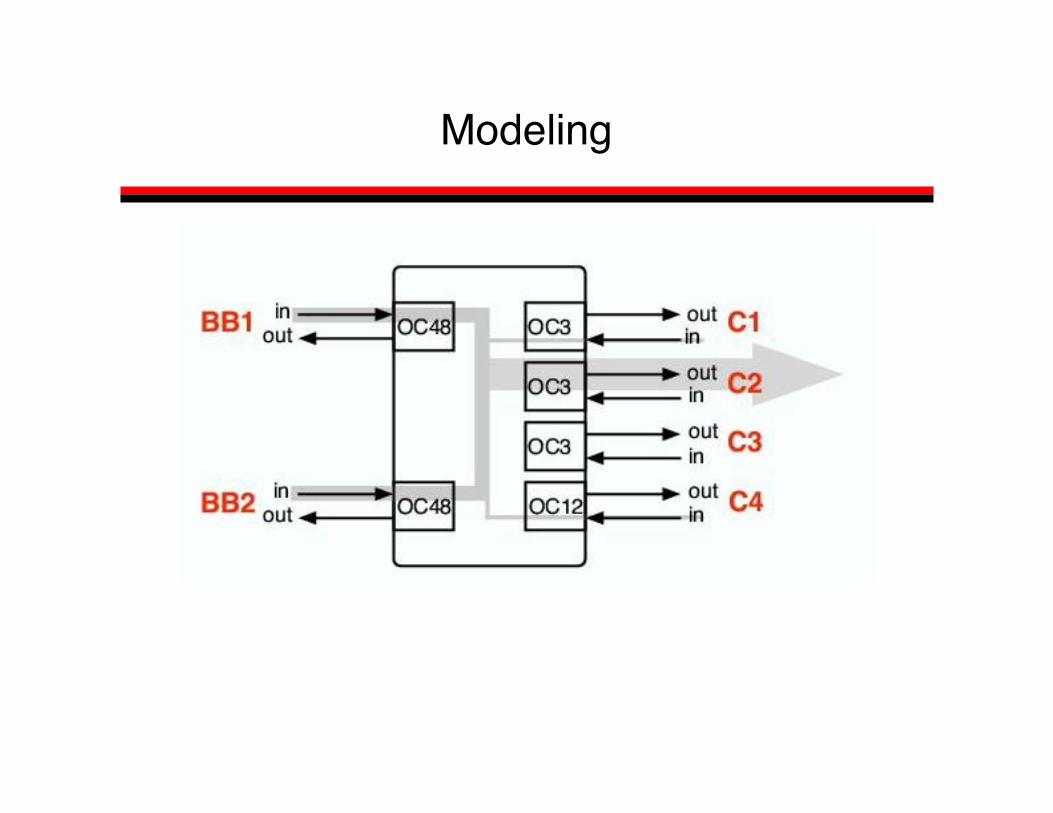
Modeling
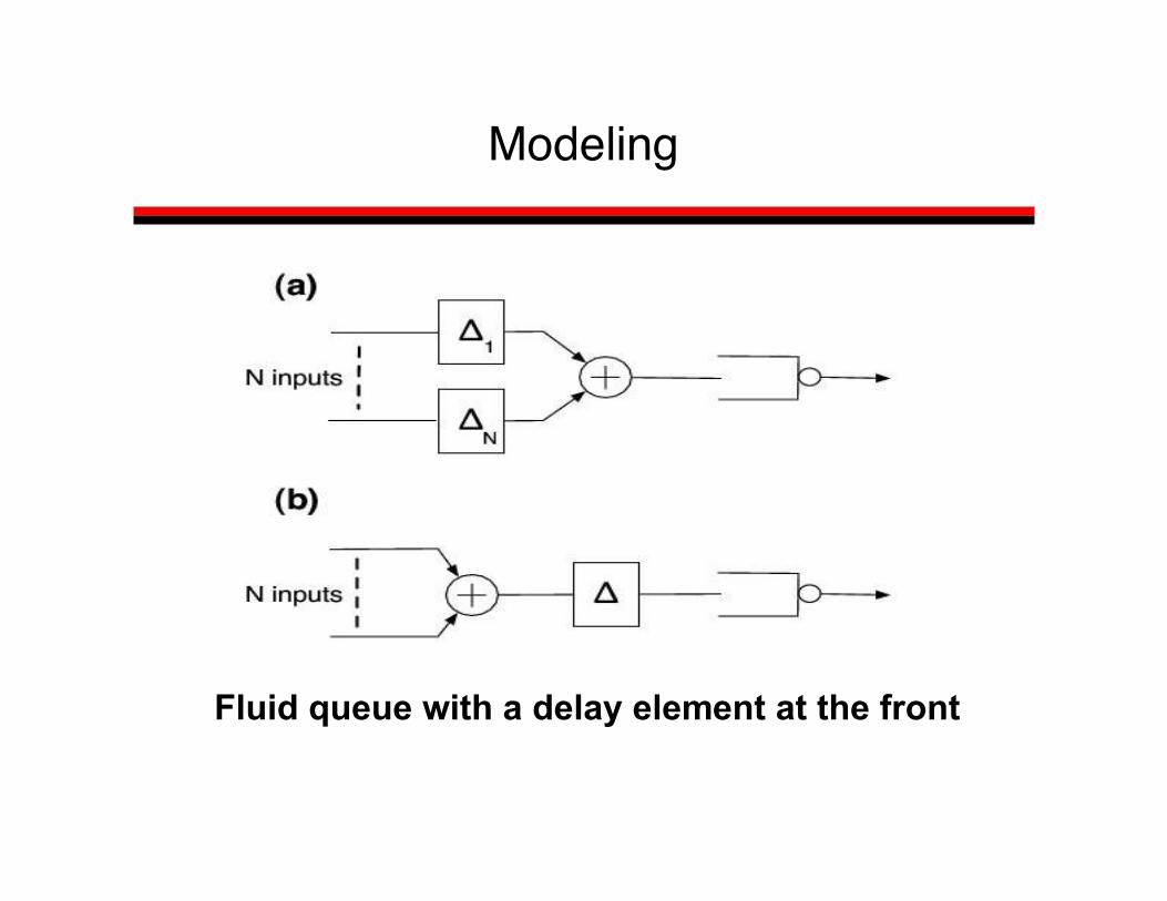
Modeling
Fluid queue with a delay element at the front

Model Validation
U(t)
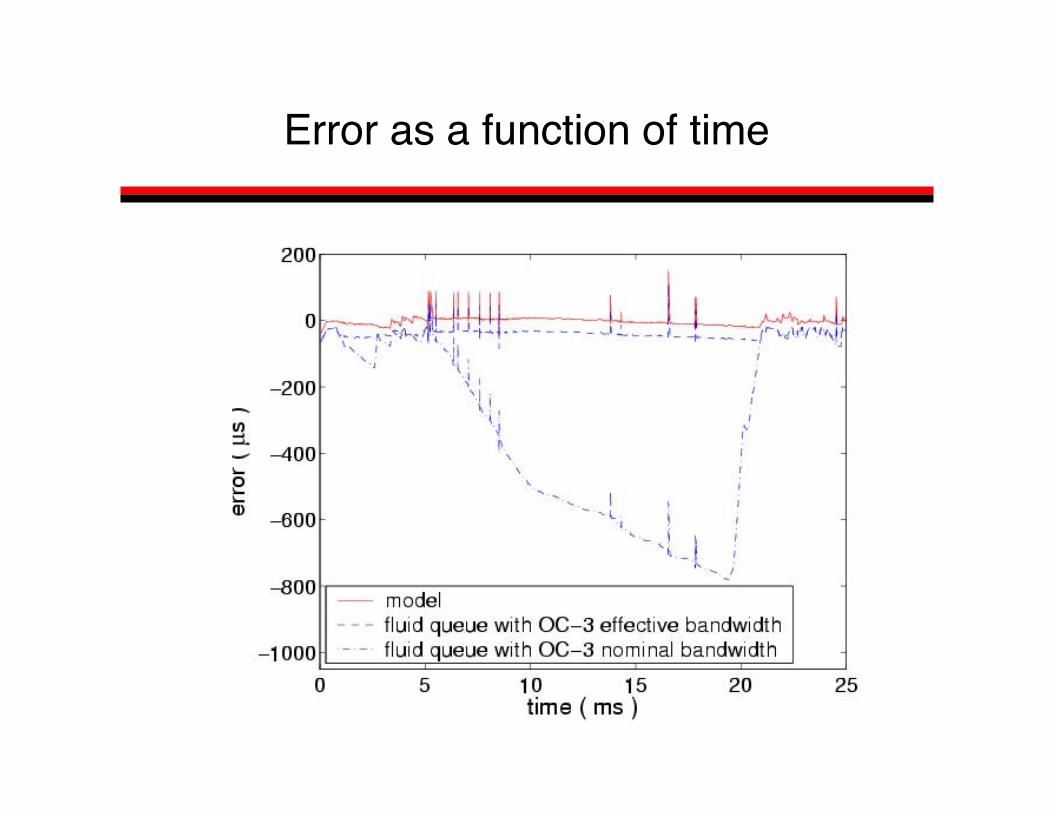
Error as a function of time
Modeling results
• A crude model performs well!– As simpler/simpler than an M/M/1 queue
• Use effective link bandwidth– account for encapsulation
• Small gap between router performance and queuingtheory!
• The model defines Busy Periods: time between thearrival of a packet to the empty system and the timewhen the system becomes empty again.
Overview
••• Full Router MonitoringFull Router MonitoringFull Router Monitoring••• Delay Analysis and ModelingDelay Analysis and ModelingDelay Analysis and Modeling• Delay Performance: Understanding and
Reporting
On the Delay Performance
• Model allows for router performanceevaluation when arrival patterns are known
• Goal: metrics that– Capture operational-router performance– Can answer performance questions directly
• Busy Period structures contain all delayinformation– BP better than utilization or delay reporting

Busy periods metrics
ts
D
A
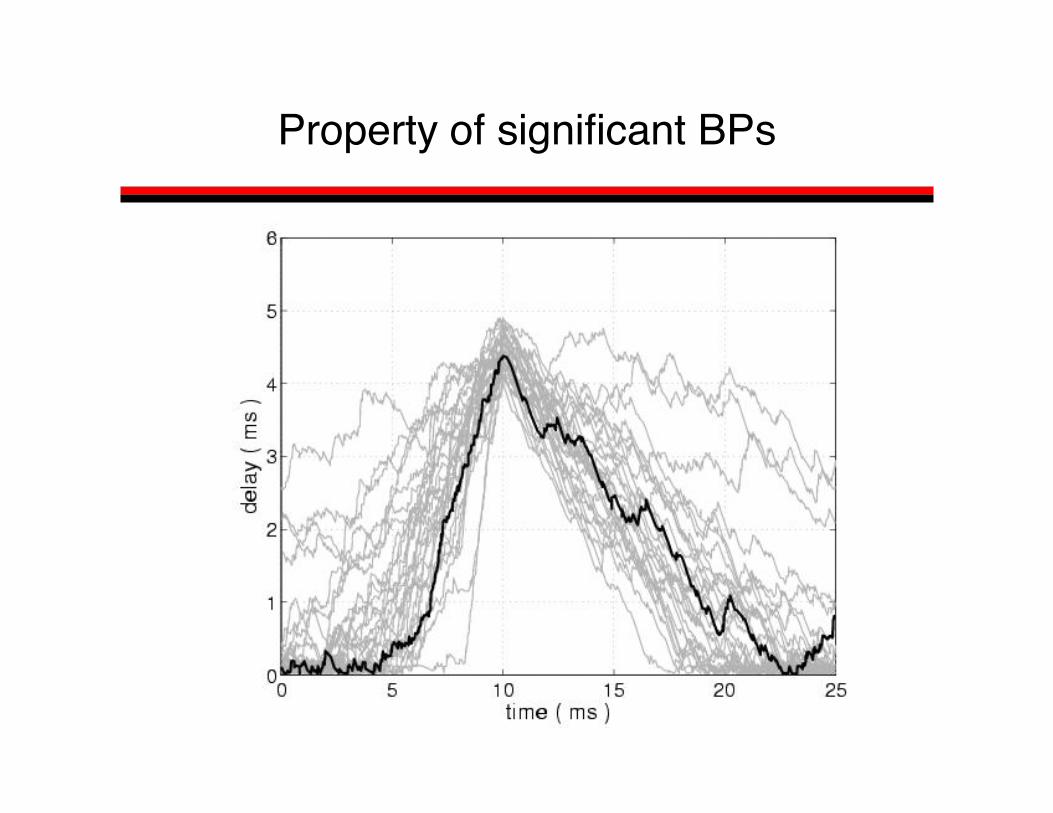
Property of significant BPs
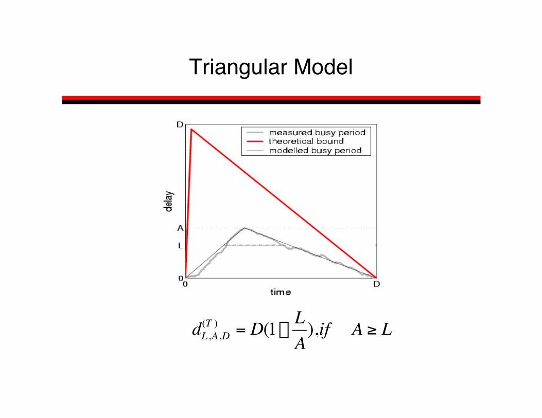
Triangular Model
†
dL ,A ,D(T ) = D(1-
LA
),if A ≥ L

Issues
• Report (A,D) measurements• There are millions of busy periods even on a
lightly utilized router• Interesting episodes are rare and last for a
very small amount of time
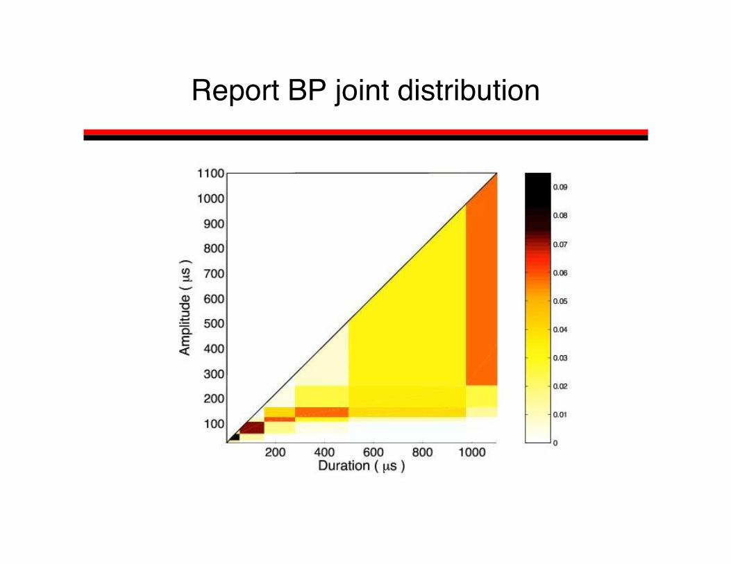
Report BP joint distribution
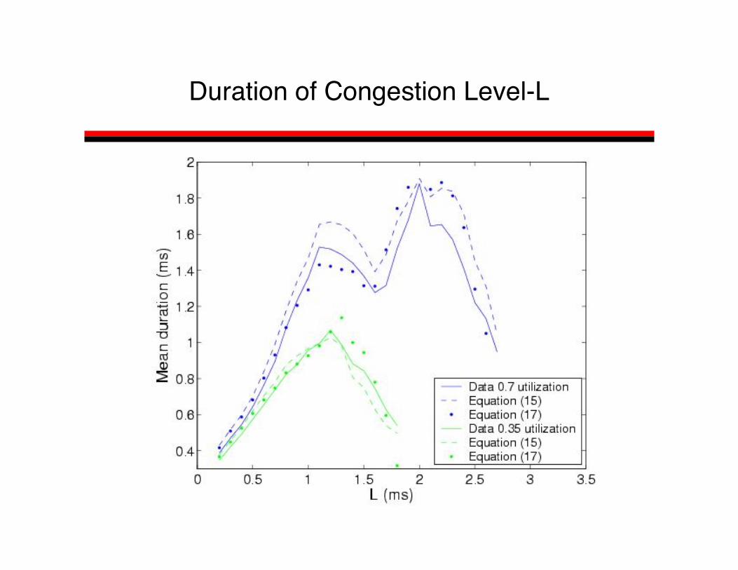
Duration of Congestion Level-L
Conclusions
• Results– Full router empirical study– Delay modeling– Reporting performance metrics
• Future work– Fine tune reporting scheme– Empirical evidence of large deviations theory

Network Traffic Self-SimilarityNetwork Traffic Self-Similarity
Slides by Carey WilliamsonDepartment of Computer Science
University of Saskatchewan
IntroductionIntroduction
• A classic measurement study has shown thataggregate Ethernet LAN traffic is self-similar[Leland et al 1993]
• A statistical property that is very different fromthe traditional Poisson-based models
• This presentation: definition of network trafficself-similarity, Bellcore Ethernet LAN data,implications of self-similarity
Measurement MethodologyMeasurement Methodology
• Collected lengthy traces of Ethernet LANtraffic on Ethernet LAN(s) at Bellcore
• High resolution time stamps• Analyzed statistical properties of the resulting
time series data• Each observation represents the number of
packets (or bytes) observed per time interval(e.g., 10 4 8 12 7 2 0 5 17 9 8 8 2...)

• If you plot the number of packets observedper time interval as a function of time, thenthe plot looks ‘‘the same’’ regardless of whatinterval size you choose
• E.g., 10 msec, 100 msec, 1 sec, 10 sec,...• Same applies if you plot number of bytes
observed per interval of time
Self-Similarity: The intuition

• In other words, self-similarity implies a‘‘fractal-like’’ behavior: no matter what timescale you use to examine the data, you seesimilar patterns
• Implications:– Burstiness exists across many time scales– No natural length of a burst– Key: Traffic does not necessarily get ‘‘smoother”
when you aggregate it (unlike Poisson traffic)
Self-Similarity: The Intuition
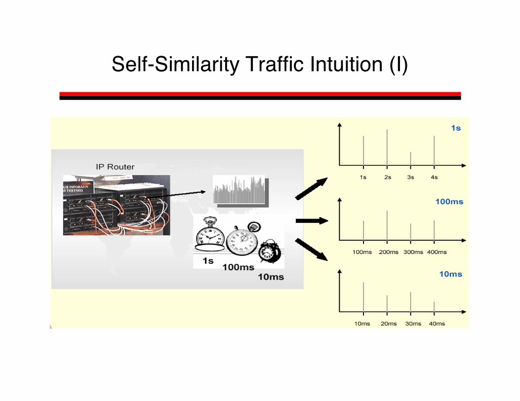
Self-Similarity Traffic Intuition (I)

Self-Similarity in Traffic Measurement II

• Self-similarity is a rigorous statistical property– (i.e., a lot more to it than just the pretty ‘‘fractal-
like’’ pictures)• Assumes you have time series data with finite
mean and variance– i.e., covariance stationary stochastic process
• Must be a very long time series– infinite is best!
• Can test for presence of self-similarity
Self-Similarity: The Math
• Self-similarity manifests itself in severalequivalent fashions:
• Slowly decaying variance• Long range dependence• Non-degenerate autocorrelations• Hurst effect
Self-Similarity: The Math
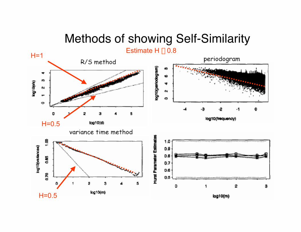
Methods of showing Self-Similarity
H=0.5
H=0.5
H=1Estimate H ª 0.8

• The variance of the sample decreases moreslowly than the reciprocal of the sample size
• For most processes, the variance of a samplediminishes quite rapidly as the sample size isincreased, and stabilizes soon
• For self-similar processes, the variancedecreases very slowly, even when the samplesize grows quite large
Slowly Decaying Variance
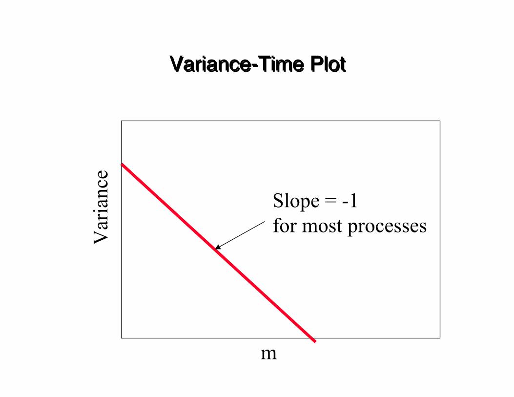
• The ‘‘variance-time plot” is one means to testfor the slowly decaying variance property
• Plots the variance of the sample versus thesample size, on a log-log plot
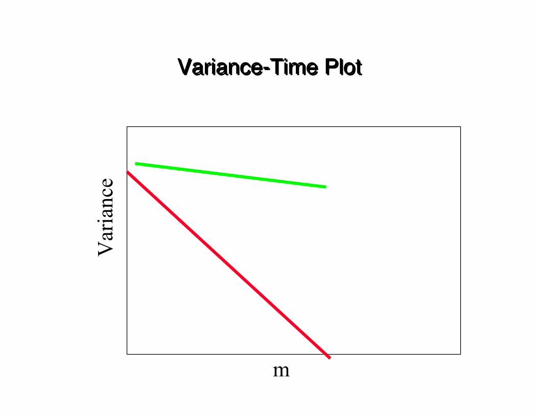
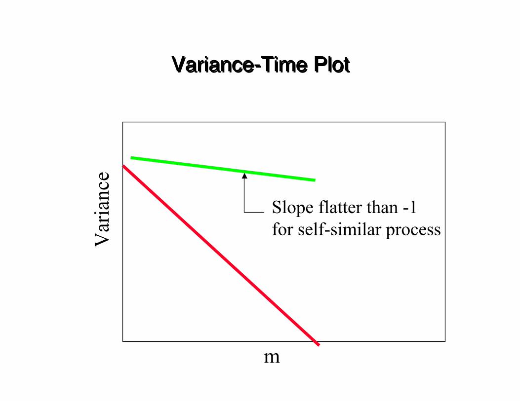
• For most processes, the result is a straightline with slope -1
• For self-similar, the line is much flatter
Time-Variance Plot
Var
ianc
e
m
Time Variance Plot

Variance-Time PlotVariance-Time PlotV
aria
nce
m
Variance of sampleon a logarithmic scale
0.0001
0.001
10.0
0.01
100.0
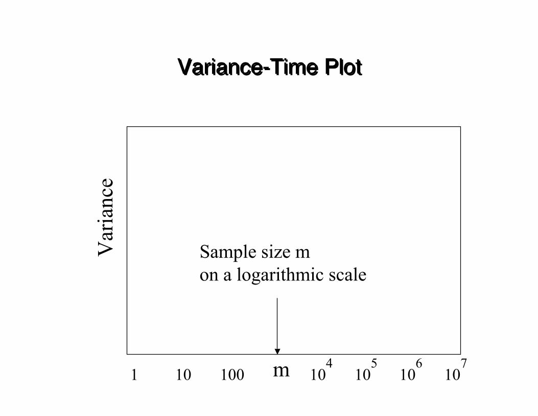
Variance-Time PlotVariance-Time PlotV
aria
nce
m
Sample size mon a logarithmic scale
1 10 100 10 10 10 104 5 6 7
Variance-Time PlotVariance-Time PlotV
aria
nce
m
Variance-Time PlotVariance-Time PlotV
aria
nce
m
Variance-Time PlotVariance-Time PlotV
aria
nce
m
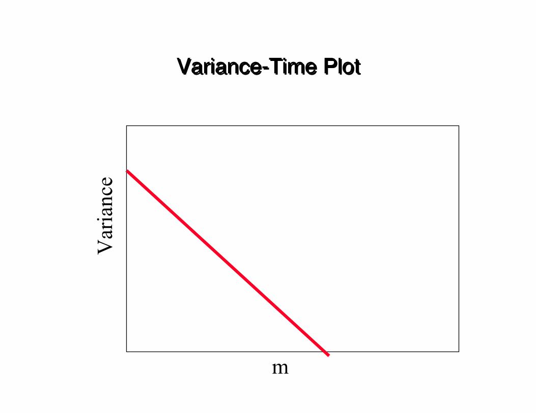
Slope = -1for most processes
Variance-Time PlotVariance-Time PlotV
aria
nce
m
Variance-Time PlotVariance-Time PlotV
aria
nce
m
Slope flatter than -1for self-similar process
• Correlation is a statistical measure of therelationship, if any, between two randomvariables
• Positive correlation: both behave similarly• Negative correlation: behave as opposites• No correlation: behavior of one is unrelated to
behavior of other
Long Range Dependence

• Autocorrelation is a statistical measure of therelationship, if any, between a randomvariable and itself, at different time lags
• Positive correlation: big observation usuallyfollowed by another big, or small by small
• Negative correlation: big observation usuallyfollowed by small, or small by big
• No correlation: observations unrelated
Long Range Dependence
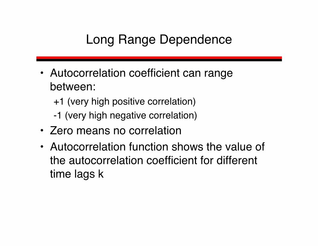
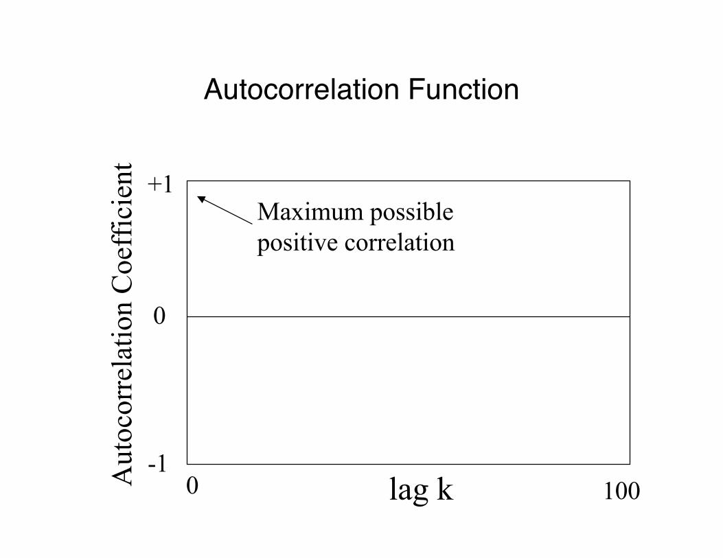
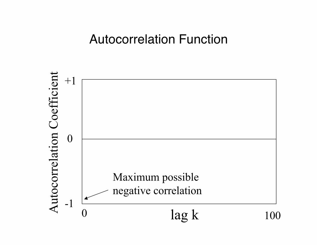
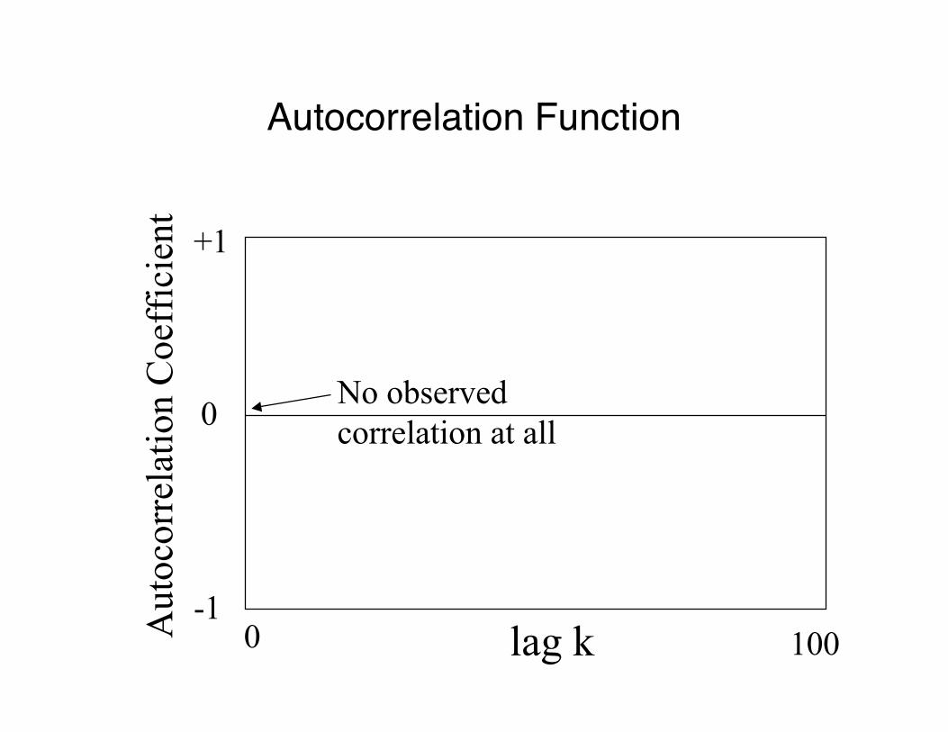
• Autocorrelation coefficient can rangebetween:+1 (very high positive correlation)-1 (very high negative correlation)
• Zero means no correlation• Autocorrelation function shows the value of
the autocorrelation coefficient for differenttime lags k
Long Range Dependence

+1
-1
0
lag k0 100Aut
ocor
rela
tion
Coe
ffic
ient
Autocorrelation Function
+1
-1
0
lag k0 100Aut
ocor
rela
tion
Coe
ffic
ient
Maximum possible positive correlation
Autocorrelation Function
+1
-1
0
lag k0 100Aut
ocor
rela
tion
Coe
ffic
ient
Maximum possiblenegative correlation
Autocorrelation Function
+1
-1
0
lag k0 100Aut
ocor
rela
tion
Coe
ffic
ient
No observedcorrelation at all
Autocorrelation Function
+1
-1
0
lag k0 100Aut
ocor
rela
tion
Coe
ffic
ient
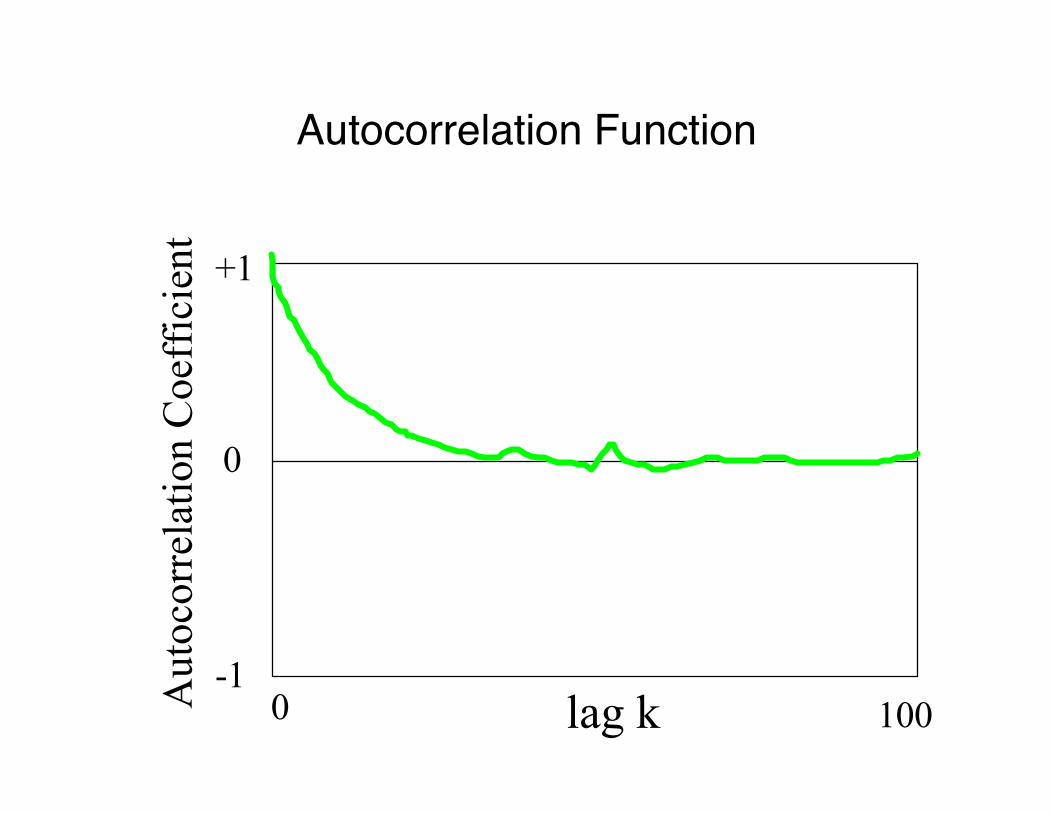
Autocorrelation Function
+1
-1
0
lag k0 100Aut
ocor
rela
tion
Coe
ffic
ient
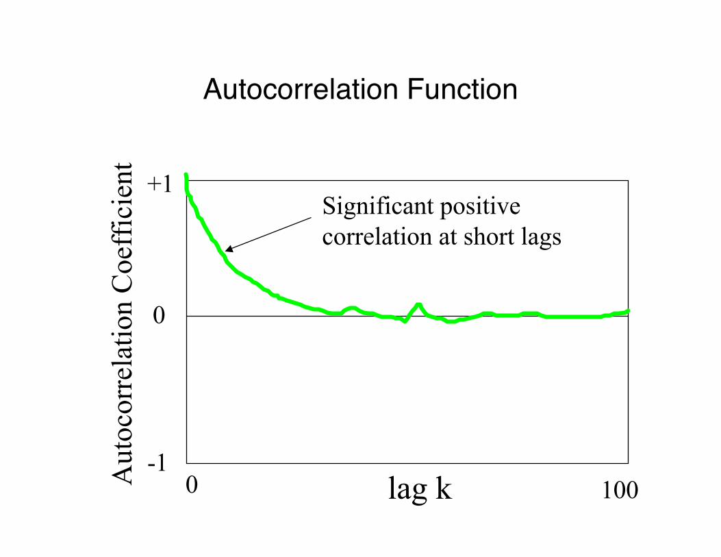
Significant positivecorrelation at short lags
Autocorrelation Function
+1
-1
0
lag k0 100Aut
ocor
rela
tion
Coe
ffic
ient
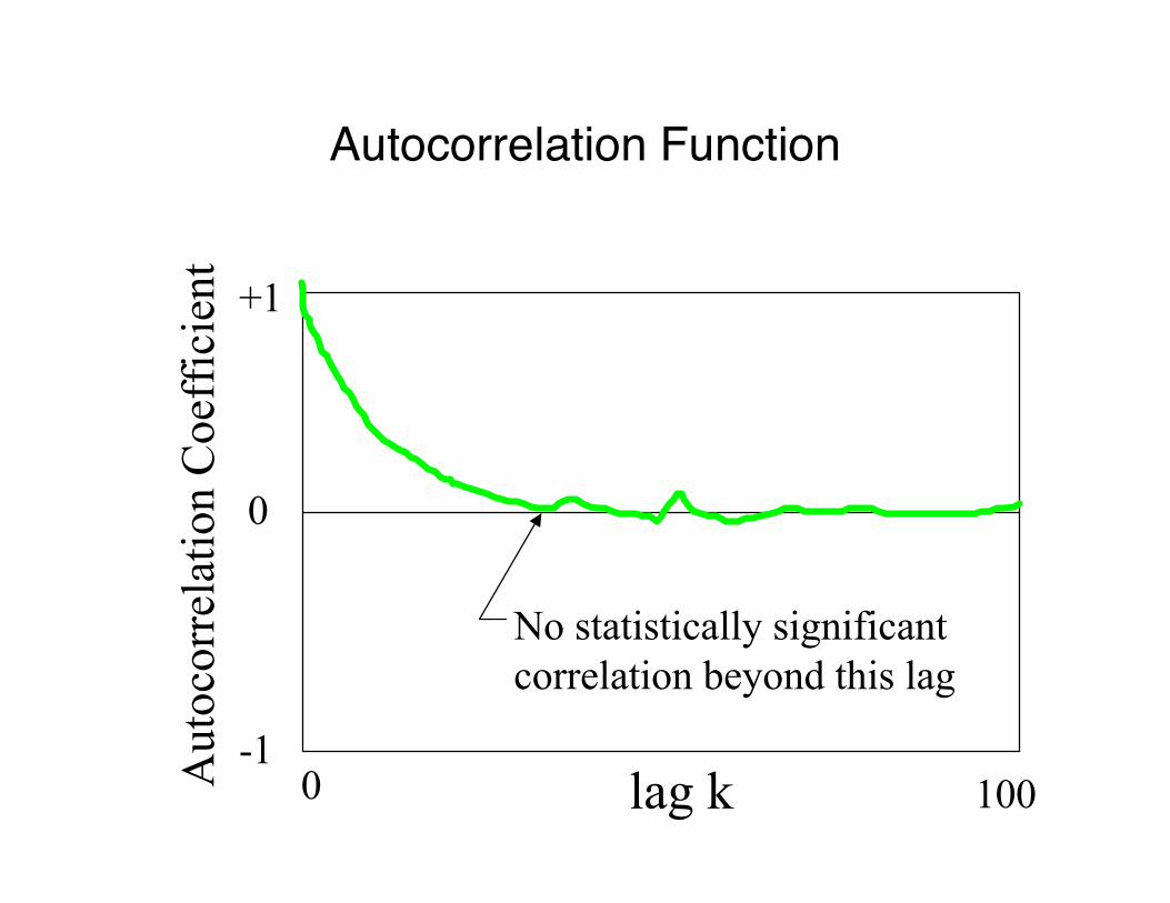
No statistically significantcorrelation beyond this lag
Autocorrelation Function

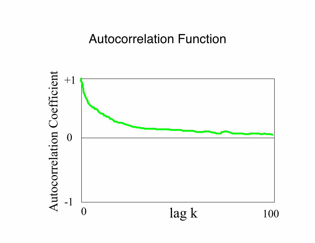
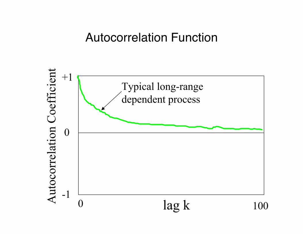
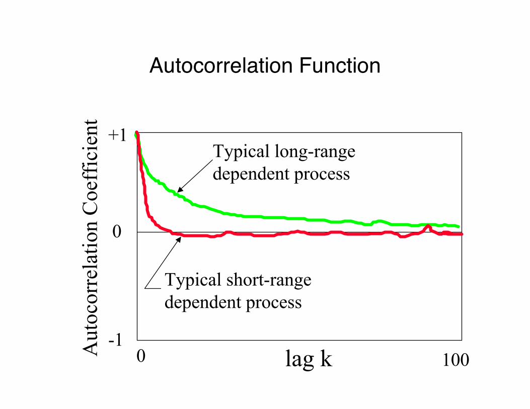
• For most processes (e.g., Poisson, orcompound Poisson), the autocorrelationfunction drops to zero very quickly– usually immediately, or exponentially fast
• For self-similar processes, the autocorrelationfunction drops very slowly– i.e., hyperbolically, toward zero, but may never
reach zero• Non-summable autocorrelation function
Long Range Dependence
+1
-1
0
lag k0 100Aut
ocor
rela
tion
Coe
ffic
ient
Autocorrelation Function

+1
-1
0
lag k0 100Aut
ocor
rela
tion
Coe
ffic
ient
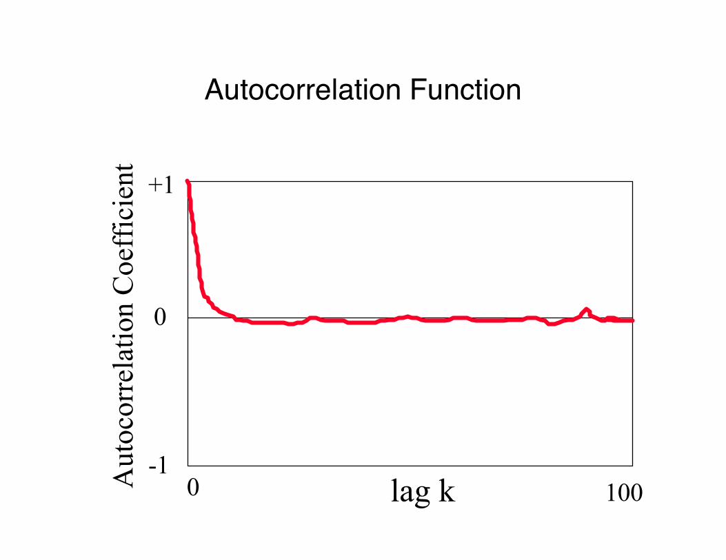
Typical short-rangedependent process
Autocorrelation Function
+1
-1
0
lag k0 100Aut
ocor
rela
tion
Coe
ffic
ient
Autocorrelation Function
+1
-1
0
lag k0 100Aut
ocor
rela
tion
Coe
ffic
ient
Typical long-range dependent process
Autocorrelation Function
+1
-1
0
lag k0 100Aut
ocor
rela
tion
Coe
ffic
ient
Typical long-range dependent process
Typical short-rangedependent process
Autocorrelation Function
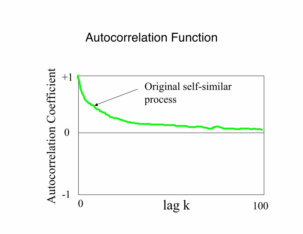
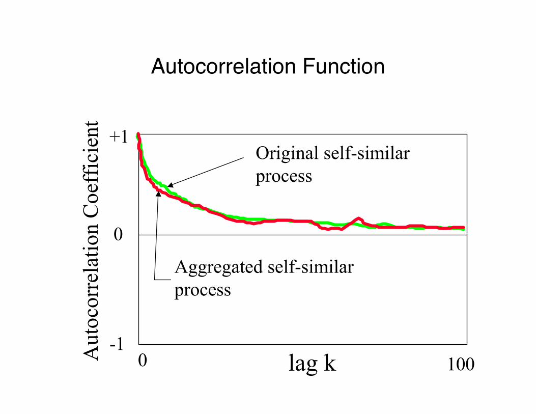
• For self-similar processes, the autocorrelationfunction for the aggregated process isindistinguishable from that of the originalprocess
• If autocorrelation coefficients match for alllags k, then called exactly self-similar
• If autocorrelation coefficients match only forlarge lags k, then called asymptotically self-similar
Non-Degenerate Autocorrelations
+1
-1
0
lag k0 100Aut
ocor
rela
tion
Coe
ffic
ient
Original self-similarprocess
Autocorrelation Function

+1
-1
0
lag k0 100Aut
ocor
rela
tion
Coe
ffic
ient
Original self-similarprocess
Autocorrelation Function
+1
-1
0
lag k0 100Aut
ocor
rela
tion
Coe
ffic
ient
Original self-similarprocess
Aggregated self-similarprocess
Autocorrelation Function
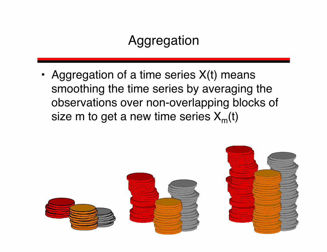
• Aggregation of a time series X(t) meanssmoothing the time series by averaging theobservations over non-overlapping blocks ofsize m to get a new time series Xm(t)
Aggregation
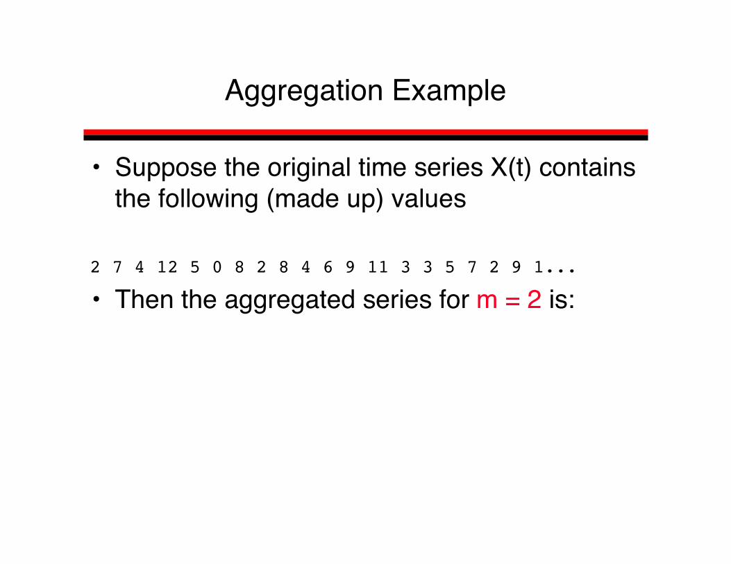
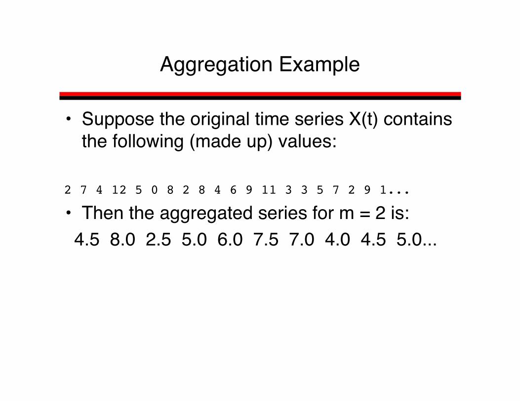
• Suppose the original time series X(t) containsthe following (made up) values
2 7 4 12 5 0 8 2 8 4 6 9 11 3 3 5 7 2 9 1...
• Then the aggregated series for m = 2 is:
Aggregation Example
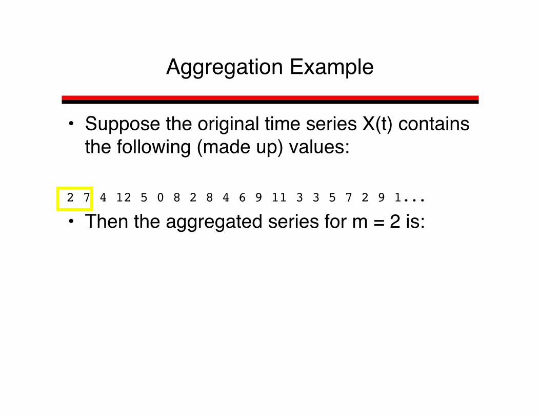
• Suppose the original time series X(t) containsthe following (made up) values:
2 7 4 12 5 0 8 2 8 4 6 9 11 3 3 5 7 2 9 1...
• Then the aggregated series for m = 2 is:
Aggregation Example
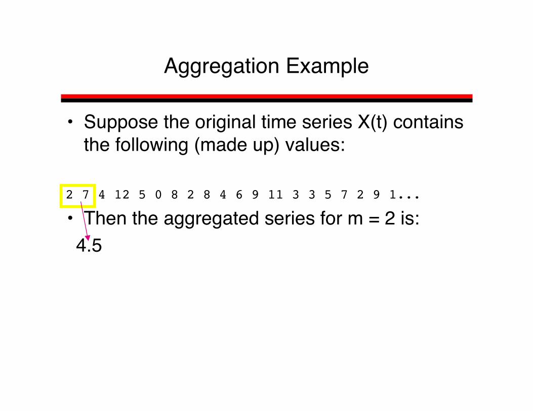
• Suppose the original time series X(t) containsthe following (made up) values:
2 7 4 12 5 0 8 2 8 4 6 9 11 3 3 5 7 2 9 1...
• Then the aggregated series for m = 2 is: 4.5
Aggregation Example

• Suppose the original time series X(t) containsthe following (made up) values:
2 7 4 12 5 0 8 2 8 4 6 9 11 3 3 5 7 2 9 1...
• Then the aggregated series for m = 2 is: 4.5 8.0
Aggregation example
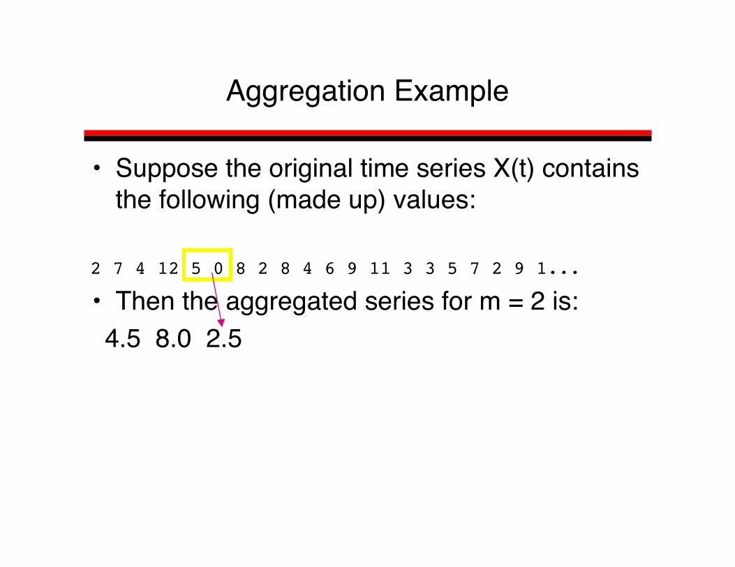
• Suppose the original time series X(t) containsthe following (made up) values:
2 7 4 12 5 0 8 2 8 4 6 9 11 3 3 5 7 2 9 1...
• Then the aggregated series for m = 2 is: 4.5 8.0 2.5
Aggregation Example
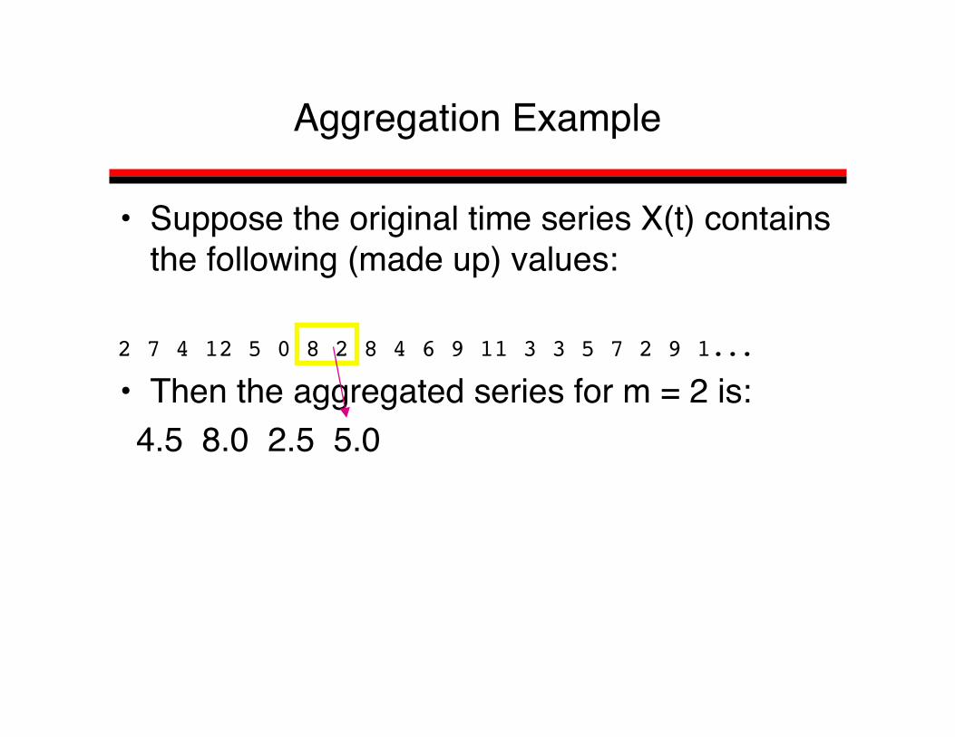
• Suppose the original time series X(t) containsthe following (made up) values:
2 7 4 12 5 0 8 2 8 4 6 9 11 3 3 5 7 2 9 1...
• Then the aggregated series for m = 2 is: 4.5 8.0 2.5 5.0
Aggregation Example
• Suppose the original time series X(t) containsthe following (made up) values:
2 7 4 12 5 0 8 2 8 4 6 9 11 3 3 5 7 2 9 1...
• Then the aggregated series for m = 2 is: 4.5 8.0 2.5 5.0 6.0 7.5 7.0 4.0 4.5 5.0...
Aggregation Example
• Suppose the original time series X(t) containsthe following (made up) values:
2 7 4 12 5 0 8 2 8 4 6 9 11 3 3 5 7 2 9 1...
Then the aggregated time series for m = 5 is:
Aggregation Example
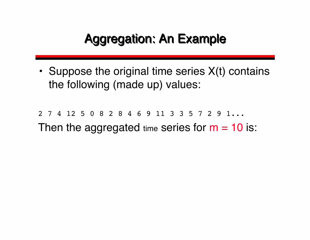
Aggregation: An ExampleAggregation: An Example
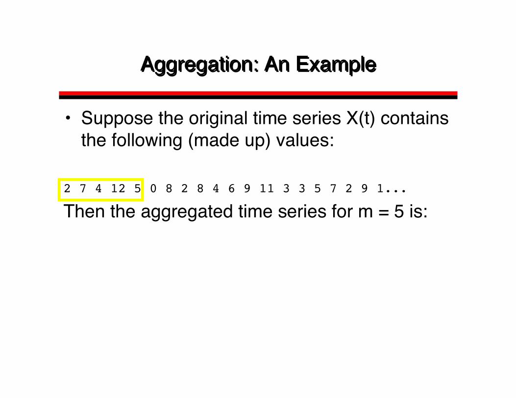
• Suppose the original time series X(t) containsthe following (made up) values:
2 7 4 12 5 0 8 2 8 4 6 9 11 3 3 5 7 2 9 1...
Then the aggregated time series for m = 5 is:
Aggregation: An ExampleAggregation: An Example
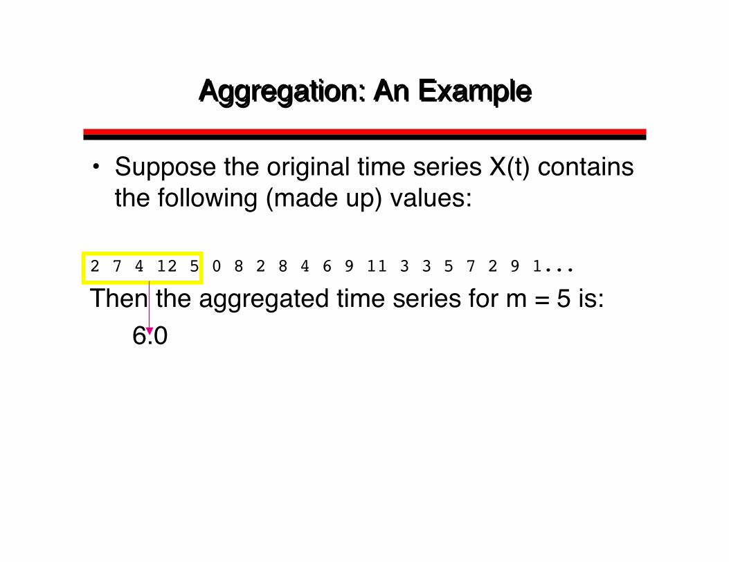
• Suppose the original time series X(t) containsthe following (made up) values:
2 7 4 12 5 0 8 2 8 4 6 9 11 3 3 5 7 2 9 1...
Then the aggregated time series for m = 5 is: 6.0

Aggregation: An ExampleAggregation: An Example
• Suppose the original time series X(t) containsthe following (made up) values:
2 7 4 12 5 0 8 2 8 4 6 9 11 3 3 5 7 2 9 1...
Then the aggregated time series for m = 5 is: 6.0 4.4

Aggregation: An ExampleAggregation: An Example
• Suppose the original time series X(t) containsthe following (made up) values:
2 7 4 12 5 0 8 2 8 4 6 9 11 3 3 5 7 2 9 1...
Then the aggregated time series for m = 5 is: 6.0 4.4 6.4 4.8 ...
Aggregation: An ExampleAggregation: An Example
• Suppose the original time series X(t) containsthe following (made up) values:
2 7 4 12 5 0 8 2 8 4 6 9 11 3 3 5 7 2 9 1...
Then the aggregated time series for m = 10 is:
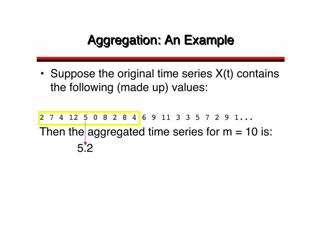
Aggregation: An ExampleAggregation: An Example
• Suppose the original time series X(t) containsthe following (made up) values:
2 7 4 12 5 0 8 2 8 4 6 9 11 3 3 5 7 2 9 1...
Then the aggregated time series for m = 10 is: 5.2
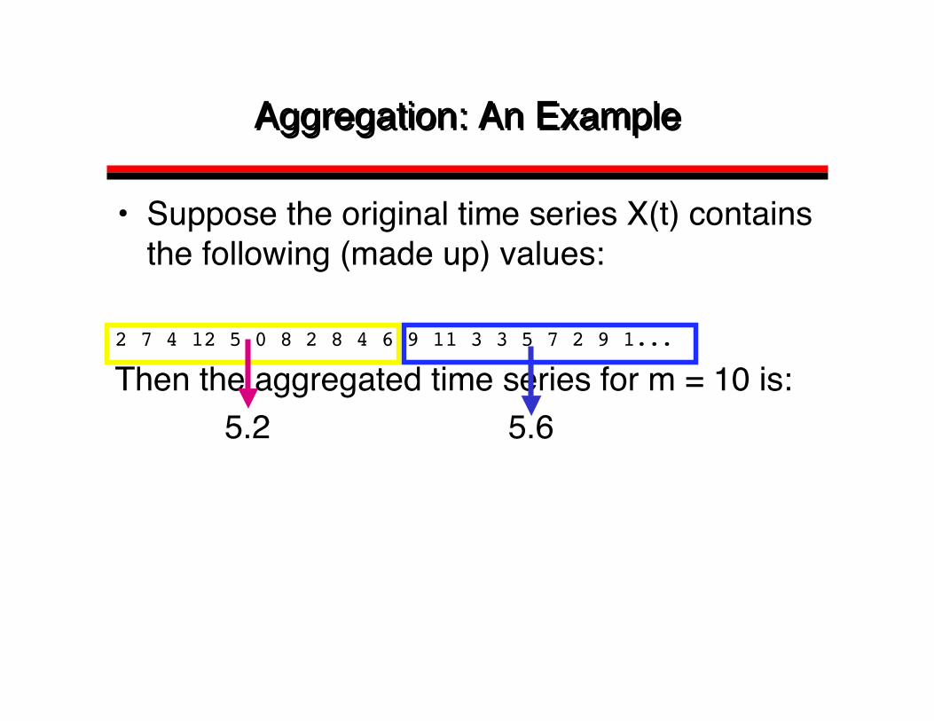
Aggregation: An ExampleAggregation: An Example
• Suppose the original time series X(t) containsthe following (made up) values:
2 7 4 12 5 0 8 2 8 4 6 9 11 3 3 5 7 2 9 1...
Then the aggregated time series for m = 10 is: 5.2 5.6

+1
-1
0
lag k0 100Aut
ocor
rela
tion
Coe
ffic
ient
Original self-similarprocess
Aggregated self-similarprocess
Autocorrelation Function
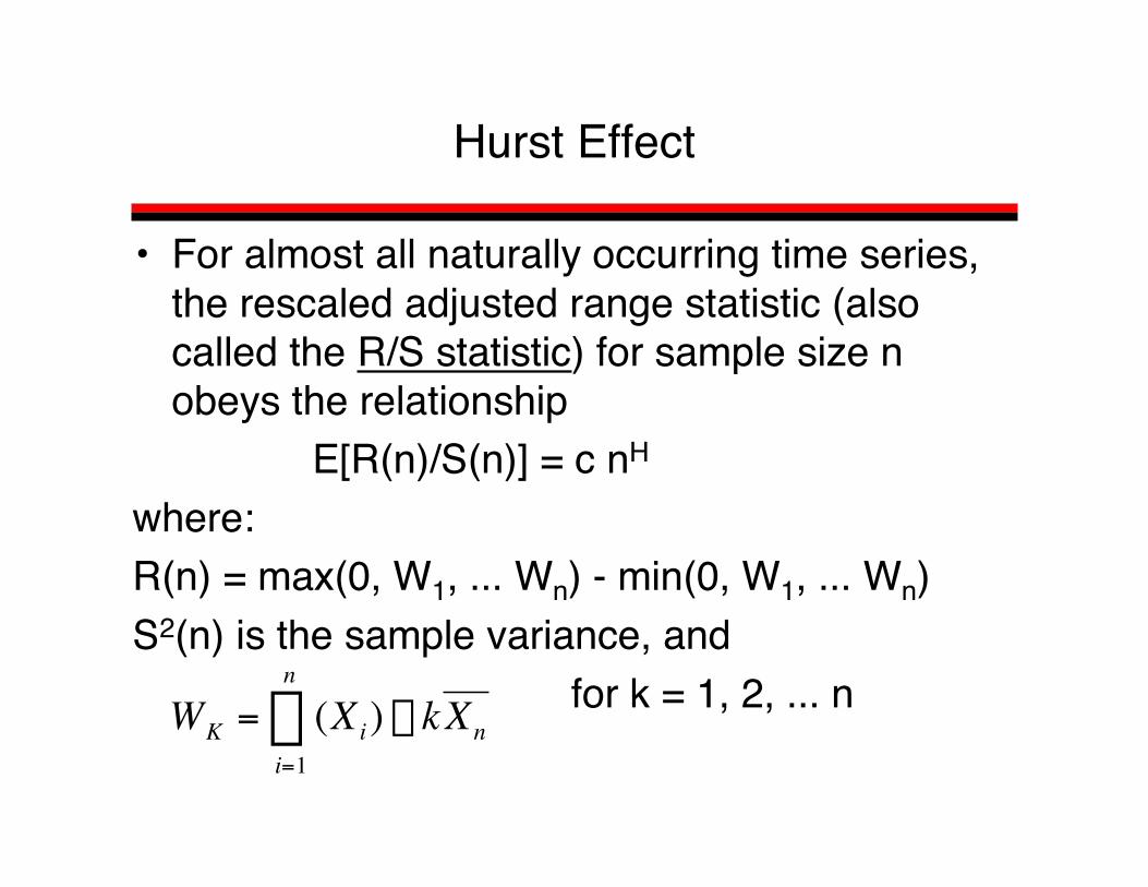
• For almost all naturally occurring time series,the rescaled adjusted range statistic (alsocalled the R/S statistic) for sample size nobeys the relationship
E[R(n)/S(n)] = c nH
where:R(n) = max(0, W1, ... Wn) - min(0, W1, ... Wn)S2(n) is the sample variance, and for k = 1, 2, ... n
†
WK = (Xi) - k Xni=1
n
Â
Hurst Effect
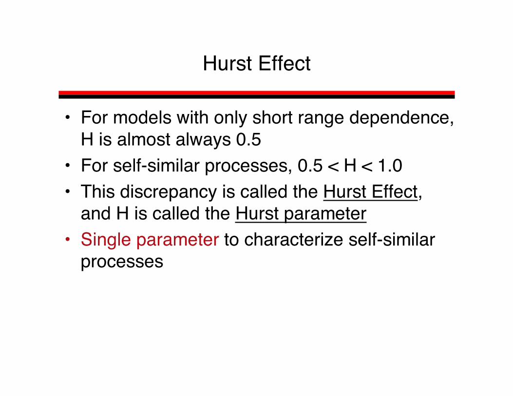
• For models with only short range dependence,H is almost always 0.5
• For self-similar processes, 0.5 < H < 1.0• This discrepancy is called the Hurst Effect,
and H is called the Hurst parameter• Single parameter to characterize self-similar
processes
Hurst Effect
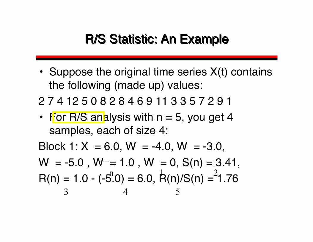
R/S Statistic: An ExampleR/S Statistic: An Example
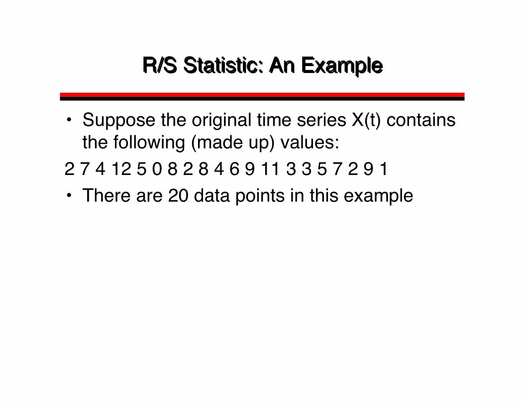
• Suppose the original time series X(t) containsthe following (made up) values:
2 7 4 12 5 0 8 2 8 4 6 9 11 3 3 5 7 2 9 1• There are 20 data points in this example

R/S Statistic: An ExampleR/S Statistic: An Example
• Suppose the original time series X(t) containsthe following (made up) values:
2 7 4 12 5 0 8 2 8 4 6 9 11 3 3 5 7 2 9 1• There are 20 data points in this example• For R/S analysis with n = 1, you get 20
samples, each of size 1:
R/S Statistic: An ExampleR/S Statistic: An Example
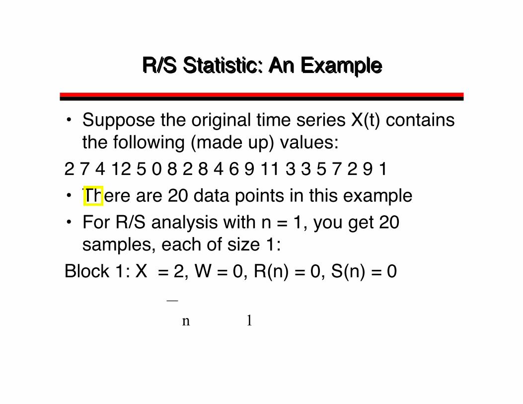
• Suppose the original time series X(t) containsthe following (made up) values:
2 7 4 12 5 0 8 2 8 4 6 9 11 3 3 5 7 2 9 1• There are 20 data points in this example• For R/S analysis with n = 1, you get 20
samples, each of size 1:Block 1: X = 2, W = 0, R(n) = 0, S(n) = 0
n 1

R/S Statistic: An ExampleR/S Statistic: An Example
• Suppose the original time series X(t) containsthe following (made up) values:
2 7 4 12 5 0 8 2 8 4 6 9 11 3 3 5 7 2 9 1• There are 20 data points in this example• For R/S analysis with n = 1, you get 20
samples, each of size 1:Block 2: X = 7, W = 0, R(n) = 0, S(n) = 0
n 1

R/S Statistic: An ExampleR/S Statistic: An Example
• Suppose the original time series X(t) containsthe following (made up) values:
2 7 4 12 5 0 8 2 8 4 6 9 11 3 3 5 7 2 9 1• For R/S analysis with n = 2, you get 10
samples, each of size 2:
R/S Statistic: An ExampleR/S Statistic: An Example
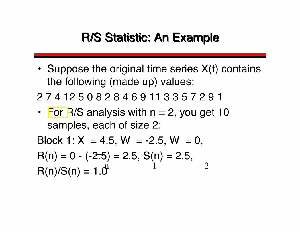
• Suppose the original time series X(t) containsthe following (made up) values:
2 7 4 12 5 0 8 2 8 4 6 9 11 3 3 5 7 2 9 1• For R/S analysis with n = 2, you get 10
samples, each of size 2:Block 1: X = 4.5, W = -2.5, W = 0,R(n) = 0 - (-2.5) = 2.5, S(n) = 2.5,R(n)/S(n) = 1.0n 1 2
R/S Statistic: An ExampleR/S Statistic: An Example
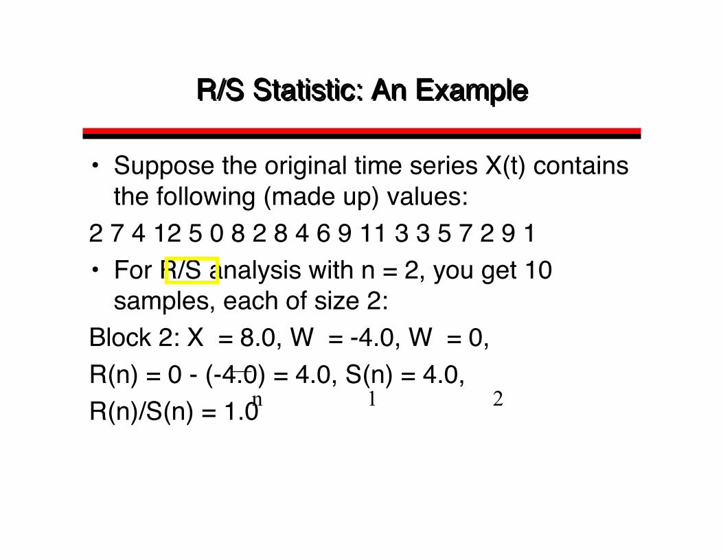
• Suppose the original time series X(t) containsthe following (made up) values:
2 7 4 12 5 0 8 2 8 4 6 9 11 3 3 5 7 2 9 1• For R/S analysis with n = 2, you get 10
samples, each of size 2:Block 2: X = 8.0, W = -4.0, W = 0,R(n) = 0 - (-4.0) = 4.0, S(n) = 4.0,R(n)/S(n) = 1.0n 1 2

R/S Statistic: An ExampleR/S Statistic: An Example
• Suppose the original time series X(t) containsthe following (made up) values:
2 7 4 12 5 0 8 2 8 4 6 9 11 3 3 5 7 2 9 1• For R/S analysis with n = 3, you get 6
samples, each of size 3:
R/S Statistic: An ExampleR/S Statistic: An Example
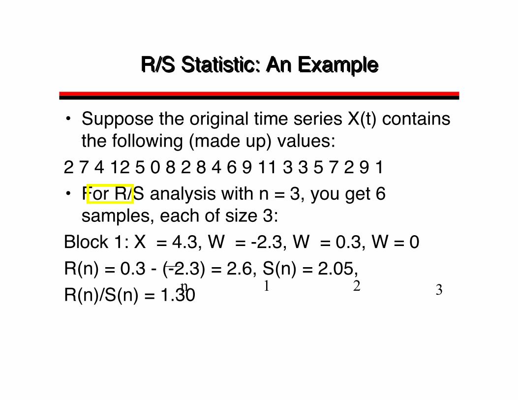
• Suppose the original time series X(t) containsthe following (made up) values:
2 7 4 12 5 0 8 2 8 4 6 9 11 3 3 5 7 2 9 1• For R/S analysis with n = 3, you get 6
samples, each of size 3:Block 1: X = 4.3, W = -2.3, W = 0.3, W = 0R(n) = 0.3 - (-2.3) = 2.6, S(n) = 2.05,R(n)/S(n) = 1.30n 1 2 3
R/S Statistic: An ExampleR/S Statistic: An Example
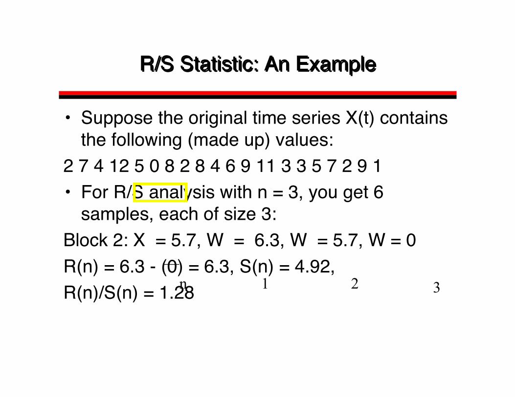
• Suppose the original time series X(t) containsthe following (made up) values:
2 7 4 12 5 0 8 2 8 4 6 9 11 3 3 5 7 2 9 1• For R/S analysis with n = 3, you get 6
samples, each of size 3:Block 2: X = 5.7, W = 6.3, W = 5.7, W = 0R(n) = 6.3 - (0) = 6.3, S(n) = 4.92,R(n)/S(n) = 1.28n 1 2 3
R/S Statistic: An ExampleR/S Statistic: An Example
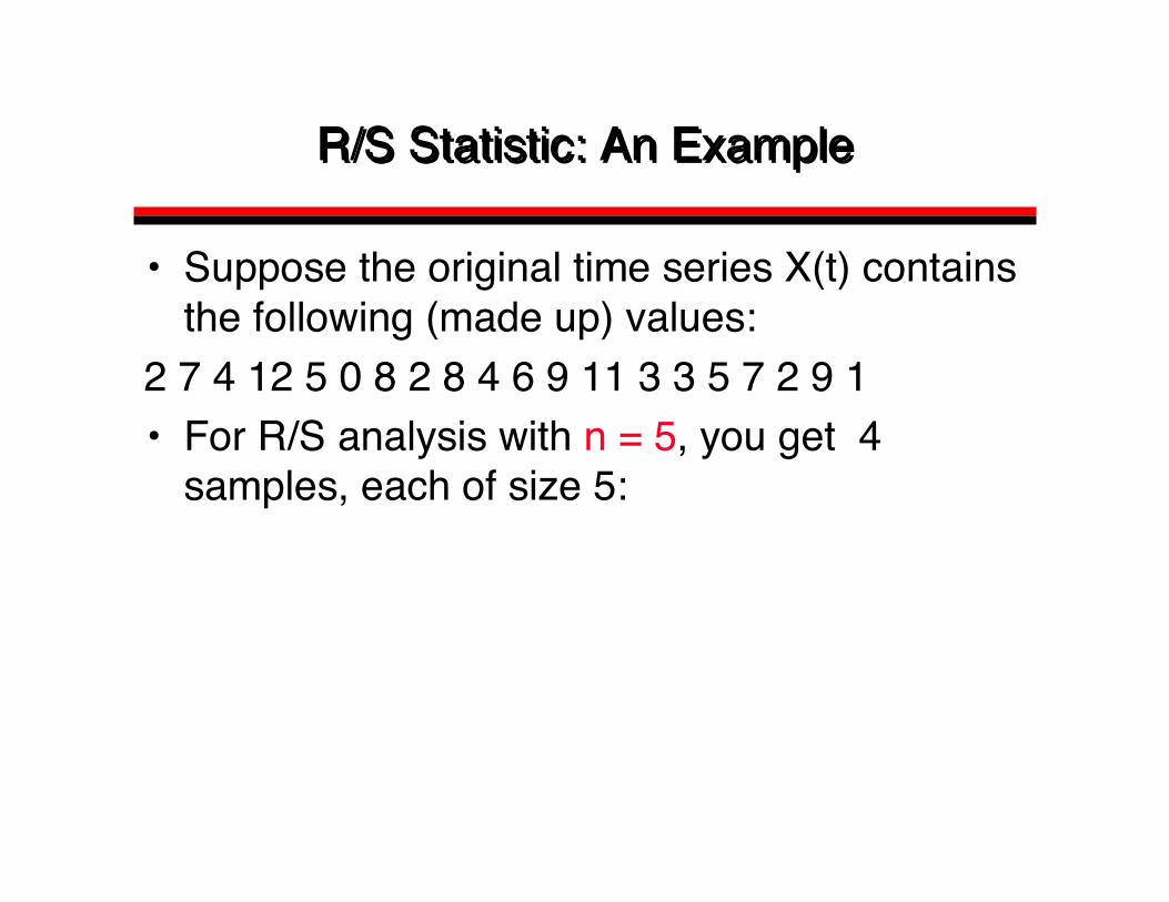
• Suppose the original time series X(t) containsthe following (made up) values:
2 7 4 12 5 0 8 2 8 4 6 9 11 3 3 5 7 2 9 1• For R/S analysis with n = 5, you get 4
samples, each of size 5:
R/S Statistic: An ExampleR/S Statistic: An Example
• Suppose the original time series X(t) containsthe following (made up) values:
2 7 4 12 5 0 8 2 8 4 6 9 11 3 3 5 7 2 9 1• For R/S analysis with n = 5, you get 4
samples, each of size 4:Block 1: X = 6.0, W = -4.0, W = -3.0,W = -5.0 , W = 1.0 , W = 0, S(n) = 3.41,R(n) = 1.0 - (-5.0) = 6.0, R(n)/S(n) = 1.76n 1 2
3 4 5
R/S Statistic: An ExampleR/S Statistic: An Example
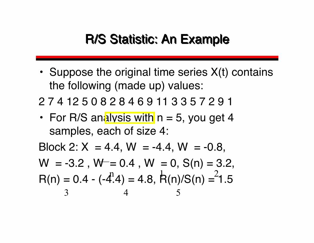
• Suppose the original time series X(t) containsthe following (made up) values:
2 7 4 12 5 0 8 2 8 4 6 9 11 3 3 5 7 2 9 1• For R/S analysis with n = 5, you get 4
samples, each of size 4:Block 2: X = 4.4, W = -4.4, W = -0.8,W = -3.2 , W = 0.4 , W = 0, S(n) = 3.2,R(n) = 0.4 - (-4.4) = 4.8, R(n)/S(n) = 1.5n 1 2
3 4 5

R/S Statistic: An ExampleR/S Statistic: An Example
• Suppose the original time series X(t) containsthe following (made up) values:
2 7 4 12 5 0 8 2 8 4 6 9 11 3 3 5 7 2 9 1• For R/S analysis with n = 10, you get 2
samples, each of size 10:
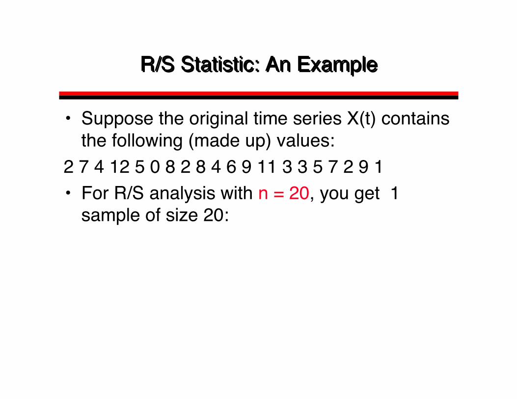
R/S Statistic: An ExampleR/S Statistic: An Example
• Suppose the original time series X(t) containsthe following (made up) values:
2 7 4 12 5 0 8 2 8 4 6 9 11 3 3 5 7 2 9 1• For R/S analysis with n = 20, you get 1
sample of size 20:

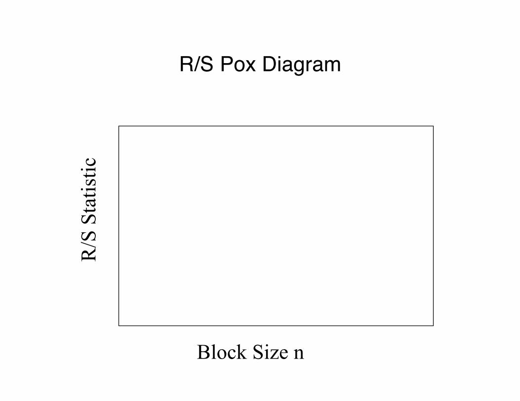
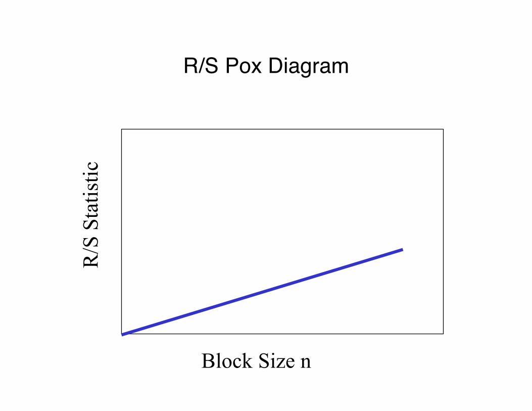
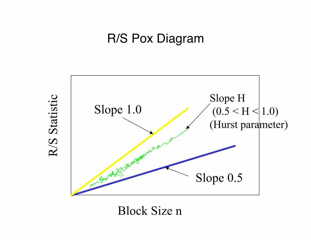
• Another way of testing for self-similarity, andestimating the Hurst parameter
• Plot the R/S statistic for different values of n,with a log scale on each axis
• If time series is self-similar, the resulting plotwill have a straight line shape with a slope Hthat is greater than 0.5
• Called an R/S plot, or R/S pox diagram
R/S Plot
R/S
Sta
tistic
Block Size n
R/S Pox Diagram

R/S
Sta
tistic
Block Size n
R/S statistic R(n)/S(n)on a logarithmic scale
R/S Pox Diagram

R/S
Sta
tistic
Block Size n
Sample size non a logarithmic scale
R/S Pox Diagram
R/S
Sta
tistic
Block Size n
R/S Pox Diagram

R/S
Sta
tistic
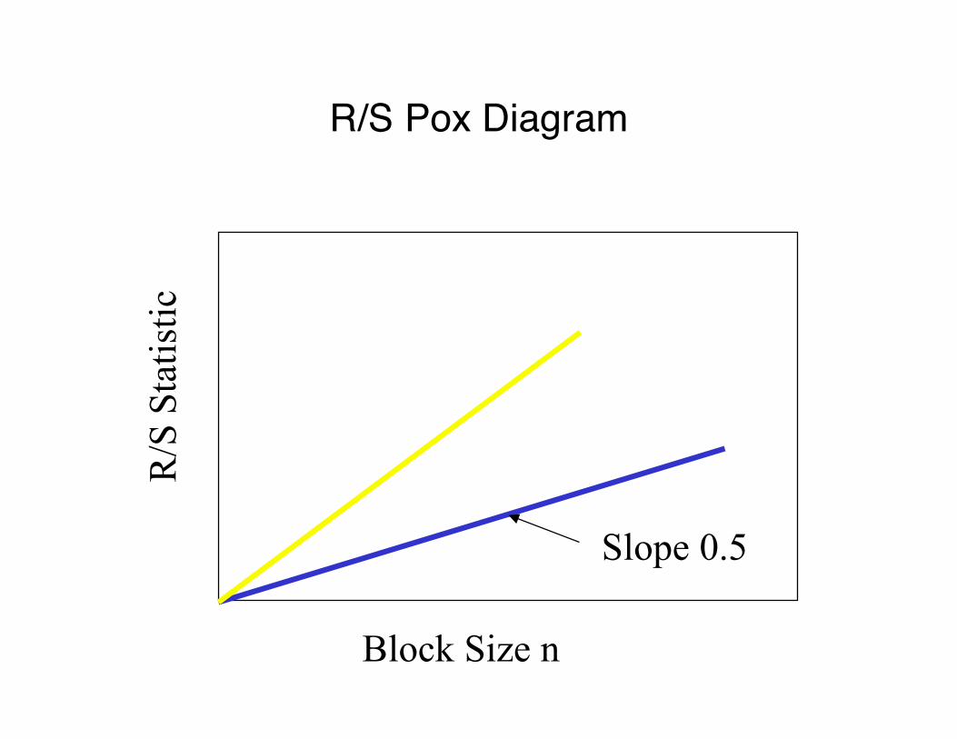
Block Size n
Slope 0.5
R/S Pox Diagram
R/S
Sta
tistic
Block Size n
Slope 0.5
R/S Pox Diagram
R/S
Sta
tistic
Block Size n
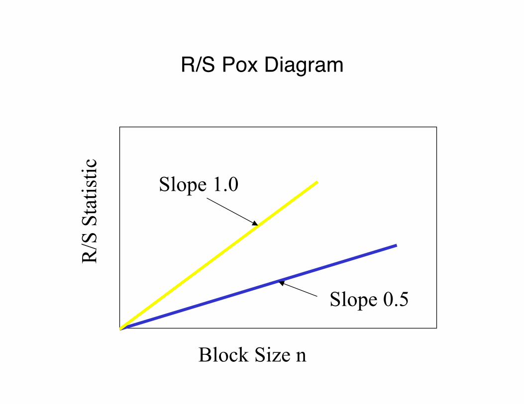
Slope 0.5
Slope 1.0
R/S Pox Diagram

R/S
Sta
tistic
Block Size n
Slope 0.5
Slope 1.0
R/S Pox Diagram
R/S
Sta
tistic
Block Size n
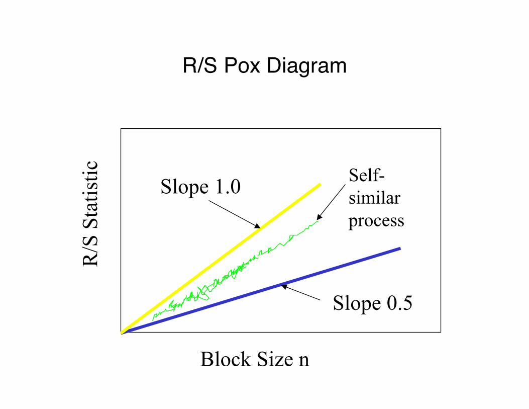
Slope 0.5
Slope 1.0Self-similarprocess
R/S Pox Diagram
R/S
Sta
tistic
Block Size n
Slope 0.5
Slope 1.0Slope H (0.5 < H < 1.0)(Hurst parameter)
R/S Pox Diagram
• Self-similarity is an important mathematicalproperty that has recently been identified aspresent in network traffic measurements
• Important property: burstiness across manytime scales, traffic does not aggregate well
• There exist several mathematical methods totest for the presence of self-similarity, and toestimate the Hurst parameter H
• There exist models for self-similar traffic
Self-Similarity Summary
Newer Results
V. Paxson, S. Floyd, Wide-Area Traffic: The Failure ofPoisson Modeling, IEEE/ACM Transaction on Networking,1995.
• TCP session arrivals are well modeled by a Poissonprocess
• A number of WAN characteristics were well modeled byheavy tailed distributions
• Packet arrival process for two typical applications (TELNET,FTP) as well as aggregate traffic is self-similar
Another Study
M. Crovella, A. Bestavros, Self-Similarity in World WideWeb Traffic: Evidence and Possible Causes,IEEE/ACM Transactions on Networking, 1997
• Analyzed WWW logs collected at clients over a 1.5month period– First WWW client study– Instrumented MOSAIC
• ~600 students• ~130K files transferred• ~2.7GB data transferred
Self-Similar Aspects of Web traffic
• One difficulty in the analysis was finding stationary,busy periods– A number of candidate hours were found
• All four tests for self-similarity were employed– 0.7 < H < 0.8
Explaining Self-Similarity
• Consider a set of processes which are eitherON or OFF– The distribution of ON and OFF times are heavy
tailed– The aggregation of these processes leads to a
self-similar process• So, how do we get heavy tailed ON or OFF
times?

• Analysis of client logs showed that ON times were, in fact,heavy tailed– Over about 3 orders of magnitude
• This lead to the analysis of underlying file sizes– Over about 4 orders of magnitude– Similar to FTP traffic
• Files available from UNIX file systems are typically heavy tailed
Impact of File Sizes
Heavy Tailed OFF times
• Analysis of OFF times showed that they arealso heavy tailed
• Distinction between Active and Passive OFFtimes– Inter vs. Intra click OFF times
• Thus, ON times are more likely to be cause ofself-similarity

Major Results from CB97
• Established that WWW traffic was self-similar• Modeled a number of different WWW
characteristics (focus on the tail)• Provide an explanation for self-similarity of WWW
traffic based on underlying file size distribution
Where are we now?
• There is no mechanistic model for Internet traffic– Topology?– Routing?
• People want to blame the protocols for observed behavior• Multiresolution analysis may provide a means for better
models• Many people (vendors) chose to ignore self-similarity
– Does it matter????– Critical opportunity for answering this question.


