Queuing Theory - unisi.it · MS&E 121 Handout #25 Introduction to Stochastic Processes & Models...

MS&E 121 Handout #25 Introduction to Stochastic Processes & Models February 19, 2002

Queuing Theory

Overview of Queuing Theory Lectures

Introduction to Queueing Systems– Important Questions about Queueing Systems– Components of a Queuing System

Fundamental Results for General Queueing Systems– Terminology for General Queueing Systems– Steady State Quantities– Fundamental Quantities of Interest– Basic Cost Identity– Consequences: Little’s Law and Other Useful Relationships

Properties of Poisson Arrival Processes– Superposition and decomposition of Poisson arrivals– Poisson arrivals see time averages


Overview of Queuing Theory Lectures, continued

Queueing Systems with Exponential Arrivals and Service – M/M/1 queue– M/M/S queue – M/M/1/C queue – Markovian queues with general state definition

Networks of Markovian Queues– The Equivalence Property– Open Jackson networks – Closed Jackson networks

Queueing Systems with Nonexponential Distributions– The M/G/1 Queue– Special Cases of M/G/1: M/D/1 and M/Ek/1 queues

examples: security checkpointSafeway checkout linestwo law practicesStanford post officeshoeshine shop

examples: car washWard’s Berry Farmroommate network

examples: McDonald’s Drive Thruhomework questions

Important Questions about Queueing Systems

• What fraction of time is each server idle?

• What is the expected number of customers in the queue? in the queue plus in service?

• What is the probability distribution of the number of customers in the queue? in the queue plus in service?

• What is the expected time that each customer spends in the queue? in the queue plus in service?

• What is the probability distribution of a customer’s waiting time in the queue? in the queue plus in service?


Components of a Queueing System

queueserved

customerscustomers

Arrival Process Queue Service Process

input source

service mechanism

Components of a Queueing System: The Arrival Process

input source

service mechanismqueue

served customers

customers

Characteristics of Arrival Process:• finite or infinite calling population• bulk or individual arrivals• interarrival time distribution• simple or compound arrival processes• balking or no balking


Components of a Queueing System: The Queue

queueinput

sourcecustomers service

mechanismserved

customers

Queue Characteristics:

• finite or infinite• queue discipline:

FCFS = first-come-first-served LCFS = last -come-first-servedPriority service order Random service order

Components of a Queueing System: The Service Process

input source

service mechanismqueue

served customers

customers

Characteristics of Service Process:• number/configurations of servers• batch or single service• service time distribution• rework


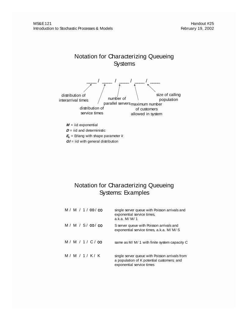
Notation for Characterizing Queueing Systems

____ / ____ / ____ / ____ / ____

distribution of interarrival times

distribution of service times

number of parallel servers maximum number

of customers allowed in system

size of calling population

M = iid exponentialD = iid and deterministicEk = Erlang with shape parameter kGI = iid with general distribution

Notation for Characterizing Queueing Systems: Examples

single server queue with Poisson arrivals and exponential service times, a.k.a. M/M/1

same as M/M/1 with finite system capacity C

S server queue with Poisson arrivals and exponential service times, a.k.a. M/M/S

M / M / 1 / /∞ ∞

M / M / 1 / C /∞

M / M / S / /∞ ∞

M / M / 1 / K / K single server queue with Poisson arrivals from a population of K potential customers; and exponential service times


Terminology for General Queueing Systems

N(t) = the number of customers in the system at time t: this includes both customers that are in the queue and being served

Pn(t) = the probability that there are exactly n customers in the system at time t

= P(N(t)=n)

λn = mean arrival rate of entering customers when n customers are in the system

µn = mean service rate for overall system when n customers are in the system

Note: N(t) and Pn(t) are difficult to compute for general t. We will be mainly interested in their values as t becomes infinite.

Steady State Quantities

Pn = long run probability that there will be exactly n customers in the system

= lim ( )t

nP t→∞

λ = long run average arrival rate of entering customers

= Pnn

n=

∞

�0

λ

For general queues, the steady state probabilities Pn can be difficult to compute.However, if the queue is a continuous time Markov Chain, then Pn= ωn (if a steady-state distribution exists).


Fundamental Quantities of Interest

L = the long run average number of customers in the system

LQ = the long run average number of customers waiting in queue

LS = the long run average number of customers in service

L = LS + LQ

More Fundamental Quantities of Interest

W = the waiting time in the system for an arbitrary customer (random variable)

WQ = the waiting time in the queue for an arbitrary customer (random variable)

W = the long run average amount of time a customer spends in the system

= E(W )

WQ= the long run average amount of time a customer spends in the queue

= E(WQ )

WS = the long run average amount of time a customer spends in service

W = WS + WQ


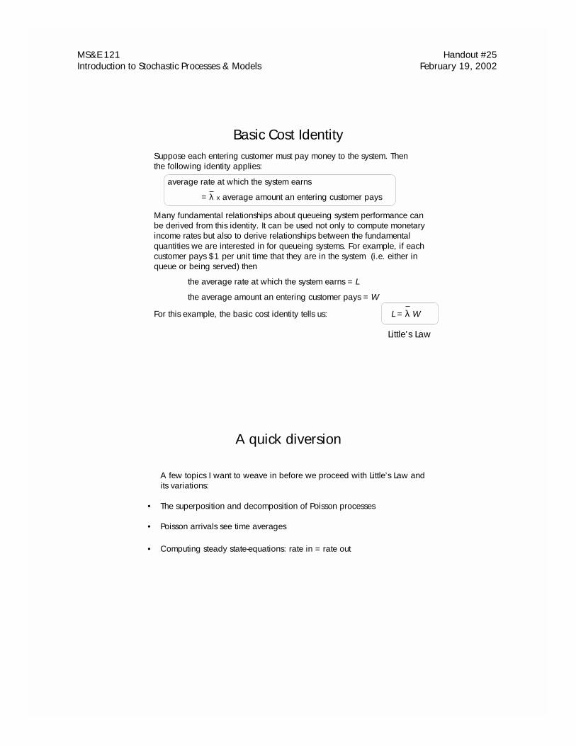
Basic Cost Identity

average rate at which the system earns

= λ x average amount an entering customer pays

Suppose each entering customer must pay money to the system. Then the following identity applies:

Many fundamental relationships about queueing system performance can be derived from this identity. It can be used not only to compute monetary income rates but also to derive relationships between the fundamental quantities we are interested in for queueing systems. For example, if each customer pays $1 per unit time that they are in the system (i.e. either in queue or being served) then

the average rate at which the system earns = L

the average amount an entering customer pays = W

For this example, the basic cost identity tells us: L = λ W

Little’s Law

A quick diversion

A few topics I want to weave in before we proceed with Little’s Law and its variations:

• The superposition and decomposition of Poisson processes

• Poisson arrivals see time averages

• Computing steady state-equations: rate in = rate out


Superposition of Poisson Arrival Processes

Often the arrival process to a queue consists of multiple different arrival processes of customers from different origins. It turns out that it is easy to deal with such compound arrival processes when each individual arrival process is Poisson and is independent of the others.

Suppose you have two independent Poisson arrival processes X and Y with respective rates λx and λy. Then the combination of the two arrival streams is also a Poisson process with rate λx+λy.

Why? Let T be a random variable representing the remaining time until an arrival of either type occurs. Let Tx and Ty be the remaining times until arrivals of type x and y occur. Then T = min{Tx,Ty}. Since Tx and Ty are exponentially distributed with parameters λx and λy respectively, T must also be exponentially distributed with parameter λx+λy. Hence, the combined stream has exponential interarrival times, and is thus a Poisson process with rate λx+λy.

Decomposition of Poisson Arrival Processes

Another nice property of Poisson arrival processes allows us to disaggregate the process into independent Poisson processes. Suppose customers arrive to our system according to a Poisson process with rate λ. Suppose that an arriving customer is of type k with probability pk, where

Then the arrivals of customers of type k follow a Poisson process with rate pkλ.

An example: suppose arriving customers to a system balk with fixed probability p independent of the number of people in the system. If the arrival process is Poisson with rate λ, the arrivals who stay follow a Poisson process with rate (1-p)λ. The customers who balk do so according to a Poisson process with rate pλ.

.11

�=

=n

kkp


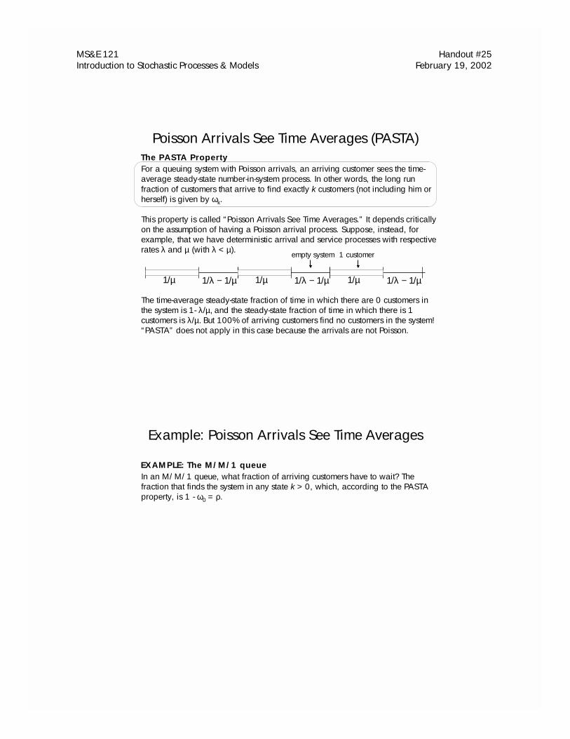
Poisson Arrivals See Time Averages (PASTA)

For a queuing system with Poisson arrivals, an arriving customer sees the time-average steady-state number-in-system process. In other words, the long run fraction of customers that arrive to find exactly k customers (not including him or herself) is given by ωk.

This property is called “Poisson Arrivals See Time Averages.” It depends critically on the assumption of having a Poisson arrival process. Suppose, instead, for example, that we have deterministic arrival and service processes with respective rates λ and µ (with λ < µ).

The time-average steady-state fraction of time in which there are 0 customers in the system is 1- λ/µ, and the steady-state fraction of time in which there is 1 customers is λ/µ. But 100% of arriving customers find no customers in the system! “PASTA” does not apply in this case because the arrivals are not Poisson.

The PASTA Property

1/µ 1/λ − 1/µ 1/µ 1/λ − 1/µ 1/µ 1/λ − 1/µ

empty system 1 customer

Example: Poisson Arrivals See Time Averages

In an M/M/1 queue, what fraction of arriving customers have to wait? The fraction that finds the system in any state k > 0, which, according to the PASTA property, is 1 - ω0 = ρ.

EXAMPLE: The M/M/1 queue


Computing the steady state distribution: Rate In = Rate Out

When studying CTMCs, we learned that each of the steady state equations

could be expressed as:

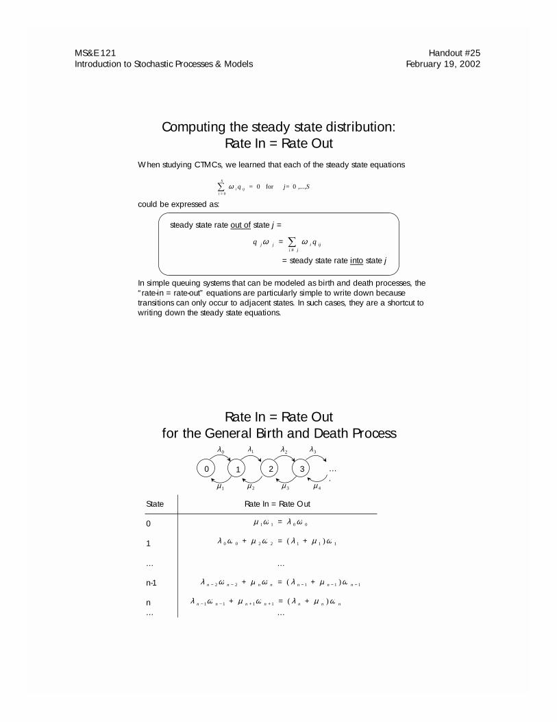
In simple queuing systems that can be modeled as birth and death processes, the “rate-in = rate-out” equations are particularly simple to write down because transitions can only occur to adjacent states. In such cases, they are a shortcut to writing down the steady state equations.

,...,Sj=qS

iiji 0for0=

0�

=

ω

�≠

=ji

ijijj qq ωω

steady state rate out of state j =

= steady state rate into state j

Rate In = Rate Out for the General Birth and Death Process

State Rate In = Rate Out

0

1

... ...

n-1

n... ...

0011 ωλωµ =

0 1 2 3 ….

λ 0

µ 1

λ1 λ 2 λ 3

µ 2 µ 3 µ 4

1112200 )( ωµλωµωλ +=+

11122 )( −−−−− +=+ nnnnnnn ωµλωµωλ

nnnnnnn ωµλωµωλ )(1111 +=+ ++−−


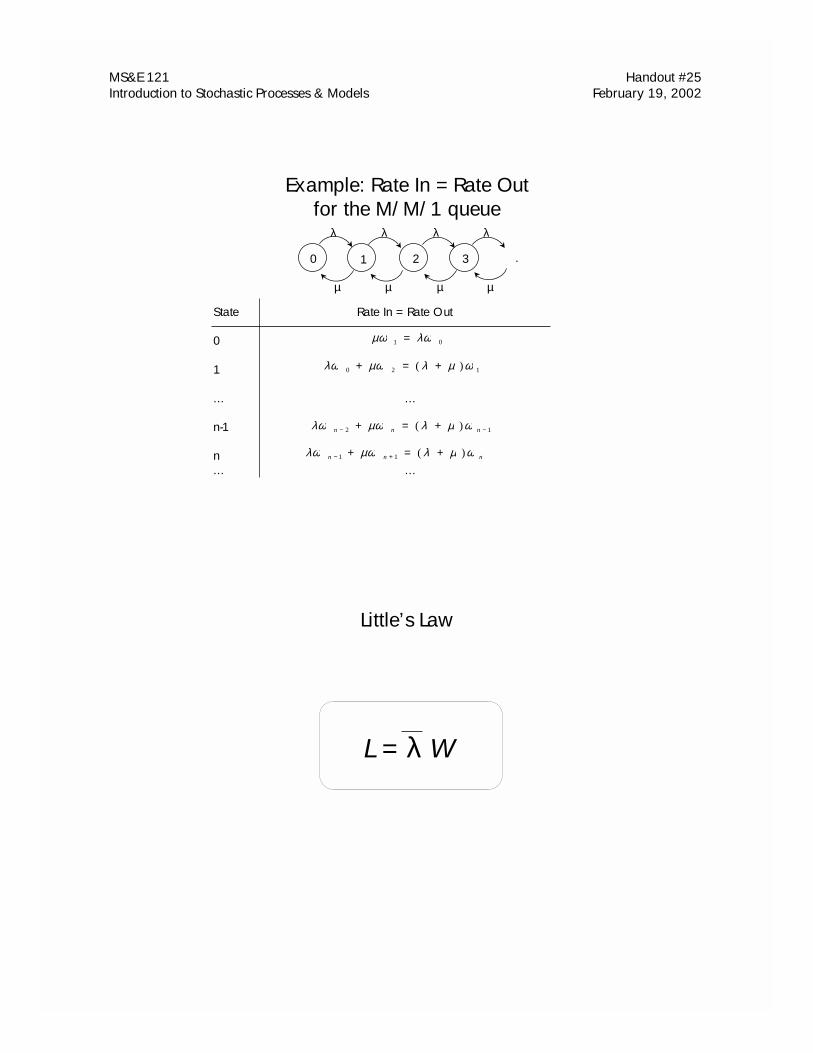
Example: Rate In = Rate Out for the M/M/1 queue

State Rate In = Rate Out

0

1

... ...

n-1

n... ...

01 λωµω =

120 )( ωµλµωλω +=+

12 )( −− +=+ nnn ωµλµωλω

nnn ωµλµωλω )(11 +=+ +−

0 1 2 3 .

µ µ µ µ

λ λ λ λ

Little’s Law

L = λ W


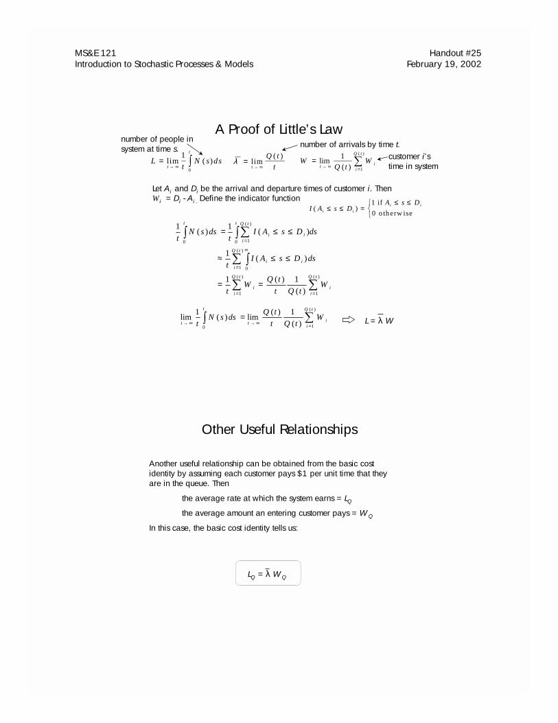
A Proof of Little’s Law

��

� �

� ��

==

=

∞

=

==

≤≤≈

≤≤=

)(

1

)(

1

)(

1 0

0

)(

10

)(

1)(1

)(1

)(1

)(1

tQ

ii

tQ

ii

tQ

iii

t tQ

iii

t

tQt

tQ

t

dsDsAIt

dsDsAIt

dssNt

WW

��=∞→∞→

=)(

10 )(

1)(lim)(

1lim

tQ

ii

t

t

t tQt

tQdssN

tW L = λ W

Lt

N s dst

t

=→ ∞ �lim ( )

1

0

λ =→ ∞

lim( )

t

Q t

t �=∞→

=)(

1)(

1lim

tQ

ii

t tQW W customer i’s

time in system

Let Ai and Di be the arrival and departure times of customer i. ThenWi = Di - Ai . Define the indicator function

number of arrivals by time t.

I A s DA s D

i i

i i( )≤ ≤ =

≤ ≤��

1

0

if

o th erw ise

number of people in system at time s.

Other Useful Relationships

Another useful relationship can be obtained from the basic cost identity by assuming each customer pays $1 per unit time that they are in the queue. Then

the average rate at which the system earns = LQ

the average amount an entering customer pays = WQ

In this case, the basic cost identity tells us:

LQ = λ WQ


Other Useful Relationships

By assuming instead that each customer pays $1 per unit time that they are in service, we have

the average rate at which the system earns = LS

the average amount an entering customer pays = WS

The basic cost identity amounts to:

LS = λ WS

Exponential Queuing Models

We now show how to apply these results to queues having exponentially distributed interarrival times and service times. These types of queues are the most tractable mathematically.

Some of the queues we’ll look at:

M/M/1

M/M/S

M/M/1/C (finite capacity C)

Queues with more general state definition


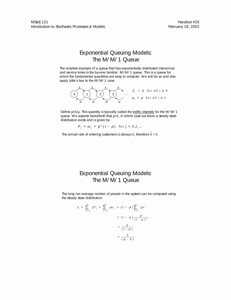
Exponential Queuing Models: The M/M/1 Queue

0 1 2 3 ….

µ µ µ µ

λ λ λ λλ λi i= f o r a l l ≥ 0

µ µi i= ≥f o r a l l 1

The simplest example of a queue that has exponentially distributed interarrival and service times is the by-now familiar M/M/1 queue. This is a queue for which the fundamental quantities are easy to compute. We will do so and also apply Little’s law to the M/M/1 case.

Define ρ=λ/µ. This quantity is typically called the traffic intensity for the M/M/1 queue. We assume henceforth that ρ<1, in which case we know a steady state distribution exists and is given by:

P jj jj= = − =ω ρ ρ( ) , , . . .1 0 1fo r

The arrival rate of entering customers is always λ; therefore λ = λ.


The long run average number of people in the system can be computed using the steady state distribution:

L j P j jj

jj

jj

j

= = = −=

∞

=

∞

=

∞

� � �0 0 0

1ω ρ ρ( )

= −( ))

1 2ρ ρρ( 1 -

= ρρ( 1 - )

= λµ λ( - )



We can also compute the long run expected number of customers in the queue LQ using the steady state distribution as follows:

L j P j jQj

jj

jj

j jj

= − = − = −=

∞

=

∞

=

∞

=

∞

� � � �( ) ( )1 11 1 1 1

ω ω ω

= − =λµ λ

λµ

λµ µ λ( - ( -) )

2

= − −=

∞

� jj

j0

01ω ω( )

= −L ρ

L S jj

= ⋅ + ⋅ = − = ==

∞

�0 1 101

0ω ω ω ρ λµ

The expected number of customers in service LS is

Verify that L = LS + LQ for this example.


The distribution for the waiting time W of an arbitrary customer (in the long run) is computed as follows:

)( aP ≤W arrives)hewhensystemin()arriveshewhensystemin|(0

nPnaPn�

∞

=

≤= W

= + − + ≤=

∞

� P n a Pn

n( ( ) )service times of person in service waiting him10

= ⋅−

=

∞

�� µµ

ρ ρµe( t)

n!dt ( - )t

a

n

nn

00

1

= − −

=

∞

� �( )µ λλµe

( t)

n!dtt

a n

n0 0

= − −� ( )µ λ µ λe e dtt

a

t

0

= − − −1 e a( )µ λ

(sum of n+1 iid exponential random variables with parameter µ has an Erlang distribution with parameters (µ/(n+1), n+1) (akagamma (n+1,µ))

(interchanging the sum and the integral)

(using the identity )( t)

n !e

n

n

tλ λ

=

∞

� =0

So W is exponentially distributed with parameter (µ−λ)!



Now we’ll derive the distribution for the waiting time in the queue WQ of an arbitrary customer in the long run. Since an arriving customer who find no customers in the queue has no wait, ρ−=== 1)0( 0PP QW

arrives)hewhensystemin()arriveshewhensystemin|()(1

nPnaPaPn

QQ �∞

=

>=> WW

= + − >=

∞

� P n a Pn

n( ( ) )service times of person in service waiting11

=−

⋅−∞

=

∞ −

�� µµ

ρ ρµe( t)

n !dt ( - )t

an

nn

1

1

11

( )

=−

−−

∞ −

=

∞

� �λ µ λ

µλµ( )

( )e

( t)

n !d tt

a

n

n

1

1 1

=− −

∞

�λ µ λ

µµ λ( )

e e dtt

a

t

= − −ρ µ λe a( )

WQ is not exponentially distributed, but the conditional distribution of WQ, given that WQ>0, is! To see this...

a

Q

QQQ e

P

aPaP )(

)0(

)()0|( λµ −−=

>>

=>>W

WWW


Let’s now compute W, the expected time a customer spends in the system, first using Little’s Law:

The expected time a customer spends in the service is:

Evidently W = WS + WQ for this example.

Using LQ = λ WQ we can compute the expected time a customer spends in the queue:

It is easy to verify that we get the same result by taking the expected value of W.

Verify by taking the expected value of WQ !

WL L

= = =−

⋅ =−λ λ

λµ λ λ µ λ

1 1

WL L

Q

Q Q= = =−

⋅ =−λ λ

λµ µ λ λ

λµ µ λ

2 1

( ) ( )

WL

SS= = =λ

λµ λ µ

1 1 obvious!


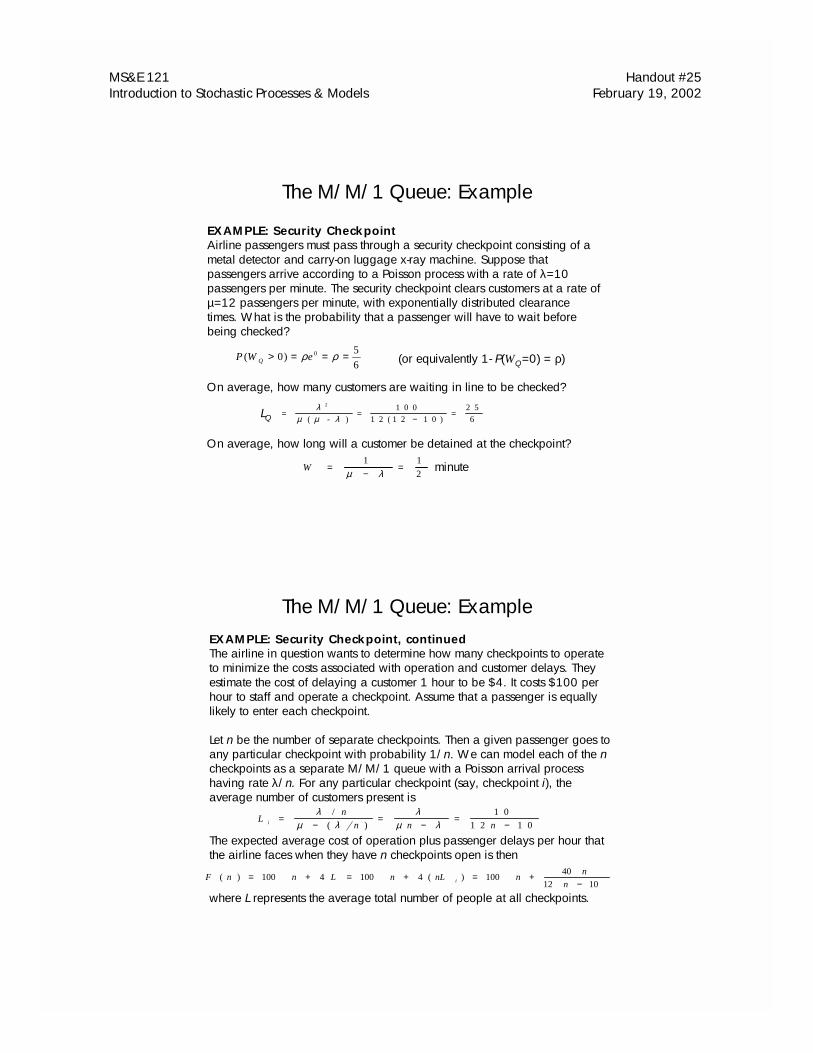
The M/M/1 Queue: Example

EXAMPLE: Security CheckpointAirline passengers must pass through a security checkpoint consisting of a metal detector and carry-on luggage x-ray machine. Suppose that passengers arrive according to a Poisson process with a rate of λ=10 passengers per minute. The security checkpoint clears customers at a rate of µ=12 passengers per minute, with exponentially distributed clearance times. What is the probability that a passenger will have to wait before being checked?

(or equivalently 1- P(WQ=0) = ρ)

On average, how many customers are waiting in line to be checked?

On average, how long will a customer be detained at the checkpoint?

LQ

6

5)0( 0 ===> ρρeP QW

= =−

=λ

µ µ λ

2 1 0 0

1 2 1 2 1 0

2 5

6( - ) ( )

W =−

=1 1

2µ λ minute

The M/M/1 Queue: ExampleEXAMPLE: Security Checkpoint, continuedThe airline in question wants to determine how many checkpoints to operate to minimize the costs associated with operation and customer delays. They estimate the cost of delaying a customer 1 hour to be $4. It costs $100 per hour to staff and operate a checkpoint. Assume that a passenger is equally likely to enter each checkpoint.

Let n be the number of separate checkpoints. Then a given passenger goes to any particular checkpoint with probability 1/n. We can model each of the n checkpoints as a separate M/M/1 queue with a Poisson arrival process having rate λ/n. For any particular checkpoint (say, checkpoint i), the average number of customers present is

The expected average cost of operation plus passenger delays per hour that the airline faces when they have n checkpoints open is then

where L represents the average total number of people at all checkpoints.

Ln

n n ni =−

=−

=−

λµ λ

λµ λ

/

( )

1 0

1 2 1 0

1012

40100)(41004100)(

−+=+=+=

n

nnnLnLnnF i


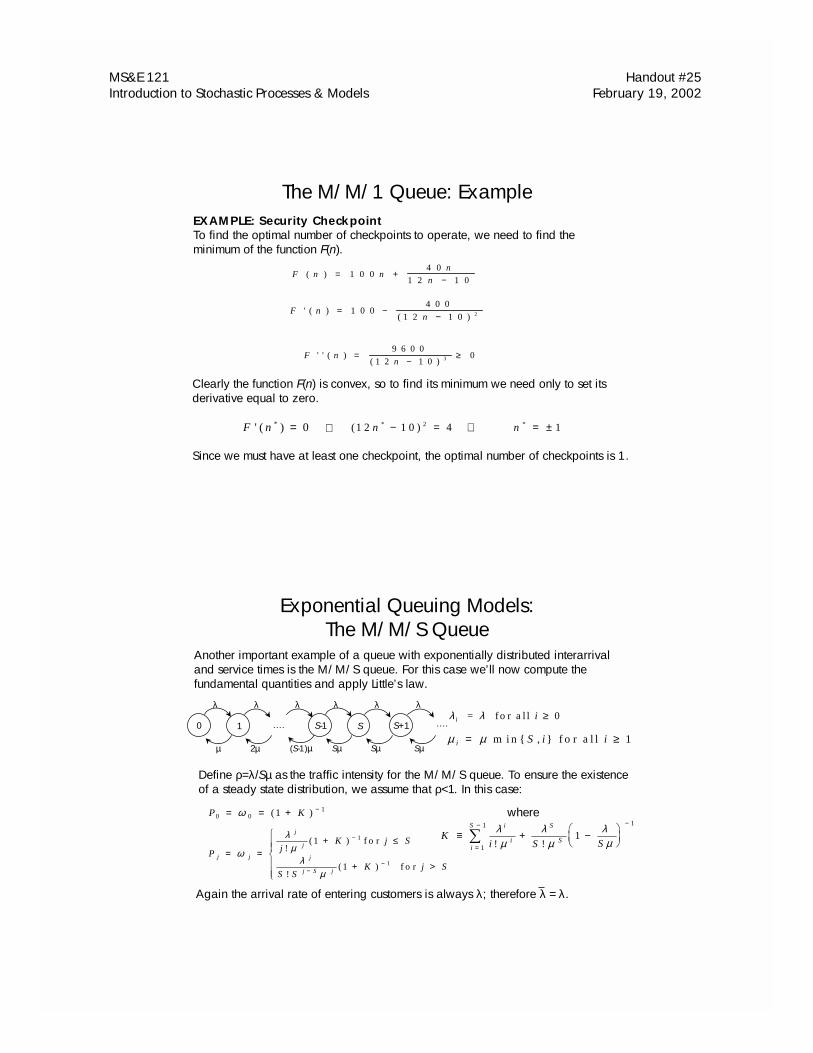
The M/M/1 Queue: ExampleEXAMPLE: Security CheckpointTo find the optimal number of checkpoints to operate, we need to find the minimum of the function F(n).

F n nn

n( ) = +

−1 0 0

4 0

1 2 1 0

F nn

' ( )( )

= −−

1 0 04 0 0

1 2 1 0 2

F nn

' ' ( )( )

=−

≥9 6 0 0

1 2 1 003

Clearly the function F(n) is convex, so to find its minimum we need only to set itsderivative equal to zero.

Since we must have at least one checkpoint, the optimal number of checkpoints is 1.

F n' ( )* = 0 ( )*1 2 1 0 42n − =⇔ ⇔ n * = ± 1

Exponential Queuing Models: The M/M/S Queue

λ λi i= f o r a l l ≥ 0

µ µi S i i= ≥m i n { , } f o r a l l 1….

(S-1)µ

0 1

µ 2µ

λ λ λ

S-1 S S+1….

Sµ Sµ Sµ

λ λ λ

….

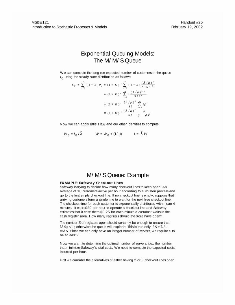
Another important example of a queue with exponentially distributed interarrival and service times is the M/M/S queue. For this case we’ll now compute the fundamental quantities and apply Little’s law.

Again the arrival rate of entering customers is always λ; therefore λ = λ.

Define ρ=λ/Sµ as the traffic intensity for the M/M/S queue. To ensure the existenceof a steady state distribution, we assume that ρ<1. In this case:

P K0 011= = + −ω ( )

Pj

K j S

S SK j S

j j

j

j

j

j S j

= =+ ≤

+ >

�

��

��

−

−−

ω

λµ

λµ

!( )

!( )

1

1

1

1

f o r

f o r

Ki S S

i

ii

S S

S≡ + −�

��

�

��

=

− −

�λµ

λµ

λµ! !1

1 1

1

where


Exponential Queuing Models: The M/M/S Queue

We can compute the long run expected number of customers in the queue LQ using the steady state distribution as follows:

L j S P K j SS SQ

j Sj

j S

j

j S= − = + −=

∞−

=

∞

−� �( ) ( ) ( )( )

!1 1 λ µ

Now we can apply Little’s law and our other identities to compute:

= + −

=

∞ +

�( )( )

!1 1

0

K iS Si

i S

i

λ µ

= + −

=

∞

�( )( )

!1 1

0

KS

iS

i

iλ µρ

= +−

−( )( )

! ( )1

11

2KS

Sλ µ ρρ

WQ = LQ /λ W = WQ + (1/µ) L = λ W

M/M/S Queue: ExampleEXAMPLE: Safeway Checkout LinesSafeway is trying to decide how many checkout lines to keep open. An average of 18 customers arrive per hour according to a Poisson process and go to the first empty checkout line. If no checkout line is empty, suppose that arriving customers form a single line to wait for the next free checkout line. The checkout time for each customer is exponentially distributed with mean 4 minutes. It costs $20 per hour to operate a checkout line and Safeway estimates that it costs them $0.25 for each minute a customer waits in the cash register area. How many registers should the store have open?

The number S of registers open should certainly be enough to ensure that λ/Sµ < 1; otherwise the queue will explode. This is true only if S > λ /µ =6/5. Since we can only have an integer number of servers, we require S to be at least 2.

Now we want to determine the optimal number of servers; i.e., the number that minimize Safeway’s total costs. We need to compute the expected costs incurred per hour.

First we consider the alternatives of either having 2 or 3 checkout lines open.


M/M/S Queue: Example

Ki S S

i

ii

S S

S≡ + −�

��

�

��

=

− −

�λµ

λµ

λµ! !1

1 1

1

K = 3

If there are 2 open checkout lines, then we plug S=2, λ =18 and µ =15 into the formula for K:

and obtain . Then we can compute LQ from:

L KSQ

S

= +−

−( )( )

! ( )1

11

2

λ µ ρρ

which yields LQ = 0.675. From this we compute

WQ = LQ /λ = LQ /λ = 0.675/18 = 0.0375

From this and the fact that W = WQ + (1/µ), we find that the average length of time a person waits in the register area is W = 0.104 hours, and the average number of people in the register area is L = λW = λW = 1.8738.

case a: two checkout lines

ρλµ

=S(Recall )

$20S + $15L = $68.11

Since each open checkout line costs Safeway $20 per hour, and each hour that a customer waits costs $15, the expected average costs per hour are

M/M/S Queue: Example

K = 2 6 4.

If instead there 3 servers, then after some arithmetic we find

L Q = 0 0 8 7 9.

and

WQ = LQ /λ = LQ /λ = 0.0879/18 =0.0049

case b: three checkout lines

W = WQ + (1/µ) = 0.0716 hours

The expected average costs per hour in the 3 server case are

$20S + $15L = $79.33

The additional cost of the third checkout line exceeds the benefit of shorter lines, so two checkout lines is preferable to three. In fact, 2 is the optimal number of checkout lines. (Why?)

L = λW = λW = 1.2888


Exponential Queuing Models: The M/M/1/C Queue

λ λλ

i

i

i C

i C

= = −= =

f o r

f o r

0 1 1

0

, , . . . ,

Now let’s consider the variation on the M/M/1 queue in which the system has capacity C. In this type of queue, customers that arrive and find C people in the system leave. The birth and death rates are:

(The case ρ=1 is left as an exercise for the reader.)The average arrival rate of entering customers (when ρ<1) is then:

Once again we let ρ = λ/µ. Since the queue is finite, a steady state distribution exists regardless of whether ρ<1, and can be derived using Theorem 2 fromCTMCs. If ρ<1, then the steady state distribution is:

P j Cj j Cj= =

−−

=+ωρ

ρρ

1

10 11 f o r , , . . . ,

λ λ λ λ= = = −= =

−

� �j jj

C

jj

C

CP P P0 0

1

1( )

µ µi i C= =f o r 1 2, , . . . ,

= −−

−�

��

�

�� =

−−

�

��

�

��+ +λ

ρρ

ρ λρ

ρ1

1

1

1

11 1CC

C

C

L j P j jj

C

jj

C

j Cj

j

C

= = =−

−= =+

=� � �

0 01

0

1

1ω

ρρ

ρ

=−

− +=�

1

1 10

ρρ

ρρ

ρCj

j

C d

d( )

=−

−�

��

�

��+

=�

1

1 10

ρρ ρ ρ ρC

j

j

Cd

d

=−

−−

−�

��

�

��+

+1

1

1

11

1ρρ

ρρ

ρρC

Cd

d

=−

−+−

+

+

ρρ

ρρ1

1

1

1

1

( )C C

C

The long run average number of people in the system (when ρ<1) is:



L j P j jQj

jj

jj

j jj

= − = − = −=

∞

=

∞

=

∞

=

∞

� � � �( ) ( )1 11 1 1 1

ω ω ω

= − −=

∞

� jj

j0

01ω ω( )

L S jj

C

= ⋅ + ⋅ = −=�0 1 10

10ω ω ω

The expected number of customers in service LS is

Clearly L = LS + LQ for this example.

= − −L ( 1 0ω )

The expected number of customers in the queue LQ is:


From Little’s law and the other identities, the quantities W, WQ, and WS are easily derived.

WQ = LQ /λ W = WQ + (1/µ) L = λ W

The M/M/1/C Queue: Example

Consider two San Francisco lawyers. Lawyer 1 works with only 1 client at a time. If a second client asks for his services while he is helping the first, he will turn that client away. He charges $20,000 per client regardless of how long the client’s case takes. Lawyer 2 also helps only one client at a time, but he never turns away a client. Clients queue up to wait for his services. He charges the client he’s working with a daily rate of $300 per day.

Each lawyer receives inquiries from prospective clients according to a Poisson process with rate λ=0.01 per day. Also, for each lawyer, the time to finish a case is exponentially distributed with mean 50 days.

Which lawyer makes more money?

We use the basic cost identity to determine the (long-run) average daily income of each lawyer:

EXAMPLE: Two Law Practices

average rate lawyer earns = λ x average amount an accepted client pays


The M/M/1/C Queue: Example

Let λ i be the average arrival rate of clients and Fi be the average daily income of lawyer i, i=1,2.

Since we know for an M/M/1/C queue we have for lawyer 1:

Lawyer 2’s system is an M/M/1 queue:

EXAMPLE: Two Law Practices

F1= λ1 x $20,000 = $133.33 per day

λ1 = λ(1−P1) =−

−�

��

�

�� =

+�

��

�

�� =

+�

��

�

�� = �

��

��λ

ρρ

λρ

λ µµ λ

1

1

1

1

0 0 0 0 2

0 0 32

.

.

λ λρ

ρ=

−−

�

��

�

��+

1

1 1

C

C

F2= λ2 x ($300/µ) = λ x ($300/µ) =$150 per day

Lawyer 2 makes more money.

Exponential Queuing Models with More General State Definition

In all of the examples we have seen so far, we defined the state of the system to be the number of customers in the system. This worked because in these examples, the rate of departure from the system was dependent only on the number of customers in the system. For example, in the M/M/S server queue, if the number of people in the system is j>S, all servers are busy and j-S people are in line. If j<S, then jservers are busy. Since all servers are assumed to be indistinguishable, we do not care which j servers are busy.

In some service systems, we may have multiple nonidentical servers. In such systems it is not sufficient to define the state as simply the number of customers in the system. The departure rates from the system depend on which specific servers are busy. We now consider two examples of exponential queues in which an extended state definition is required. We will see that all of the techniques for analyzing CTMCs and standard exponential queues still apply.



Suppose the Stanford post office has 2 employees working at the counter, one faster than the other. Customers arrive according to a Poisson process with rate λand form one line. Assume there is room for at most 4 customers in the Post Office. Server 1 has service times that are exponentially distributed with rate µ1 and server 2 completes service in times that are exponentially distributed with rate µ2. When both servers are free, arriving customers choose the faster server.

How do we define the number of people in the system in this problem? If there are 2 or more customers in the system at a particular time, then we know both servers are busy. If there are no customers in the system, then no servers are busy. But if there is exactly one customer in the system, which server is busy? We need to distinguish between the two possibilities in that case.

EXAMPLE: Stanford Post Office

Define states of the process to be:0 : no customers present(1,0) : 1 customer present, being served by server 1(0,1) : 1 customer present, being served by server 2n : n customers present, n=2,3,4


EXAMPLE: Stanford Post Office, continued

….

µ1+µ2

2

λ

3 4

λ

µ1+µ2

0

λ

(0,1)

(1,0) λ

λ

µ1

µ2

µ2

µ1

Q =

−− +

− +− + +

+ − + ++ − +

�

�

��

�

�

��

0

1 0

0 1

2

3

4

0 0 0 0

0 0 0

0 0 0

0 0

0 0 0

0 0 0 0

1 1

2 2

2 1 1 2

1 2 1 2

1 2 1 2

( , )

( , )

( )

( )

( )

( ) ( )

( ) ( )

λ λµ λ µ λµ λ µ λ

µ µ λ µ µ λµ µ λ µ µ λ

µ µ µ µ



0

0

0

0

0

0 1 1 0 2 0 1

0 1 1 0 2 2

2 0 1 1 2

1 0 0 1 1 2 2 1 2 3

= − + += − + += − + += + − + + + +=

λ µ µλ λ µ µ

λ µ µλ λ λ µ µ µ µ

P P P

P P P

P P

P P P P

( , ) ( , )

( , )

( , )

( , ) ( , )

( )

( )

( ) ( )

λ λ µ µ µ µλ µ µ

P P P

P P

P P P P P P

2 1 2 3 1 2 4

3 1 2 4

0 1 0 0 1 2 3 4

0

1

− + + + += − +

= + + + + +

( ) ( )

( )

( , ) ( , )

( , , , , , ) ( . , . , . , . , . , . )( , ) ( , )P P P P P P0 1 0 0 1 2 3 4 0 5 2 9 4 0 2 1 1 8 0 1 0 5 9 0 1 0 5 9 0 0 3 5 3 0 0 1 1 8=


Suppose λ= µ2=1 per minute and µ1=2 per minute. In this case, solving with Matlab gives us:



From the steady state distribution, we can answer a number of interesting questions:

(1) What proportion of time is each server busy?

server 1’s proportion of busy time isserver 2’s proportion of busy time is

(2) What is the average number of customers in service at the Post Office?

(3) What is the average time a customer spends in service at the Post Office?

minutes

P P P P( , ) .1 0 2 3 4 0 3 6 4 7+ + + =P P P P( , ) .0 1 2 3 4 0 2 5 8 8+ + + =

L P P P P P P= ⋅ + + + + + =0 1 2 0 6 8 2 40 0 1 0 1 2 3 4( ) ( ) .( , ) ( , )

λ λ

λ

= + + + + = − =

= = =

( ) ( ) .

/ . / . .

( , ) ( , )P P P P P P

W L

0 0 1 1 0 2 3 41 1 0 8 9 4 1

0 6 8 2 4 0 8 9 4 1 0 7 6 3 2



Consider a shoeshine shop with 2 chairs. An entering customer goes to chair 1 to get his shoes polished. When the polishing is done, he will either go on to chair 2 to have his shoes buffed if that chair is empty, or else wait in chair 1 until chair 2 becomes empty. A potential customer will enter the shop only if chair 1 is empty. Potential customers arrive according to a Poisson process with rate λ. The service time in chair i exponentially distributed with rate µi for i=1,2.

We’d like to know:

(1) What proportion of potential customers enter the shop?(2) What is the mean number of customers in the shop?(3) What is the average amount of time an entering customer spends in the shop?

The state of the system must include more information than simply the number of customers in the shop, because the arrival and departure rates depend on wherein the shop the customers are.

EXAMPLE: Shoeshine Shop


EXAMPLE: Shoeshine Shop, continued

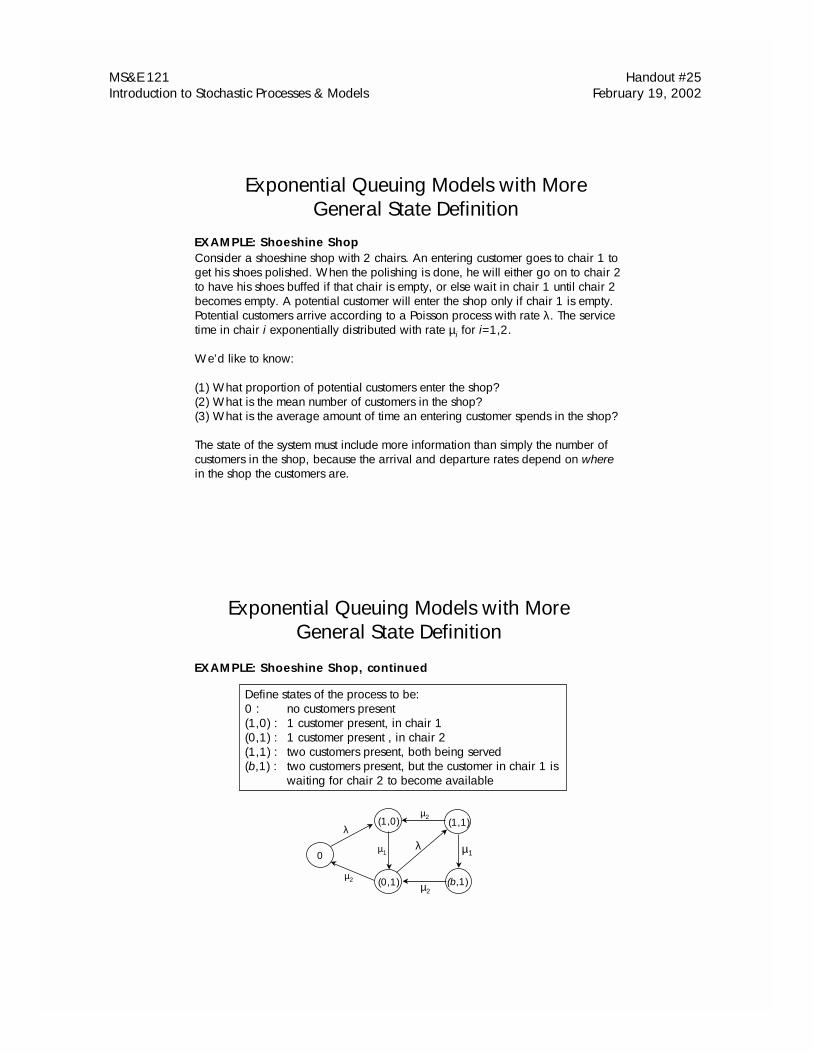
Define states of the process to be:0 : no customers present(1,0) : 1 customer present, in chair 1(0,1) : 1 customer present , in chair 2(1,1) : two customers present, both being served(b,1) : two customers present, but the customer in chair 1 is

waiting for chair 2 to become available

λ

….

(1,1)

µ1

(b,1)

0

λ

(0,1)

(1,0)

µ2

µ1

µ2

µ2




Q

b

=

−−

− +− +

−

�

�

��

�

�

��

0

1 0

0 1

1 1

1

1 1

2 2

2 1 2 1

2 2

( , )

( , )

( , )

( , )

( )

( )

λ λµ µ

µ λ µ λµ µ µ µ

µ µ

0

0

0

0

0

0 2 0 1

1 1 0 2 1 1

1 1 0 2 0 1 2 1

0 1 1 2 1 1

1 1 1 2 1

= − += − += − + += − += −

λ µλ µ µµ λ µ µλ µ µµ µ

P P

P P P

P P P

P P

P P

b

b

( , )

( , ) ( , )

( , ) ( , ) ( , )

( , ) ( , )

( , ) ( , )

( )

( )

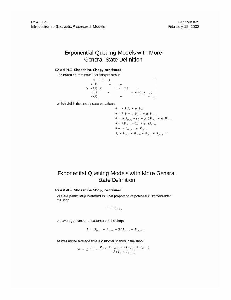
The transition rate matrix for this process is

which yields the steady state equations.

P P P P P b0 0 1 1 0 1 1 1 1+ + + + =( , ) ( , ) ( , ) ( , )


L P P P P b= + + +( , ) ( , ) ( , ) ( , )( )0 1 1 0 1 1 12

We are particularly interested in what proportion of potential customers enter the shop:

the average number of customers in the shop:

as well as the average time a customer spends in the shop:


P P0 0 1+ ( , )

W LP P P P

P Pb= =

+ + ++

/( )

( )( , ) ( , ) ( , ) ( , )

( , )

λ λ0 1 1 0 1 1 1

0 0 1

2




P P

P P P

P P P

P P

P P

b

b

0 0 1

1 0 0 1 1

0 1 1 0 1

0 1 1 1

1 1 1

2

2

3 2

3

2

== +

= +==

( , )

( , ) ( , )

( , ) ( , ) ( , )

( , ) ( , )

( , ) ( , )

Let’s suppose that the arrival rate λ=1 customer per minute. Consider first the case that µ1=1 and µ2 =2, i.e., the server for chair 2 is twice as fast. In that case, the steady state equations are:

From the steady state distribution, we can answer our questions:

(1) the proportion of potential customers entering the shop =

(2) (3)

P P P P P b0 0 1 1 0 1 1 1 1+ + + + =( , ) ( , ) ( , ) ( , )

L = + =2 2

3 72

3

3 7

2 8

3 7( )

914

1837

3728

)( )1,0(0

==+

=PP

LWλ

P P

P P

P b

0 1 0

0 1 1 1

1

1 2

3 7

1 6

3 76

3 7

2

3 71

3 7

= =

= =

=

,

,

( , )

( , ) ( , )

( , )

Solution:

P P0 0 1

1 8

3 7+ =( , )


EXAMPLE: Shoeshine Shop, continuedNow suppose that µ1=2 and µ2 =1, i.e., the server for chair 1 is twice as fast. In that case, the steady state equations are:

(1) the proportion of potential customers entering the shop =

(2) (3)

Having the server for the second chair server be faster leads to loss of more potentialcustomers, but shorter average waits and fewer customers in the shop on average.

P P

P P P

P P P

P P

P P

b

b

0 0 1

1 0 0 1 1

0 1 1 0 1

0 1 1 1

1 1 1

2

2 2

3

2

== += +

==

( , )

( , ) ( , )

( , ) ( , ) ( , )

( , ) ( , )

( , ) ( , )

P P P P P b0 0 1 1 0 1 1 1 1+ + + + =( , ) ( , ) ( , ) ( , )

L = + =5

1 12

3

1 11( ) W

L

P P=

+= =

λ ( )( , )0 0 1

11 1

6

1 1

6

Solution:

P P

P P

P b

0 1 0

0 1 1 1

1

3

1 1

2

1 13

1 1

1

1 12

1 1

= =

= =

=

,

,

( , )

( , ) ( , )

( , )

P P0 0 1

6

1 1+ =( , )


Networks of Markovian Queues

Queueing systems often provide more than a single service. Many real-world systems involve customers receiving a number of different services, each at a different service station, where each station has a queue for service. We can model systems of this kind using networks of queues. There are two types of queueing networks: open and closed. An open queueing network is one in which customers can enter and leave the system. A closed queueing network is one in which there are a fixed number of customers that never leave; new customers never enter.

We will be concerned with networks of Markovian queues called Jackson networks. These networks have exponentially distributed service times ateach service station and exponentially distributed interarrival times of new customers. The sequence of stations visited is governed by a probability matrix. We’ll consider first open and then closed Jackson networks. We’ll start off with an important result that will help with the analysis.

The Equivalence Property

Poisson arrivals

with rate λ

Poisson departures with rate λ

S servers, each with service times

~exp(µ)

In an M/M/S queue which is positive recurrent (i.e., λ < Sµ), the steady state output of the system is a Poisson process with the same rate as the input process. Note: S may be infinite.

The Equivalence Property


….wash

(1 server)µ1=60/hr

….wax

(1 server) µ2=45/hr

λ=30/hr

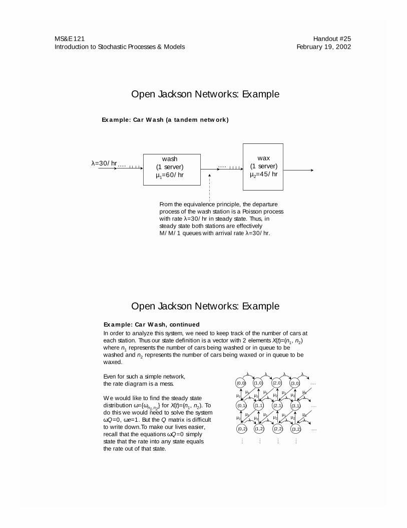
Example: Car Wash (a tandem network)

From the equivalence principle, the departure process of the wash station is a Poisson process with rate λ=30/hr in steady state. Thus, in steady state both stations are effectively M/M/1 queues with arrival rate λ=30/hr.

Open Jackson Networks: Example

Example: Car Wash, continuedIn order to analyze this system, we need to keep track of the number of cars ateach station. Thus our state definition is a vector with 2 elements X(t)=(n1, n2) where n1 represents the number of cars being washed or in queue to be washed and n2 represents the number of cars being waxed or in queue to be waxed.

Even for such a simple network,the rate diagram is a mess.

We would like to find the steady state distribution ω={ωn1,n2

} for X(t)=(n1, n2). To do this we would need to solve the systemωQ=0, ωe=1. But the Q matrix is difficult to write down.To make our lives easier, recall that the equations ωQ=0 simply state that the rate into any state equals the rate out of that state.

….

λ λ

(0,0)

λ λ

(1,0) (2,0) (3,0)

….(0,1) (1,1) (2,1) (3,1)

….(0,2) (1,2) (2,2) (3,2)

λ λλ λµ1 µ1 µ1 µ1µ2µ2 µ2


….

….

….

….

µ2

µ2




Example: Car Wash, continued

The equations ωQ=0 are given by

state rate out = rate in(0,0) λω0,0 = µ2ω0,1 (n1,0); n1>0 (λ + µ1)ωn1,0 = µ2ωn1,1 + λωn1-1,0 (0,n2); n2>0 (λ + µ2)ω0,n2

= µ2ω0,n2+1 + µ1ω1,n2-1 (n1,n2); n1,n2>0 (λ + µ1 + µ2)ωn1,n2

= µ2ωn1,n2+1 + µ1ωn1+1,n2-1 + λωn1-1,n2

To compute the steady state probabilities Pn1,n2

= ωn1,n2we must solve the above

equations along with

….

λ λ

(0,0)

λ λ

(1,0) (2,0) (3,0)

….(0,1) (1,1) (2,1) (3,1)

….(0,2) (1,2) (2,2) (3,2)



….

….

….

….

µ2

µ2

Pn nnn

n nnn

1 2

21

1 2

2100 00

1, ,=

∞

=

∞

=

∞

=

∞

�� = =ω


Example: Car Wash, continuedRather than solve the steady state equations directly, let’s guess at a solution.First, by the equivalence principal, we know station i is an M/M/1 queue with arrival rate λ and service rate µi. Assuming ρi = λ/µi <1 for i=1,2, we know

( )P n

n

n( )11 1

1 1

1

11 1at w ash s ta tio n =�

��

�

�� −

�

��

�

�� = −

λµ

λµ ρ ρ

P n

n

n( ) ( )22 2

2 2

2

21 1a t w a x s ta tio n =�

��

�

�� −

�

��

�

�� = −

λµ

λµ

ρ ρ

Now, if it were true that the number of cars at the wash and wax stations atany time were independent random variables, then we would know that

P P n n

P n P n

n n

n n

1 2

1 2

1 2

1 2 1 1 2 21 1

, ( )

( ( ) ( ) ( )

=

= = − −

at wash station and at wax station

at wash station) at wax station ρ ρ ρ ρ


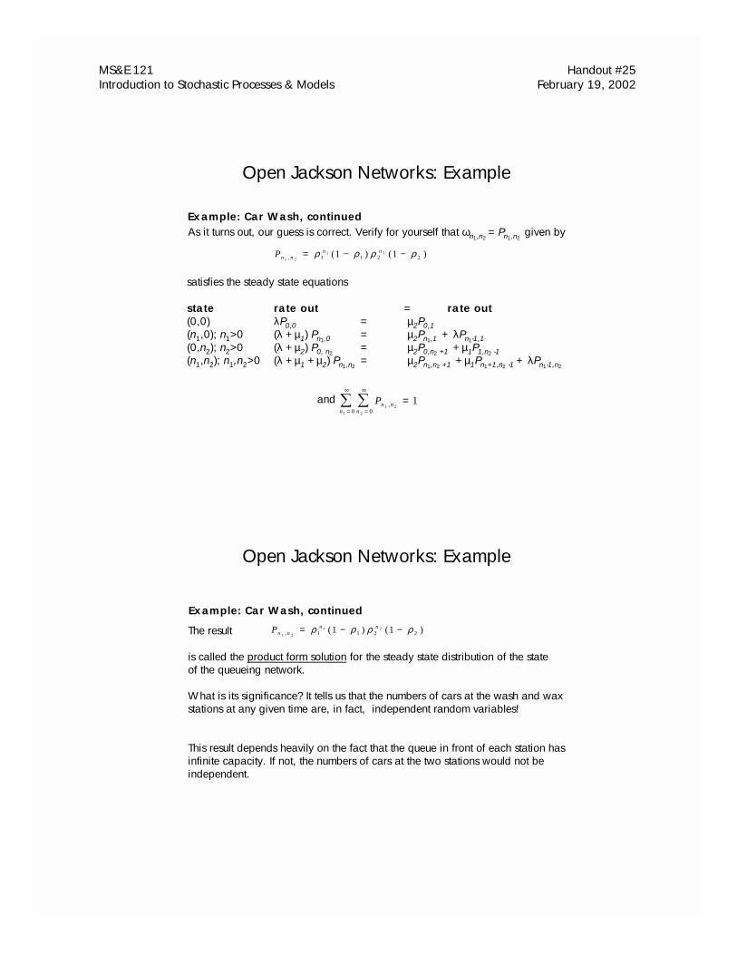
Example: Car Wash, continuedAs it turns out, our guess is correct. Verify for yourself that ωn1,n2

= Pn1,n2given by

Pn nn n

1 2

1 21 1 2 21 1, ( ) ( )= − −ρ ρ ρ ρ

satisfies the steady state equations

state rate out = rate out(0,0) λP0,0 = µ2P0,1 (n1,0); n1>0 (λ + µ1) Pn1,0 = µ2Pn1,1 + λPn1-1,1 (0,n2); n2>0 (λ + µ2) P0, n2

= µ2P0,n2 +1 + µ1P1,n2 -1 (n1,n2); n1,n2>0 (λ + µ1 + µ2) Pn1,n2

= µ2Pn1,n2 +1 + µ1Pn1+1,n2 -1 + λPn1-1,n2

and


Pn nnn

1 2

21 00

1,=

∞

=

∞

�� =


The result

is called the product form solution for the steady state distribution of the state of the queueing network.

What is its significance? It tells us that the numbers of cars at the wash and wax stations at any given time are, in fact, independent random variables!

This result depends heavily on the fact that the queue in front of each station hasinfinite capacity. If not, the numbers of cars at the two stations would not be independent.


Pn nn n

1 2

1 21 1 2 21 1, ( ) ( )= − −ρ ρ ρ ρ


Example: Car Wash, continuedThe product form solution of the the steady state distribution makes it easy to calculate the expected number of cars in the system:

L n n P n nnn

n nnn

n n= + = + − −=

∞

=

∞

=

∞

=

∞

�� ( ) ( ) ( ) ( ),1 200

1 200

1 1 2 221

1 2

21

1 21 1ρ ρ ρ ρ

= − − + − −=

∞

=

∞

=

∞

=

∞

� � � �n nn

n

n

n

n

n

n

n1 1 1

02 2

02 2 2

01 1

0

1

1

2

2

2

2

1

1

1 1 1 1ρ ρ ρ ρ ρ ρ ρ ρ( ) ( ) ( ) ( )

= −−

+ −−

=−

+−

=−

+−

= + =

( )( )

( )( )

11

11

1 1

3 0

3 0

3 0

1 53

11

12 2

2

22

1

1

2

2

1 2

ρρ

ρρ

ρρ

ρρ

ρρ

λµ λ

λµ λ

Notice that this equals the sum of the expected numbers of cars at the two stations, respectively.


= − + −=

∞

=

∞

� �n nn

n

n

n1 1 1

02 2 2

0

1

1

2

2

1 1ρ ρ ρ ρ( ) ( )


Using this last result and Little’s Law, we can compute the average time a carspends at the car wash:

WL L

= = =−

+−

= + =

λ λ µ λ µ λ1 1

1

3 0

1

1 5

1

1 0

1 2

h o u r = 6 m i n

Notice that this equals the sum of the average time a carspends at each of the two stations, respectively.

What made the computation of L and W easy in this example was the productform solution of the steady state distribution. It turns out that there is a much moregeneral framework under which a product form solutions are available. These arecalled Jackson networks.



Open Jackson Networks

An Open Jackson Network is a network of m service stations, where station i has

(1) an infinite queue

(2) customers arriving from outside the system according to a Poisson process with rate ai

(3) si identical servers, each with an exponential service time distribution with rate µi

(4) the probability that a customer exiting station i goes to station j is pij

(5) a customer exiting station i departs the system with probability 11

−=� pijj

m


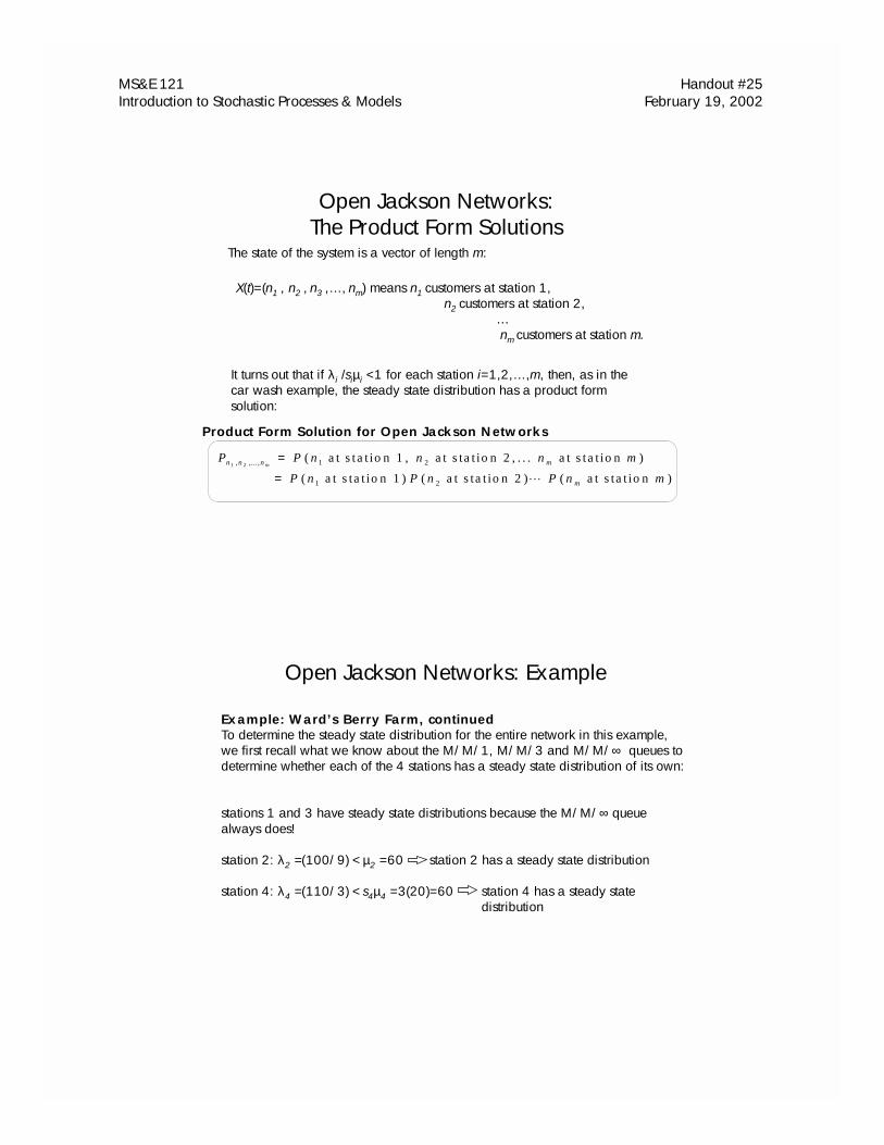
2: Berry Weighing Station1 server

4: Cashiers3 servers

….

….

Example: Ward’s Berry Farm

3: Farmstand(self-service)

1: Strawberry Field(self-service)

a1 =10/hr

a3 =30/hrµ3 =6/hr

µ2 =60/hr

µ1 =2/hr

µ4 =20/hr

p24 =0.6

p21=0.1

p23 =0.3

p34 =0.9

0.1

Recall from homework: self-service is effectively equivalent to having infinitely many servers.

p12=1


Open Jackson Networks: Traffic Equations

Traffic Equations for Open Jackson Networks

Define:

λ i = total arrival rate to station i (including external and internal arrivals)

The values {λ i, i=1,2…,m} must satisfy the following equations:

λ λi i j jij

m

a p i m= + ==�

1

1 2for , , . . . ,

total arrival rate into station i

external arrival rate into station i

total arrival rate from other stations

λ λi i j jij

m

a p i m= + ==�

1

1 2fo r , , . . . ,

Open Jackson Networks: ExampleExample: Ward’s Berry Farm, continuedIn this example, our traffic equations look like:

Solving these simultaneously gives us:

λ λ λ

λ λ λ

λ λ λ

λ λ λ λ

1 1 11

2

2 2 21

1

3 3 31

2

4 4 41

2 3

1 0 0 1

3 0 0 3

0 6 0 9

= + = +

= + =

= + = +

= + = +

=

=

=

=

�

�

�

�

a p

a p

a p

a p

j jj

m

j jj

m

j jj

m

j jj

m

( . )

( . )

( . ) ( . )

λ λ

λ

λ

1 2

3

4

1 0 0

9

3 03

1 0

1 0 0

9

1 0 0

36

1 0

1 0 0

9

9

1 0

1 0 0

3

1 1 0

3

= =

= + =

= + =


Open Jackson Networks: The Product Form Solutions

The state of the system is a vector of length m:

X(t)=(n1 , n2 , n3 ,…, nm) means n1 customers at station 1,n2 customers at station 2,

…nm customers at station m.

It turns out that if λ i /siµi <1 for each station i=1,2,…,m, then, as in the car wash example, the steady state distribution has a product form solution:

P P n n n m

P n P n P n m

n n n m

m

m1 2 1 2

1 2

, ,... , ( )

( ( ) ( )

=

=

a t s t a t io n 1 , a t s ta t io n 2 , . . . a t s t a t io n

a t s ta t io n 1 ) a t s ta t io n 2 a t s ta t io n�

Product Form Solution for Open Jackson Networks

Example: Ward’s Berry Farm, continuedTo determine the steady state distribution for the entire network in this example, we first recall what we know about the M/M/1, M/M/3 and M/M/∞ queues to determine whether each of the 4 stations has a steady state distribution of its own:

stations 1 and 3 have steady state distributions because the M/M/∞ queuealways does!

station 2: λ2 =(100/9) < µ2 =60 station 2 has a steady state distribution

station 4: λ4 =(110/3) < s4µ4 =3(20)=60 station 4 has a steady state distribution



Example: Ward’s Berry Farm, continuedWe compute each station’s own steady state distribution using what we already know about the M/M/1, M/M/3 and M/M/∞ queues:

P jj

ej

(( )

!a t s t a t i o n 1 ) = −λ µ λ µ1 1 1 1

P j j( ( ) ( )a t s t a t i o n 2 ) = −1 2 2 2 2λ µ λ µ

P j jK j

K j

j

j

j

(

( )

!( )

( )

!( )

a t s t a t i o n 4 )f o r

f o r

=+ ≤ ≤

+ ≥

�

��

��

−

−−

λ µ

λ µ

4 4 1

4 43

1

1 0 3

3 31 4

w h e r e Ki

i

i

= +−

�

��

�

��

=�

( )

!

( )

! ( )

λ µ λ µλ µ

4 4

0

24 4

3

4 43

1

1 3

P jj

ej

(( )

!a t s t a t i o n 3 ) = −λ µ λ µ3 3 3 3


Example: Ward’s Berry Farm, continuedWe express the steady state distribution of the entire network in product form:

P

P n P n P n P n

n n n n1 2 3 4

1 2 3 43 4

, , ,

( ( ) ( ) ( )= a t s ta tio n 1 ) a t s ta tio n 2 a t s ta tio n a t s ta tio n

= ⋅ −

⋅ ⋅+ ≤ ≤

+ ≥

�

��

��

−

−

−

−−

( )

!( ) ( )

( )

!

( )

!( )

( )

!( )

λ µλ µ λ µ

λ µλ µ

λ µ

λ µ

λ µ

1 1

12 2 2 2

3 3

3

4 4

4

14

4 43

14

1

1 1 2

3

3 3

4

4

4

1

1 0 3

3 31 4

nn

n

n

n

n

ne

ne

nK n

K n

i f

if

6

1556.5556.5

122

104962.1

)11.71()185.01(

)1()1( 3311

−

−−−

−−−

×=

+−=

+−=

ee

Kee µλµλ µλP0 0 0 0, , ,

This looks cumbersome but is easily evaluated for any particular state vector (n1, n2, n3, n4). An example is (n1, n2, n3, n4) = (0,0,0,0):



Open Jackson NetworksSteps to Analyze an Open Jackson Network

(1) Solve the traffic equations

(2) Check that λ i < si µi for each station i=1,…,m. If NO, the number of customers in the network blows up,

so there is no steady state distribution. If YES, go to step 3.

(3) For each station i, calculate the steady state distribution for an M/M/si queue with arrival rate λ i and the service rate µi.

(4) The steady state probability that there are n1 customers at station 1, n2 customers at station 2,…., nm customers at station m is just

ω ω ω ωi i i i= ( , , , . . . )0 1 2

P P n P n P nn n n m

n n nm

m

m

1 2

1 2

1 2

1 2

, ,..., ( ) ( ) ( )=

= ⋅ ⋅

a t s ta t io n 1 a t s ta t io n 2 a t s ta t io n m�

�ω ω ω

λ λi i j jij

m

a p i m= + ==�

1

1 2fo r , , . . . ,

Open Jackson NetworksIn the special case that all n stations have a single server (si=1 for all i) then the analysis is particularly easy:


(2) Check that ρi = λ i/µi <1 for each station i=1,…,m. If NO, there is no steady state distribution. If YES, go to step 3.

(3) For each station i, the steady state distribution for an M/M/1 queue with arrival rate λ i and the service rate µi is:


ω ω ω ωi i i i= ( , , , . . . )0 1 2

Pn n n n n nm n n

m mn

ii

m

in

m m

m

i

1 2 1 2

1 21 21 1 2 2

1

1 1 1

1

, ,... , ( ) ( ) ( ) ( ) ( ) ( )

( ) ( )

= ⋅ = − − −

= −=

∏

ω ω ω ρ ρ ρ ρ ρ ρ

ρ ρ

� �

ω ρ ρji

i ij= −( )( )1

λ λi i j jij

m

a p i m= + ==�

1

1 2fo r , , . . . ,


Example: Ward’s Berry Farm, continuedWard’s Berry Farm makes, on average, $15 per hour that a single customer spends picking berries. What is their average hourly income from the berry field? It’s

where

Thus, their average hourly income from the berry field alone is $83.40.

115$ L


56.52

100/9

1

11 ===

µλ

L

Example: Ward’s Berry Farm, continuedWhat is the average number of people at Ward’s Berry Farm at a given point in time in steady state? By the product form solution for Open Jackson Networks, we know the answer is

where Li is the average number of people at station i in steady state.

4321 LLLLL +++=


20.)1(!3

)()1(

56.56

100/3

28.))9/100(-60(

9/100

)-(

56.52

100/9

24

43

44144

3

33

22

22

1

11

=−

+=

===

===

===

−

ρρµλ

µλ

λµλ

µλ

KL

L

L

L

4

4

4

44 3 µ

λµ

λρ ==S

where

6.114321 =+++= LLLLL

is the average steady state number of people at the farm.


Example: Ward’s Berry Farm, continuedWhat is the average duration time a visiting customer spends at the farm?It turns out we can’t just add average times they spend at each station, because the customer doesn’t necessarily visit each station exactly once. Instead, we can just use Little’s Law:

where λ represents the average total external arrival rate to the entire system, i.e.,

So a visiting customer spends, on average,

hours at the farm.

WL λ=


4030104321 =+=+++= aaaaλ

29.40/6.11/ === λLW

Closed Jackson Networks

A closed Jackson network of queues is a network with a fixed number n of customers and m service stations, where station i has

(1) an infinite queue

(2) si identical servers, each with an exponential service time distribution with rate µi

(3) the probability that a customer exiting station i goes to station j is pij

(4) no customers exiting the system, i.e.,

(5) no arrivals of customers from outside the system

p ijj

m

=� =1

1



Traffic Equations for Closed Jackson Networks

As in the open network case, we let

λ i = total arrival rate to station i

where this time there are no external arrivals.

Now the values {λ i, i=1,2…,m} must satisfy:

λ λ

λ

i j jij

m

ii

m

p i m= =

=

=

=

�

�

1

1

1 2

1

for , , . . . ,

Closed Jackson NetworksSteps to Analyze a Closed Jackson Network


If a solution exists, go to step 2. If not, there is no steady state distribution.

(2) For each station i, calculate the steady state distribution for an M/M/si queue with arrival rate λ i and the service rate µi.(If λ i exceeds µi, and si=1, then it’s okay to use the steady state distribution anyway.)

ω ω ω ωi i i i= ( , , , . . . )0 1 2

λ λ λi j jij

m

ii

m

p i m= = == =� �

1 1

1 2 1for , , . . . , ,

continued….



P

n n n n

n n n nn n n

m

n n nm

j j jm

j j jj j j n

mm

m

m

m

m

1 2

1 2

1 2

1 2

1 2

0 1 21 2

1 2

0

1 2, ,...,

, ,...,...

. .

. .=

+ + ≠⋅

⋅+ + =

�

�

��

�

��

≥+ + + =

�

i f .

i f .ω ω ω

ω ω ω�

�


Steps to Analyze a Closed Jackson Network

Closed Jackson Networks: Example

Example: Roommate NetworkSuppose that between yourself and your two roommates, you own 2 Gameboys. When you get your hands on one, you tend to use it for a time that’s exponentially distributed with mean of 1 hour. When you’re tired of it, you give it to your roommate Barbara with with probability 0.8 or your other roommate Joyce with probability 0.2. The lengths of time that Barbara and Joyce keep a Gameboy is exponentially distributed with mean of 1.5 hours and 2 hours, respectively. Barbara will always give the one she’s been playing with to you when she’s through, whereas Joyce give it to you only 60% of the time; the rest of the time she’ll let Barbara have it next. What’s the probability that each of your roommates has Gameboy, but you don’t?

You(µ1=1)

1

Barbara(µ2=2/3)

2Joyce

(µ3=1/2)

3

p12=0.8 p13=0.2

p21=1 p31=.6

p32=.4



Example: Roommate network, continued(1) First we solve the traffic equations to obtain the arrival rates are each “station”:

The resulting arrival rates are:

λ λ λi j jij

m

ii

m

p i m= = == =� �

1 1

1 2 1for , , . . . , ,

λ λ λλ λ λλ λλ λ λ

1 2 3

2 1 3

3 1

1 2 3

0 6

0 8 0 4

0 2

1

= += +=+ + =

( . )

( . ) ( . )

( . )

You(µ1=1)

1

Barbara(µ2=2/3)

2Joyce

(µ3=1/2)

3

p12=0.8 p13=0.2

p21=1 p31=.6

p32=.4

λ λ λ1 2 3

2 5

5 2

2 2

5 2

5

5 2= = =, ,


(2) We now calculate the steady state distribution for each station i by modeling it as an M/M/1 queue with arrival rate λ i and the service rate µi.

station 1 (you):

station 2 (Barbara):

station 3 (Joyce):

(3) Now we want to compute the steady state probability that each of your roommates has a Gameboy. This probability is denoted by

Example: Roommate network, continued

ω j

j

1 2 7

5 2

2 5

5 2= �

��

��

��

ω j

j

2 1 9

5 2

3 3

5 2= �

��

��

��

ω j

j

3 4 2

5 2

1 0

5 2= �

��

��

��

P0 1 1, ,



P

n n n

n n nn n n

n n n

j j jj j jj j j

1 2 3

1 2 3

1 2 3

1 2 31 2 3

0 2

2

1 2 31 2 3

1 2 3

02

1 2 3, ,

, ,

=

+ + ≠⋅ ⋅

⋅ ⋅+ + =

�

�

��

�

��

≥+ + =

�

i f

i fω ω ω

ω ω ω

The steady state probability that there are n1 Gameboys with you, n2 Gameboys with Barbara, and n3 Gameboys with Joyce is

Let’s first compute the denominator:


ω ω ωj j jj j jj j j

1 2 3

1 2 31 2 3

1 2 3

02

⋅ ⋅≥

+ + =

�, ,


j j j j j j1 2 3 1 2 30 2, , ,≥ + + =There are six feasible combinations of indices (j1, j2, j3) that appear in the sum, namely those satisfying

(j1, j2, j3)

(2, 0, 0)

(0, 2, 0)

(0, 0, 2)

(1, 1, 0)

(1, 0, 1)

(0, 1, 1)


ω ω ωj j j1 2 3

1 2 3⋅ ⋅

ω ω ω21

02

03

22 75 2

2 55 2

1 95 2

4 25 2

= ��

��

��

��

��

��

ω j

j

2 1 9

5 2

3 3

5 2= �

��

��

��

ω j

j

3 4 2

5 2

1 0

5 2= �

��

��

��

ω ω ω01

22

03

22 75 2

1 95 2

3 35 2

4 25 2

= ��

��

��

��

��

��

ω ω ω01

02

23

22 7

5 2

1 9

5 2

4 2

5 2

1 0

5 2= �

��

��

��

��

��

ω ω ω11

12

03 2 7

5 2

2 5

5 2

1 9

5 2

3 3

5 2

4 2

5 2= �

��

��

��

��

��

��

ω ω ω11

02

13 2 7

5 2

2 5

5 2

1 9

5 2

4 2

5 2

1 0

5 2= �

��

��

��

��

��

��

ω ω ω01

12

13 2 7

5 2

1 9

5 2

3 3

5 2

4 2

5 2

1 0

5 2= �

��

��

��

��

��

��

ω j

j

1 2 7

5 2

2 5

5 2= �

��

��

��

we’re using:


Closed Jackson Networks: ExampleExample: Roommate network, continued

ω ω ωj j jj j jj j j

1 2 3

1 2 31 2 3

1 2 3

02

⋅ ⋅≥

+ + =

�, ,

ω ω ω21

02

03

22 75 2

2 55 2

1 95 2

4 25 2

= ��

��

��

��

��

��

ω ω ω01

22

03

22 75 2

1 95 2

3 35 2

4 25 2

= ��

��

��

��

��

��

ω ω ω01

02

23

22 7

5 2

1 9

5 2

4 2

5 2

1 0

5 2= �

��

��

��

��

��

ω ω ω11

12

03 2 7

5 2

2 5

5 2

1 9

5 2

3 3

5 2

4 2

5 2= �

��

��

��

��

��

��

ω ω ω11

02

13 2 7

5 2

2 5

5 2

1 9

5 2

4 2

5 2

1 0

5 2= �

��

��

��

��

��

��

ω ω ω01

12

13 2 7

5 2

1 9

5 2

3 3

5 2

4 2

5 2

1 0

5 2= �

��

��

��

��

��

��

=

+

+

+

+

+

= 0.1824

P

n n n

n n nn n n

n n n

j j jj j jj j j

1 2 3

1 2 3

1 2 3

1 2 31 2 3

0 2

2

1 2 31 2 3

1 2 3

02

1 2 3, ,

, ,

=

+ + ≠⋅ ⋅

⋅ ⋅+ + =

�

�

��

�

��

≥+ + =

�

i f

i fω ω ω

ω ω ω



Pj j j

j j jj j j

0 1 101

12

13

1 2 3

02

1 2 3

1 2 3

1 2 3

0 0 1 8 7

0 1 8 2 40 1 0 2 5, ,

, ,

.

..=

⋅ ⋅⋅ ⋅

= =

≥+ + =

�

ω ω ωω ω ω

The probability that each of your roommates has a Gameboy and you don’t is


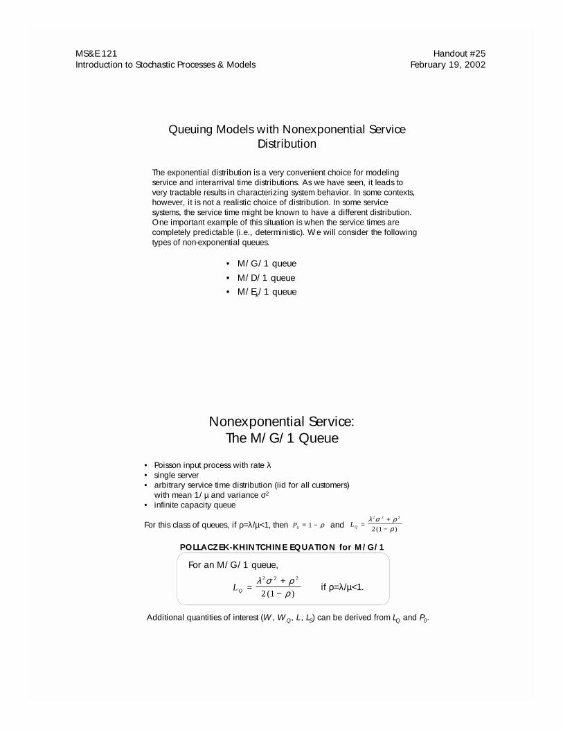
Queuing Models with Nonexponential Service Distribution

• M/G/1 queue• M/D/1 queue• M/Ek/1 queue

The exponential distribution is a very convenient choice for modeling service and interarrival time distributions. As we have seen, it leads to very tractable results in characterizing system behavior. In some contexts, however, it is not a realistic choice of distribution. In some service systems, the service time might be known to have a different distribution. One important example of this situation is when the service times are completely predictable (i.e., deterministic). We will consider the following types of non-exponential queues.

Nonexponential Service:The M/G/1 Queue

• Poisson input process with rate λ• single server• arbitrary service time distribution (iid for all customers)

with mean 1/µ and variance σ2

• infinite capacity queue

For this class of queues, if ρ=λ/µ<1, then and

LQ =+

−λ σ ρ

ρ

2 2 2

2 1( )

For an M/G/1 queue,

if ρ=λ/µ<1.

POLLACZEK-KHINTCHINE EQUATION for M/G/1

LQ =+

−λ σ ρ

ρ

2 2 2

2 1( )P0 1= − ρ

Additional quantities of interest (W, WQ, L , LS) can be derived from LQ and P0.


The M/G/1 Queue: Example

Suppose that customers arrive at the McDonald’s drive-thru at a rate of 30 per hour. The time to until any given car completes service is uniformly distributed on the interval [0,3] minutes.

(1) What is the average amount of time a car spends waiting to be served? (2) What is the average number of cars being served or waiting to be served?

The mean service time is 1.5 minute (obtained by taking the mean of a uniform [0,3] random variable) so the average service rate µ is 2/3 cars/minute. Thus ρ=λ/µ=3/4. The variance of the service time is σ2 = (3)2/12 = 3/4. The average waiting time in queue for each car, measured in minutes, is computed using the P-K equation and our useful relationship between LQ and WQ :

EXAMPLE: McD’s Drive Thru

WL L

Q

Q Q= = =+−

=+

=λ λ

λ σ ρλ ρ

2 2 2 2 2

2 1

0 5 0 7 5 0 7 5

2 0 5 0 2 53

( )

( . ) ( . ) ( . )

( . )( . )m in u te s

The M/G/1 Queue: Example

The average number of cars being served or waiting to be served is

L = LQ + LS

Since LS = (1-P0) = ρ for an M/G/1 queue, L equals

EXAMPLE: McD’s Drive Thru

L L LQ S= + =+

−+

=+

+ =

λ σ ρρ

ρ2 2 2

2 2

2 1

0 5 0 7 5 0 7 5

2 0 2 50 7 5 2 2 5

( )

( . ) ( . ) ( . )

( . )( . ) . c a rs


Nonexponential Service:The M/D/1 Queue

• Poisson input process with rate λ• single server• service time is deterministic and equal to 1/µ • infinite capacity queue

LQ =−

ρρ

2

2 1( )

For an M/D/1 queue,

where ρ=λ/µ

POLLACZEK-KHINTCHINE EQUATION for M/D/1

L Q =−

ρρ

2

2 1( )

P0 1= − ρThis is a special case of the M/G/1 queue in which σ2=0. As in the general case,if ρ=λ/µ<1, then . Moreover, in this case the P-K equation reduces to

The M/D/1 Queue: Example

Let’s compare two different employees at the drive thru window. Ann’s service time is uniformly distributed on the interval [0,3] minutes. Jim is slower on average, but more consistent: he completes service for every car in exactly 1.55 minutes every time. Which server makes customers wait less time from entry in the queue until completing service?

We’ve already seen that Ann’s service performance leads to:

so

EXAMPLE: McD’s Drive Thru, again

W W WQ S= + = + =3 1 5 4 5. . m in u te s

WL L

Q

Q Q= = =+−

=+

=λ λ

λ σ ρλ ρ

2 2 2 2 2

2 1

0 5 0 7 5 0 7 5

2 0 5 0 2 53

( )

( . ) ( . ) ( . )

( . ) ( . )m in u te s


The M/D/1 Queue: Example

Since Jim’s service time is deterministic, the variance of his service time is zero. In his case, ρ=λ/µ=0.775. By contrast, Jim has people wait in queue on average

Although Ann’s average service time is faster, Jim’s consistency leads to shorter waits.

EXAMPLE: McD’s Drive Thru, continued

W W WQ S= + = + =2 6 6 9 4 1 5 5 4 2 1 9 4. . . m in u t e s

WL L

Q

Q Q= = =−

= =λ λ

ρλ ρ

2 2

2 1

7 7 5

2 0 5 2 2 52 6 6 9 4

( )

( . )

( . ) ( . ). m in u te s

Nonexponential Service:The M/Ek/1 Queue

Now we consider another special case of the M/G/1 queue, namely the M/ Ek/1 queue. The notation Ek stands for the Erlang distribution with shape parameter k. To motivate this type of queue, we first mention some importantfacts about the Erlang distribution.

A random variable X having an Erlang distribution with parameters (µ, k) has probability density function

and mean and variance E X( ) =1

µ

f xk x e

kx

k k k x

( )( )

( ) !=

−≥

− −µ µ1

10f o r

V a r ( )Xk

=1

2µ

The Erlang (µ,k) random variable is also called a Gamma (k,µk) random variable.

Note: if k = 1, then X is exponentially distributed with parameter µ

The Erlang Distribution


The Erlang Distribution

Let be independent and identically distributed exponential random variables with parameter nµ. Then the random variable

has an Erlang distribution with parameters (µ, n).

Y Y Yn1 2, , . . . ,

Y Y Y Yn= + + +1 2 . . .

Useful Fact About the Erlang Distribution

The Erlang distribution is of particular significance in queueing theory because of this useful fact. To see why, imagine a queuing system where the server (or servers) performs not just a single task that takes an exponential length of time but instead a sequence of n tasks, where each task takes an exponential length of time. When each task’s time has parameter nµ (mean 1/nµ) then the length of time to complete all tasks has an Erlang distribution with parameters (µ, n).

Nonexponential Service:The M/Ek/1 Queue

• Poisson input process with rate λ • single server• Erlang (µ,k) service time distribution; mean 1/µ and variance 1/kµ2

• infinite capacity queue

As for the general M/G/1 case, if ρ=λ/µ<1, then . Applying the P-K equation to this case yields

For an M/Ek/1 queue,

if ρ=λ/µ<1.

POLLACZEK-KHINTCHINE EQUATION for M/Ek/1

Lk k

Q =+

−=

+−

λ µ ρρ

ρρ

2 2 2 2

2 1

1 1

2 1

/

( )

(( / ) )

( )

P0 1= − ρ

Lk

Q =+

−ρ

ρ

2 1 1

2 1

(( / ) )

( )


The M/Ek/1 Queue: Example

Students working on their EESOR 121 homework send email asking for help at a rate of 1 email per hour. When an email arrives I get right to work answering that person’s email if I am not busy answering another student’s email at the time. Each student’s email asks one question for each of the 7 problems on the homework.) The time each question takes me to answer is exponentially distributed with mean 3 minutes, so I am capable of replying to one email every 21 minutes on average.

(1) What is the average time a student waits for a reply?

(2) If I would like to spend only 10% of of my time answering homework questions, how many homework problems should I assign each week?

EXAMPLE: Homework Questions


It is given that the time to answer each question is exponentially distributed with parameter 3. Since there are n=7 questions one each homework set, letting 1/nµ=3 implies that the time it takes me to answer one entire email has an Erlangdistribution with parameters (µ, n)=(1/21,7).

In this example ρ=λ/µ = 7/20. The P-K equation tells us

We also know

(1) The average time a student waits for a reply is

EXAMPLE: Homework, continued

Ln

Q =+

−=

+=

ρρ

2 21 1

2 1

7 2 0 1 7 1

2 1 3 2 0

7

6 5

(( / ) )

( )

( / ) (( / ) )

( / )

L PS = − = =1 17

2 00( ) ρ

W L L LS Q= = + = +��

�� = �

��

��/ ( ) /λ λ 6 0

7

2 0

7

6 56 0

1 1 9

2 6 0

= 2 7 .4 6 m in u te s = 0 .4 5 7 7 h o u r s



(2) Let n be the number of questions on the homework. My rate of replying to emails is then µ = 1/3n per hour. If I would like to spend at most 10% of of my time answering homework questions, then I require

This holds only if

or

I should assign at most 2 problems per week.

EXAMPLE: Homework, continued

1 0 10− ≤P .

13

6 0 2 00 10− = = = = ≤P

n nρ

λµ .

n ≤ 2

Date post:	22-Feb-2019
Category:	Documents
Upload:	doandung
View:	221 times
Download:	0 times

Queuing Theory - unisi.it · MS&E 121 Handout #25 Introduction to Stochastic Processes & Models...

Documents