New York University, Microsoft Research New England andMassachusetts Institute of Technology
We study an admissions control problem, where a queue with servicerate 1 − p receives incoming jobs at rate λ ∈ (1 − p,1), and the decisionmaker is allowed to redirect away jobs up to a rate of p, with the objective ofminimizing the time-average queue length.
We show that the amount of information about the future has a sig-nificant impact on system performance, in the heavy-traffic regime. Whenthe future is unknown, the optimal average queue length diverges at rate∼ log1/(1−p)
11−λ
, as λ → 1. In sharp contrast, when all future arrival andservice times are revealed beforehand, the optimal average queue length con-verges to a finite constant, (1 − p)/p, as λ → 1. We further show that the fi-nite limit of (1 −p)/p can be achieved using only a finite lookahead windowstarting from the current time frame, whose length scales as O(log 1
1−λ), as
λ → 1. This leads to the conjecture of an interesting duality between queuingdelay and the amount of information about the future.
1. Introduction.
1.1. Variable, but predictable. The notion of queues has been used extensivelyas a powerful abstraction in studying dynamic resource allocation systems, whereone aims to match demands that arrive over time with available resources, and aqueue is used to store currently unprocessed demands. Two important ingredientsoften make the design and analysis of a queueing system difficult: the demandsand resources can be both variable and unpredictable. Variability refers to the factthat the arrivals of demands or the availability of resources can be highly volatileand nonuniformly distributed across the time horizon. Unpredictability means thatsuch nonuniformity “tomorrow” is unknown to the decision maker “today,” andshe is obliged to make allocation decisions only based on the state of the system atthe moment, and some statistical estimates of the future.
While the world will remain volatile as we know it, in many cases, the amountof unpredictability about the future may be reduced thanks to forecasting technolo-gies and the increasing accessibility of data. For instance:
Received January 2013; revised April 2013.1Supported in part by a research internship at Microsoft Research New England and by NSF Grants
CMMI-0856063 and CMMI-1234062.MSC2010 subject classifications. 60K25, 60K30, 68M20, 90B36.Key words and phrases. Future information, queuing theory, admissions control, resource pool-
ing, random walk, online, offline, heavy-traffic asymptotics.
(1) advance booking in the hotel and textile industries allows for accurate fore-casting of demands ahead of time [9];
(2) the availability of monitoring data enables traffic controllers to predict thetraffic pattern around potential bottlenecks [18];
(3) advance scheduling for elective surgeries could inform care providers sev-eral weeks before the intended appointment [12].
In all of these examples, future demands remain exogenous and variable, yet thedecision maker is revealed with (some of) their realizations.
Is there significant performance gain to be harnessed by “looking into the fu-ture?” In this paper we provide a largely affirmative answer, in the context of aclass of admissions control problems.
1.2. Admissions control viewed as resource allocation. We begin by infor-mally describing our problem. Consider a single queue equipped with a server thatruns at rate 1 − p jobs per unit time, where p is a fixed constant in (0,1), as de-picted in Figure 1. The queue receives a stream of incoming jobs, arriving at rateλ ∈ (0,1). If λ > 1 − p, the arrival rate is greater than the server’s processing rate,and some form of admissions control is necessary in order to keep the system sta-ble. In particular, upon its arrival to the system, a job will either be admitted to thequeue, or redirected. In the latter case, the job does not join the queue, and, fromthe perspective of the queue, disappears from the system entirely. The goal of thedecision maker is to minimize the average delay experienced by the admitted jobs,while obeying the constraint that the average rate at which jobs are redirected doesnot exceeded p.2
One can think of our problem as that of resource allocation, where a decisionmaker tries to match incoming demands with two types of processing resources:a slow local resource that corresponds to the server and a fast external resourcethat can process any job redirected to it almost instantaneously. Both types of re-sources are constrained, in the sense that their capacities (1 − p and p, resp.)cannot change over time, by physical or contractual predispositions. The process-ing time of a job at the fast resource is negligible compared to that at the slow
FIG. 1. An illustration of the admissions control problem, with a constraint on the a rate of redi-rection.
2Note that as λ → 1, the minimum rate of admitted jobs, λ − p, approaches the server’s capacity1 − p, and hence we will refer to the system’s behavior when λ → 1 as the heavy-traffic regime.
QUEUING WITH FUTURE INFORMATION 2093
resource, as long as the rate of redirection to the fast resource stays below p in thelong run. Under this interpretation, minimizing the average delay across all jobs isequivalent to minimizing the average delay across just the admitted jobs, since thejobs redirected to the fast resource can be thought of being processed immediatelyand experiencing no delay at all.
For a more concrete example, consider a web service company that enters along-term contract with an external cloud computing provider for a fixed amountof computation resources (e.g., virtual machine instance time) over the contract pe-riod.3 During the contract period, any incoming request can be either served by thein-house server (slow resource), or be redirected to the cloud (fast resource), andin the latter case, the job does not experience congestion delay since the scalabilityof cloud allows for multiple VM instance to be running in parallel (and potentiallyon different physical machines). The decision maker’s constraint is that the totalamount of redirected jobs to the cloud must stay below the amount prescribed bythe contract, which, in our case, translates into a maximum redirection rate overthe contract period. Similar scenarios can also arise in other domains, where theslow versus fast resources could, for instance, take on the forms of:
(1) an in-house manufacturing facility versus an external contractor;(2) a slow toll booth on the freeway versus a special lane that lets a car pass
without paying the toll;(3) hospital bed resources within a single department versus a cross-departmen-
tal central bed pool.
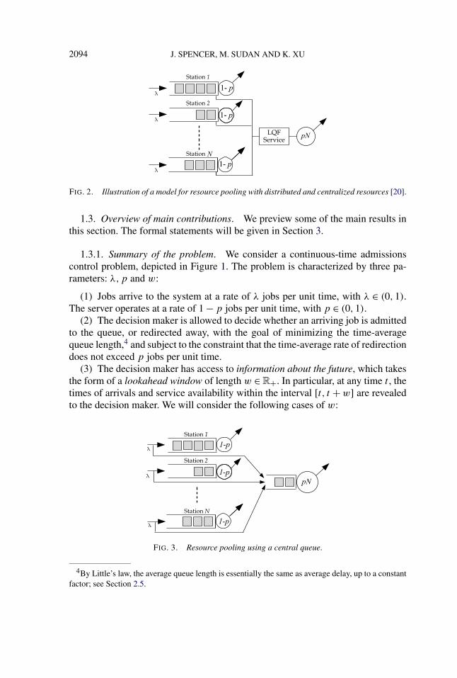
In a recent work [20], a mathematical model was proposed to study the benefitsof resource pooling in large scale queueing systems, which is also closely con-nected to our problem. They consider a multi-server system where a fraction 1 −p
of a total of N units of processing resources (e.g., CPUs) is distributed among aset of N local servers, each running at rate 1 − p, while the remaining fraction ofp is being allocated in a centralized fashion, in the form of a central server thatoperates at rate pN (Figure 2). It is not difficult to see, when N is large, the centralserver operates at a significantly faster speed than the local servers, so that a jobprocessed at the central server experiences little or no delay. In fact, the admis-sions control problem studied in this paper is essentially the problem faced by oneof the local servers, in the regime where N is large (Figure 3). This connection isexplored in greater detail in Appendix B, where we discuss what the implicationsof our results in context of resource pooling systems.
3Example. As of September 2012, Microsoft’s Windows Azure cloud services offer a 6-monthcontract for $71.99 per month, where the client is entitled for up to 750 hours of virtual machine(VM) instance time each month, and any additional usage would be charged at a 25% higher rate.Due to the large scale of the Azure data warehouses, the speed of any single VM instance can betreated as roughly constant and independent of the total number of instances that the client is runningconcurrently.
2094 J. SPENCER, M. SUDAN AND K. XU
FIG. 2. Illustration of a model for resource pooling with distributed and centralized resources [20].
1.3. Overview of main contributions. We preview some of the main results inthis section. The formal statements will be given in Section 3.
1.3.1. Summary of the problem. We consider a continuous-time admissionscontrol problem, depicted in Figure 1. The problem is characterized by three pa-rameters: λ,p and w:
(1) Jobs arrive to the system at a rate of λ jobs per unit time, with λ ∈ (0,1).The server operates at a rate of 1 − p jobs per unit time, with p ∈ (0,1).
(2) The decision maker is allowed to decide whether an arriving job is admittedto the queue, or redirected away, with the goal of minimizing the time-averagequeue length,4 and subject to the constraint that the time-average rate of redirectiondoes not exceed p jobs per unit time.
(3) The decision maker has access to information about the future, which takesthe form of a lookahead window of length w ∈ R+. In particular, at any time t , thetimes of arrivals and service availability within the interval [t, t + w] are revealedto the decision maker. We will consider the following cases of w:
FIG. 3. Resource pooling using a central queue.
4By Little’s law, the average queue length is essentially the same as average delay, up to a constantfactor; see Section 2.5.
QUEUING WITH FUTURE INFORMATION 2095
(a) w = 0, the online problem, where no future information is available.(b) w = ∞, the offline problem, where entire the future has been revealed.(c) 0 < w < ∞, where future is revealed only up to a finite lookahead window.
Throughout, we will fix p ∈ (0,1), and be primarily interested in the system’sbehavior in the heavy-traffic regime of λ → 1.
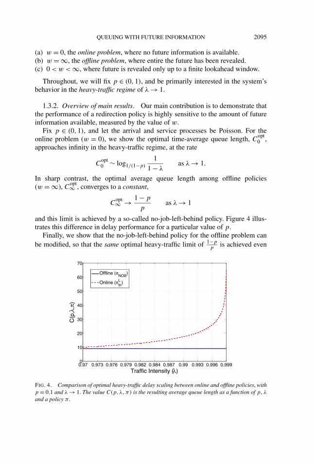
1.3.2. Overview of main results. Our main contribution is to demonstrate thatthe performance of a redirection policy is highly sensitive to the amount of futureinformation available, measured by the value of w.
Fix p ∈ (0,1), and let the arrival and service processes be Poisson. For theonline problem (w = 0), we show the optimal time-average queue length, C
opt0 ,
approaches infinity in the heavy-traffic regime, at the rate
Copt0 ∼ log1/(1−p)
1
1 − λas λ → 1.
In sharp contrast, the optimal average queue length among offline policies(w = ∞), C
opt∞ , converges to a constant,
Copt∞ → 1 − p
pas λ → 1
and this limit is achieved by a so-called no-job-left-behind policy. Figure 4 illus-trates this difference in delay performance for a particular value of p.
Finally, we show that the no-job-left-behind policy for the offline problem canbe modified, so that the same optimal heavy-traffic limit of 1−p
pis achieved even
FIG. 4. Comparison of optimal heavy-traffic delay scaling between online and offline policies, withp = 0.1 and λ → 1. The value C(p,λ,π) is the resulting average queue length as a function of p, λ
and a policy π .
2096 J. SPENCER, M. SUDAN AND K. XU
with a finite lookahead window, w(λ), where
w(λ) = O(
log1
1 − λ
)as λ → 1.
This is of practical importance because in any realistic application, only a finiteamount of future information can be obtained.
On the methodological end, we use a sample path-based framework to analyzethe performance of the offline and finite lookahead policies, borrowing tools fromrenewal theory and the theory of random walks. We believe that our techniquescould be substantially generalized to incorporate general arrival and service pro-cesses, diffusion approximations as well as observational noises. See Section 8 fora more elaborate discussion.
1.4. Related work. There is an extensive body of work devoted to variousMarkov (or online) admissions control problems; the reader is referred to thesurvey of [19] and references therein. Typically, the problem is formulated asan instance of a Markov decision problem (MDP), where the decision maker,by admitting or rejecting incoming jobs, seeks to maximize a long-term averageobjective consisting of rewards (e.g., throughput) minus costs (e.g., waiting timeexperienced by a customer). The case where the maximization is performed sub-ject to a constraint on some average cost has also been studied, and it has beenshown, for a family of reward and cost functions, that an optimal policy assumes a“threshold-like” form, where the decision maker redirects the next job only if thecurrent queue length is great or equal to L, with possible randomization if at levelL − 1, and always admits the job if below L − 1; cf. [5]. Indeed, our problem,where one tries to minimize average queue length (delay) subject to a lower-boundon the throughput (i.e., a maximum redirection rate), can be shown to belong tothis category, and the online heavy-traffic scaling result is a straightforward exten-sion following the MDP framework, albeit dealing with technicalities in extendingthe threshold characterization to an infinite state space, since we are interested inthe regime of λ → 1.
However, the resource allocation interpretation of our admissions control prob-lem as that of matching jobs with fast and slow resources, and, in particular, itsconnections to resource pooling in the many-server limit, seems to be largely un-explored. The difference in motivation perhaps explains why the optimal onlineheavy-traffic delay scaling of log1/(1−p)
11−λ
that emerges by fixing p and takingλ → 1 has not appeared in the literature, to the best our knowledge.
There is also an extensive literature on competitive analysis, which focuses onthe worst-case performance of an online algorithms compared to that of an opti-mal offline version (i.e., knowing the entire input sequence). The reader is referredto [6] for a comprehensive survey, and the references therein on packing-type prob-lems, such as load balancing and machine scheduling [3], and call admission androuting [2], which are more related to our problem. While our optimality result for
QUEUING WITH FUTURE INFORMATION 2097
the policy with a finite lookahead window is stated in terms of the average per-formance given stochastic inputs, we believe that the analysis can be extended toyield worst-case competitive ratios under certain input regularity conditions.
In sharp contrast to our knowledge of the online problems, significantly less isknown for settings in which information about the future is taken into considera-tion. In [17], the author considers a variant of the flow control problem where thedecision maker knows the job size of the arriving customer, as well as the arrivaland time and job size of the next customer, with the goal of maximizing certaindiscounted or average reward. A characterization of an optimal stationary policyis derived under a standard semi-Markov decision problem framework, since thelookahead is limited to the next arriving job. In [7], the authors consider a schedul-ing problem with one server and M parallel queues, motivated by applicationsin satellite systems where the link qualities between the server and the queuesvary over time. The authors compare the throughput performance between severalonline policies with that of an offline policy, which has access to all future in-stances of link qualities. However, the offline policy takes the form of a Viterbi-likedynamic program, which, while being throughput-optimal by definition, provideslimited qualitative insight.
One challenge that arises as one tries to move beyond the online setting is thatpolicies with lookahead typically do not admit a clean Markov description, andhence common techniques for analyzing Markov decision problems do not easilyapply. To circumvent the obstacle, we will first relax our problem to be fully offline,which turns out to be surprisingly amenable to analysis. We then use the insightsfrom the optimal offline policy to construct an optimal policy with a finite look-ahead window, in a rather straightforward manner.
In other application domains, the idea of exploiting future information or predic-tions to improve decision making has been explored. Advance reservations (a formof future information) have been studied in lossy networks [8, 14] and, more re-cently, in revenue management [13]. Using simulations, [12] demonstrates that theuse of a one-week and two-week advance scheduling window for elective surg-eries can improve the efficiency at the associated intensive care unit (ICU). Thebenefits of advanced booking program for supply chains have been shown in [9] inthe form of reduced demand uncertainties. While similar in spirit, the motivationsand dynamics in these models are very different from ours.
Finally, our formulation of the slow an fast resources had been in part inspiredby the literature of resource pooling systems, where one improves overall systemperformance by (partially) sharing individual resources in collective manner. Theconnection of our problem to a specific multi-server model proposed by [20] isdiscussed in Appendix B. For the general topic of resource pooling, interestedreaders are referred to [4, 11, 15, 16] and the references therein.
1.5. Organization of the paper. The rest of the paper is organized as follows.The mathematical model for our problem is described in Section 2. Section 3 con-tains the statements of our main results, and introduces the no-job-leftb-behind
2098 J. SPENCER, M. SUDAN AND K. XU
policy (πNOB), which will be a central object of study for this paper. Section 4presents two alternative descriptions of the no-job-left-behind policy that have im-portant structural, as well as algorithmic, implications. Sections 5–7 are devoted tothe proofs for the results concerning the online, offline and finite-lookahead poli-cies, respectively. Finally, Section 8 contains some concluding remarks and futuredirections.
2. Model and setup.
2.1. Notation. We will denote by N, Z+ and R+, the set of natural num-bers, nonnegative integers and nonnegative reals, respectively. Let f,g :R+ →R+be two functions. We will use the following asymptotic notation throughout:f (x) � g(x) if limx→1
f (x)g(x)
≤ 1, f (x) � g(x) if limx→1f (x)g(x)
≥ 1; f (x) � g(x) if
limx→1f (x)g(x)
= 0 and f (x) g(x) if limx→1f (x)g(x)
= ∞.
2.2. System dynamics. An illustration of the system setup is given in Figure 1.The system consists of a single-server queue running in continuous time (t ∈ R+),with an unbounded buffer that stores all unprocessed jobs. The queue is assumedto be empty at t = 0.
Jobs arrive to the system according to a Poisson process with rate λ, λ ∈ (0,1),so that the intervals between two adjacent arrivals are independent and exponen-tially distributed with mean 1
λ. We will denote by {A(t) : t ∈ R+} the cumulative
arrival process, where A(t) ∈ Z+ is the total number of arrivals to the system bytime t .
The processing of jobs by the server is modeled by a Poisson process of rate1 − p. When the service process receives a jump at time t , we say that a servicetoken is generated. If the queue is not empty at time t , exactly one job “consumes”the service token and leaves the system immediately. Otherwise, the service tokenis “wasted” and has no impact on the future evolution of the system.5 We will
5When the queue is nonempty, the generation of a token can be interpreted as the completion of aprevious job, upon which the server is ready to fetch the next job. The time between two consecutivetokens corresponds to the service time. The waste of a token can be interpreted as the server startingto serve a “dummy job.” Roughly speaking, the service token formulation, compared to that of aconstant speed server processing jobs with exponentially distributed sizes, provides a performanceupper-bound due to the inefficiency caused by dummy jobs, but has very similar performance in theheavy-traffic regime, in which the tokens are almost never wasted. Using such a point process tomodel services is not new, and the reader is referred to [20] and the references therein.
It is, however, important to note a key assumption implicit in the service token formulation: theprocessing times are intrinsic to the server, and independent of the job being processed. For instance,the sequence of service times will not depend on the order in which the jobs in the queue are served,so long as the server remains busy throughout the period. This distinction is of little relevance for anM/M/1 queue, but can be important in our case, where the redirection decisions may depend on thefuture. See discussion in Section 8.
QUEUING WITH FUTURE INFORMATION 2099
denote by {S(t) : t ∈ R+} the cumulative token generation process, where S(t) ∈Z+ is the total number of service tokens generated by time t .
When λ > 1−p, in order to maintain the stability of the queue, a decision makerhas the option of “redirecting” a job at the moment of its arrival. Once redirected,a job effectively “disappears,” and for this reason, we will use the word deletionas a synonymous term for redirection throughout the rest of the paper, because itis more intuitive to think of deleting a job in our subsequent sample-path analysis.Finally, the decision maker is allowed to delete up to a time-average rate of p.
2.3. Initial sample path. Let {Q0(t) : t ∈ R+} be the continuous-time queuelength process, where Q0(t) ∈ Z+ is the queue length at time t if no deletion isapplied at any time. We say that an event occurs at time t if there is either anarrival, or a generation of service token, at time t . Let Tn, n ∈ N, be the time of thenth event in the system. Denote by {Q0[n] :n ∈ Z+} the embedded discrete-timeprocess of {Q0(t)}, where Q0[n] is the length of the queue sampled immediatelyafter the nth event,6
Q0[n] = Q0(Tn−), n ∈ N
with the initial condition Q0[0] = 0. It is well known that Q0 is a random walkon Z+, such that for all x1, x2 ∈ Z+ and n ∈ Z+,
P(Q0[n + 1] = x2|Q0[n] = x1
) =
⎧⎪⎪⎪⎪⎪⎪⎨⎪⎪⎪⎪⎪⎪⎩
λ
λ + 1 − p, x2 − x1 = 1,
1 − p
λ + 1 − p, x2 − x1 = −1,
0, otherwise,
(2.1)
if x1 > 0 and
P(Q0[n + 1] = x2|Q0[n] = x1
) =
⎧⎪⎪⎪⎪⎪⎪⎨⎪⎪⎪⎪⎪⎪⎩
λ
λ + 1 − p, x2 − x1 = 1,
1 − p
λ + 1 − p, x2 − x1 = 0,
0, otherwise,
(2.2)
if x1 = 0. Note that, when λ > 1 − p, the random walk Q0 is transient.The process Q0 contains all relevant information in the arrival and service pro-
cesses, and will be the main object of study of this paper. We will refer to Q0 asthe initial sample path throughout the paper, to distinguish it from sample pathsobtained after deletions have been made.
6The notation f (x−) denotes the right-limit of f at x: f (x−) = limy↓x f (y). In this particular
context, the values of Q0[n] are well defined, since the sample paths of Poisson processes are right-continuous-with-left-limits (RCLL) almost surely.
2100 J. SPENCER, M. SUDAN AND K. XU
2.4. Deletion policies. Since a deletion can only take place when there is anarrival, it suffices to define the locations of deletions with respect to the discrete-time process {Q0[n] :n ∈ Z+}, and throughout, our analysis will focus on discrete-time queue length processes unless otherwise specified. Let �(Q) be the locationsof all arrivals in a discrete-time queue length process Q, that is,
�(Q) = {n ∈N :Q[n] > Q[n − 1]}
and for any M ⊂ Z+, define the counting process {I (M,n) :n ∈ N} associatedwith M as7
I (M,n) = ∣∣{1, . . . , n} ∩ M∣∣.(2.3)
DEFINITION 1 (Feasible deletion sequence). The sequence M = {mi} is saidto be a feasible deletion sequence with respect to a discrete-time queue lengthprocess, Q0, if all of the following hold:
(1) All elements in M are unique, so that at most one deletion occurs at anyslot.
(2) M ⊂ �(Q0), so that a deletion occurs only when there is an arrival.(3)
lim supn→∞
1
nI (M,n) ≤ p
λ + (1 − p)a.s.(2.4)
so that the time-average deletion rate is at most p.
In general, M is also allowed to be a finite set.
The denominator λ+(1−p) in equation (2.4) is due to the fact that the total rateof events in the system is λ+(1−p).8 Analogously, the deletion rate in continuoustime is defined by
rd = (λ + 1 − p) · lim supn→∞
1
nI (M,n).(2.5)
The impact of a deletion sequence to the evolution of the queue length processis formalized in the following definition.
DEFINITION 2 (Deletion maps). Fix an initial queue length process{Q0[n] :n ∈N} and a corresponding feasible deletion sequence M = {mi}.
(1) The point-wise deletion map DP (Q0,m) outputs the resulting process aftera deletion is made to Q0 in slot m. Let Q′ = DP (Q0,m). Then
Q′[n] ={
Q0[n] − 1, n ≥ m and Q0[t] > 0 ∀t ∈ {m, . . . , n};Q0[n], otherwise,
(2.6)
7|X| denotes the cardinality of X.8This is equal to the total rate of jumps in A(·) and S(·).
QUEUING WITH FUTURE INFORMATION 2101
(2) the multi-point deletion map D(Q0,M) outputs the resulting process af-ter all deletions in the set M are made to Q0. Define Qi recursively as Qi =DP (Qi−1,mi), ∀i ∈ N. Then Q∞ = D(Q0,M) is defined as the point-wise limit
Q∞[n] = limi→min{|M|,∞}Q
i[n] ∀n ∈ Z+.(2.7)
The definition of the point-wise deletion map reflects the earlier assumption thatthe service time of a job only depends on the speed of the server at the momentand is independent of the job’s identity; see Section 2. Note also that the value ofQ∞[n] depends only on the total number of deletions before n [equation (2.6)],which is at most n, and the limit in equation (2.7) is justified. Moreover, it is notdifficult to see that the order in which the deletions are made has no impact on theresulting sample path, as stated in the lemma below. The proof is omitted.
LEMMA 1. Fix an initial sample path Q0, and let M and M be two feasibledeletion sequences that contain the same elements. Then D(Q0,M) = D(Q0, M).
We next define the notion of a deletion policy that outputs a deletion sequencebased on the (limited) knowledge of an initial sample path Q0. Informally, a dele-tion policy is said to be w-lookahead if it makes its deletion decisions based on theknowledge of Q0 up to w units of time into the future (in continuous time).
DEFINITION 3 (w-lookahead deletion policies). Fix w ∈ R+ ∪ {∞}. Let Ft =σ(Q0(s); s ≤ t) be the natural filtration induced by {Q0(t) : t ∈ R+} and F∞ =⋃
t∈Z+ Ft . A w-predictive deletion policy is a mapping, π :ZR++ →N∞, such that:
(1) M = π(Q0) is a feasible deletion sequence a.s.;(2) {n ∈ M} is FTn+w measurable, for all n ∈ N.
We will denote by �w the family of all w-lookahead deletion policies.
The parameter w in Definition 3 captures the amount of information that thedeletion policy has about the future:
(1) When w = 0, all deletion decisions are made solely based on the knowledgeof the system up to the current time frame. We will refer to �0 as online policies.
(2) When w = ∞, the entire sample path of Q0 is revealed to the decisionmaker at t = 0. We will refer to �∞ as offline policies.
(3) We will refer to �w,0 < w < ∞, as policies with a lookahead window ofsize w.
2102 J. SPENCER, M. SUDAN AND K. XU
2.5. Performance measure. Given a discrete-time queue length process Q andn ∈ N, denote by S(Q,n) ∈ Z+ the partial sum
S(Q,n) =n∑
k=1
Q[k].(2.8)
DEFINITION 4 (Average post-deletion queue length). Let Q0 be an initialqueue length process. Define C(p,λ,π) ∈ R+ as the expected average queuelength after applying a deletion policy π ,
C(p,λ,π) = E
(lim supn→∞
1
nS(Q∞
π ,n))
,(2.9)
where Q∞π = D(Q0, π(Q0)), and the expectation is taken over all realizations
of Q0 and the randomness used by π internally, if any.
REMARK (Delay versus queue length). By Little’s law, the long-term averagewaiting time of a typical customer in the queue is equal to the long-term averagequeue length divided by the arrival rate (independent of the service discipline of theserver). Therefore, if our goal is to minimize the average waiting time of the jobsthat remain after deletions, it suffices to use C(p,λ,π) as a performance metricin order to judge the effectiveness of a deletion policy π . In particular, denote byTall ∈ R+ the time-average queueing delay experienced by all jobs, where deletedjobs are assumed to have a delay of zero, then E(Tall) = 1
λC(p,λ,π), and hence
the average queue length and delay coincide in the heavy-traffic regime, as λ → 1.With an identical argument, it is easy to see that the average delay among admit-ted jobs, Tadt, satisfies E(Tadt) = 1
λ−rdC(p,λ,π), where rd is the continuous-time
deletion rate under π . Therefore, we may use the terms “delay” and “average queuelength” interchangeably in the rest of the paper, with the understanding that theyrepresent essentially the same quantity up to a constant.
Finally, we define the notion of an optimal delay within a family of policies.
DEFINITION 5 (Optimal delay). Fix w ∈ R+. We call C∗�w
(p,λ) the optimaldelay in �w , where
C∗�w
(p,λ) = infπ∈�w
C(p,λ,π).(2.10)
3. Summary of main results. We state the main results of this paper in thissection, whose proofs will be presented in Sections 5–7.
3.1. Optimal delay for online policies.
DEFINITION 6 (Threshold policies). We say that πLth is an L-threshold policy,
if a job arriving at time t is deleted if and only if the queue length at time t isgreater or equal to L.
QUEUING WITH FUTURE INFORMATION 2103
The following theorem shows that the class of threshold policies achieves theoptimal heavy-traffic delay scaling in �0.
THEOREM 1 (Optimal online policies). Fix p ∈ (0,1), and let
L(p,λ) =⌈
logλ/(1−p)
p
1 − λ
⌉.
Then:
(1) πL(p,λ)th is feasible for all λ ∈ (1 − p,1).
(2) πL(p,λ)th is asymptotically optimal in �0 as λ → 1,
C(p,λ,π
L(p,λ)th
) ∼ C∗�0
(p,λ) ∼ log1/(1−p)
1
1 − λas λ → 1.
PROOF. See Section 5. �
3.2. Optimal delay for offline policies. Given the sample path of a randomwalk Q, let U(Q,n) the number of slots till Q reaches the level Q[n] − 1 afterslot n:
U(Q,n) = inf{j ≥ 1 :Q[n + j ] = Q[n] − 1
}.(3.1)
DEFINITION 7 (No-job-left-behind policy9). Given an initial sample path Q0,the no-job-left-behind policy, denoted by πNOB, deletes all arrivals in the set � ,where
� = {n ∈ �
(Q0)
:U(Q0, n
) = ∞}.(3.2)
We will refer to the deletion sequence generated by πNOB as M� = {m�i : i ∈ N},
where M� = � .
In other words, πNOB would delete a job arriving at time t if and only if theinitial queue length process never returns to below the current level in the future,which also implies that
Q0[n] ≥ Q0[m�
i
] ∀i ∈N, n ≥ m�i .(3.3)
Examples of the πNOB policy being applied to a particular sample path are givenin Figures 5 and 6 (illustration), as well as in Figure 7 (simulation).
It turns out that the delay performance of πNOB is about as good as we can hopefor in heavy traffic, as is formalized in the next theorem.
9The reason for choosing this name will be made in clear in Section 4.1, using the “stack” inter-pretation of this policy.
2104 J. SPENCER, M. SUDAN AND K. XU
FIG. 5. Illustration of applying πNOB to an initial sample path, Q0, where the deletions are markedby bold red arrows.
FIG. 6. The solid lines depict the resulting sample path, Q = D(Q0,M�), after applying πNOBto Q0.
FIG. 7. Example sample paths of Q0 and those obtained after applying πL(p,λ)th and πNOB to Q0,
with p = 0.05 and λ = 0.999.
QUEUING WITH FUTURE INFORMATION 2105
THEOREM 2 (Optimal offline policies). Fix p ∈ (0,1).
(1) πNOB is feasible for all λ ∈ (1 − p,1) and10
C(p,λ,πNOB) = 1 − p
λ − (1 − p).(3.4)
(2) πNOB is asymptotically optimal in �∞ as λ → 1,
limλ→1
C(p,λ,πNOB) = limλ→1
C∗�∞(p,λ) = 1 − p
p.
PROOF. See Section 6. �
REMARK 1 (Heavy-traffic “delay collapse”). It is perhaps surprising to ob-serve that the heavy-traffic scaling essentially “collapses” under πNOB: the aver-age queue length converges to a finite value, 1−p
p, as λ → 1, which is in sharp
contrast with the optimal scaling of ∼ log1/(1−p)1
1−λfor the online policies, given
by Theorem 1; see Figure 4 for an illustration of this difference. A “stack” inter-pretation of the no-job-left-behind policy (Section 4.1.1) will help us understandintuitively why such a drastic discrepancy exists between the online and offlineheavy-traffic scaling behaviors.
Also, as a by-product of Theorem 2, observe that the heavy-traffic limit scales,in p, as
limλ→1
C∗�∞(p,λ) ∼ 1
pas p → 0.(3.5)
This is consistent with an intuitive notion of “flexibility”: delay should degenerateas the system’s ability to redirect away jobs diminishes.
REMARK 2 (Connections to branching processes and Erdos–Rényi randomgraphs). Let d < 1 < c satisfy de−d = ce−c. Consider a Galton–Watson birthprocess in which each node has Z children, where Z is Poisson with mean c. Con-ditioning on the finiteness of the process gives a Galton–Watson process where Z
is Poisson with mean d . This occurs in the classical analysis of the Erdos–Rényirandom graph G(n,p) with p = c/n. There will be a giant component and thedeletion of that component gives a random graph G(m,q) with q = d/m. As arough analogy, πNOB deletes those nodes that would be in the giant component.
10It is easy to see that πNOB is not a very efficient deletion policy for relatively small values of λ.In fact, C(p,λ,πNOB) is a decreasing function of λ. This problem can be fixed by injecting into thearrival process an Poisson process of “dummy jobs” of rate 1 − λ − ε, so that the total rate of arrivalis 1− ε, where ε ≈ 0. This reasoning implies that (1−p)/p is a uniform upper-bound of C∗
�∞(p,λ)
for all λ ∈ (0,1).
2106 J. SPENCER, M. SUDAN AND K. XU
3.3. Policies with a finite lookahead window. In practice, infinite predictioninto the future is certainly too much to ask for. In this section, we show that anatural modification of πNOB allows for the same delay to be achieved, using onlya finite lookahead window, whose length, w(λ), increases to infinity as λ → 1.11
Denote by w ∈ R+ the size of the lookahead window in continuous time, andW(n) ∈ Z+ the window size in the discrete-time embedded process Q0, startingfrom slot n. Letting Tn be the time of the nth event in the system, then
DEFINITION 8 (w-no-job-left-behind policy). Given an initial sample path Q0
and w > 0, the w-no-job-left-behind policy, denoted by πwNOB, deletes all arrivals
in the set �w , where
�w = {n ∈ �
(Q0)
:U(Q0, n,W(n)
) = ∞}.
It is easy to see that πwNOB is simply πNOB applied within the confinement of a
finite window: a job at t is deleted if and only if the initial queue length processdoes not return to below the current level within the next w units of time, assumingno further deletions are made. Since the window is finite, it is clear that �w ⊃ �
for any w < ∞, and hence C(p,λ,πwNOB) ≤ C(p,λ,πNOB) for all λ ∈ (1 − p).
The only issue now becomes that of feasibility: by making decision only based ona finite lookahead window, we may end up deleting at a rate greater than p.
The following theorem summarizes the above observations and gives an upperbound on the appropriate window size, w, as a function of λ.12
THEOREM 3 (Optimal delay scaling with finite lookahead). Fix p ∈ (0,1).There exists C > 0, such that if
w(λ) = C · log1
1 − λ,
then πw(λ)NOB is feasible and
C(p,λ,π
w(λ)NOB
) ≤ C(p,λ,πNOB) = 1 − p
λ − (1 − p).(3.8)
11In a way, this is not entirely surprising, since the πNOB leads to a deletion rate of λ − (1 − p),and there is an additional p − [λ − (1 − p)] = 1 − λ unused deletion rate that can be exploited.
12Note that Theorem 3 implies Theorem 2 and is hence stronger.
QUEUING WITH FUTURE INFORMATION 2107
Since C∗�w(λ)
(p,λ) ≥ C∗�∞(p,λ) and C∗
�w(λ)(p,λ) ≤ C(p,λ,π
w(λ)NOB), we also have
that
limλ→1
C∗�w(λ)
(p,λ) = limλ→1
C∗�∞(p,λ) = 1 − p
p.(3.9)
PROOF. See Section 7.1. �
3.3.1. Delay-information duality. Theorem 3 says that one can attain the sameheavy-traffic delay performance as the optimal offline algorithm if the size of thelookahead window scales as O(log 1
1−λ). Is this the minimum amount of future in-
formation necessary to achieve the same (or comparable) heavy-traffic delay limitas the optimal offline policy? We conjecture that this is the case, in the sense thatthere exists a matching lower bound, as follows.
CONJECTURE 1. Fix p ∈ (0,1). If w(λ) � log 11−λ
as λ → 1, then
lim supλ→1
C∗�w(λ)
(p,λ) = ∞.
In other words, “delay collapse” can occur only if w(λ) = (log 11−λ
).
If the conjecture is proven, it would imply a sharp transition in the system’sheavy-traffic delay scaling behavior, around the critical “threshold” of w(λ) =(log 1
1−λ). It would also imply the existence of a symmetric dual relationship
between future information and queueing delay: (log 11−λ
) amount of informa-
tion is required to achieve a finite delay limit, and one has to suffer (log 11−λ
) indelay, if only finite amount of future information is available.
Figure 8 summarizes the main results of this paper from the angle of the delay-information duality. The dotted line segment marks the unknown regime and thesharp transition at its right endpoint reflects the view of Conjecture 1.
FIG. 8. “Delay vs. Information.” Best achievable heavy traffic delay scaling as a function of the sizeof the lookahead window, w. Results presented in this paper are illustrated in the solid lines and cir-cles, and the gray dotted line depicts our conjecture of the unknown regime of 0 < w(λ)� log( 1
1−λ).
2108 J. SPENCER, M. SUDAN AND K. XU
4. Interpretations of πNOB. We present two equivalent ways of describ-ing the no-job-left-behind policy πNOB. The stack interpretation helps us deriveasymptotic deletion rate of πNOB in a simple manner, and illustrates the superi-ority of πNOB compared to an online policy. Another description of πNOB usingtime-reversal shows us that the set of deletions made by πNOB can be calculatedefficiently in linear time (with respect to the length of the time horizon).
4.1. Stack interpretation. Suppose that the service discipline adopted by theserver is that of last-in-first-out (LIFO), where the it always fetches a task thathas arrived the latest. In other words, the queue works as a stack. Suppose thatwe first simulate the stack without any deletion. It is easy to see that, when thearrival rate λ is greater than the service rate 1 − p, there will be a growing set ofjobs at the bottom of the stack that will never be processed. Label all such jobs as“left-behind.” For example, Figure 5 shows the evolution of the queue over time,where all “left-behind” jobs are colored with a blue shade. One can then verifythat the policy πNOB given in Definition 7 is equivalent to deleting all jobs thatare labeled “left-behind,” hence the namesake “No Job Left Behind.” Figure 6illustrates applying πNOB to a sample path of Q0, where the ith job to be deleted isprecisely the ith job among all jobs that would have never been processed by theserver under a LIFO policy.
One advantage of the stack interpretation is that it makes obvious the fact thatthe deletion rate induced by πNOB is equal to λ − (1 − p) < p, as illustrated in thefollowing lemma.
LEMMA 2. For all λ > 1 − p, the following statements hold:
(1) With probability one, there exists T < ∞, such that every service tokengenerated after time T is matched with some job. In other words, the server neveridles after some finite time.
(2) Let Q = D(Q0,M�). We have
lim supn→∞
1
nI(M�,n
) ≤ λ − (1 − p)
λ + 1 − pa.s.,(4.1)
which implies that πNOB is feasible for all p ∈ (0,1) and λ ∈ (1 − p,1).
PROOF. See Appendix A.1. �
4.1.1. “Anticipation” vs. “reaction.” Some geometric intuition from the stackinterpretation shows that the power of πNOB essentially stems from being highlyanticipatory. Looking at Figure 5, one sees that the jobs that are “left behind” atthe bottom of the stack correspond to those who arrive during the intervals wherethe initial sample path Q0 is taking a consecutive “upward hike.” In other words,πNOB begins to delete jobs when it anticipates that the arrivals are just about to get
QUEUING WITH FUTURE INFORMATION 2109
intense. Similarly, a job in the stack will be “served” if Q0 curves down eventu-ally in the future, which corresponds πNOB’s stopping deleting jobs as soon as itanticipates that the next few arrivals can be handled by the server alone. In sharpcontrast is the nature of the optimal online policy, π
L(p,λ)th , which is by definition
“reactionary” and begins to delete only when the current queue length has alreadyreached a high level. The differences in the resulting sample paths are illustratedvia simulations in Figure 7. For example, as Q0 continues to increase during thefirst 1000 time slots, πNOB begins deleting immediately after t = 0, while no dele-tion is made by π
L(p,λ)th during this period.
As a rough analogy, the offline policy starts to delete before the arrivals getbusy, but the online policy can only delete after the burst in arrival traffic has beenrealized, by which point it is already “too late” to fully contain the delay. Thisexplains, to certain extend, why πNOB is capable of achieving “delay collapse” inthe heavy-traffic regime (i.e., a finite limit of delay as λ → 1, Theorem 2), while thedelay under even the best online policy diverges to infinity as λ → 1 (Theorem 1).
4.2. A linear-time algorithm for πNOB. While the offline deletion problemserves as a nice abstraction, it is impossible to actually store information about theinfinite future in practice, even if such information is available. A natural finite-horizon version of the offline deletion problem can be posed as follows: given thevalues of Q0 over the first N slots, where N finite, one would like to compute theset of deletions made by πNOB,
M�N = M� ∩ {1, . . . ,N}
assuming that Q0[n] > Q0[N ] for all n ≥ N . Note that this problem also arises incomputing the sites of deletions for the πw
NOB policy, where one would replace N
with the length of the lookahead window, w.We have the following algorithm, which identifies all slots on which a new
“minimum” (denoted by the variable S) is achieved in Q0, when viewed in thereverse order of time.
A linear-time algorithm for πNOB
S ← Q0[N ] and M�N ←∅
for n = N down to 1 doif Q0[n] < S then
M�N ← M�
N ∪ {n + 1}S ← Q0[n]
elseM�
N ← M�N
end ifend forreturn M�
N
2110 J. SPENCER, M. SUDAN AND K. XU
It is easy to see that the running time of the above algorithm scales linearlywith respect to the length of the time horizon, N . Note that this is not the uniquelinear-time algorithm. In fact, one can verify that the simulation procedure used indescribing the stack interpretation of πNOB (Section 4), which keeps track of whichjobs would eventually be served, is itself a linear-time algorithm. However, thetime-reverse version given here is arguably more intuitive and simpler to describe.
5. Optimal online policies. Starting from this section and through Section 7,we present the proofs of the results stated in Section 3.
We begin with showing Theorem 1, by formulating the online problem as aMarkov decision problem (MDP) with an average cost constraint, which then en-ables us to use existing results to characterize the form of optimal policies. Oncethe family of threshold policies has been shown to achieve the optimal delay scal-ing in �0 under heavy traffic, the exact form of the scaling can be obtained ina fairly straightforward manner from the steady-state distribution of a truncatedbirth–death process.
5.1. A Markov decision problem formulation. Since both the arrival and ser-vice processes are Poisson, we can formulate the problem of finding an optimalpolicy in �0 as a continuous-time Markov decision problem with an average-costconstraint, as follows. Let {Q(t) : t ∈ R+} be the resulting continuous-time queuelength process after applying some policy in �0 to Q0. Let Tk be the kth up-ward jump in Q and τk the length of the kth inter-jump interval, τk = Tk − Tk−1.The task of a deletion policy, π ∈ �0, amounts to choosing, for each of the inter-jump intervals, a deletion action, ak ∈ [0,1], where the value of ak correspondsto the probability that the next arrival during the current inter-jump interval willbe deleted. Define R and K to be the reward and cost functions of an inter-jumpinterval, respectively,
R(Qk, ak, τk) = −Qk · τk,(5.1)
K(Qk, ak, τk) = λ(1 − ak)τk,(5.2)
where Qk = Q(Tk). The corresponding MDP seeks to maximize the time-averagereward
�Rπ = lim infn→∞
Eπ(∑n
k=1 R(Qk, ak, τk))
Eπ(∑n
k=1 τk)(5.3)
while obeying the average-cost constraint
�Cπ = lim supn→∞
Eπ(∑n
k=1 K(Qk, ak, τk))
Eπ(∑n
k=1 τk)≤ p.(5.4)
To see why this MDP solves our deletion problem, observe that �Rπ is the negativeof the time-average queue length, and �Cπ is the time-average deletion rate.
QUEUING WITH FUTURE INFORMATION 2111
It is well known that the type of constrained MDP described above admits anoptimal policy that is stationary [1], which means that the action ak depends solelyon the current state, Qk , and is independent of the time index k. Therefore, itsuffices to describe π using a sequence, {bq :q ∈ Z+}, such that ak = bq wheneverQk = q . Moreover, when the state space is finite,13 stronger characterizations ofthe bq ’s have been obtained for a family of reward and cost functions under certainregularity assumptions (Hypotheses 2.7, 3.1 and 4.1 in [5]), which ours do satisfy[equations (5.1) and (5.2)]. Theorem 1 will be proved using the next-known result(adapted from Theorem 4.4 in [5]):
LEMMA 3. Fix p and λ, and let the buffer size B be finite. There exists anoptimal stationary policy, {b∗
q}, of the form
b∗q =
⎧⎪⎨⎪⎩1, q < L∗ − 1,
ξ, q = L∗ − 1,
0, q ≥ L∗
for some L∗ ∈ Z+ and ξ ∈ [0,1].
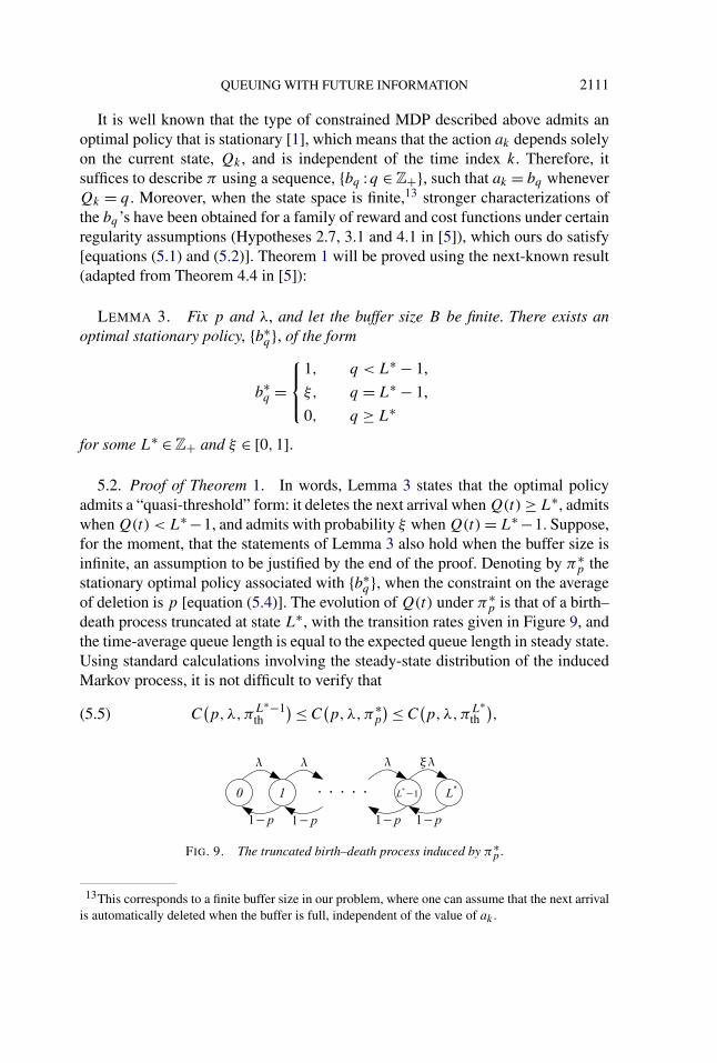
5.2. Proof of Theorem 1. In words, Lemma 3 states that the optimal policyadmits a “quasi-threshold” form: it deletes the next arrival when Q(t) ≥ L∗, admitswhen Q(t) < L∗ −1, and admits with probability ξ when Q(t) = L∗ −1. Suppose,for the moment, that the statements of Lemma 3 also hold when the buffer size isinfinite, an assumption to be justified by the end of the proof. Denoting by π∗
p thestationary optimal policy associated with {b∗
q}, when the constraint on the averageof deletion is p [equation (5.4)]. The evolution of Q(t) under π∗
p is that of a birth–death process truncated at state L∗, with the transition rates given in Figure 9, andthe time-average queue length is equal to the expected queue length in steady state.Using standard calculations involving the steady-state distribution of the inducedMarkov process, it is not difficult to verify that
C(p,λ,πL∗−1
th
) ≤ C(p,λ,π∗
p
) ≤ C(p,λ,πL∗
th),(5.5)
FIG. 9. The truncated birth–death process induced by π∗p .
13This corresponds to a finite buffer size in our problem, where one can assume that the next arrivalis automatically deleted when the buffer is full, independent of the value of ak .
2112 J. SPENCER, M. SUDAN AND K. XU
where L∗ is defined as in Lemma 3, and C(p,λ,π) is the time-average queuelength under policy π , defined in equation (2.9).
Denote by {μLi : i ∈ N} the steady-state probability of the queue length being
equal to i, under a threshold policy πLth . Assuming λ �= 1−p, standard calculations
using the balancing equations yield
μLi =
(λ
1 − p
)i
·(
1 − (λ/(1 − p))
1 − (λ/(1 − p))L+1
)∀1 ≤ i ≤ L(5.6)
and μLi = 0 for all i ≥ L + 1. The time-average queue length is given by
C(p,λ,πL
th) =
L∑i=1
i · μLi
(5.7)
= θ
(θ − 1)(θL+1 − 1)· [
1 − θL + LθL(θ − 1)],
where θ = λ1−p
. Note that when λ > 1 − p, μLi is decreasing with respect to L for
all i ∈ {0,1, . . . ,L} [equation (5.6)], which implies that the time-average queuelength is monotonically increasing in L, that is,
C(p,λ,πL+1
th
) − C(p,λ,πL
th)
= (L + 1) · μL+1L+1 +
L∑i=0
i · (μL+1
i − μLi
)
≥ (L + 1) · μL+1L+1 + L ·
(L∑
i=0
μL+1i − μL
i
)(5.8)
= (L + 1) · μL+1L+1 + L · (
1 − μL+1i − 1
)= μL+1
L+1 > 0.
It is also easy to see that, fixing p, since we have that θ > 1+δ for all λ sufficientlyclose to 1, where δ > 0 is a fixed constant, we have
C(p,λ,πL
th) =
(θL+1
θL+1 − 1
)L − θ
θ − 1· θL − 1
θL+1 − 1∼ L as L → ∞.(5.9)
Since deletions only occur when Q(t) is in state L, from equation (5.6), theaverage rate of deletions in continuous time under πL
th is given by
rd(p,λ,πL
th,) = λ · πL = λ ·
(λ
1 − p
)L
·(
1 − (λ/(1 − p))
1 − (λ/(1 − p))L+1
).(5.10)
Define
L(x,λ) = min{L ∈ Z+ : rd
(p,λ,πL
th,) ≤ x
},(5.11)
QUEUING WITH FUTURE INFORMATION 2113
that is, L(x,λ) is the smallest L for which πLth remains feasible, given a deletion
rate constraint of x. Using equations (5.10) and (5.11) to solve for L(p,λ), weobtain, after some algebra,
L(p,λ) =⌈
logλ/(1−p)
p
1 − λ
⌉∼ log1/(1−p)
1
1 − λas λ → 1(5.12)
and, by combining equation (5.12) and equation (5.9) with L = L(p,λ), we have
C(p,λ,π
L(p,λ)th
) ∼ L(p,λ) ∼ log1/(1−p)
1
1 − λas λ → 1.(5.13)
By equations (5.8) and (5.11), we know that πL(p,λ)th achieves the minimum
average queue length among all feasible threshold policies. By equation (5.5), wemust have that
C(p,λ,π
L(p,λ)−1th
) ≤ C(p,λ,π∗
p
) ≤ C(p,λ,π
L(p,λ)th
).(5.14)
Since Lemma 3 only applies when B < ∞, equation (5.14) holds whenever thebuffer size, B , is greater than L(p,λ), but finite. We next extend equation (5.14)to the case of B = ∞. Denote by ν∗
p a stationary optimal policy, when B = ∞ andthe constraint on average deletion rate is equal to p [equation (5.4)]. The upperbound on C(p,λ,π∗
p) in equation (5.14) automatically holds for C(p,λ, ν∗p), since
C(p,λ,πL(p,λ)th ) is still feasible when B = ∞. It remains to show a lower bound
of the form
C(p,λ, ν∗
p
) ≥ C(p,λ,π
L(p,λ)−2th
),(5.15)
when B = ∞, which, together with the upper bound, will have implied that the
scaling of C(p,λ,πL(p,λ)th ) [equation (5.13)] carries over to ν∗
p ,
C(p,λ, ν∗
p
) ∼ C(p,λ,π
L(p,λ)th
) ∼ log1/(1−p)
1
1 − λas λ → 1,(5.16)
thus proving Theorem 1.To show equation (5.15), we will use a straightforward truncation argument that
relates the performance of an optimal policy under B = ∞ to the case of B < ∞.Denote by {b∗
q} the deletion probabilities of a stationary optimal policy, ν∗p , and by
{b∗q(B ′)} the deletion probabilities for a truncated version, ν∗
p(B ′), with
b∗q
(B ′) = I
(q ≤ B ′) · b∗
q
for all q ≥ 0. Since ν∗p is optimal and yields the minimum average queue length, it
is without loss of generality to assume that the Markov process for Q(t) inducedby ν∗
p is positive recurrent. Denoting by {μ∗i } and {μ∗
i (B′)} the steady-state proba-
bility of queue length being equal to i under ν∗p and ν∗
p(B ′), respectively, it followsfrom the positive recurrence of Q(t) under νp and some algebra, that
limB ′→∞μ∗
i
(B ′) = μ∗
i(5.17)
2114 J. SPENCER, M. SUDAN AND K. XU
for all i ∈ Z+ and
limB ′→∞C
(p,λ, ν∗
p
(B ′)) = C
(p,λ, ν∗
p
).(5.18)
By equation (5.17) and the fact that b∗i (B
′) = b∗i for all 0 ≤ i ≤ B ′, we have that14
limB ′→∞ rd
(p,λ, ν∗
p
(B ′)) = lim
B ′→∞λ
∞∑i=0
μ∗i
(B ′) · (
1 − b∗i
(B ′))
= rd(p,λ, ν∗
p
)(5.19)
≤ p.
It is not difficult to verify, from the definition of L(p,λ) [equation (5.11)], that
limδ→0
L(p + δ, λ) ≥ L(p,λ) − 1,
for all p,λ. For all δ > 0, choose B ′ to be sufficiently large, so that
C(p,λ, ν∗
p
(B ′)) ≤ C
(p,λ, ν∗
p
) + δ,(5.20)
L(λ, rd
(p,λ, ν∗
p
(B ′))) ≥ L(p,λ) − 1.(5.21)
Let p′ = rd(p,λ, ν∗p(B ′)). Since b∗
i (B′) = 0 for all i ≥ B ′ + 1, by equa-
tion (5.21) we have
C(p,λ, ν∗
p
(B ′)) ≥ C
(p,λ,π∗
p′),(5.22)
where π∗p is the optimal stationary policy given in Lemma 3 under any the finite
buffer size B > B ′. We have
C(p,λ, ν∗
p
) + δ
(a)≥ C(p,λ, ν∗
p
(B ′))
(b)≥ C(p,λ,π∗
p′)
(5.23)
(c)≥ C(p,λ,π
L(p′,λ)−1th
)(d)≥ C
(p,λ,π
L(p,λ)−2th
),
where the inequalities (a) through (d) follow from equations (5.20), (5.22), (5.14)and (5.21), respectively. Since equation (5.23) holds for all δ > 0, we have provenequation (5.15). This completes the proof of Theorem 1.
14Note that, in general, rd (p,λ, ν∗p(B ′)) could be greater than p, for any finite B ′.
QUEUING WITH FUTURE INFORMATION 2115
6. Optimal offline policies. We prove Theorem 2 in this section, which iscompleted in two parts. In the first part (Section 6.2), we give a full characterizationof the sample path resulted by applying πNOB (Proposition 1), which turns out tobe a recurrent random walk. This allows us to obtain the steady-state distributionof the queue length under πNOB in closed-form. From this, the expected queuelength, which is equal to the time-average queue length, C(p,λ,πNOB), can beeasily derived and is shown to be 1−p
λ−(1−p). Several side results we obtain along
this path will also be used in subsequent sections.The second part of the proof (Section 6.3) focuses on showing the heavy-traffic
optimality of πNOB among the class of all feasible offline policies, namely, thatlimλ→1 C(p,λ,πNOB) = limλ→1 C∗
�∞(p,λ), which, together with the first part,proves Theorem 2 (Section 6.4). The optimality result is proved using a sample-path-based analysis, by relating the resulting queue length sample path of πNOB tothat of a greedy deletion rule, which has an optimal deletion performance over afinite time horizon, {1, . . . ,N}, given any initial sample path. We then show thatthe discrepancy between πNOB and the greedy policy, in terms of the resultingtime-average queue length after deletion, diminishes almost surely as N → ∞ andλ → 1 (with the two limits taken in this order). This establishes the heavy-trafficoptimality of πNOB.
6.1. Additional notation. Define Q as the resulting queue length process afterapplying πNOB
Q = D(Q0,M�)
and Q as the shifted version of Q, so that Q starts from the first deletion in Q,
Q[n] = Q[n + m�
1], n ∈ Z+.(6.1)
We say that B = {l, . . . , u} ⊂ N is a busy period of Q if
Q[l − 1] = Q[u] = 0 and Q[n] > 0 for all n ∈ {l, . . . , u − 1}.(6.2)
We may write Bj = {lj , . . . , uj } to mean the j th busy period of Q. An example ofa busy period is illustrated in Figure 6.
Finally, we will refer to the set of slots between two adjacent deletions in Q
(note the offset of m1),
Ei = {m�
i − m�1 ,m�
i + 1 − m�1 , . . . ,m�
i+1 − 1 − m�1
}(6.3)
as the ith deletion epoch.
6.2. Performance of the no-job-left-behind policy. For simplicity of notation,throughout this section, we will denote by M = {mi : i ∈ N} the deletion sequencegenerated by applying πNOB to Q0, when there is no ambiguity (as opposed tousing M� and m�
i ). The following lemma summarizes some important propertiesof Q which will be used repeatedly.
2116 J. SPENCER, M. SUDAN AND K. XU
LEMMA 4. Suppose 1 > λ > 1 − p > 0. The following hold with probabilityone:
(1) For all n ∈ N, we have Q[n] = Q0[n + m1] − I (M,n + m1).(2) For all i ∈ N, we have n = mi − m1, if and only if
Q[n] = Q[n − 1] = 0(6.4)
with the convention that Q[−1] = 0. In other words, the appearance of two con-secutive zeros in Q is equivalent to having a deletion on the second zero.
(3) Q[n] ∈ Z+ for all n ∈ Z+.
PROOF. See Appendix A.2 �
The next proposition is the main result of this subsection. It specifies the prob-ability law that governs the evolution of Q.
PROPOSITION 1. {Q[n] :n ∈ Z+} is a random walk on Z+, with Q[0] = 0,and, for all n ∈ N and x1, x2 ∈ Z+,
P(Q[n + 1] = x2|Q[n] = x2
) =
⎧⎪⎪⎪⎪⎪⎪⎨⎪⎪⎪⎪⎪⎪⎩
1 − p
λ + 1 − p, x2 − x1 = 1,
λ
λ + 1 − p, x2 − x1 = −1,
0, otherwise,if x1 > 0 and
P(Q[n + 1] = x2|Q[n] = x1
) =
⎧⎪⎪⎪⎪⎪⎪⎨⎪⎪⎪⎪⎪⎪⎩
1 − p
λ + 1 − p, x2 − x1 = 1,
λ
λ + 1 − p, x2 − x1 = 0,
0, otherwise,if x1 = 0.
PROOF. For a sequence {X[n] :n ∈ N} and s, t ∈ N, s ≤ t , we will use theshorthand
Xts = {
X[s], . . . ,X[t]}.Fix n ∈ N , and a sequence (q1, . . . , qn) ⊂ Z
n+. We have
P(Q[n] = q[n]|Qn−1
1 = qn−11
)=
n∑k=1
∑t1,...,tk,
tk≤n−1+t1
P(Q[n] = q[n]|Qn−1
1 = qn−11 ,mk
1 = tk1 ,mk+1 ≥ n + t1)
(6.5)
× P(mk
1 = tk1 ,mk+1 ≥ n + t1|Qn−11 = qn−1
1
).
QUEUING WITH FUTURE INFORMATION 2117
Restricting to the values of ti ’s and q[i]’s under which the summand is nonzero,the first factor in the summand can be written as
where Q was defined in equation (6.1). Step (a) follows from Lemma 4 and thefact that tk ≤ n − 1 + t1, and (b) from the Markov property of Q0 and the fact thatthe events {minr≥n+t1 Q0[r] ≥ k}, {Q0[n + t1] = q[n] + k} and their intersection,depend only on the values of {Q0[s] : s ≥ n + t1}, and are hence independent of{Q0[s] : 1 ≤ s ≤ n − 2 + t1} conditional on the value of Q0[t1 + n − 1].
Since the process Q lives in Z+ (Lemma 4), it suffices to consider the case ofq[n] = q[n − 1] + 1, and show that
for all q[n − 1] ∈ Z+. Since Q[mi − m1] = Q[mi − 1 − m1] = 0 for all i
(Lemma 4), the fact that q[n] = q[n − 1] + 1 > 0 implies that
n < mk+1 − 1 + m1.(6.8)
Moreover, since Q0[mk+1 − 1] = k and n < mk+1 − 1 + m1, we have that
q[n] > 0 implies Q0[t] = k for some t ≥ n + 1 + m1.(6.9)
We consider two cases, depending on the value of q[n − 1].Case 1: q[n − 1] > 0. Using the same argument that led to equation (6.9), we
have that
q[n − 1] > 0 implies Q0[t] = k for some t ≥ n + m1.(6.10)
2118 J. SPENCER, M. SUDAN AND K. XU
It is important to note that, despite the similarity of their conclusions, equa-tions (6.9) and (6.10) are different in their assumptions (i.e., q[n] versus q[n− 1]).We have
where (a) follows from equation (6.10), (b) from the stationary and space-homogeneity of the Markov chain Q0 and (c) from the following well-knownproperty of a transient random walk conditional to returning to zero:
LEMMA 5. Let {X[n] :n ∈ N} be a random walk on Z+, such that for allx1, x2 ∈ Z+ and n ∈ N,
P(X[n + 1] = x2|X[n] = x2
) =⎧⎪⎨⎪⎩
q, x2 − x1 = 1,
1 − q, x2 − x1 = −1,
0, otherwise,
if x1 > 0 and
P(X[n + 1] = x2|X[n] = x1
) =⎧⎪⎨⎪⎩
q, x2 − x1 = 1,
1 − q, x2 − x1 = 0,
0, otherwise,
if x1 = 0, where q ∈ (12 ,1). Then for all x1, x2 ∈ Z+ and n ∈N,
P
(X[n + 1] = x2|X[n] = x1, min
r≥n+1X[r] = 0
)=
⎧⎪⎨⎪⎩1 − q, x2 − x1 = 1,
q, x2 − x1 = −1,
0, otherwise,
if x1 > 0 and
P
(X[n + 1] = x2|X[n] = x1, min
r≥n+1X[r] = 0
)=
⎧⎪⎨⎪⎩1 − q, x2 − x1 = 1,
q, x2 − x1 = 0,
0, otherwise,
QUEUING WITH FUTURE INFORMATION 2119
if x1 = 0. In other words, conditional on the eventual return to 0 and before ithappens, a transient random walk obeys the same probability law as a randomwalk with the reversed one-step transition probability.
where (a) follows from equation (6.9) [note its difference with equation (6.10)],and (b) from the stationarity and space-homogeneity of Q0, and the assumptionthat k ≥ 1 [equation (6.5)].
Since equations (6.11) and (6.12) hold for all x1, k ∈ Z+ and n ≥ m1 + 1, byequation (6.5), we have that
P(Q[n] = q[n]|Qn−1
1 = qn−11
)(6.13)
=
⎧⎪⎪⎪⎪⎪⎪⎨⎪⎪⎪⎪⎪⎪⎩
1 − p
λ + 1 − p, q[n] − q[n − 1] = 1,
λ
λ + 1 − p, q[n] − q[n − 1] = −1,
0, otherwise,
if q[n − 1] > 0 and
P(Q[n] = q[n]|Qn−1
1 = qn−11
) =⎧⎪⎨⎪⎩
x, q[n] − q[n − 1] = 1,
1 − x, q[n] − q[n − 1] = 0,
0, otherwise,
(6.14)
if q[n − 1] = 0, where x represents the value of the probability in equation (6.12).Clearly, Q[0] = Q0[m1] = 0. We next show that x is indeed equal to 1−p
λ+1−p, which
will have proven Proposition 1.
2120 J. SPENCER, M. SUDAN AND K. XU
One can in principle obtain the value of x by directly computing the probabilityin line (b) of equation (6.12), which can be quite difficult to do. Instead, we willuse an indirect approach that turns out to be computationally much simpler: wewill relate x to the rate of deletion of πNOB using renewal theory, and then solvefor x. As a by-product of this approach, we will also get a better understandingof an important regenerative structure of πNOB [equation (6.20)], which will beuseful for the analysis in subsequent sections.
By equations (6.13) and (6.14), Q is a positive recurrent Markov chain, andQ[n] converges to a well-defined steady-state distribution, Q[∞], as n → ∞. Let-ting πi = P(Q[∞] = i), it is easy to verify via the balancing equations that
πi = π0x(λ + 1 − p)
λ·(
1 − p
λ
)i−1
∀i ≥ 1(6.15)
and since∑
i≥0 πi = 1, we obtain
π0 = 1
1 + x · (λ + 1 − p)/(λ − (1 − p)).(6.16)
Since the chain Q is also irreducible, the limiting fraction of time that Q spendsin state 0 is therefore equal to π0,
limn→∞
1
n
n∑t=1
I(Q[t] = 0
) = π0 = 1
1 + x · (λ + 1 − p)/(λ − (1 − p)).(6.17)
Next, we would like to know many of these visits to state 0 correspond to adeletion. Recall the notion of a busy period and deletion epoch, defined in equa-tions (6.2) and (6.3), respectively. By Lemma 4, n corresponds to a deletion if anyonly if Q[n] = Q[n − 1] = 0. Consider a deletion in slot mi . If Q[mi + 1] = 0,then mi + 1 also corresponds to a deletion, that is, mi + 1 = mi+1. If insteadQ[mi + 1] = 1, which happens with probability x, the fact that Q[mi+1 − 1] = 0implies that there exists at least one busy period, {l, . . . , u}, between mi and mi+1,with l = mi and u ≤ mi+1 − 1. At the end of this period, a new busy period startswith probability x and so on. In summary, a deletion epoch Ei consists of the slotmi − m1, plus Ni busy periods, where the Ni are i.i.d., with15
N1d= Geo(1 − x) − 1(6.18)
and hence
|Ei | = 1 +Ni∑
j=1
Bi,j ,(6.19)
where {Bi,j : i, j ∈ N} are i.i.d. random variables, and Bi,j corresponds to thelength of the j th busy period in the ith epoch.
15Geo(p) denotes a geometric random variable with mean 1p .
QUEUING WITH FUTURE INFORMATION 2121
Define W [t] = (Q[t],Q[t + 1]), t ∈ Z+. Since Q is Markov, W [t] is also aMarkov chain, taking values in Z
2+. Since a deletion occurs in slot t if and only ifQ[t] = Q[t −1] = 0 (Lemma 4), |Ei | corresponds to excursion times between twoadjacent visits of W to the state (0,0), and hence are i.i.d. Using the elementaryrenewal theorem, we have
limn→∞
1
nI (M,n) = 1
E(|E1|) a.s.(6.20)
and by viewing each visit of W to (0,0) as a renewal event and using the fact thatexactly one deletion occurs within a deletion epoch. Denoting by Ri the number ofvisits to the state 0 within Ei , we have that Ri = 1 +Ni . Treating Ri as the rewardassociated with the renewal interval Ei , we have, by the time-average of a renewalreward process (cf. Theorem 6, Chapter 3, [10]), that
limn→∞
1
n
n∑t=1
I(Q[t] = 0
) = E(R1)
E(|E1|) = E(N1) + 1
E(|E1|) a.s.(6.21)
by treating each visit of Q to (0,0) as a renewal event. From equations(6.20) and (6.21), we have
limn→∞(1/n)I (M,n)
limn→∞(1/n)∑n
t=1 I(Q[t] = 0)= 1
E(N1)= 1 − x.(6.22)
Combining equations (4.1), (6.17) and (6.22), and the fact that E(N1) = E(Geo(1−x)) − 1 = 1
1−x− 1, we have
λ − (1 − p)
λ + 1 − p·[1 + x · λ + 1 − p
λ − (1 − p)
]= 1 − x,(6.23)
which yields
x = 1 − p
λ + 1 − p.(6.24)
This completes the proof of Proposition 1. �
We summarize some of the key consequences of Proposition 1 below, mostof which are easy to derive using renewal theory and well-known properties ofpositive-recurrent random walks.
PROPOSITION 2. Suppose that 1 > λ > 1 − p > 0, and denote by Q[∞] thesteady-state distribution of Q.
(1) For all i ∈ Z+,
P(Q[∞] = i
) =(
1 − 1 − p
λ
)·(
1 − p
λ
)i
.(6.25)
2122 J. SPENCER, M. SUDAN AND K. XU
(2) Almost surely, we have that
limn→∞
1
n
n∑i=1
Q[i] = E(Q[∞]) = 1 − p
λ − (1 − p).(6.26)
(3) Let Ei = {m�i ,m�
i + 1, . . . ,m�i+1 − 1,m�
i+1}. Then the |Ei | are i.i.d., with
E(|E1|) = 1
limn→∞(1/n)I (M�,n)= λ + 1 − p
λ − (1 − p)(6.27)
and there exists a, b > 0 such that for all x ∈ R+
P(|E1| ≥ x
) ≤ a · exp(−b · x).(6.28)
(4) Almost surely, we have that
m�i ∼ 1
E(|E1|) · i = λ − (1 − p)
λ + 1 − p· i(6.29)
as i → ∞.
PROOF. Claim 1 follows from the well-known steady-state distribution of arandom walk, or equivalently, the fact that Q[∞] has the same distribution as thesteady-state number of jobs in an M/M/1 queue with traffic intensity ρ = 1−p
λ.
For Claim 2, since Q is an irreducible Markov chain that is positive recurrent, itfollows that its time-average coincides with E(Q[∞]) almost surely.
The fact that Ei ’s are i.i.d. was shown in the discussion preceding equa-tion (6.20) in the proof of Proposition 1. The value of E(|E1|) follows by com-bining equations (4.1) and (6.20).
Let Bi,j be the length of the j th busy period [defined in equation (6.2)] in Ei .By definition, B1,1 is distributed as the time till the random walk Q reaches state0, starting from state 1. We have
P(B1,1 ≥ x) ≤ P
( �x�∑j=1
Xj ≤ −1
),
where the Xj ’s are i.i.d., with P(X1 = 1) = 1−pλ+1−p
and P(X1 = −1) = λλ+1−p
,which, by the Chernoff bound, implies an exponential tail bound for P(B1,1 ≥ x),and in particular,
limθ↓0
GB1,1(θ) = 1.(6.30)
QUEUING WITH FUTURE INFORMATION 2123
By equation (6.19), the moment generating function for |E1| is given by
G|E1|(ε) = E(exp
(ε · |E1|))
= E
(exp
(ε ·
(1 +
N1∑j=1
B1,j
)))(6.31)
(a)= E(eε) ·E(
exp(N1 · GB1,1(ε)
))= E
(eε) · GN1
(ln
(GB1,1(ε)
)),
where (a) follows from the fact that {N1}∪{B1,j : j ∈N} are mutually independent,
and GN1(x) = E(exp(x · N1)). Since N1d= Geo(1 − x) − 1, limx↓0 GN1(x) = 1,
and by equation (6.30), we have that limε↓0 G|E1|(ε) = 1, which implies equa-tion (6.28).
Finally, equation (6.29) follows from the third claim and the elementary renewaltheorem. �
6.3. Optimality of the no-job-left-behind policy in heavy traffic. This sectionis devoted to proving the optimality of πNOB as λ → 1, stated in the second claimof Theorem 2, which we isolate here in the form of the following proposition.
PROPOSITION 3. Fix p ∈ (0,1). We have that
limλ→1
C(p,λ,πNOB) = limλ→1
C∗�∞(p,λ).
The proof is given at the end of this section, and we do so by showing thefollowing:
(1) Over a finite horizon N and given a fixed number of deletions to be made,a greedy deletion rule is optimal in minimizing the post-deletion area under Q over{1, . . . ,N}.
(2) Any point of deletion chosen by πNOB will also be chosen by the greedypolicy, as N → ∞.
(3) The fraction of points chosen by the greedy policy but not by πNOB dimin-ishes as λ → 1, and hence the delay produced by πNOB is the best possible, asλ → 1.
Fix N ∈ N. Let S(Q,N) be the partial sum S(Q,N) = ∑Nn=1 Q[n]. For any
sample path Q, denote by �(Q,n) the marginal decrease of area under Q over thehorizon {1, . . . ,N} by applying a deletion at slot n, that is,
�P (Q,N,n) = S(Q,N) − S(DP (Q,n),N
)and, analogously,
�(Q,N,M ′) = S(Q,N) − S
(D
(Q,M ′),N)
,
2124 J. SPENCER, M. SUDAN AND K. XU
where M ′ is a deletion sequence.We next define the notion of a greedy deletion rule, which constructs a dele-
tion sequence by recursively adding the slot that leads to the maximum marginaldecrease in S(Q,N).
DEFINITION 9 (Greedy deletion rule). Fix an initial sample path Q0 andK,N ∈ N. The greedy deletion rule is a mapping, G(Q0,N,K), which outputsa finite deletion sequence MG = {mG
i : 1 ≤ i ≤ K}, given by
mG1 ∈ arg max
m∈�(Q0,N)�P
(Q0,N,m
),
mGk ∈ arg max
m∈�(Qk−1,N)�P
(Qk−1
MG ,N,m), 2 ≤ k ≤ K,
where �(Q,N) = �(Q) ∩ {1, . . . ,N} is the set of all locations in Q in the firstN slots that can be deleted, and Qk
MG = D(Q0, {mGi : 1 ≤ i ≤ k}). Note that
we will allow mGk = ∞, if there is no more entry to delete [i.e., �(Qk−1) ∩
{1, . . . ,N} =∅].
We now state a key lemma that will be used in proving Theorem 2. It shows thatover a finite horizon and for a finite number of deletions, the greedy deletion ruleyields the maximum reduction in the area under the sample path.
LEMMA 6 (Dominance of greedy policy). Fix an initial sample path Q0, hori-zon N ∈ N and number of deletions K ∈ N. Let M ′ be any deletion sequence withI (M ′,N) = K . Then
S(D
(Q0,M ′),N) ≥ S
(D
(Q0,MG)
,N),
where MG = G(Q0,N,K) is the deletion sequence generated by the greedy pol-icy.
PROOF. By Lemma 1, it suffices to show that, for any sample path {Q[n] ∈Z+ :n ∈ N} with |Q[n+1]−Q[n]| = 1 if Q[n] > 0 and |Q[n+1]−Q[n]| ∈ {0,1}if Q[n] = 0, we have
S(D
(Q,M ′),N)
(6.32)≥ �P
(Q,N,mG
1) + min
|M|=k−1,
M⊂�(D(Q,mG1 ),N)
S(D
(Q1
MG, M),N
).
By induction, this would imply that we should use the greedy rule at every step ofdeletion up to K . The following lemma states a simple monotonicity property. Theproof is elementary, and is omitted.
QUEUING WITH FUTURE INFORMATION 2125
LEMMA 7 (Monotonicity in deletions). Let Q and Q′ be two sample pathssuch that
Q[n] ≤ Q′[n] ∀n ∈ {1, . . . ,N}.Then, for any K ≥ 1,
min|M|=K,
M⊂�(Q,N)
S(D(Q,M),N
) ≤ min|M|=K,
M⊂�(Q′,N)
S(D
(Q′,M
),N
)(6.33)
and, for any finite deletion sequence M ′ ⊂ �(Q,N),
�(Q,N,M ′) ≥ �
(Q′,N,M ′).(6.34)
Recall the definition of a busy period in equation (6.2). Let J (Q,N) be thetotal number of busy periods in {Q[n] : 1 ≤ n ≤ N}, with the additional convention
Q[N +1] �= 0 so that the last busy period always ends on N . Let Bj = {lj , . . . , uj }be the j th busy period. It can be verified that a deletion in location n leads to adecrease in the value of S(Q,N) that is no more than the width of the busy periodto which n belongs; cf. Figure 6. Therefore, by definition, a greedy policy alwaysseeks to delete in each step the first arriving job during a longest busy period in thecurrent sample path, and hence
�(Q,N,G(Q,N,1)
) = max1≤j≤J (Q,N)
|Bj |.(6.35)
Let
J ∗(Q,N) = arg max1≤j≤J (Q,N)
|Bj |.
We consider the following cases, depending on whether M ′ chooses to delete anyjob in the busy periods in J ∗(Q,N).
Case 1: M ′ ∩ (⋃
j∈J ∗(Q,N) Bj ) �= ∅. If lj∗ ∈ M ′ for some j∗ ∈ J ∗, by equa-tion (6.35), we can set mG
1 to lj∗ . Since mG1 ∈ M ′ and the order of deletions does
not impact the final resulting delay (Lemma 1), we have that equation (6.32) holds,and we are done. Otherwise, choose m∗ ∈ M ′ ∩Bj∗ for some j∗ ∈ J ∗, and we havem∗ > lj∗ . Let
Q′ = DP
(Q,m∗)
and Q = DP (Q, lj∗).
Since Q[n] > 0, ∀n ∈ {lj∗, . . . , uj∗ − 1}, we have Q[n] = Q[n] − 1 ≤ Q′[n],∀n ∈ {lj∗, . . . , uj∗ − 1} and Q′[n] = Q[n] = Q[n], ∀n /∈ {lj∗, . . . , uj∗ − 1}, whichimplies that
Q[n] ≤ Q′[n] ∀n ∈ {1, . . . ,N}.(6.36)
Equation (6.32) holds by combining equation (6.36) and equation (6.33) inLemma 7, with K = k − 1.
2126 J. SPENCER, M. SUDAN AND K. XU
Case 2: M ′ ∩ (⋃
j∈J ∗(Q,N) Bj ) = ∅. Let m∗ be any element in M ′ and Q′ =DP (Q,m∗). Clearly, Q[n] ≥ Q′[n] for all n ∈ {1, . . . ,N}, and by equation (6.34)in Lemma 7, we have that16
�(Q,N,M ′ \ {
m∗}) ≥ �(DP
(Q,m∗)
,N,M ′ \ {m∗})
.(6.37)
Since M ′ ∩ (⋃
j∈J ∗(Q,N) Bj ) = ∅, we have that
�P
(D
(Q,M ′ \ {
m∗}),N,mG
1) = max
1≤j≤J (Q,N)|Bj | > �P
(Q,N,m∗)
.(6.38)
Let M = mG1 ∪ (M ′ \ {m∗}), and we have that
S(D(Q,M),N
)= S(Q,N) − �
(Q,N,M ′ \ {
m∗}) − �P
(D
(Q,M ′ \ {
m∗}),N,mG
1)
(a)≤ S(Q,N) − �(DP
(Q,m∗)
,N,M ′ \ {m∗})
− �P
(D
(Q,M ′ \ {
m∗}),N,mG
1)
(b)< S(Q,N) − �
(DP
(Q,m∗)
,N,M ′ \ {m∗}) − �P
(Q,N,m∗)
= S(D
(Q,M ′),N)
,
where (a) and (b) follow from equations (6.37) and (6.38), respectively, whichshows that equation (6.32) holds (and in this case the inequality there is strict).
Cases 1 and 2 together complete the proof of Lemma 6. �
We are now ready to prove Proposition 3.
PROOF OF PROPOSITION 3. Lemma 6 shows that, for any fixed number ofdeletions over a finite horizon N , the greedy deletion policy (Definition 9) yieldsthe smallest area under the resulting sample path, Q, over {1, . . . ,N}. The mainidea of proof is to show that the area under Q after applying πNOB is asymptoti-cally the same as that of the greedy policy, as N → ∞ and λ → 1 (in this particularorder of limits). In some sense, this means that the jobs in M� account for almostall of the delays in the system, as λ → 1. The following technical lemma is useful.
LEMMA 8. For a finite set S ⊂R and k ∈ N, define
f (S, k) = sum of the k largest elements in S
|S| .
Let {Xi : 1 ≤ i ≤ n} be i.i.d. random variables taking values in Z+, whereE(X1) < ∞. Then for any sequence of random variables {Hn :n ∈ N}, with
16For finite sets A and B , A \ B = {a ∈ A :a /∈ B}.
QUEUING WITH FUTURE INFORMATION 2127
Hn � αn a.s. as n → ∞ for some α ∈ (0,1), we have
lim supn→∞
f({Xi : 1 ≤ i ≤ n},Hn
) ≤ E(X1 · I(X1 ≥ �F−1
X1(α)
))a.s.,(6.39)
where �F−1X1
(y) = min{x ∈ N :P(X1 ≥ x) < y}.
PROOF. See Appendix A.4. �
Fix an initial sample path Q0. We will denote by M� = {m�i : i ∈ N} the dele-
tion sequence generated by πNOB on Q0. Define
l(n) = n − max1≤i≤I (M�,n)
|Ei |,(6.40)
where Ei is the ith deletion epoch of M� , defined in equation (6.3). Since Q0[n] ≥Q0[mi] for all i ∈N, it is easy to check that
�P
(D
(Q0,
{m�
j : 1 ≤ j ≤ i − 1})
, n,m�i
) = n − m�i + 1
for all i ∈ N. The function l was defined so that the first I (M�, l(n)) deletionsmade by a greedy rule over the horizon {1, . . . , n} are exactly {1, . . . , l(n)} ∩ M� .More formally, we have the following lemma.
LEMMA 9. Fix n ∈ N, and let MG = G(Q0, n, I (M�, l(n))). Then mGi =
m�i , for all i ∈ {1, . . . , I (M�, l(n))}.
Fix K ∈ N, and an arbitrary feasible deletion sequence, M , generated by a pol-icy in �∞. We can write
I(M,m�
K
) = I(M�, l
(m�
K
)) + (I(M�,m�
K
) − I(M�, l
(m�
K
)))+ (
I(M,m�
K
) − I(M�,m�
K
))= I
(M�, l
(m�
K
)) + (K − I
(M�, l
(m�
K
)))(6.41)
+ (I(M,m�
K
) − I(M�,m�
K
))= I
(M�, l
(m�
K
)) + h(K),
where
h(K) = (K − I
(M�, l
(m�
K
))) + (I(M,m�
K
) − I(M�,m�
K
)).(6.42)
We have the following characterization of h.
LEMMA 10. h(K)� 1−λλ−(1−p)
· K , as K → ∞, a.s.
PROOF. See Appendix A.5. �
2128 J. SPENCER, M. SUDAN AND K. XU
Let
MG,n = G(Q0, n, I (M, n)
),(6.43)
where the greedy deletion map G was defined in Definition 9. By Lemma 9 andthe definition of MG,n, we have that
M� ∩ {1, . . . , l
(m�
K
)} ⊂ MG,m�K .(6.44)
Therefore, we can write
MG,m�K = (
M� ∩ {1, . . . , l
(m�
K
)}) ∪ �MGK,(6.45)
where �MGK
�= MG,m�K \ (M� ∩ {1, . . . , l(m�
K)}). Since |MG,m�K | = I (M,m�
K) bydefinition, by equation (6.41), ∣∣ �MG
K
∣∣ = h(K).(6.46)
We have
S(D
(Q0,M�)
,m�K
) − S(D
(Q0, M
),m�
K
)(a)≤ S
(D
(Q0,M�)
,m�K
) − S(D
(Q0,MG,m�
K),m�
K
)(6.47)
(b)= �(D
(Q0,M�)
,m�K, �MG
K
),
where (a) is based on the dominance of the greedy policy over any finite horizon(Lemma 6), and (b) follows from equation (6.45).
Finally, we claim that there exists g(x) :R → R+, with g(x) → 0 as x → 1,such that
lim supK→∞
�(D(Q0,M�),m�K, �MG
K)
m�K
≤ g(λ) a.s.(6.48)
Equations (6.47) and (6.48) combined imply that
C(p,λ,πNOB) = lim supK→∞
S(D(Q0,M�),m�K)
m�K
≤ g(λ) + lim supK→∞
S(D(Q0, M),m�K)
m�K
,(6.49)
= g(λ) + lim supn→∞
S(D(Q0, M), n)
na.s.,
which shows that
C(p,λ,πNOB) ≤ g(λ) + infπ∈�∞
C(p,λ,π).
Since g(λ) → 0 as λ → 1, this proves Proposition 3.To show equation (6.48), denote by Q the sample path after applying πNOB,
Q = D(Q0,M�)
QUEUING WITH FUTURE INFORMATION 2129
and by Vi the area under Q within Ei ,
Vi =m�
i+1−1∑n=m�
i
Q[n].
An example of Vi is illustrated as the area of the shaded region in Figure 6.By Proposition 1, Q is a Markov chain, and so is the process W [n] = (Q[n],Q[n + 1]). By Lemma 4, Ei corresponds to the indices between two adjacent re-turns of the chain W to state (0,0). Since the ith return of a Markov chain to aparticular state is a stopping time, it can be shown, using the strong Markov prop-erty of W , that the segments of Q, {Q[n] :n ∈ Ei}, are mutually independent andidentically distributed among different values of i. Therefore, the Vi’s are i.i.d.Furthermore,
E(V1)(a)≤ E
(|E1|2) (b)< ∞,(6.50)
where (a) follows from the fact that |Q[n + 1] − Q[n]| ≤ 1 for all n, and henceVi ≤ |Ei |2 for any sample path of Q0, and (b) from the exponential tail bound onP(|E1| ≥ x), given in equation (6.28).
Since the value of Q on the two ends of Ei , m�i and m�
i+1 − 1, areboth zero, each additional deletion within Ei cannot produce a marginal de-crease of area under Q of more than Vi ; cf. Figure 6. Therefore, the valueof �(D(Q0,M�),m�
K, �MGK) can be no greater than the sum of the h(K) largest
Vi’s over the horizon n ∈ {1, . . . ,m�K}. We have
lim supK→∞
�(D(Q0,M�),m�K, �MG
K)
m�K
= lim supK→∞
f({Vi : 1 ≤ i ≤ K}, h(K)
) · K
m�K
(6.51)(a)= lim sup
K→∞f
({Vi : 1 ≤ i ≤ K}, h(K)) · λ + 1 − p
λ − (1 − q)
(b)= E
(V1 · I
(X1 ≥ �F−1
V1
(1 − λ
λ − (1 − p)
)))· λ + 1 − p
λ − (1 − q),
where (a) follows from equation (6.29), and (b) from Lemmas 8 and 10. SinceE(V1) < ∞, and �F−1
V1(x) → ∞ as x → 0, it follows that
E
(V1 · I
(X1 ≥ �F−1
V1
(1 − λ
λ − (1 − p)
)))→ 0
as λ → 1. Equation (6.48) is proved by setting
g(λ) = E
(V1 · I
(X1 ≥ �F−1
V1
(1 − λ
λ − (1 − p)
)))· λ + 1 − p
λ − (1 − q).
This completes the proof of Proposition 3. �
2130 J. SPENCER, M. SUDAN AND K. XU
6.3.1. Why not use greedy? The proof of Proposition 3 relies on a sample-path-wise coupling to the performance of a greedy deletion rule. It is then onlynatural to ask: since the time horizon is indeed finite in all practical applications,why do not we simply use the greedy rule as the preferred offline policy, as opposedto πNOB?
There are at least two reasons for focusing on πNOB instead of the greedy rule.First, the structure of the greedy rule is highly global, in the sense that each deletiondecision uses information of the entire sample path over the horizon. As a result,the greedy rule tells us little on how to design a good policy with a fixed looka-head window (e.g., Theorem 3). In contrast, the performance analysis of πNOB inSection 6.2 reveals a highly regenerative structure: the deletions made by πNOB
essentially depend only on the dynamics of Q0 in the same deletion epoch (theEi ’s), and what happens beyond the current epoch becomes irrelevant. This is thekey intuition that led to our construction of the finite-lookahead policy in Theo-rem 3. A second (and perhaps minor) reason is that of computational complexity.By a small sacrifice in performance, πNOB can be efficiently implemented using alinear-time algorithm (Section 4.2), while it is easy to see that a naive implemen-tation of the greedy rule would require super-linear complexity with respect to thelength of the horizon.
6.4. Proof of Theorem 2. The fact that πNOB is feasible follows from equa-tion (4.1) in Lemma 2, that is,
lim supn→∞
1
nI(M�,n
) ≤ λ − (1 − p)
λ + 1 − p<
p
λ + 1 − pa.s.
Let {Q[n] :n ∈ Z+} be the resulting sample path after applying πNOB to theinitial sample path {Q0[n] :n ∈ Z+}, and let
Q[n] = Q[n + m�
1] ∀n ∈ N,
where m�1 is the index of the first deletion made by πNOB. Since λ > 1 − p, the
random walk Q0 is transient, and hence m�1 < ∞ almost surely. We have that,
almost surely,
C(p,λ,πNOB) = limn→∞
1
n
n∑i=1
Q[i]
= limn→∞
1
n
m�1∑
i=1
Q[i] + limn→∞
1
n
n∑i=1
Q[i](6.52)
= 1 − p
λ − (1 − p),
QUEUING WITH FUTURE INFORMATION 2131
where the last equality follows from equation (6.26) in Proposition 2, and the factthat m1 < ∞ almost surely. Letting λ → 1 in equation (6.52) yields the finite limitof delay under heavy traffic,
limλ→1
C(p,λ,πNOB) = limλ→1
1 − p
λ − (1 − p)= 1 − p
p.
Finally, the delay optimality of πNOB in heavy traffic was proved in Proposi-tion 3, that is, that
limλ→1
C(p,λ,πNOB) = limλ→1
C∗�∞(p,λ).
This completes the proof of Theorem 2.
7. Policies with a finite lookahead.
7.1. Proof of Theorem 3. As pointed out in the discussion preceding Theo-rem 3, for any initial sample path and w < ∞, an arrival that is deleted under theπNOB policy will also be deleted under πw
NOB. Therefore, the delay guarantee for
πNOB (Theorem 2) carries over to πw(λ)NOB , and for the rest of the proof, we will be
focusing on showing that πw(λ)NOB is feasible under an appropriate scaling of w(λ).
We begin by stating an exponential tail bound on the distribution of the discrete-time predictive window, W(λ,n), defined in equation (3.6),
W(λ,n) = max{k ∈ Z+ :Tn+k ≤ Tn + w(λ)
}.
It is easy to see that {W(λ,m�i ) : i ∈ N} are i.i.d., with W(λ,m�
1 ) distributed as aPoisson random variable with mean (λ + 1 − p)w(λ). Since
P(W
(λ,m�
1) ≥ x
) ≤ P
(�w(λ)�∑k=1
Xk
),
where the Xk are i.i.d. Poisson random variables with mean λ + (1 − p), applyingthe Chernoff bound, we have that, there exist c, d > 0 such that
P
(W
(λ,m�
1) ≥ λ + 1 − p
2· w(λ)
)≤ c · exp
(−d · w(λ))
(7.1)
for all w(λ) > 0.We now analyze the deletion rate resulted by the π
w(λ)NOB policy. For the pure
purpose of analysis (as opposed to practical efficiency), we will consider a newdeletion policy, denoted by σw(λ), which can be viewed as a relaxation of π
w(λ)NOB .
DEFINITION 10. Fix w ∈ R+. The deletion policy σw is defined such that foreach deletion epoch Ei , i ∈N:
2132 J. SPENCER, M. SUDAN AND K. XU
(1) if |Ei | ≤ W(λ,m�i ), then only the first arrival of this epoch, namely, the
arrival in slot m�i , is deleted;
(2) otherwise, all arrivals within this epoch are deleted.
It is easy to verify that σw can be implemented with w units of look-ahead,and the set of deletions made by σw(λ) is a strict superset of π
w(λ)NOB almost surely.
Hence, the feasibility of σw(λ) will imply that of πw(λ)NOB .
Denote by Di the number of deletions made by σw(λ) in the epoch Ei . By theconstruction of the policy, the Di are i.i.d., and depend only on the length of Ei
and the number of arrivals within. We have17
E(D1) ≤ 1 +E[|Ei | · I(|Ei | ≥ W
(λ,m�
i
))]≤ 1 +E
[|Ei | · I
(|Ei | ≥ λ + 1 − p
2· w(λ)
)]+E
(|Ei |) · P(W
(λ,m�
i
) ≤ λ + 1 − p
2· w(λ)
)(7.2)
≤ 1 +( ∞∑
k=((λ+1−p)/2)·w(λ)
k · a · exp(−b · k)
)
+ λ
λ − (1 − p)· c · exp
(−d · w(λ))
(a)≤ 1 + h · w(λ) · exp(−l · w(λ)
)for some h, l > 0, where (a) follows from the fact that
∑∞k=n k · exp(−b · k) =
O(n · exp(−b · n)) as n → ∞.Since the Di are i.i.d., using basic renewal theory, it is not difficult to show
that the average rate of deletion in discrete time under the policy σw(λ) is equal toE(D1)E(E1)
. In order for the policy to be feasible, one must have that
E(D1)
E(E1)= E(D1)
λ≤ p
λ + 1 − p.(7.3)
By equations (7.2) and (7.3), we want to ensure that
pλ
λ − (1 − p)≥ 1 + h · w(λ) · exp
(−l · w(λ)),
which yields, after taking the logarithm on both sides,
w(λ) ≥ 1
blog
(1
1 − λ
)+ 1
blog
( [λ − (1 − p)] · h · w(λ)
1 − p
).(7.4)
17For simplicity of notation, we assume that λ+1−p2 · w(λ) is always an integer. This does not
change the scaling behavior of w(λ).
QUEUING WITH FUTURE INFORMATION 2133
It is not difficult to verify that for all p ∈ (0,1) there exists a constant C such thatthe above inequality holds for all λ ∈ (1 − p,1), by letting w(λ) = C log( 1
1−λ).
This proves the feasibility of σw(λ), which implies that πw(λ)NOB is also feasible. This
completes the proof of Theorem 3.
8. Concluding remarks and future work. The main objective of this paperis to study the impact of future information on the performance of a class of admis-sions control problems, with a constraint on the time-average rate of redirection.Our model is motivated as a study of a dynamic resource allocation problem be-tween slow (congestion-prone) and fast (congestion-free) processing resources. Itcould also serve as a simple canonical model for analyzing delays in large serverfarms or cloud clusters with resource pooling [20]; cf. Appendix B. Our main re-sults show that the availability of future information can dramatically reduce thedelay experienced by admitted customer: the delay converges to a finite constanteven as the traffic load approaches the system capacity (“heavy-traffic delay col-lapse”), if the decision maker is allowed for a sufficiently large lookahead window(Theorem 3).
There are several interesting directions for future exploration. On the theoreti-cal end, a main open question is whether a matching lower-bound on the amountof future information required to achieve the heavy-traffic delay collapse can beproved (Conjecture 1), which, together with the upper bound given in Theorem 3,would imply a duality between delay and the length of lookahead into the future.
Second, we believe that our results can be generalized to the cases where thearrival and service processes are non-Poisson. We note that the πNOB policy is in-deed feasible for a wide range of non-Poisson arrival and service processes (e.g.,renewal processes), as long as they satisfy a form of strong law of large num-ber, with appropriate time-average rates (Lemma 2). It seems more challengingto generalize results on the optimality of πNOB and the performance guarantees.However, it may be possible to establish a generalization of the delay optimalityresult using limiting theorems (e.g., diffusion approximations). For instance, withsufficiently well-behaved arrival and service processes, we expect that one can es-tablish a result similar to Proposition 1 by characterizing the resulting queue lengthprocess from πNOB as a reflected Brownian motion in R+, in the limit of λ → 1and p → 0, with appropriate scaling.
Another interesting variation of our problem is the setting where each job comeswith a prescribed size, or workload, and the decision maker is able to observeboth the arrival times and workloads of jobs up to a finite lookahead window.It is conceivable that many analogous results can be established for this setting,by studying the associated workload (as opposed to queue length) process, whilethe analysis may be less clean due to the lack of a simple random-walk-baseddescription of the system dynamics. Moreover, the server could potentially exploitadditional information of the jobs’ workloads in making scheduling decisions, and
2134 J. SPENCER, M. SUDAN AND K. XU
it is unclear what the performance and fairness implications are for the design ofadmissions control policies.
There are other issues that need to be addressed if our offline policies (or policieswith a finite lookahead) are to be applied in practice. A most important questioncan be the impact of observational noise to performance, since in reality the futureseen in the lookahead window cannot be expected to match the actual realiza-tion exactly. We conjecture, based on the analysis of πNOB, that the performanceof both πNOB, and its finite-lookahead version, is robust to small noises or per-turbations (e.g., if the actual sample path is at most ε away from the predictedone), while it remains to thoroughly verify and quantify the extend of the impact,either empirically or through theory. Also, it is unclear what the best practicesshould be when the lookahead window is very small relative to the traffic intensityλ (w � log 1
1−λ), and this regime is not covered by the results in this paper (as
illustrated in Figure 8).
APPENDIX A: ADDITIONAL PROOFS
A.1. Proof of Lemma 2. Since λ > 1 − p, with probability one, there ex-ists T < ∞ such that the continuous-time queue length process without deletionsatisfies Q0(t) > 0 for all t ≥ T . Therefore, without any deletion, all service to-kens are matched with some job after time T . By the stack interpretation, πNOBonly deletes jobs that would not have been served, and hence does not change theoriginal matching of service tokens to jobs. This proves the first claim.
By the first claim, since all subsequent service tokens are matched with a jobafter some time T , there exists some N < ∞, such that
Q[n] = Q[N ] + (A[n] − A[N ]) − (
S[n] − S[N ]) − I(M�,n
)(A.1)
for all n ≥ N , where A[n] and S[n] are the cumulative numbers of arrival andservice tokens by slot n, respectively. The second claim follows by multiplyingboth sides of equation (A.1) by 1
n, and using the fact that limn→∞ 1
nA[n] = λ
λ+1−p
and limn→∞ 1nS[n] = 1−p
λ+1−pa.s., Q[n] ≥ 0 for all n and Q[N ] < ∞ a.s.
A.2. Proof of Lemma 4. (1) Recall the point-wise deletion map, DP (Q,n),defined in Definition 2. For any initial sample path Q0, let Q1 = DP (Q0,m) forsome m ∈ N. It is easy to see that, for all n > m, Q1[n] = Q0[n]− 1, if and only ifQ0[s] ≥ 1 for all s ∈ {m + 1, . . . , n}. Repeating this argument I (M,n) times, wehave that
if and only if for all k ∈ {1, . . . , I (M,n + m1)},Q0[s] ≥ k for all s ∈ {mk + 1, . . . , n + m1}.(A.3)
QUEUING WITH FUTURE INFORMATION 2135
Note that equation (A.3) is implied by (and in fact, equivalent to) the definition ofthe mk’s (Definition 7), namely, that for all k ∈ N, Q0[s] ≥ k for all s ≥ mk + 1.This proves the first claim.
0) = 1 for all t ∈ N [cf. equation (2.1)] at least one deletion occurs on the slots{n − 1 + m1, n + m1}. If the deletion occurs on n + m1, we are done. Suppose adeletion occurs on n − 1 + m1. Then Q0[n + m1] ≥ Q0[n − 1 + m1], and hence
Q0[n + m1] = Q0[n − 1 + m1] + 1,
which implies that a deletion must also occur on n + m1, for otherwise Q[n] =Q[n − 1] + 1 = 1 �= 0. This shows that n = mi − m1 for some i ∈ N.
Now, suppose that n = mi − m1 for some i ∈ N. Let
nk = inf{n ∈ N :Q0[n] = k and Q0[t] ≥ k, ∀t ≥ n
}.(A.4)
Since the random walk Q0 is transient, and the magnitude of its step size is atmost 1, it follows that nk < ∞ for all k ∈ N a.s., and that mk = nk , ∀k ∈ N. Wehave
Q[n] (a)= Q0[n + m1] − I (M,n + m1)
= Q0[mi] − I (M,mi)(A.5)
(b)= Q0[ni] − i
= 0,
where (a) follows from equation (A.2) and (b) from the fact that ni = mi . To showthat Q[n − 1] = 0, note that since n = mi − m1, an arrival must have occurred inQ0 on slot mi , and hence Q0[n − 1 + m1] = Q0[n + m1] − 1. Therefore, by thedefinition of mi ,
where (a) follows from the second claim [cf. equation (A.5)], (b) from the fact thatthere is no deletion on any slot in {I (M,n + m1), . . . , n + m1} and (c) from thefact that n + m1 ≥ I (M,n + m1) and equation (3.3).
2136 J. SPENCER, M. SUDAN AND K. XU
A.3. Proof of Lemma 5. Since the random walk X lives in Z+ and can takejumps of size at most 1, it suffices to verify that
P
(X[n + 1] = x1 + 1|X[n] = x1, min
r≥n+1X[r] = 0
)= 1 − q
for all x1 ∈ Z+. We have
P
(X[n + 1] = x1 + 1|X[n] = x1, min
r≥n+1X[r] = 0
)= P
(X[n + 1] = x1 + 1, min
r≥n+1X[r] = 0|X[n] = x1
)/P
(min
r≥n+1X[r] = 0|X[n] = x1
)(a)=
(P
(X[n + 1] = x1 + 1|X[n] = x1
)(A.7)
× P
(min
r≥n+1X[r] = 0|X[n + 1] = x1 + 1
))/P
(min
r≥n+1X[r] = 0|X[n] = x1
)(b)= q · h(x1 + 1)
h(x1),
where
h(x) = P
(minr≥2
X[r] = 0|X[1] = x)
and steps (a) and (b) follow from the Markov property and stationarity of X, re-spectively. The values of {h(x) :x ∈ Z+} satisfy the set of harmonic equations
h(x) ={
q · h(x + 1) + (1 − q) · h(x − 1), x ≥ 1,
q · h(1) + 1 − q, x = 0(A.8)
with the boundary condition
limx→∞h(x) = 0.(A.9)
Solving equations (A.8) and (A.9), we obtain the unique solution
h(x) =(
1 − q
q
)x
for all x ∈ Z+. By equation (A.7), this implies that
P
(X[n + 1] = x1 + 1|X[n] = x1, min
r≥n+1X[r] = 0
)= q · 1 − q
q= 1 − q,
which proves the claim.
QUEUING WITH FUTURE INFORMATION 2137
A.4. Proof of Lemma 8. By the definition of �F−1X1
and the strong law of largenumbers (SLLN), we have
limn→∞
1
n
n∑i=1
I(Xi ≥ �F−1
X1(α)
) = E(I(Xi ≥ �F−1
X1(α)
))< α a.s.(A.10)
Denote by Sn,k set of top k elements in {Xi : 1 ≤ i ≤ n}. By equation (A.10) andthe fact that Hn � αn a.s., there exists N > 0 such that
P{∃N s.t. minSn,Hn ≥ �F−1
X1(α), ∀n ≥ N
} = 1,
which implies that
lim supn→∞
f({Xi : 1 ≤ i ≤ n},Hn
)≤ lim sup
n→∞1
n
n∑i=1
Xi · I(Xi ≥ �F−1X1
(α))
(A.11)
= E(X1 · I(X1 ≥ �F−1
X1(α)
))a.s.,
where the last equality follows from the SLLN. This proves our claim.
A.5. Proof of Lemma 10. We begin by stating the following fact:
LEMMA 11. Let {Xi : i ∈ N} be i.i.d. random variables taking values in R+,such that for some a, b > 0, P(X1 ≥ x) ≤ a · exp(−b · x) for all x ≥ 0. Then
max1≤i≤n
Xi = o(n) a.s.
as n → ∞.
PROOF.
limn→∞P
(max
1≤i≤nXi ≤ 2
blnn
)= lim
n→∞P
(X1 ≤ 2
blnn
)n
≤ limn→∞
(1 − a · exp(−2 lnn)
)n(A.12)
= limn→∞
(1 − a
n2
)n
= 1.
In other words, max1≤i≤n Xi ≤ 2b
lnn a.s. as n → ∞, which proves the claim. �
Since the |Ei |’s are i.i.d. with E(|E1|) = λ+1−pλ−(1−p)
(Proposition 2), we have that,almost surely,
m�K =
K−1∑i=0
|Ei | ∼ E(|E1|) · K = λ + 1 − p
λ − (1 − p)· K as K → ∞(A.13)
2138 J. SPENCER, M. SUDAN AND K. XU
by the strong law of large numbers. By Lemma 11 and equations (6.28), we have
max1≤i≤K
|Ei | = o(K) a.s.(A.14)
as K → ∞. By equation (A.14) and the fact that I (M�,m�K) = K , we have
K − I(M�, l
(m�
K
)) = K − I(M�,m�
K − max1≤i≤K
|Ei |)
(a)≤ K − I(M�,m�
K
) + max1≤i≤K
|Ei |(A.15)
= max1≤i≤K
|Ei |= o(K) a.s.
as K → ∞, where (a) follows from the fact that at most one deletion can occur ina single slot, and hence I (M,n + m) ≤ I (M,n) + m for all m,n ∈ N. Since M isfeasible,
I (M, n)� p
λ + 1 − p· n(A.16)
as n → ∞. We have
h(K) = (K − I
(M�, l
(m�
K
))) + (I(M,m�
K
) − I(M�,m�
K
))(a)�
(K − I
(M�, l
(m�
K
))) + p
λ + 1 − p· m�
K − K
(b)∼(
p
λ + 1 − p· λ + 1 − p
λ − (1 − p)− 1
)· K,
= 1 − λ
λ − (1 − p)· K a.s.
as K → ∞, where (a) follows from equations (A.13) and (A.16), (b) from equa-tions (A.13) and (A.15), which completes the proof.
APPENDIX B: APPLICATIONS TO RESOURCE POOLING
We discuss in this section some of the implications of our results in the contextof a multi-server model for resource pooling [20], illustrated in Figure 2, whichhas partially motivated our initial inquiry.
We briefly review the model in [20] below, and the reader is referred to theoriginal paper for a more rigorous description. Fix a coefficient p ∈ [0,1]. Thesystem consists of N stations, each of which receives an arrival stream of jobs atrate λ ∈ (0,1) and has one queue to store the unprocessed jobs. The system has atotal amount of processing capacity of N jobs per unit time and is divided between
QUEUING WITH FUTURE INFORMATION 2139
two types of servers. Each queue is equipped with a local server of rate 1 − p,which is capable of serving only the jobs directed to the respective station. Allstations share a central server of rate pN , which always fetches a job from themost loaded station, following a longest-queue-first (LQF) scheduling policy. Inother words, a fraction p of the total processing resources is being pooled in acentralized fashion, while the remainder is distributed across individual stations.All arrival and service token generation processes are assumed to be Poisson andindependent from one another (similarly to Section 2).
A main result of [20] is that even a small amount of resource pooling (small butpositive p) can have significant benefits over a fully distributed system (p = 0). Inparticular, for any p > 0, and in the limit as the system size N → ∞, the averagedelay across the whole system scales as ∼ log1/(1−p)
11−λ
, as λ → 1; note that thisis the same scaling as in Theorem 1. This is an exponential improvement over thescaling of ∼ 1
1−λwhen no resource pooling is implemented; that is, p = 0.
We next explain how our problem is connected to the resource pooling modeldescribed above, and how the current paper suggests that the results in [20] canbe extended in several directions. Consider a similar N -station system as in [20],with the only difference being that instead of the central server fetching jobs fromthe local stations, the central server simply fetches jobs from a “central queue,”which stores jobs redirected from the local stations (see Figure 3). Denote by{Ri(t) : t ∈ R+}, i ∈ {1, . . . ,N}, the counting process where Ri(t) is the cumu-lative number of jobs redirected to the central queue from station i by time t .Assume that lim supt→∞ 1
tRi(t) = p − ε almost surely for all i ∈ {1, . . . ,N}, for
some ε > 0.18
From the perspective of the central queue, it receives an arrival stream RN ,created by merging N redirection streams, RN(t) = ∑N
i=1 Ri(t). The process RN
is of rate (p − ε)N , and it is served by a service token generation process of ratepN . The traffic intensity of the of central queue (arrival rate divided by servicerate) is therefore ρc = (p − ε)N/pN = 1 − ε/p < 1. Denote by QN ∈ Z+ thelength of the central queue in steady-state. Suppose that it can be shown that19
lim supN→∞
E(QN )
< ∞.(B.1)
A key consequence of equation (B.1) is that, for large values of N , QN becomesnegligible in the calculation of the system’s average queue length: the average
18Since the central server runs at rate pN , the rate of Ri(t) cannot exceed p, assuming it is thesame across all i.
19For an example where this is true, assume that every local station adopts a randomized rule and
redirects an incoming job to the central queue with probability p−ελ [and that λ is sufficiently close
to 1 so that p−ελ ∈ (0,1)]. Then Ri(t) is a Poisson process, and by the merging property of Poisson
processes, so is RN(t). This implies that the central queue is essentially an M/M/1 queue withtraffic intensity ρc = (p − ε)/p, and we have that E(QN) = ρc
1−ρcfor all N .
2140 J. SPENCER, M. SUDAN AND K. XU
queue length across the whole system coincides with the average queue lengthamong the local stations, as N → ∞. In particular, this implies that, in the limit ofN → ∞, the task of scheduling for the resource pooling system could alternativelybe implemented by running a separate admissions control mechanism, with the rateof redirection equal to p−ε, where all redirected jobs are sent to the central queue,granted that the streams of redirected jobs (Ri(t)) are sufficiently well behaved sothat equation (B.1) holds. This is essentially the justification for the equivalencebetween the resource pooling and admissions control problems, discussed at thebeginning of this paper (Section 1.2).
With this connection in mind, several implications follow readily from the re-sults in the current paper, two of which are given below:
(1) The original longest-queue-first scheduling policy employed by the centralserver in [20] is centralized: each fetching decision of the central server requiresthe full knowledge of the queue lengths at all local stations. However, Theorem 1suggests that the same system-wide delay scaling in the resource pooling sce-nario could also be achieved by a distributed implementation: each server sim-ply runs the same threshold policy, π
L(p−ε,λ)th , and routes all deleted jobs to the
central queue. To prove this rigorously, one needs to establish the validity of equa-tion (B.1), which we will leave as future work.
(2) A fairly tedious stochastic coupling argument was employed in [20] to es-tablish a matching lower bound for the ∼ log1/(1−p)
11−λ
delay scaling, by showingthat the performance of the LQF policy is no worse than any other online policy.Instead of using stochastic coupling, the lower bound in Theorem 1 immediatelyimplies a lower bound for the resource pooling problem in the limit of N → ∞,if one assumes that the central server adopts a symmetric scheduling policy, wherethe it does not distinguish between two local stations beyond their queue lengths.20
To see this, note that the rate of Ri(t) are identical under any symmetric schedul-ing policy, which implies that it must be less than p for all i. Therefore, the lowerbound derived for the admissions control problem on a single queue with a redi-rection rate of p automatically carries over to the resource pooling problem. Notethat, unlike the previous item, this lower bound does not rely on the validity ofequation (B.1).
Both observations above exploit the equivalence of the two problems in theregime of N → ∞. With the same insight, one could also potentially generalizethe delay scaling results in [20] to scenarios where the arrival rates to the localstations are nonuniform, or where future information is available. Both extensionsseem difficult to accomplish using the original framework of [20], which is basedon a fluid model that heavily exploits the symmetry in the system. On the down-side, however, the results in this paper tell us very little when system size N is
20This is a natural family of policies to study, since all local servers, with the same arrival andservice rate, are indeed identical.
QUEUING WITH FUTURE INFORMATION 2141
small, in which case it is highly conceivable that a centralized scheduling rule,such as the longest-queue-first policy, can out-perform a collection of decentral-ized admissions control rules.
Acknowledgment. The authors are grateful for the anonymous reviewer’sfeedback.
REFERENCES
[1] ALTMAN, E. and SHWARTZ, A. (1991). Markov decision problems and state-action frequen-cies. SIAM J. Control Optim. 29 786–809. MR1111660
[2] AWERBUCH, B., AZAR, Y. and PLOTKIN, S. (1993). Throughput-competitive on-line routing.In Proceedings of Foundations of Computer Science (FOCS) 32–40. Palo Alto, CA.
[3] AZAR, Y. (1998). On-line load balancing. In Online Algorithms (Schloss Dagstuhl, 1996).178–195. Springer, Berlin. MR1676832
[4] BELL, S. L. and WILLIAMS, R. J. (2001). Dynamic scheduling of a system with two paral-lel servers in heavy traffic with resource pooling: Asymptotic optimality of a thresholdpolicy. Ann. Appl. Probab. 11 608–649. MR1865018
[5] BEUTLER, F. J. and ROSS, K. W. (1986). Time-average optimal constrained semi-Markovdecision processes. Adv. in Appl. Probab. 18 341–359. MR0840098
[6] BORODIN, A. and EL-YANIV, R. (2005). Online Computation and Competitive Analysis, Reis-sue ed. Cambridge Univ. Press, New York.
[7] CARR, M. and HAJEK, B. (1993). Scheduling with asynchronous service opportunities withapplications to multiple satellite systems. IEEE Trans. Automat. Control 38 1820–1833.MR1254317
[8] COFFMAN, E. G. JR., JELENKOVIC, P. and POONEN, B. (1999). Reservation probabilities.Adv. Perf. Anal. 2 129–158.
[9] FISHER, M. and RAMAN, A. (1996). Reducing the cost of demand uncertainty through accu-rate response to early sales. Oper. Res. 44 87–99.
[10] GALLAGER, R. G. (1996). Discrete Stochastic Processes. Kluwer, Boston.[11] HARRISON, J. M. and LÓPEZ, M. J. (1999). Heavy traffic resource pooling in parallel-server
systems. Queueing Systems Theory Appl. 33 339–368. MR1742575[12] KIM, S. C. and HOROWITZ, I. (2002). Scheduling hospital services: The efficacy of elective
surgery quotas. Omega 30 335–346.[13] LEVI, R. and SHI, C. (2014). Revenue management of reusable resources with advanced reser-
vations. Oper. Res. To appear.[14] LU, Y. and RADOVANOVIC, A. (2007). Asymptotic blocking probabilities in loss networks
with subexponential demands. J. Appl. Probab. 44 1088–1102. MR2382948[15] MANDELBAUM, A. and REIMAN, M. I. (1998). On pooling in queueing networks. Manage-
ment Science 44 971–981.[16] MANDELBAUM, A. and STOLYAR, A. L. (2004). Scheduling flexible servers with convex de-
lay costs: Heavy-traffic optimality of the generalized cμ-rule. Oper. Res. 52 836–855.MR2104141
[17] NAWIJN, W. M. (1990). Look-ahead policies for admission to a single server loss system. Oper.Res. 38 854–862. MR1095946
[18] SMITH, B. L., WILLIAMS, B. M. and OSWALD, R. K. (2002). Comparison of parametricand nonparametric models for traffic flow forecasting. Cold Spring Harbor Symp. Quant.Biol. 10 303–321.
[19] STIDHAM, S. JR. (1985). Optimal control of admission to a queueing system. IEEE Trans.Automat. Control 30 705–713. MR0794203