UNCLASSIFIED

Executive summary

UNCLASSIFIED

Nationaal Lucht- en Ruimtevaartlaboratorium

National Aerospace Laboratory NLR

This report is based on a paper published in the International Review of Aerospace Engineering (IREASE), Vol. 3, No.2, April 2010.

Report no. NLR-TP-2010-435 Author(s) H. Haverdings P. W. Chan Report classification UNCLASSIFIED Date April 2012 Knowledge area(s) Vliegoperaties Descriptor(s) Data recorder Turbulence Windshear Wake vortex Lidar

Quick Access Recorder (QAR) data analysis software for studies of windshear, turbulence and wake vortex

Problem area The Hong Kong International Airport HKIA is notorious for its turbulence and windshear experienced by many flights operating to/from the airport. For analysis of low-level windshear and turbulence events, pilot reports are routinely received from Air Traffic Control, but need verification by another source. For this purpose Quick Access Recorder (QAR) data are obtained from the local airlines by the Hong Kong Observatory (HKO).

Description of work Instead of using directly the wind data recorded on the aircraft by the flight management system (FMS), there has been a collaborative study between HKO and the National Aerospace Laboratory (NLR) in The Netherlands to develop a QAR data analysis software package, named WINDSTURB, to calculate the required meteorological quantities, e.g. the three components of the wind, windshear hazard factor and turbulence intensity parameters, taking into account the aircraft’s aerodynamic

CPA 2039, July 2005, Hong-Kong

0246810121416

DISTANCE TO TOUCHDOWN (NM)

0.0

0.5

1.0

1.5

2.0

2.5

3.0

3.5

4.0

TK

E [

M2 .S

-2]

0.00

0.05

0.10

0.15

0.20

0.25

0.30

0.35

0.40

ED

R [

M2/

3 .S-1

]

TKE EDR

Limit of 0.3 based on EDR

LIGHT TURB.

MODERATE TURB.

UNCLASSIFIED

UNCLASSIFIED

Quick Access Recorder (QAR) data analysis software for studies of windshear, turbulence and wake vortex

Nationaal Lucht- en Ruimtevaartlaboratorium, National Aerospace Laboratory NLR Anthony Fokkerweg 2, 1059 CM Amsterdam, P.O. Box 90502, 1006 BM Amsterdam, The Netherlands Telephone +31 20 511 31 13, Fax +31 20 511 32 10, Web site: www.nlr.nl

factors (e.g. sideslip angle, angle-of-attack). Results and conclusions This paper describes the main features of the calculation software, named WINDSTURB, and illustrates its application to windshear and turbulence studies through selected cases at HKIA. The tool has also been successful in identifying a wake vortex encounter.

Applicability The software tool developed can be used to obtain measures of turbulence, windshear and vorticity using on-board recorded Quick Access Recorder (QAR) data, provided the data content is sufficient and accurate enough. It can be used advantageously by e.g. airlines and meteorological offices for analysis of the wind and turbulence experienced by arriving or departing air traffic.

Nationaal Lucht- en Ruimtevaartlaboratorium

National Aerospace Laboratory NLR

NLR-TP-2010-435

Quick Access Recorder (QAR) data analysis software for studies of windshear, turbulence and wake vortex

H. Haverdings and P. W. Chan1

1 Hong Kong Observatory

This report is based on a paper published in the International Review of Aerospace Engineering (IREASE),

Vol. 3, No.2, April 2010.

The contents of this report may be cited on condition that full credit is given to NLR and the authors.

This publication has been refereed by the Advisory Committee AEROSPACE VEHICLES.

Customer National Aerospace Laboratory NLR

Contract number ----

Owner National Aerospace Laboratory NLR

Division NLR Aerospace Vehicles

Distribution Unlimited

Classification of title Unclassified

April 2012 Approved by:

Author May 17, 2011 Reviewer Managing department

NLR-TP-2010-435

2

Contents

Nomenclature 3

I Introduction 4

II Basic features of the algorithm ‘WINDSTURB’ 4

II.1 General 4

II.2 The heart of the algorithm 4

II.3 Kalman filtering and smoothing 5

II.4 Angle of attack calibration 6

II.5 Sideslip angle estimation 7

II.6 Other parameters 8

III Calculation of eddy dissipation rate for turbulence studies 10

IV Application examples 11

Acknowledgements 14

References 14

3

NLR-TP-2010-435

Quick Access Recorder (QAR) Data Analysis Software for Windshear and Turbulence Studies

Henk Haverdings1, P.W. Chan2 Abstract – For analysis of low-level windshear and turbulence events at the Hong Kong International Airport (HKIA), besides pilot reports routinely received from Air Traffic Control, Quick Access Recorder (QAR) data are obtained from the local airlines by the Hong Kong Observatory (HKO). Instead of using directly the wind data recorded on the aircraft by the flight management system (FMS), there has been a collaborative study between HKO and the National Aerospace Laboratory (NLR) in The Netherlands to develop a QAR data analysis software to calculate the meteorological quantities, such as the three components of the wind, windshear hazard factor and turbulence intensity parameters, taking into account the aircraft’s aerodynamic factors (e.g. sideslip angle, angle-of-attack). This paper describes the main features of the calculation software, named WINDSTURB, and illustrates its application to windshear and turbulence studies through selected cases at HKIA. Copyright © 2009 Praise Worthy Prize S.r.l. - All rights reserved. Keywords: QAR data, windshear, F-factor, turbulence, eddy dissipation rate

Nomenclature

1 National Aerospace Laboratory NLR, Amsterdam, The Netherlands.

2 Hong Kong Observatory, Hong Kong, China.

AMDAR Aircraft Meteorological Data Relay a0 – a3 calibration coefficients Ay lateral acceleration cy force coefficient of Y-force D drag DME Distance Measuring Equipment EDR Eddy Dissipation Rate EPR Engine Pressure Ratio FMS Flight Management System GS groundspeed HKIA Hong Kong International Airport ILS Instrument Landing System K Corrective gain LIDAR Light Intensifying Detection And Ranging m aircraft mass QAR Quick Access Recorder S surface area TKE Turbulent Kinetic Energy Tw window time interval V inertial speed Va airspeed Vw wind speed WVE Wake Vortex Encounter

x,y,z position coordinates Y side/lateral force α angle of attack β sideslip angle true track angle F flap angle eddy dissipation rate (1/3=EDR) (non-dim.) vorticity bias in accelerometer, co-state vector

w standard deviation of vertical wind

variations time lag ω1, ω2 cut-off frequencies in the calculation of

EDR superscripts b Body e Earth subscripts fin tailfin fus fuselage impr improved w window

4

NLR-TP-2010-435

I. Introduction

Due to terrain effect and land-sea interaction, landing and departing aircraft at HKIA could experience low-level windshear and turbulence (viz. occurring below 1,600 feet). On average, 1 in 500 flights at HKIA reports encountering significant windshear (headwind/tailwind change of 15 knots or more) and 1 in 2,000 flights reports significant turbulence (moderate or severe). To capture the wind fluctuations, a suite of ground-based and remote sensing meteorological instruments is operated by HKO, including the conventional anemometers, weather buoys, radar wind profilers, a Terminal Doppler Weather Radar (TDWR) and two LIght Detection And Ranging (LIDAR) systems. Based on the data collected by these instruments, a number of windshear detection algorithms have been developed by HKO and put into operational use at HKIA. Turbulence detection algorithms are under development as well.

In the development and verification of the above algorithms, the pilot reports are normally used as “sky truth”. However, it is commonly accepted that the pilots’ perception of windshear and turbulence is subjective and there could be discrepancies among the reports themselves because there is no “uniform practice” on how to determine windshear and turbulence despite the best efforts by pilots. Different pilots may refer to different elements in the reporting, such as airspeed or speed trend, indicated by a trend vector arrow available on certain aircraft types only. In order to build up an objective database of windshear and turbulence cases for developing detection algorithms, HKO has taken on two steps: (a) to obtain Quick-Access Recorder ‘QAR’ data (a standard airborne data recorder, not crash-protected, routinely carried by many transport aircraft, capable of recording such parameters as speeds, attitudes, altitude, control deflections, etc.) routinely from the local airlines, and (b) to arrange a collaborative study with an established aerospace laboratory (NLR) for developing software to process the QAR data and obtain the required meteorological quantities by taking into account the aerodynamic factors of the aircraft types commonly operated by the local airlines. The meteorological parameters for studies of low-level windshear and turbulence include, among others, the three components of the wind, headwind profile, windshear hazard factor, and turbulence intensity metrics such as turbulent kinetic energy (TKE) and eddy dissipation rate (EDR). This paper describes the main features of the QAR data analysis software and illustrates its application in windshear and turbulence studies. Similar work was done in this area by Bach & Parks and others ( [4], [5]).

II. Basic features of the algorithm ‘WINDSTURB’

II.1. General

The aircraft types under consideration include, for the moment, A320, A330, B747 and B777. The parameters measured on board the aircraft vary from type to type. Basically, the QAR data could be grouped into a number of categories, namely, inertial data (e.g. three components of acceleration in the body frame of reference, ground speed, drift angle, latitude and longitude), attitude and angular rates data (e.g. pitch angle, roll angle, heading angle, and their rates of change if available), aerodynamic data (e.g. calibrated airspeed, true airspeed, Mach number, pressure altitude, radio height, angle of attack, static air temperature and total air temperature), cockpit control data (e.g. control column deflection, control wheel deflection, pedal deflection, throttle lever, flap lever and trims), control surface data (e.g. ailerons, elevator, stabilator, spoilers, rudder, slats, flaps and flaperons), navigational data (e.g. Distance Measuring Equipment (DME) distance and Instrument Landing System (ILS) glideslope), power engine data (e.g. left and right Engine Pressure Radio (EPR) and miscellaneous data (e.g. wind speed, wind direction, gross weight and time). The data sampling rates vary for the different parameters and also depend on aircraft type. The basis of all post-processing, filtering and calculations is a fixed sampling rate of 4 Hz. For this purpose, data interpolation or reduction may be required for the various parameters.

II.2. The heart of the algorithm

Detailed descriptions of the algorithm can be found in [1]. Only a summary is given here. In the initial processing of the QAR data, airspeed is computed from a variety of sources, viz. the true airspeed, the computed or calibrated airspeed, Mach number and the total and/or static air temperature. The altitude is determined from the available baro altimeter and radio height from a radio altimeter. Basically, what is needed to determine the wind vector Vw is the inertial speed vector V and the aerodynamic speed vector Va. The wind vector is “simply” obtained from the difference:

aw VVV (1)

These vectors relate to one and the same reference frame. Three reference frames are important here, viz. the earth-referenced frame (x,y,z) = (north, east and vertical), the runway reference frame (same as Earth frame, but with x along the runway centerline, y to the

5

NLR-TP-2010-435

right, and z vertical), and the body reference frame, with its origin in the aircraft’s center of gravity, the x-axis pointing along the fuselage towards the nose, the y-axis pointing towards the starboard wing tip, and the vertical Z-axis following the right-hand rule (i.e. “downwards”). To discern into which reference frame a particular vector refers, superscripts ‘b’, ‘r’ or ‘e’ will be used to refer to Body, Runway or Earth frame. Thus, Eq. (1) could refer to either body, runway or earth axes. The question to be resolved is how to obtain the various contributions that determine these vectors. For example, the aerodynamic velocity vector is obtained in the Body reference frame, with the following components

b

aVaVaV

ba

sin

sincos

coscos

V (2)

In order to “know” the aerodynamic velocity vector one thus needs to know a) the aerodynamic speed Va, b) the angle of attack and c) the sideslip angle . For the computation of the angle of attack and sideslip angle see sections II.4 and II.5 respectively. The aerodynamic speed is obtained using a combination of calibrated airspeed, Mach number, true airspeed (if recorded on the QAR), etc. A so-called “minimum-variance” estimate is computed using as many of the speed components as are available on the QAR. Calibrated airspeed is converted to true airspeed using static temperature, which can be obtained from total air temperature and Mach number. The “other” term in equation (1) is the “inertial” velocity vector V, which in the Earth reference frame has as components:

e

z

GS

GSe

sin

cos

V (3)

Here GS is the recorded groundspeed and is the true track angle. Sometimes the track angle has not been measured and has to be computed from the true heading angle t and the drift angle that have been measured. If also the drift angle has not been measured, which sometimes occurs, the wind estimation process breaks down. In this exceptional case, in order to salvage the wind calculational process an estimate of the drift angle is obtained using the FMS-recorded wind speed and direction, together with other available inertial and aerodynamic data. The FMS-wind is normally computed from drift angle, track angle, heading and inertial and airspeed, so the drift angle is calculated using this computational process in reverse. The FMS-wind information,

however, does not contain a vertical wind component and may have other dynamical errors (e.g. the aerodynamic sideslip angle is neglected) and/or time lags. In subtracting the velocities in Eq.(1) they have to be referenced in the same reference frame. The transformation from the B-frame to the E-frame and vice-versa is done through the transformation matrix Tbe, so that for example

ebe

b VTV

This transformation matrix contains the well-known axis transformation expressions involving the Euler angles , and . In case of reverse transformation

one gets bbe

beeb VTVTV 1 , where one can

prove that Tbebe TT 1 .

An important contribution to the computation of the wind vector is the vertical inertial velocity z . It contributes directly to the determination of the vertical wind component and is therefore important to be estimated as accurately as possible.

II.3. Kalman filtering and smoothing

A main feature of the data analysis software is the application of Kalman filtering and smoothing of the QAR data. It is a process of estimating the state vector of a dynamical system at a particular stage i (or time ti) and its covariance by using the measurements at all stages. The Kalman filter-smoother in the present algorithm is used specifically to estimate the inertial vertical speed as accurately as possible, which is an element of the state vector x that is estimated, consisting of 3 velocities, 3 positions and 3 accelerometer biases. Measurements used are inertial data (e.g. track, groundspeed), attitudes (Euler angles), drift angle, baro and radio altitudes, etc. II.3.1 Filtering pass In the filtering pass through time the state vector x of the dynamical system is estimated using measurements, taken at 1-sec time intervals on average. The filtering process runs through a prediction-measurements-update cycle in discrete time, or stages, as follows: prediction from stage i-1 to i: 11i11i1ˆ1i iiii wΓuBxΦx

measurements taken at stage i: iiii υxHz

update the predicted state: iiiiii xHzKxx ˆ

Generally 4 prediction cycles (at 0.25s) are run, followed by one update cycle (per second). The “control” inputs u are the body accelerometer

6

NLR-TP-2010-435

signals; w is the accelerometer measurement noise. The matrix Ki is the well-known Ricatti matrix. II.3.2 Smoothing pass After the filtering process is completed, the smoothing process starts. The smoothed results are the best estimate of the state vector x at time i, given all the measurements over the entire interval, 1-N. The state is smoothed using

iTiiii/N λΦPxx ˆˆ

where the co-state variable i is obtained from the smoothing process, which runs backwards in time:

0λ

xHzRHλΦHKIλ

N

iiiiTii

Ti

Tiii

with

11

Also the covariance matrix Pi is updated to Pi/N. More details can be found in [8]. The Kalman filtering process has been quite generally used in many applications. The Kalman smoother, however, has not found wide application, mostly also because it can only be applied in a post-processing mode, i.e. after all data has been taken and processed forward in time. If a “real-time” estimator is to be implemented then only the Kalman filter is applicable.

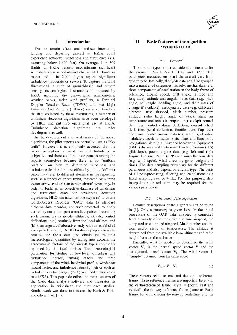
The increased accuracy in the estimate of altitude at lower altitudes due to the radio altimeter being used helps in reducing the covariance of the state vector not only at low altitudes but also at higher altitudes, due to the dynamic processes involved. This filtering-smoothing process works both ways, i.e. for a landing case as well as a take-off case. Only when applying the smoother this increase in accuracy can be obtained for the higher altitudes; with a filter only this would not have happened, or only to a much lesser degree. A typical example is given of the estimate of the inertial vertical velocity z , as well as its standard deviation

z taken from the covariance matrix Ni /P , as

function of time as it developed for a particular landing approach in Figure 1.

a) vertical velocity and std. dev.

b) altitude and ‘zdot’ std. dev.

Figure 1 Envelope of vertical velocity ‘zdot’, its std.dev. and altitude

As one can see the vertical velocity varies from +4 m/s (descent at 790 fpm) to near zero at t=250s, and finally back to zero again at the end (landing). The standard deviation in the estimate of the vertical velocity starts off at about 0.7 m/s, then drops quickly to 0.5 m/s, where it more or less stays constant at this value, and at the end it drops further to 0.2 m/s just before landing (i.e. from the moment the radio altimeter signal is being used in the calculated altitude, which is at 200 ft AGL or lower). This shows that the overall accuracy in the estimated vertical velocity, and hence wind component, is in the order of 0.5 m/s (1 Kt) or better, but it also shows that it is a dynamic process. Due to the fairly long times involved the filtered-smoothed covariance reaches steady-state values for most of the time.

II.4. Angle of attack calibration

One of the primary sources of information for the QAR data analysis is the calibrated angle-of-attack, obtained from the angle-of-attack vane (AOA-vane). There is a relationship between the AOA-vane and the “true” aerodynamic angle of attack α, which is used in

7

NLR-TP-2010-435

the calibration. This calibration, usually for a number of aircraft configurations (i.e. different flap settings), is normally not available, and has to be derived from the QAR data. The calibration equation generally is:

iFiAOAaiFaiAOAaoaic ..3.2.1 (4)

It is assumed there is a time lag ‘’ between the measured vane angle AOA and the actual calibrated

angle of attack ic due to QAR recording time delays,

pneumatic line time lags and all other sorts of factors that could introduce delays. In general the delay found varied between 0.25s and 1s. The time lag was found from the peak values in the cross-correlation between the measurement of AOA at time t and the computed inertial angle of attack at time t+. The calibration coefficients a0 – a3 are determined once per aircraft type through a multi-linear regression analysis.

II.5. Sideslip angle estimation

II.5.1 Original estimate A second aerodynamic parameter for calculating meteorological variables is the aerodynamic sideslip angle, usually denoted by β. In all the aircraft QAR data considered so far, there is no measurement of the sideslip angle, so an estimation process had been developed [20]. Principally it is derived from the original approximation that the lateral force on the aircraft comes from the tail fin due to the sideslip angle. The original sideslip angle was derived from the lateral acceleration Ay minus the bias in the lateral acceleration as:

m

ycSaV

m

finYyyA

fin2

21

(5)

Here the side force coefficient yc is linearized with

respect to β and the gradient approximated using slender airfoil theory applied to the tailfin as

73.5 where, ycycyc (6)

and it is based on the tailfin surface area Sfin. The resulting sideslip angle was then computed, correcting the lateral acceleration with the estimated bias y, during a flight according to

ycfinSaV

yyAm

221

(7)

II.5.2 Improved estimate of β In due course it was found that resulting sideslip angles sometimes reached fairly large and unrealistic values, of up to 10º-20º. To alleviate that effect a more thorough analysis was performed on the linearised yawing equation and the forces contributing to the side force Y. This equation plus more information is given in [19]. The first notion to make is that in Eq.(5) it was assumed that only the tailfin would contribute to the side force as result of a slip angle, however, the fuselage contribution can also be substantial. Thus it was decided to re-write Eq. (5) as:

m

fusYfinY

m

YyyA

(8)

Here the side force from the fuselage is estimated to be:

.22

1sin fusSaV

fusdcfusDfusY (9)

using the small-angle assumption. Combining the previous equations one can write for the improved estimate for :

fusdcfinS

fusSycfinSaV

yyAmimpr

221

(10)

Compared to Eq.(7) the coefficient in the denominator is no longer yc but is now

fusdcfinS

fusSyc , which can be substantially larger

than before, hence the sideslip angle will be much less. One could rewrite Eq. (10) as:

Kimpr (11))(a)

where the “gain” K (or correction coefficient) is:

1

1

1

yc

fusdc

tailfinS

fusSK

(11))(b)

However, how much less than 1.0 is not known, as the fuselage “side” area as well as the isolated fuselage drag coefficient are difficult to estimate accurately. At any rate, the inclusion of fuselage drag does give rise to the notion that a gain correction on the computed sideslip angle could be in order.

By also taking the (linearised) yawing equation of motion into consideration a methodology was developed in [6] to estimate the “corrective” gain value for each aircraft type, which came out in the order of

8

NLR-TP-2010-435

0.3-0.6. The result of this was that peak values for Turbulent Kinetic Energy ‘TKE’ and Eddy Dissipation Rate ‘EDR’, for example, much better matched one another, as the TKE calculation is sensitive and EDR is much less sensitive to the sideslip angle. The application of the corrective gain for sideslip is illustrated in the determination of winds and turbulence for a flight with a B777 aircraft, see the crosswind component in Figure 2. With the application of the corrective gain it is apparent that the variations in the crosswind component are reduced, although the general trend remains the same.

Figure 2 Crosswind component with (red, dashed)/ without (blue, solid) sideslip corrective gain for the B777 flight The reduction in the wind variation, viz. turbulence, brought about by the application of the corrective gain, also shows up in the Turbulent Kinetic Energy TKE plot, see Figure 3.

Figure 3 Turbulent kinetic energy with (red, dashed)/ without (blue, solid) sideslip corrective gain for the B777 flight

The TKE without the application of the gain correction reached peak values of 16 m2/s2, which corresponds to heavy turbulence [18]. With the corrective gain the peak TKE gets to about 5.5 m2/s2

only, which is a medium turbulence level [18]. The EDR1/3 is not affected very much by the corrective gain for sideslip, see Figure 4.

The EDR1/3 peaks to about 0.28 m2/3s-1, which corresponds to a light-to-moderate turbulence level. This is more consistent with the TKE profile with the application of sideslip correction.

K_beta=1 K_beta=0.551

0 50 100 150 200 250 300 350 400

TIME [S]

0.00

0.05

0.10

0.15

0.20

0.25

0.30

Ed

dy

Dis

sip

ati

on

Ra

te (

ED

R)1

/3

[m2

/3.s

-1]

Figure 4 Eddy dissipation rate with (red, dashed)/without (blue, solid) sideslip corrective gain for the B777 flight

II.6. Other parameters

II.6.1 TKE and windshear With the above processing, the three components of the wind are determined as per Eq. (1):

sin

sincos

coscos

:frame-E in the components itsin or

aVimpraVimpraV

Tbe

z

y

x

zwVwVwV

ba

Tbe

eea

ew

y

x

e

T

VTVVVV

With the wind vector known, the windshear parameters such as headwind change and windshear hazard can also be calculated. The windshear hazard factor ‘F’ is the time rate of change in total (kinetic plus potential) energy at time t due to wind changes and is calculated as follows (see [17], [20]):

a

waw V

ttt

gtF

kVeV

)()()(

1)( (12)

where the vector ae is the unit vector along the

airspeed vector and k is the unit vector along the vertical axis (positive “into” the earth). The definition is such that for a downdraft, i.e. positive component

zwV , the F-factor is negative as it implies a loss of

energy.

9

NLR-TP-2010-435

The turbulent kinetic energy is computed from the standard deviations in the 3 wind components

2/

2/

2)](,,)(,,[1

)(2,,

wTt

wTtdzyxwVzyxwV

wTtwvu

where the running mean value zyxwV

,, is computed

from:

2/

2/)(,,

1)(,,

wTt

wTtdzyxwV

wTtzyxwV

The turbulent kinetic energy TKE is then computed from

2222

1wvuTKE (13)

The “window” time interval Tw is specified by the program user. The calculation of EDR is a more complicated process, which will be described in chapter III. II.6.2 Wake vortex encounter event In fact the program WINDSTURB can do a lot more. The core of the program was programmed to be able to detect from the QAR data whether or not the aircraft had flown through a wake vortex encounter. Such an event is detected using the magnitude and signal-to-noise ratio of the computed vorticity (a vector quantity), which is the rotation in the airflow surrounding the aircraft. In order to be able to compute this parameter, an extensive list of additional parameters had to be recorded, e.g. aileron and spoiler deflections, angular rates, etc. Details of the algorithm are beyond the scope of this paper, and the reader is referred to [20]. The vorticity vector can eventually be expressed in earth axes as:

x

V

x

Vz

V

z

Vy

V

y

V

xy

zx

yz

ww

ww

ww

z

y

x

γ (14)

As a case in point, such an event was detected on one flight approaching HKIA. This flight was flown by an A320 on July 24th, 2005. A plot of runway cross-track versus runway along-track distance (km) from touchdown is given in Figure 5.

HDA 761; July 24th, 2005

35302520151050

RWY ALONG-TRACK DISTANCE [KM]

70

60

50

40

30

20

10

0

-10

RW

Y C

RO

SS

-TR

AC

K D

IST

AN

CE

[KM

]

WVE

Figure 5 Flight path where WVE occurred

It shows a segmented flight towards the airport, with interception of the computed final approach course of 251º true (253º magnetic) at about 25 km or 13 NM from the airport. The program corrected for the small track error that was present by introducing a bias of about 1 degree. The location where the wake vortex encounter (WVE) occurred is marked by the diamond symbol. The altitude at the moment of encounter was 1374 m (4507 ft).

The angle of attack profile during this flight is shown in Figure 6.

DISTANCE TO TOUCHDOWN [NM]

AN

GL

E O

F A

TT

AC

K [

DE

G]

0

2

4

6

8

10

02468101214161820

Figure 6 Angle of attack versus distance to touchdown As the figure shows, there is a spike in angle of attack at about 16 NM from touchdown, with a total AOA (Angle Of Attack) change of about 4º, which is due to the wake vortex encounter.

The fact that it was indeed a WVE is obvious when looking at the roll angle. The roll angle is shown in Figure 7.

10

NLR-TP-2010-435

DISTANCE TO TOUCHDOWN [NM]

BA

NK

AN

GLE

[D

EG

]

-25

-20

-15

-10

-5

0

121314151617181920

Figure 7 Roll vs distance to touchdown during wake vortex encounter At the same distance of 16 NM from touchdown, there is what looks like a roll reversal of about 10º magnitude, first in the sense of rolling back and then back to the bank angle in the turn it was supposed to have (i.e. -25º). The “correction” back to -25º is due to the autopilot, the upset from -25º to -11º was due to the airplane entering a wake vortex generated by a preceding aircraft. This roll angle upset of 10º is subjectively rated as “moderate” by all accounts, depending also on the altitude (above 2000 feet AGL) at which it occurs and the duration of the event.

A plot of the magnitude and signal-noise ratio of the vorticity in non-dimensional form (in the runway reference frame) is given in Figure 8.

02468101214161820

DISTANCE TO TOUCHDOWN [NM]

0

1

2

3

4

5

MA

GN

ITU

DE

OF

VO

RT

ICIT

Y [

-]

0

2

4

6

8

10

SIG

NA

L-N

OIS

E R

AT

IO [

-]

MAGNITUDE SIGNAL-NOISE RATIO

Figure 8 Vorticity vs distance to touchdown during wake vortex encounter

The signal-noise ratio peaks to well above 8.0 at 16 NM, where the vorticity magnitude itself peaks to just above 1.0. The signal-noise ratio turned out to be a good indicator to tell whether or not a WVE event occurred.

III. Calculation of eddy dissipation rate for turbulence studies

In the inertial sub-range, defined by the similarity hypothesis of Kolmogoroff [22] or Von Karman [21], the statistical properties of turbulence (e.g. standard deviation, kurtosis, etc.) depend only on , the eddy dissipation rate of turbulent kinetic energy. The eddy dissipation rate denotes the rate at which (at the smallest scales) well developed turbulent energy is converted into heat.

Traditional methods such as by MacCready [23], used to quantify the atmospheric turbulence during flight, depend on the measurement of aircraft unsteady movements (accelerations). According to MacCready [23], for a given aircraft type, speed and wing loading, the rms of the vertical accelerations g is linearly proportional to 1/3. This suggests using 1/3 (called EDR) instead of as the basic intensity parameter for atmospheric turbulence. The proportionality constant between g and 1/3 is a function of the aircraft response characteristics (aircraft type) and varies with altitude, aircraft weight, control settings and speed.

Some information on the role of aircraft dependent parameters is given by Bach and Wingrove [5]. The related problem of determining the aircraft movement in a given atmospheric turbulence field is discussed by Buck and Newman [9]. Together, these give an impression of the complex aerodynamic aspects involved in the derivation of the aircraft response factor, as needed when deriving the atmospheric turbulence from measured vertical aircraft accelerations.

The traditional method to quantify atmospheric turbulence has been through the measurement of vertical acceleration ‘g’. Because of its importance to monitor vertical gust loads, this parameter is usually also sampled at a higher sampling rate than other atmospheric parameters such as angle of attack. The next parameter that was derived from it in order to have an aircraft-type independent parameter was the Derived Equivalent Vertical Gust Velocity (DEVG), as defined by Sherman ([26] and [27]).

More recently EDR was also developed for use in AMDAR systems [2] and the implementation used is based on the vertical acceleration method of Cornman et al [16], which is based on the proportionality between g and 1/3 and therefore requires substantial aircraft-type dependent information. Detailed field comparisons between EDR and DEVG have been made by Stickland [29], showing a high correlation between peak EDR and DEVG for turbulence incidents. From this study Stickland also advised that the EDR method is to be preferred for classifying the atmospheric turbulence, because it is less aircraft dependent. The EDR algorithm was applied to NASA

11

NLR-TP-2010-435

flight tests with a B757 and a Convair and the analysis of these results led to an optimization of the algorithm, in particular on the choice of the frequency range to be used, as described in [24]-[25].

It should be mentioned that the current scheme applies typically for en-route conditions (i.e. altitude, airspeed and weight) of medium-sized transport aircraft. Further work is needed to come up with a suitable turbulence severity classification scheme for approach and take-off conditions.

Since 2001 a new EDR algorithm is under development at NCAR that is only based on the atmospheric wind components and thus should be less aircraft dependent. This method is based on the derivation of wind components in the earth fixed co-ordinate system. Inspired by the method to evaluate atmospheric wind components, as outlined by Bach ([4]-[5]), Cornman at NCAR [15] developed a method (called ‘Body Wind Algorithm’) to obtain the EDR values directly from the wind components. This method seems to offer advantages over the vertical acceleration algorithm and therefore is highly promoted in the US. Since 2006, following initial testing with the B757 aircraft of NASA, the method has been implemented in more than 100 aircraft of Southwest Airlines.

According to Cornman [14] in-situ turbulence data are potentially useful to:

Augment existing Pilot Incident REPorting (PIREP) data.

Provide near real-time state of the atmosphere to pilots, dispatchers, airlines and aviation meteorological services.

Provide a quantitative database for the verification of turbulence forecasting algorithms.

Provide input to turbulence diagnostic algorithms.

Provide a climatology of turbulence. Provide potentially direct input into

Numerical Weather Prediction (NWP) models.

Provide input to wake vortex decay transport and decay modeling.

Can be used to compute aircraft loads. For the specific situation at Hong Kong International

Airport (HKIA) the study of ambient atmospheric turbulence at and in the immediate surroundings of the airport as well as along the approach and departure routes is of utmost importance. As reported by Chan ([12]- [13]) this is currently partly based on LIDAR scanning and wind profiler information. The use of in-situ data could improve the turbulence prediction and warning, especially along the approach and departure routes. For this purpose HKO has installed an adapted version of the NLR EDR algorithm to process FDR

data from local airlines. The computation of EDR is based on the ‘Body Wind Algorithm’, as described by Cornman [15].

As derived from the first principle of turbulence, the calculation of EDR requires the solution of the power spectrum of the vertical wind component over a selected time window with a certain vertical mean velocity. A more practical method is to employ a running-mean standard deviation (sigma) calculation of the bandwidth-filtered vertical wind [7]:

)(05.1 3/22

3/21

3/2

3/1

aV

w

(15)

The vertical wind component

zwV is to be filtered with

a digital band-pass filter with cut-off frequencies f1 and f2 (with ω=2πf). Airspeed Va is passed through a low-pass filter in order to represent the average flying speed for the running time interval, and w is

computed as the running standard deviation (on the sliding time-window) of the band-pass-filtered vertical wind variations. A sensitivity study of EDR computation with respect to the input parameter values has been conducted [7]. It was found that, based on inspection of vertical wind spectra over the selected cases, there seems to be no need to employ a low-pass filter to the vertical wind signal. Only high-pass filtering would be required. The influence of the high-pass frequency on the evaluated EDR values appeared to be rather small. It is suggested to use f1 = 0.1-0.2 Hz and f2 = 2 Hz (the effective maximum detectable frequency in a 4 Hz sampled signal) in Eq.(15). The moving time window size of 10-20 seconds also appears to be a proper value. Other parameters that could be important for meteorological purposes are the static (or potential) air temperature, the temperature lapse rate, air density and the Richardson number, to name a few. If more specific parameters are required by the user then accommodations can be made to the software to output these quantities as well.

IV. Application examples

The first case is a significant windshear event that has been analyzed in [18]. An aircraft (B747-400) landed at HKIA from the west on 29 March 2005 and the pilot reported encountering windshear of +40 knots headwind gain during landing. From the wind speed computed from the QAR data, there is a wind change (increase) of ~12 m/s (24 knots) at about 2 nautical miles (NM) from touchdown (Figure 9).

12

NLR-TP-2010-435

Figure 9 Wind variation along the approach This wind change is smaller than the magnitude of windshear reported by the pilot. In order to reveal what has happened, the airspeed and ground speed of the aircraft are plotted together in Figure 10.

Figure 10 Airspeed and ground speed versus distance to touchdown for the B747 flight At 3 NM from touchdown, both the airspeed and the ground speed are almost the same. From 3 NM, the airspeed increases by about 20 m/s (40 knots). However, the ground speed increases also, but by about 10 m/s (20 knots) only. The raw data file indicated that at this point the aircraft was under control of autopilot C in COMMAND mode, but the Auto-throttles (AT) apparently had not been engaged (they were OFF for the entire duration of this segment of flight), so the pilot-flying must have manually controlled the speed with the throttles. This may be obvious from the rather irregular, step-like pattern of response of the throttle positions in Figure 11 (under autopilot control a much smoother, more continuous pattern would have emerged).

Figure 11 Throttle activity versus distance to touchdown for the B747 flight Therefore the pilot-reported “wind change of +40 knots” was actually an airspeed change of +40 knots due to a) a wind change of only 20 knots and b) a ground speed increase also of 20 knots because of pilot action. The second example shows the varying wind, turbulence and windshear variations for a flight in July 2005, a landing approach on runway 25 where a windshear alert could have been given. The FMS-stored windspeed and computed windspeed (filtered) for that flight are shown in Figure 12.

CPA 2039, July 2005 Hong-Kong

0246810121416

DISTANCE (NM)

0

2

4

6

8

10

12

14

16

WIN

D S

PE

ED

[M

/S]

FMS Computed + filtered

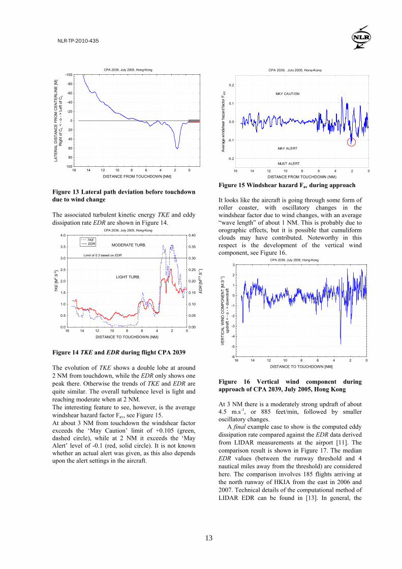
Figure 12 Wind speed (FMS, calculated) along approach of CPA 2039, July 2005, Hong Kong Notice the increase in windspeed at just before 2 NM from touchdown of about 6 m.s-1 or 12 kt. This gave rise to a drift from final track of about 60 m to the right, see Figure 13.

13

NLR-TP-2010-435

CPA 2039, July 2005, Hong-Kong

0246810121416

DISTANCE FROM TOUCHDOWN [NM]

-100

-80

-60

-40

-20

0

20

40

60

80

100

LA

TE

RA

L D

IST

AN

CE

FR

OM

CE

NT

ER

LIN

E [M

]R

igh

t of

CL <

- o

- >

Lef

t of

CL

Figure 13 Lateral path deviation before touchdown due to wind change The associated turbulent kinetic energy TKE and eddy dissipation rate EDR are shown in Figure 14.

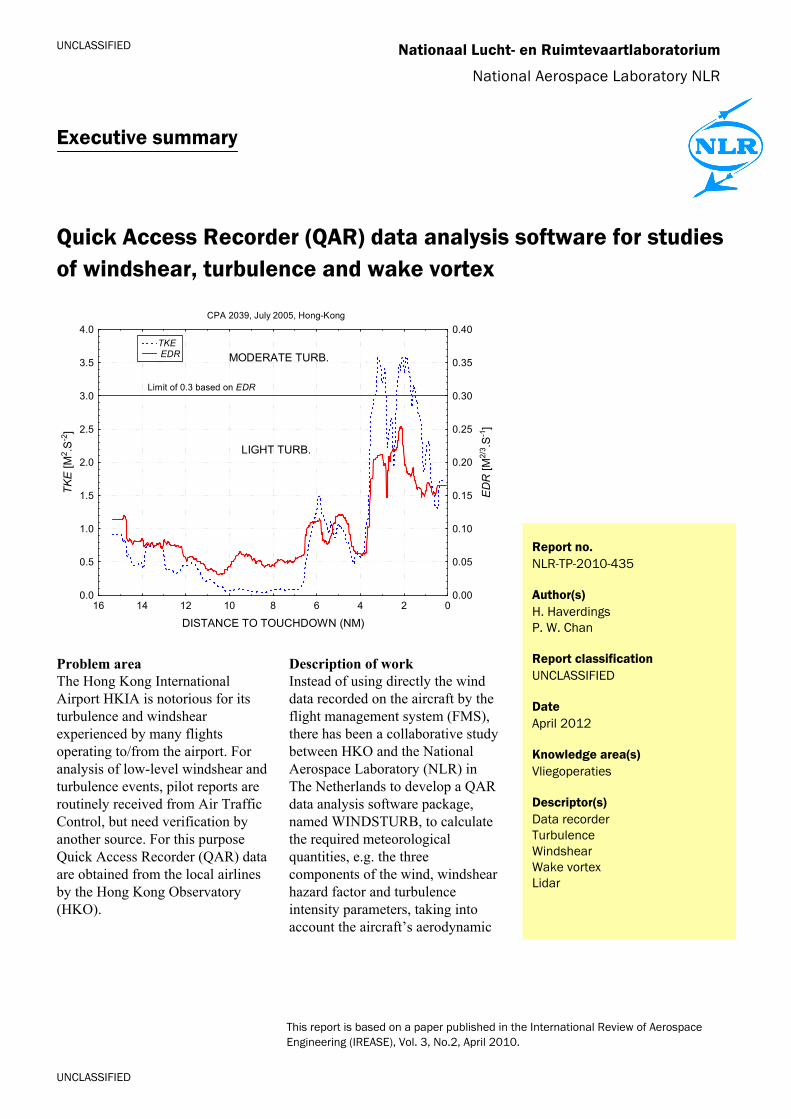
CPA 2039, July 2005, Hong-Kong

0246810121416

DISTANCE TO TOUCHDOWN (NM)

0.0

0.5

1.0

1.5

2.0

2.5

3.0

3.5

4.0

TK

E [

M2.S

-2]

0.00

0.05

0.10

0.15

0.20

0.25

0.30

0.35

0.40

ED

R [

M2

/3.S

-1]

TKE EDR

Limit of 0.3 based on EDR

LIGHT TURB.

MODERATE TURB.

Figure 14 TKE and EDR during flight CPA 2039 The evolution of TKE shows a double lobe at around 2 NM from touchdown, while the EDR only shows one peak there. Otherwise the trends of TKE and EDR are quite similar. The overall turbulence level is light and reaching moderate when at 2 NM. The interesting feature to see, however, is the average windshear hazard factor Fav, see Figure 15. At about 3 NM from touchdown the windshear factor exceeds the ‘May Caution’ limit of +0.105 (green, dashed circle), while at 2 NM it exceeds the ‘May Alert’ level of -0.1 (red, solid circle). It is not known whether an actual alert was given, as this also depends upon the alert settings in the aircraft.

CPA 2039, July 2005, Hong-Kong

0246810121416

DISTANCE FROM TOUCHDOWN (NM)

-0.2

-0.1

0.0

0.1

0.2

Ave

rage

win

dshe

ar h

azar

d fa

ctor

FA

V MAY CAUTION

MAY ALERT

MUST ALERT

Figure 15 Windshear hazard Fav during approach It looks like the aircraft is going through some form of roller coaster, with oscillatory changes in the windshear factor due to wind changes, with an average “wave length” of about 1 NM. This is probably due to orographic effects, but it is possible that cumuliform clouds may have contributed. Noteworthy in this respect is the development of the vertical wind component, see Figure 16.

CPA 2039, July 2005, Hong-Kong

0246810121416

DISTANCE TO TOUCHDOWN [NM]

-6

-5

-4

-3

-2

-1

0

1

2

3

VE

RT

ICA

L W

IND

CO

MP

ON

EN

T [

M.S

-1]

up

dra

ft <

- o

- >

do

wn

dra

ft

Figure 16 Vertical wind component during approach of CPA 2039, July 2005, Hong Kong At 3 NM there is a moderately strong updraft of about 4.5 m.s-1, or 885 feet/min, followed by smaller oscillatory changes.

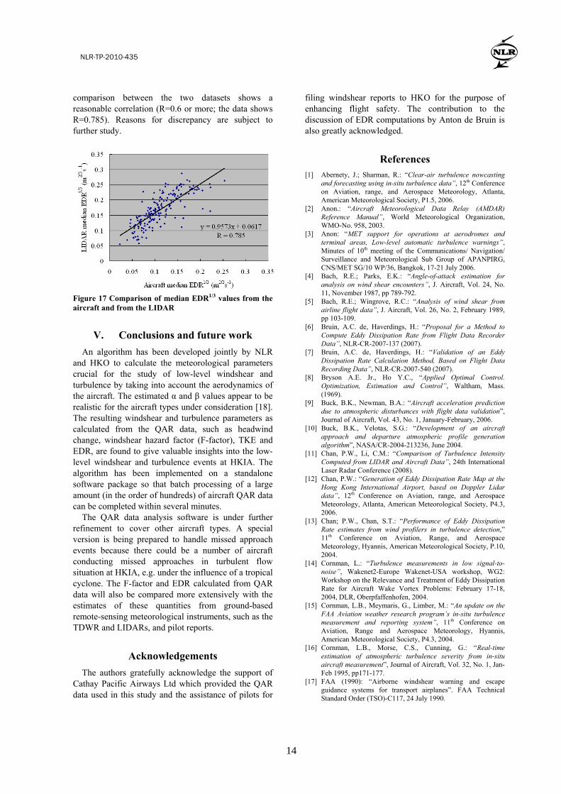
A final example case to show is the computed eddy dissipation rate compared against the EDR data derived from LIDAR measurements at the airport [11]. The comparison result is shown in Figure 17. The median EDR values (between the runway threshold and 4 nautical miles away from the threshold) are considered here. The comparison involves 185 flights arriving at the north runway of HKIA from the east in 2006 and 2007. Technical details of the computational method of LIDAR EDR can be found in [13]. In general, the

14

NLR-TP-2010-435

comparison between the two datasets shows a reasonable correlation (R=0.6 or more; the data shows R=0.785). Reasons for discrepancy are subject to further study.

Figure 17 Comparison of median EDR1/3 values from the aircraft and from the LIDAR

V. Conclusions and future work

An algorithm has been developed jointly by NLR and HKO to calculate the meteorological parameters crucial for the study of low-level windshear and turbulence by taking into account the aerodynamics of the aircraft. The estimated α and β values appear to be realistic for the aircraft types under consideration [18]. The resulting windshear and turbulence parameters as calculated from the QAR data, such as headwind change, windshear hazard factor (F-factor), TKE and EDR, are found to give valuable insights into the low-level windshear and turbulence events at HKIA. The algorithm has been implemented on a standalone software package so that batch processing of a large amount (in the order of hundreds) of aircraft QAR data can be completed within several minutes.

The QAR data analysis software is under further refinement to cover other aircraft types. A special version is being prepared to handle missed approach events because there could be a number of aircraft conducting missed approaches in turbulent flow situation at HKIA, e.g. under the influence of a tropical cyclone. The F-factor and EDR calculated from QAR data will also be compared more extensively with the estimates of these quantities from ground-based remote-sensing meteorological instruments, such as the TDWR and LIDARs, and pilot reports.

Acknowledgements

The authors gratefully acknowledge the support of Cathay Pacific Airways Ltd which provided the QAR data used in this study and the assistance of pilots for

filing windshear reports to HKO for the purpose of enhancing flight safety. The contribution to the discussion of EDR computations by Anton de Bruin is also greatly acknowledged.

References [1] Abernety, J.; Sharman, R.: “Clear-air turbulence nowcasting

and forecasting using in-situ turbulence data”, 12th Conference on Aviation, range, and Aerospace Meteorology, Atlanta, American Meteorological Society, P1.5, 2006.

[2] Anon.: “Aircraft Meteorological Data Relay (AMDAR) Reference Manual”, World Meteorological Organization, WMO-No. 958, 2003.

[3] Anon: “MET support for operations at aerodromes and terminal areas, Low-level automatic turbulence warnings”, Minutes of 10th meeting of the Communications/ Navigation/ Surveillance and Meteorological Sub Group of APANPIRG, CNS/MET SG/10 WP/36, Bangkok, 17-21 July 2006.

[4] Bach, R.E.; Parks, E.K.: “Angle-of-attack estimation for analysis on wind shear encounters”, J. Aircraft, Vol. 24, No. 11, November 1987, pp 789-792.

[5] Bach, R.E.; Wingrove, R.C.: “Analysis of wind shear from airline flight data”, J. Aircraft, Vol. 26, No. 2, February 1989, pp 103-109.

[6] Bruin, A.C. de, Haverdings, H.: “Proposal for a Method to Compute Eddy Dissipation Rate from Flight Data Recorder Data”, NLR-CR-2007-137 (2007).

[7] Bruin, A.C. de, Haverdings, H.: “Validation of an Eddy Dissipation Rate Calculation Method, Based on Flight Data Recording Data”, NLR-CR-2007-540 (2007).

[8] Bryson A.E. Jr., Ho Y.C., “Applied Optimal Control. Optimization, Estimation and Control”, Waltham, Mass. (1969).

[9] Buck, B.K., Newman, B.A.: “Aircraft acceleration prediction due to atmospheric disturbances with flight data validation”, Journal of Aircraft, Vol. 43, No. 1, January-February, 2006.

[10] Buck, B.K., Velotas, S.G.: “Development of an aircraft approach and departure atmospheric profile generation algorithm”, NASA/CR-2004-213236, June 2004.

[11] Chan, P.W., Li, C.M.: “Comparison of Turbulence Intensity Computed from LIDAR and Aircraft Data”, 24th International Laser Radar Conference (2008).

[12] Chan, P.W.: “Generation of Eddy Dissipation Rate Map at the Hong Kong International Airport, based on Doppler Lidar data”, 12th Conference on Aviation, range, and Aerospace Meteorology, Atlanta, American Meteorological Society, P4.3, 2006.

[13] Chan; P.W., Chan, S.T.: “Performance of Eddy Dissipation Rate estimates from wind profilers in turbulence detection,” 11th Conference on Aviation, Range, and Aerospace Meteorology, Hyannis, American Meteorological Society, P.10, 2004.

[14] Cornman, L.: “Turbulence measurements in low signal-to-noise”, Wakenet2-Europe Wakenet-USA workshop, WG2: Workshop on the Relevance and Treatment of Eddy Dissipation Rate for Aircraft Wake Vortex Problems: February 17-18, 2004, DLR, Oberpfaffenhofen, 2004.

[15] Cornman, L.B., Meymaris, G., Limber, M.: “An update on the FAA Aviation weather research program’s in-situ turbulence measurement and reporting system”, 11th Conference on Aviation, Range and Aerospace Meteorology, Hyannis, American Meteorological Society, P4.3, 2004.

[16] Cornman, L.B., Morse, C.S., Cunning, G.: “Real-time estimation of atmospheric turbulence severity from in-situ aircraft measurement”, Journal of Aircraft, Vol. 32, No. 1, Jan-Feb 1995, pp171-177.

[17] FAA (1990): “Airborne windshear warning and escape guidance systems for transport airplanes”. FAA Technical Standard Order (TSO)-C117, 24 July 1990.

15

NLR-TP-2010-435

[18] Haverdings, H.: “FDR Analysis of 3 Cases Delivered by Hong Kong Observatory”, NLR-CR-2006-114 (2006).

[19] Haverdings, H.: “Improved Sideslip Estimation for Application to FDR Data Delivered by the Hong Kong Observatory”, NLR-CR-2008-223 (2008).

[20] Haverdings, H.: “Updated Specification of the WINDGRAD Algorithm”, NLR-TR-2000-623 (2000).

[21] Karman, T. Von: “Progress in the statistical theory of turbulence”, Journal of marine Research, Vol. 7, No. 3, pp. 252-264, 1948.

[22] Kolmogoroff, A.N.: The local structure of turbulence in incompressible viscous fluids for larger Reynolds numbers, Dokalady ANSSSR, Moscow, 30, p.301, 1941.

[23] MacCready, P.B.: “Standardization of Gustiness Values from Aircraft”, Journal of Applied Meteorology, August 1964, pp 439-449.

[24] Robinson, P.A., Buck, B.K., Bowles, R.L., Boyd, D.L.B., Cornman, L.B.: “Optimization of the NCAR in situ turbulence measurement algorithm”, Aerospace Sciences Meeting and Exhibit, 38th, Reno, NV, Jan. 10-13, 2000, AIAA-2000-492.

[25] Robinson, P.A.: “Optimization of the NCAR in-situ turbulence algorithm”, presentation given at Weather Accident prediction Annual Project Overview, Hampton, VA, May 23-25, 2000.

[26] Sharman, R., Frehlich, R.: “Aircraft scale turbulence isotropy derived from measurements and simulations”, 41st Aerospace and Science Meeting and Exhibit, Jan 2003, Reno, AIAA-2003-0194.

[27] Sherman, D.J.: “Updated values of curve fit parameters for derived equivalent gust velocity”, Aeronautical Research Laboratories, Defence Science and Technology Organisation, Australia, 1997.

[28] Smalikho. I. N.: “Accuracy of the turbulent eddy dissipation rate from the temporal spectrum of wind velocity fluctuations”, Atmos. Oceanic Opt., Vol 10, No. 8, pp 559-563, 1997.

[29] Stickland, J. J.: “An assessment of two algorithms for automatic measurement and reporting of turbulence for commercial

public transport aircraft”, A report to the ICAO METLINKS/G. Observations and Engineering Branch, Bureau of Meteorology, Melbourne, 1998.

[30] Wingrove, R. C., Bach, R. E., Schultz, T. A.: “Analysis of severe atmospheric turbulences from airline flight records”, AGARD Flight mechanics Panel Symposium, Norway, May 1989 (also: NASA TM-102186, June 1989).

[31] Wingrove, R.C., Bach, R.E.: “Severe Turbulence and maneuvering from airline flight records”, Journal of Aircraft, Vol. 31, No. 4, July-August 1994, pp.753-760.

Authors’ information

Henk Haverdings was born on 22 April 1948. He is a research scientist at the National Aerospace Laboratory, NLR, Dept of Helicopters & Acoustics since 1973. He is employed in the area of rotorcraft flight mechanics, flying qualities and simulation. Since 1980, he has been involved in windshear research and FDR data analysis, including accident data related to windshear. Since 2004 he has developed software to analyse FDR data for the detection of the presence of wake vortex encounters.

P.W. Chan was born on 21 January 1970. He has been working at the Hong Kong Observatory as a scientific officer since 1994. His research interest includes meteorological instrumentation, windshear, turbulence, and numerical weather prediction model.