Bureau of Mineral Resources, Geology & Geophysics

DIVISION OF MARINE GEOSCIENCES & PETROLEUM GEOLOGY

Record 1989/27

BMR MARINE SURVEY 77TASMAN SEA:

EXPLANATORY NOTES TO ACCOMPANY RELEASE OFNON-SEISMIC DATA

by

A. Marks.

;pig"

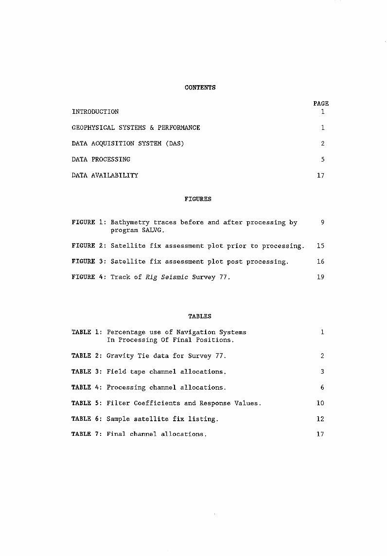
CONTENTS

PAGEINTRODUCTION^ 1

GEOPHYSICAL SYSTEMS & PERFORMANCE^ 1

DATA ACQUISITION SYSTEM (DAS)^ 2

DATA PROCESSING^ 5

DATA AVAILABILITY^ 17

FIGURES

FIGURE 1: Bathymetry traces before and after processing by^9program SALVO.

FIGURE 2: Satellite fix assessment plot prior to processing.^15

FIGURE 3: Satellite fix assessment plot post processing.^16

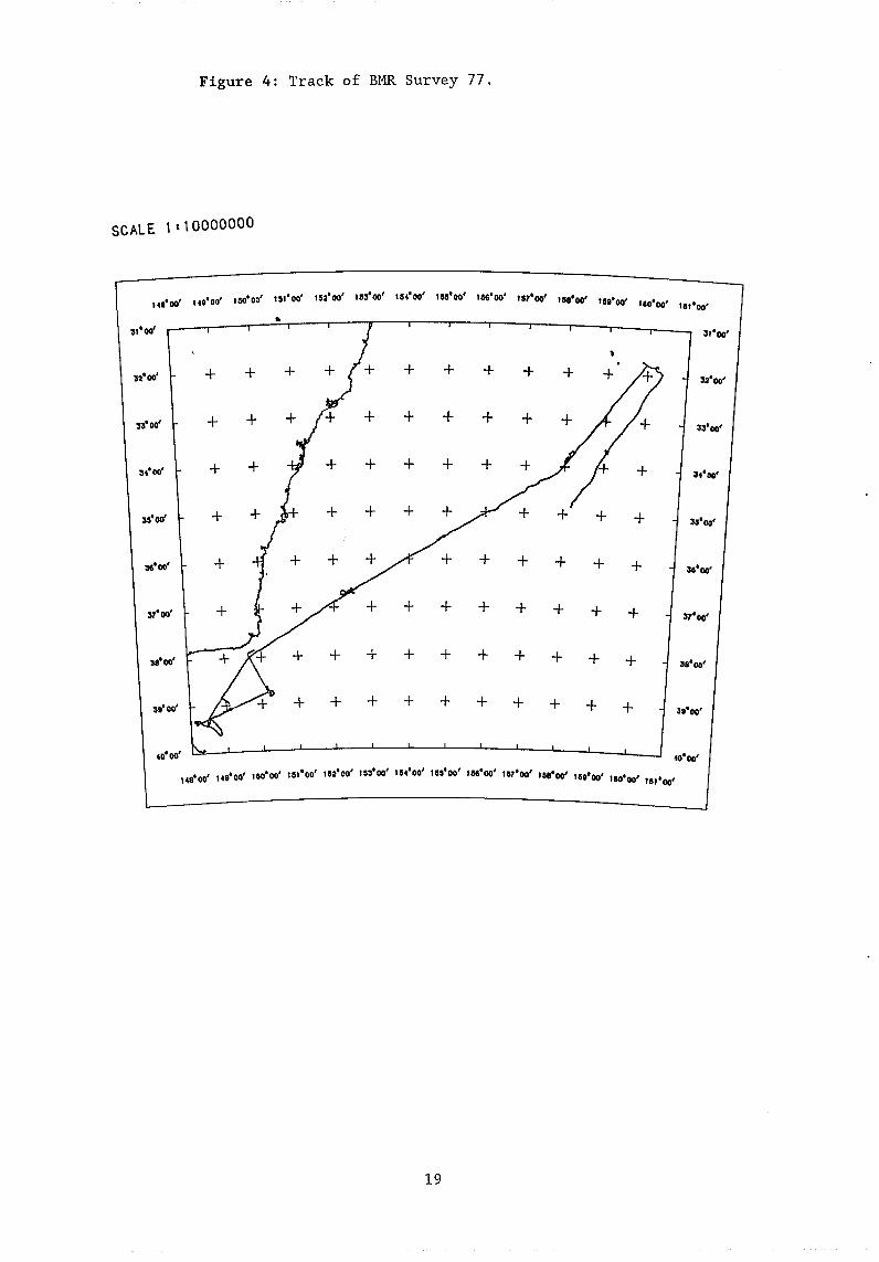
FIGURE 4: Track of Rig Seismic Survey 77.^ 19

TABLES

TABLE 1: Percentage use of Navigation Systems^ 1In Processing Of Final Positions.

TABLE 2: Gravity Tie data for Survey 77.^ 2

TABLE 3: Field tape channel allocations.^ 3

TABLE 4: Processing channel allocations.^ 6

TABLE 5: Filter Coefficients and Response Values.^10

TABLE 6: Sample satellite fix listing.^ 12

TABLE 7: Final channel allocations.^ 17

INTRODUCTION

The purpose of this report is to summarise the processing techniquesapplied to the non-seismic geophysical data collected on BMR Marine Survey77, in the Tasman Sea. Survey 77 was conducted between 10th February and15th March 1988 as part of project 9131.10.

GEOPHYSICAL SYSTEMS & PERFORMANCE

The following non-seismic geophysical systems were employed during Survey77

Navigation

Prime System: Magnavox MX1107RS dual-channel short-count TRANSIT satellitenavigator; ship speed from Magnavox 610D dual-axis sonar doppler andheading from Arma-Brown SGB 1000 gyro-compass.Secondary System: Magnavox MX1142 single-channel short-count TRANSITsatellite navigator; ship speed from Raytheon DSN-450 dual-axis sonardoppler and heading from a Robertson gyro-compass.Tertiary System: Magnavox T-Set Global Positioning System (GPS).Radio Navigation: Decca Hifix radio navigator using a set of three Hifixranges (channels) in psuedo-range mode transmitted from stations locatedon the coast.

Performance Comments: Both satellite navigators generally performedreliably. They were interfaced to the Data Acquisition System (DAS) andlatitude, longitude, course, speed (every 10 seconds) and all satellitefix details were transferred and recorded. T-Set data were good whenavailable, which was generally from 2200 to 0730 GMT.

Radio navigation data were received at distances up to 900 km from thetransmitting stations, however the data were very susceptible to noise atsuch distances. In addition atmospheric noise levels were high at nightand they were also high at dusk and dawn. Problems were experienced withthe drift levels of the atomic standards.

As processing of the long-range HIFIX navigation data was still at anexperimental stage, it has not been used to compute final positions.

Table 1: Percentage use of Navigation Systemsin processing of Final Positions.

System^Survey 77

Dead Reckoning^60%T-Set^ 40%

Both gyro-compasses performed satisfactorily for the entire survey, exceptfor a short period when they were inadvertently switched off.

Bathymetric Systems

Two Raytheon Deep-sea Bathymetric Systems, with a maximum power output of2 kW at 12 kHz and 2 kW at 3.5 kHz. These systems, designed in the early1970's, were of very sophisticated design for their day, providing in

1

addition to digital depths and various alarm flags, an automatic trackingfacility that should theoretically provide usable bathymetric data even inmarginal recording conditions.

Performance Comments: The general quality of the data varied from good toexcellent. The processing required to retrieve acceptable bathymetric datais described fully later in this report. Overall the data could bedescribed as very good. On this survey only the 12 kHz system was used.

Magnetics

Approximately 202 hours of magnetic data were recorded during Survey 77.

Performance Comments: After initial tuning, the Magnetometer systemperformed well until it was seriously damaged during deployment.

Gravity

Data were recorded from a Bodenseewerk KSS-31 marine gravity meter for theentire survey. Gravity ties were conducted in Sydney before Survey 77, andin Eden after the survey. Gravity tie information is provided in Table 2.

Performance Comments: The KSS-31 is a highly sophisticated single-axismarine gravity meter with extensive microprocessor control. Gravity datawere recorded for the entire survey with no problems.

TABLE 2: Gravity tie information for Survey 77

Place Date Time (GMT) KSS-31 value Corrected(mgal) (mgal)

Sydney 10.02.88 0333 -717.21 980389.99Eden 05.03.88 2326 -441.22 980387.03

Gravity meter drift - Sydney to Eden = 29.6 ums -2

DATA ACQUISITION SYSTEM (DAS)

The shipboard DAS is based on a Hewlett-Packard (HP) 1000 F-Series 16-bitminicomputer. Using the HP Real Time Executive operating system, data wererecorded either directly from the appropriate device through an RS-232Cinterface (gravity, Magnavox MX1107RS), or through a BMR-designed 16-bitdigital multiplexer (magnetics, bathymetry) and attached gyro-loginterface (for both sonar dopplers and gyro-compasses). After preliminaryprocessing, plotting on strip-chart recorders, and listing on a variety ofprinters, the data were recorded on 9-track, 1600 bpi, phase-encodedmagnetic tape in HP's 32-bit floating-point format.

Data were acquired and saved at a 10-second rate, regardless of ship speedand independently of the seismic acquisition system. The data were writtento tape in 1-minute (6 record) blocks with 80 channels of data beingrecorded. The channels that were recorded are listed in Table 3.

2

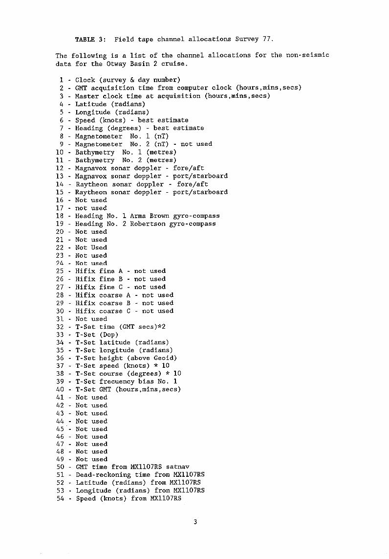
TABLE 3: Field tape channel allocations Survey 77.

The following is a list of the channel allocations for the non-seismicdata for the Otway Basin 2 cruise.

1 - Clock (survey & day number)2 - GMT acquisition time from computer clock (hours,mins,secs)3 - Master clock time at acquisition (hours,mins,secs)4 - Latitude (radians)5 - Longitude (radians)6 - Speed (knots) - best estimate7 - Heading (degrees) - best estimate8 - Magnetometer No. 1 (nT)9 - Magnetometer No. 2 (nT) - not used10 - Bathymetry No. 1 (metres)11 - Bathymetry No. 2 (metres)12 - Magnavox sonar doppler - fore/aft13 - Magnavox sonar doppler - port/starboard14 - Raytheon sonar doppler - fore/aft15 - Raytheon sonar doppler - port/starboard16 - Not used17 - not used18 - Heading No. 1 Aria Brown gyro-compass19 - Heading No. 2 Robertson gyro-compass20 - Not used21 - Not used22 - Not Used23 - Not used24 - Not used25 - Hifix fine A - not used26 - Hifix fine B - not used27 - Hifix fine C - not used28 - Hifix coarse A - not used29 - Hifix coarse B - not used30 - Hifix coarse C - not used31 - Not used32 - T-Set time (GMT secs)*233 - T-Set (Dop)34 - T-Set latitude (radians)35 - T-Set longitude (radians)36 - T-Set height (above Geoid)37 - T-Set speed (knots) * 1038 - T-Set course (degrees) * 1039 - T-Set frecuency bias No. 140 - T-Set GMT (hours,mins,secs)41 - Not used42 - Not used43 - Not used44 - Not used45 - Not used46 - Not used47 - Not used48 - Not used49 - Not used50 - GMT time from MX1107RS satnav51 - Dead-reckoning time from MX1107RS52 - Latitude (radians) from MX1107RS53 - Longitude (radians) from MX1107RS54 - Speed (knots) from MX1107RS

3

55 - Heading (degrees) from MX1107RS56 - Set (degrees) from MX1107RS57 - Drift (knots) from MX1107RS58 - Set/drift flag, 0 = No. 1 , 1 = auto from MX1107RS59 - GMT from MX1142 satnav60 - Dead-reckoning time from MX114261 - Latitude (radians) from MX114262 - Longitude (radians) from MX114263 - Speed (knots) from MX114264 - Heading (degrees) from MX114265 - Set (degrees) from MX114266 - Drift (knots) from MX114267 - Set/drift flag, 0 = No. 1 , 1 = auto from MX114268 - Vector speed Magnavox sonar dopplar69 - Vector speed Raytheon sonar doppler70 - Not used71 - Not used72 - Not used73 - Not used74 - Gravity ,(um.s -2 )*1075 - ACX (ms )*l000 roll76 - ACY (ms -2 )*1000 pitch77 - Sea state78 - Not used79 - Not used80 - Not used

DATA PROCESSING

The data were processed on a Hewlett-Packard 1000 F-Series minicomputerutilising similar hardware and the same operating system as the DAS. Theprocessing was applied in two phases, as follows:

Phase /: Transcription of field tapes; correction of time errors;production of raw data plots; bulk editing (principally deletion of baddata segments); retrieval of water depth data; minor editing; anti-aliasfiltering; computation of incremental latitudes and longitudes; productionof final check plots; final editing.

Phase 2: Resample 10-second data to 1-minute data; tying of the dead-reckoned (DR) track to the satellite fixes using a cubic-spline fittingtechnique to model ocean currents; assessment and deletion of poor qualitysatellite fixes; computation of final positions for each DR system;computation of final ship position from an appropriate mix of theavailable DR systems and the GPS system; computation of final Eotvos-corrected gravity, including a correction for gravity meter drift; finaldata editing (particularly gravity data during turns).

A brief summary of the processing steps follows

Phase 1

FCOPY: All field tapes were transcribed to processing tapes with severalfield tapes being combined into a single processing tape. Processing tapeswere separated at obvious breaks (such as recording system crashes) orafter about seven days recording. Time jumps (positive or negative) werereported for processing in the next phase.

FIXTM: Time jumps reported in FCOPY were corrected, either automatically,or with a file of manual time corrections. Data channels were re-ordered(Table 4) to simplify further processing.

VARPL: All raw data channels requiring processing were plotted as striprecords on a drum plotter. These plots were used to determine whereediting was required and as a first guide for the setting of filterparameters.

FTAPE: This program was used for a variety of tasks as follows:

(1) Removal of hardware/software flags in the bathymetric data. TheRaytheon echo-sounder system provides, in addition to digital bathymetry,'flags' indicating that the echo-sounder has lost track or that thedigitiser gate is searching for an echo. These flags were removed, asappropriate, and such values were replaced by the number 1.0E10 (10 raisedto the power 10), to indicate absent data.(2) 'Bulk' deletions were done of any large blocks of irretrievable datain particular channels.( 3 ) Automatic interpolations were done across data gaps of. up to 120seconds for selected data channels.

GMUL2: All raw gravity data were divided by 100 to reduce them tomilligals. All three speed logs (each of which outputs a fixed number of'clicks' per nautical mile) were reduced to give speeds in knots.

SALVG (Water depth recovery): Briefly stated, the problem of bathymetryrecovery is to fill in all the gaps left after the Raytheon hardware-

5

TABLE 4: Processing channel allocations Survey 77

The following is a list of the channel allocations used for processingthe non-seismic data for the Otway Basin 2 cruise

1 - Clock (survey & day number)2 - GMT acquisition time from computer clock (hours,mins,secs)3 - Master clock time at acquisition (hours,mins,secs)4 - Latitude (radians)5 - Longitude (radians)6 - Heading (degrees) - best estimate7 - Speed (knots) - best estimate8 - Bathymetry No. 1 (metres)9 - Bathymetry No. 2 (metres)10 - Magnetometer No. 1 (nT)11 - Magnetometer No. 2 (nT)12 - Magnetic gradient13 - Gravity (um.s -2 )*0.114 - Pitch acceleration (ms -2 )15 - Roll acceleration (ms -2 )16 - sea state filter number17 - Magnavox sonar doppler - fore/aft18 - Magnavox sonar doppler - port/starboard19 - Raytheon sonar doppler - fore/aft20 - Raytheon sonar doppler - port/starboard21 - T-Set Latitude22 - T-Set longitude23 - Arma-Brown gyro-compass (degrees)24 - Robertson gyro-compass (degrees)25 - Not used26 - Miniranger 1 not used27 - Miniranger 2 not used28 - Miniranger 3 not used29 - Miniranger 4 not used30 - Hifix (fine) A - not used31 - Hifix (fine) B - not used32 - Hifix (fine) C - not used33 - Hifix (coarse) A not used34 - Hifix (coarse) B not used35 - Hifix (coarse) C not used36 - 10-sec delta latitude - Magnavox S/D + Arma-Brown37 - 10-sec delta longitude - Magnavox S/D + Arma-Brown38 - 10-sec delta latitude - Magnavox S/D + Robertson39 - 10-sec delta longitude - Magnavox S/D + Robertson40 - 10-sec delta latitude - Raytheon S/D + Arma-Brown41 - 10-sec delta longitude - Raytheon S/D + Arma-Brown42 - 60-sec delta latitude - Magnavox S/D + Arma-Brown43 - 60-sec delta longitude - Magnavox S/D + Arma-brown44 - 60-sec delta latitude - Magnavox S/D + Robertson45 - 60-sec delta longitude - Magnavox S/D + Robertson46 - 60-sec delta latitude - Raytheon S/D + Arma-Brown47 - 60-sec delta longitude - Raytheon S/D + Arma-Brown48-55 - Not used56^- Not used57^- Final Bathymetry (metres)58^- Final Magnetometer No. 1 (nT)59^- Final Magnetometer No. 2 (nT) - not used60 - Not used61 - Not used

6

62 - Final Gravity (um.s -2 )*0.163 - Final Latitude (radians)64 - Final Longitude (radians)

7

software flags were removed and to discriminate against the badbathymetric values that still remain.

To accomplish this, a file was first created of manually digitised waterdepths at selected points. This file was then read in conjunction with theprocessing data file. SALVG then performs a straight line interpolationbetween adjacent tie points and compares the interpolated depth with the10-second digital depth. If the difference is less than a user-specifiedthreshold, then the digital depth is accepted and is used to replace theprevious first tie point. If the difference is greater than the threshold,then the 10-second digital depth is replaced by the interpolated depth. Inthis way, the program tracks along the acceptable water depths, providingthe threshold is small enough to reject bad data and large enough toaccept the good data. In the case of the digital data being totallyunacceptable, as during poor sea conditions, the threshold was set to avery small number (0.01 m) and the process became one of simple linearinterpolation between adjacent tie points. In practice, the intervalbetween manually digitised tie points varied from several hours in thecase of good digital 10-second data, to several minutes in the case ofpoor 10-second data or a very rugged seabed.

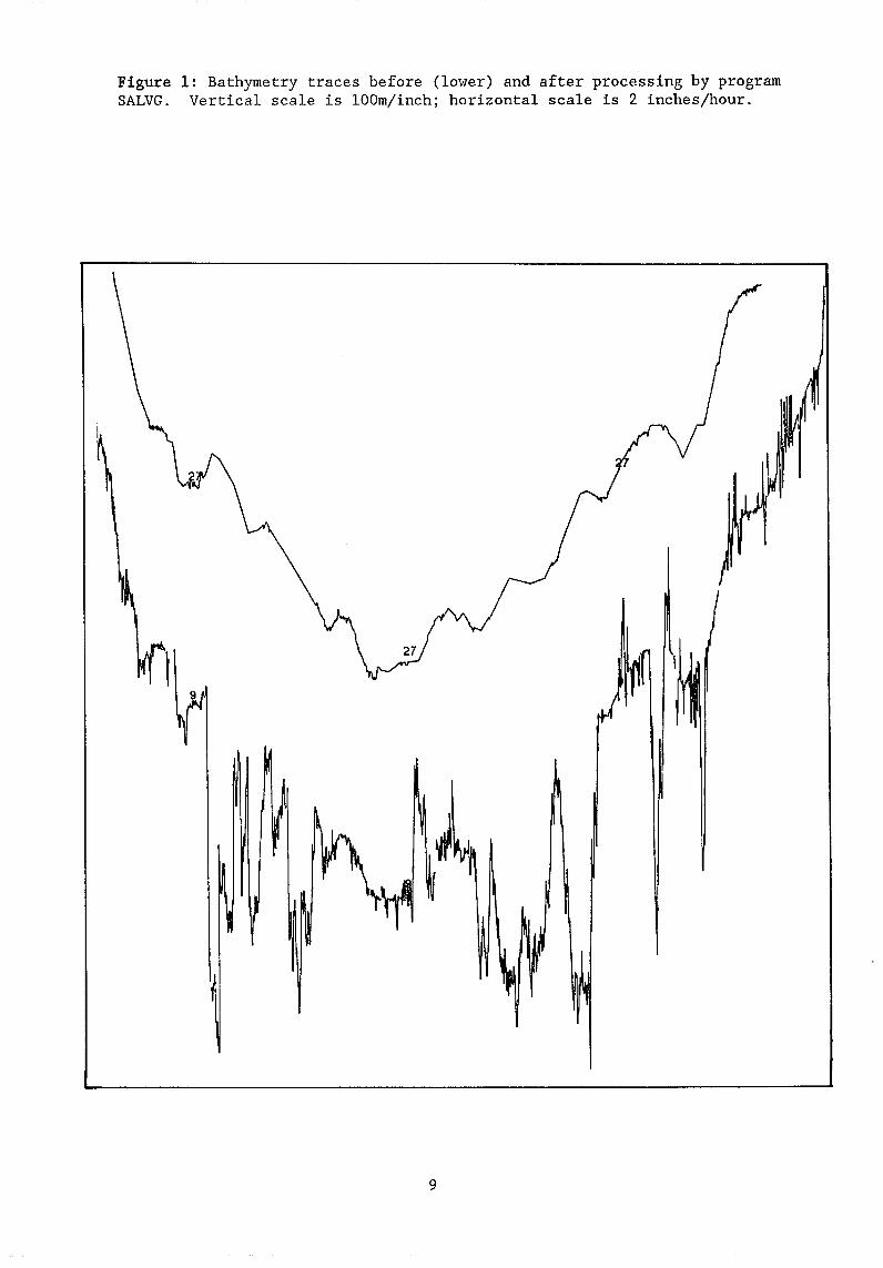
The success of this process, which is routinely applied to all Rig Seismicbathymetric data, can be seen in the following 'before and after' plots ofFigure 1.

FDATA: The magnetic, gravity and velocity data were filtered using asophisticated form of the median filter, a highly successful spikedeletion tool. Such a filter is essential for magnetic data, which issusceptible to spikes arising from either poor tuning of the magnetometeror from electrical interference. A filter threshold of 7.0 nt was usedwith a filter window length of 13 samples for magnetic data. A thresholdof 1 knot with a window length of 13 samples was used for the velocitydata.

EDATA: This is a utility program used for the manual editing of problemareas that are not amenable to filtering or automatic editing.

MUFF: This program was used to anti-alias filter certain data channelsprior to resampling to 60-seconds for Phase 2 processing. The channelsfiltered were magnetics, gravity and velocities. For the magnetic andgravity data the filter used was a SINC function with a filter period of180 seconds. For the velocities a SINC function with a period of 60seconds was used.The filter coefficients and the approximate responses toa sine wave are given in Table 5.

DELTA: Incremental (delta) latitude/longitudes were produced every 10seconds by combining the ship speed with the headings from the Arma-Brownand Robertson gyro-compasses. This effectively gave two distinct dead-reckoning (DR) systems.

INTEG: The filtered incremental latitude/longitudes were re-integratedover running 60-second intervals. These 60-second incremental distanceswere then used in the Phase 2 processing to compute the DR vector overeach satellite fix interval.

VARPL/EDATA: As the final stage of the Phase 1 processing, all processedchannels were plotted again as 'strip' plots with program VARPL. ProgramEDATA was then used to correct any minor residual data problems.

8

Figure 1: Bathymetry traces before (lower) and after processing by programSALVG. Vertical scale is 100m/inch; horizontal scale is 2 inches/hour.

9

TABLE 5:Filter coefficients and approximate response of filter to sinewave for magnetics smoothing filter.

SMOOTH FILTER^1 PUTS CHANNEL 11 INTO 11

FILTER CUT-OFF AT 3.RD ZERO

SAMPLING INTERVAL IN SECONDS 10.0

PERIOD OF FILTER IN SECONDS 180.0

APPROXIMATE RESPONSE OF FILTER TO SINE WAVE

NUMBER OF POINTS IN FILTER 53

FILTER COEFFICIENTS AS FOLLOWS.000 .001 .002 .003 .004 .004 .004 .003 -.000 -.004

-.008 -.012 -.015 -.018 -.018 -.015 -.009 .000 .012 .027

.043 .060 .076 .091 .102 .109 .111 .109 .102 .091

.076 .060 .043 .027 .012 .000 -.009 .015 -.018 -.018

-.015 -.012 -.008 -.004 -.000 .003 .004 .004 .004 .003

.002 .001 .000

FRACTION PERIOD RESPONSE db

.500 90.0 .00108 -59.3

.518 93.2 .00442 -47.1

.536 96.5 .00672 -43.5

.555 99.9 .00672 -43.5

.574 103.4 .00380 -48.4

.595 107.0 -.00178 -55.0

.616 110.8 -.00884 -41.1

.637 114.7 -.01548 -36.2

.660 118.8 -.01934 -34.3

.683 122.9 -.01804 -34.9

.707 127.3 -.00946 -10.5

.732 131.8 .00793 -42.0

.758 136.4 .03500 -29.1

.785 141.2 .07183 -22.9

.812 146.2 .11784 -18.6

.841 151.4 .17184 -15.3

.871 156.7 .23226 -12.7

.901 162.2 .29728 -10.5

.933 167.9 .36499 -8.8

.966 173.9 .43355 -7.31.000 180.0 .50127 -6.0

1.035 186.3 .56672 -4.91.072 192.9 .62872 -4.0

1.110 199.7 .68641 -3.31.149 206.8 .73918 -2.6

1.189 214.1 .78669 -2.1

1.231 221.6 .82882 -1.6

1.275 229.4 .86564 -1.31.320 237.5 .89735 -.9

1.366 245.9 .92426 -.7

1.414 254.6 .94676 -.5

1.464 263.5 .96527 -.3

1.516 272.8 .98024 -.2

1.569 282.5 .99210 -.11.625 292.4 1.00129 .0

1.682 302.7 1.00821 .11.741 313.4 1.01322 .1

1.803 324.5 1.01665 .11.866 335.9 1.01881 .2

1.932 347.7 1.01994 .2

2.000 360.0 1.02028 .2

10

PHASE 2

Phase 2 processing encompasses the following tasks:

1. Re-formatting and production of assessment listings of satellitefixes.

2. Resampling Phase 1 data.

3. Assessment of satellite fixes and deletion of those considereddubious or unacceptable.

4. Constrainment of DR track to remaining satellite fixes^andcomputation of 1-minute positions for each DR system.

5. Selection of a suitable mix of navigation systems to produce finalpositions.

6. Application of Eotvos and drift corrections to gravity data andconversion to absolute values.

7. Final plots and editing as necessary.

In rather more detail, the programs applied were as follows -

RESAF: Re-format the ASCII parameter file of satellite fixes and adjusteach fix to the nearest whole minute of survey time using the ship speedand heading applying at that time in the Phase 1 data file.

FIXES: Produce a listing of the satellite fixes for assessment purposes(Table 6).

RESAM: Concatenate the Phase 1 data files, as appropriate, and resample toproduce 1-minute data.

SAT12: Two passes of this program are required for each round of satellitefix assessment. During each pass, a number of options are called, asfollows:

Pass 1

a. SATEL - reads in the file of satellite fixes and stores them inmemory. Any fix intervals with dubious speeds (too low or too high) orany intervals that are very short (<15 minutes) or very long (>120minutes) are flagged in the output listing.

b. DRNAV - uses the incremental latitude/longitudes stored on the Phase1 file and the satellite fix information to compute the DR path (or DRvector) for each satellite fix interval. This is saved as an ASCIIparameter file.

c. CALNV - reads the DR file created by DRNAV and computes the ratio ofthe average DR velocity to the velocity computed from successivesatellite fixes. This is done for each DR system used, and the resultsare listed.

d. CALPL - produces a line printer plot of the velocity ratios for eachsatellite fix interval.

11

TABLE 6:

Sample listing of satellite fix parameters produced by program FIXES.

Column headings as follows:

FIX - satellite fix number within file.FIX TIME - computed time of fix in format SS DDD.HHMMSS,where SSis the survey number (67), DDD is the Julian day number in1987, and HHMMSS is the GMT time.LAT,LONG - Latitude & longitude of fix in degrees & Decimal minutes.SYSTEM - Magnavox 1107 or 1142, or dummy fix (DFIX).SAT - satellite number; OK - accepted (Y) or rejected (N) on-board.ELEV - maximum eTtvation of satellite (degrees).COUNT - number of doppler counts recieved.ITER - number of iterations required to compute fix.GEOM - geometry of pass.ERROR - amount of shipboard update (n.miles).DIR - direction of shipboard update (degrees).SLT,SLN - standard deviation of latitude & longitude (metres).CODE - error code if fix not accepted by sat nay.COURSE,SPEED - vessel's course and speed at time of fix.

FIY FIX TINE LAT !OM SYSTEN SAT 00 ELEV COUNT 11E9 SE0N E9988 PIP SLI 86N CDPE tOORSF 9E5E0

51 77.049.000900 33 26.830 159 13.312 1107 200 I 28 28 3 St 3.93 303 0 0 66.7 1.852 77.049.003400 13 25.43E1 159 14,432 1107 330 y 14 19 5 SE .77 315 0 0 71.8 3.753 77.049.005200 33 24.939 159 14.600 1107 500 Y 12 25 5 SO .89 267 0 0 70.7 3.854 77.049.011000 33 24.041 159 15.352 1107 110 1 14 25 3 SO .53 313 0 0 70.8 3.9

55 77.049.011000 33 22.903 154 16.277 1107 245 Y 21 29 3 HE .70 3 1 8 0 0 75.53 4 •056 77.049.015300 33 21.746 159 17.361 1107 200 Y 37 32 3 SO .74 305 0 0

774: 457 77.009.022000 33 20.193 159 17.939 1107 110 14 9,0 31 3 so 3.60 297 0 Si 1 8 4...1;58 77.049.03 1 800 33 17.087 159 22.600 1107 290 1 58 17 3 NO 2.26 331 0 0

1

5 9 77.049.041000 33 14.777 159 24. 4 22 1107 450 Y 31 33 1 HE 2.07 242 0 0 71.1 4.5

60 77.049•051400 33 11.217 159 27.545 1107 240 Y 16 28 3 HE 1.07 307 0 0 79.7 4.2

61 77.049.055900 33 8.459 159 29.602 1107 440 Y 38 35 3 NO .67 337 0 0 55,5 4.0

62 77.049.070300 11 5.013 159 32.521 1107 240 1.1 77 19 3 NU .56 300 0 0 1^• 44.0 4.1

61 77.0 4 9.0 04 900 32 5 8 .55 0 1 5 0 76.71 5 1107 7 4 0 I 15 25 7 NU 2.45 274 0 0 40,P. 45.2

64 27.544,503505 3? 55,545 559 41.575 1107 500 1 56 14 2 NE .86 231 0 0 41.3 3.9

65 77.049.111200 32 53,159 159 4 1.775 11 0 7 200 0 7 19 NE .19 235 0 0 2 39.3 4.2

66 77.049.121900 32 49.7 9 1 159 46.451 110? 500 Y 22 29 3 NO .90 235 0 0 29.8 4.0

67 77.049.125000 32 47.732 159 45.484 1107 200 N 53 26 6 HE .57 125 0 0 1 29.0 4.1

68 77.049.132500 32 46.187 159 49.936 1102 3 9 0 7 21 10 2 .20 112 0 0 24.5 4.1

69 2 7.049.131600 12 45.761 15 9 49.375 1153 130 y 50 29 3 HE .54,221 0 0 24.7 4.0

70 77.049.144200 32 42.050 159 51.094 1102 200 14 9 20 5 NV .62 217 0 0 1 27.5 3.571 77.049.151400 32 40.2 1 9 159 52.006 110 7 290 1 55 15 3 Sli .14 157 0 0 23.5 1.5

72 77.049.161500 32 16.316 15 9 53.7 4 0 1107 400 1 40 35 3 SE .36 263 0 0 23.5 3.9

73 77.049.171600 32 32.932 159 55.59 4 110 7 240 y 16 25 3 sE .61 269 0 0 17.2 4.2

7475

77.0 4 9. 1 8070077.0 4 9.190 4 00

3212

10.09226.8 9 6

15 9

15 9

57.40059. 4 77

11071107

48 0

241)1N

1075

3437

22

St!54

.68

.85261275

00

00 1

78.83b.7

4 .24 .1

76 77.0 4 9.207 00 32 20.742 1 60 4.111 111.17 500 N 7 20 1 SE 2. 4 0 290 0 0 1 4 ,:,.5 4.1

77 77.0 4 9.2233 0 0 32 15.6 4 0 160 9.084 1167 110 y 35 29 1:1_ 4 .16; r9.5

0 0

7E 27.049.225900 12 14.537 160 9.65 9 110 7 200 N 4 17 A 5 0 0 1-11?.1.? i ,..i79 77.050.002 0 00 12 11.'247, 1 140 13.61 7 11 1,7 1111 'f 12 1 0 3 SU 3.56 272 0 0

50 12 1 0.072 160 1 4 ,120 11 0 2 200 1 66 20 7 SE .55 26 7 6 0 43^1) 4 . 5

Si 32 7 .P. 1 5 160 1 4.1 71 5 1 0 7 1 70 ' 47 74 3 55 .5, 209 0 0 ',,P.,. 4.7

9283

77.050.02290077.050. 031600

3232

5. 4 5 1

1 .6221 601 60

10.1 7 520.615

11 4 25 107

200110

Y7

14

2129

28 SO 1 991.0 (;., 11 87 :11

024-.72.P1.. 11.1,

8 4 11 5 9 •753 160 21.596 1107 4 50 1 21 31 3 NE .29 224 0 0 24.5 4 ,3

05 77.05 1..0 0 7000 31 57.722 5 60 2 1 .975 1102 290 1 35 26 4 No .19 252 0 6 3517 3.111,1, 77711811283455..647S67711811283455. 31 56.526 160 2 1 ,400 11,)7 246 N 7 21 4 54 .24 72 0 0 1 ,1,)^5 1.5

87 77 .050• 6 c76 0 0 7 5 55.418 1 60 19.641 11 02 48 0 1 50 36 3 81.1 .21 50 0 0 312.2 .8Bs 77,056.11.2065 35 55.167 160 19.237 1107 240 y 47 34 2 NS .24 280 0 0 144.8 .0go 77.4)5(!.47g441( .46 11 54.15 146 15,410 1157 240 '4 19 25 3 NU .29 337 0 0 .11

9 0 7 7 .5;0.0 ,4 0fifi 1 5 51.5344 1 60 57 .42 53 1107 110 Y 15 25 3 HE .65 266 0 0 725.7

91 77.050.100E 00 31 53.575 160 17,303 1107 500 y Al 36 3 HE .10 294 0 0

9 2 77.050.1 149 00 3 1 5 4 .272 1 60 1 6.536 1107 200 1 21 19 3 NE .67 241 A 0 2,-,59 -.2

12

Pass 2

a. CFACT - uses the DR file and a user-created file of calibrationfactor intervals to compute velocity calibration factors for each DRsystem.

b. APROX - uses the calibration factors computed in CFACT and the DRfile to produce an approximately calibrated DR file.

c. ASSES - uses the approximately calibrated DR file created by APROXto produce a line printer plot of the current and summed error vectorsat and between satellite fixes. The plot is produced at a 10-minutesample interval.

The basis of the processing is that option 'ASSES' takes the summedlatitude and longitude error vectors at each fix (le a running sum of theDR position to satellite fix position vectors at the time of each fix) anduses a piece-wise cubic polynomial curve-fitting function (the Akimaspline) to compute error vectors at all times between satellite fixes. Itis assumed that the ensuing smooth variation of the error vector is due toocean currents, winds, etc. Poor quality fixes will produce unrealisticor large and variable ocean currents. At each round of assessment (andusually at least three rounds are required for each file) the satellitefixes are checked wherever the summed error and current vectors suggest aproblem, and those fixes of poor quality are deleted for the next programrun. The effect of this process can be seen in the example in Figures 2and 3.

SAT3: uses the final file of satellite fixes and the DR data to producefinal positions for each DR system. This program again uses the Akimaspline to compute the assumed currents acting at all times betweensatellite fixes and applies those currents to the DR data to computepositions.

FINAV: performs the following functions -

a. Computes final 1-minute positions based on a 'mix' of DR systems andthe Global Positioning System acording to a file specified by the user.

b. The gravity data (which were in mgals relative to an arbitrarydatum) were converted to absolute values relative to ISOGAL 84,corrected for meter drift and had Eotvos corrections applied; no tidalcorrections have been applied.

VARPL/EDATA/FIXTM/MUFF: As a final check, the Phase 2 positions, waterdepths, magnetic, and gravity data were plotted and editing applied asnecessary. The data was then re-blocked using program FIXTM to 8 channelsx 60 records per block (1-hour blocks); the final channel allocationsare shown in Table 7. Final editing involved the removal of gravityspikes at turns using EDATA and further filtering of sea noise in thegravity using MUFF with a filter of 15-minute period.

Figures 2 & 3 (following pages). Satellite fix assessment plots for apart of Survey 77. 10-minute time (DD.HHMM) along bottom of plot. Thesatellite fixes indicated by vertical row of dashes (eg at 058.1050).traces on plot are as follows:

N & E - north and east currents for DR system 1.1 & 2 - north and east summed error vectors for DR system 1.

13

Y & X - north and east currents for DR system 2.3 & 4 - north & east summed error vectors for DR system 2.

-^t:%1 Cl

,^:..., ,:•.:^ ••

I^.7:^:^ 1^:^••^I

Cli---, ,..., ......: ,., r-t '..., ....-1 "I r--i "1 , . , , .-1 ....4 t--; , ., ', , :--. r

-; 1- ' , '-: :-.1 "-I , , , .-4 .-i •-... , "4

.^., ..^....

7..-: a)^ CA C'.: Cj Cj 1n ZD 2:., ZD !

,3^!^ ........ : ■^L

- ..:) -:-J-

••^ 1^ i

! i^ !^1 nmi or I kn!

,

i

C....^!^I!^i^i

("I C%! CI l'j i^i^<I^

Ii^

...^.1

CJ^i^1^1

^

-^-

Figure 2:Satellite fix assessment plot.

1-q I-I ,..-.1 1-1 "4 1-1 I.-I ,1 ,i I, "1 ,1 I-1 ....1 I,^,

i^ i^•^ 1

1^ 1^1^ 1^1^1^ i

1

i^I^ i

.^;^1

1^ 1^!^ 1^ 1

;^ 1^1^t,^!^1

r

t^i

a^I

I^a^'

^

I^ '.^I^L -.1 1... - I L -I lari Iii.

^

I^1^L.:. Ln^i

^

i^!.^,...n Ln Ln i.^Ll Ln Ll Ln^I !

^

.....^..... v , Ln^ ..^',^--. •

71.!^r)

CA^C)I")^C3

DJ

Ci^ii

LnCA^2.i1

Z. C. Z. C. 0 C. an C. 00 0 0 0 0 0.^0^0 0- 0 000 0-^C., 0- C. ..

C.^U-1 ,— 0 an ,4 cJ^ CC^ CC ,422);".1^0,4^2.)

:7, CC CD^cn^'1^,1 ,1 .7..1 :A^=A^CA^r.1^ L, _n

.^.^.^.^.^ .^.^ .^ .

... C. 0-0 C. CJ C. C. 00 C. CO Z C. 00 0an CD Z. C. C. C. an an an C. 47 C.^43 C. an an 4.

1:1 11^Ln 1.1 Ll Lq^Ll^Ln L11.1 Ln 1.71^ 1.1 41 Ln Ln Ll 1,,^Ll

15

hi 7-i hi hi hi ry FY 0:^hi I hi ty hi ,y^!,^iy^hi hi hi ,Y^,i^ hi

•

!

1 7 -I ;":;II^l'•".

• -

.^•

1, •

,

Pl

•.•It 0.•-•,• •';'•^t!"..^-7..• It s-^C.; '"".'

.•0 ••7^„.4 ^v. ,i^ ,V

ItO It It It :•-'s It It It It Ito It It It It It It It It It It It It It It It It 0.,. 0.

1.1^!..10^:it V'^t.1 :0 LP^irt^Lrt.^1..-1^L.0^1.0 tit Ir!

--;

I^•-.0'^ C...! C.JI '^-:";^ 1..'..t

I •!-.1 .0^ C5i c . .1',II^1^ r...1

I^I^ CIJ!^ C.i !..". ..1

' .I•^—

•

• •^ 1

':

:^I^7. -.2^ :.•-■ 72 • !:•.j

Figure 3:Satellite fix assessment plot after removal of bad satellite

fixes at 050.1150 and 050.1320

16

TABLE 7:

Final channel allocations.

Channel number^Contents

1^Time (SS.DDD)2^Time (.HHMMSS)3^Latitude (radians)4^Longitude (radians), relative to 100 0 E5^Water depth (meters)6^Gravity (um.s -2 )*0.17^Total magnetic field (nT)8^Not used

DATA AVAILABILITY

The Tasman Sea non-seismic data is available in two forms:

a. Magnetic Tape - 9-track, 1600 bpi, phase-encoded, as either- ASCII records, 80 characters per record, 10xl-minute records perblock, or- Hewlett-Packard 32-bit floating point, 8 channels, 60x1-minuterecords per block.

b. Analogue Displays - on paper and film.

Lambert's Conformal projection maps at a scale of 1:1000000:- Cruise track charts- Profile maps of bathymetry, free-air anomaly and magnetic anomalies- Posted value maps of bathymetry, observed gravity, total magneticfield and magnetic anomalies

Enquiries concerning the data should be addressed to:

Chief ScientistDivision of Marine Geosciences & Petroleum GeologyBureau of Mineral ResourcesPO Box 378Canberra ACT 2601Australia

17

SURVEY 77, TASMAN SEA, MAPS PRODUCED

Track Maps

1:1000000 Sheet Name

SH57SYDNEY (SI56)SI57MELBOURNE (SJ55)BODALLA (SJ56)

Profile Maps

Bathymetric ProfilesFree-Air Anomaly ProfilesMagnetic Anomaly Profiles

Post Maps

Bathymetric valuesObserved Gravity ValuesTotal Magnetic Field ValuesMagnetic Anomaly Values

Sheet Nos. Product No.

^

1-5^

M-77M0001P

^

2-5^

M-77M0002P

^

3-5^

M-77M0003P

^

4-5^

M-77M0004P

^

5-5^

M-77M0005P

1-2 / 2-2^M-77M0006P1-2 / 2-2^M-77M0007P1-2 / 2-2^M-77M0008P

1-2 / 2-2^M-77M0009P1-2 / 2-2 M-77M0010P1-2 / 2-2^M-77M0011P1-2 / 2-2^M-77M0012P

145.00' 145.05, ,50.5e 151.00' 152e Oa' 153. 00' 154 . 00' 155 . 00' 186.00' 1137 .00 15/.00' 159.0e 160.00' 15/.004

.48.50 149. 00, 150 00' 151 . 00' 152 . 00' 153. 00 154. 00 135.00 156.00 tstioe ,58.00, ,59.00' 1 60.00. 161 .00'

Figure 4: Track of BMR Survey 77.

SCALE 100000000

19