ESEARCH R EP R ORT IDIAP Rue du Simplon 4 IDIAP Research Institute 1920 Martigny - Switzerland www.idiap.ch Tel: +41 27 721 77 11 Email: [email protected]P.O. Box 592 Fax: +41 27 721 77 12 S PIKING N EURON N ETWORKS A SURVEY H´ el` ene Paugam-Moisy 1,2 IDIAP–RR 06-11 FEBRUARY 2006 1 ISC-CNRS, Lyon, France, [email protected]2 IDIAP Research Institute, CP 592, 1920 Martigny, Switzerland and Ecole Polytechnique Fdrale de Lausanne (EPFL), Switzerland, [email protected]
Transcript
ES
EA
RC
HR
EP
RO
RT
ID
IA
P
Rue du Simplon 4
IDIAP Research Institute1920 Martigny − Switzerland
1 ISC-CNRS, Lyon, France,[email protected] IDIAP Research Institute, CP 592, 1920 Martigny, Switzerland and Ecole Polytechnique Fdralede Lausanne (EPFL), Switzerland,[email protected]
IDIAP Research Report 06-11
SPIKING NEURON NETWORKS
A SURVEY
Helene Paugam-Moisy
FEBRUARY 2006
Abstract. Spiking Neuron Networks (SNNs) are often referred to as the3rd generation of neural networks.They derive their strength and interest from an accurate modelling of synaptic interactions between neurons,taking into account the time of spike emission. SNNs overcome the computational power of neural networksmade of threshold or sigmoidal units. Based on dynamic event-driven processing, they open up new horizonsfor developping models with an exponential capacity of memorizing and a strong ability to fast adaptation.Today, the main challenge is to discover efficient learning rules that mighttake advantage of the specificfeatures of SNNs while keeping the nice properties (general-purpose,easy-to-use, available simulators, etc.)of current connectionist models (such as MLP, RBF or SVM).The present survey relates the history of the “spiking neuron” and summarizes the mostcurrenlty in usemodels of neurons and networks, in Section 1. The computational powerof SNNs is addressed in Section 2and the problem of learning in networks of spiking neurons is tackled in Section 3, with insights into the trackscurrently explored for solving it. Section 4 reviews the tricks of implementation and discuss several simulationframeworks. Examples of application domains are proposed in Section 5, mainly in speech processing andcomputer vision, emphasizing the temporal aspect of pattern recognitionby SNNs.Keywords. Spiking neurons, Spiking neuron networks, Pulsed neural networks,Synaptic plasticity, STDP.
Starting from the mathematical model of McCulloch and Pitts[107] in 1943 (Figure 1), models of neuronevolved along the last six decades. The common basis consists in applying a non-linear function (threshold,sigmoid, or other) to a weighted sum of inputs. Both inputs and outputs can be either boolean (e.g. in theoriginal threshold model) or real variables, but they are always numerical variables and all of them receivea value at each neural computation step. Several connectionist models (e.g. RBF networks, Kohonen self-organisation maps) make use of “distance neurons” where thedot product of the weightsW and inputsX,denoted by< X,W > or W.X, is replaced by the (usually quadratic) distance‖ X − W ‖ (Figure 2).
soma
dendrites
dendrites
axon
somaaxon
connectionsynaptic
Elementary scheme of biological neurons
x
x
x
ww
w
2
1
n
2
n
1
weightsinputs sum transfer
Σ θ
threshold
θiiy = 1 if w x >Σy = 0 otherwise
First historical model of artificial neuron
Figure 1: The first mathematical model of neuron picked up themost significant features of a natural neuron:All-or-none output resulting from a non-linear transfer function applied to a weighted sum of inputs.
1
0
saturation neuron
piecewise−linear function
sigmoidal neuron
hyperbolic tangent
1
0
logistic function
1
0
threshold neuron
Heaviside functionsign function
Neuron models based on thedistance || X − W || computation
ArgMin functionWinner−Takes−All
gaussian functionsmultiquadrics
RBF center (neuron)
spline functions
Neuron models based on the dot product < X, W > computation
Figure 2: Several variants of neuron models, based on a dot product or a distance computation.
Although neural networks (NNs) have been proved to be very powerful, as engineering tools, in manydomains (pattern recognition, control, bioinformatics, robotics, . . . ) and also in many theoretical issues:
• Calculability: The computational power of NNs outperformsa common Turing machine [146, 145]• Complexity: The “loading problem” is NP-complete [17, 80]• Capacity: MLP, RBF and WNN1 are universal approximators [35, 45, 67]• Regularization theory [126]; PAC-learning2 [161]; Statistical learning theory, VC-dim, SVM3 [164]
nevertheless, they admit of intrinsic limitations, e.g. for processing large amount of data or for fast adaptationto changing environment.
Usually, learning and generalisation phases of classic connectionist models are described by iterative algo-rithms. At each time step, each neuron receives informationfrom each of its input channels and computes themaccording to its self formula and with its current weight values. Moreover, all the neurons of a given neural net-work usually belong to a unique model of neuron, or at most twomodels (e.g. RBF centers and linear output).Such characteristics are strongly restrictive compared with biological processing in natural neural networks.
1MLP = Multi-Layer Percpetrons - RBF = Radial Basis Function networks - WNN = Wavelet Neural Networks2PAC learning = Probably Approximately Correct learning3VC-dim = Vapnik-Chervonenkis dimension, for learning systems - SVM = Support Vector Machines
4 IDIAP–RR 06-11
1.2 The biological inspiration, revisited
A new investigation in natural neuron processing is motivated by the evolution of thinking the basic principlesof brain processing. At the time of the historical first neuron modelling, the common idea was that intelligenceis based on reasoning and that logic is the fundation of reasoning. McCulloch and Pitts designed their modelof neuron in order to prove that the elementary components ofthe brain were able to compute elementary logicfunctions. The first use they made of threshold neurons withn binary inputs was the synthesis of booleanfunctions ofn variables. In the tradition of Turing’s work [158, 159], they thought that a complex, may-be“intelligent” behaviour could emerge from a very large network of neurons, combining huge numbers of ele-mentary logic gates. It’s turned out that such basic ideas were very productive, even if effective learning rulesfor large networks (e.g. backpropagation, for MLP) have been discovered only at the end of the 80’s, and evenif the idea of boolean decomposition of tasks has been left out for long.
In the meantime, neurobiological research also made wide progress in fifty years. Notions such as associa-tive memory, learning, adpatation, attention and emotionstend to supersede the place of logic and reasoningfor better understanding how the brain processes, andtime becomes a central feature in cognitive processing[3]. Brain imaging and a lot of new technologies (micro-electrode, LFP4 or EEG5 recordings, fMRI6) help todetect changes in the internal activity of brain, e.g. related to the perception of a given stimulus. Now it iscurrently agreed that most of cognitive processes are basedon sporadic synchronization of transient assembliesof neurons, although the underlying mechanisms are not yet understood well. At the microscopic level, asextensively developed in [96], “neurons use action potentials7 to signal over distances. The all-or-none natureof the action potential means that it codes information by its presence or absence, but not by its size or shape.The timing of spikes is already well established as a mean forcoding information in the electrosensory systemof electric fish [58], in the auditory system of echolocatingbats [89], in the visual system of flies [15]”, etc. . .
Spike raster plot [Meunier, 2006]
Figure 3: A spiking neuronNj emits a spike whenever the weighted sum of incoming PSPs generated by itspre-synaptic neurons reaches a given threshold. A spike raster plot displays a bar each time a neuron emits aspike (one line per neuron). The firing pattern is modified when an input stimulus is applied to the network(here in the time range1000 − 2000ms): A synchronized cell assembly is formed and then disrupted.
The duration of an action potential emitted by a natural neuron is typically in the range of1− 2ms. Ratherthan the form of the action potential, it is the number and thetiming of spikes that matter. Hence the idea isto revisit the neuron modelling for taking into account the firing times of neurons (Figure 3), so defining thefamily of spiking neurons. The main difference consists in considering that neurons communicate informationto each others by apulse coderather than arate code.
4LFP = Local Field Potential5EEG = ElectroEncephaloGram6fMRI= functional Magnetic Resonance Imaging7action potential = spike = pulse = wave of electric dischargethat travels along the membrane of a neuron
IDIAP–RR 06-11 5
At the neuron level, the membrane potentialuj(t) of a postsynaptic neuronNj varies continuously throughtime (cf. Figure 3, left). Eachaction potential, or spike, or pulse, emitted by a presynaptic neuron connectedto Nj generates a weightedPostSynaptic Potential(PSP) which is function of time, usually modelled by anα-functionlike x exp−x wherex = t/τ with an adjustable time constantτ (cf. left side of Figure 4). If thewij
synaptic weight is excitatory, the EPSP is positive: Sharp increasing of the potentialuj(t) and then smoothlydecreasing back to null influence. Ifwij is inhibitory then the IPSP is negative: Sharp decreasinguj(t) and thensmoothly increasing (not represented in the figure). At eachtime, the value ofuj(t) results from the additionof the still active PSPs variations (blue curve in Figure 3).Whenever the potentialuj(t) reaches the thresholdvalueϑ of Nj , the neuronfires or emits a spike, that corresponds to a sudden and very high increase ofuj(t),followed by a strong depreciation and a smooth return to the resting potentialurest.
The dynamics of neuronNj , in Figure 3, has been good enough for explaining the generalbehaviour ofa spiking neuron, but the changes of membrane potential can obey to slightly different laws and the firingbehaviour of a neuron can vary, e.g. [86] from the role of “integrator” to the role of “coincidence detector”.On the middle diagram of Figure 4, most of the incoming PSPs contribute to one or other spike emission. Theneuron makes a temporal integration of incoming information. Conversely, right side of Figure 4 displays acoincidence detection behaviour. Only quasi-synchronously arriving PSPs trigger a very fast response by spikeemission, whereas other PSPs have no output effect. Again different sets of parameters would make the neuronreproduce many other neuro-computational properties (seeFigure 7, in Section 1.3.2).
0.1
0.1
Example ofα-function:
f(t) = t0.1
∗ exp(− t0.1
)
Threshold
Potential (mV)
Membrane Potential
Time (ms)
output spikes
input spikes
Integrator
Potential (mV)
Membrane Potential
Threshold
Time (ms)
output spikes
input spikes
Coincidence detector
Figure 4: The role of a spiking neuron, for information coding, may depend on its parameters (threshold, timeconstant of membrane potential) and the inter-spike interval of presynaptic neurons emissions.
At the network level (Figure 3, right), a complete representation of network activity can be displayed on aspike raster plot: each neuron (number in Y-axis) is represented by a line varying with time (in abscissa) anda bar is ploted each time the neuron fires. The variations and frequencies of all the neurons activities can beobserved on such diagrams of spikes, in the same way as natural neurons activities can be observed on spikerasters drawn from multi-electrode recordings. Likewise,other representations (e.g. time-frequency diagrams)can be drawn from simulation of artificial networks of spiking neurons, as well as in neuroscience, from exper-imental data. The spike raster of Figure 3 results from simulating a network of2500 spiking neurons [109]: theinjection of a perceptive input stimulus during time range1000 − 2000ms clearly makes the temporal firingpattern different from background activity, hence highlighting the significance of pulse coding.
Strong arguments against rate coding have been given by Thorpe et al. [155, 163] in the context of visualprocessing. A Poisson-like rate code was a common idea admitted by many physiologists for describing theway that neurons transmit information. However Poisson rate codes are too inefficient to account for the rapidinformation transmission required for sensory processingin human vision. Only100 − 150ms are sufficientfor a neuron to respond selectively to complex visual stimuli (e.g. faces or food), but due to the feedforwardarchitecture of visual system, made of multiple layers of neurons firing at an average rate of10ms, only onespike or none could be emitted by each neuron involved in the process during this time range. Hence it seemsclear that the timing conveys informations, and not the number of spikes. Moreover, the rank order of the firstspikes (e.g. after each visual saccade) could be significantenough for coding salient information [154].
6 IDIAP–RR 06-11
In traditional models of neurons, thexi component of an input vectorX can be interpreted as an averagefiring rate of the pre-synaptic neuronNi. This firing rate may result either from an average over time (spikecount) or from an average over several runs (spike density),as precised by Gerstner in [96, 50]. Anyway,the basic principles of classic neural networks processingare related to a very large time scale, compared tothe processing ofSpiking Neuron Networks (SNNs)8. Since the basic principles are radically different, itis no surprise that theold material of neural network literature (learning rules, theoretical results, etc.) hasto be adapted, or even more to be rethought fundamentally. The main purpose of this paper is to report asbest as possible the state-of-the-art on different aspectsconcerning the SNNs, from theory to practice, viaimplementation. The first difficult task is to define “the” spiking neuron model because there exist numerousvariants already.
1.3 Models of spiking neurons
1.3.1 Hodgkin-Huxley model
The fathers of the spiking neurons are the conductance-based models, such as the well-known electrical modeldefined by Hodgkin and Huxley [61] in 1952 (Figure 5). The basic idea is to model electro-chemical informa-tion transmission of natural neurons by electric circuits made of capacitors and resistors:C is the capacitanceof the membrane, thegi are the conductance parameters for the different ion channels (sodium Na, potassiumK, etc.) and theEi are the corresponding equilibrium potentials. Variablesm, h andn describe the openingand closing of the voltage dependent channels.
TheHodgkin-Huxley model (HH) is realistic but far too much complex for the simulationof SNNs ! AlthoughODE9 solvers can be applied directly to the system of HH differential equations, it would be intractable tocompute temporal interactions between neurons in a large network of Hodgkin-Huxley models.
Dynamics of spike emission
Figure 5: Electrical model of “spiking” neuron [Hodgkin-Huxley, 1952]. The model is able to produce thedynamics of a spike emission, e.g. in response to an input currentI(t) sent during a small time, att < 0.
The HH model has been compared successfully (with appropriate calibration of parameters) to numerousdata from biological experiments on the giant axon of the squid. More generally, the HH model is able tomodel biophysically meaningful variations of the membranepotential, respecting the shape recordable fromnatural neurons: An abrupt, high increase at firing time, followed by a short time where the neuron is unable tospike again, theabsolute refractoriness, and a further time range where the membrane is underpolarized, whichmakes a new firing more difficult, i.e. therelative refractory period(Figure 5).
8sometimes, SNNs are also named Pulsed-Coupled Neural Networks(PCNNs)9ODE = Ordinary Differential Equations
IDIAP–RR 06-11 7
1.3.2 Integrate-and-Fire model
More tractable models are theIntegrate-and-Fire (I&F) neurons [90, 151]. The most important simplificationimplies that the shape of the action potentials is neglectedand every spike is considered as a uniform eventdefined only by the time of its appearance. The basic circuit (Figure 6) consists of a capacitorC in parallelwith a resistorR driven by an input currentI(t). The dynamics of the membrane potential can be described by asingle first-order linear differential equation. Defining the time constant of the neuron membrane asτm = RC,for modelling the voltage leakage, the usual formula for theLeaky Integrate-and-Fire neuron (LIF), can bewritten as follows (coherent with Figure 6, under the commonassumptionurest = 0):
τmdu
dt= urest − u(t) + RI(t) (2)
In addition, the firing timet(f) of the neuron is defined by a threshold crossing equationu(t(f)) = ϑ, under theconditionu′(t(f)) > 0. Immediately aftert(f), the potential is reset to a given valueur. An absolute refractoryperiod can be modelled by forcing the neuron to a valueu = −uabs during a timedabs after a spike emission,and then restarting the integration with initial valueu = ur.
I(t) input current
CR V
u membrane potential
Cdu
dt= −
1
Ru(t) + I(t)
spike emission timet(f) is defined by
u(t(f)) = ϑ with u′(t(f)) > 0
Figure 6: The Leaky Integrate-and-Fire (LIF) model is a simplification of the Hodgkin-Huxley model.
There exist many variations between the HH and LIF models, with decreasing biophysical plausibility, butalso with decreasing computational cost (see [70] for rather a complete review or [150] for in-depth comparisonof HH and LIF subthreshold dynamics). Since it is defined by four differential equations, the HH model requiresabout1200 floating point computations (FLOPS) per1ms simulation. Simplified to two differential equations,the Morris-LeCar or FitzHugh-Nagamo models have still a computational cost of one or several hundredsFLOPS. Only5 FLOPS are required by the LIF model, and around10 FLOPS for its variants, the I&F withadaptation, the quadratic I&F (QIF), etc. . . But the LIF ability to reproduce neuro-computational properties islimited to3 different firing schemes among the20 possible behaviours inventoried by Izhikevich [70] (most ofthem on Figure 710): the “tonic spiking” (A), the “class 1 excitable” (G) and the “integrator” (L).
Figure 7: Many different neuro-computational properties and various firing behaviours can occur in biologicalspiking neurons. Shown are simulations of the Izhikevich neuron model, for different external input currents(displayed under each temporal firing pattern) [FromIzhikevich[70]].
10Electronic version of the original figure and reproduction permission are freely available atwww.izhikevich.com
8 IDIAP–RR 06-11
Note that a same neuron cannot be at once “integrator” and “resonator” since the properties are mutuallyexclusive, but a same neuron model can simulate all of them, with different choices of parameters. In the classof spiking neurons controlled by differential equations, the two-dimensionalIzhikevich neuron model [69]defined by the coupled equations
du
dt= 0.04u(t)2 + 5u(t) + 140 − w(t) + I(t)
dw
dt= a (bu(t) − w(t)) (3)
with after-spike resetting: ifu ≥ ϑ then u ← c and w ← w + d
is a good compromise between biophysical plausibility and computational cost (∼ 13 FLOPS).
1.3.3 Spike Response Model
More simple to understand and to implement is theSpike Response Model(SRM) defined by Gerstner [48, 85].The model expresses the membrane potentialu at time t as an integral over the past, including a model ofrefractoriness, but without any more differential equation. SRM is a phenomenological model of neuron, basedon the occurence of spike emissions. LetFj = t
(f)j ; 1 ≤ f ≤ n = t | uj(t) = ϑ ∧ u′
j(t) > 0 denotethe set of all firing times of neuronNj , andΓj = i | Ni is presynaptic toNj define its set of presynapticneurons. The stateuj(t) of neuronNj at timet is given by
uj(t) =∑
t(f)j
∈Fj
ηj
(
t − t(f)j
)
+∑
i∈Γj
∑
t(f)i
∈Fi
wijǫij
(
t − t(f)i
)
+
∫ ∞
0
κj(r)I(t − r)dr
︸ ︷︷ ︸
if external input current
(4)
with the following kernel functions:ηj is non-positive fors > 0 and models the potential reset after a spikeemission,ǫij describes the response to presynaptic spikes, andκj describes the response of the membranepotential to an external input current. For the kernel functions, a choice of usual expressions is given by:
ηj(s) = −ϑ exp(− s
τ
)H(s) or ηj(s) = −η0 exp
(
− s−δabs
τ
)
H(s − δabs) − KH(s)H(δabs − s)
whereH is the Heaviside function,ϑ is the threshold andτ a time constant, for neuronNj orK → ∞ ensures an absolute refractory periodδabs andη0 scales the amplitude of relative refractoriness,
ǫij(s) =s−dax
ij
τsexp
(
−s−dax
ij
τs
)
or ǫij(s) =[
exp(
−s−dax
ij
τm
)
− exp(
−s−dax
ij
τs
)]
H(s − daxij )
α-function, or expression whereτm andτs are time constants, withdaxij the axonal transmission delay.
Kernelǫij describes the generic response of neuronNj to spikes coming from presynaptic neuronsNi. Forthe sake of simplicity,ǫij(s) can be assumed to have the same formǫ(s − dax
ij ) for any pair of neurons, onlymodulated in amplitude and sign by the weightwij (excitatory EPSP forwij > 0, inhibitory IPSP forwij < 0).
Figure 8: The Spike Response Model (SRM) is a generic framework to describe the spike process [From [50]].
A short term memory variant of SRM results from assuming thatonly the last firingtj of Nj contributes torefractoriness,ηj
(t − tj
)replacing the sum in formula (4). Moreover, integrating theequation on a small time
window of1ms and assuming that each presynaptic neuron emits at most oncein the time window (reasonable
IDIAP–RR 06-11 9
since refractoriness of presynaptic neurons), we obtain the again simplified formula of modelSRM0, which isvery close to the usual expression of neural activity, in rate coding
vj(t) =∑
i∈Γj
wijǫ(t − ti − daxij ) with next firing time t
(f+1)j = t ⇐⇒ vj(t) = ϑ − ηj
(t − tj
)
︸ ︷︷ ︸
threshold kernel
(5)
Despite its simplicity, the Spike Response Model is more general than the Integrate-and-Fire neuron and isoften able to compete with the Hodgkin-Huxley model for simulating complex neuro-computational properties.
1.4 Spiking neuron networks (SNNs)
Even if Izhikevich presently declares on his web site (http://www.nsi.edu/users/izhikevich/interest/index.htm):
On October 27, 2005 I finished simulation of a model that has the size of the human brain. Themodel has100, 000, 000, 000 neurons (hundred billion or1011) and almost (one quadrillion or1015) 1, 000, 000, 000, 000, 000 synapses. It represents300 × 300mm2 of mammalian thalamo-cortical surface, specific, non-specific, and reticular thalamic nuclei, and spiking neurons withfiring properties corresponding to those recorded in the mammalian brain. One second of simu-lation took50 days on a beowulf cluster of27 processors (3GHz each). Indeed, no significantcontribution to neuroscience could be made by simulating one second of a model, even if it has thesize of the human brain. However, I learned what it takes to simulate such a large-scale system.Take home message:Size doesn’t matter; it’s what you put into your model and howyou embed it into the environment.
“large networks of spiking neurons” simulated in reasonable time, on a single computer, with LIF or SRMneuron models, may reach a size of several millions of synaptic connections. How to effectively and efficientlyimplement SNNs will be discussed in Section 4, whereas several case-studies of application will be developedin Section 5. Sections 2 and 3 are dedicated to theoretical issues, highlighting the strong computational powerof SNNs beside the difficulty to control synaptic plasticityfor designing new efficient learning rules.
1.4.1 Network topology and dynamics
Since networks of spiking neurons definitely behave in a different way than traditional neural networks, thereis no reason to design SNNs in accordance with the usual schemes for architectures and dynamics, such asmultilayer feedforward networks (e.g. MLP) or completely connected recurrent networks (e.g. Hopfield net).According to biological observations, the neurons of an SNNare sparsely and irregularly connected in space(network topology) and the variability of spike flows implies they communicate irregularly in time (networkdynamics) with a low average activity. It is important to note that the network topology becomes a simple un-derlying support to the neural dynamics, but that active neurons only are decisive for information processing. Ata given timet, the sub-topology defined by active neurons can be very sparse and different from the underlyingnetwork architecture (e.g. local clusters, short or long paths loops, synchronized cell assemblies), comparableto the active brain regions that appear coloured in brain imaging scanners. Hence an SNN architecture has noneed to be regular. A SNN can even be defined randomly [98, 75] or by a loosely specified architecture, such asa set of neuron groups that are linked by projections, with average probability of connection from one group tothe other [109]. However, the nature of a connection has to beprior defined as excitatory or inhibitory synapticlink, without subsequent change, except for the synaptic efficacy, i.e. the weight value can be modified, but notthe weight sign.
The architecture of an SNN can be forced to match traditionalconnectionist models by temporal coding,as developed next (Section 1.4.2), but the cost of drastic simplifications in the model neuron is to lose preciousfeatures of firing times based computing. Otherwise, a new family of networks seems to be suitable for pro-cessing temporal input / output patterns with spiking neurons: The Echo State Networks (ESNs) and the LiquidState Machines (LSMs). The very similar two models will be shortly presented afterwards (Sections 1.4.3and 1.4.4).
10 IDIAP–RR 06-11
1.4.2 Computing with temporal patterns
Temporal coding11 is a straightforward method for translating a vector of realnumbers into a spike train, e.g.for simulating the traditional conectionist models by SNNs. The basic idea is biologically well-founded: moreintensive the input, earlier the spike transmission (e.g. in visual system). Hence a network of spiking neuronscan be designed withm input neuronsNi ∈ Nin whose firing times are determined through some externalmechanism. The network is fed by successivem-dimensional input patternsx = (x1, . . . , xm) - with all xi
inside a bounded interval ofR, e.g. [0, 1] - that are translated into spike trains through successive temporalwindows (comparable to successive steps of traditional NNscomputation). In each time window, a patternx istemporally coded relating to a fixed timeTin by one spike emission of neuronNi at timeti = Tin−xi, for all i.
Now consider that all the other neurons of the network (Nj /∈ Nin) compute the spikes incoming from theirsetΓj of presynaptic neurons, according to the SRM formula (cf. Equation 4)
uj(t) =∑
t(f)j
∈Fj
ηj
(
t − t(f)j
)
+∑
i∈Γj
∑
t(f)i
∈Fi
wijǫij
(
t − t(f)i
)
where the first term of right-hand equation can be ignored (i.e. drop the refractory termsηj(t− t(f)j )), since the
temporal window mechanism allows to suppose that neuronNj has not fired for a while. For the same reason,the setsFi of firing times of presynaptic neurons can be reduced to singletons. Another model simplificationis to consider that PSP functionsǫij rise (for an EPSP) or descent (for an IPSP) linearly with slopeλij ∈ R fora time range at leastR > 0 (Figure 9).
N4
N3
N2
N1
N j
t +∆i
tin
Tout
T +∆
t j
u (t)jV
thresholdfunction
responsefunctions
ijε
t
EPSP
ijεt
IPSP
ij∆ +R∆ij
v(t−s)η
∝
t
Figure 9: Shapes of postsynaptic potential (EPSP or IPSP) for computing a weighted sum in temporal coding.Right: Example variation of neuronNj membrane potential for computing
∑
i∈Γjαijxi and resulting firing
time tj . All the delays∆ij have been set equal to∆. NeuronN4 (third firing) is inhibitory whereas the otherthree are excitatory. The slopes of the PSPs are modulated bythe synaptic efficacieswij .
Any neuronNj can compute a weighted sum∑
i∈Γjαijxi in firing at a timetj determined by the equation
∑
i∈Γj
wijǫij (tj − ti) =∑
i∈Γj
wijλij (tj − ti − ∆ij) = ϑ (6)
from which the outputyj of Nj can be derived, from temporal coding, as being the weighted sum to becomputed:
tj =ϑ
λ+
∑
i∈Γj
wijλij
λ(Tin − xi + ∆ij) = Tout −
∑
i∈Γj
αijxi = Tout − yj (7)
whereλ =∑
i∈Γjwijλij andTout = ϑ
λ +∑
i∈Γj
wijλij
λ (Tin + ∆ij) are input-independent values and where
the neuron parameters are associated to the weightsαij by αij =wijλij
λ . Note that the mandatory normaliza-tion of theαi resulting from the latter formula can be circumvented by employing an auxiliary input neuron(cf. [93]). Therefore, every traditional neural network can be emulated by a SNN, in temporal coding.
11sometimes referred as “delay coding”, “latency coding” or “firing order coding”
IDIAP–RR 06-11 11
1.4.3 Echo State Networks (ESNs)
The basic definition of anEcho State Network (ESN) has been given by Jaeger in [74], with the idea todiscovering a more efficient solution than BPTT, RTRL or EKF12 for supervised training of recurrent neuralnetworks. The author considers discrete-time neural networks withK input units,N internal units andL outputunits (Figure 10). Real-valued connection weights are collected inW in for input weights,W for internalconnections,W out for the connections towards the output units, with optionalmatrix W back for connectionsfrom the output units back to the internal units. The set of internal units, called DR, for “dynamical reservoir”,is a recurrent neural network. DR is a pool of neurons - sigmoidal units in the first version, integrate-and-fireneurons later - that are randomly, and maybe sparsely, connected by a non-learnable weight matrixW .
.
.
.
K inputunits
N internal units L outputunits
.
.
.
mandatory connections
optional connections
red connectionsmust be trained
Figure 10: Architecture of an “Echo State Network”. The bluecentral zone is the dynamical reservoir, DR.
From a teacher input / output time series(u(1),d(1)) , . . . , (u(T ),d(T )), a trained ESN should outputsy(n) that approximates the teacher outputd(n) when the ESN is driven by the training inputu(n). Thealgorithm is as follows (for sigmoidal output units):
1. Produce an echo state network,i.e. construct a DR network which has theecho state property: for theESN learning principle to work, the reservoir must asymptotically forget its input history. A necessarycondition (seems to be sufficient... not yet theoretical proof!) is to choose a matrixW with a spectralradius| λmax |< 1. Other matricesW in andW back can be generated randomly.
2. Sample network training dynamics:i.e. drive the network by presenting the teacher inputu(n + 1) andby teacher-forcing the teacher outputd(n)
x(n + 1) = f(W inu(n + 1) + Wx(n) + W backd(n)
)(8)
For each time larger than a washout timeT0, collect the network statex(n), row by row, in a matrixMand collect the sigmoid-inverted teacher outputtanh−1d(n) into a matrixT .
3. Compute output weightswhich minimize the training error. Any linear regression algorithm is conve-nient, such as LMS or RLS13. Concretely,W out can result from multiplying the pseudoinverse ofM byT to obtain(W out)t = M†T .
4. Exploitation: ready for use, the network can be driven by novel input sequencesu(n+1) with equations
x(n + 1) = f(W inu(n + 1) + Wx(n) + W backy(n)
)(9)
y(n + 1) = fout(W out[u(n + 1),x(n + 1),y(n)]
)(10)
Why “echo states”? The task, to combiney(n) from x(n), is solved by means (the internal statesxi(n))which have been formed by the task itself (backprojection ofy(n) in the DR). So, in intuitive terms, the targetsignaly(n) is re-constituted from its own echosxi(n) [75]. As stated by Jaeger, from the perspective of systems
12BPTT = Back-Propagation Through Time - RTRL = Real-Time Recurrent Learning - EKF = Extended Kalman Filtering13LMS = Least Mean Squares - RLS = Recurrent Least Squares
12 IDIAP–RR 06-11
engineering, the (unknown) system’s dynamics is governedbyd(n) = e (u(n),u(n − 1), . . . ,d(n − 1),d(n − 2))
wheree is a function of the previous inputs and system outputs. The task of finding a black-box model for anunknown system amounts to finding a good approximation to thesystem functione. The network output of atrained ESN with linear output units appears as a linear combination of the echo functionsei:
The basic idea of ESNs for black-box modelling can be condensed into the following statement [75]:
“Use an excitable system (the DR) to give a high-dimensionaldynamical representation of the taskinput dynamics and / or output dynamics, and extract from this reservoir of task-related dynamicsa suitable combination to make up the desired target signal.”
Many experiments have been tested successfully, with no larger networks than20 to 400 internal units.Although the first design of ESN was for networks of sigmoid units, the similarity with Maass’ approach (seejust below) led Jaeger to introduce spiking neurons (LIF model) in the ESNs. Results are impressive, either inthe task of generating a slow sinewave (d(n) = 1/5 sin(n/100)), hard or impossible to achieve with standardESNs, but easy with a leaky integrator network [75], or in well mastering the benchmark task of learning theMackey-Glass chaotic attractor [74].
Finally, ESNs are applicable in daily practice (many heuristics have been proposed for tuning the hyper-parameters - network size, spectral radius ofW , scaling of inputs -) but, as confessed by Jaeger himself [76]in opening a special session dedicated to ESNs, at IJCNN’2005, the state of the art is clearly immature and,despite of many good results, there are still unexplained cases where ESNs work poorly.
1.4.4 Liquid State Machines (LSMs)
The Liquid State Machine (LSM) has been proposed by Maass, Natschlager and Markram [98] as a newframework for neural computation based on perturbations. The basic motivation was to explain how a continu-ous stream of inputs from a rapidly changing environment canbe processed by stereotypical recurrent circuitsof integrate-and-fire neurons in real time, as well as brain processes with biological neurons.
LM
f M
Mx (t)
u(.) y(t)
readout mapliquid
Figure 11: Architecture of a “Liquid State Machine”. A continuous stream of valuesu(.) is injected as inputinto the liquid filterLM . A sufficiently complex excitable “liquid medium” creates,at timet, the liquid statexM (t), which is transformed by a memorylessreadout mapfM to generate outputy(t).
Trying to capture a generic feature of neural microcircuits, which is their ability to carry out several real-time computations in parallel within the same circuitry, the authors have shown that areadout neuron(cf.
IDIAP–RR 06-11 13
Figure 11) receiving inputs from hundreds or thousands of neurons in a neural microcircuit can learn to extractsalient information from the high-dimensional transient states of the circuit and can transform transient circuitstates into stable readouts [98]. It appears that a readout neuron is able to build a sort of equivalence classamong dynamical states, and then to well recognize similar (but not equal) states. Moreover, several readoutneurons, trained to perform different tasks, may enable parallel real-time computing.
In mathematical terms, theliquid stateis simply the current output of some operatorLM that maps inputfunctionsu(.) onto functionsxM (t). TheLM operator can be implemented by a randomly connected recurrentneural network (theliquid neurons), or even by real wet water in a bucket (!) as experimented by Fernando andSojakka [41]. The second component of an LSM is amemoryless readout mapfM that transforms, at everytime t, the current liquid state into the machine output:
xM (t) =(LM (u)
)(t) (11)
y(t) = fM(xM (t)
)(12)
The readout map is usually task-specific. It can be implemented by one or several I&F neurons (thereadoutneurons) that can be trained to perform a specific task using, such as alinear regression or thep-delta rule[5],a perceptron-like local learning rule.
Why “liquid states”? TheLM operates similarly to water undertaking the transformation from the low-dimensional space of a set of motors stimulating its surfaceinto a higher dimensional space of waves in parallel,thus keeping a memory of past inputs in a dynamical system, making it possible to generate (role of readoutunits) stable and appropriately scaled output responses, even if the internal state never converges to a stableattractor.
Maass et al. proved that LSMs have a new form of universal computational power. More precisely, whereasTuring machines have universal computational power for off-line computation on discrete inputs, LSMs have(under conditions) universal computation power for real-time computing with fading memory on analog func-tions in continuous time. A theorem [98] guarantees that LSMs have this computational power, provided that:
1. the class of basis filters that composes the liquid filtersLM satisfies the point-wiseseparation property,
2. the class of functions from which the readout mapsfM are drawn satisfies theapproximation property.
(SP), theseparation property, addresses the amount of separation between the trajectories of internal states ofthe system that are caused by two different input streams, whereas (AP), theapproximation property, addressesthe capability of the readout mechanisms to distinguish andtransform different internal states of the liquid intogiven target outputs (see Appendix A of [98] for exact definitions). Two versions of the universal approxima-tion theorem hold, one for inputs that are continuous functions of time (e.g. time series) and the other wherethe inputs are finite or infinite spike trains (e.g. input spiking neurons).
Although the LSM model is not yet mature (in spite of some theoretical bases), it has been successfullyapplied to several benchmark non-linear problems such as the XOR [41], the Hopfield and Brody [64] (seeSection 5) “zero-one” discrimination [41, 98], or to a task of texture recognition from artificial whiskers [167].Subject to deeper understanding their underlying mechanisms and better mastering their implementation heuris-tics, LSMs should be efficient tools, especially for time series prediction and for temporal pattern recognition.
Finally, LSMs and ESNs are very similar models of recurrent neural networks that promise to be convenientfor both exploiting and capturing most temporal features ofspiking neuron processing, with a slight advantageto LSMs that have been inspired from the background idea to modelling dynamical and representational phe-nomena in biological neural networks. However both models are good candidates for engineering applicationswhenever temporally changing information has to be processed.
14 IDIAP–RR 06-11
2 Computational power of neurons and networks
Since information processing with spiking neurons is basedon the time of spike emissions (pulse coding) ratherthan the average numbers of spikes in a given time window (rate coding), two straightforward advantages ofSNN processing are a possibility to very fast decoding sensory information, as in human visual system [155](very precious for real-time signal processing), and a possibility to multiplexing information, e.g. like theauditory system combines amplitude and frequency very efficiently over one channel. Moreover, SNNs add anew dimension, the temporal axis, to the representation capacity and the processing abilities of neural networks.The present section proposes different attempts to grasp the new forms of computational power of SNNs andto surround how the paradigm of spiking neuron is a way to tremendously increase the computational powerof neural networks. How to control and exploit the full capacity of this new generation of models raises manyfascinating challenging questions that will be addressed in further sections (3, 4, 5).
2.1 Combinatorial point of view
Encouraging estimation of SNNs information coding abilitycan be drawn from considering the encoding ca-pacity of neurons within a small set. The representational power of alternative coding schemes has been pointedout by Recce [131] and analysed by Thorpe et al. [154].
1
1
1
1
1
0
1
3
2
1
3
7
4
2
1
3
6
55
count ranklatency
__
tG
E
D
C
A
F
B
Numeric count binary timing rankexamples: code code code order
left (opposite) figuren = 7, T = 7ms 3 7 ≈ 19 12.3Thorpe et al. [154]
n = 10, T = 10ms 3.6 10 ≈ 33 21.8
Number of bits that can be transmittedby n neurons in aT time window.
Figure 12: Comparing the representational power of spikingneurons, for different coding schemes. Countcode: 6/7 spike per7ms, i.e. ≈ 122 spikes.s−1 - Binary code:1111101 - Timing code: latency, here with a1ms precision - Rank order code:C > B > D > A > G > E > F .
For instance, consider that a stimulus has been presented toa set ofn neurons and that each of them emitsat most one spike in the nextT (ms) time window (Figure 12). Let us discuss different ways to decode thetemporal information that can be transmitted by then neurons. If the code is tocountthe overall number ofspikes emitted by the set of neurons (population rate coding), the maximum amount of available informationis log2(n + 1) since onlyn + 1 different events can occur. In case ofbinary code, the output is an-digitsbinary number, with obviouslyn as information coding capacity. The maximum amount of information comesfrom timing code, provided an efficiently decoding mechanism is available for determining the precise timesof each spike. In practical cases, the available code size depends on the latency, e.g. for a1ms precision, anamount of information ofn× log2(T ) can be transmitted in theT time window. Finally, inrank order coding,information is the order of the sequence of spike emissions,i.e. one among then! orders that can be obtainedfrom n neurons, thuslog2(n!) bits can be transmitted.
More impressive estimation can be drawn from an opposite point of view, where large networks of spikingneurons (millions or billions of neurons and synapses) are considered as a whole. In first rough estimation, ateach timet, the amount of information that can be encoded by a network ofN spiking neurons has the combi-natorial powerN ! i.e. an exponential order of magnitudeO(eN log N ). This estimation results from guessingthat a given information is encoded by the synchrony of a specific transient neural assembly, and counting thatN ! different cell assemblies can be built fromN neurons. Moreover, several assemblies can be simultaneouslyactivated at any time, which again increases the potential power of SNNs for coding information. Such a state-ment could be, of course, inflected by deeper understanding of how cell assemblies work: The question is oneof the burning issues in SNN research today and it is worth detailing the most promising research tracks.
IDIAP–RR 06-11 15
2.2 “Infinite” capacity of cell assemblies
The concept ofcell assemblyhas been already introduced by Hebb [57], more than half a century ago! How-ever the idea had not been further developed, neither by neurobiologists - since they could not record the activityof more than one neuron at a time, until recently - nor by computer scientists. New techniques of brain imagingand recording have boosted this area of research in neuroscience for only a few years (cf. special issue 2003of Theory in Biosciences[170]). In computer science, a theoretical analysis of assembly formation in spikingneuron network dynamics (with SRM neurons) has been discussed by Gerstner and van Hemmen [53], whocontrast ensemble code, rate code and spike code, as descriptions of neuronal activity.
A cell assembly can be defined as a group of neurons with strongmutual excitatory connections. Since acell assembly, once a subset of its cells are stimulated, tends to be activated as a whole, it can be considered asan operational unit in the brain. Anassociationcan be viewed as the activation of an assembly by a stimulusor another assembly. In this context, short term memory would be a persistent activity maintained by reverber-ations in assemblies, whereas long term memory would correspond to the formation of new assemblies, e.g.by a Hebb’s rule mechanism. Inherited from Hebb, current thinkings about cell assemblies are that they couldplay a role of “grandmother neural groups” as basis of memoryencoding, instead of the old debated notion of“grandmother cell”, and that material entities (e.g. a book, a cup, a dog) and, even more, ideas (mental entities)could be represented by cell assemblies.
As related work, deep attention has been paid to synchronization of firing times for subsets of neuronsinside a network. The notion ofsynfire chain, a pool of neurons firing synchronously, has been developed byAbeles [3]. Hopfield and Brody have studied howtransient synchrony could be a collective mechanism forspatiotemporal integration [64, 65]. They tuned a network of spiking neurons (I&F), with an ad-hoc topology,for a multispeaker spoken digit recognition task (cf. Section 5), and they analysed the underlying computa-tional principles. They show that, based on the variety of decay rates, the fundamental recognition event isthe occurence of transient synchronization in pools of neurons with convergent firing rates. They claim thatthe resulting collective synchronization event is a basic computational building block, at the network level, forcomputing the operation:Many variables are currently approximately equal, with no resemblance in tradi-tional computing. Related to other work, their method couldbe a way to control the formation of transient cellassemblies that synchronize selectively in response to specific spatiotemporal patterns.
However synchronization, even transient synchrony, appears to be a too restrictive notion for well under-standing the full power of cell assemblies processing. Thispoint has been well understood by Izhikevich whoproposes the notion ofpolychronization [71]. From the simulation of a network of1000 randomly connected(with 0.1 probability) Izhikevich’s neurons (see Section 1.3.2), with fixed but different delays and weightsadaptation by STDP14 for the80% excitatory neurons, he derived the emergence of over5000 polychronousgroups of neurons. Based on the connectivity between neurons, a polychronous group is a possible stereotyp-ical time-locked firing pattern. Since its neurons have matching axonal conduction delays, the group can beactivated more often than predicted by chance: Firing of thefirst few neurons with the right timing is enoughto activate most of the group, w.r.t. the general network activity at a gamma rythm. Since any given neuroncan be activated within several polychronous groups, at different times, the number of coexisting polychronousgroups can be far greater than the number of neurons in the network. Izhikevich argues that networks withdelays areinfinite-dimensionalfrom a purely mathematical point of view, thus resulting in an unprecedentedinformation capacity. Note that, due to STDP mechanism, theweights of excitatory connections vary, thusresulting in formation and disruption of groups, with a coreof long lifetime survival groups. External inputscan drive the formation of groups that are activated when thestimulus is present. Hence, polychronous groupscould represent memories and experience, and could be viewed as a computational implementation of cellassemblies.
14STDP = Spike Time Dependent Plasticity - see Section 3.
16 IDIAP–RR 06-11
2.3 Complexity results
Since 1997, Maass [94, 95] has quoted that computation and learning has to procede quite differently in SNNs.He proposes to classify neural networks as follows
• 1st generation:Networks based on McCulloch and Pitts’ neurons as computational units,i.e. thresholdgates, with only digital outputs (e.g. perceptrons, Hopfield network, Boltzmann machine, multilayerperceptrons with threshold units).
• 2nd generation:Networks based on computational units that apply an activation function with a contin-uous set of possible output values, such as sigmoid or polynomial or exponential functions (e.g. MLP,RBF networks). The real-valued outputs of such networks canbe interpreted asfiring ratesof naturalneurons.
• 3rd generation of neural network models:Networks which employ spiking neurons as computationalunits, taking into account the precisefiring timesof neurons for information coding. Related to SNNs arealso pulse stream VLSI, new types of electronic software that encode analog variables by time differencesbetween pulses.
Maass also proposed a simplified model of spiking neuron withrectangular shape of EPSP, the “typeAspiking neuron” (Figure 13) that has been the support for many complexity results. A justification of thetype A neuron model is that it provides a link to silicon implementations of spiking neurons in analog VLSI. Afundamental point is that different transmision delaysdij can be assigned to different presynaptic neuronsNi
connected to a postsynaptic neuronNj .
Figure 13: Very simple versions of spiking neurons: “typeA spiking neuron” (rectangular shaped pulse) and“type B spiking neuron” (triangular shaped pulse), with elementary representation of refractoriness (thresholdgoes to infinity), as defined in [94].
Boolean input vectors(x1, . . . , xn) are presented to a spiking neuron by a set of input neurons(N1, . . . , Nn)such thatNi fires at a specific timeTin if xi = 1 and does not fire ifxi = 0. A type A neuron is at least aspowerful as a threshold gate [94, 140]. Since spiking neurons are able to behave as coincidence detectors, it isstraightforward to prove that the boolean funcionCDn (Coincidence Detection function)can be computed bya single spiking neuron of typeA (the proof relies on a suitable choice of the transmission delaysdij):
CDn(x1, . . . , xn, y1, . . . , yn) =
1, if (∃i) xi = yi
0, otherwise
However, the boolean functionCDn requires at least nlog(n+1) threshold gates and at leastΩ(n1/4) sigmoidal
units to be computed.
EDn(x1, . . . , xn) =
1, if (∃i 6= j) xi = xj
0, if (∀i 6= j) | xi − xj |≥ 1arbitrary, otherwise
Real-valued inputs(x1, . . . , xn) are presented to a spiking neuron by a set of input neurons(N1, . . . , Nn) suchthatNi fires at timeTin − cxi (cf. temporal coding, defined in Section 1.4.2). With positive real-valued inputsand a binary output, the functionEDn (Element Distinctness function)can be computed by a single typeAneuron, whereas at leastΩ(nlog(n)) threshold gates and at leastn−4
2 − 1 sigmoidal hidden units are required.
IDIAP–RR 06-11 17
But for arbitrary real-valued inputs, typeA neurons are no longer able to compute threshold circuits. Hencethe “typeB spiking neuron” (Figure 13) has been proposed since a triangular EPSP is able to shift the firingtime in a continuous manner. Any threshold gate can be computed byO(1) type B spiking neurons. And, atthe network level, any threshold circuit withs gates, for real-valued inputsxi ∈ [0, 1]n can be simulated by anetwork ofO(s) type B spiking neurons.
All the above results drive Maass to conclude that spiking neuron networks are more powerful than boththe1st and the2nd generations of neural networks.
Schmitt develops a deeper study of typeA neurons with programmable delays in [140, 99]. Results are:
• Every boolean function ofn variables, computable by a spiking neuron, can be computed by a disjunctionof at most2n − 1 threshold gates.
• There is noΣΠ-unit with fixed degree that can simulate a spiking neuron.
• Thethreshold numberof a spiking neuron withn inputs isΘ(n).
• (∀n ≥ 2) ∃ a boolean function onn variables that has threshold number2 and cannot be computed by aspiking neuron.
• Thethreshold orderof a spiking neuron withn inputs isΩ(n1/3).
• Thethreshold orderof a spiking neuron withn ≥ 2 inputs is at mostn − 1.
• (∀n ≥ 2) ∃ a boolean function onn variables that has threshold order2 and cannot be computed by aspiking neuron.
In [95], Maass considersnoisy spiking neurons, a neuron model close to SRM (cf. Section 1.3.3), with aprobability ofspontaneousfiring (even under threshold) or not firing (even above threshold) governed by thedifference ∑
i∈Γj
∑
s∈Fi,s<t
wijǫij (t − s) − ηj (t − t′)︸ ︷︷ ︸
threshold function
The main result is that: For any givenǫ, δ > 0 one can simulate any given feedforward sigmoidal neuralnetworkN of s units with linear saturated activation function by a network Nǫ,δ of s + O(1) noisy spikingneurons, in temporal coding. As immediate consequence is that SNNs areuniversal approximators, in thesense that any given continuous functionF : [0, 1]n → [0, 1]k can be approximated within any givenǫ > 0with arbitrarily high reliability, in temporal coding, by anetwork of noisy spiking neurons with a single hiddenlayer. As by-product, such a computation can be achieved within 20ms for biologically realistic values ofspiking neuron time-constants.
Beyond this number of encouraging results, and others, Maass [95] points out that SNNs are able to encodetime series in spike trains, but we have, in computational complexity theory, no standard reference models foranalyzing computations on time series.
2.4 Learnability
Probably the first attempt (in 1996) to estimate the VC-dimension of spiking neurons is a work of Zador andPearlmutter [172] who studied a family of integrate-and-fire neurons (cf. Section 1.3.2) with threshold andtime-constants as parameters. They proved that theV Cdim(I&F) grows inlogB with the input signal band-with B, which means that theV Cdim of a signal with infinite bandwith is unbounded, but the divergence toinfinity is weak (logarithmic).
More conventional approaches [99, 95] consist in estimating bounds on the VC-dimension of neurons asfunctions of their programmable / learnable parameters that can be the synaptic weights, the transmission delaysand the membrane threshold:
• With m variable positive delays,V Cdim(type A neuron) is Ω(m log(m)) - even with fixed weights -whereas, withm variable weights,V Cdim(threshold gate) is Ω(m) only.
18 IDIAP–RR 06-11
• With n real-valued inputs and a binary output,V Cdim(type A neuron) is O(n log(n)).
• With n real-valued inputs and a real-valued output,pseudodim(type A neuron) is O(n log(n)).
Hence, the learning complexity of a single spiking neuron ishigher than the learning complexity of asingle threshold gate. As argumented by Maass and Schmitt [100], this should not be interpreted as sayingthat supervised learning is impossible for a spiking neuron, but it should become quite difficult to formulaterigorously provable learning results for spiking neurons.For summarizing, if the class of boolean functions,with n inputs and1 output, that can be computed by a spiking neuron is denoted bySxy
n , wherex is b forboolean values anda for analog (real) values and idem fory, then:
• The classesSbbn andSab
n have VC-dimensionΘ(n log(n))
• The classSaan has pseudo-dimensionΘ(n log(n))
Denoting byT bbn the class of boolean functions computable by a threshold gate, by µ DNFn the class
of boolean functions definable by a DNF formula where each of then variables occurs at most once, and byOR of O(n) T bb
n the class of boolean functions computable by a disjunction of O(n) threshold gates, Schmittand Maass summarize graphically (Figure 14) the bounds theyproved, in the boolean domain [100].
Figure 14: Upper and lower bounds for the computational power of a typeA spiking neuron in the booleandomain. (From [100])
OR of O(n) T bbn
spiking neuronSbbn
T bbn
µ DNFn
At the network level, if the weights and thresholds are the only programmable parameters, then an SNN withtemporal coding seems to be nearly equivalent to a NN15 with the same architecture, for traditional computation.However, transmission delays are a new relevant component in spiking neural computation and SNNs withprogrammable delays appear to be more powerful than NNs. LetN be an SNN of neurons with rectangularpulses (e.g. typeA), where all delays, weights and thresholds are programmable parameters, and letE be thenumber of edges of theN directed acyclic graph16. ThenV Cdim(N ) is O(E2), even for analog coding of theinputs [100]. In [141], Schmitt derives more precise results by considering a feedforward architecture of depthD, with nonlinear synaptic interactions between neurons:
• The pseudo-dimension of an SNN withW parameters (weights, delays, . . . ), depthD and rational synap-tic interactions with degree no larger thanp, isO(WDlog(WDp)). For fixed depthD and degreep, thisentails the boundO(Wlog(W )).
• The pseudo-dimension of an SNN withW parameters and rational synaptic interactions with degreenolarger thanp, but with arbitrary depth, is bounded byO(W 2log(p)). The pseudo-dimension isΘ(W 2))if the degreep is bounded by a constant.
It follows that the sample sizes required for the networks offixed depth are not significantly larger than forclassic neural networks. With regard to the generalizationperformance in pattern recognition applications, themodels studied by Schmitt can be expected to be at least as good as traditional network models [141].
15NN = traditional Neural Networks16TheN directed acyclic graph is the network topology that underlies the spiking neuron network dynamics.
IDIAP–RR 06-11 19
In the framework of PAC-learnability [161, 18], considering that only hypotheses fromSbbn may be used by
the learner, the computational complexity of training a spiking neuron can be analyzed within the formulationof the consistency or loading problem (cf. [80]): Given a training setT of labelled binary examples(X, b)with n inputs, does there exist parameters defining a neuronN in Sbb
n such that(∀(X, b) ∈ T ) yN = b ? Thefollowing results are proved in [100]:
• Theconsistency problemfor a spiking neuron with binary delays (i.e.dij ∈ 0, 1) is NP complete.
• Theconsistency problemfor a spiking neuron with binary delays and fixed weights isNP complete.
Extended results have been proposed recently bySıma and Sgall [147]:
• Theconsistency problemfor a spiking neuron with nonnegative delays (i.e.dij ∈ R+) is NP complete.
The result holds even with some restrictions (see [147] for precise conditions) on bounded delays, unitweights or fixed threshold.
• A single spiking neuronN with programmable weights, delays and threshold does not allow robustlearning unlessRP = NP . Theapproximation problemis not better solved even if the same restrictionsas above are applied.
• Therepresentation problem(∗) for spiking neurons iscoNP hard and belongs17 to Σp2
(∗) where the representation problem is defined by giving a boolean function ofn variables, inDNF form, andlooking for a spiking neuron able to compute it.
Nonlearnability results had been derived for classic NNs already [17, 80]. Nonlearnability results for SNNsshould not curb the research of appropriate learning algorithms for SNNs. All the results stated in the presentsection are based on very restrictive models of SNNs and, apart the programmation of transmission delays ofsynaptic connections, they do not exploit all the capabilities of SNNs that could result from computationalunits based on firing times. Such a restriction can be explained by a lack of practice for building proves insuch a context or, even more, by an incomplete and not adaptedcomputational / learnable complexity theory.Indeed, learning in biological neural systems may employ rather different mechanisms and algorithms thanusual computational learning systems. Therefore, severalcharacteristics, especially the features related tocomputing in continuously changing time, will have to be fundamentally rethought for discovering efficientlearning algorithms and ad-hoc theoretical models to understand and conquer the computational power ofSNNs.
3 Learning in spiking neuron networks
A rough sketch of the multidisciplinary research tackling the question of learning and memorizing in spikingneuron networks can be presented as follows:
• Early work (end of the 90’s) has been to find solutions for emulating traditional learning rules in SNNs(quickly presented in Section 3.1).
• Afterwards, new tracks have been searched in different waysto exploit the current knowledge aboutsynaptic plasticity (Section 3.2)
• Recent studies propose computational justifications for plasticity-based learning rules and other tracksfor efficient learning in SNNs (Section 3.3).
However, the old dilemmaplasticity / stability(underlined by Grossberg since the 80’s) reappears with en-hanced intensity when learning with ongoing weights. The question is discussed in Section 3.4, with severalapproaches proposed to circumvent the problem.
17Σp2
is a complexity class from the polynomial time hierarchy (see [8])
20 IDIAP–RR 06-11
3.1 Simulation of traditional models
Maass and Natschlager [97] propose a theoretical model for emulating arbitrary Hopfield networks in tem-poral coding. Maass [93] studies a “relatively realistic” mathematical model for biological neurons that cansimulate arbitrary feedforward sigmoidal neural networks. Emphasize is put on the fast computation time thatdepends only on the number of layers of the sigmoidal network, no longer on the number of neurons or weigths.However, for the need of theoretical results, the model makes use of static reference timesTin andTout andauxiliary neurons. Even if such artefacts can be withdrawn in practical computation, the method rather appearsas an artificial attempt to make SNNs computing like traditional neural networks, without taking advantage ofSNNs intrinsic abilities to computing with time. Similar techniques, still based on temporal coding (see Sec-tion 1.4.2), have been applied by Natschlager and Ruf to clustering RBF networks [115, 114] and by Ruf andSchmitt to Kohonen’s self-organizing maps [136]. Therefore, SNNs are validated as universal approximators,and traditional supervised and unsupervised learning rules can be applied for training the synaptic weights.
d k
w 1ij d 1
w kij
wmij d m
...
multisynaptic connection
...
Γj
of N
presynapticneurons
j
N n
N i
N 1
N j
neuronpostsynaptic
Figure 15: Any single connection can be considered as being multisynaptic, with random weights and a set ofincreasing delays, as defined in [115].
Although programmable delays have been pointed out for their interest in complexity analyses of SNNscomputational power (Section 2.4), surprisingly synaptictransmission delays are fixed in these models, ex-cept in the RBF spiking network. Starting from an idea suggested by Hopfield in [63], Natschlager and Ruf[115, 114] exploit the possibility of a spiking neuron to behave as an RBF neuron and they consider multisy-naptic connections (Figure 15). A set of delays(d1, . . . , dm) with fixed values is applied tom connections withrandom weightswm
ij from a presynaptic neuronNi towards a postsynaptic neuronNj . The same idea has beenextended to multilayer RBF networks by Bohte, La Poutre and Kok [21]. Breaking with the common represen-tation of input data by temporal coding (as defined in Section1.4.2), they propose to code each component of aninput vectorX by means of an array of spiking neurons with overlapping gaussian receptive fields (Figure 16).The higher thekth receptive field is stimulated, the earlier the firing time of the kth neuron. In addition tomore biological plausibility, such a population coding helps their architecture of spiking RBF network to learnunsupervised clustering and, for instance of application,to classify features in color land images.
firing code (8,2,0,5,10,−,−) for xi
1 7
x i
5
10
0... ...
x1 x i xnX
7 units code x i
encode a real−valued vector X into spike trainsn x m neurons, with gaussian receptive fields,
Figure 16: Each component of an input vector of real values can be encoded into a spike train by severalneurons implementing overlapping gaussian receptive fields.
The same authors definedSpikeProp, a supervised learning rule adapted from error backpropagation tofeedforward SNNs [20]. Applying the coarse coding of Figure16 to usual benchmark databases, they showthat complex, non-linear tasks can be learned with performance similar to traditional neural networks. In therange of work governed by the idea to transfer traditional NNexpertise to SNN computation, a reinforcementlearning rule [171] can be cited. The validity of the rule, based on a gradient descent of expected reward signals,strongly depends on the way of modelling the irregular spiking process of the neurons by a Poisson process.
IDIAP–RR 06-11 21
3.2 Synaptic plasticity and STDP
From the early work presented by Hebb in 1949 [57],synaptic plasticity has been the main basis of learningrules by weight updating in artificial neural networks. However Hebb’s ideas are poorly exploited by most ofthe current algorithms. In the context of SNNs these ideas have been revisited and the original sentence is oftencited in recent articles:
When an axon of cell A is near enough to excite cell B or repeatedly or persistently takes part infiring it, some growth process or metabolic change takes place in one or both cells such that A’sefficiency, as one of the cells firing B, is increased.
Novel tracks for setting algorithms that control the synaptic plasticity are derived both from a deeper under-standing of Hebb’s lesson and from a bank of recent results inneuroscience, following the advances of exper-imental technology. Innovative principles are often qualified of temporal Hebbian rules. In the biologicalcontext of natural neurons, the changes of synaptic weightswith effects lasting several hours are referred asLTP18 if the weight values (also namedefficacies) are strengthened, and LTD if the weight values are decreased.In the second or minute timescale, the weight changes are designed by STP and STD19.
A good review of the main synaptic plasticity mechanisms forregulating levels of activity in conjunctionwith Hebbian synaptic modification has been developed by Abbott and Nelson in [2]:
• Synaptic scaling:Neurons (e.g. in the cortex) actively maintain an average firing rate by scaling theirincoming weights. Synaptic scaling is multiplicative, in the sense that synaptic weights are changed byan amount proportional to their strength, and not all by the same amount (additive / subtractive adjust-ment). Synaptic scaling, in combination with basic Hebbianplasticity, seems to implement a synapticmodification comparable to Oja’s rule [117] that generates,for simple neuron models, an input selectivityrelated to Principal Component Analysis (PCA).
• Synaptic redistribution:Markram and Tsodyks’ experiments [104] have critically challenged the con-ventional assumption that LTP reflects a general gain increase. The phenomenon of “Redistribution ofSynaptic Efficacy” (RSE) designs the change in frequency dependence they have observed during synap-tic potentiation. Synaptic redistribution could enhance the amplitude of synaptic transmission for thefirst spikes in a sequence, but with transient effect only. Possible positive consequences of RSE in thecontext of learning in neural networks is discussed relatively to the ART20 model in [28].
• Spike-timing dependent synaptic plasticity21: STDP is far from beeing the most popular synaptic plastic-ity rule for a few years (first related articles [103, 13, 82]). STDP is a form of Hebbian synaptic plasticitysensitive to the precise timing of spike emission. It relieson local information driven by backpropagationof action potential (BPAP22) through the dendrites of the postsynaptic neuron. Although the type andamount of long-term synaptic modification induced by repeated pairing of pre- and postsynaptic actionpotential as a function of their relative timing vary from anexperiment to another, in neuroscience, a ba-sic computational principle has emerged: A maximal increase of synaptic efficacy occurs on a connectionwhen the presynaptic neuron fires a short time before the postsynaptic neuron, whereas a late presynapticspike (just after the postsynaptic firing) leads to decreasethe weight. If the two spikes (pre- and post-) aretoo much distant in time, then the weight leaves unchanged. This form of LTP / LTD timing dependencyreflects a form of causal relationship in information transmission through action potentials.
As underlined by Abbott and Nelson, “STDP can act as a learning mechanism for generating neural re-sponses selective to input timing, order and sequence. In general, STDP greatly expands the capability ofHebbian learning to address temporally sensitive computational tasks”.
18LTP = Long Term Potentiation - LTD = Long Term Depression19STP = Short Term Potentiation - STD = Short Term Depression20ART = Adaptive Resonance Theory - see [27] for a definition of the Carpenter & Grossberg’s model21STDP = Spike-Time Dependent Plasticity22BPAP = Back-Propagated Action Potential
22 IDIAP–RR 06-11
The most commonly used temporal windows for controlling theweight LTP and LTD (Figure 17) arederived from the experiments performed by Bi and Poo in cultures of rat hippocampal neurons [13, 14].
The spike timing (in abscissa) is the difference∆t = tpost − tpre of firing times between the pre-and postsynaptic neurons. The synaptic weight isincreased when the presynaptic spike is supposedto have a causal influence on the postsynaptic spike,i.e. when∆t > 0 and close to zero. The synapticchange∆W , indicated in percentage, operates in amultiplicative way on the weight update (Y-axis).
Circles are real data recorded on a preparation (cul-ture of rat hippocampal neurons) and numerical val-ues result from biological experiments.
Figure 17: STDP window for synaptic modifications. LTP and LTD induced by correlated pre- and postsynapticspiking at synapses between hippocampal glutamatergic neurons in culture [From Bi and Poo, 2001 [14]].
The modification∆W is applied to a weightwij , according to either a multiplicative or an additive formula.Different shapes of STDP windows have been used in recent literature [103, 82, 149, 143, 26, 73, 84, 52, 116,72, 138, 109, 111]. The main differences concern the symmetry or asymmetry of the LTP and LTD subwindows,and the discontinuity or not of∆W function of∆t, near∆t = 0 (cf. Figure 18). Variants also exist in themeaning of the X-axis, nowtpost − tpre, now tpre − tpost, without conventional representation, unfortunately.Note that STDP windows are often different for excitatory and inhibitory connections (Figure 17 and windows1-3 on Figure 18 are applied to excitatory weights). For inhibitory synaptic connections, it is common to usea standard Hebbian rule, just strengthening the efficacy when the pre- and postsynaptic spikes occur close intime, whatever the sign of the differencetpost − tpre (cf. 4, most right on Figure 18).
∆ t
W∆1 W∆
∆ t
2 W∆
∆ t
3 W∆
∆ t
4
Figure 18: Various shapes of STDP windows, in∆t = tpost − tpre representation, with LTP in blue and LTDin red for excitatory connections (1 to 3). More realistic and smooth∆W function of∆t are mathematicallydescribed by sharp rising slope near∆t = 0 and fast exponential decrease (or increase) towards±∞. StandardHebbian rule (4) with brown LTP and green LTD, usually applied to inhibitory connections.
STDP appears as a possible new basis for investigating innovative learning rules in SNNs. However a lotof questions arise and many problems remain unsolved. For instance, weight modifications according to STDPwindows cannot be applied repeatedly in the same direction (e.g. always potentiation) without fixing boundsfor the weight values, e.g. an arbitrary fixed range[0, wmax] for excitatory synapses. Bounding both the weightincrease and decrease is necessary for avoiding the networkoverall activity to fall into a silent state (all weightsdown) or an epileptic state (all weights up, disordered and frequent firing of allmost all the neurons), but inmany STDP driven SNN models, a saturation of the weight values to 0 or wmax has been observed, whichrisk to convey reduced plasticity available for further adaptation of the network to new events to be learned. Aregulatory mechanism, based on a triplet of spikes, has beendescribed by Nowotny et al. [116], for a smoothversion of the temporal window 3 of Figure 18, with an additive STDP learning rule.
IDIAP–RR 06-11 23
A theoretical study of STDP learnability has been publishedin Autumn 2005 by Legenstein, Nager andMaass [91]. They define aSpiking Neuron Convergence Conjecture(SNCC) and compare the behaviour ofSTDP learning by teacher forcing with the Perceptron convergence theorem. They state that a spiking neuroncan learn with STDP basically any map from input to output spike trains that it could possibly implement in astable manner. They interpret the result as saying that STDPendows spiking neurons withuniversal learningcapabilities for Poisson input spike trains. Beside this encouraging learnability result, recent work proposecomputational justifications for STDP as a new learning paradigm (next section).
3.3 Computational learning theory
As well summarized by Bohte and Mozer in [22], the numerous models developed around the different aspectsof STDP can be classify in three groups:
• A number of studies focus on biochemical models that explainthe underlying mechanisms giving riseto STDP [143, 12, 81, 127, 138] or that start from STDP mechanisms to derive explanations for variousaspects of brain processing.← This topic is not developed in the present survey since it is more relatedto neuroscience than to computer science.
• Many reseachers have also focused on models that explore theconsequences of STDP-like learning rulesin an ensemble of spiking neurons [51, 82, 149, 162, 130, 83, 72, 1, 144, 91, 111].← For furtherinformation, see [128] where Porr and Worgotter develop an extensive review.
• A recent trend is to propose models that provide fundamentalcomputational justifications for currentmodels of synaptic plasticity, mainly for STDP [10, 30, 123,11, 157, 156, 124, 22, 125].← This latterarea of research is developed below, in present section.
For instance of STDP-like learning rule, Rao and Sejnowski [130] show that STDP in neocortical synapsescan be interpreted as a form of temporal difference (TD), as defined by Sutton [152], for prediction of unputsequences. They show that a TD rule used in conjunction with dendritic BPAPs reproduces the temporallyasymmetric window of Hebbian plasticity. They widely discuss possible biophysical mechanisms for imple-menting the TD rule.
In the scope of machine learning approach, Barber [10] proposes a statistical framework for adressing thequestion of learning in SNNs, in order to derive optimal algorithms as consequences of statistical learningcriteria. Optimality is achieved w.r.t. a given neural dynamics and an assumed desired functionality (e.g.learning temporal sequences). The principle consists in adding hidden variablesh(t) to the neural firing statesv(t) = (vi(t))i=1,...,V of a fixed set ofV neurons in a given time window1, ..., T. The temporal sequenceV is represented in discrete time (∆t = 1) by boolean values: If neuroni spikes at timet thenvi(t) = 1elsevi(t) = 0. Hence the model appears as a special case of Dynamic Bayesian networks with determinis-tic hidden variables updating (see [9]). Learning the sequenceV = (v(t))t=1,...,T results frommaximizingthe log-likelihood L(θv, θh | V) whereθv andθh are the model parameters. Learning can be carried out byforward propagation through time, with the gradient ascentformulaθ ← θ + η ∂L
∂θ . Batch learning rules arederived in case of a stochastically firing neuron, a simple model of threshold unit and a LIF23 model is analyzedthrough the same principle. An extension of this work to continuous time (by taking the limit∆t → 0) canbe found in [123] where Pfister, Barber and Gerstner consideronly one connection (weightw) between a pre-and a postsynaptic SRM024 neurons. Assuming that the instantaneous firing rate of the postsynaptic neuronρ(t) = g(u(t)) depends on the membrane potentialu(t) through an increasing functiong, they search to maxi-mize the probability that the postsynaptic spike train has been generated by the firing rateρ(t). They define thelog-likelihoodL(ti | u(s)) of the postsynaptic spike train, given the membrane potential, and derive a learningrule that tends to optimise the weightw in order to maximize the likelihoodw ← w+ ∂L
∂w (gradient ascent). Theinteresting result has been to observe that, after simplifications and only in case of positive back-propagating
23LIF = Leaky Integrate and Fire (see Section 1.3.2)24SRM = Spike Response Model (see Section 1.3.3)
24 IDIAP–RR 06-11
action potential amplitude25, the learning window obtained by this method presents a similar shape to the STDPwindow obtained by Bi and Poo (cf. Figure 17), but with a negative offset that is discussed in the paper.
Other approaches are based on themaximization of mutual information . Following Chechik [30], in[157], Toyoizumi, Pfister, Aihara and Gerstner ask what is the optimal synaptic update rule so as to maximizethe mutual information between pre- and postsynaptic neurons. Considering a single postsynaptic neuron thatreceive input spike trains fromN presynaptic neurons (modelled by independent Poisson spike trains), Chechikderives a learning algorithm that changes the weights by maximizing the input-output mutual information, sothat the neural system be able to extract relevant information, instead of simply reproducing the representationof the inputs. The learning window resulting from his methodpresents only a positive part depending on thepostsynaptic potential, but a flat negative part. Starting from a stochastically spiking neuron model with refrac-toriness, Toyoizumi et al. derive an online weight update rule that share properties with STDP, in particular abiphasic dependence upon the relative timing of pre- and postsynaptic spikes. They argue that the negative partof the learning window results from modelling the neuronal refractoriness.
An older model of synaptic LTP and LTD had been proposed by Bienenstock, Cooper and Munro in 1982,as a theory for the development of neuron selectivity [16]. Sometimes considered a precursory version ofsynaptic plasticity rule, theBCM model is a mathematical model presented as a mechanism of synapticmod-ification that results in a temporal competition between input patterns. A strong result of the BCM theoryis a proof that once a neuron (defined by its synaptic efficacies) has reached a certain selectivity, it cannotswitch to another selective region. The separation betweenselective regions depends on a threshold functionof the average value of the postsynaptic firing rate. The BCM model has been related to STDP by Izhikevichand Desai who show in [72] that an application of the STDP rulerestricted to only nearest-neighbour pairsof spikes, assuming Poisson spike trains, leads to a BCM-like stability diagram. Toyoizumi, Pfister, Aiharaand Gerstner [156], starting from similar model and approach as in [157], show that, under the assumptionof Poisson firing statistics, the synaptic update rule exhibits all the features of the Bienenstock-Cooper-Munrorule (BCM), in particular, regimes of synaptic potentiation and depression separated by a sliding threshold.For their model of stochastically spiking neuron with refractoriness, they calculate the probabilistic relationbetween an output spike train and an ensemble of input spike trains. Then they derive how the weights mustchange for maximizing information transmission under the constraint to be close to a fixed target firing rate.The resulting (by gradient ascent) online update rule depends on the state of the postsynaptic neuron (couldaccount for homeostatic process), in addition to the usual measure of correlation between pre- and postsynapticactivity. The resulting control mechanism corresponds to the sliding threshold of the BCM rule, thus extendingthe BCM model to the case of spiking neurons. Artificial toy experiments of pattern discrimination (Poissonspike trains), rate modulation and spike-spike correlations are proposed as model applications.
Two of three not yet published articles deal with related questions or apply similar methods. In [124], Pfisterand Gerstner propose a minimalist learning rule with only five parameters and study the effects of spike triplets(1 pre- and 2 postsynaptic spikes). They discuss their modelin relation to the BCM rule and to other timing-based rules. Pfister, Toyoizumi, Barber and Gerstner, in [125], examine the ideal form of a STDP functionfor generating action potentials of the postsynaptic neuron with high temporal precision. With supervisedlearning in mind, they maximize the likelihood of emitting1 desired postsynaptic spike train for a given setof N input spike trains. They derive learning rules for three different conditions imposed to the postsynapticneuron behaviour and compare with STDP. A link to reinforcement learning is proposed, based on the Xieand Seung’s approach (cf. end of Section 3.1). The third (already known) article to appear in 2006 is [22]where Bohte and Mozer propose a slightly different approachby minimizing the entropy of the postsynapticneuron output in response to a spike pattern, incoming from several presynaptic neurons (with stochastic SRMneurons). Their goal is to reduce response variability to a given input pattern. They derive learning rule andobtain a robust modelling of STDP, both LTP and LTD curves (unlike Bell and Parga [11]). They compare andcontrast their model to [157] and [11] and explain their contradictory result concerning the role of refractoriness
25BPAP amplitude is the constantη0 of the detailed expression of the kernel functionη, following formula 4 in Section 1.3.3.
IDIAP–RR 06-11 25
as responsible for LTD in questioning the validity of some analytical approximations in [157]. However, it ishard to make a synthesis and to stand back from so much recent ideas and results, but their presentation helpsto feel the effervescence of ongoing research on the burningtopic of learning in SNNs.
3.4 Permanent memory storage
Therefore, synaptic plasticity, especially STDP, appearsto be the main basis for defining new learning rules thatmatch the temporal characteristics of spiking neuron networks. However, the major issue is to find a balancebetween permanently switching synaptic weights and ensuring long-lasting memory. The possibility to solvethis problem from the results developed in previous sections (even in Section 3.3) is not straightforward.
As discussed by Fusi, Drew and Abbott [46], the challenge is to protect the memory trace from the ravageof ongoing activity (not from the ravage of time), in the casewhere new experiences are continually generatingnew memories. Studying a signal to noise ratio, the authors highlight that forgetting must occur, but accordingto a power-law rather than exponential dynamics. So for, they propose a cascade model of synaptically storedmemories, with different levels of plasticity connected bymetaplastic transitions.
The question is addressed another way by Hopfield and Brody [66] who study a self-repair rule in spikingneuron networks in order to prevent from degradation a connectivity pattern that implements a useful behavioralcompetency. Self-repair requires the use of timing information to specify the identity of appropriate functionalconnections. They derive a repair rule that has qualitativeresemblance to experimentally described STDP rules.
A promising approach consists in defining two concurrent learning mechanisms acting at different timescales. The idea is present in the Bienenstock-Cooper-Munro model, but not directly applicable to real-worldproblems. As alternative research track, combination of background running STDP and learning the networktopology by evolutionary programming has been proved to be an interesting idea for learning in SNNs [43, 109].
4 Software and hardware implementation
Since computation in SNNs is based on spike timing and analoginput values, it is no surprise that the areaof SNN hardware implementation has known early and wide development, since the middle 90’s. Indeed thehistorical models of spiking neurons (HH and LIF) had been designed as electrical circuits (cf. Section 1.3).Beside neural microcircuits, theoretical research, both in neuroscience and computer science, requires moreand more powerful software for purpose of large scale simulation, since some macroscopic phenomena couldemerge only from running very wide networks (several millions of neurons or billions of synapses) with finetuning many microscopic model parameters. Next sections develop the specificities of simulating spiking neuralnetwork computation.
4.1 Event-driven simulation
The well known public simulatorsGENESIS [25] andNEURON [60] are convenient for programming precisebiophysical models of neurons in order to forecast or analyse their precise behaviour, but they are not designedfor fast simulation of very large scale SNNs. Actually such simulators are based on atime-driven simulation,which is proved to become quickly inefficient as the size of the network grows.
Only 2 spikes have been emitted in the time range∆t, among thepotential64 connections in a spiking neuron network of8 neurons
Figure 19: A spike raster plot helps understanding why time-driven simulation is not convenient for SNNs.
26 IDIAP–RR 06-11
In accordance with biological observations, the neurons ofan SNN are sparsely and irregularly connectedin space (network topology), and the variability of spike flows implies they communicate irregularly in time(network dynamics). Scrolling all the neurons and synapsesof the network at each computation time step isuseless time consuming since one of the major computing characteristics of SNNs is their low average activity(Figure 19). The sparse, but irregular, topology usually adopted for the underlying network architecture slightlycompensates for this drawback. However the main interest ofSNN simulation is to take into account the precisetiming of spike emissions, hence the width of the time windowused for discrete computation of the successivenetwork states must remain narrow, so that only a few spike events occur at each time step, even in proportionto the effective connections.
Since the activity of an SNN can be fully described by emissions of dated spikes from pre-synaptic neu-rons towards post-synaptic neurons, anEvent-Driven Simulation (EDS) is clearly suitable for sequentialsimulations of spiking neural networks [169, 106, 102, 135,132]. More generally, event-driven approachessubstantially reduce the computational charge of simulators that control exchanges of dated events betweenevent-driven cells EC, without checking each cell at each time step.
In a typical spiking neuron network, at any time, each neuroncan receive on its dendritic tree some signalsemitted by other neurons. An incoming signal arrives with a delaydij and is weighted by a synaptic strengthwij
to be processed by the soma. The values ofdij andwij are specific to a given connection, from a presynapticneuronNi to a postsynaptic neuronNj . The membrane potential of a neuron varies in function of time andincoming signals. The neuron emits a spike, i.e. an outgoingsignal on its axon, whenever its membranepotential overcomes a given thresholdθ. In experimental setting, and thus for simulations, firing times aremeasured with some resolution∆t, yielding a discrete time representation. Hence each spikecan be consideredas an event, with a time stamp, and each neuron can be considered as an event-driven cellECj , able to forecastits next spike emission time, as result from the integrationof incoming spikes.
Ni4
Ni3
Ni2
i1N
N j0 1 2 3 4 5 6 7
incoming spikes, fromfour presynaptic neurons :
postsynaptic neuron Njand delayed impacts on
excitatory from Ni at t = 01
inhibitory from Ni at t = 43
excitatory from Ni at t = 12excitatory from Ni at t = 34
d =2i j2
Exc2(1)d =4
i j4
Exc3(3)d =1
i j1 i j3d =1
Exc1(0)
by neuron Nj at time 8,
outgoing spike
Threshold
Membrane Potential
Time (ms)incoming spikes
(forecast to be emitted
Inhib(4)
Potential (mV)
cancelled afterwards)
Figure 20: Variations of membrane potential for a postsynaptic neuronNj . Three successive incoming excita-tory spikes let forecast an outgoing spike that must be cancelled afterwards, due to a further incoming nhibitoryspike (in red), with a smaller delaydi3j .
However, the way to compute the future time of spike emissioncan be complex, depending on the model ofneuron. For instance, ifECj manages the incoming delays, a further incoming spike, withinhibitory synapse,can cancel the forecast of an outgoing spike before the stampassociated to this event (Figure 20). This issue isknown under the name ofdelayed firing problem [55, 102, 106] and must be taken into account in simulations.Solutions can be found in the shape of the PSPs (if compatiblewith the neuron model), in the choice of thetime stamp (e.g. the time when a spike impinges on the postsynaptic neuron), or by a posterior control with asliding time window for further event validating.
IDIAP–RR 06-11 27
4.2 Parallel computing
For developing very large scale SNNs, supporting a wide variety of spiking neuron models, a general purposeand fast running simulation framework is necessary. Since parallelism is an inherent feature of neural process-ing in brain, simulations of large scale neural networks could take advantage of parallel computing [23, 40]. Itis known for long [54, 119] that a fine grain mapping of traditional neural networks (e.g. one neuron per pro-cessor, in rate coding) is dramatically inefficient, due to high communication overhead, the question is worthbeing revisited for spiking neuron networks.
Unlike a traditional neuron in rate coding, a spiking neurondoes not need to receive weight values fromeach presynaptic neuron at each computation step. Since at each timet only a few neurons are active in an SNN,the classic bottleneck of message passing vanishes. Moreover, computing the updated state of membrane po-tential (e.g. SRM or LIF model neuron) is more complex than computing a weighted sum (e.g. threshold unit).Therefore communication time and computation cost are muchmore weell-balanced than in traditional NN sim-ulation, and SNN simulation can highly benefit from parallelcomputing, as proved for instance by the parallelimplementation ofSpikeNET [39]. Jahnke et al. [78] propose a comparative study of SNN implementationon several parallel machines that were popular at end of the 90’s. The neurocomputer CNAPS/256 (AdaptiveSolutions), the systolic array processor SYNAPSE (SiemensAG), the parallel computer TMS320C80 (TexasInstruments), the 4xP90 and the SP2 that are MIMD parallel computer, and the SIMD computer CM-2 Con-nection Machine (Thinking Machines Corporation). Only theCM-2 exhibit enough performance for real-timesimulation of large scale SNNs (up to524 288 neurons), which confirms the intuitive advantage of fine-grainparallelism for neural computation.
When simulating SNNs on parallel systems, the new issue is to manage a correct matching between therunning time on each processor (computer clocks) and the progress of the neural time in the network dynamics(simulated clocks), without irrecoverable divergence from a processor to another. As answer to the time con-trol problem, several simulators [42, 129, 56] implement a unique controller or farmer processor for schedulingthe network simulation. Other approaches, mainly developed by Grassmann et al. [55, 56], take advantageof the timing of spike events to direct the timing of execution, without an explicit synchronization barrier. Afew studies coupled parallel computing and EDS, for generalpurpose systems [42], and for SNN simulation[55, 129, 56]. The more recent work in this direction is theDAMNED simulator [112] that combine event-driven simulation with two levels of parallelism. First, the SNN architecture is distributed ontoP processors,according to a suitable mapping w.r.t. to the network topology. Second, on each processor, two concurrentprocesses run permanently for controlling either the message communication or the neural computation. Mes-sages are packets of spike emission events, with time stamps, and local clock arrays. Furthermore, on eachprocessor, all the neurons active at a local timet are computed by transient multithreaded concurrent processes.Although the computation is fully distributed, without central controller process, the scheduling of neural timesimulation allows to solve the delayed firing problem (cf. Figure 20). Developed by Mouraud, Paugam-Moisyand Puzenat, DAMNED is written in C++, with the MPI26 library to handle parallel computation, and can beimplemented on parallel computers or workstation clusters(ongoing implementation).
4.3 Hardware circuits
Figure 21 illustrates a multi-chip implementation of SNNs [36] based on AER27 systems. Among many works,a distinction can be done between systems based on FPGA gates(e.g. [160, 59, 79]) and systems based onVLSI circuits (e.g. [33, 118, 110]), or between systems thatimplement or not a synapse modification mecha-nism (learning rule, e.g. [59, 110]), or whether the system satisfies or not the real-time condition (e.g. [118]).Specific circuits are developed in purpose to real-time interface neuron models with biological cells (e.g [4])for deeper understanding of spike-based dynamics and synaptic plasticity mechanisms such as STDP.
26MPI= Message Passing Interface, a system library for parallel programming (multiprocessor compilation, message-passing,etc.)27AER = Address Event Representation
28 IDIAP–RR 06-11
Figure 21: AER-based neuromorphic system. The three panelsshow, from left to right, information flow forthe monitor, sequencer and mapper functionalities. [From Dante, Del Giudice and Whatley [36]]
The Maass and Bishop’s book [96] contains several chapters about hardware implementation of SNNs,starting with a text by Murray as introduction [113]. An extensive study of Schafer et al. [139] proposes a widerange of basic concepts for digital simulation of large SNNs. They present several hardware platforms for simu-lating complex networks and they investigate and compare the implementation concepts the different platformsare able to support: The SPIKE128k and the ParSPIKE-System,both developed at Paderborn; The NESPINN-System and the MASPINN-System, neurocomputers conceived in Berlin; A parallel PVM-Software-Simulatorbased on PVM28 software development on a cluster of Sun workstations.
5 Application to temporal pattern recognition
SNNs appear to be able to give new computational solutions for temporal pattern recognition, i.e. for pro-cessing directly and efficiently the temporal aspects of data. But the way to do so is not yet straightforward. Asquoted by Hopfield and Brody [65]:
How is information about spatiotemporal patterns integrated over time to produce responses se-lective to specific patterns and their natural variants?
Temporal features are inherently present in almost all real-world data and human or animal processing:
• Visual perception of objects or structures vs motion . . .
• Auditory perception of phonemes, syllabes . . .
• Olfactory sensation of odors during a sniff
• Somatosensory feeling of textures
The major question is: How to capture online information contained in transient patterns? As stated in[91], STDP (see Section 3.2) enables spiking neurons to learn to predict even very complex temporal patternsof input currents that are provided to the neuron during training. However it is not usual to represent data byinput currents. Even if patterns have been recorded with thehelp of captors (e.g. speech), usual recognitiontechniques start from applying standard preprocessing techniques to convert the data into real-valued vectors.Probably it is not the more efficient way to make use of SNNs andprocessing with spiking neurons should haveto be rethought fundamentally.
The same idea has been developed by Hopfield and Brody who proposed an experimental spiking neuronnetwork build for spoken digit recognition [64] and furtheranalyzed the principles underlying the networkprocessing [65]. The patterns are 10 spoken digits, taken from the TI46 database. The network has a rather
28PVM = Parallel Virtual Machine, a system library for parallel programming (similar to but slightly older than MPI)
IDIAP–RR 06-11 29
complex architecture, biologically inspired, and the connections are designed (ad-hoc tuning) so that the outputneurons are highly activated in response to the digit “one”.
Figure 22: Responses (spike raster plots) of a network tunedon a single example, the “one” pronounced byspeaker a. [From Hopfield and Brody [64]]
Experiments (Figure 22) show that the network is able to broad generalization, even from a single example,and is robust to noise. The network performs a temporal integration of transient synchrony. The underlyingcomputational principle is that, based on the variety of decay rates in the network, the fundamental recognitionevent is the occurence of transient synchronization of neurons with convergent firing rates. Hence a subsetof cells synchronize selectively for an input pattern. Detecting transient similar firing rates is an operationthat is carried out very naturally and easily by networks of spiking neurons. The resulting collective synchro-nization event can be considereda basic computational building block for computing the operation:“manyvariables are currently approximately equal”. Advantages for temporal pattern recognition are valuable: TheHopfield-Brody network is a SNN that displays time-warp invariant spatiotemporal pattern recognition. Therecognition process is also invariant with respect to pattern salience. Moreover experimental explorations withtwo enhancements (1. multiple events, 2. negative evidence) have suggested that interesting discrimination isachievable even with connected speech and speech-like noise in the background.
As concluded by Hopfield and Brody, the fuzzy “many are now equal” synchronization operation may be afundamental and general computational building block, at the spiking neuron network level (as much importantand new as the notion of firing threshold, at the neuron level), with no resemblance in traditional computing.Collective effects and decisions cannot be described in a similar fashion by the mathematical description of asingle (even spiking) neuron.
Despite this prospective point of view, real-world problems are still hard to process that way. Nevertheless,several attempts to take advantage of multiplexed representation and fast processing of temporal patterns bySNNs have been developed successfully in different contexts of pattern recognition. Most of time, they combinetraditional techniques with spike-based processing. Nexttwo sections (5.1 and 5.2) present a sample of casestudies as illustration of ongoing research.
5.1 Speech processing
Isolated word recognition using a Liquid State Machine, by Verstraeten, Schrauwen and Stroobandt [165]• A “Lyon Passive Ear” is more suitable than a MFCC as front end for the LSM.• Comparison of 3 ways to code stimuli into spike trains (the best is BSA).• Conclude that the LSM is well suited for the task, with very good robustness for different types of noise.
30 IDIAP–RR 06-11
Automatic speech recognition with neural spike trains, by Holmberg, Gelbart, Ramacher and Hemmert [62]• Based on the difference between representation of sound signals in the human auditory system and in
automatic speech recognition (ASR).
• Simulating spike trains of auditory nerve fibers→ ASR results are demonstrated.
• Conclude to similar performance as MFCC and improvement in noise.
• Note that a large part of temporal information has been destroyed by use of HMM as ASR back end→ could be improved, promising result.
A spiking neuron representation of auditory signals. by Wang and Pavel [168]• Based on using the properties of the spiking neuron refractory period.
• Comparison between original input signal and reconstructed signal.
• Convert amplitude to temporal code while maintaining phaseinformation of the carrier.
• Conclude that the narrow band envelope information could beencoded simply in the temporal inter-spikeintervals.
Exploration of rank order coding with spiking neural networks for speech recognition, by Loiselle, Rouat,Pressnitzer and Thorpe [92]
• Based on rank order coding (times of first spikes - see Section2.1), as for vision.
• Efficient on small training sets (fast response / adaptation).
• Complementary to usual methods (HMM, etc.), e.g. for a spoken “un”.
Speech processing case studies presented above highlight that traditional preprocessing techniques are notoptimal suited front end and back end for SNN processing. However interesting features have been pointedout, like robustness to noise, and combining SNN processingwith other methods is proposed as a promisingresearch area.
5.2 Computer vision
Rapid visual processing using spike asynchrony, by Thorpe and Gautrais [148]• Based on the principle of rank order coding (times of first spikes) derived from the principle of natural
vision processing [47].
• Powerful image compression and reconstruction techniquesare derived (see also [163]).
• Importance of using rank order coding scheme in all the successive processing layers, not only at theinput level.
This research area developed by Thorpe and colleagues has led them to start an engineering company,SpikeNetTechnology[ http://www.spikenet-technology.com ] that develops andlicences object recognition softwares forreal-time vision, robust recognition and high speed tracking.
Sparse image coding using an asynchronous spiking neural network, by Perrinet and Samuelides [122]• Based on rank order coding and propagation of spikes througha feed-forward SNN.
• Image reconstruction using a matching pursuit algorithm.
• Efficient compression and reconstruction technique, compared to image processing standards like JPEG.
A chaos synchronization-based dynamic vision model for image segmentation, by Azhar, Iftekharuddin andKozma [6]
• Feature binding in spiking neurons using chaotic synchronization.
• Chaotic time series are generated from neurons coding the intensity (or color, texture) of image pixels.
• Segmented image generated from the largest cluster in the time series with similar chaotic synchroniza-tion parameter.
• Proof-of-concept results in segmenting medical images. Promising, but resource intensive technique.
IDIAP–RR 06-11 31
Could early visual processes be sufficient to label motions?, by Kornprobst, Vieville and Dimov [87]
• Selection of relevant points for motion classification, from a video sequence as input.
• Method based on rank order coding, sequence description by spike responses.
• Information from early visual processes appears to be sufficient to classify biological motion.
Saliency extraction with a distributed spiking neural network, by Chevallier, Tarroux and Paugam-Moisy [32]
• Distributed SNN for extracting salient locations (e.g. based on intensity) in robot camera images.
• Spiking neurons efficiently detect conjunctions of high andlow spatial frequency information (parallelprocessing of DOG and Gabor neural maps).
• Salient locations appear in a classified order, as result from rank order coding (order is hard to computewith traditional techniques).
5.3 Other application domains
SNN-based systems also develop increasingly in the area of robotics, where fast processing is a key issue[101, 153, 44, 43], from wheels to wings, or legged locomotion. The special abilities of SNNs for fast comput-ing transient temporal patterns make them on first line for designing efficient systems in the area of autonomousrobotics. This perspective is often cited but not yet fully developed.
Other research domains mention the use of SNNs, such as Echo State Netwroks for motor control (e.g.[137]), prediction in the context of wireless telecommunications (e.g. [77]) or neuromorphic approaches torehabilitation, in medecine (e.g. [88]).
SNNs are able to draw collective decisions, based on transient synchronization, from local and transientproperties of spatiotemporal patterns. Moreover, likewise the brain, they are able to process any kind of databy spike train encoding, whatever be the nature of input pattern, what opens up new horizons for computation.Since visual as well as auditory information, speech or other sensory data, could be preprocessed towards a uni-form time-based representation, SNNs are ideal candidatesfor designingmultimodal interfaces. For instance,an application of SNNs to audio-visual speech recognition has been proposed by Seguier and Mercier in [142].Paugam-Moisy and her research group29 has developed, for several years, a modular connectionist model ofmultimodal associative memory [34, 133, 120]. Recent work has focused on temporal aspects of visual andauditory data processing, in a virtual robotic prey-predator environment [134]: Distributed and concurrent pro-cessing [24] and spiking neuron networks as functional modules [108, 111], on purpose to develop real-timerobotic multimodal interfaces [31, 32].
6 Conclusion
The present survey has focused on the computer science aspects of spiking neurons and networks, with specialattention to machine learning and pattern recognition, themajor research themes at IDIAP Research Institute.However it is proper to mention complementary active research areas, mainly developed by mathematiciansor physicists. A special issue of the journal Natural Computation (2004) gathered extended versions papers[19, 37, 121, 166] from the “FUture of Neural Networks” workshop (FUNN). Some researchers analyse SNNsunder the theory of dynamical systems, e.g. with mean field equations [38, 29, 7]. Other researchers takecare of the oscillations that underlie input spike trains inolfactory system [105, 68] or auditory system30. Forinstance, the influence of the propagation delays on the weights modification, in phase with a background os-cillatory signal, has been well described in the barn owl auditory system [49].
29Equipe “Connexionnisme et Modelisation Cognitive”, institut des Sciences Cognitives, UMR CNRS 5015, Lyon (France)30This research area will be highly represented at the 1st francophone conference in “Neurosciences Computationelles”, in October 2006
[ http://neurocomp.loria.fr/ ]
32 IDIAP–RR 06-11
The numerous potential advantages of Spiking Neuron Networks have been widely discussed all along thereport, in terms of computational complexity, learnability and temporal data representation and processing. Incontrast, the novelty of the concept has for consequence that the computational power of SNNs is still hard tocontrol, so that efficient ad-hoc techniques and algorithmsremain to be discovered.
In conclusion:
Provided efficient information coding / decoding techniques, matching up with SNN computation specifici-ties, and convenient machine learning algorithms, as easy to use as traditional NN learning rules, SNNs are thetomorrow computational device and a highway fortoday’s research !
IDIAP–RR 06-11 33
References
[1] L. Abbott and W. Gerstner. Homeostasis and learning through spike-timing dependent plasticity. InC. Hansel, D. Chow, B. Gutkin, and C. Meunier, editors,Methods and models in Neurophysics (LesHouches (F) summer school), 2004.
[2] L.F. Abbott and S.B. Nelson. Synaptic plasticity: taming the beast.Nature Neuroscience, 3:1178–1183,2000.
[3] M. Abeles.Corticonics: Neural Circuits of the Cerebral Cortex. Cambridge Univ. Press, 1991.
[4] L. Alvado, J. Tomas, S. Saıghi, S. Renaud, T. Bal, A. Destexhe, and G. Le Masson. Hardware computa-tion of conductance-based neuron models.Neurocomputing, 58–60:109–115, 2004.
[5] P. Auer, H. Burgsteiner, and W. Maass. A learning rule forvery simple universal approximators con-sisting of a single layer of perceptrons. web available at http://www.igi.tugraz.at/maass/psfiles/126.pdf,submitted for publication (since 2001).
[6] H. Azhar, K. Iftekharuddin, and R. Kozma. A chaos synchronization-based dynamic vision model forimage segmentation. InIJCNN’2005, Int. Joint Conf. on Neural Networks, pages 3075–3080. IEEE–INNS, 2005.
[7] M. Badoual, Q. Zou, A.P. Davison, M. Rudolph, T. Bal, Frgnac Y., and A. Destexhe. Biophysical andphenomenological models of multiple spike interactions inspike-timing dependent plasticity.Interna-tional Journal of Neural Systems, 2006. (in press).
[8] J.L. Balcazar, J. Dıaz, and J. Gabarro. Structural complexity I (2nd edition). Springer-Verlag, 1995.
[9] D. Barber. Dynamic Bayesian networks withdeterministic latent tables. In S. Becker, S. Thrun, andK. Obermayer, editors,NIPS*2002, Advances in Neural Information Processing Systems, volume 15,pages 165–172. MIT Press, 2003.
[10] D. Barber. Learning in spiking neural assemblies. In S.Becker, S. Thrun, and K. Obermayer, edi-tors,NIPS*2002, Advances in Neural Information Processing Systems, volume 15, pages 165–172. MITPress, 2003.
[11] A. Bell and L. Parra. Maximising information yields spike timing dependent plasticity. In L.K. Saul,Y. Weiss, and L. Bottou, editors,NIPS*2004, Advances in Neural Information Processing Systems,volume 17, pages 121–128. MIT Press, 2005.
[12] G.-q. Bi. Spatiotemporal specificity of synaptic plasticity: cellular rules and mechanisms.BiologicalCybernetics, 87:319–332, 2002.
[13] G.-q. Bi and M.-m. Poo. Synaptic modification in cultured hippocampal neurons: Dependence on spiketiming, synaptic strength, and polysynaptic cell type.J. of Neuroscience, 18(24):10464–10472, 1998.
[14] G.-q. Bi and M.-m. Poo. Synaptic modification of correlated activity: Hebb’s postulate revisited.AnnualReview of Neuroscience, 24:139–166, 2001.
[15] W. Bialek, F. Rieke, R. de Ruyter, R.R. van Steveninck, and D. Warland. Reading a neural code.Science,252:1854–1857, 1991.
[16] E.L. Bienenstock, L.N. Cooper, and P.W. Munro. Theory for the development of neuron selectivity:Orientation specificity and binocular interaction in visual cortex. J. of Neuroscience, 2(1):32–48, 1982.
[17] A. Blum and R. Rivest. Training a 3-node neural net is NP-complete. InProc. of NIPS*1988, Advancesin Neural Information Processing Systems, pages 494–501, 1989.
34 IDIAP–RR 06-11
[18] A. Blumer, A. Ehrenfeucht, D. Haussler, and M.K. Warmuth. Learnability and the vapnik-chervonenkisdimension.Journal of the ACM, 36(4):929–965, 1989.
[19] S.M. Bohte. The evidence for neural information processing with precise spike-times: A survey.NaturalComputing, 3(2):195–206, 2004.
[20] S.M. Bohte, Kok J.N., and H. La Poutre. Spikeprop: Error-backpropagation in temporally encodednetworks of spiking neurons.Neurocomputing, 48:17–37, 2002.
[21] S.M. Bohte, H. La Poutre, and J.N. Kok. Unsupervised clustering with spiking neurons by sparse tem-poral coding and multilayer RBF networks.IEEE Trans. on Neural Networks, 13(2):426–435, 2002.
[22] S.M. Bohte and M.C. Mozer. A computational theory of Spike-Timing Dependent Plasticity: Achievingrobust neural responses via conditional entropy minimization. Technical Report CWI TR-SEN E0505,The Netherlands Centre for Mathematics and Computer Science (NL), 2005. (submitted for publication).
[23] Y. Boniface, F. Alexandre, and S. Vialle. A library to implement neural networks on MIMD machines.In Proc. of Euro-Par, pages 935–938, 1999.
[24] Y. Bouchut, H. Paugam-Moisy, and D. Puzenat. Asynchrony in a distributed modular neural network formultimodal integration. InPDCS’2003, Int. Conf. on Parallel and Distributed Computing and Systems,pages 588–593. ACTA Press, 2003.
[25] J.M. Bower and D. Beeman.The Book of GENESIS: Exploring Realistic Neural Models withthe GEn-eral SImulation System. Springer, 1998. 2nd edition.
[26] N.J. Buchs and W. Senn. Spike-based synaptic plasticity and the emergence of direction selective simplecells: Simulation results.J. of Computational Neuroscience, 13:167–186, 2002.
[27] G.A. Carpenter and S. Grossberg.The Handbook of Brain Theory and Neural Networks (2nd edition)[M.A. Arbib, Ed.], chapter Adaptive Resonance Theory. MIT Press, 1998.
[28] G.A. Carpenter and B.L. Milenova. Redistribution of synaptic efficacy supports stable pattern learningin neural networks.Neural Computation, 14(4):873–888, 2002.
[29] B. Cessac and M. Samuelides. From neuron to neural network dynamics. (preliminary version of areview paper, available on http://www.inln.cnrs.fr/).
[30] G. Chechik. Spike-timing dependent plasticity and relevant mutual information maximization.NeuralComputation, 15(7):1481–1510, 2003.
[31] S. Chevallier, H. Paugam-Moisy, and F. Lemaıtre. Distributed processing for modelling real-time mul-timodal perception in a virtual robot. InPDCN’2005, Int. Conf. on Parallel and Distributed Computingand Networks, pages 393–398. ACTA Press, 2005.
[32] S. Chevallier, P. Tarroux, and H. Paugam-Moisy. Saliency extraction with a distributed spiking neuronnetwork. InESANN’06, Europ. Symp. on Artificial Neural Networks, 2006. (to appear).
[33] E. Chicca, D. Badoni, V. Dante, M. d’Andreagiovanni, G.Salina, L. Carota, S. Fusi, and P. Del Giudice.A VLSI recurrent network of integrate-and-fie neurons connected by plastic synapses with long-termmemory.IEEE Trans. on Neural Networks, 14(5):1297–1307, 2003.
[34] A. Crpet, H. Paugam-Moisy, E. Reynaud, and D. Puzenat. Amodular neural model for binding severalmodalities. In H. R. Arabnia, editor,IC-AI’2000, Int. Conf. on Artificial Intelligence, pages 921–928,2000.
[35] G. Cybenko. Approximation by superpositions of a sigmoidal function.Math. Control, Signal Systems,2:303–314, 1988.
IDIAP–RR 06-11 35
[36] V. Dante, P. Del Giudice, and A.M. Whatley. Hardware and software for interfacing to address-eventbased neuromorphic systems.The Neuromorphic Engineer, 2(1):5–6, 2005.
[37] E. Dauce. Short term memory in recurrent networks of spiking neurons. Natural Computing, 3(2):135–157, 2004.
[38] E. Dauce, M. Quoy, and B. Doyon. Resonant spatio-temporal learningin large random recurrent net-works. Biological Cybernetics, 87:185–198, 2002.
[39] A. Delorme, J. Gautrais, R. Van Rullen, and S. Thorpe. SpikeNET: A simulator for modeling largenetworks of integrate and fire neurons.Neurocomputing, 26–27:989–996, 1999.
[40] P.A. Estevez, H. Paugam-Moisy, D. Puzenat, and M. Ugarte. A scalableparallel algorithm for training ahierarchical mixture of neural networks.Parallel Computing, 28:861–891, 2002.
[41] C. Fernando and S. Sojakka. Pattern recognition in a bucket: a real liquid brain. In W. Banzhaf,T. Christaller, P. Dittrich, J.T. Kim, and J. Ziegler, editors, ECAL’2003, Europ. Conf. on Artificial Life,volume 2801 ofLecture Notes in Computer Science, pages 588–597. Springer, 2003.
[42] A. Fersha. Parallel and distributed simultation of discret event systems. In A. Y. Zomaya, editor,Paralleland Distributed Computing Handbook. McGraw-Hill, 1995.
[43] D. Floreano, Y. Epars, J.-C. Zufferey, and C. Mattiussi. Evolution of spiking neural circuits in au-tonomous mobile robots.Int. J. of Intelligent Systems, 2005. (in press).
[44] D. Floreano, J.C. Zufferey, and J.D. Nicoud. From wheels to wings with evolutionary spiking neurons.Artificial Life, 11(1-2):121–138, 2005.
[45] K. Funahashi. On the approximate realization of continuous mapings by neural networks.NeuralNetworks, 2(3):183–192, 1989.
[46] S. Fusi, P.J. Drew, and L.F. Abbott. Cascade models of synaptically stored memories.Neuron, 45:599–611, 2005.
[47] J. Gautrais and S.J. Thorpe. Rate coding vs temporal order coding: A theoretical approach.Biosystems,48:57–65, 1998.
[48] W.. Gerstner. Time structure of the activity in neural network models.Physical Review E, 51:738–758,1995.
[49] W. Gerstner, R. Kempter, and W. van Hemmen.Hebbian learning of pulse timing in the barn owlauditory system, chapter 14 in “Pulsed Neural Networks” (Maass & Bishop, Eds). MIT Press, 1999.
[50] W. Gerstner and W. Kistler.Spiking Neuron Models: Single Neurons, Populations, Plasticity. CambridgeUniversity Press, 2002.
[51] W. Gerstner, W. Kistler, J.L. van Hemmen, and H. Wagner.A neural learning rule for sub-millisecondtemporal coding.Nature, 383:76–78, 1996.
[52] W. Gerstner and W.M. Kistler. Mathematical formulations of hebbian learning.Biological Cybernetics,87(5-6):404–415, 2002.
[53] W. Gerstner and J.L. van Hemmen. How to describe neuronal activity: Spikes, rates or assemblies?In J. D. Cowan, G. Tesauro, and J. Alspector, editors,NIPS*1993, Advances in Neural InformationProcessing System, volume 6, pages 463–470. MIT Press, 1994.
[54] J. Ghosh and K. Hwang. Mapping neural networks onto message-passing multicomputers.Journal ofParallel Distributed Computing, 6(2):291–330, 1989.
36 IDIAP–RR 06-11
[55] C. Grassmann and J. K. Anlauf. Distributed, event-driven simulation of spiking neural networks. InNC’98, International ICSC/IFAC Symposium on Neural Computation, pages 100–105. ICSC AcademicPress, 1998.
[56] C. Grassmann, T. Schonauer, and C. Wolff. Pcnn neurocomputeurs - event driven and parallel architec-tures. InESANN’02, European Symposium on Artificial Neural Network, pages 331–336, 2002.
[57] D.O. Hebb.The Organization of Behaviour. Wiley, New York, 1949.
[58] W Heiligenberg.Neural Nets in Electric Fish. MIT Press, 1991.
[59] H. H. Hellmich, M. Geike, P. Griep, M. Rafanelli, and H. Klar. Emulation engine for spiking neuronsand adaptive synaptic weights. InIJCNN’2005, Int. Joint Conf. on Neural Networks, pages 3261–3266.IEEE-INNS, 2005.
[60] M.L. Hines and N.T. Carnevale. The NEURON simulation environment.Neural Computation, 9:1179–1209, 1997.
[61] A.L. Hodgkin and A.F. Huxley. A quantitative description of ion currents and its applications to con-duction and excitation in nerve membranes.J. of Physiology, 117:500–544, 1952.
[62] M. Holmberg, D. Gelbart, U. Ramacher, and W. Hemmert. Isolated word recognition using a liquid statemachine. InEuroSpeech’2005, European Conference on Speech Communication, 2005.
[63] J.J. Hopfield. Pattern recognition computation using action potential timing for stimulus representation.Nature, 376(6535):33–36, 1995.
[64] J.J. Hopfield and C.D. Brody. What is a moment ? “Cortical”sensory integration over a brief interval.Proc. Natl. Acad. Sci., 97(25):13919–13924, 2000.
[65] J.J. Hopfield and C.D. Brody. What is a moment ? Transient synchrony as a collective mechanism forspatiotemporal integration.Proc. Natl. Acad. Sci., 98(3):1282–1287, 2001.
[66] J.J. Hopfield and C.D. Brody. Learning rules and networkrepair in spike-timing-based computationnetworks.Proc. Natl. Acad. Sci., 101(1):337–342, 2004.
[67] K. Hornik, M. Stinchcombe, and H. White. Multilayer feedforward networks are universal approxima-tors. Neural Networks, 2(5):359–366, 1989.
[68] E. Hugues and D. Martinez. Encoding in a network of sparsely connected spiking neurons : applicationto locust olfaction neurocomputing.Neurocomputing, 65–66:537–542, 2005.
[69] E.M. Izhikevich. Simple model of spiking neurons.IEEE Trans. in Neural Networks, 14(6):1569–1572,2003.
[70] E.M. Izhikevich. Which model to use for cortical spikingneurons? IEEE Trans. in Neural Networks,15(5):1063–1070, 2004.
[72] E.M. Izhikevich and N.S. Desai. Relating STDP and BCM.Neural Computation, 15(7):1511–1523,2003.
[73] E.M. Izhikevich, J.A. Gally, and G.M. Edelman. Spike-timing dynamics of neuronal groups.CerebralCortex, 14:933–944, 2004.
[74] H. Jaeger. The “echo state” approach to analysins and training recurrent neural networks. TechnicalReport TR-GMD-148, German National Research Center for Information Technology, 2001.
IDIAP–RR 06-11 37
[75] H. Jaeger. Tutorial on training recurrent neural networks, covering BPTT, RTRL, EKF and the “echostate network” approach. Technical Report TR-GMD-159, German National Research Center for Infor-mation Technology, 2002.
[76] H. Jaeger. Reservoir riddles: suggestions for Echo State Network research (extended abstract). InIJCNN’2005, Int. Joint Conf. on Neural Networks, pages 1460–1462. IEEE–INNS, 2005.
[77] H. Jaeger and H. Haas. Harnessing nonlinearity: Predicting chaotic systems and saving energy in wire-less telecommunication.Science, pages 78–80, 2004.
[78] A. Jahnke, T. Schoneauer, U. Roth, K. Mohraz, and H. Klar. Simulation of spiking neural networks ondifferent hardware platforms. InICANN’1997, Int. Conf. on Artificial Neural Networks, pages 1187–1192, 1997.
[79] S. Johnston, G. Prasad, L. Maguire, and McGinnity. Comparative investigation into classical and spikingneuron implementations on FPGAs. InICANN’2005, Int. Conf. on Artificial Neural Networks, volume3696 ofLNCS, pages 269–274. Springer-Verlag, 2005.
[80] J.S. Judd.Neural network design and the complexity of learning. MIT Press, 1990.
[81] U. Karmarkar, M. Najarian, and D. Buonomano. Mechanisms and significance of spike-timing depen-dent plasticity.Biological Cybernetics, 87:373–382, 2002.
[82] R. Kempter, W. Gerstner, and J. L. van Hemmen. Hebbian learning and spiking neurons.PhysicalReview E, 59(4):4498–4514, 1999.
[83] R. Kempter, W. Gerstner, and J. L. van Hemmen. Intrinsicstabilization of output rates by spike-basedhebbian learning.Neural Computation, 13:2709–2742, 2001.
[85] W.M. Kistler, W. Gerstner, and J.L. van Hemmen. Reduction of hodgkin-huxley equations to a single-variable threshold model.Neural Computation, 9:1015–1045, 1997.
[86] P. Konig, A.K. Engel, and W. Singer. Integrator or coincidence detector? the role of the cortical neuronrevisited.Trends in Neuroscience, 19(4):130–137, 1996.
[87] P. Kornprobst, T. Vieville, and I.K. Dimov. Could early visual processes be sufficient to label motions?In IJCNN’2005, Int. Joint Conf. on Neural Networks, pages 1687–1692. IEEE–INNS, 2005.
[88] J.J. Kutch. Neuromorphic approaches to rehabilitation. The Neuromorphic Engineer, 1(2):1–2, 2004.
[89] N. Kuwabara and N. Suga. Delay lines and amplitude selectivity are created in subthalamic auditorynuclei: the brachium of the inferior colliculus of the mustached bat.J. of Neurophysiology, 69:1713–1724, 1993.
[90] L. Lapicque. Recherches quantitatives sur l’excitationelectrique des nerfs traite comme une polarization.J. Physiol. Pathol. Gen., 9:620–635, 1907. cited by Abbott, L.F., in Brain Res. Bull.50(5/6):303–304.
[91] R. Legenstein, C. Nager, and W. Maass. What can a neuron learn with Spike-Time-Dependent Plasticity?Neural Computation, 17(11):2337–2382, 2005.
[92] S. Loiselle, J. Rouat, D. Pressnitzer, and S. Thorpe. Exploration of rank order coding with spikingneural networks for speech recognition. InIJCNN’2005, Int. Joint Conf. on Neural Networks, pages2076–2080. IEEE–INNS, 2005.
[93] W. Maass. Fast sigmoidal networks via spiking neurons.Neural Computation, 10:1659–1671, 1997.
38 IDIAP–RR 06-11
[94] W. Maass. Networks of spiking neurons: The third generation of neural network models.NeuralNetworks, 10:1659–1671, 1997.
[95] W. Maass. On the relevance of time in neural computationand learning.Theoretical Computer Science,261:157–178, 2001. (extended version of ALT’97, in LNAI 1316:364-384).
[96] W. Maass and C.M. Bishop, editors.Pulsed Neural Networks. MIT Press, 1999.
[97] W. Maass and T. Natschlager. Networks of spiking neurons can emulate arbitrary Hopfield nets intemporal coding.Network: Computation in Neural Systems, 8(4):355–372, 1997.
[98] W. Maass, T. Natschlager, and H. Markram. Real-time computing without stable states: A new frame-work for neural computation based on perturbations.Neural Computation, 14(11):2531–2560, 2002.
[99] W. Maass and M. Schmitt. On the complexity of learning for a spiking neuron. InCOLT’97, Conf. onComputational Learning Theory, pages 54–61. ACM Press, 1997.
[100] W. Maass and M. Schmitt. On the complexity of learning for spiking neurons with temporal coding.Information and Computation, 153:26–46, 1999.
[101] W. Maass, G. Steinbauer, and R. Koholka. Autonomous fast learning in a mobile robot. InSensor BasedIntelligent Robots, pages 345–356. Springer, 2000.
[102] T. Makino. A discrete event neural network simulator for general neuron model.Neural Computationand Applic., 11(2):210–223, 2003.
[103] H. Markram, J. Lubke, M. Frotscher, and B. Sakmann. Regulation of synaptic efficacy by coincidenceof postsynaptic APs and EPSPs.Science, 275:213–215, 1997.
[104] H. Markram and M.V. Tsodyks. Redistribution of synaptic efficacy between neocortical pyramidal neu-rones.Nature, 382:807–809, 1996.
[105] D. Martinez. Oscillatory synchronization requires precise and balanced feedback inhibition in a modelof the insect antennal lobe.Neural Computation, 17:2548–2570, 2005.
[106] M. Mattia and P. Del Giudice. Efficient event-driven simulation of large networks of spiking neuronsand dynamical synapses.Neural Computation, 12:2305–2329, 2000.
[107] W.S. McCulloch and W. Pitts. A logical calculus of the ideas immanent in nervous activity.Bulletin ofMathematical Biophysics, 5:115–133, 1943.
[108] D. Meunier and H. Paugam-Moisy. A “spiking” Bidirectional Associative Memory for modeling in-termodal priming. InNCI’2004, Int. Conf. on Neural Networks and Computational Intelligence, pages25–30. ACTA Press, 2004.
[109] D. Meunier and H. Paugam-Moisy. Evolutionary supervision of a dynamical neural network allowslearning with on-going weights. InIJCNN’2005, Int. Joint Conf. on Neural Networks, pages 1493–1498. IEEE–INNS, 2005.
[110] S. Mitra, S. Fusi, and G. Indiverti. A VLSI spike-driven dynamic synapse which learns only whennecessary. InISCAS’2006, IEEE Int. Symp. on Circuits and Systems, 2006. (to appear).
[111] A. Mouraud and H. Paugam-Moisy. Learning and discrimination through STDP in a top-down modu-lated associative memory. InESANN’06, Europ. Symp. on Artificial Neural Networks, 2006. (to appear).
[112] A. Mouraud, H. Paugam-Moisy, and D. Puzenat. A Distributed And Multithreaded Neural Event Drivensimulation framework. InPDCN’2006, Int. Conf. on Parallel and Distributed Computing and Networks,page (to appear), Innsbruck, AUSTRIA, February 2005. ACTA Press.
IDIAP–RR 06-11 39
[113] A.F. Murray.Pulse-based computation in VLSI neural networks, chapter 3 in “Pulsed Neural Networks”(Maass & Bishop, Eds). MIT Press, 1999.
[114] T. Natschlager and B. Ruf.Online clustering with spiking neurons using Radial Basis Functions, chapter4 in “Neuromorphic Systems: Engineering Silicon from Neurobiology” (Hamilton & Smith, Eds). WorldScientific, 1998.
[115] T. Natschlager and B. Ruf. Spatial and temporal pattern analysis via spiking neurons.Network: Comp.Neural Systems, 9(3):319–332, 1998.
[116] T. Nowotny, V.P. Zhigulin, A.I. Selverston, H.D.I. Abardanel, and M.I. Rabinovich. Enhancement ofsynchronization in a hibrid neural circuit by Spike-Time-Dependent Plasticity.The Journal of Neuro-science, 23(30):9776–9785, 2003.
[117] E. Oja. A simplified neuron model as a principal component analyzer. J. of Mathematical Biology,15:267–273, 1982.
[118] M. Oster, A.M. Whatley, S.-C. Liu, and R.J. Douglas. A hardware/software framework for real-timespiking systems. InICANN’2005, Int. Conf. on Artificial Neural Networks, volume 3696 ofLNCS,pages 161–166. Springer-Verlag, 2005.
[119] H. Paugam-Moisy. Multiprocessor simulation of neural networks. In M. Arbib, editor,The Handbookof Brain Theory and Neural Networks, pages 605–608. MIT Press, 1995.
[120] H. Paugam-Moisy and E. Reynaud. Multi-network systemfor sensory integration. InIJCNN’2001, Int.Joint Conf. on Neural Networks, pages 2343–2348, 2001.
[121] L. Perrinet. Finding independent components using spikes: A natural result of hebbian learning in asparse spike coding scheme.Natural Computing, 3(2):159–175, 2004.
[122] L. Perrinet and M. Samuelides. Sparse image coding using an asynchronous spiking neural network. InESANN’2002, Europ. Symp. on Artificial Neural Networks, pages 313–318, 2002.
[123] J.-P. Pfister, D. Barber, and W. Gerstner. Optimal hebbian learning: A probabilistic point of view. InO. Kaynak, E. Alpaydin, E. Oja, and L. Xu, editors,ICANN/ICONIP 2003, Int. Conf. on Artificial NeuralNetworks, volume 2714 ofLecture Notes in Computer Science, pages 92–98. Springer, 2003.
[124] J.-P. Pfister and W. Gerstner. Beyond pair-based STDP:a phenomenological rule for spike triplet andfrequency effects. InNIPS*2005, Advances in Neural Information Processing Systems, volume 18. MITPress, 2006. (to appear).
[125] J.-P. Pfister, T. Toyoizumi, D. Barber, and W. Gerstner. Optimal spike-timing dependent plasticity forprecise action potential firing in supervised learning. Technical Report IDIAP-RR 05-88, IDIAP Re-search Institute, Martigny (CH), 2005. (to appear in NeuralComputation).
[126] T. Poggio and F. Girosi. Networks for approximation and learning. Proceedings of the IEEE,78(9):1481–1497, 1989.
[127] B. Porr and F. Worgotter. Isotropic sequence order learning.Neural Computation, 15(4):831–864, 2003.
[128] B. Porr and F. Worgotter. Temporal sequence learning, prediction, and control: A review of differentmodels and their relation to biological mechanisms.Neural Computation, 17(2):245–319, 2005.
[129] R. Preis, K. Salzwedel, C. Wolff, and G. Hartmann. Efficient parallel simulation of pulse-coded neuralnetworks (pcnn). InPDPTA’2001, International Conference on Parallel and Distributed ProcessingTechniques and Applications, 2001.
40 IDIAP–RR 06-11
[130] R. Rao and T. Sejnowski. Spike-timing-dependent plasticity as temporal difference learning.NeuralComputation, 13:2221–2237, 2001.
[131] M. Recce.Encoding information in neuronal activity, chapter 4 in “Pulsed Neural Networks” (Maass &Bishop, Eds). MIT Press, 1999.
[132] J. Reutimann, M. Giugliano, and S. Fusi. Event-drivensimulation of spiking neurons with stochasticdynamics.Neural Computation, 15(4):811–830, 2003.
[133] E. Reynaud, A. Crepet, H. Paugam-Moisy, and D. Puzenat. A modular neural network model for amultimodal associative memory. InProc. of 4th International Conference on Cognitive and Neuralsystems, ICCNS’2000, page 17. Boston University, US, 2000.
[134] E. Reynaud and D. Puzenat. A multisensory identification system for robotics. InIJCNN 2001, Int. JointConf. on Neural Networks, pages 2924–2929, 2001.
[135] O. Rochel and D. Martinez. An event-driven framework for the simulation of networks of spikingneurons. InESANN’03, European Symposium on Artificial Neural Network, pages 295–300, 2003.
[136] B. Ruf and M. Schmitt. Self-organization of spiking neurons using action potential timing.IEEE Trans.on Neural Networks, 9(3):575–578, 1998.
[137] M. Salmen and P.G. Ploger. Echo State Networks used for motor control. InICRA’2005, Int. Joint onRobotics and Automation. IEEE, 2005.
[138] A. Saudargiene, B. Porr, and F. Worgotter. How the shape of pre- and postsynaptic signals can influenceSTDP: a biophysical model.Neural Computation, 16(3):595–625, 2004.
[139] M. Schafer, T. Schonauer, C. Wolff, G. Hartmann, H. Klar, and U. Ruckert. Simulation of spiking neuralnetworks - architectures and implementations.Neurocomputing, 48:647–679, 2002.
[140] M. Schmitt. On computing boolean functions by a spiking neuron.Annals of Mathematics and ArtificialIntelligence, 24:181–191, 1998.
[141] M. Schmitt. On the sample complexity of learning for networks of spiking neurons with nonlinearsynaptic interactions.IEEE Trans. on Neural Networks, 15(5):995–1001, 2004.
[142] R. Seguie and D. Mercier. Audio-visual speech recognition one pass learning with spiking neurons. InICANN ’02, Int. Conf. on Artificial Neural Networks, pages 1207–1212. Springer-Verlag, 2002.
[143] W. Senn, H. Markram, and M. Tsodyks. An algorithm for modifying neurotransmitter release probabilitybased on pre- and post-synaptic spike timing.Neural Computation, 13(1):35–68, 2001.
[144] A. Shon, R. Rao, and T. Sejnowski. Motion detection andprediction through spike-timing dependentplasticity. Network: Computation in Neural Systems, 15:179–198, 2004.
[145] H.T. Siegelmann.Neural networks and analog computation, beyond the Turing limit. Birkhauser, 1999.
[146] H.T. Siegelmann and E.D. Sontag. On computational power of neural networks.J. of Computer andSystems Sciences, 50(1):132–150, 1995.
[147] J. Sima and J. Sgall. On the nonlearnability of a singlespiking neuron. Neural Computation,17(12):2635–2647, 2005.
[148] Thorpe S.J. and J. Gautrais. Rapid visual processing using spike asynchrony. In M. Mozer, Jordan M.I.,and T. Petsche, editors,NIPS*1996, Advances in Neural Information Processing Systems, volume 9,pages 901–907. MIT Press, 1997.
IDIAP–RR 06-11 41
[149] S. Song, K.D. Miller, and L.F. Abbott. Competitive hebbian learning through spike-time dependentsynaptic plasticity.Nature Neuroscience, 3(9):919–926, 2000.
[150] D.I. Standage and T.P. Trappenberg. Differences in the subthreshold dynamics of leaky integrate-and-fire ans Hodgkin-Huxley neuron models. InIJCNN’2005, Int. Joint Conf. on Neural Networks, pages396–399. IEEE–INNS, 2005.
[151] R.B. Stein. A theoretical analysis of neuronal variability. Biophys. J., 5:173–194, 1965.
[152] R.S. Sutton. Learning to predict by the method of temporal difference.Machine Learning, 3(1):9–44,1988.
[153] F. Tenore. Prototyping neural networks for legged locomotion using custom aVLSI chips.The Neuro-morphic Engineer, 1(2):4, 8, 2004.
[154] S. Thorpe, A. Delorme, and R. Van Rullen. Spike-based strategies for rapid processing.Neural Net-works, 14:715–725, 2001.
[155] S. Thorpe, D. Fize, and C. Marlot. Speed of processing in the human visual system.Nature,381(6582):520–522, 1996.
[156] T. Toyoizumi, J.-P. Pfister, K. Aihara, and W. Gerstner. Generalized Bienenstock-Cooper-Munro rule forspiking neurons that maximizes information transmission.Proc. Natl. Acad. Sci., 102(14):5239–5244,2005.
[157] T. Toyoizumi, J.-P. Pfister, K. Aihara, and W. Gerstner. Spike-timing dependent plasticity and mutualinformation maximization for a spiking neuron model. In L.K. Saul, Y. Weiss, and L. Bottou, editors,NIPS*2004, Advances in Neural Information Processing Systems, volume 17, pages 1409–1416. MITPress, 2005.
[158] A.M. Turing. Systems of logic based on ordinals.Proceedings of the London Mathematical Society,45(2):161–228, 1939.
[159] A.M. Turing. Computing machinery and intelligence.Mind, 59:433–460, 1950.
[160] A. Upegui, C.A. Pena Reyes, and E. Sanchez. An FPGA platform for on-line topology exploration ofspiking neural networks.Microprocessors and Microsystems, 29:211–223, 2004.
[161] L.G. Valiant. A theory of the learnable.Communications of the ACM, 27(11):1134–1142, 1984.
[162] R. van Rossum, G.-q. Bi, and G. Turrigiano. Stable hebbian learning from spike time dependent plastic-ity. J. Neuroscience, 20:8812–8821, 2000.
[163] R. Van Rullen and S. Thorpe. Rate coding versus temporal order coding: what the retinal ganglion cellstell the visual cortex.Neural Computation, 13:1255–1283, 2001.
[165] D. Verstraeten, B. Schrauwen, and D. Stroobandt. Isolated word recognition using a liquid state machine.In ESANN’05, European Symposium on Artificial Neural Network, pages 435–440, 2005.
[166] M. Volkmer. A pulsed neural network model of spectro-temporal receptive fields and population codingin auditory cortex.Natural Computing, 3(2):177–193, 2004.
[167] J. Vreeken. On real-world temporal pattern recognition using Liquid State Machines. Master’s thesis,Utrecht University (NL), 2004.
[168] G. Wang and M. Pavel. A spiking neuron representation of auditory signals. InIJCNN’2005, Int. JointConf. on Neural Networks, pages 416–421. IEEE–INNS, 2005.
42 IDIAP–RR 06-11
[169] L. Watts. Event-driven simulation of networks of spiking neurons. In J. D. Cowan, G. Tesauro, andJ. Alspector, editors,Advances in Neural Information Processing System, volume 6, pages 927–934.MIT Press, 1994.
[170] T. Wennekers, F. Sommer, and A. Aertsen. Editorial: Cell assemblies.Theory in Biosciences (specialissue), 122:1–4, 2003.
[171] X. Xie and H.S. Seung. Learning in neural networks by reinforcement of irregular spiking.PhysicalReview E, 69(041909), 2004.
[172] A.M. Zador and B.A. Pearlmutter. VC dimension of an integrate-and-fire neuron model.Neural Com-putation, 8(3):611–624, 1996.


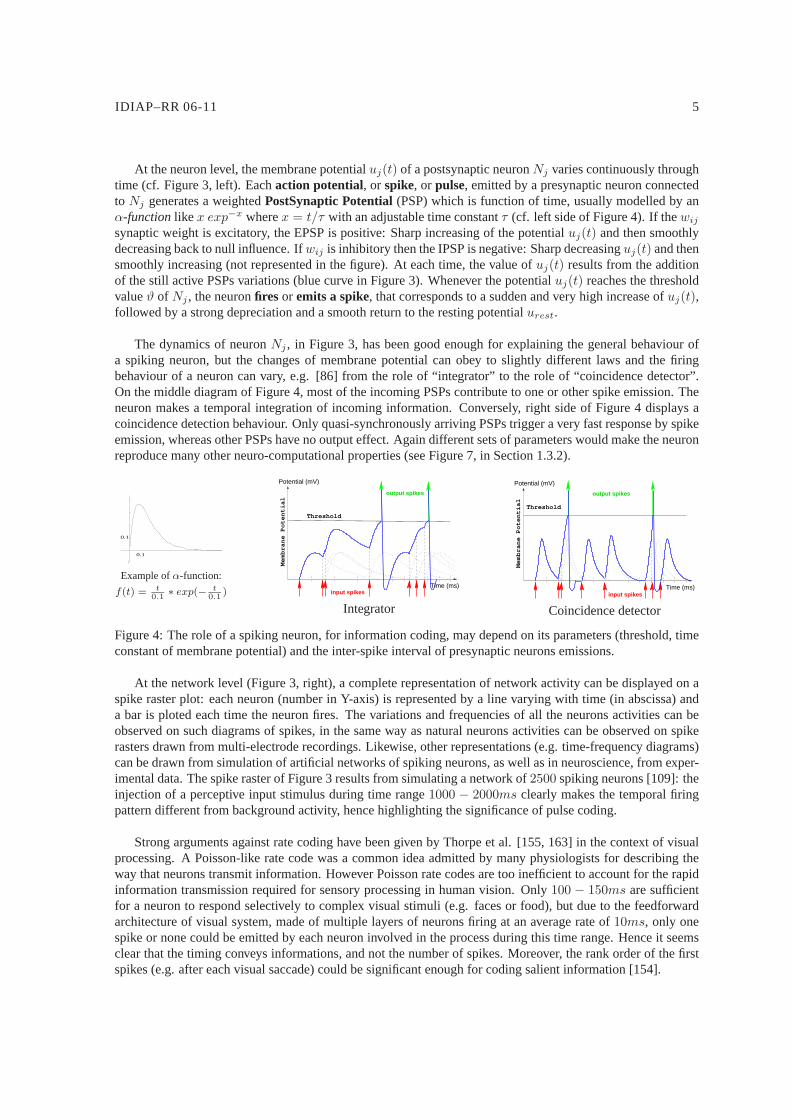

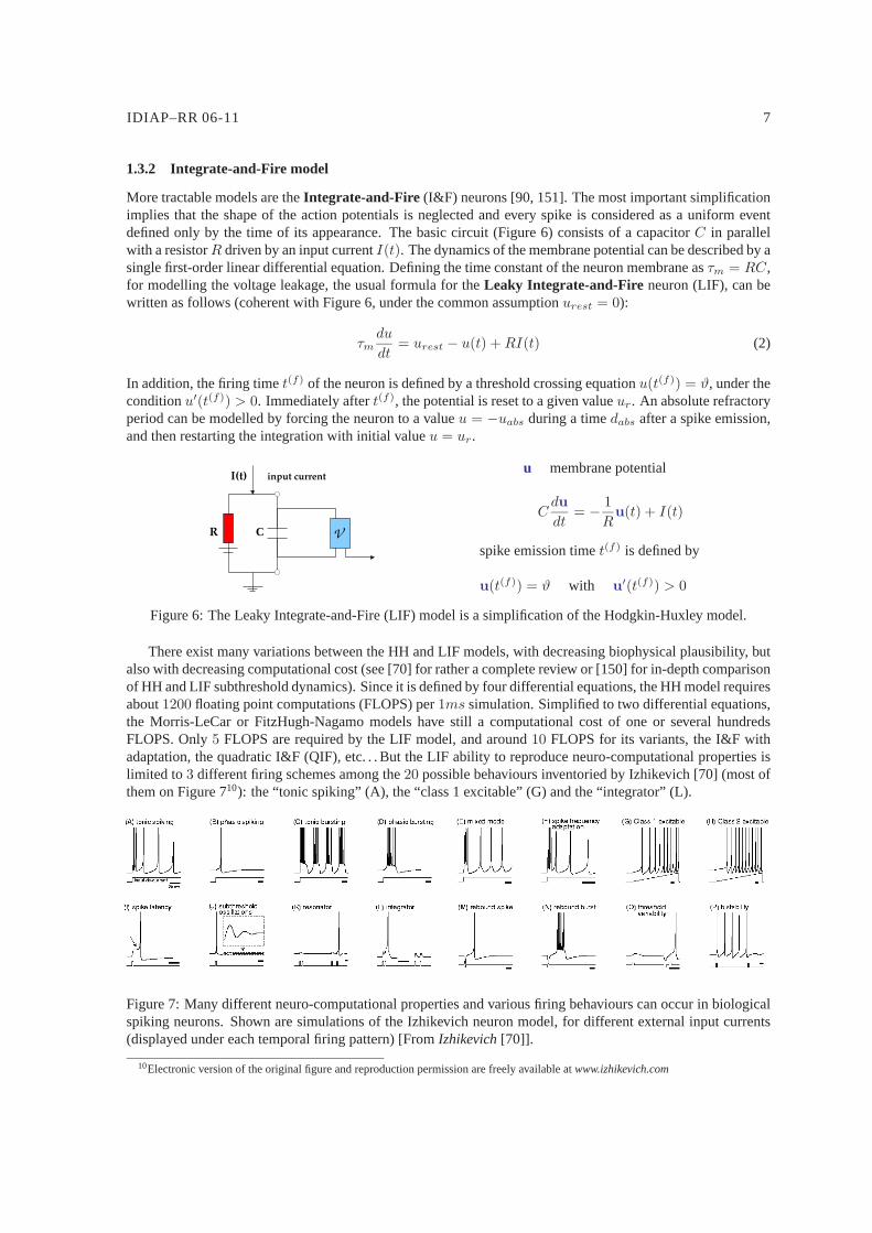


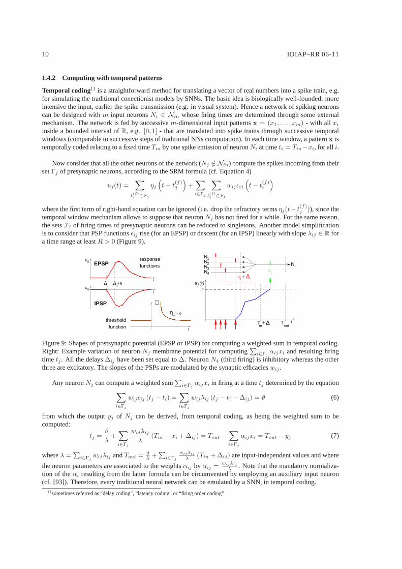


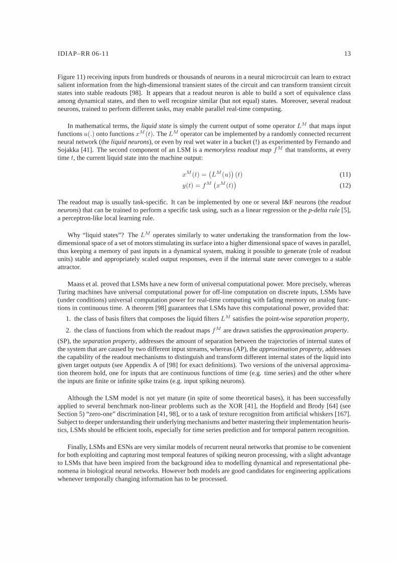

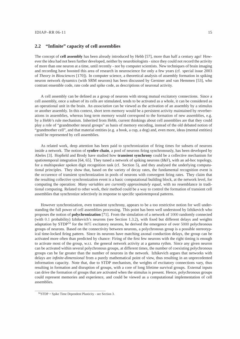


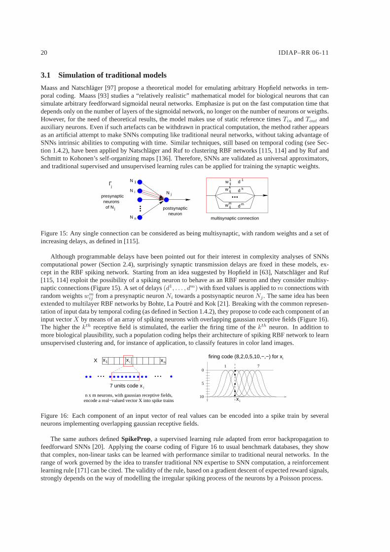


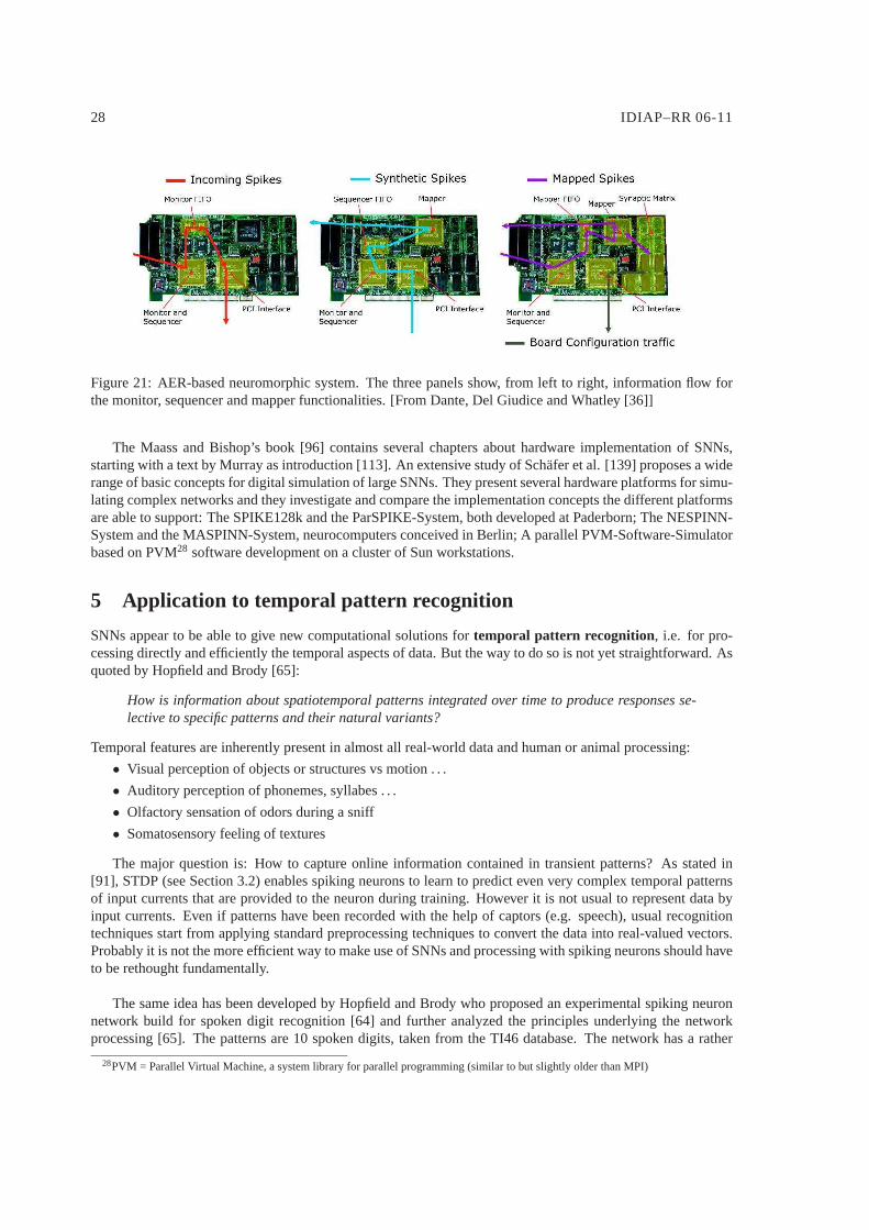
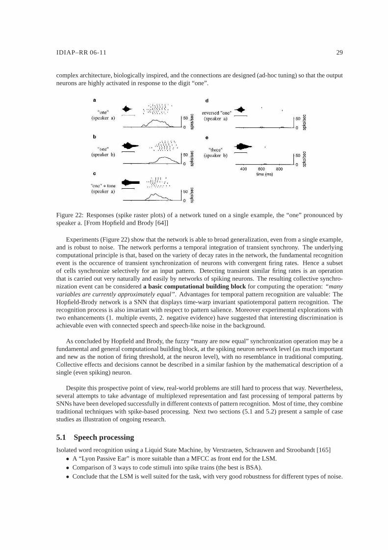


![Overconvergent global analytic geometry - arXiv · PDF filearXiv:1410.7971v2 [math.AG] 6 Feb 2015 Overconvergent global analytic geometry Frédéric Paugam February 9, 2015 “The](https://static.documents.pub/doc/80x56/5a7a04f37f8b9ab83f8d83b4/overconvergent-global-analytic-geometry-arxiv-14107971v2-mathag-6-feb-2015.jpg)


