118
R-INLA: An R-package for INLA Jingyi Guo <[email protected]> Department of Mathematical Sciences, NTNU April 14 2016 www.ntnu.no J. G., R-INLA: An R-package for INLA

R-INLA: An R-package for INLA
Jingyi Guo <[email protected]>
Department of Mathematical Sciences, NTNU
April 14 2016
www.ntnu.no J. G., R-INLA: An R-package for INLA
2
Outline
Structure of an R-INLA program
Simple example
Random effects
Model choice/checking
Useful features
www.ntnu.no J. G., R-INLA: An R-package for INLA
3
The structure of R-INLA
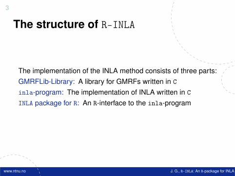
The implementation of the INLA method consists of three parts:GMRFLib-Library: A library for GMRFs written in C
inla-program: The implementation of INLA written in C
INLA package for R: An R-interface to the inla-program
www.ntnu.no J. G., R-INLA: An R-package for INLA

4
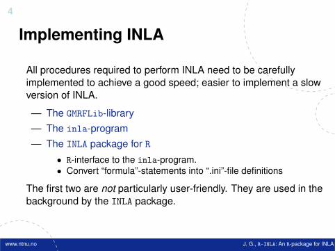
Implementing INLA
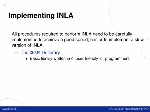
All procedures required to perform INLA need to be carefullyimplemented to achieve a good speed; easier to implement a slowversion of INLA.
— The GMRFLib-library— The inla-program— The INLA package for R
The first two are not particularly user-friendly. They are used in thebackground by the INLA package.
www.ntnu.no J. G., R-INLA: An R-package for INLA
4
Implementing INLA
All procedures required to perform INLA need to be carefullyimplemented to achieve a good speed; easier to implement a slowversion of INLA.
— The GMRFLib-library• Basic library written in C, user friendly for programmers
— The inla-program— The INLA package for R
The first two are not particularly user-friendly. They are used in thebackground by the INLA package.
www.ntnu.no J. G., R-INLA: An R-package for INLA
4
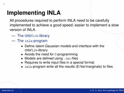
Implementing INLAAll procedures required to perform INLA need to be carefullyimplemented to achieve a good speed; easier to implement a slowversion of INLA.
— The GMRFLib-library— The inla-program
• Define latent Gaussian models and interface with theGMRFLib-library
• Avoids the need for C-programming• Models are defined using .ini-files• Requires to write input files in a special format• inla-program write all the results (E/Var/marginals) to files
— The INLA package for R
The first two are not particularly user-friendly. They are used in thebackground by the INLA package.
www.ntnu.no J. G., R-INLA: An R-package for INLA
4
Implementing INLA
All procedures required to perform INLA need to be carefullyimplemented to achieve a good speed; easier to implement a slowversion of INLA.
— The GMRFLib-library— The inla-program— The INLA package for R
• R-interface to the inla-program.• Convert “formula”-statements into “.ini”-file definitions
The first two are not particularly user-friendly. They are used in thebackground by the INLA package.
www.ntnu.no J. G., R-INLA: An R-package for INLA
5
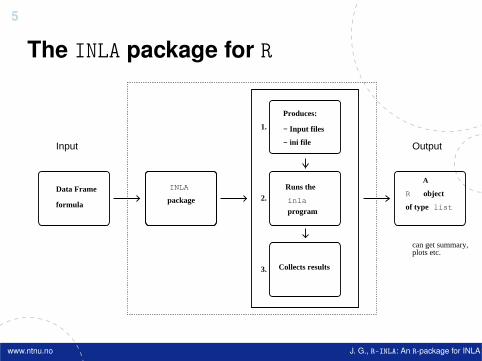
The INLA package for R
Data Frame
formula
− ini file
− Input files
Produces:
1.
2.
3.
inla
program
INLA
package
Collects results
Input
ARuns the
R
of type list
object
Output
plots etc.can get summary,
www.ntnu.no J. G., R-INLA: An R-package for INLA
6
Getting R-INLA— The web page www.r-inla.org contains source-code,
worked-through examples, reports and instructions forinstalling the package. INLA tutorial is in preparation.
— The R-package R-INLA works on Linux, Windows and Macand can be installed by
1 install.packages("INLA",2 repos="http://www.math.ntnu.no/inla/R/testing")
Later, it can be upgraded with1 update.packages(oldPkgs="INLA",2 repos="http://www.math.ntnu.no/inla/R/testing")
www.ntnu.no J. G., R-INLA: An R-package for INLA
6
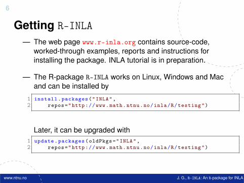
Getting R-INLA— The web page www.r-inla.org contains source-code,
worked-through examples, reports and instructions forinstalling the package. INLA tutorial is in preparation.
— The R-package R-INLA works on Linux, Windows and Macand can be installed by
1 install.packages("INLA",2 repos="http://www.math.ntnu.no/inla/R/testing")
Later, it can be upgraded with1 update.packages(oldPkgs="INLA",2 repos="http://www.math.ntnu.no/inla/R/testing")
www.ntnu.no J. G., R-INLA: An R-package for INLA
7
Documentation
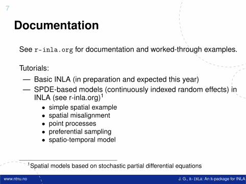
See r-inla.org for documentation and worked-through examples.
Tutorials:— Basic INLA (in preparation and expected this year)— SPDE-based models (continuously indexed random effects) in
INLA (see r-inla.org)1
• simple spatial example• spatial misalignment• point processes• preferential sampling• spatio-temporal model
1Spatial models based on stochastic partial differential equations
www.ntnu.no J. G., R-INLA: An R-package for INLA
8
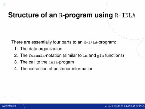
Structure of an R-program using R-INLA
There are essentially four parts to an R-INLA-program:1. The data organization2. The formula-notation (similar to lm and glm functions)3. The call to the inla-progam4. The extraction of posterior information
www.ntnu.no J. G., R-INLA: An R-package for INLA
9
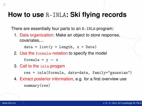
How to use R-INLA: Ski flying records
There are essentially four parts to an R-INLA-program:1. Data organization: Make an object to store response,
covariates,...data = list(y = Length, x = Date)
2. Use the formula-notation to specify the modelformula = y ∼ x
3. Call to the inla-progamres = inla(formula, data=data, family="gaussian")
4. Extract posterior information, e.g. for a first overview usesummary(res)
www.ntnu.no J. G., R-INLA: An R-package for INLA
10
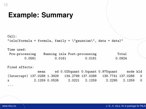
Example: Summary
Call:"inla(formula = formula, family = \"gaussian\", data = data)"
Time used:Pre-processing Running inla Post-processing Total
0.0581 0.0161 0.0181 0.0924
Fixed effects:mean sd 0.025quant 0.5quant 0.975quant mode kld
(Intercept) 137.0288 1.3929 134.2798 137.0288 139.7741 137.0288 0x 2.1259 0.0526 2.0221 2.1259 2.2295 2.1259 0...
www.ntnu.no J. G., R-INLA: An R-package for INLA
11
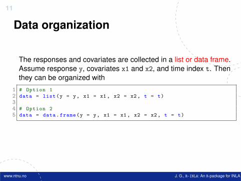
Data organization
The responses and covariates are collected in a list or data frame.Assume response y, covariates x1 and x2, and time index t. Thenthey can be organized with
1 # Option 12 data = list(y = y, x1 = x1, x2 = x2 , t = t)34 # Option 25 data = data.frame(y = y, x1 = x1 , x2 = x2, t = t)
www.ntnu.no J. G., R-INLA: An R-package for INLA

12
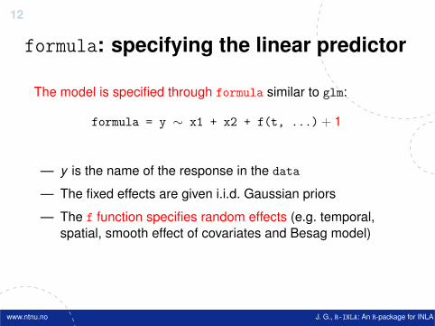
formula: specifying the linear predictor
The model is specified through formula similar to glm:
formula = y ∼ x1 + x2 + f(t, ...)
+ 1− 1
— y is the name of the response in the data
— The fixed effects are given i.i.d. Gaussian priors
— The f function specifies random effects (e.g. temporal,spatial, smooth effect of covariates and Besag model)
— Use -1 if you don’t want an automatic intercept
www.ntnu.no J. G., R-INLA: An R-package for INLA
12
formula: specifying the linear predictor
The model is specified through formula similar to glm:
formula = y ∼ x1 + x2 + f(t, ...)+ 1
− 1
— y is the name of the response in the data
— The fixed effects are given i.i.d. Gaussian priors
— The f function specifies random effects (e.g. temporal,spatial, smooth effect of covariates and Besag model)
— Use -1 if you don’t want an automatic intercept
www.ntnu.no J. G., R-INLA: An R-package for INLA

12
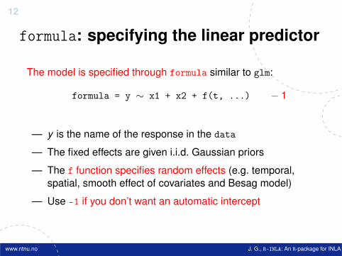
formula: specifying the linear predictor
The model is specified through formula similar to glm:
formula = y ∼ x1 + x2 + f(t, ...)
+ 1− 1
— y is the name of the response in the data
— The fixed effects are given i.i.d. Gaussian priors
— The f function specifies random effects (e.g. temporal,spatial, smooth effect of covariates and Besag model)
— Use -1 if you don’t want an automatic intercept
www.ntnu.no J. G., R-INLA: An R-package for INLA
12
formula: specifying the linear predictor
The model is specified through formula similar to glm:
formula = y ∼ x1 + x2 + f(t, ...)
+ 1
− 1
— y is the name of the response in the data
— The fixed effects are given i.i.d. Gaussian priors
— The f function specifies random effects (e.g. temporal,spatial, smooth effect of covariates and Besag model)
— Use -1 if you don’t want an automatic intercept
www.ntnu.no J. G., R-INLA: An R-package for INLA
13
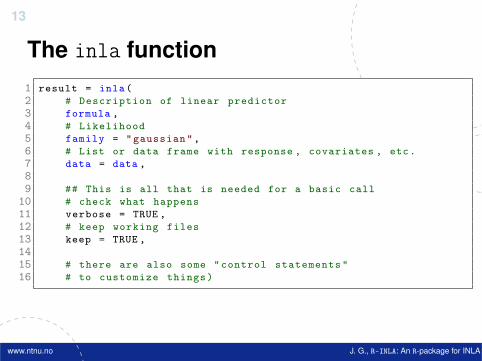
The inla function1 result = inla(2 # Description of linear predictor3 formula ,4 # Likelihood5 family = "gaussian",6 # List or data frame with response , covariates , etc.7 data = data ,89 ## This is all that is needed for a basic call
10 # check what happens11 verbose = TRUE ,12 # keep working files13 keep = TRUE ,1415 # there are also some "control statements"16 # to customize things)
www.ntnu.no J. G., R-INLA: An R-package for INLA
14
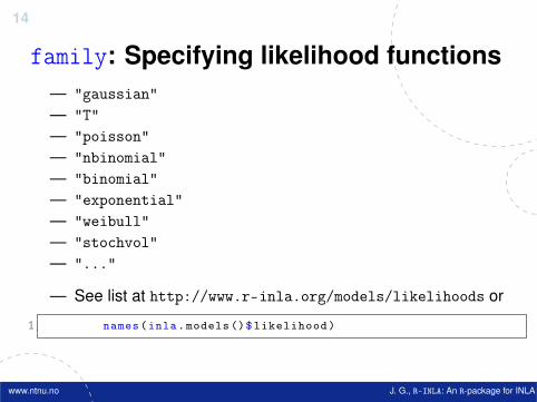
family: Specifying likelihood functions— "gaussian"— "T"— "poisson"— "nbinomial"— "binomial"— "exponential"— "weibull"— "stochvol"— "..."
— See list at http://www.r-inla.org/models/likelihoods or
1 names(inla.models ()$likelihood)
www.ntnu.no J. G., R-INLA: An R-package for INLA
15
What can we get: Posterior inference
Main functions:— summary(result)
— plot(result)
www.ntnu.no J. G., R-INLA: An R-package for INLA
16
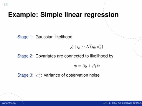
Example: Simple linear regression
Stage 1: Gaussian likelihood
yi | ηi ∼ N (ηi , σ2o)
Stage 2: Covariates are connected to likelihood by
ηi = β0 + β1xi
Stage 3: σ2o : variance of observation noise
www.ntnu.no J. G., R-INLA: An R-package for INLA
17
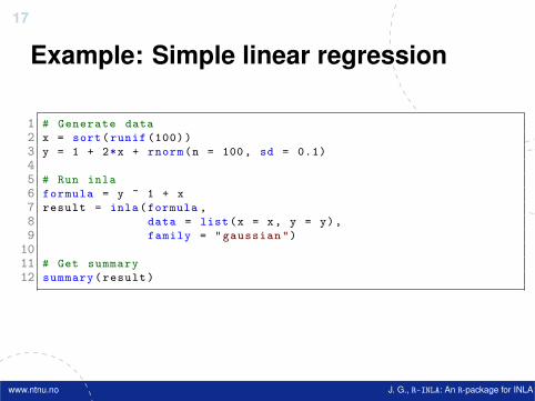
Example: Simple linear regression
1 # Generate data2 x = sort(runif (100))3 y = 1 + 2*x + rnorm(n = 100, sd = 0.1)45 # Run inla6 formula = y ~ 1 + x7 result = inla(formula ,8 data = list(x = x, y = y),9 family = "gaussian")
1011 # Get summary12 summary(result)
www.ntnu.no J. G., R-INLA: An R-package for INLA
18
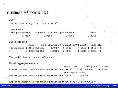
summary(result)Call:"inla(formula = y ~ x, data = data)"
Time used:Pre-processing Running inla Post-processing Total
0.3198 0.0396 0.0352 0.3946
Fixed effects:mean sd 0.025quant 0.5quant 0.975quant mode kld
(Intercept) 1.0140 0.0195 0.9757 1.0140 1.0523 1.0140 0x 2.0025 0.0316 1.9405 2.0025 2.0645 2.0025 0
The model has no random effects
Model hyperparameters:mean sd 0.025quant 0.5quant
Precision for the Gaussian observations 114.87 16.28 85.66 113.980.975quant mode
Precision for the Gaussian observations 149.37 112.42
Expected number of effective parameters(std dev): 2.189(0.0213)Number of equivalent replicates : 45.69
Marginal Likelihood: 78.36
www.ntnu.no J. G., R-INLA: An R-package for INLA
19
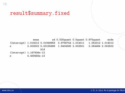
result$summary.fixed
mean sd 0.025quant 0.5quant 0.975quant mode(Intercept) 1.014012 0.01949959 0.9756744 1.014011 1.052312 1.014012x 2.002502 0.03155688 1.9404595 2.002501 2.064484 2.002502
kld(Intercept) 1.167936e-12x 4.459456e-13
www.ntnu.no J. G., R-INLA: An R-package for INLA
20
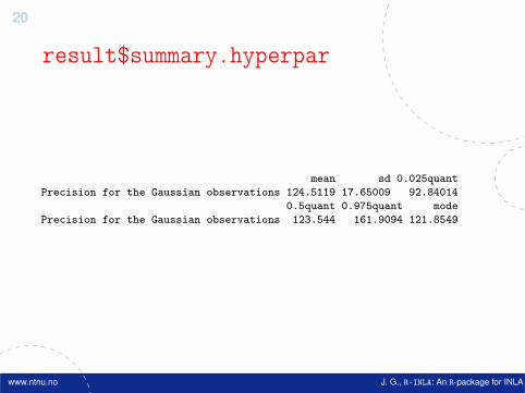
result$summary.hyperpar
mean sd 0.025quantPrecision for the Gaussian observations 124.5119 17.65009 92.84014
0.5quant 0.975quant modePrecision for the Gaussian observations 123.544 161.9094 121.8549
www.ntnu.no J. G., R-INLA: An R-package for INLA
21
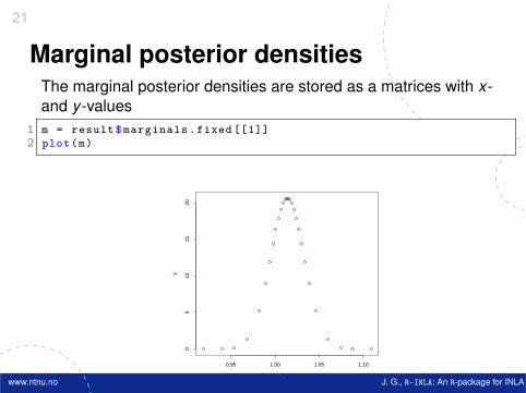
Marginal posterior densitiesThe marginal posterior densities are stored as a matrices with x-and y -values
1 m = result$marginals.fixed [[1]]2 plot(m)
0.95 1.00 1.05 1.10
05
1015
20
x
y
www.ntnu.no J. G., R-INLA: An R-package for INLA
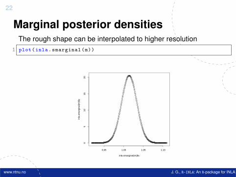
22
Marginal posterior densitiesThe rough shape can be interpolated to higher resolution
1 plot(inla.smarginal(m))
0.95 1.00 1.05 1.10
05
1015
20
inla.smarginal(m)$x
inla
.sm
argi
nal(m
)$y
www.ntnu.no J. G., R-INLA: An R-package for INLA
23
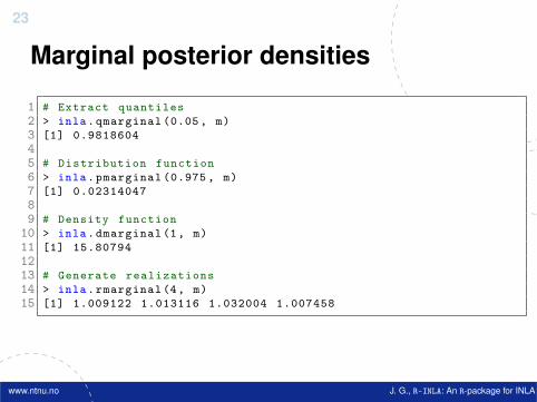
Marginal posterior densities
1 # Extract quantiles2 > inla.qmarginal (0.05, m)3 [1] 0.981860445 # Distribution function6 > inla.pmarginal (0.975 , m)7 [1] 0.0231404789 # Density function
10 > inla.dmarginal(1, m)11 [1] 15.807941213 # Generate realizations14 > inla.rmarginal(4, m)15 [1] 1.009122 1.013116 1.032004 1.007458
www.ntnu.no J. G., R-INLA: An R-package for INLA
24
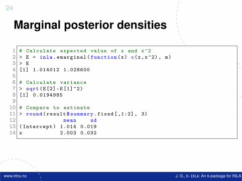
Marginal posterior densities
1 # Calculate expected value of x and x^22 > E = inla.emarginal(function(x) c(x,x^2), m)3 > E4 [1] 1.014012 1.02860056 # Calculate variance7 > sqrt(E[2]-E[1]^2)8 [1] 0.01949859
10 # Compare to estimate11 > round(result$summary.fixed [,1:2], 3)12 mean sd13 (Intercept) 1.014 0.01914 x 2.003 0.032
www.ntnu.no J. G., R-INLA: An R-package for INLA
25
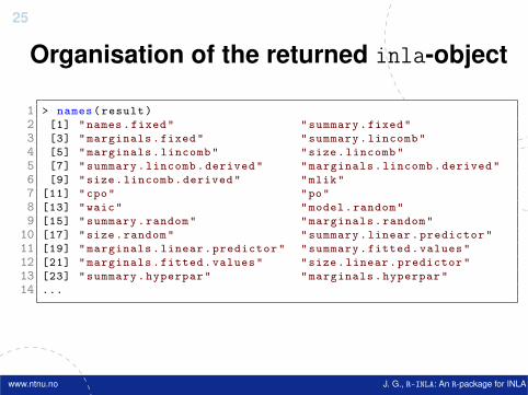
Organisation of the returned inla-object
1 > names(result)2 [1] "names.fixed" "summary.fixed"3 [3] "marginals.fixed" "summary.lincomb"4 [5] "marginals.lincomb" "size.lincomb"5 [7] "summary.lincomb.derived" "marginals.lincomb.derived"6 [9] "size.lincomb.derived" "mlik"7 [11] "cpo" "po"8 [13] "waic" "model.random"9 [15] "summary.random" "marginals.random"
10 [17] "size.random" "summary.linear.predictor"11 [19] "marginals.linear.predictor" "summary.fitted.values"12 [21] "marginals.fitted.values" "size.linear.predictor"13 [23] "summary.hyperpar" "marginals.hyperpar"14 ...
www.ntnu.no J. G., R-INLA: An R-package for INLA
26
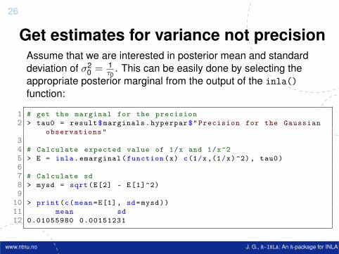
Get estimates for variance not precisionAssume that we are interested in posterior mean and standarddeviation of σ2
0 = 1τ0
. This can be easily done by selecting theappropriate posterior marginal from the output of the inla()function:
1 # get the marginal for the precision2 > tau0 = result$marginals.hyperpar$"Precision for the Gaussian
observations"34 # Calculate expected value of 1/x and 1/x^25 > E = inla.emarginal(function(x) c(1/x,(1/x)^2), tau0)67 # Calculate sd8 > mysd = sqrt(E[2] - E[1]^2)9
10 > print(c(mean=E[1], sd=mysd))11 mean sd12 0.01055980 0.00151231
www.ntnu.no J. G., R-INLA: An R-package for INLA
27
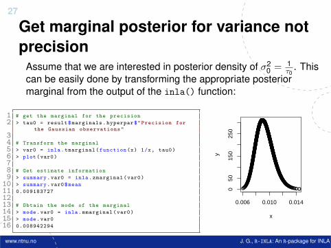
Get marginal posterior for variance notprecision
Assume that we are interested in posterior density of σ20 = 1
τ0. This
can be easily done by transforming the appropriate posteriormarginal from the output of the inla() function:
1 # get the marginal for the precision2 > tau0 = result$marginals.hyperpar$"Precision for
the Gaussian observations"34 # Transform the marginal5 > var0 = inla.tmarginal(function(x) 1/x, tau0)6 > plot(var0)78 # Get estimate information9 > summary.var0 = inla.zmarginal(var0)
10 > summary.var0$mean11 0.0091837271213 # Obtain the mode of the marginal14 > mode.var0 = inla.mmarginal(var0)15 > mode.var016 0.008942294
●●●●●●●●●●●●●●●●●●●●●●●●●●●●●●●●●●●●●●●●●●●●●●●●●●●●●●●●●●●●●●●●●●●●●●●●●●●●●●●●●●●●●●●●●●●●●●●●●●●●●●●●●●●●●●●●●●●●●●●●●●●●●●●●●●●●●●●●●●●●●●●●●●●●●●●●●●●●●●●●●●●●●●●●●●●●●●●●●●●●●●●●●●●●●●●●●●●●●●●●●●●●●●●●●●●●●●●●●●●●●●●●●●●●●●●●●●●●●●●●●●●●●●●●●●●●●●●●●●●●●●●●●●●●●●●●●●●●●●●●●●●●●●●●●●●●●●●●●●●●●●●●●●●●●●●●●●●●●●●●●●●●●●●●●●●●●●●●●●●●●●●●●●●●●●●●●●●●●●●●●●●●●●●●●●●●●●●●●●●●●●●●●●●●●●●●●●●●●●●●●●●●●●●●●●●●●●●●●●●●●●●●●●●●●●●●●●●●●●●●●●●●●●●●●●●●●●●●●●●●●●●●●●●●●●●●●●●●●●●●●●●●●●●●●●●●●●●●●●●●●●●●●●●●●●●●●●●●●●●●●●●●●●●●●●●●●●●●●●●●●●●●●●●●●●●●●●●●●●●●●●●●●●●●●●●●●●●●●●●●●●●●●●●●●●●●●●●●●●●●●●●●●●●●●●●●●●●●●●●●●●●●●●●●●●●●●●●●●●●●●●●●●●●●●●●●●●●●●●●●●●●●●●●●●●●●●●●●●●●●●●●●●●●●●●●●●●●●●●●●●●●●●●●●●●●●●●●●●●●●●●●●●●●●●●●●●●●●●●●●●●●●●●●●●●●●●●●●●●●●●●●●●●●●●●●●●●●●●●●●●●●●●●●●●●●●●●●●●●●●●●●●●●●●●●●●●●●●●●●●●●●●●●●●●●●●●●●●●●●●●●●●●●●●●●●●●●●●●●●●●●●●●●●●●●●●●●●●●●●●●●●●●●●●●●●●●●●●●●●●●●●●●●●●●●●●●●●●●●●●●●●●●●●●●●●●●●●●●●●●●●●●●●●●●●●●●●●●●●●●●●●●●●●●●●●●●●●●●●●●●●●●●●●●●●●●●●●●●●●●●●●●●●●●●●●●●●●●●●●●●●●●
0.006 0.010 0.014
050
150
250
xy
www.ntnu.no J. G., R-INLA: An R-package for INLA
28
Example: Count data of crime
contains data on arrests during the year 1986 and otherinformation on 2,725 men born in either 1960 or 1961 in California.Each man in the sample was arrested at least once prior to 1986.— y = the number of times a man is arrested during 1986.— x1 = the proportion of prior arrests that led to a conviction.— x2 = the average sentence served from prior convictions (in
months).— x3 = months spent in prison since age 18 prior to 1986.— x4 = months spent in prison in 1986.
www.ntnu.no J. G., R-INLA: An R-package for INLA
29
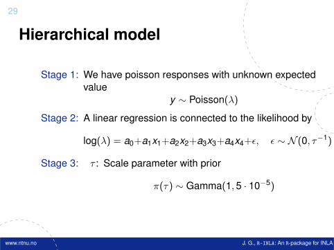
Hierarchical model
Stage 1: We have poisson responses with unknown expectedvalue
y ∼ Poisson(λ)
Stage 2: A linear regression is connected to the likelihood by
log(λ) = a0+a1x1+a2x2+a3x3+a4x4+ε, ε ∼ N (0, τ−1)
Stage 3: τ : Scale parameter with prior
π(τ) ∼ Gamma(1,5 · 10−5)
www.ntnu.no J. G., R-INLA: An R-package for INLA
30
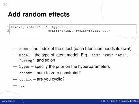
Add random effects
1 f(name , model="...", hyper =...,2 constr=FALSE , cyclic=FALSE , ...)
— name – the index of the effect (each f-function needs its own!)— model – the type of latent model. E.g. "iid", "rw2", "ar1",
"besag", and so on— hyper – specify the prior on the hyperparameters— constr – sum-to-zero constraint?— cyclic – are you cyclic?— . . .
www.ntnu.no J. G., R-INLA: An R-package for INLA
31
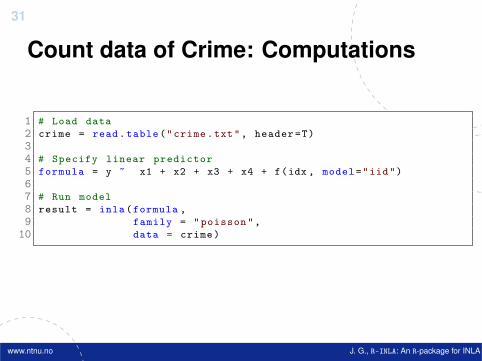
Count data of Crime: Computations
1 # Load data2 crime = read.table("crime.txt", header=T)34 # Specify linear predictor5 formula = y ~ x1 + x2 + x3 + x4 + f(idx , model="iid")67 # Run model8 result = inla(formula ,9 family = "poisson",
10 data = crime)
www.ntnu.no J. G., R-INLA: An R-package for INLA
32
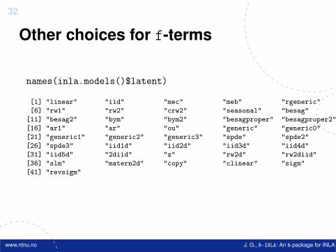
Other choices for f-terms
names(inla.models()$latent)
[1] "linear" "iid" "mec" "meb" "rgeneric"[6] "rw1" "rw2" "crw2" "seasonal" "besag"
[11] "besag2" "bym" "bym2" "besagproper" "besagproper2"[16] "ar1" "ar" "ou" "generic" "generic0"[21] "generic1" "generic2" "generic3" "spde" "spde2"[26] "spde3" "iid1d" "iid2d" "iid3d" "iid4d"[31] "iid5d" "2diid" "z" "rw2d" "rw2diid"[36] "slm" "matern2d" "copy" "clinear" "sigm"[41] "revsigm"
www.ntnu.no J. G., R-INLA: An R-package for INLA
33
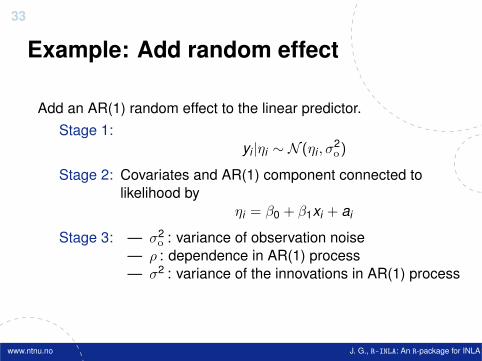
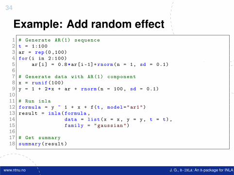
Example: Add random effect
Add an AR(1) random effect to the linear predictor.Stage 1:
yi |ηi ∼ N (ηi , σ2o)
Stage 2: Covariates and AR(1) component connected tolikelihood by
ηi = β0 + β1xi + ai
Stage 3: — σ2o : variance of observation noise
— ρ : dependence in AR(1) process— σ2 : variance of the innovations in AR(1) process
www.ntnu.no J. G., R-INLA: An R-package for INLA
34
Example: Add random effect1 # Generate AR(1) sequence2 t = 1:1003 ar = rep (0 ,100)4 for(i in 2:100)5 ar[i] = 0.8*ar[i-1]+ rnorm(n = 1, sd = 0.1)67 # Generate data with AR(1) component8 x = runif (100)9 y = 1 + 2*x + ar + rnorm(n = 100, sd = 0.1)
1011 # Run inla12 formula = y ~ 1 + x + f(t, model="ar1")13 result = inla(formula ,14 data = list(x = x, y = y, t = t),15 family = "gaussian")1617 # Get summary18 summary(result)
www.ntnu.no J. G., R-INLA: An R-package for INLA
35
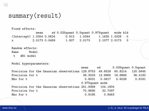
summary(result)
Fixed effects:mean sd 0.025quant 0.5quant 0.975quant mode kld
(Intercept) 1.0354 0.0624 0.913 1.0344 1.1635 1.0328 0x 2.0173 0.0459 1.927 2.0173 2.1077 2.0173 0
Random effects:Name Modelt AR1 model
Model hyperparameters:mean sd 0.025quant 0.5quant
Precision for the Gaussian observations 129.8753 49.6529 60.8214 120.5645Precision for t 38.3033 13.9965 16.8866 36.4192Rho for t 0.8031 0.0817 0.6028 0.8181
0.975quant modePrecision for the Gaussian observations 251.9389 104.1904Precision for t 70.9695 32.7097Rho for t 0.9185 0.8463
www.ntnu.no J. G., R-INLA: An R-package for INLA
36
The interpretation of NA
R-INLA uses NA differently than other packages— NA in the response means no likelihood contribution,
i.e. response is unobserved— NA in a fixed effect means no contribution to the linear
predictor, i.e. the covariate is set equal to zero— NA in a random effect f(...) means no contribution to the
linear predictor
www.ntnu.no J. G., R-INLA: An R-package for INLA
37
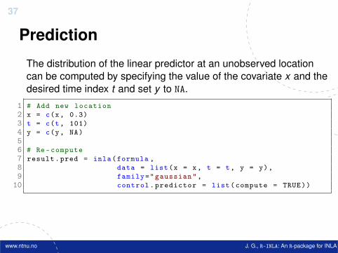
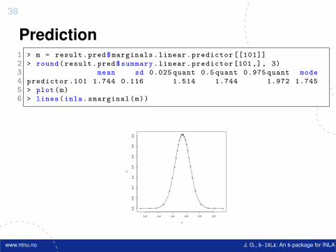
Prediction
The distribution of the linear predictor at an unobserved locationcan be computed by specifying the value of the covariate x and thedesired time index t and set y to NA.
1 # Add new location2 x = c(x, 0.3)3 t = c(t, 101)4 y = c(y, NA)56 # Re-compute7 result.pred = inla(formula ,8 data = list(x = x, t = t, y = y),9 family="gaussian",
10 control.predictor = list(compute = TRUE))
www.ntnu.no J. G., R-INLA: An R-package for INLA
38
Prediction1 > m = result.pred$marginals.linear.predictor [[101]]2 > round(result.pred$summary.linear.predictor [101,], 3)3 mean sd 0.025 quant 0.5 quant 0.975 quant mode4 predictor .101 1.744 0.116 1.514 1.744 1.972 1.7455 > plot(m)6 > lines(inla.smarginal(m))
1.2 1.4 1.6 1.8 2.0 2.2
0.0
0.5
1.0
1.5
2.0
2.5
3.0
3.5
x
y
www.ntnu.no J. G., R-INLA: An R-package for INLA
39
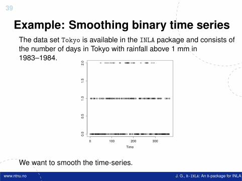
Example: Smoothing binary time seriesThe data set Tokyo is available in the INLA package and consists ofthe number of days in Tokyo with rainfall above 1 mm in1983–1984.
0 100 200 300
0.0
0.5
1.0
1.5
2.0
Time
We want to smooth the time-series.
www.ntnu.no J. G., R-INLA: An R-package for INLA
40
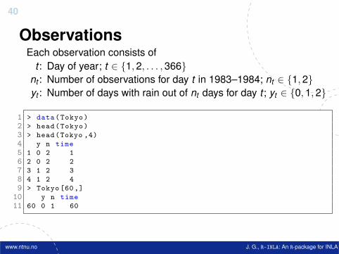
ObservationsEach observation consists of
t : Day of year; t ∈ {1,2, . . . ,366}nt : Number of observations for day t in 1983–1984; nt ∈ {1,2}yt : Number of days with rain out of nt days for day t ; yt ∈ {0,1,2}
1 > data(Tokyo)2 > head(Tokyo)3 > head(Tokyo ,4)4 y n time5 1 0 2 16 2 0 2 27 3 1 2 38 4 1 2 49 > Tokyo [60,]
10 y n time11 60 0 1 60
www.ntnu.no J. G., R-INLA: An R-package for INLA
41
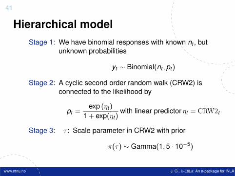
Hierarchical modelStage 1: We have binomial responses with known nt , but
unknown probabilities
yt ∼ Binomial(nt ,pt)
Stage 2: A cyclic second order random walk (CRW2) isconnected to the likelihood by
pt =exp (ηt)
1 + exp(ηt)with linear predictor ηt = CRW2t
Stage 3: τ : Scale parameter in CRW2 with prior
π(τ) ∼ Gamma(1,5 · 10−5)
www.ntnu.no J. G., R-INLA: An R-package for INLA
42
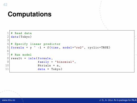
Computations
1 # Read data2 data(Tokyo)34 # Specify linear predictor5 formula = y ~ -1 + f(time , model="rw2", cyclic=TRUE)67 # Run model8 result = inla(formula ,9 family = "binomial",
10 Ntrials = n,11 data = Tokyo)
www.ntnu.no J. G., R-INLA: An R-package for INLA
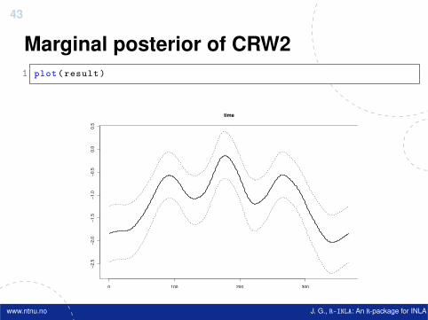
43
Marginal posterior of CRW21 plot(result)
0 100 200 300
−2.5
−2.0
−1.5
−1.0
−0.5
0.0
0.5
time
www.ntnu.no J. G., R-INLA: An R-package for INLA
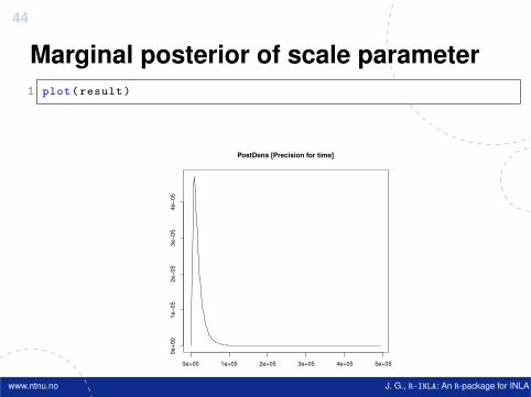
44
Marginal posterior of scale parameter1 plot(result)
0e+00 1e+05 2e+05 3e+05 4e+05 5e+05
0e+
00
1e−
05
2e−
05
3e−
05
4e−
05
PostDens [Precision for time]
www.ntnu.no J. G., R-INLA: An R-package for INLA
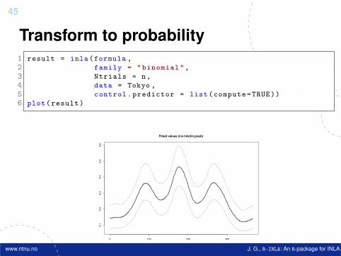
45
Transform to probability1 result = inla(formula ,2 family = "binomial",3 Ntrials = n,4 data = Tokyo ,5 control.predictor = list(compute=TRUE))6 plot(result)
0 100 200 300
0.1
0.2
0.3
0.4
0.5
0.6
Fitted values (inv.link(lin.pred))
www.ntnu.no J. G., R-INLA: An R-package for INLA
46
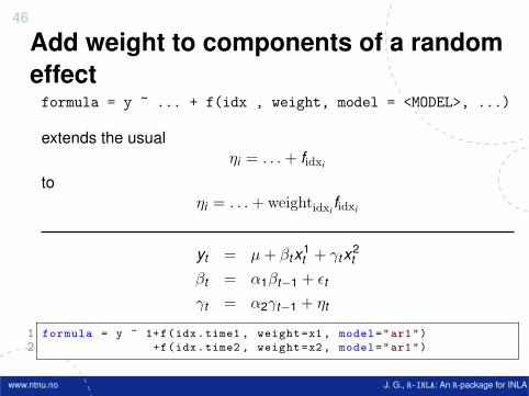
Add weight to components of a randomeffectformula = y ~ ... + f(idx , weight, model = <MODEL>, ...)
extends the usualηi = . . .+ fidxi
toηi = . . .+ weightidxi
fidxi
yt = µ+ βtx1t + γtx2
t
βt = α1βt−1 + εt
γt = α2γt−1 + ηt
1 formula = y ~ 1+f(idx.time1 , weight=x1, model="ar1")2 +f(idx.time2 , weight=x2 , model="ar1")
www.ntnu.no J. G., R-INLA: An R-package for INLA
47
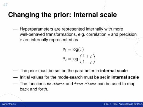
Changing the prior: Internal scale
— Hyperparameters are represented internally with morewell-behaved transformations, e.g. correlation ρ and precisionτ are internally represented as
θ1 = log(τ)
θ2 = log(
1 + ρ
1− ρ
)— The prior must be set on the parameter in internal scale— Initial values for the mode-search must be set in internal scale— The functions to.theta and from.theta can be used to map
back and forth.
www.ntnu.no J. G., R-INLA: An R-package for INLA
48
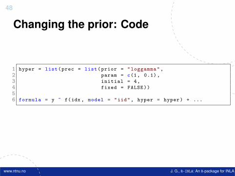
Changing the prior: Code
1 hyper = list(prec = list(prior = "loggamma",2 param = c(1, 0.1),3 initial = 4,4 fixed = FALSE))56 formula = y ~ f(idx , model = "iid", hyper = hyper) + ...
www.ntnu.no J. G., R-INLA: An R-package for INLA
49
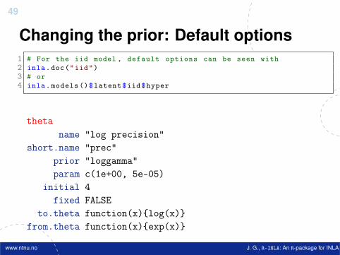
Changing the prior: Default options1 # For the iid model , default options can be seen with2 inla.doc("iid")3 # or4 inla.models ()$latent$iid$hyper
thetaname "log precision"
short.name "prec"prior "loggamma"param c(1e+00, 5e-05)
initial 4fixed FALSE
to.theta function(x){log(x)}from.theta function(x){exp(x)}
www.ntnu.no J. G., R-INLA: An R-package for INLA
50
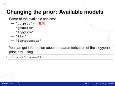
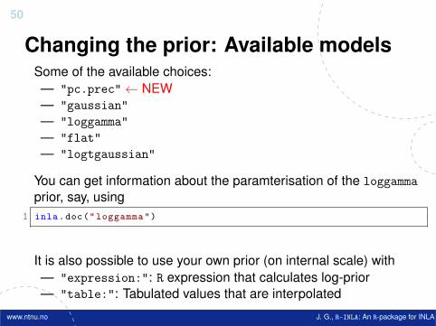
Changing the prior: Available modelsSome of the available choices:— "pc.prec"← NEW— "gaussian"— "loggamma"— "flat"— "logtgaussian"
You can get information about the paramterisation of the loggammaprior, say, using
1 inla.doc("loggamma")
It is also possible to use your own prior (on internal scale) with— "expression:": R expression that calculates log-prior— "table:": Tabulated values that are interpolated
www.ntnu.no J. G., R-INLA: An R-package for INLA
50
Changing the prior: Available modelsSome of the available choices:— "pc.prec"← NEW— "gaussian"— "loggamma"— "flat"— "logtgaussian"
You can get information about the paramterisation of the loggammaprior, say, using
1 inla.doc("loggamma")
It is also possible to use your own prior (on internal scale) with— "expression:": R expression that calculates log-prior— "table:": Tabulated values that are interpolated
www.ntnu.no J. G., R-INLA: An R-package for INLA
51
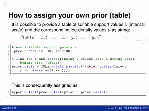
How to assign your own prior (table)It is possible to provide a table of suitable support values x (internalscale) and the corresponding log-density values y as string:
“table: x_1 ... x_n y_1 ... y_n”
1 # use suitable support points x2 lprec = seq(-10, 10, len =100)34 # link the x and corresponding y values into a string which
begins with "table :""5 prior.table = INLA ::: inla.paste(c("table:",cbind(lprec ,6 prior.function(lprec))))
This is consequently assigned as1 hyper = list(prec = list(prior = prior.table))
www.ntnu.no J. G., R-INLA: An R-package for INLA
52
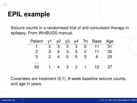
EPIL example
Seizure counts in a randomised trial of anti-convulsant therapy inepilepsy. From WinBUGS manual.
Patient y1 y2 y3 y4 Trt Base Age1 5 3 3 3 0 11 312 3 5 3 3 0 11 303 2 4 0 5 0 6 25
....59 1 4 3 2 1 12 37
Covariates are treatment (0,1), 8-week baseline seizure counts,and age in years.
www.ntnu.no J. G., R-INLA: An R-package for INLA
53
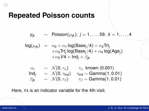
Repeated Poisson counts
yjk ∼ Poisson(µjk ); j = 1, . . . ,59; k = 1, . . . ,4
log(µjk ) = α0 + α1 log(Basej/4) + α2Trtj+α3Trtj log(Basej/4) + α4 log(Agej)
+α5V4 + Indj + βjk
αi ∼ N (0, τα) τα known (0.001)Indj ∼ N (0, τInd) τInd ∼ Gamma(1,0.01)βjk ∼ N (0, τβ) τβ ∼ Gamma(1,0.01)
Here, V4 is an indicator variable for the 4th visit.
www.ntnu.no J. G., R-INLA: An R-package for INLA
54
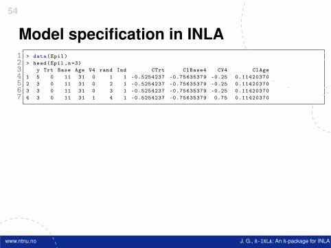
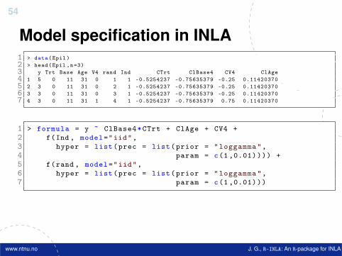
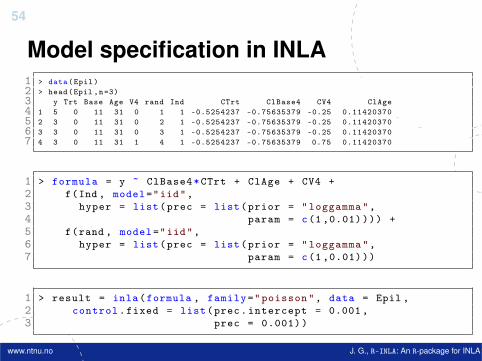
Model specification in INLA1 > data(Epil)2 > head(Epil ,n=3)3 y Trt Base Age V4 rand Ind CTrt ClBase4 CV4 ClAge4 1 5 0 11 31 0 1 1 -0.5254237 -0.75635379 -0.25 0.114203705 2 3 0 11 31 0 2 1 -0.5254237 -0.75635379 -0.25 0.114203706 3 3 0 11 31 0 3 1 -0.5254237 -0.75635379 -0.25 0.114203707 4 3 0 11 31 1 4 1 -0.5254237 -0.75635379 0.75 0.11420370
1 > formula = y ~ ClBase4*CTrt + ClAge + CV4 +2 f(Ind , model="iid",3 hyper = list(prec = list(prior = "loggamma",4 param = c(1 ,0.01)))) +5 f(rand , model="iid",6 hyper = list(prec = list(prior = "loggamma",7 param = c(1 ,0.01)))
1 > result = inla(formula , family="poisson", data = Epil ,2 control.fixed = list(prec.intercept = 0.001 ,3 prec = 0.001))
www.ntnu.no J. G., R-INLA: An R-package for INLA
54
Model specification in INLA1 > data(Epil)2 > head(Epil ,n=3)3 y Trt Base Age V4 rand Ind CTrt ClBase4 CV4 ClAge4 1 5 0 11 31 0 1 1 -0.5254237 -0.75635379 -0.25 0.114203705 2 3 0 11 31 0 2 1 -0.5254237 -0.75635379 -0.25 0.114203706 3 3 0 11 31 0 3 1 -0.5254237 -0.75635379 -0.25 0.114203707 4 3 0 11 31 1 4 1 -0.5254237 -0.75635379 0.75 0.11420370
1 > formula = y ~ ClBase4*CTrt + ClAge + CV4 +2 f(Ind , model="iid",3 hyper = list(prec = list(prior = "loggamma",4 param = c(1 ,0.01)))) +5 f(rand , model="iid",6 hyper = list(prec = list(prior = "loggamma",7 param = c(1 ,0.01)))
1 > result = inla(formula , family="poisson", data = Epil ,2 control.fixed = list(prec.intercept = 0.001 ,3 prec = 0.001))
www.ntnu.no J. G., R-INLA: An R-package for INLA
55
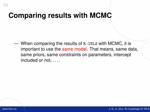
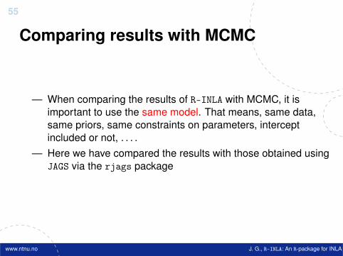
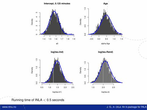
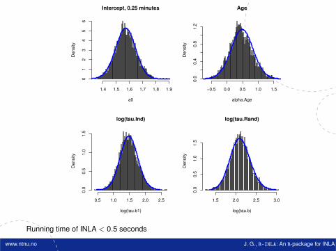
Comparing results with MCMC
— When comparing the results of R-INLA with MCMC, it isimportant to use the same model. That means, same data,same priors, same constraints on parameters, interceptincluded or not, . . . .
— Here we have compared the results with those obtained usingJAGS via the rjags package
www.ntnu.no J. G., R-INLA: An R-package for INLA
55
Comparing results with MCMC
— When comparing the results of R-INLA with MCMC, it isimportant to use the same model. That means, same data,same priors, same constraints on parameters, interceptincluded or not, . . . .
— Here we have compared the results with those obtained usingJAGS via the rjags package
www.ntnu.no J. G., R-INLA: An R-package for INLA
Intercept, 0.125 minutes
a0
Density
1.4 1.5 1.6 1.7 1.8 1.9
01
23
45
Age
alpha.Age
Density
−0.5 0.0 0.5 1.0 1.5
0.0
0.5
1.0
1.5
log(tau.Ind)
log(tau.b1)
Density
0.5 1.0 1.5 2.0 2.5
0.0
0.5
1.0
1.5
log(tau.Rand)
log(tau.b)
Density
1.5 2.0 2.5
0.0
0.5
1.0
1.5
Running time of INLA < 0.5 seconds
www.ntnu.no J. G., R-INLA: An R-package for INLA
Intercept, 0.25 minutes
a0
Density
1.4 1.5 1.6 1.7 1.8 1.9
01
23
45
6
Age
alpha.Age
Density
−0.5 0.0 0.5 1.0 1.5
0.0
0.4
0.8
1.2
log(tau.Ind)
log(tau.b1)
Density
0.5 1.0 1.5 2.0 2.5
0.0
0.5
1.0
1.5
log(tau.Rand)
log(tau.b)
Density
1.5 2.0 2.5 3.0
0.0
0.5
1.0
1.5
Running time of INLA < 0.5 seconds
www.ntnu.no J. G., R-INLA: An R-package for INLA
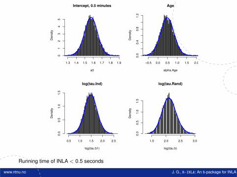
Intercept, 0.5 minutes
a0
De
nsity
1.3 1.4 1.5 1.6 1.7 1.8 1.9
01
23
45
Age
alpha.Age
De
nsity
−0.5 0.0 0.5 1.0 1.5 2.0
0.0
0.4
0.8
1.2
log(tau.Ind)
log(tau.b1)
De
nsity
0.5 1.0 1.5 2.0 2.5
0.0
0.5
1.0
1.5
log(tau.Rand)
log(tau.b)
De
nsity
1.5 2.0 2.5 3.0
0.0
0.5
1.0
1.5
Running time of INLA < 0.5 seconds
www.ntnu.no J. G., R-INLA: An R-package for INLA
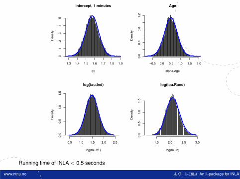
Intercept, 1 minutes
a0
De
nsity
1.3 1.4 1.5 1.6 1.7 1.8 1.9
01
23
45
Age
alpha.Age
De
nsity
−0.5 0.0 0.5 1.0 1.5 2.0
0.0
0.4
0.8
1.2
log(tau.Ind)
log(tau.b1)
De
nsity
0.5 1.0 1.5 2.0 2.5
0.0
0.5
1.0
1.5
log(tau.Rand)
log(tau.b)
De
nsity
1.5 2.0 2.5 3.0
0.0
0.5
1.0
1.5
Running time of INLA < 0.5 seconds
www.ntnu.no J. G., R-INLA: An R-package for INLA
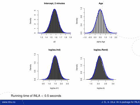
Intercept, 2 minutes
a0
Density
1.3 1.4 1.5 1.6 1.7 1.8 1.9
01
23
45
Age
alpha.Age
Density
−1.0 −0.5 0.0 0.5 1.0 1.5 2.0
0.0
0.4
0.8
1.2
log(tau.Ind)
log(tau.b1)
Density
0.5 1.0 1.5 2.0 2.5
0.0
0.5
1.0
1.5
log(tau.Rand)
log(tau.b)
Density
1.5 2.0 2.5 3.0
0.0
0.5
1.0
1.5
Running time of INLA < 0.5 seconds
www.ntnu.no J. G., R-INLA: An R-package for INLA
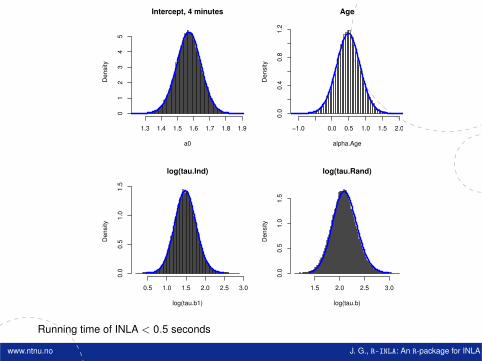
Intercept, 4 minutes
a0
Density
1.3 1.4 1.5 1.6 1.7 1.8 1.9
01
23
45
Age
alpha.Age
Density
−1.0 0.0 0.5 1.0 1.5 2.0
0.0
0.4
0.8
1.2
log(tau.Ind)
log(tau.b1)
Density
0.5 1.0 1.5 2.0 2.5 3.0
0.0
0.5
1.0
1.5
log(tau.Rand)
log(tau.b)
Density
1.5 2.0 2.5 3.0
0.0
0.5
1.0
1.5
Running time of INLA < 0.5 seconds
www.ntnu.no J. G., R-INLA: An R-package for INLA
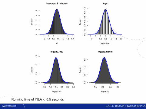
Intercept, 8 minutes
a0
Density
1.3 1.4 1.5 1.6 1.7 1.8 1.9
01
23
45
Age
alpha.Age
Density
−1.0 0.0 0.5 1.0 1.5 2.0
0.0
0.2
0.4
0.6
0.8
1.0
1.2
log(tau.Ind)
log(tau.b1)
Density
0.5 1.0 1.5 2.0 2.5 3.0
0.0
0.5
1.0
1.5
log(tau.Rand)
log(tau.b)
Density
1.5 2.0 2.5 3.0
0.0
0.5
1.0
1.5
Running time of INLA < 0.5 seconds
www.ntnu.no J. G., R-INLA: An R-package for INLA

Intercept, 16 minutes
a0
Density
1.3 1.4 1.5 1.6 1.7 1.8 1.9
01
23
45
Age
alpha.Age
Density
−1.5 −0.5 0.5 1.0 1.5 2.0
0.0
0.2
0.4
0.6
0.8
1.0
log(tau.Ind)
log(tau.b1)
Density
0.5 1.0 1.5 2.0 2.5 3.0
0.0
0.4
0.8
1.2
log(tau.Rand)
log(tau.b)
Density
1.0 1.5 2.0 2.5 3.0
0.0
0.5
1.0
1.5
Running time of INLA < 0.5 seconds
www.ntnu.no J. G., R-INLA: An R-package for INLA
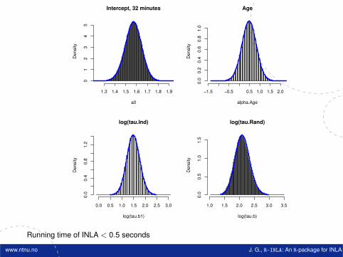
Intercept, 32 minutes
a0
De
nsity
1.3 1.4 1.5 1.6 1.7 1.8 1.9
01
23
45
Age
alpha.Age
De
nsity
−1.5 −0.5 0.5 1.0 1.5 2.0
0.0
0.2
0.4
0.6
0.8
1.0
log(tau.Ind)
log(tau.b1)
De
nsity
0.0 0.5 1.0 1.5 2.0 2.5 3.0
0.0
0.4
0.8
1.2
log(tau.Rand)
log(tau.b)
De
nsity
1.0 1.5 2.0 2.5 3.0 3.5
0.0
0.5
1.0
1.5
Running time of INLA < 0.5 seconds
www.ntnu.no J. G., R-INLA: An R-package for INLA
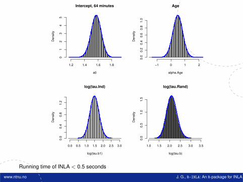
Intercept, 64 minutes
a0
De
nsity
1.2 1.4 1.6 1.8
01
23
45
Age
alpha.Age
De
nsity
−1 0 1 2
0.0
0.2
0.4
0.6
0.8
1.0
log(tau.Ind)
log(tau.b1)
De
nsity
0.0 0.5 1.0 1.5 2.0 2.5 3.0
0.0
0.4
0.8
1.2
log(tau.Rand)
log(tau.b)
De
nsity
1.0 1.5 2.0 2.5 3.0 3.5
0.0
0.5
1.0
1.5
Running time of INLA < 0.5 seconds
www.ntnu.no J. G., R-INLA: An R-package for INLA
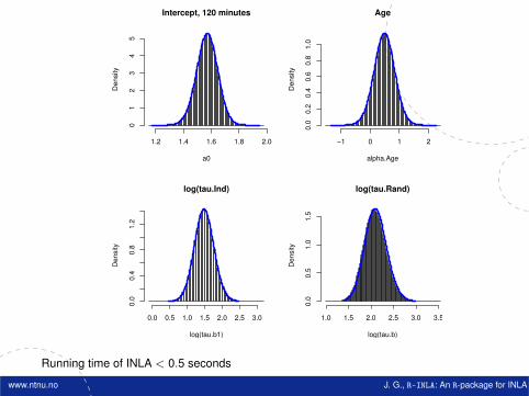
Intercept, 120 minutes
a0
Density
1.2 1.4 1.6 1.8 2.0
01
23
45
Age
alpha.Age
Density
−1 0 1 2
0.0
0.2
0.4
0.6
0.8
1.0
log(tau.Ind)
log(tau.b1)
Density
0.0 0.5 1.0 1.5 2.0 2.5 3.0
0.0
0.4
0.8
1.2
log(tau.Rand)
log(tau.b)
Density
1.0 1.5 2.0 2.5 3.0 3.5
0.0
0.5
1.0
1.5
Running time of INLA < 0.5 seconds
www.ntnu.no J. G., R-INLA: An R-package for INLA
57
Control statementscontrol.xxx statements control computations— control.fixed
• prec: Default precision for all fixed effects except the intercept.prec.intercept: Precision for intercept (Default: 0.0)
— control.family
• link: The link function used in the model if needed.
— control.predictor
• compute: Compute posterior marginals of linear predictors
— control.compute
• dic, mlik, cpo: Compute measures of fit?• config: Save internal GMRF approximations? (needed to useinla.posterior.sample())
— control.inla
• strategy and int.strategy contain useful advanced features
— There are various others as well; see help.
www.ntnu.no J. G., R-INLA: An R-package for INLA
57
Control statementscontrol.xxx statements control computations— control.fixed
• prec: Default precision for all fixed effects except the intercept.prec.intercept: Precision for intercept (Default: 0.0)
— control.family
• link: The link function used in the model if needed.— control.predictor
• compute: Compute posterior marginals of linear predictors
— control.compute
• dic, mlik, cpo: Compute measures of fit?• config: Save internal GMRF approximations? (needed to useinla.posterior.sample())
— control.inla
• strategy and int.strategy contain useful advanced features
— There are various others as well; see help.
www.ntnu.no J. G., R-INLA: An R-package for INLA
57
Control statementscontrol.xxx statements control computations— control.fixed
• prec: Default precision for all fixed effects except the intercept.prec.intercept: Precision for intercept (Default: 0.0)
— control.family• link: The link function used in the model if needed.
— control.predictor
• compute: Compute posterior marginals of linear predictors
— control.compute
• dic, mlik, cpo: Compute measures of fit?• config: Save internal GMRF approximations? (needed to useinla.posterior.sample())
— control.inla
• strategy and int.strategy contain useful advanced features
— There are various others as well; see help.
www.ntnu.no J. G., R-INLA: An R-package for INLA
57
Control statementscontrol.xxx statements control computations— control.fixed
• prec: Default precision for all fixed effects except the intercept.prec.intercept: Precision for intercept (Default: 0.0)
— control.family• link: The link function used in the model if needed.
— control.predictor
• compute: Compute posterior marginals of linear predictors— control.compute
• dic, mlik, cpo: Compute measures of fit?• config: Save internal GMRF approximations? (needed to useinla.posterior.sample())
— control.inla
• strategy and int.strategy contain useful advanced features
— There are various others as well; see help.
www.ntnu.no J. G., R-INLA: An R-package for INLA
57
Control statementscontrol.xxx statements control computations— control.fixed
• prec: Default precision for all fixed effects except the intercept.prec.intercept: Precision for intercept (Default: 0.0)
— control.family• link: The link function used in the model if needed.
— control.predictor• compute: Compute posterior marginals of linear predictors
— control.compute
• dic, mlik, cpo: Compute measures of fit?• config: Save internal GMRF approximations? (needed to useinla.posterior.sample())
— control.inla
• strategy and int.strategy contain useful advanced features
— There are various others as well; see help.
www.ntnu.no J. G., R-INLA: An R-package for INLA
57
Control statementscontrol.xxx statements control computations— control.fixed
• prec: Default precision for all fixed effects except the intercept.prec.intercept: Precision for intercept (Default: 0.0)
— control.family• link: The link function used in the model if needed.
— control.predictor• compute: Compute posterior marginals of linear predictors
— control.compute• dic, mlik, cpo: Compute measures of fit?
• config: Save internal GMRF approximations? (needed to useinla.posterior.sample())
— control.inla
• strategy and int.strategy contain useful advanced features
— There are various others as well; see help.
www.ntnu.no J. G., R-INLA: An R-package for INLA
57
Control statementscontrol.xxx statements control computations— control.fixed
• prec: Default precision for all fixed effects except the intercept.prec.intercept: Precision for intercept (Default: 0.0)
— control.family• link: The link function used in the model if needed.
— control.predictor• compute: Compute posterior marginals of linear predictors
— control.compute• dic, mlik, cpo: Compute measures of fit?• config: Save internal GMRF approximations? (needed to useinla.posterior.sample())
— control.inla
• strategy and int.strategy contain useful advanced features— There are various others as well; see help.
www.ntnu.no J. G., R-INLA: An R-package for INLA
57
Control statementscontrol.xxx statements control computations— control.fixed
• prec: Default precision for all fixed effects except the intercept.prec.intercept: Precision for intercept (Default: 0.0)
— control.family• link: The link function used in the model if needed.
— control.predictor• compute: Compute posterior marginals of linear predictors
— control.compute• dic, mlik, cpo: Compute measures of fit?• config: Save internal GMRF approximations? (needed to useinla.posterior.sample())
— control.inla• strategy and int.strategy contain useful advanced features
— There are various others as well; see help.
www.ntnu.no J. G., R-INLA: An R-package for INLA
57
Control statementscontrol.xxx statements control computations— control.fixed
• prec: Default precision for all fixed effects except the intercept.prec.intercept: Precision for intercept (Default: 0.0)
— control.family• link: The link function used in the model if needed.
— control.predictor• compute: Compute posterior marginals of linear predictors
— control.compute• dic, mlik, cpo: Compute measures of fit?• config: Save internal GMRF approximations? (needed to useinla.posterior.sample())
— control.inla• strategy and int.strategy contain useful advanced features
— There are various others as well; see help.
www.ntnu.no J. G., R-INLA: An R-package for INLA
58
Model choice
There is a need to compare and choose between various models.This is a difficult problem, but R-INLA has some options available:— Marginal likelihood⇒ Bayes factors— Deviance information criterion (DIC)
There are also some predictive checks for the model:— Conditional predictive ordinate (CPO)— Probability integral transform (PIT)
www.ntnu.no J. G., R-INLA: An R-package for INLA
59
Marginal likelihood
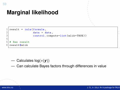
1 result = inla(formula ,2 data = data ,3 control.compute=list(mlik=TRUE))45 # See result6 result$mlik
— Calculates log(π(y))— Can calculate Bayes factors through differences in value
www.ntnu.no J. G., R-INLA: An R-package for INLA
60
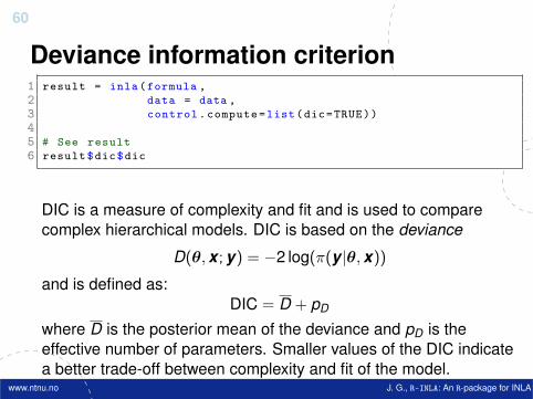
Deviance information criterion1 result = inla(formula ,2 data = data ,3 control.compute=list(dic=TRUE))45 # See result6 result$dic$dic
DIC is a measure of complexity and fit and is used to comparecomplex hierarchical models. DIC is based on the deviance
D(θ,x ;y) = −2 log(π(y |θ,x))and is defined as:
DIC = D + pD
where D is the posterior mean of the deviance and pD is theeffective number of parameters. Smaller values of the DIC indicatea better trade-off between complexity and fit of the model.
www.ntnu.no J. G., R-INLA: An R-package for INLA
61
Conditional predictive ordinate
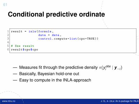
1 result = inla(formula ,2 data = data ,3 control.compute=list(cpo=TRUE))45 # See result6 result$cpo$cpo
— Measures fit through the predictive density π(yobsi | y−i)
— Basically, Bayesian hold-one out— Easy to compute in the INLA-approach
www.ntnu.no J. G., R-INLA: An R-package for INLA
62
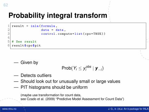
Probability integral transform1 result = inla(formula ,2 data = data ,3 control.compute=list(cpo=TRUE))45 # See result6 result$cpo$pit
— Given byProb(Yi ≤ yobs
i | y−i)
— Detects outliers— Should look out for unusually small or large values— PIT histograms should be uniform
(maybe use transformation for count data,see Czado et al. (2009) “Predictive Model Assessment for Count Data”)
www.ntnu.no J. G., R-INLA: An R-package for INLA
63
Useful features
There are several features that can be used to extend the standardmodels in R-INLA
— Replicate and group— Multiple likelihoods— Copy— Linear transformation of linear predictor (A matrix)— Linear combinations— Remote computing
www.ntnu.no J. G., R-INLA: An R-package for INLA
64
Feature: replicate
“replicate” generates iid replicates from the same f()-model withthe same hyperparameters.
If x | θ ∼ AR(1), then nrep=3, makes
x = (x1,x2,x3)
with mutually independent x i ’s from AR(1) with the same θArguments
f(..., replicate = r [, nrep = nr ])
where replicate are integers 1,2, . . . , etc
www.ntnu.no J. G., R-INLA: An R-package for INLA
65
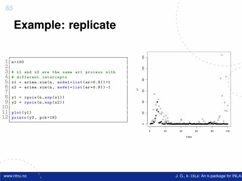
Example: replicate
1 n=10023 # x1 and x2 are the same ar1 process with4 # different intercepts5 x1 = arima.sim(n, model=list(ar =0.9))+16 x2 = arima.sim(n, model=list(ar =0.9)) -178 y1 = rpois(n,exp(x1))9 y2 = rpois(n,exp(x2))
1011 plot(y1)12 points(y2, pch =19}
0 20 40 60 80 100
020
40
60
80
100
12
0
Indexy1
www.ntnu.no J. G., R-INLA: An R-package for INLA
66
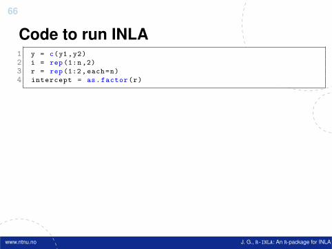
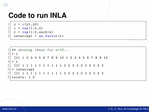
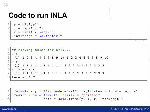
Code to run INLA1 y = c(y1,y2)2 i = rep(1:n,2)3 r = rep(1:2, each=n)4 intercept = as.factor(r)
1 ## showing these for n=10...2 > i3 [1] 1 2 3 4 5 6 7 8 9 10 1 2 3 4 5 6 7 8 9 104 > r5 [1] 1 1 1 1 1 1 1 1 1 1 2 2 2 2 2 2 2 2 2 26 > intercept7 [1] 1 1 1 1 1 1 1 1 1 1 2 2 2 2 2 2 2 2 2 28 Levels: 1 2
1 formula = y ~ f(i, model="ar1", replicate=r) + intercept -12 result = inla(formula , family = "poisson",3 data = data.frame(y, i, r, intercept))
www.ntnu.no J. G., R-INLA: An R-package for INLA
66
Code to run INLA1 y = c(y1,y2)2 i = rep(1:n,2)3 r = rep(1:2, each=n)4 intercept = as.factor(r)
1 ## showing these for n=10...2 > i3 [1] 1 2 3 4 5 6 7 8 9 10 1 2 3 4 5 6 7 8 9 104 > r5 [1] 1 1 1 1 1 1 1 1 1 1 2 2 2 2 2 2 2 2 2 26 > intercept7 [1] 1 1 1 1 1 1 1 1 1 1 2 2 2 2 2 2 2 2 2 28 Levels: 1 2
1 formula = y ~ f(i, model="ar1", replicate=r) + intercept -12 result = inla(formula , family = "poisson",3 data = data.frame(y, i, r, intercept))
www.ntnu.no J. G., R-INLA: An R-package for INLA
67
Feature: group
— Similar concept as replicate, but with a dependence structureon the replicates. E.g. rw1, rw2, ar1, exchangeable
— Implemented as a Kronecker product (often space and time)— It’s possible to use both replicate and group! This will be
replications of the grouped model— Used with f(..., group = g [, ngroup = ng])
www.ntnu.no J. G., R-INLA: An R-package for INLA
68
Feature: multiple likelihoods
In many situations, you need to combine data from differentsources and need to be able to handle multiple likelihoods.
Examples:— Joint modelling of longitudinal and event time data
(Guo and Carlin, 2004)— “Marked” point processes— Combining data from multiple experiments
www.ntnu.no J. G., R-INLA: An R-package for INLA
69
Feature: multiple likelihoods
— We can have different likelihoods, either through differentfamilies or the same family with different parameters. E.g. jointmodelling of two species (probably) needs differentparameters for the distributions of the responses.
— The response y is a matrix (or list) where a different “family” isapplied to each column
— Each “family” introduces new hyperparameters
www.ntnu.no J. G., R-INLA: An R-package for INLA
70
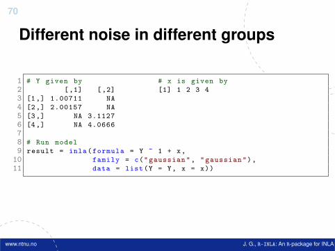
Different noise in different groups
1 # Y given by # x is given by2 [,1] [,2] [1] 1 2 3 43 [1,] 1.00711 NA4 [2,] 2.00157 NA5 [3,] NA 3.11276 [4,] NA 4.066678 # Run model9 result = inla(formula = Y ~ 1 + x,
10 family = c("gaussian", "gaussian"),11 data = list(Y = Y, x = x))
www.ntnu.no J. G., R-INLA: An R-package for INLA
71
Feature: copy
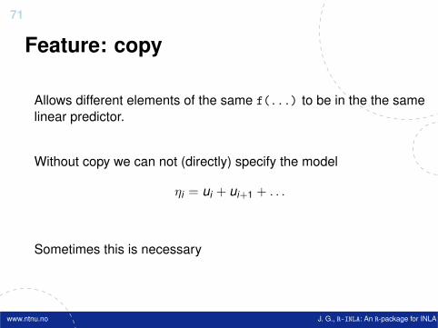
Allows different elements of the same f(...) to be in the the samelinear predictor.
Without copy we can not (directly) specify the model
ηi = ui + ui+1 + . . .
Sometimes this is necessary
www.ntnu.no J. G., R-INLA: An R-package for INLA
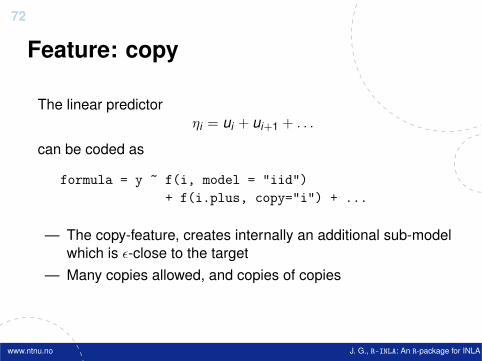
72
Feature: copy
The linear predictorηi = ui + ui+1 + . . .
can be coded as
formula = y ~ f(i, model = "iid")+ f(i.plus, copy="i") + ...
— The copy-feature, creates internally an additional sub-modelwhich is ε-close to the target
— Many copies allowed, and copies of copies
www.ntnu.no J. G., R-INLA: An R-package for INLA
73
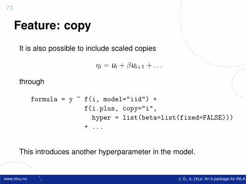
Feature: copy
It is also possible to include scaled copies
ηi = ui + βui+1 + . . .
through
formula = y ~ f(i, model="iid") +f(i.plus, copy="i",
hyper = list(beta=list(fixed=FALSE)))+ ...
This introduces another hyperparameter in the model.
www.ntnu.no J. G., R-INLA: An R-package for INLA
74
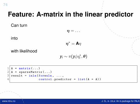
Feature: A-matrix in the linear predictorCan turn
η = . . .
intoη∗ = Aη
with likelihoodyi ∼ π(yi |η∗i ,θ)
1 A = matrix (...)2 A = sparseMatrix (...)3 result = inla(formula , ...,4 control.predictor = list(A = A))
www.ntnu.no J. G., R-INLA: An R-package for INLA
75
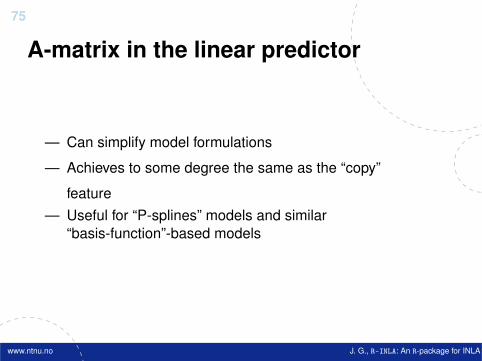
A-matrix in the linear predictor
— Can simplify model formulations
— Achieves to some degree the same as the “copy”
feature— Useful for “P-splines” models and similar
“basis-function”-based models
www.ntnu.no J. G., R-INLA: An R-package for INLA
76
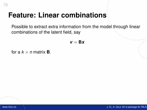
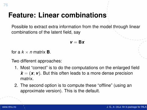
Feature: Linear combinationsPossible to extract extra information from the model through linearcombinations of the latent field, say
v = Bx
for a k × n matrix B.
Two different approaches:1. Most “correct” is to do the computations on the enlarged field
x̃ = (x ;v). But this often leads to a more dense precisionmatrix.
2. The second option is to compute these “offline” (using anapproximate version). This is the default.
www.ntnu.no J. G., R-INLA: An R-package for INLA
76
Feature: Linear combinationsPossible to extract extra information from the model through linearcombinations of the latent field, say
v = Bx
for a k × n matrix B.
Two different approaches:1. Most “correct” is to do the computations on the enlarged field
x̃ = (x ;v). But this often leads to a more dense precisionmatrix.
2. The second option is to compute these “offline” (using anapproximate version). This is the default.
www.ntnu.no J. G., R-INLA: An R-package for INLA
77
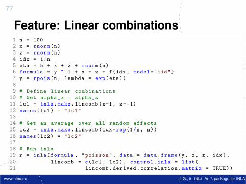
Feature: Linear combinations1 n = 1002 x = rnorm(n)3 z = rnorm(n)4 idx = 1:n5 eta = 5 + x + z + rnorm(n)6 formula = y ~ 1 + x + z + f(idx , model="iid")7 y = rpois(n, lambda = exp(eta))89 # Define linear combinations
10 # Get alpha_x - alpha_z11 lc1 = inla.make.lincomb(x=1, z=-1)12 names(lc1) = "lc1"1314 # Get an average over all random effects15 lc2 = inla.make.lincomb(idx=rep(1/n, n))16 names(lc2) = "lc2"1718 # Run inla19 r = inla(formula , "poisson", data = data.frame(y, x, z, idx),20 lincomb = c(lc1 , lc2), control.inla = list(21 lincomb.derived.correlation.matrix = TRUE))
www.ntnu.no J. G., R-INLA: An R-package for INLA
78
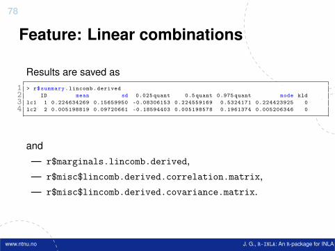
Feature: Linear combinations
Results are saved as1 > r$summary.lincomb.derived2 ID mean sd 0.025 quant 0.5 quant 0.975 quant mode kld3 lc1 1 0.224634269 0.15659950 -0.08306153 0.224559169 0.5324171 0.224423925 04 lc2 2 0.005198819 0.09720661 -0.18594403 0.005198578 0.1961374 0.005206346 0
and— r$marginals.lincomb.derived,— r$misc$lincomb.derived.correlation.matrix,— r$misc$lincomb.derived.covariance.matrix.
www.ntnu.no J. G., R-INLA: An R-package for INLA
79
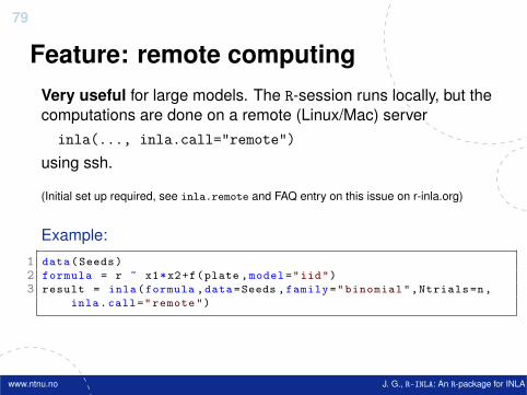
Feature: remote computingVery useful for large models. The R-session runs locally, but thecomputations are done on a remote (Linux/Mac) server
inla(..., inla.call="remote")
using ssh.
(Initial set up required, see inla.remote and FAQ entry on this issue on r-inla.org)
Example:
1 data(Seeds)2 formula = r ~ x1*x2+f(plate ,model="iid")3 result = inla(formula ,data=Seeds ,family="binomial",Ntrials=n,
inla.call="remote")
www.ntnu.no J. G., R-INLA: An R-package for INLA
80
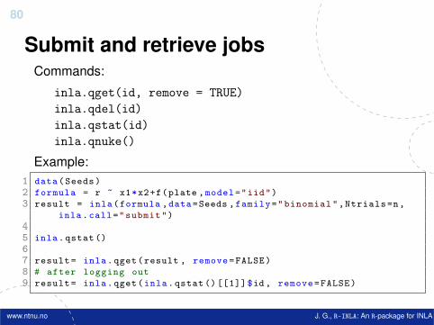
Submit and retrieve jobsCommands:
inla.qget(id, remove = TRUE)inla.qdel(id)inla.qstat(id)inla.qnuke()
Example:1 data(Seeds)2 formula = r ~ x1*x2+f(plate ,model="iid")3 result = inla(formula ,data=Seeds ,family="binomial",Ntrials=n,
inla.call="submit")45 inla.qstat()67 result= inla.qget(result , remove=FALSE)8 # after logging out9 result= inla.qget(inla.qstat ()[[1]]$id , remove=FALSE)
www.ntnu.no J. G., R-INLA: An R-package for INLA
81
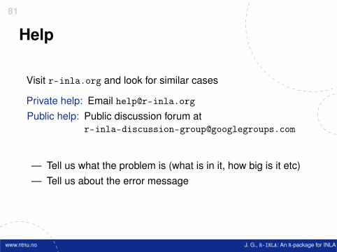
Help
Visit r-inla.org and look for similar cases
Private help: Email [email protected] help: Public discussion forum at
— Tell us what the problem is (what is in it, how big is it etc)— Tell us about the error message
www.ntnu.no J. G., R-INLA: An R-package for INLA
82
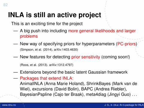
INLA is still an active projectThis is an exciting time for the project
— A big push into including more general likelihoods and largerproblems
— New way of specifying priors for hyperparameters (PC-priors)(Simpson, et al. (2014), arXiv:1403.4630)
— New features for detecting prior sensitivity (coming soon!)
(Roos, et al. (2013). arXiv:1312.4797)
— Extensions beyond the basic latent Gaussian framework— Packages that extend INLA:
AnimalINLA (Anna Marie Holand), ShrinkBayes (Mark van deWiel), excursions (David Bolin), BAPC (Andrea Riebler),BayesianPspline (Cajo ter Braak), meta4diag (Jingyi Guo) . . .
www.ntnu.no J. G., R-INLA: An R-package for INLA

83
Thank you for your attention!
If you have any questions, please write me:[email protected]
r-in
la.o
rg
@le
g.uf
pr.b
r
INLA
MU
G inla(formula, family, control.family=list(hyper, ...), control.mix=list(hyper, ...),data, E, offset, scale, weights, Ntrials, strata, link.covariates, lincomb,
control.fixed, control.predictor, control.compute, control.inla, control.hazard, ...)
y ~ fix.eff + f(i, model, control.group=list(model, ...), hyper, ...)
beta, (|g)poisson, (|circular|skew|log)normal, t,(|beta|c)binomial, coxph, laplace, weibull(|cure),log(gammafrailty|istic|logistic|periodogram), gev,zeroinflated(poisson|(|beta|n)binomial)[0-2], ...
(|c)linear, iid, iid[1-5]d, me(c|b), copy, z,(|rev)sigm, ar(|1), rw[1-2], crw2, seasonal,ou, besag(|2|proper|proper2), bym(|2), slm,generic(|[0-3]), rgeneric, spde[1-3], ...
rw[1-2],ar(|1),besag,exchang.
loggamma, wishart[1-4]d, table:,pc.prec, pc.dof, expression:, ...
rw1, rw2
list(mean,prec,...)
list(A,compute,cross,link, ...)
list(mlik,dic, waic,cpo, po,config, ...)
list(strategy=c("simplified.laplace", "gaussian","laplace"), int.strategy=c("ccd","grid","eb"),h, dz, tolerance, optimizer, npoints, stencil,diagonal, step.factor, correct.strategy, ...)
list(hyper,
model,...)
1
www.ntnu.no J. G., R-INLA: An R-package for INLA


