Robust control of identi�ed models with mixed parametric and

non-parametric uncertainties

Wolfgang Reinelt and Lennart Ljung

Department of Electrical Engineering

Link �oping University, S-581 83 Link �oping, Sweden

WWW: http://www.control.isy.liu.se/

Email: {wolle,ljung}@isy.liu.se

November 27, 2000

REGLERTEKNIK

AUTOMATIC CONTROL

LINKÖPING

Report no.: LiTH-ISY-R-2319

Submitted to: European Control Conference 2001, Porto, Portugal

Technical reports from the Automatic Control group in Link �oping are available by anonymous ftp at

the address ftp.control.isy.liu.se. This report is contained in the portable document format �le

2319.pdf.

Robust control of identi�ed models with mixed

parametric and non-parametric uncertainties∗

Wolfgang Reinelt† and Lennart Ljung

Dept of Electrical Engineering, Link �oping University, 581 83 Link �oping, Sweden,{wolle,ljung}@isy.liu.se, http://www.control.isy.liu.se

Phone: +46-13-281333, Telefax: +46-13-282622

Abstract

A straightforward framework for identi�cation oriented robust controller design is presented.

The model set, directly identi�ed from data, is based on model error modeling and model validation

techniques. The set of all robustly stabilizing controllers, that additionally guarantee robust per-

formance, is characterized by a system of second order cones, which can be eÆciently solved using

interior point algorithms. We illustrate the proposed method and the choice of the parameters with

an example. Moreover, the interplay between identi�cation and controller design can be analyzed

in this framework.

Keywords: Identi�cation for Control, Model ErrorModeling, Robust Stability and Performance, Rank

One Uncertainties.

Submitted to the European Control Conference 2001, Porto, Portugal, as a regular paper for presen-

tation in a lecture session.

Topics:

1. System identi�cation and signal processing: Identi�cation for control

4. Design methodologies: Robust control

∗Financial support in part by the European Commission through the programTraining andMobility of Researchers - Research

Networks and through the project System Identi�cation (FMRX CT98 0206) and contacts with the participants in the European

Research Network System Identi�cation (ERNSI) are gratefully acknowled ged.†Corresponding author.

1

1 Introduction and Motivation

Much of current interest in System Identi�cation is dedicated to Control Oriented Identi�cation or

Identi�cation for Control, see [6, 9, 16] and the references therein. The gap to bridge between

identi�cation and control is the model uncertainty, which will be addressed by a robust controller.

More speci�cally, the interplay between the model builder (MB) and the control designer (CD) can

be described as follows [10]:

1. The MB computes a set of models, using measured data. This model set usually contains a

nominal model: the MB thinks that this model explains the data best (from the knowledge

gained from data). The model uncertainty or error is explained by the model set. The rationale

used for producing this model set is immaterial in this context.

2. Based on nominal model and model set, the CD constructs a robust controller, that also gives

acceptable closed loop performance. Typically, performance speci�cations are given by someone

else than CD or MB, and maybe negotiable.

3. The constructed controller is tested on the real plant, that was used for collecting the data.

The scheme seems simple, but is by no means without interaction between the three steps. The most

interesting situation is when the \real life test" in step 3 fails. The question arising then is: what

do we have to improve, in order to obtain a better result? Moreover, we are facing the fundamental

robustness vs. performance tradeo�:

• Emphasizing robustness: suppose, the model set identi�ed by MB is too inaccurate to describe

the real world (i.e. the real plant is outside the model set). Then it has to be modi�ed, made

larger, to include the real plant. A crucial point is, that the model set should not grow too much,

because then it is more likely that the controller will be conservative.

• Emphasizing performance: it may be too diÆcult or impossible to design a robust controller on

the delivered model set, ful�lling the speci�cations. The controller is too conservative. If we

cannot step back from these speci�cations, the model set has to be modi�ed: made smaller or

\more accurate". While decreasing the model set, the real plant should still be included in the

set.

Whatever we have to emphasize, robustness or performance, the model set has to be modi�ed. A

question is, whether this can be done without collecting new data or not? Moreover, the MB wants

to have some information from the CD, where (i.e. in which frequency range) the model has to be

modi�ed.

Related Works and Our Contribution

The problem of controller validation for stability and performance for an identi�ed model set is well

understood by now [2, 3]. Still, there is a lack of actual design techniques, directly based on recent

identi�cation techniques that deliver a nominal model along with an uncertainty region. This work

is intended to attack this gap from the control point of view.

Mainstream works on robust control focus mainly on unstructured uncertainties and are therefore

not always suited for model sets, obtained from identi�cation procedures. However, necessary and

suÆcient results on robust stability for rank one uncertainties are given is [14]. There, the set of all

controllers is parameterized using Youla parameterization.

A somewhat related question is studied in [12], where interval arithmetic is applied to analyze

model sets that depend nonlinearly on some uncertain parameters. The construction of the set of

all feasible controllers however, is computationally demanding and therefor restricted to small-sized

problems. Moreover, the straightforward identi�cation of such models directly from data is a diÆcult

task and so far unsolved.

We will present a framework which starts with identi�cation of a model set, describing the under-

lying dataset. The employed identi�cation procedure relates strongly to our previous works on model

error modeling and model validation techniques [10, 5, 15]. The remaining task is to design a robust

controller, that guarantees stabilization of the model set. Our contributions are the following:

1

• Robust stabilization of a set of (identi�ed) models, containing real parametric uncertainties as

well as non-parametric, dynamical model error models. In contrast to the result obtained in

[7], we will use the \correct" norm (the one we use in the identi�cation step) and also allow an

explicit, non-parametric model error model.

• Performance requirements: Robust sensitivity can be prescribed in standard H∞ terminology

and, moreover, the sensitivity function of the nominal control system can be prescribed within

certain (sharper) frequency-bounds.

• Formulation of the robust stability and performance problem as second order cone programming

problem. Being a special case of the \standard" semide�nite programming problem, it enables

an eÆcient numerical solution.

• We provide an explicit recommendation for the choice of the basis functions, parameterizing the

Youla parameter (and so the controller).

Paper Outline: Section 2 summarizes short the result of a control-oriented identi�cation procedure,

while Section 3 then discusses controller design ensuring robust stability as well as guaranteeing a

certain robust performance. An example in Section 4 illustrates the presented framework and Section 5

gives some comments and suggests possibilities of future work.

2 What the Identi�cation procedure delivers

We consider two identi�cation methods, that allow a parameterization of the underlying model class

in terms of orthonormal basis functions:

1. Least Squares Estimation using basis functions. Here, the data might be pointwise transfer

function estimates from time domain data or direct measurements in the frequency domain.

2. Set membership estimation, assuming an unknown-but-bounded (UBB) noise using time- or

frequency-domain data.

In both cases, we end up with a set of single-input single-output models of the following structure:

G(iω, θ) = B(iω)θ with (1)

(θ − θnom)TE−1(θ − θnom) ≤ ρ (2)

Gnom(iω) = G(iω, θnom) = B(iω)θnom (3)

Here B denotes the vector of chosen basis functions, θ the vector of admissible parameters, located

in the ellipsoid described by the positive de�nite matrix E. Gnom is the nominal model and

Us := {G(iω, θ), θ ful�lls eqn. (2)} (4)

is the model set (explaining the data). Applying set membership techniques, the matrix E in eqn. (2)

refers to the ellipsoid, calculated when using and ellipsoid algorithm and ρ = 1. Using Least Squares

methods, E is the covariance matrix of the parameter and ρ is linked to the probability level of the

estimation.

In recent works [10, 5, 15] we emphasized that is advantageous to employ an unfalsi�ed and

explicit model error model to cope with unmodeled dynamics, nonlinearities, time varying drifts etc.

The result of such an identi�cation is then

G∆(iω) = Gnom(iω) +W∆(iω)∆(iω) with (5)

||∆||∞ ≤ 1. (6)

The model error model will typically come along with a shaping weight W∆ for normalization pur-

poses. The model set explaining the data will then be

Uus := {G∆(iω) = Gnom(iω) +W∆(iω)∆(iω), ∆ ful�lls eqn. (6)} (7)

2

�∆

K

P

w z

yu

Figure 1: Generalized plant P with uncertainty �∆ and controller K in an LFT framework.

Clearly, both model uncertainties discussed so far are of di�erent nature: the model set Us givenby eqn. (4) is represented by a real parametric uncertainty, bounded in 2-norm, while the model set

Uus given by eqn. (7) represents a non-parametric uncertainty, bounded in∞-norm. It may be useful

to combine both types of uncertainty set to cope with uncertainties in the parameters of the nominal

model as well as with unmodeled dynamics, which leads to the following model set

U := {G(iω) = G(iω, θ) +W∆(iω)∆(iω), θ ful�lls eqn. (2) and ∆ ful�lls eqn. (6)} (8)

In this context, G(θnom) will be the nominal model.

3 Controller Design

3.1 Robust Stability and Performance

Clearly, the model set as described in eqns. (8) �ts to standard uncertainty descriptions (cf. �g. 1),

when resorting the two contributions of uncertainty to �∆. Therefore it is possible to use well es-

tablished control schemes like mixed sensitivity H∞ control, taking the uncertainty band in the fre-

quency domain in account for the robust controller design. As we are facing a structured uncertainty,

we can do better using µ techniques, i.e. use K-D iteration for controller design. But here, we are

in a much more speci�c situation: the uncertainty �∆, as depicted in �g. 1, consists, as discussed

above, of two parts: the real uncertainty vector δ is situated in the ellipsoid given in eqn. (2). There-

fore, the uncertainty is given in the 2-norm: ||δ||2 ≤ 1, which is obvious from eqn. (2), denoting

δ = 1√ρT(θ− θnom), T · T = E−1. The nonparametric uncertainty is bounded in operator (H∞ ) norm by

1.

Thus, the model set delivered by identi�cation �ts to the framework of �g. 1 with rank one uncer-

tainty (δT , ∆) and a generalized plant P, that is known from the identi�cation procedure:

P(iω) =

0

( √ρ T−TBT (iω)

W∆(iω)

)1 Gnom(iω)

.Additionally to robust stability, we ask the controller to guarantee certain performance speci�cations

for the identi�ed model set (8). In particular we demand an upper bound WS for the sensitivity

function S:

||W−1S · S(δT , ∆)||∞ ≤ 1, ∀||δ||2 ≤ 1, ||∆||∞ ≤ 1,

which is equivalent to robust stability by adding a dummy uncertainty ∆S to the uncertainty vector

3

and applying the small gain theorem. The above setup then reads as

P(iω) =

0

0

WS(iω)−1

√ρ T−TBT (iω)

W∆(iω)

WS(iω)−1Gnom(iω)

1 Gnom(iω)

, (9)

(z

y

)= P(iω) ·

(w

u

), (10)

w = �∆z = (δT , ∆, ∆S)z, ||δ||2 ≤ 1, ||∆||∞ ≤ 1, ||∆S||∞ ≤ 1. (11)

We now use the convex parameterization of all stabilizing controllers, as given in [14] to construct

a robust controller. Suppose, we have a Youla parameterization1 of the nominal i/o behavior from

w to z: T1 + T2Q, where Q is the Youla parameter. Assume moreover a decomposition of (T1, T2)

corresponding to the uncertain vector (δT , ∆, ∆S)T :

(T1, T2) =

Tδ1 Tδ2T∆1 T∆2T∆S1 T

∆S2

.Robust stability for the feedback loop is now to demand:

[1− (δT , ∆, ∆S)(T1 + T2Q)]−1 ∈ H∞ , ∀ δ, ∆,∆S (12)

A rather elegant and computational attractive solution to this robust stability problem is given by the

following:

3.1 Theorem (Rantzer and Megretski, 1994 [14, Cor.2]): Under the assumptions described so far,

eqn.(12) is equivalent to the existence of two stable functions α,β (of appropriate dimension) with

Q = β/α ful�lling

||Re[Tδ1α+ Tδ2β](iω)||d + ||(T∆1 α+ T∆2 β)(iω)||2 + ||(T∆S1 α+ T∆S2 β)(iω)||2 < Reα(iω), ∀ ω (13)

where || · ||d is denotes the dual norm to || · ||.

3.2 Remark: The original Theorem [14, Cor.2] is stated for one dynamical uncertainty, i.e. ∆S = in

the above setup. However, it is straightforward to verify the above \extended" version.

3.3 Remark: The remaining problem is to �nd the two functions α,β in the now convex setting of

eqn. (13). In [7], this problem is solved for a parametric uncertainty (i.e. T∆1 , T∆2 , T

∆S1 , T∆S2 = 0)

bounded in 1-norm and∞-norm respectively using an FIR basis for the two functions in question and

the computational problem is recasted to a linear programming one.

Several aspects require to abandon the existing (numerical) solution of Theorem 3.1, mentioned

in the remark above. Apart from the missing dynamical error/explicit model error model and the

performance speci�cation, in our case, the uncertainty is bounded in the 2-norm, so that || · ||d =

|| · || = || · ||2. Moreover it turns out that a more exible parameterization of the two functions α,β is

of advantage. Hence we will assume a more general orthonormal basis:

α = Bαθα, β = Bβθβ (14)

of dimension Nα and Nβ respectively, i.e. θα ∈ IRNα and θβ ∈ IRNβ. Obviously, eqn. (13) is then

(assuming in�nite basis expansion, i.e. Nα, Nβ →∞) equivalent to

||Rsθ||2 + ||Rusθ||2 + ||RPθ||2 < RTmθ ∀ω (15)

1the general term T12QT21 boils down to T2Q, becausew is a scalar signal.

4

denoting θT = (θTα, θTβ) and (the dependence on frequency ω being suppressed):

Rs = (ReTδ1Bα, ReTδ2Bβ), Rus =

(ReT∆1 Bα ReT∆2 BβImT∆1 Bα ImT∆2 Bβ

), RP =

(ReT

∆S1 Bα ReT

∆S2 Bβ

ImT∆S1 Bα ImT∆S2 Bβ

), Rm = ReBTα

Eqn. (15) is equivalent to the following Second-order Cone Problem [11], when introducing three

additional dummy-variables, i.e. ~θ = (θT , ζ1, ζ2, ζ3)T :

0 < ~RTm ~θ (16)

|| ~Rs ~θ||2 ≤ (0, 1, 0, 0) ~θ (17)

|| ~Rus ~θ||2 ≤ (0, 0, 1, 0) ~θ (18)

|| ~RP ~θ||2 ≤ (0, 0, 0, 1) ~θ (19)

Here, 0 denotes the row vector with Nα + Nβ zero entries and some obvious zero block have been

added to the previous matrices:

~Rs = (Rs, 0, 0, 0), ~Rus = (Rus, 0, 0, 0), ~RP = (RP, 0, 0, 0), ~Rm = (RTm,−1,−1,−1)T .

This problem can be solved quite eÆciently with standard software as SOCP, see [11].

3.2 Imposing additional (sharper) Nominal Performance

The previous section treats the robust stability and performance problem. In the particular situa-

tion, that identi�cation is performed using a set of stable basis functions, demanding performance

additionally to stability avoids the trivial solution (i.e. zero controller).

Moreover, it is rather easy in the case to impose additional demands on the sensitivity function of

the nominal control system, which is in then S = I −GnomQ. Motivation for this may be to demand

sharper performance in the nominal case (which is supposed to be the \most likely" one) and weaker

performance in the disturbed case. Assuming a lower and an upper bound Slo(iω), Shi(iω) (both

assumed to be non-negative) for the sensitivity, this is

|Slo(iω)α(iω)| ≤ |α(iω) −Gnom(iω)β(iω)| ≤ |Shi(iω)α(iω)|, ∀ω. (20)

Reformulation in terms of basis functions gives the following system of equations:

||Slo(iω)Sα(iω)θα||2 ≤∣∣∣∣∣∣∣∣S(iω)

(θαθβ

)∣∣∣∣∣∣∣∣2

≤ ||Shi(iω)Sα(iω)θα||2 , ∀ω, (21)

where (the dependence on ω being suppressed as above):

Sα =

(ReBαImBα

), S =

(ReBα −ReGnomBβImBα −ImGnomBβ

)For consistency with the variable ~θ = (θTα, θ

Tβ, ζ1, ζ2)

T from above, we add obvious zero blocks to

matrices Sα,S and obtain and equivalent formulation of eqn. (21):∣∣∣∣Slo ~Sα ~θ∣∣∣∣2 ≤ ∣∣∣∣ ~S ~θ∣∣∣∣2 ≤ ∣∣∣∣Shi ~Sα ~θ∣∣∣∣2 . (22)

For easier argumentation, we break the inequality into four inequalities (for a moment)∣∣∣∣Slo ~Sα ~θ∣∣∣∣2 ≤ γlo (23)

γlo ≤∣∣∣∣ ~S ~θ∣∣∣∣

2(24)∣∣∣∣ ~S ~θ∣∣∣∣

2≤ γhi (25)

γhi ≤∣∣∣∣Shi ~Sα ~θ∣∣∣∣2 , (26)

5

which have to hold for all frequencies. Following the same argumentation as in the previous section,

inequalities (23) and (25) form convex conditions and can be written as SOCPs, whereas inequali-

ties (24) and (26) are non-convex. Inequality (21), however, can be scaled in θα, θβ, so that it is

equivalent to demand that one of the components of the vectors ~S ~θ and Shi ~Sα ~θ has to have at least

the demanded size γlo and γhi respectively. All this leads to∣∣∣∣Slo ~Sα ~θ∣∣∣∣2 ≤ ~S · ej · ~θ (27)∣∣∣∣ ~S ~θ∣∣∣∣2≤ Shi ~Sα · ek · ~θ (28)

denoting el the l − th unit vector. Conditions (27) and (28) are second order cones and can easily be

added to the minimization problem from above.

3.3 Controller design as second order cone feasibility problem

Imposing robust stability as well as nominal performance properties, the set of feasible solutions to

the control problem is given by restrictions (16,17,18,19,27,28), which build up a convex cone for the

variable ~θ = (θTα, θTβ, ζ1, ζ2, ζ3)

T :

0 < ~RTm ~θ (29)

|| ~Rs ~θ||2 ≤ (0, 1, 0, 0) ~θ ⇔ ((0, 1, 0, 0) ~θ ( ~Rs ~θ)T

~Rs ~θ (0, 1, 0, 0) ~θ · I

)> 0 (30)

|| ~Rus ~θ||2 ≤ (0, 0, 1, 0) ~θ ⇔ ((0, 0, 1, 0) ~θ ( ~Rus ~θ)T

~Rus ~θ (0, 0, 1, 0) ~θ · I

)> 0 (31)

|| ~RP ~θ||2 ≤ (0, 0, 0, 1) ~θ ⇔ ((0, 0, 0, 1) ~θ ( ~RP ~θ)T

~RP ~θ (0, 0, 0, 1) ~θ · I

)> 0 (32)

∣∣∣∣Slo ~Sα ~θ∣∣∣∣2 ≤ ~S · ej · ~θ ⇔ (~S ~θ · ej (Slo ~Sα ~θ)TSlo ~Sα ~θ ~S ~θ · ej · I

)≥ 0 (33)

∣∣∣∣ ~S ~θ∣∣∣∣2≤ Shi ~Sα · ek · ~θ ⇔ (

Shi ~Sα ~θ · ek ( ~S ~θ)T~S ~θ Shi ~Sα ~θ · ek · I

)≥ 0 (34)

We remark, that the numerical solution of the problem using second order cones conditions (left

column in the above system of inequalities) instead of the equivalent standard LMI system (right

column) is of advantage.

Special cases of the design problem obviously arise when no parametric uncertainty or no explicit

model error model is present: ~Rs = 0 and ~Rus = 0 in eqns.(30,31) respectively. RS = 0 in eqn.(32)

imposes no further demands on robust sensitivity. Moreover Slo = 0 and 1/Shi = 0 in eqns.(33,34)

respectively indicate absence of a lower and upper bound for nominal sensitivity.

3.4 Choice of the basis functions

A �nal remark can be made on the choice of the basis functions Bα. Eqn. (13) implies strict positive

realness of the function α, which is easy seen from letting ρ = 0. Suppose, we have a state space

representation of Bαz= (A,B,C,D). Then, the discrete time version of the positive real lemma [8,

problem 3.25] (using the bilinear transformation z = (1 + s)/(1 − s) to derive it from the continuous

time version, cf. [8, problem 4.18]) states, that a necessary condition for this is

[D− C(I +A)−1B] + [(D − C(I +A)−1B]T > 0.

In the SISO case, this will be equivalent with D− C(I+ A)−1B > 0.

Suppose as an simple example the �rst order Laguerre basis with pole at −1 < a < 1: Bαz=

(a, 1,√

(1− a2), 0), then α(z)z= (a, 1,

√(1− a2)θα, 0) for some scalar parameter θα. The above neces-

sary condition for strict positive realness is then θα

√1−a1+a

< 0, which implies θα < 0. Additionally,

6

10−2

10−1

100

101

102

10−4

10−3

10−2

10−1

100

101

Frequency

Mag

nitu

de

Nominal model (b−) with uncertainty region and real plant (r−−)

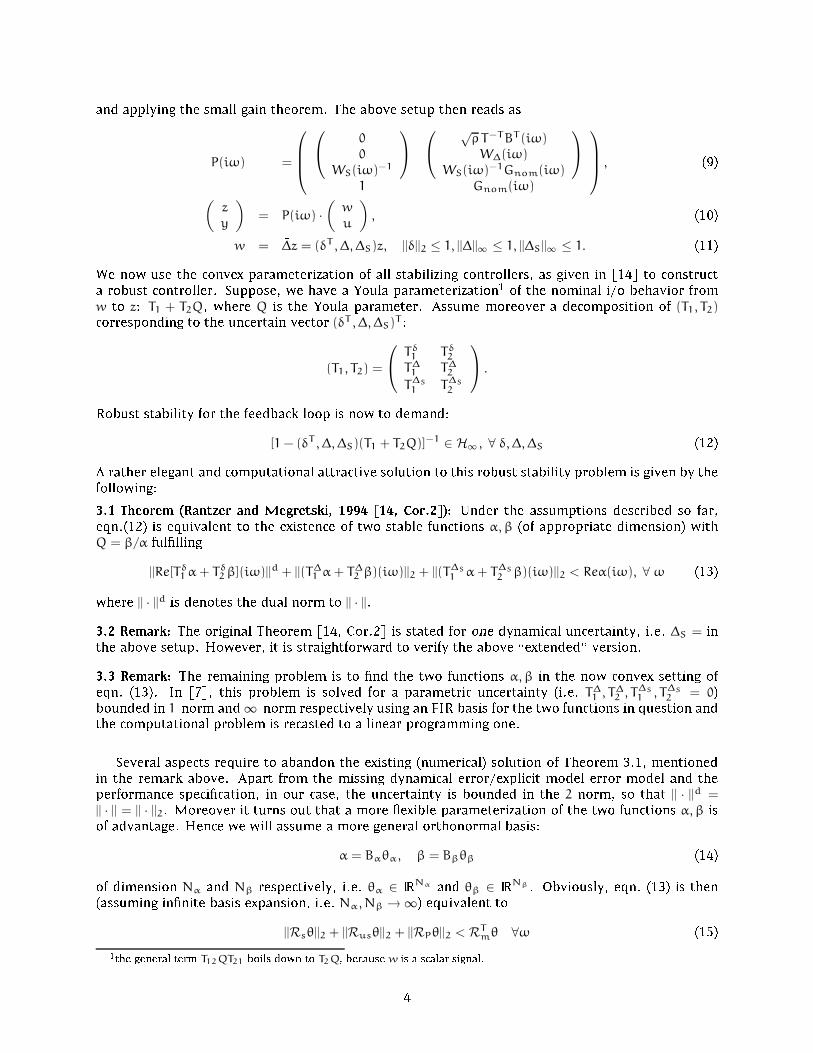
Figure 2: Nominal model (solid) along with the uncertainty region arising from parametric uncertainty

(shaded) and the real plant (dashed).

the gap between lhs and rhs achieves its maximum, when a ↘ −1, which hints to the fact that the

choice of a Laguerre pole for α(z) makes the inequality for robust stability for rank one uncertainties

(13) less restrictive.

3.5 Remarks

• If the problem is infeasible (i.e. the set of controller, ful�lling (29-34) is empty), we still can

analyze this by increasing the two types of uncertainty or relaxing the bounds on the sensitivity

function.

• Some approximation has to be applied to solve the problem computationally: limiting Nα, Nβ(the orders of the two functions α,β) to �nite values is most welcome from the control design

point of view, because this limits the order of the controller (which is calculated back viaQ = β/α

and a lower linear fractional transformation) to a reasonable size. Calculation of low order sub-

optimal controllers from the Youla parameterization of parametric uncertainties has been treated

in [1].

• The problem, that the frequencies have to be discretized somehow can be attacked using a dual

formulation of the problem [7]. Wewill address this problemby an appropriate search algorithm

in combination with iterative frequency gridding.

• The check for robust stability under parametric uncertainties does, however, not require a fre-

quency gridding but is solvable via a single LMI using state space realizations, see [13].

4 Example

Identi�cation: We use the same experimental environment as reported in [5]. 4000 data points are

collected and a second order nominal model, based on a Laguerre expansion (with pole located at

z = 0.96 is identi�ed, assuming an UBB noise of size δn = 4.9. This leads to the nominal model

Gnom(z) = 0.016 z−0.76(z−0.96)2

. The parametric uncertainty in terms of uncertain coeÆcients in the Laguerre

expansion is given by a 2-dimensional ellipsoid of volume 0.0614 and its image in the frequency domain

is depicted in Fig. 2.

7

10−2

10−1

100

101

102

10−4

10−2

100

102

Mag

nitu

de

Nominal plant (b−) and Real plant (r−−)

10−2

10−1

100

101

102

10−4

10−2

100

102

Frequency

Mag

nitu

de

Nominal error (b−) with uncertainty region

Figure 3: Upper plot: Nominal model (solid) along with the unfalsi�ed uncertainty region arising from

the model error model (shaded) and the real plant (dashed). Lower plot: Nominal error model (solid)

along with its uncertainty region (shaded), which includes zero for all frequencies.

In order to cope with the dynamics, not caught in the set of second order (stable) models above,

we identify a model error model. For simplicity, we parameterize the set of model error models via

a Laguerre basis of order 25. Following the strategy described in [5], a pole location of z = 0.95

produces a minimal, non-falsifying error bound of δe = 1.3. The result is reported in Fig. 3. In order

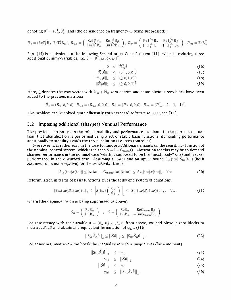
to calculate the generalized plant in eqn. (9), we need to describe the maximum amplitude of the

model error model by a weighting function W∆. As the complexity of this weighting function will

a�ect the complexity of the controller, we pick a rather rough (and low order) description, which is

depicted in Fig. 4.

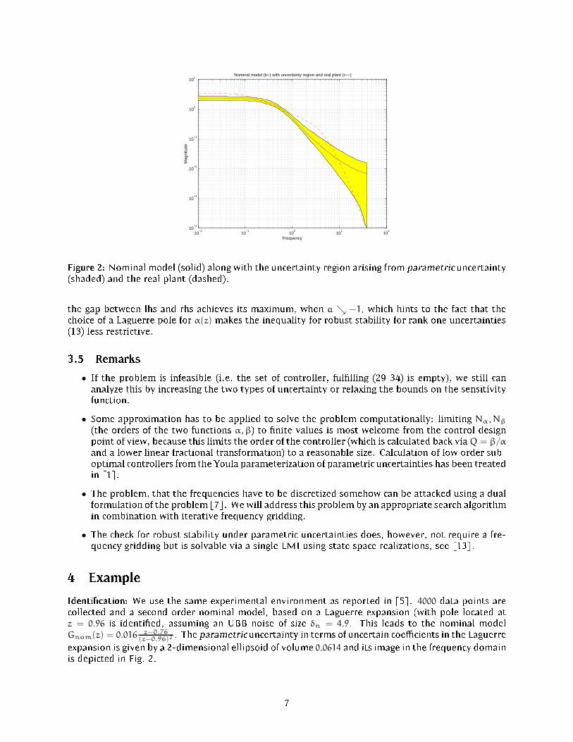
Performance speci�cations: We will compare two di�erent upper bounds for the nominal sensitivity

function (where S2hi can be seen as a \relaxed" version of S1hi, as visible in Fig. 5). The lower bound

for the nominal sensitivity function is visible for instance in Fig. 6. The upper bound WS on the

robust sensitivity function is basically a forbidden area at low frequencies and is depicted in Fig. 5

(dash-dotted) as well.

Controller design: Design 1: We prescribe the (sharper) upper bound for the nominal sensitivity

function S1hi, but no upper bound for robust sensitivity (in order to illustrate the interplay between

performane speci�cations and choice of basis functions for α and β). We have to increase the length

of the basis expansion to about Nα = 12 and Nβ = 6 to obtain a nonempty feasible set. The pole of

α is chosen to pα = −0.9 (according to the recommendation given in Subsec. 3.4 above) and pβ = 0.9

respectively. The result of the controller design is reported in Fig. 6. We did not pose any restriction

on the disturbed sensitivity function, nevertheless, we can check the obtained result a-posteriori

according to [3]. To transfer these results to our setup is straightforward and for completeness stated

in Propositions A.1-3 (see App. A). The answer is that neither upper nor lower bound hold in the

case of parametric uncertainty, whereas no statement is possible for the dynamical uncertainty (the

suÆcient condition does not hold). This may be expected immediately by looking at Fig. 6 (lower

plot). We note that we cannot conclude that there is therefore no solution to the robust sensitivity

problem, as we pick any solution form the feasible set of controllers. This underlines the importance

of incorpocating robust performance demands directly from the beginning in the design procedure,

and not a-posteriori.

Design 2: We relax the performance demands and use S2hi as upper bound for nominal sensitivity;

as in the �rst design, no robust sensitivity is demanded. Now the problem is solvable with a less

complex controller, in particular, we choose lower orders Nα = 7 and Nβ = 2 but the same poles as

8

10−2

10−1

100

101

102

10−1

100

101

Frequency

Mag

nitu

de

Maximum dynamical uncertainty (b−) and Amplitude of weight W∆ (r−−)

Figure 4: Approximation of the maximum dynamical uncertainty (solid) by the amplitude of a 9th

order weight W∆ (dashed).

10−4

10−3

10−2

10−1

100

101

102

10−3

10−2

10−1

100

101

Frequency

Mag

nitu

de

Shi1 (b−), S

hi2 (r−−),W

S (m−.)

Figure 5: Two di�erent upper bounds for the nominal sensitivity: S1hi (solid) and S2hi (dashed). The

upper boundWS for robust performance is a weaker restriction (dash-dotted).

9

10−2

10−1

100

101

102

0

2

4

6

8

10x 10

24

robu

st s

tabi

lity

crite

rion

Criterion evaluated at SOCP freq’s (k−) and SOCP freq’s (kx)

10−3

10−2

10−1

100

101

102

10−6

10−4

10−2

100

102

Frequency

Sen

sitiv

ity 1

−G

Q

Figure 6: Robust controller design with S1hi as upper bound for nominal sensitivity; no upper bound

on robust sensitivity is posed. Upper plot: Criterion function for robust stability (rhs of eqn. (29)),

evaluated at a set of test frequencies (crosses). Lower plot: nominal sensitivity function (solid) and

desired upper and lower (nominal) bounds (dashed).

above: pα = −0.9 and pβ = 0.9 respectively. The result of the controller design is reported in Fig. 7.

The result of the a-posteriori check for robust sensitivity is that neither upper nor lower bound hold

in the case of parametric uncertainty, whereas the upper bound does hold for dynamical uncertainty.

An additional experiment shows, that the feasible set remains non-empty, when choosing the

pole pα in the range [−0.9,−0.6], but becomes empty when moving it towards pα = −0.5 (checking

a reasonable amount of poles pβ for a constant order of both bases), which supports the remark on

pole choice for Bα close to −1 given above in Subsec. 3.4.

Design 3: The nominal speci�cations are the same as in the second design. Additionally, we de-

mand robust performance i.e. the sensitivity function has to obey ||W−1S ·S(δT , ∆)||∞ ≤ 1 for admissible

parameters, WS is depicted in Fig. 5 (dash-dotted). This problem can be solved by a more complex

controller, for instance choosing Nα = Nβ = 10 and the same poles as above: pα = −0.9 and pβ = 0.9.

The result of the controller design is reported in Fig. 8.

5 Conclusions and Future Works

We presented a straightforward framework for identi�cation oriented robust controller design. The

model set, directly identi�ed from data, is based on our previous works on model error modeling

and model validation techniques. The set of all robustly stabilizing controllers, that additionally

guarantee nominal performance, is characterized by a system of second order cones, which can be

eÆciently solved using interior point algorithms, well known from convex programming.

The interplay between the di�erent aspects (stability, performance) of the controller design can be

analyzed in this framework. Moreover, the interactions between identi�cation and controller design

can be analyzed as well: especially one can investigate the in uence of the identi�ed model on the

controller design. If, for instance, the design of a robust controller is impossible for a certain model

set, is it possible when using another basis for the model set (thus, we change or improve the model

set without collecting new data)?

These two aspects will be studied more closely in future works. Another topic of future research

is to explore, which other forms of parametric uncertainties will �t into this framework in order to

cope better with uncertain physical parameters for instance.

10

10−3

10−2

10−1

100

101

102

0

2

4

6

8

10

12x 10

25

robu

st s

tabi

lity

crite

rion

Criterion evaluated at SOCP freq’s (k−) at SOCP freq’s (kx)

10−3

10−2

10−1

100

101

102

10−6

10−4

10−2

100

102

Frequency

Sen

sitiv

ity 1

−G

Q

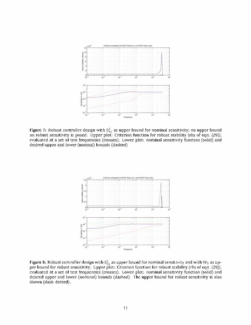
Figure 7: Robust controller design with S2hi as upper bound for nominal sensitivity; no upper bound

on robust sensitivity is posed. Upper plot: Criterion function for robust stability (rhs of eqn. (29)),

evaluated at a set of test frequencies (crosses). Lower plot: nominal sensitivity function (solid) and

desired upper and lower (nomnal) bounds (dashed)

10−3

10−2

10−1

100

101

102

0

0.5

1

1.5

2

2.5x 10

24

robu

st s

tabi

lity

crite

rion

Criterion evaluated at SOCP freq’s (k−) and SOCP freq’s (kx)

10−3

10−2

10−1

100

101

102

10−6

10−4

10−2

100

102

Frequency

Sen

sitiv

ity 1

−G

Q

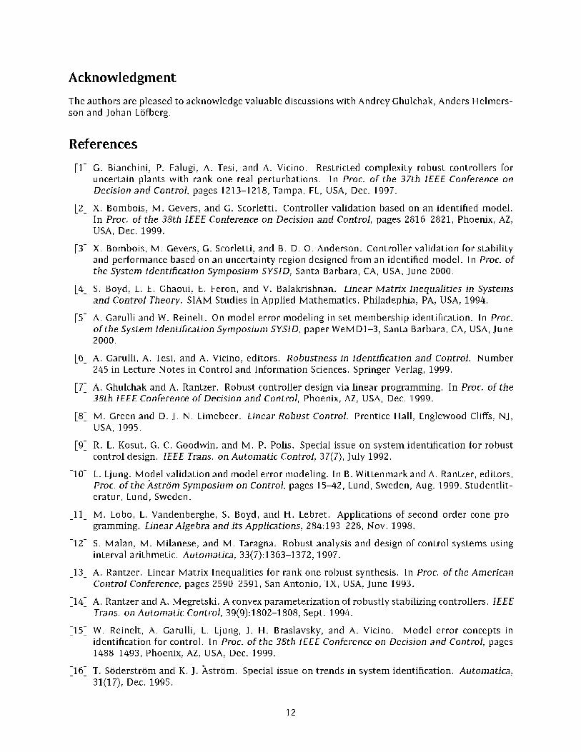
Figure 8: Robust controller design with S2hi as upper bound for nominal sensitivity and withWS as up-

per bound for robust sensitivity. Upper plot: Criterion function for robust stability (rhs of eqn. (29)),

evaluated at a set of test frequencies (crosses). Lower plot: nominal sensitivity function (solid) and

desired upper and lower (nominal) bounds (dashed). The upper bound for robust sensitivity is also

shown (dash-dotted).

11

Acknowledgment

The authors are pleased to acknowledge valuable discussions with Andrey Ghulchak, Anders Helmers-

son and Johan L�ofberg.

References

[1] G. Bianchini, P. Falugi, A. Tesi, and A. Vicino. Restricted complexity robust controllers for

uncertain plants with rank one real perturbations. In Proc. of the 37th IEEE Conference on

Decision and Control, pages 1213{1218, Tampa, FL, USA, Dec. 1997.

[2] X. Bombois, M. Gevers, and G. Scorletti. Controller validation based on an identi�ed model.

In Proc. of the 38th IEEE Conference on Decision and Control, pages 2816{2821, Phoenix, AZ,

USA, Dec. 1999.

[3] X. Bombois, M. Gevers, G. Scorletti, and B. D. O. Anderson. Controller validation for stability

and performance based on an uncertainty region designed from an identi�ed model. In Proc. of

the System Identi�cation Symposium SYSID, Santa Barbara, CA, USA, June 2000.

[4] S. Boyd, L. E. Ghaoui, E. Feron, and V. Balakrishnan. Linear Matrix Inequalities in Systems

and Control Theory. SIAM Studies in Applied Mathematics, Philadephia, PA, USA, 1994.

[5] A. Garulli and W. Reinelt. On model error modeling in set membership identi�cation. In Proc.

of the System Identi�cation Symposium SYSID, paper WeMD1{3, Santa Barbara, CA, USA, June

2000.

[6] A. Garulli, A. Tesi, and A. Vicino, editors. Robustness in Identi�cation and Control. Number

245 in Lecture Notes in Control and Information Sciences. Springer-Verlag, 1999.

[7] A. Ghulchak and A. Rantzer. Robust controller design via linear programming. In Proc. of the

38th IEEE Conference of Decision and Control, Phoenix, AZ, USA, Dec. 1999.

[8] M. Green and D. J. N. Limebeer. Linear Robust Control. Prentice Hall, Englewood Cli�s, NJ,

USA, 1995.

[9] R. L. Kosut, G. C. Goodwin, and M. P. Polis. Special issue on system identi�cation for robust

control design. IEEE Trans. on Automatic Control, 37(7), July 1992.

[10] L. Ljung. Model validation andmodel errormodeling. In B. Wittenmark and A. Rantzer, editors,

Proc. of the �Astr �om Symposium on Control, pages 15{42, Lund, Sweden, Aug. 1999. Studentlit-

eratur, Lund, Sweden.

[11] M. Lobo, L. Vandenberghe, S. Boyd, and H. Lebret. Applications of second-order cone pro-

gramming. Linear Algebra and its Applications, 284:193{228, Nov. 1998.

[12] S. Malan, M. Milanese, and M. Taragna. Robust analysis and design of control systems using

interval arithmetic. Automatica, 33(7):1363{1372, 1997.

[13] A. Rantzer. Linear Matrix Inequalities for rank one robust synthesis. In Proc. of the American

Control Conference, pages 2590{2591, San Antonio, TX, USA, June 1993.

[14] A. Rantzer and A. Megretski. A convex parameterization of robustly stabilizing controllers. IEEE

Trans. on Automatic Control, 39(9):1802{1808, Sept. 1994.

[15] W. Reinelt, A. Garulli, L. Ljung, J. H. Braslavsky, and A. Vicino. Model error concepts in

identi�cation for control. In Proc. of the 38th IEEE Conference on Decision and Control, pages

1488{1493, Phoenix, AZ, USA, Dec. 1999.

[16] T. S �oderstr �om and K. J. �Astr �om. Special issue on trends in system identi�cation. Automatica,

31(17), Dec. 1995.

12

A A-posteriori robustness check of the bounds on nominal sensitivity

Once the controller is established, an a-posteriori check whether the imposed bounds on the nominal

sensitivity function hold or not in the case of full uncertainty as given in eqn. (8) is possible. Using

notation introduced in the beginning of Subsec. 3.1, we are in need to check the following inequality

for all frequencies ω and for all admissible perturbations, i.e. ||δ||2 ≤ 1, ||∆||2 ≤ 1, which we call the

\robust sensitivity problem":

Slo(iω) ≤ ||1−Q(iω)Gnom(iω) −√ρQ(iω)B(iω)T−1(iω)δ−Q(iω)W∆(iω)∆(iω)||2 ≤ |Shi(iω)| (35)

This gives a couple of obvious possibilities to check the sensitivity in the case of uncertainty (where

the �rst one is somewhat related to the discussion in [3]):

A.1 Proposition: Robust sensitivity in the face of parametric uncertainty, i.e. ∆ = 0 in eqn. (35) is

equivalent to the following LMIs feasibility problem:

∃τlo > 0 : τloΓ ≥ Γlo(iω), ∀ω (36)

∃τhi > 0 : τhiΓ ≥ −Γhi(iω), ∀ω, (37)

where the �rst one accounts for the upper bound on the sensitivity function and the second one for

the lower bound, using the following abbreviations:

Γlo(iω) =

(α2(iω) α21(iω)

α21(iω)T |Γ1(iω)|2 − |Shi(iω)|2

), Γhi(iω) =

(α2(iω) α21(iω)

α21(iω)T |Γ1(iω)|2 − |Slo(iω)|2

)Γ =

(Inom 0

0 −1

), Γ1(iω) = −Q(iω)Gnom(iω), Γ2(iω) = −Q(iω)B(iω)

√ρT−1(iω),

α2(iω) = ReΓ2(iω)TReΓ2(iω) + ImΓ2(iω)

T ImΓ2(iω)

α21(iω) = ReΓ2(iω)TReΓ1(iω) + ImΓ2(iω)T ImΓ1(iω)

and Inom is the identity matrix of the same dimension as the order of the nominal model Gnom.

Proof: Let ∆ = 0 in eqn. (35) and apply S-procedure, see [4, sec.2.6.3]. 2

A.2 Proposition: A suÆcient condition for robust sensitivity of the upper bound Shi in the face of

parametric and dynamical uncertainty, is that the following inequality holds for all admissible per-

turbations, i.e. ||δ||2 ≤ 1, ||∆||2 ≤ 1:

||1−Q(iω)Gnom(iω) −√ρQ(iω)B(iω)T−1δ||2 + ||Q(iω)W∆(iω)||2 ≤ Shi(iω) (38)

Proof: Triangle inequality and ||∆||2 ≤ 1 in eqn. (35). 2

A.3 Remark: Suppose, the test of the suÆcient condition above fails, letting δ = 0 in eqn. (38) yields

a suÆcient condition for the case of dynamical uncertainty only.

13