General Disclaimer

One or more of the Following Statements may affect this Document

This document has been reproduced from the best copy furnished by the

organizational source. It is being released in the interest of making available as

much information as possible.

This document may contain data, which exceeds the sheet parameters. It was

furnished in this condition by the organizational source and is the best copy

available.

This document may contain tone-on-tone or color graphs, charts and/or pictures,

which have been reproduced in black and white.

This document is paginated as submitted by the original source.

Portions of this document are not fully legible due to the historical nature of some

of the material. However, it is the best reproduction available from the original

submission.

Produced by the NASA Center for Aerospace Information (CASI)

https://ntrs.nasa.gov/search.jsp?R=19840008556 2018-06-05T01:52:07+00:00Z

Semi-Annual Progress Rpeort4

March 31,• 1983MVI ;

R.

^ Tr ) - w to -

j (E84- 10077) OCEDNOGRAPHIC AND P54-^16624MET.EOROLOGIC4 L RESEARCH BASED ON THE DATAPRODUCTS OF 5EASAT - Semiannual Progress

eport (City Coll..of the City Univ. of New Cnclas1 .)ck. f 57 h HC A 04111E A01 CSCI 05B G3/43 00077

"Oceanographic and Meteorlogical ResearchBased on the Data Products of SEASAT"

1

0

Grant No. NAGW-266

Professor Willard J. PiersonPrincipal Investigator

Institute of Marine and Atmospheric Sciences

The City Collegeof

The City University of New YorkConvent Avenue at 138th Street

New York, N.Y. 10031

F

N

1

l

^ 1

r

DRAFTPRELIMINARY

LIMITED DISTRIBUTION

SYNOPTIC SCALE WIND FIELD PROPEil`141ES

FROM THE SEASAT SASS

<. s

t

{ By

r

Willard J. Pierson, Jr.r Winfield B. Sylvester

Robert B. Sal£i

CONY Institute of Marine and Atmospheric Sciences al;The City College

The City College of the City University of New York

Convent Ave. at 138th St.New York, NY 10032

Prepared forThe National Aeronautics and Space AdministrationWashington, ,DCContract NAGW-266.

,

6{i {

ABSTRACT

N

Dealiased SEASAT SASS vector winds obtained during the GQASEX program

have been processed to obtain superobservations centered on a one degree by

one degree grid. The results provide values for the combined effects of

mesoscale variability and communication noise on the individual SASS 'winds.

Each grid point of the synoptic field provides the mean synoptic east-west

and north-south wind components plus estimates of the standard deviations of

these mean. These suporobservations winds are then processed further to

obtain synoptic scale vector winds stress fields, the horizontal divergence

of the wind, the curl of the 'wind stress and the vertical velocity at 200 m

above the sea surface, each with appropriate standard deviations for each

grid point value. The resulting fields appear to be consistant over large

( distances and to agree with, for example, geostationary cloud images

obtained concurrently. Their quality is far superior to that of analyses

based on conventional data.

^^ A A

sz

•4 ,^

!+

Qu

ii ! {

INTRODUCTION

c

The ability to determine the winds in the planetary boundary layer

over the oceans of the Garth by a radar scatterometer called the SASS on

SEASAT has been demonstrated. The objectives of the SASS program, were met,

and perhaps exceeded, as described by Lame and Born (1982). A problem was

identified, when it was recognized that errors in the conventional data need

to be better understood. The sources for the differences between a SASS-1

winds, a conventionally measured,wi.nd, and a wind derived from a planetary

boundary layer analysis using conventional data are many and varied. Yet to

be produced are planetary boundary layer analyses of the wands based on the

SEASAT SASS-1 data only, augmented by a minimum amount of conventional data

such as atmospheric pressures at the sea surface and air sea temperature

differences ; The purpose of this investigation is to prepare and analyse

wind fields from the SASS data.

The three most important applications of SEASAT-SASS-like data in the

future will be (1) the correct description of Che winds over the entire global

ocean at an appropriate resolution, (2) the use of these data to produce

vastly improved initial value updates for computer based synoptic scale

numerical weather predictions and (3) as shown, by O'Brien, et al. (1982),

the .specification of the wind stress field and the curl of the wind stress at

the sea surface for oceanographic applications. In this investigation, synoptic

scale vector wind fields with a known error structure will be produced at a

one degree resolution from the SEASAT SASS-1 GOASEX data. These synoptic

scale wind fields will be used to compute fields for the horizontal divergenceA

of the winds in the planetary boundary, the vertical velocity at 200 meters,

and to determine the error structure of the resulting fields. The vector wind w.,

stress fields can then be found from the vector wind fields, and the errors in

these fields can be computed. Finally, the curl of 'the wind stress can be *;,

computed,,with a specified error structure.

S ^. p

Certain assumptions need to be made concerning the accuracy of the present

SASS-1 model function and the wind recovery algorithm. Also the drag^ A r

coefficient that relates wind stress to the wind at ten meters is a matter of

some uncertainty. If'any of these assumptions need modification and updating' 3

i

In 5

ii

t x

t

,t for future systems, the main results of this study will still be applicable.

i As a•first effort, the atmosphere will be assumed to be neutrally

stratified. An application of the Monin-Obukhov theory for non-neutral

stabilitj as in Large and Pond (1981) would provide an improved wind

field at 19.5 (or 10) meters for the computation of divergence. The field 1

for the air-sea.temperatuxe difference would be needed to an accuracy

"•? comparable to the neutral stability wind field.

R1

i

f

s

Ir

3

t .^1r

DATA

The data used in this inveutigation were provided by the NASA Langley

Research Center. They consist of the de-aliased SASS-1 vector winds produced

as the final product of the analysis of the SASS data for the SSASAT orbit

segments chosen foixIntensive study during the Gulf of Alaska SSASAT

Experiment (GOASEX). Preliminary resultss for this experiment are described

by Jones, et al. (1979). Two workshop reports, Born, et a1. (1979) and

garrick, et a1..(1979), plus a'summary of conventional data analyses, Woiceshyn

(1979) give additional details..

The SASS-1 model function was based on the JASIN data with results

summarized by Jones, et al. (1982) , Schroeder, et al. (1982) Moore, et al.

(1982) and Brown, et al. (1982). As described by Jones, et al. (1982), the

GOASEX data were reprecessed , 'by means of the SASS-1 model function. De-aliasing

was accomplished by selecting that wind direction closest to the planetary

boundary layer wind fields obtained from conventional data. The model function

recovers the effective neutral stabilit; , wind at 19.5 meters.

The wands recovered from the SASS . are very densely concentrated over the

swath scanned by that instrument on SSASAT. Examples can be found for the raw

data density in Wurtele, et al. (1982). Only pairs of backscatter measurements

90 0 apart were used to obtain winds with all combinations of vertically (V)

and horizontally (H) polarized measurements (i. e. V with V, H with H, V with

H and H with V). For this study, no distinction has been made for possible

effect of polarization. The communication noise errors could be quite

different for the different polarization combinations.

A sample of z, data listing for a particular GOASEX pass is shown in

'Table 1a and lb. The data for a north bound pass of revolution 1141 are

shown. The central part of the full table is repeated in both la and lb.

In order, the values tabulated in the twenty one columns (as numbered

with 11, 12 and 13 repeated) are as follows:

(1) Revolution Number,(2) the'latitude of the mid of the line connecting the centersers

of the two cells used in the calculation,(3) the longitude as above,

L.

I

i>>

E)

f

A pr ^

^1 F

l''Ai^•^

t ^` sIy4 1

jtf}

^

L

^^ 1

^ r

,1

4

(4) the wind speed in meters; per second from a boundary layer model,(5) the neutral stability wind speed from the SASS,(6) the from which wind direction in degree from a boundary layer

model clockwise from north,(7) the closest alias wind direction from the SASS,"(8), a quality code for the accuracy of the boundary layer wand,(9) a code for the estimate of the precipitation in the area,(10) the distance between the two SASS cells,(11) the average pf the values in the next two columns,(12) the incidence angle in degrees of the forward beam,(13) the incidence angle of the aft beam,(14) the pointing direction of the forward beam in degrees clockwise

from north,(15) the pointing direction of the aft beam,(16) the backscatter in decibels measured by the forward beam,

(17) the backscatter for the aft beam,(18) the noise standard deviation for the forward beam in per cent

(multiply the antilog of the backscatter by this number dividedby 100 to get the standard deviation of the measurement),

(19) the NSD for the aft beam,(20) the polarization o,f the forward .beam (0 = H, 1= V) and(21) the polarization of the aft beam.

in this a?LVesti g ati on, , onlyy the! elements of the data vector corresponding

to LAT, LONG, WSP, WDR and FOR AZ were used to derive tho reslxlts. For some

portions of some of the SASS swaths, the boundary layer conventional winds

differed substantially from the SASS winds. The data base for the conventional.

fields will be discussed later. Future scatterometer systems may eliminate.

the need to remove aliases as in Pierson and Salfi (1982), for example. Wind

fields produced by the methods described herein would then be independent of

conventional data sources, ex:ept sea surface atmospheric pressure and`., perhaps,

air temperatures. Sea temperature is remotely sensed and does not vary

.rapidly.

The GOASEX data set provided by NASA Langley contained the results of the

analysis of nine passes over the North Pacific. These were portions of

revolutions 825, 826, 1141, 1183, 1212, 1226, 1227, 1298 and 1299. Extensive

depictions of conventional data are available for those five orbit segments

underlined above (Woiceshyn (1979)). , a

i

Q!Yr

t r

{

E

j,

`s

11

qt'

E

4

C

t

ORIGINAL PAGE 19OF POOR QUALITY

atonooc000cga4^c:aaouc^c^ocooraac^r^ar.^oaor,^ar^nosaM f- NO% rr* Nhh lnP- r--N- tnw tn NhnulN knP-N P0N00 0M 00N0M

ri tt- W tt • 4 • • r • r • r • • • • • Y r • • • • • • • • 0 • 1 • • r • • o • •rtT rr WW oDrlr4r-1r4 h r hhP rtr r4C7PN0NN r rN 4 *

hy M M m Mcg*.r .t%rrkr r a* r'r-rr %rr r r -r - r r ul 4nr ul toln ulu1 tnusu% in

40004 OOCCClOCi Q0004004:.0AOOO4a4a p GOOC ^4^Ot74:1C;-N cY 4- rr-O M m r-4 m cONPP N Cf P Hr-4 %r r4r-4'r-4 ,t r-+ MM m O MMd m -o O r-r` CIO

LA. r r r' ^ •r P oa m P opw, P O O m m m M f+ M Mmf`-hr-- h h r~ h h'G r-4O0 r4H. (-Mm m M mmM 4rl m m M mM M rrr r r .r rr r r r r r•t^.tulul ►nM1' u^u1

-aa4:^oacvac^acaot^ oco^a^^aca000aoaa+p c oraor^oKaiar:^o,^ 4- .G to ^ r m -r m N r m N it° m N O- 45a m P m ao M m tr1 t11 -0 1t1 ut ^c'i t1 .o u1 111 m ur u1 (^

.J LU • • • • • • • • • • r • • 1 • • • • • • • • • • • • r • • 1 • • • • • •%r %t c -00 00 0 00 00C mMLCI0ulMtntnaoaoPcpcOPaaCY*HNNHNN

rr4 F- m rri mmen rw .rr r•r rr'r r r r •t rr r-r.t r r r rr .r r W'r LC) H 0 U*) ulJ F-000 0 QOO DO 0 a 0 0 0 0 Q 0 C3 0 0 0 a 0 0 ci 0 CAo .d©J00

4„t p J 11 4/1 • • • i a ^, r • • p • • • • • • • • • • • • • • • • • r • • • • • 00 • • •C) r-► W W t--r r N r-4 q M 111 h CO h -O O+ -o t0 Cl to r-- O ^o r- Cl P F h cc r- 0 , co t• r-4 O N r- Z to r- M

r-a t.1 1/f 0 N m N N N r-4 0-4 r-► .-4 r-4 r4 r-4 N r1 ra , N N r-1 N r-4 H N r'r r-4 N r4 M cV 0-4 N Nft CL

r" 4 f„r

01 Wr .r rr r r=t r 'M M MM.m m mmr r-r -r^t rr M M MMMMMMMMMMMr-4w

tia

U .JQ r4 H r-4 r-4 r-1 r) r4 r4 r4 r-4 H r1 H r-4 r-4 r 1 e-4 H r4 r-4 r4 H r-1 r-4 r4 H r4 r-4 H r4 r-1 H r-4 ri r-4 r4

E~ 00 OO d

44 NN-OP W NMN•V0 NM -OWMM PNW04T r4 r-4 u1N0 Q tx. NtnMH0 tnPp' • • • • • • • • • • • • • • • • • • • • • Y • U • • • • • • • • • •

^ O a r 4 P w 4 PP r -OaoC^ P Clo ol;y r m h u+ P M tn h• mrn r

.• c; C4 z t M"- .z

:m 'o -D U) wO vim -O ^nr-Z-Om cn Pr--u1 rr-hd -Or--%,o- ^om M m-0 r m%O ,-t'

N N N N N N N N H N 11E N N N N N N N N N N N N N N N N N N N N N N N N N Nw to r- m 111 m 0% r-/ In r`- O` ^c w O cT r-4 O- co m O O N U1 in P C1 1 -r -1 00

C 10 DWMMPP C''wM0P ,o-O .0hf--M%Dr- rLn tnZ to 'or NNM M N M's, NPPO O PW 4 r- h r- N h h r-- r+- 4-- ^ r-- r- t-- r- r- r- 1` h h h 1- h-- ti ti h h P h Nr- r~ 10 -o h r--O N N N N N N N N N N N N N N N N N N N N N N N N N N N N N N N1N N N N N0 a.c]an 0= 0x 0Z.O4-r-rr4r4-t WIn hM m to o r-4 r%r .O N- 4; NM f- toP- NOS

:x

P t9' NCt ON PQN P CJ 41-1 MOb ON r4r-lr-i .-40O` riQ p r4taP tJP QhHCQr4r-4 N H N N r4 NN 1-4NNNNN N NN NNNA4Nr-fN NNNNr-4NHf%JH

m n.nLA0 rtnulr0 0P P Cpl PwmNmNH0%cTmrrm4rrrV(O C.1rrItrr//f • • • r o • • s • • a 4 • • • r • q • • • • • • • • • • • r • • r. • •, •3 r-1 r^4 --1 rd r♦ N r-1 r-4 N N N 1-4 14 ri r-4 r-4 N N N N N •-1 r^1 N of N N N N -4 N N N N N NQ N N N N N N N N N N N NNNNNNN N N N N N N N N N NN NNN NN N N

W hO' N •t to min'o r-P4-tin-OQOUlri'oOoMr-4Mrw 0 . u1t11-or. o.tu1a lhZNr4Nr-4 r1P'MP--Oto r Nr-1H 0 r`- 0 N r r-4N r4 0-LnM.r N.t 0 -4 r-r^- O r -r LA

C3 • • • w • • • • • • • p • • • • • • • • • • • • • • rr • • • • ♦ • • •E~ Jh hh r--4^P-hti

•Otl^ aO uJaJOCD wP PPPPTP G o O O C tG7OOr4r-Ic^Ir-1.-4

O O A d O rJ O J o to D O J O to O o G A O D O 0 r-4 r-4 r-1 r-1 r-1r r4 r-4 r-4 N ri r-4 r-4 r-4N 114 N N N N N N N N N N N N N N N N N N N N N N N N N N N N.N N N N N NJ r r~ 0 tc1N6'1PNtnPri r PP r oO+(> M r4O N h-O -rr--r- nca H't Q101-rr

4--4 r4 LA1 0 -0M 000 O O/J -t -fir t 0r-- NNMM.0co Co0 r-4N.r In -O PP JQ O t CV Q • • • • • • • • • • • • r • • a • • • • 4 • • a • • • • 4 • • • • • •Jlt M m m mmM m)m mm Mm ,llmm m m mm ^nm m cn MMm,m M ,cr1 MMrnM m m

to Ln u1 to wt to LLl 41 ul to in to to ul Qn ;1 to to ICto , ul 1 to , to in to to to It. ^1 ,n to u1 ul to to in 111

+ r4 r4 r4"4 r-i r4 r-4 rl .r°-4 r'4 r-'t r-4 r'4 r+ r4 r-4 r♦ -4 r4 r4 r4 H r-4 r-4 r♦ -4 r-4 r4 r'4 -'4 r-1 r-4 ^4 r4 r1 r-4r-a WOrrrrrIr r r rr -r.t r .r,t r Ir rr .t r rr rrrrr t r •t rr rIt

w oz r-4 rl r1,r-i r-4 r-4 ri -=4 r4 0-4 r-1 ry r-4 &-j r-4 r4 r-4 r4 r-I r4 r4 r-4 r-4 r4 --1 --4 r-4 r) r-4 rfi r-f ri r-4 ri r4 Hr-4 r4 r4 r4 r4 r-4' r4 rr r-1 r4 r-4 r4 t-4 r4 H r4 r4 ►4 r4 r4 r4 r-4 r-1 r'4 t-4 r 4 r-4 -4 1 r-4 ►4 r-4 r4 rl . r4 -4 r-i

I

S'f

1

i

k i

i

ljtr .

y 4,

.x

rx

i7

a)b.rl

1]0.Hx

r-1

r-4

w

a'w

t . q0t-i

k

w

I

t

r

ORIGINAL PAGE ISOF POOR QUALITY

a ,

41

0 u~. H O rg r-1 OH6.4 0 H:H,01 94H0 r4 0or4Ho a H o o a Hoto H Qr-I0 o4 Q

..J OCQ p O O ri Q O r1 O O r-# 1-j 4a rl O O.O 43 ,H 4^ Q O r-1 C9 •-1 r^ r-1 o r-f rl ^t r-1 O rl 4s. U.

p. ^... • a • • • • • • ' • • • • • • • • • • • a • • • + • • • • • • • • 6NLL/nto r %r r M MMMMM 4"MMMM -r mm mM M ul -rQ%r in^o r Q0aowz<

s ue, ^^u,^PCa o P Oa tT 4b mm,ocrP Pf`- coy-+r1.-^h r~^^^ ri •nr`h-co ti9C^v0^lJ -O^O-O r 44lu1 r ulul^rufl >nfA M m 1T1 MM m M mm M n1M(^! 471M mrP-4 z U.

-O .^ N N an (^ h m •t ^ R-. f'- f~ r ao r h .-1 In ^ IC1 H oD rl (`^ r -4r .-^ H ,r 4n P P^n I- -or MM--4NN aDIn ulHIt r a-mPO fl- Hw m001 M h r r

'-1 Ck 4 CO ay C> P t7- .-4 C7+' P N P P ri O N -L1 G N r* M c: Pz { { { { ri { r 1 ( { r-i { H H H rl rl r-I H rf r-f .-/ r-1 r-1 r-1 r-f rl r-1 r-4 H H r-I

I { 1 1#I 17 1 1 1 1 1 I r 1( 1 1 r 1 1 1

w rr N r r Cr %0Z H 0 0 O r• r- Z Z40 MINNN -dNrlr-1N m tr1 0 Nr-1H Oto oC aD m z 00 H r-t H a 0 O m Jr -3r r- f- M ' 4 - V--.' 1- 0 P4 0 rr v N ffl

^p r-; to • • • • • • • • • • • • • • • a • • • • ♦ • • • • • • • • • w •-{CX LL oJ C7 OO r-1 4m;44Mer4MM^! r NU;U--W)N rmm mhr+l m Wm9-t We

z r-1 ►-I I r-4 9-4 r-1 r4 ri rd H H H H rl HI rl H H r-1 r r r-1

1 H ri rl r-f H -1 r-4 H r rl r-1I r r f I r I I r r I r I r I 1 1 1 r I 1 1 ^ r o 1 1.I

r-1I I

^c In Ylyd r` rr 0'tA%0 N1-4 u1 N001NOC>" M0' 4 %0 AJNF- MIfs IS) In f-O 0Nd r O NN r(`• 0D h P r HU)N O M W m r r

L7 I . 1"4• • a • • • + • • g • • • • • • • • • • • s • • • • • • • • • • •H rt 4 P C" O-P PC? OO C?OQ',^0004 4r-1 O r-1 r-1 rir-1NNNN NN r4NNM M

0 0 0 O 0 rl r-1 H H r-i H H r-1 r-f H r-/ r-4 H r-1 H r-4 r-4 r4 H r-/ rl H H r-4 H H r-4H H H .-4 H rl r-4 r4 r4 H H r-4 r-1 r4 H r-4 rl rl r-4 rl H H r4 H H r-I r-1 r-4 r-1 r4 ri r-4 ri

rir-4m In ul In HH+O MM NW CD *4 ' ruD co OD ul .t4 -r r %OMM MO a CTNO. O N r- %0 400 O NNr/hN (7. rr 0 0%oNNN r C)a rr•t' N N co 0rH aJ

,.t O-Q lz W C7 1; 94 C;a 8 7 a* C' PPCb4 81;O4OC,lrl4rl1l14r4 $;9r-1NMLL r-4Hr-4.4 H Hr-4 , Nr4H HrlHNNN NNNNNNNNNNN N N N N N

rr) 4-F- M %0 .4* r Nfl- r- U1hh11 f-r-InwuiN hIn LnNUl hhPOP-[0?OMt^Or l LL. W • • • • • • • • • • • 0 11 • • • • • • • • • • F • • a • • • • • •

st Y r 4 w W, coH HHrl r- + r-1 r4 Hr-1 r r h rrr r hr-PPr4oPN 0 NNr rt--MMMM M r r-s^ y^ r s rr rrr r rr .tr &rin InrinInIn0lnm

•a000c^00000e^eaaeoceaoaac7aaoc^0000e^oocac^' H r r +C* f+n MH a: m N 01 01 N4;91CI H .-f r ri r-4 r4 r r-4m01 m O M m O M 0O P-

00 • • a • • • • • • • • • • o * • • • r • • . • • • • •,.

rr .r .r rP Qa a; V, aDw PCOa;MmMM 4 M M m r- r-h r-P-r—r-- r-0r+OI- MmMMMMM. mMcolMMmM r -r%t.r .trr.r .r4%rr•trrr.tln ►nina000rsoa^crc^oc^c^aac0000^c7aac^a^oaoaoaoo

r-I t~ ^4n ►c,.r mrM N r M N O,oDM P m 40 mm In u1+q Yl z ul ul Mrl W • • • • tr • • • w • r • • ♦ r • • • • • • a • 6 • f. • ♦ • • • •^lzr ZZ Z aC) OQ d QO4 m m 4; 4ul ul ln 4,A W PaDm P ZC;.4NN

t^

itI

b 1..

r

tt

b n^

`s

I

u q1 + y -}^ k

t

3{

An appendix defines the notation

.

THEORETICAL CONSIDERATIONS

The objectives of this analysis of the SASS data are to recover the

synoptic scale wind at a one degree resolution on a spherIcal coordinate4

grid and'to derive synoptic scale Fields for divergence, vertical velocity,

the vector wind stress, and the curl of the }finds stress from these winds.

For use in a synoptic •. scales analysis at sc;^oq initial time, the requirementis for the winds to b,, specified as east-west and north-south components at

integral intersections of latitude and longitude in the form of values as

close as possible to us(Xo'00)

and Vs(A01 0o), where the subscript, s,

designates an error free synoptic scale measurement with synoptic scale

gradibnts accounted for and theix effects removed and with mesoscale fluctua-

tions and instrument errors reduced. The SASS winds were not measured

at the location, X0 , e0 . They contain the effects of mesoscale variability,

and there are errors (sampling variability as an effect of communication

noise and cola; location inaccuracies), in the measurement of the backscatter

that in turn result in errors in the calculated winds.

The locations of the SASS measurements are more or less randomly

distributed in an area around the desired location, X 0 ,00 , but the gradients

in the wand are systematic and need to be considered. If the SASS-1 wind

vector recovery algorithm and model function have no systematic bias, 'the

mesoscale .fluctuations and the effects of communication noise will also be

random and have the same probabilistics and statistical properties within an

area around X0'00.

The individual SASS winds can be combined in such as way that the effects

of ` gradient.s can be greatly reduced as a source of error in finding the wind

at X0 ,00 . Also the random errors introduced by mesoscale variability and

communication noise, can be modeled probabilistically, i,ntew-preted statistically

and greatly reduced by means of the application of small sample theory.

It is not necessary to separate the combined effects of mesoscale varia-

bility and communication noise. Their effects can, however, be considered in

+

.+

t

+

tr .'

t

r

u

wORIGINAL PAGIE 13r OF pOOR QUAL17Yi

€ the interpretation of the results that are obtained. O toa the effects of

communication noise stand out above the effects of mososoale variabilitya

P especially as a function of aspect angle violative to the pointing angles of

1 the radar beams o.£ the SASS.

Consider a number of measurements, all of the same geophysical quantity

h such as some kind of a wind represented by u, made in the s'-me area, that

f` all ought to be nearly equal to the sane value. Those values will. not beequal Por numerous reasons. Conceptually there is some correct (or true)value and the actual values will scatter in a random way about; this correctvalue. The measurements can be described as having a probability densityfunction (pdf) , f (u) , with the usual properties of a pelf, namely,

.. f.W du = 1f

(2)-

and uf(u) du = uf

(3) -00

which is the first moment of the pdf and can be associated with the correct

value.

Moments about u1 as inr

U -u-ul

yield (u - ul) f (u) du= 0 (4)-00

0

and J- (u - ul ) 2 f (u) d u = (h u) 2 (S)

00

Now lot u ul + t:Au (6)

or 't -- (u - zi l AU (7)

so that f,(u) is transformed into f(t) . The pdf•, f(u), is transformed into

,.. f (ul + tAu) Audt _ f* (t) dt (8)t,

M

iff .

___

i

11 t

14'

rt }

t

E

t

i

1

I

i

s.

tN A

V

±a^

gi

a t

S

ji

and f* fit) dt has the properties that ORIGINAL, PAGE 6OF POOR QUALITY

^-00

(t)dte

E

f

OV

_ t f* (t)dt 0 (10)

00 t2 f* (t)dt - 1 (11)

The concept can be generalized if various reasons for the variability

of the measurements can be identified. Suppose that there are, Say, two

causes for the variability that many differ from one set of measurements to

another such that

(Au) 2 = (AU 1 ) 2 + ( Au2 ) 2 (12)

TheYi r}tf^ pelf ran be generalized t o the product •, •••„ ""`^pL ..,v V of two indep endent pdf

f;(t l) • f(t2 ), and (7) becomes

U = u1 + t 1 Aul + t 2 Aug (13)

with obvious extentions, if needed, such as, for example, conditions such

that t and t 2 are not independent and covariances are needed,

Small sample theory can be applied under the assumption that all of

the measurements are for the purpose of learning more about u1 , Suppose

that M measurements are made as in

ui = U + t1i AU 1'.- t 2

Aug (14)

where thb t li and t 2 are from (not necessarily the same) pdf's with properties

defined by (10), (11) and (12), (f* (t) is the convolution of f(t 1 ) and f(t2)) .

The average value of the u is given by (16) from (11)

I

r

I€z.

e

i`

Ti uiM OF POOR QUALITY

,:p ul + M t l i Aul + M t21 Au2t'

f

C2 ul + M ti Au ul + M t ^(A u1 ) 2 + (A U2)2 11 (1S)

and the expected value'of the average is (16).i4

G e, (u)u 1•

(16)

The random variable

1t t l ^Mtli(17)

tl

has a mean of zero and a. second moment of

1}-

M2 rt l) l/M (18)

M r so that as c; represented by

4Zt ul tl (M^ Aul) + t2 (M Au 2)

rul + t * Chi"1 ((Au 1 ) 2 + (Au 2 ) 2 )^ (19)

t

The expected value of u is ul and the expected value of (u-u1) 2 is

lE (u' - u1 )

2 = M-1 ( (Aul) 2 + (Au2 )

21(20)

From a given sample, it is possible to estimate the mean, u, the standard

deviation, Au, and to use the fact that u has a standard deviation with

reference to the desired true value given by M -12 Au where M is the sample

isize.

' 1

1

1

A number of SASS individual wind values can be combined in such a way

as to recover,a single estimate with a greatly'reduced variability. When

these estimates are then combined to form fields, this greatly reduced

F '" variability,,which is known, can be used to find the variability of various

derived fields.

41

I

i Z

f^

f,

Y

e.•OV

kaA

It is well known that the mean of a sample from almost any typical, but

unknown, pdf will be nearly normally distributed by virtue of.the central

limit thebrem so that although the pdf l s of t, ti, and t2 may not be known,

the pdf's of t t and t2 will be close to a unit variance zero mean normal

pdf for most of the values of M that occur in what follnws.

As in any statistical proceedure the moments of a pdf, such as ul,

always remain unknown. The statistics only provide a way to put bounds on

ih6 estimate of u l , that is a,*that are made narrower because of the sample

size. In (15), u, M, (Au )* + (Au (AU) 2 are all known statistics, where.1 2)

(Aul ) 2 + (Au

2 ) 2 is an estimate of the variance from the sample. Thus (15) can

be rewritten asr.

U w u.. t M-" Au (21)

where all is known on the RHS except t (the minus sign is not too relevant):.

The values of u I when found at a grid of points form a field consisting of

values of x plus a quantity that provides information on the variability

of

A#^

W`

As an example, if u is 10.73 m/s, Au is 2 m/s, and M is 25, then abouttwo thirds of the time it would be expected that the interval 10.33 to 11.13m/s would enclose the true value, u 1 . If sampling variability quantitiesare kept track of in the finite difference calculations of properties of thewind field, they provide estimates of the sampling variability of theseproperties.

ORIGINAL PAGL-. 12

OF POOR QUAL

i.

tf

i

^. 4

y a`^

1 '^ s

e,r

PRELIMINARY DATA PROCESSING ORIGINAL PAQ&^: C

OF POOR QUALM

The first data processing step was to sort the data shown as an example

in Tdble.l for each revolution into overlapping two degree by two degree sets

centered on the one degree integer values of latitude and longitude. The

vector winds found front combining many individual SASS winds around a grid

point of a model have been called superobservations. A given SASS wind could

be found in tour different sets. As in Figure 1, a given set of SASS winds

would have latitudes and longitudes that varied from X0 - 1 to X0 + 1 and 0 0 -1

to 00 + 1.

A preliminary investigation suggested that the two solution cases and

the base of the "Y" in three solution cases gave both directions and speeds

that were systematically different from the other directions and speeds

within a given two degree square. Since the original data set gives the

pointing direction of beam 1, say, X 0 , dealiased winds were checked to see

if the directions were within X_ ± 1 0, X_ plus 89 0 to 91 0 , X plus 1790 to

1810 , and X0 plus 269 0 to 2710 . 0 If they were, those particular data vectors

were removed from the set. In Table la, for example, the data corresponding

to SASS directions of 288.8, 289.3, 289.6 and 290.3, were deleted.

When centered on X0 and 00, the latitudes and longitudes can be.trans-

formed by subtracting X 0 and 00 from each element in the set. The locations

of each SASS wind will then be defined by values of, AX and A0 that both

range between plus and minus one.

r .

t

x

i

u

E

jj

9j

i

c ¢r

Y iff f(} m

T

ORIGINAL PACE 19OF POOR QUALITY

J34

po+2

2,

eo+

5 G

ea

7 8 9 10

eo-I

11 12

eo-2Xo--2 Xo I Xo x0+1 A0+2

r-ig. i i-he Z° by Z° Overlapping Spherical CoordinateGrid Centered on Integer Values of Latitude andLongitude.

a ,

i

o

13

w

f

f

r

ORIGINAL PAID7% 6-OF POUR QUALITY

The average latitude and longitude for the data set will be equations

(22) and (23) for the N + n values in the 2 degree square.

1 N+nFlo ,+ AA1 = :0 + N

+n S Aar (22)1 ,

N+ne,o 4. A8I so + N+n A6

(23)1

The values of AA and Y -- will usually be close to, but not exactly, zero.

The location of this point will be in one of the four quadrants of the heavy

square in Figure 1. By selectively removing n of the data vectors in the set

based on the location of ZX and A8, it is possible to reduce both -AX and Ee

for the remaining subset below some preassigned minimum as in equations (24)

and (25)

NXo + AT = ao + N u AX. (24)

IN

eo + De = eo + N pe.

(25)1This subset of data for each two by two degree square was processed

further to obtain the results to follow. Also needed for later use will

be the average values of (AX i)2,

(Ae i ) 2 and (AXi•A®i).

R

r

ii

J

5

i

't

WI?JD VECTORS

S

1

^K }

m

F F

The N value for the winds in each data set consisted of a speed and a

(from which) direction (meteorological convention, clockwise from north).

The directions were averaged to obtain a value for the average direction as

in (26) where the summation notation is abbreviated.

X = N Xi (26)

Each.wind was then resolved into a component in the direction of X

and a component normal to as in (27) and (28),

VPi = jVj i cos (Xi - X) (27)1

j

(iyl

^ a

r4^ t

F

!F

,

I i

i

I

n.

s 't

N t

t ^E t

1

!a

f S

I

I

ORIGINAL PACE C

VNi = J V j i sin Cxi -

OF POOR QUALITY (28)

These components were averaged to obtain (29) and (30).

VP N VPi (29)

VN ` N VNi 0(30)

In all cases VN was essentially zero. The standard deviations of V and

VN about their sample means were also computed as in (31) and (32).

1,Au = 'SD (VP) (I Z (VPi - V

P) ^ ) 12 (31)

Av = SD (VN) (N XVNi VN) 2

) Z

(32)

The processed data at this point consist of the sample size, N, the

mean direction, X, the mean component in the mean direction, V and the

values of AU and AV as located at a point given by ao + 7(with the values

of X0 + Aa and e0 + e located very close to the integer values of latitude

and longitude over the ocean) plus the average values of (AX^) 2 , (Ae^)2

and Aar Aei(i.e. VAR (AX), VAR (Ae) and COV (AXAe).

The "from which" meteorological convention can be converted t a "toward

which" vector by adding 180 0 (mod 360 0). The new direction, clock angle, is

needed for use in analyzing the wind field. The east-west, UX,(abbreviated

as U), and the north-south, V e , (abbreviated as V) components of the three

non-zero I

vectors given by (29), (31), and (32) are next found.

The mean east-west and north-south components are given by (33) and

(34).

U - VP sin + 180 0 ) -Vp sin X (33)e

V V, cos (X + 1800) _ -VP

.cos X (34)

The components of AU and AV from (31) and (32) in the east-west

direction according to the convention shown in Figure,2 are (35) and (36).

' ....:.

m . xr. .,...- ..... :..... .. ., , . ... w .:,,r ...::..4 ... , c«• wm :^.. Ott.,—r „r . ,.— ^....--^..—;_..^._.^.,.^--:...^. _..,..

`14w4ir

ii

,s

e ,

ORIGINAL MUM,,AU = -Au sin X, (35)OF POOR QUALITY

Aug - AV cos X (36)

The components in the north-south direction are given by (37) and (38).

Av l - Au cos X (37)

Avg = Av sin X (38)

The vectors (VP , X), ( AU,, X) and (AV, X + 90 0), can br used to formtwo orthogonal vectors, as in (39) and (40).

VPs - VP - ti Au (39)

VNs=VN-t2 Av=0-t2 Av (40)

and X = X • The subscript, s, represents the desired synoptic scale value.

The orthogonal coordinate system has one axis parallel to the direction, X,

and t i and t2 are independent random variables with zero means and unit

standard deviations as in equation (9) to (11). When resolved into north-

south and east-west components, east-west variability is correlated with

north-south variability so as to confine the scatter of points to the form

of ellipses such as the one shown by the dashed line in Figure 2. The

variability of U and V, where Us and Vs are the desired synoptic scale

components, analogous to u1.

in equation (7), can be represented by (41)

and (42). The calculated values, U and V, equal the true values Us and Vs,

plaus the 'effects of gradients and the random errors.

U(xo + oa, eo + -A—e) us ( ao + A6, eo + A6 )

+ t1 Au]

+ t2 Aug (41)

V(xo ^+ AX, 0 + A6) = V s ( ao + ZT, 00 + A6)

+ t Av1, + t2 Avg(42)

Following these transformations, the data for each integer value of

latitude and longitude for each point in the SASS swath consists of Xo,

{

1

i

t^

P

P

2700

CRIG41MIT PAC-OF POUR QUALEVI,

t

Of

1800

•

900

r.

Fig. 2 Conventions for the Conversion of —V p —XLiu, and AV to -6,7,Au,,Au,,Av, and AV 2' a w

V

til

tf s

Y

00, U, A8, 0, AUI, AU 2P V, AVl , AV2 , VAR(AA), VAR(AO), COV(AAAO) and N.

_ The following steps process the 0 and V components of the processed SASS

data to determine the best possible field for the synoptic scale wind.

FConsider the east-west component of the wind at a point where it was

estimated by the SASS somewhere within the two degree square, The value

could be described by oquation (43).

a us (A , 0 °)

ORIGINAL PAGE 1x3

U(^i' Ai) '= U s (A0' 00 ) a A (Ai - ^o) UALITY"OF POOR Q

aus ( X° , e° ) ,+ a 0 (e i - 0°) + ti Au (43)

where AU is to • be defined later.

The average value of the N values of U(A i3 Oi) is

t

U - N (U(ai , 0 i)) = U ° + Aa , 00 + AO)

au (A . 0 ) au (a ,0) ,= Us ( A° , 00) + a -X° TT+

s a 0 0 AE + N y ti AU (44)

Everything except Us (Xo ,0o) is known, or can be estimated, and the two

other terms on the right hand side are usually small because U and a0 are

small.. For points in the interior of the swath, it is possible to estimate

a correction from the gradients of U as in (45) where uncorrected values

near the grid points are used to find approximate gradients,

u(A0 , 00) = 0(A0 + Aa, 00 + Aer

Z(U ( A0 + 1 + AX, 00 + Ae) - U ( Ao - 1 + oa, 00 + A6) )TT

- VU ( A0 + AA, 60 + 1 + A0) - U ( A0 -1 AA, eo - l + A0)) AO (4,)

subject to, the conditions that appropriate inequalities hold, namely

I either U(A0 + 1 + AT, 00 + A0) > 0 + Aa, - 00 + A0 > U(a0 -l+Aa,00+A0 (46)

or U(a + 1 + AX, 0 +A0) < U(A +Aa, 0 + A6) < U(A - 1 + p}^,0 + p0) (47)0 0

JY

k..

F

f

t ^

•1r

i

iv

>

I

x9 .,pt:

c j

1

99^1

t. m.

ti c

Y,z

t ^

ORIGINAL, PAGE iq

OF POOR QUALITY

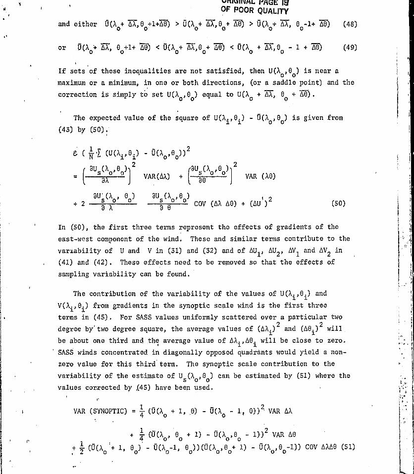
and either "0(a0+ Aa,00+1+A6) > U(X°* X, e0+ A) > U(Xa+ TA, 60_ I+ e) (48)or U(a0+ A 0 A0 < U(X0+ ZT,00+ 66) < U(a0 + Aa,00 - 1 + Qe) (49)

4

If sets of these inequalities are not satisfied, then U(A0 ,00) is near a

maximum or a minimum, in one or both directions, (or a saddle point) and the

correction is simply to set U(A 0 ,00) equal to U(a 0 + Aa, e0 + A8).

The expected value of the square of U(X i ,ei) - U(TO ,00) is given from

(43) by (50)

e. ( N 'Y (U (xi , e i) - 6(X0,60))2

r au2 au (X ,e)

2

s a^°^e0 VAR(Aa). + ae ° ° , VAR (a8)8U' (X , 0) 8U (X ' 0 )

+ 2 S °s

e° ° COV (AX A0) + (AU I ) 2 (50)

In (50), the first three terms represent the effects of gradients of the

east-west component of the wind. These and similar terms contribute to the

variability of U and V in (31) and (32) and of AU 11 AU2 , AV1 and AV2 in

(41) and (42). These effects need to be removed so that the effects of

sampling variability can be found.

The contribution of the variability of the values of U(X i ,e i) and

V(xi,ei) from gradients in the synoptic scale wind is the first three

terms in (45). For SASS values uniformly scattered over a particular two

degree by'two degree square, the average values of (AX i) 2 and (A0 i ) 2 will,

be about one third and the average value of AX i ,Ae i will be close to zero.

SASS winds concentrated in diagonally opposed quadrants would yield a non-

zero value for this third term. The synoptic scale contribution to the

variability of the estimate of U S (AO ,eo) can be estimated by (51) where the

values corrected by ,(45) have been used.

VAR (SYNOPTIC) = 4 (U(ab + 1 '. e) - 0(a0 - 1 ; 0)) 2• VAR AX

,.,

+ 4 (U ( X0 , e0 + 1) - U (;k , e0 - M 2 VAR A0

2 (U(a0 ' + 1, eo)

60 0-1, 00))(u(a0 ,e0+ 1) - 5(a0 , e

0-1)) COV Aa ee (51)

A

a

if

t

^ T 1 1

fD

.

The variability of the estimate, 0(?L0 , 80), fliat is the result of

mesoscale variability of the winds groin one SASS cell to the othor.and

of the effects of communication noise is found by means of (52).

4

VAR (MESO PLUS COMMUNICATION NOISL)

(AU 1 )

2 + (AU2 ).2 - VAR (SYNOPTIC)

(AU^) 2 (52)

where (AU) is now defined in (43) by equation (52). Since VAR(SYNOPTIC,)

is an estimate, it may exceed (AU 1 ) 2 + (AU2 ) 2 in which case (AU ' ) 2 is set

to zero. -The analyses of superobservations by Pierson (1982, 1983) assumed

that gradients of the synoptic scale wind could be neglected in the study

of superobservations. For some parts of the wind fields obtained from the

SASS, the assumption is not justified, and this correction needs to be made.,

Often it is small. Specific examples will be given later.

_A_ parallel set of equations for the north-south, components of thef

synoptic scale winds can also be obtained. The final results of processing

the data in this way produces values of U(X 0 ,00), V(X0 ,eo), AU and AV M at

the. integer values of A and 0 in the main part of the SASS swath where Aa

are Ae small. Near the edges of the SASS swath, which will be discussed

separately, other methods are needed because of the smaller number of values

in the sunerobservation, the location of the data fairly far from the desired

latitude and longitude and the lack of values for all of the quantities

needed in the above equations.4

f

The elliptical scatter of the winds that form a superobservation is an

important aspect of the sampling variability of the measurements. From (52),

and its equivalent for V and from (35), (36), (37) aid (38), reduced values

of AU '1 and AU may prove useful in studying the effects of mesoscale

variability and communication noise.

Let

K _ l( AU ) 2 + (AV') 2) [(AU

I) 2 + (AU

2 ) 2 + (AV1 ) 2 + (AV 2)21-1

(53)

t

f

F

ii

^^ a

^^ 9

io

E,

Then let QUA = K^j AU 1

AU; - 0 AU

v, - Kiz AVl

AV2 = K b' AV2

ORIGINAL. PACOF POOR QUALITY (54)

(55)

(56)

(57)

4

,This change effectively reduces the elliptical scatter of the original data

by an amount attributable to the removal of synoptic scale variability over

the two degree by two degree square.

The final result of the steps taken so far is to make it possible to

represent the east-west and north-south components of the synoptic scale

wind at X0,6o in forms similar to equations (19) and (21). They are

equations (58) and (59) and equations (60) and (61) .

01 10 ) U s ( a0 , e0) + t 1 tJr`Z AU + t2 N `_z QU2 (58)

V(a0 , e0) Vs (X0 ,e0) + t 1N`^ QV i + t2 N-h AV2 (59)

Cis (a0 ,eo) = U(a0 ,e0) - t l N x L1Ux - t2 N ' Qu2 (60)

Vs ( a0 , eo) V(a0 ,e0) - t• 1 N -h AV - t2 N -1-2 QV2 (61)

For an analysis of (58) and (59), the same values for t and t 2 must

be used in both equations. This shows that U and V are not independent and

for example that

8 f ( (0 (Xo' eo) ` Us (Xo' eo ^V(Xo' eo) ` Vs (X ) eo ) (62)

NT1 (AU' L1V1 H AU;AV2) (63)

a ,

Equations (60) and (61) put all of the lk.'known statistics on the right

hand side., , It needs to be interpreted with care. There is, conceptually,

only ono correct value for U s , and only one, for Vs . Picking t1 and t2 at

random generates many values of U s and Vs , one of which may be the correct

one. It tl°and t2 are constrained to lie on a circle and are normally

R

s,<

P.A•

t^ w

i

4 x

t

j(

E

A

f

pp`,^( ^y q

pi n

n^ i},,

`, ^ yx j F lR Y 4 4 ^YY^SM1^Y ^M w`. •^^^?w^. U'`^

YOF POOR QUAD. TY

2

distributed then

t 2 2P0 t2 2^1 j e`(tI * t2)/2

Qt + t2

dt1 dt2

f

1 2Tr a"t2

/2^d^d0fR

^O2Tr

o

^-fi2/2e

so that if R [ 2, the ellipse generated in the Us

Vs plane will have a

probability of 0,865 of enclosing the true value of U s and s

In t;he analysis of superobservations, each SASS wind in the four

degree square is given equal weight, in contrast to some of the present

'k analysis techniques that weight wind and pressure reports from ships as

a function of how far away they are from the grid point being analysed.

For ccnventional data and conventional analysis procedvri<s, the same

.^ report will influence a n,.id a„t from

: ,,t fej--.--- ^j +. potr.aaV .4^^3m de4^^7VR#ic i Da^ ,A.Rr away as .4iyG

or ten degrees of latitude or longitude. Other sources of error

dominate the analysis of conventional data and maximum use must be

made of each oceanic observation because of the poor spacing and

sparceness of the data.

For SASS data the error sources are different and the dominant ones

are essentially random-,, Equally weighted observations are the most

effective way to reduce the variability inherent in the SASS data,

,s

a ,

a

i

A ,

A

n

k ll

Sc E

,r1

fl

r

r

a

A

1

1

i

e „ ^: n M

i

x ^fitpe• j ^ ' u

3 «6 ^

N

+ O

1

i

}

THE FIELD OF HORIZONTAL DiVhRGUNCH

For constant density at a fixed height above the sea surface, the

eq,^iation of continuity in spherical coordinates is given by equation (64),

d,d

l ( 1 1 au i a (cos OV = 0 (64)aN J cos cos 0 57 TO

The divorgence`of the horizontal wind at 19.5 meters for a neutral

atmosphere is given by equation (65).

dlvIV R

Mau cos 0 sin 8 Vl (65)Rcos 62 h ( Be J

A finite difference estimate of the divergence at a one degree resolution

requires values of U at X+ 1, 00 and A , I, 60 and values of V at A0 , 0 + 1;t X0, e0 and X0, 00 - 1. We neglect also the ellipticity of the Barth, and

use R = 2.10 7 (n)" l . The equations are in the form, of (60) and" C61).

The finite difference value for the horizontal divergence of the wind

is given by equation (66) where the various AU1 , and so on, are associated

with the appropriate latitude and longitude.r

/

^div =v Is_4.5.10-

6 (OCA +1 0) -t AU K t ^U ; -U(a 0)2

h

_ cos eo 0 ' 0 1 1 - 2 2 0- ' o

+ t3 U1 + t4 AU2l11

+ cos 0O [V(A0) 00 + 1) - is AV - t6 AV2

k 1

V(a0' 00 -1) + t7 AV; + tg AV; - 0.0349065 sin e(V(X

0 ,00 )..JJ

- t9 AV I. - t10' AV2) (66)

The expected value of (div2 IVh)s simplifies to equation (67)

• 4,5,10-6 •

(diV2 IV;h ) 8 = cos 0 t(^'0

+ 1, 00 ) - U ( a0 - 1, 00) .

oIr

+ cos eo (v(? o , eo + 1) - v(x0 , 00 - 1))

- 0.0349065 (sin a V(Xo , 0031 y= d9.v2 \Vh (67)

kt ,^

r

F

^:^.r q,..,m«^ xx^ _. _... o nu -..yna.. s. a ., ..... ^... ..a -. ,.....w.. ,.w. ,.^,. +-k.,-.. .. ....-r..-. ...w — ,.. ..:« w .^ :.......__. ... fir. .._.... -n *:.. Ff '#A • .k_ sr,

k

ORIGINAL PAGE ISOF POOR QUALITY

The expected value of the variance of the divergence is given by equation (68)

2e, ((div, W. ) s ~ (da.v2 ^Yh ) ) , VAR (div, ^V11)

11• 2.025

(AU1 (Xo + 1, 80))2 .^ ( AUZ(a0 + x , 00)) 2 + (AU1(Xo_1,00))2(cos 00)

+(AU2(ao -'1, 00)) * (cos 00 ) 2 ((AV (Xo , 0o + 1)) 2 + (AV2 (XQ , 00 * l))2

+ (AV1(X0 ,00 - 1)) 2 + (AV ' o , 00.. 1))2)

+ 1..2184 . 10" (sin 0e ) 2 ((AVl (ae,00)) 2 + (AV2(ae , 00)) 2 ) (68)

The divergence at one of the grid points in the SASS swath whore

sufficient data are available is thus given by equation (69) where t by

the central limit theorem is approximately a normally distributed random

variable with a zero mean and a unit variance.

(div2 IVh) s

di^ v2 W. + t (VAR(divv )) f (69)

The wind in the layer of air near the ocean surface can be expressed

as a functiont of height, h, given the wind profile for the first few

hundred meters. Given the friction velocity, (tit *), the divergence can be

expressed as a function of height for neutra: stability and integrated

from the surface upward. This will be done after the fields for the wind

stress and the curl of the wind stress are found.

e

I

J ^

t 1

[ t

f•

4r

1[ f

ti

1

^Q

f

J6

f,

t

. .: 1

r

j t ,

JW

j r BOUNDARY LAYER AND WIND STRESS

The Monin-Obukhov theory and the concept of the drag coefficient given

' by equation (70) for a neutral atmosphere

CD10 u*/UlU(70)

J where u* z r/p = - <urw^ '> (71)

1f have been the methods used to try to understand the turbulent boundary layer

over the ocean. Many different sets of measurements have been made in order

to try to determine the relationship between wind stress and the wind at 10

meters.

It is not relevant to this particular investigation to review the great

Many papers that have been written that describe the results of these many

investigations. Reviews of some of these studies are given by Phillips (1977)

and Neumann and Pierson (1966).

More recent results using more modern and more carefully calibrated

instrumentation that cover a large range of wind speeds are those of

Davidson, et al. (1981).nittmer (1977), Smith (1980) and Large and Pond (1981).

Low winds are covered by Davidson, et al. (1981), low and moderate winds, by

Dittmer (1977) and moderate and high winds, by Smith (1980) and Large and

Pond (1981) .

Smith and Large and Pond used methods that measured <u^w^> directly as

well as the dissipation in the Kolmogorov range which was than correlatedr

wii:h <u w,> ind U10 . All of the data obtained to determine the relationship

between wind stress and U 10 scatter when plotted either as T/p versus U10

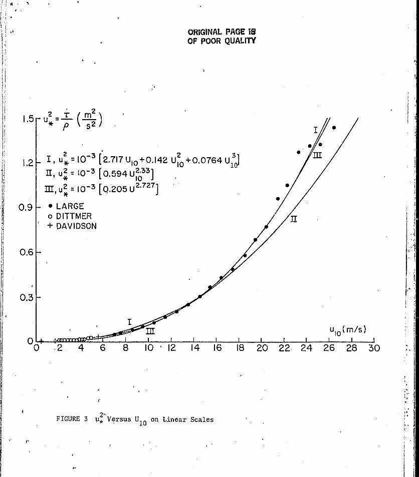
or as C 10 versus U10'

To investigate the problem in still one more way, an analysis was'made

as a term paper by Vera, of the data provided by W. G. Large and extracted

from the publications of Davidson, et al. and Aittmer. For neutral stability,

the data i4ere of the form n i l CT/p)i' U10i, for a data set that ranged from

light winds,of 1 m/s to winds of 27 m/s. The higher winds have smaller values

r

Vera, Emilio E., A Study of Curve Fitting Procedure for the Wind VersusWind Stress Relationship. Term paper for an Oceanography Course, The CityCollege of New York.

a :'

k

.y

t

M"

A4001L 4L

i?

Et

t

for ni (where ni represented the number of individual runs in a restricted

. range of wind speeds that were averaged to produce the u* and U 10 values)

and weight the fit less strongly than moderate and low wands.

he-need is for the most accurate possible predict on of the wind stress

given the wand at ten meters. Instead of first finding C 10 , it seems that it

would be more direct to-minimize the error in predicting the wand stress from

the wind speed from the available data as in equation (72).

NQ = J(na(T /P) i " A U 10i = B

U20i ^ C U30i)2 (72)

This is accomplished by finding those values of A, B and C t,tat minimize Q

by requiring that 8Q/9A = 0 aQ/8B = 0 and 8Q/DC = 0 which yields equations

(73) .

ni U1Oi Ini UlOi ^ n a UIOi A I ni U10i (T/P)i

cc 5 2L n i U10i ^ ni UlOi Yn i U 10i B Y n i. U lOi (T/P) i

ni U10i Xn i UIOi In i U10i C ni UlOi (T/P) i (73)

A good fit was found for the data that were used in terms of equation (74).

u2 = T/p = 10 -3 (2:717 U10 + 0.142 U10 + 0.0761 U1 0) (74)

, Graphs of T/p versus U 10 for the averaged data •of Large and as extracted

from the two other sources are plotted on linear scales in Figure 3 and on

logarithmic scales in Figure 4. Figure 4 shows how the slope of the T/p versus

U10 relationship varies from one-to almost three as the wind speed increases.

Vera also investigated the possibility that some power law as in equation

(75) might,-fit the data better.

1.

T/p = au.R (75)

a" It was found that no power law did as well as equation (74). As shown in

N4^

f

3e t

i

I

,o

A`i

i

. r Figure 4 power laws can only be made to fit a portion of the data and Fail

outside of a restricted range. Equation (74) will consequently be ut;ed in

this investigation subj Ict to the comment made in the introduction. Given

any equation teat relates wind stress and the wind at ten meters, the

• analysis that follows can still be applied.is l

The SASS data are for winds at 19.5 meters. To calculate the stress it

is necessary to r know the wind at 10 meters. The wand at 10 meters is^z

u* (U10)f

U(10) ^n (10/zo) (76)

i

r^ ,since u* (U10 ) is known as a function of U 10 , which implies zo , and at 1,x+.5

rAII meters it 'isE

uk(U)U(19.5) = -----K10 On (19.5/z o) (77)

so that

U(19.5) U(10) + ui^(U

10) za (19.5/10) (78)

When U(10) is varied ire convenient increments, a table of U(19.5) versus U(10)

can be generated. Given a value of U(19.5), interpolation yields a value of

U(10) to be in the calculation of T/p and if p is known T.

r^

4

a ^

I.

r.r

t1

t

t^^

n

a x.. _: e

9 i

7S i ,

ORIGINAL PAGE 15OF POOR QUALITY

i

R

aa

rp

1.52

_ .._.u2 - T

mS2

1.2 3 s u2 = 10-3

a [2.717 U +0.142 U Z^© i© +0.0764 U sl

0

II, u* 1 0 -3 .0,594 U o 31•'.r III, u2 = 10 -3

2.7271[Q.205 UA

•` 0.9 • LARGE. o D ITTMER

+ DAVIDSON

i4 0.6

I 0.3 F•

'. u^o(m/S) s0 i

,r

0 .2 4 6 8 10 r 12 14 16 18 20 22 24 26 28 30

r

r-y...

1Y1IIII

r

.

'

,'r

r

t^

t

.

21,

FIGURE 3 u* Versus U lQ one Linear Scales

V,`

k.

r•

i

P

W , I

P'

f

3 ^ '

'^

I1

vMUINAL PACE F

2 _ T M 2 OF POOR QUALrry2.0 U* .. ^..rr.r

I;5 S2

1.0 I

LARGE ^ l0M 3

• •0.5 ^ DITTMER

+ DAVIDSON, et of

(U^

10

0.1

0.05

r'

r

i

3 '

1

i

t^ •

L- s

Nu10

^Li H

0.1

H/ /UrMMK-

.f'

i

Y

0.5 I 2 3 4 5 6 78910 15 202530

FIGURE 4 u Versus U10 on logarithmic Scales.

P

t

r

ORIGINALTHE CALCULATION OF THE STRESS PACE FSOF POOR PACE

Giveii the individual SASS winds scattered over a SEASAT swath, one

might, , consider taking the basic data reducing the wind to 10 m., calcu-

lating the stress and deriving such quantities as the curl of the stress at

whateVer resolution is available. For many reasons, this line of analysis

will lead to dubious results.

Aspects of.the difficulty can be illustrated by calculating a super-

observation wind stress two different ways,. The first .i,s by calculating the

stress at each SASS point averaging the stresses, and analysing the

statistics, and the second is by'using the results of equations (5) to (10),

reinterpreting them and calculating the stress and its statistics from the

vector averaged winds.

A new coordinate System is needed as a first step. Let two great circles

Al intersect at X , 6with one .in the direction X from (5) and the other at,0 0right angles to it, and let distance along the first be given by G (degrees)

and along the second by G 2 (degrees). A coordinate transformation would be

possible as in the divergence analysis as a last step when needed.

The wind from the SASS at any point in the two degree by two degree

square would then be represented by (79) and (80).

V U (Xi.9 e AU (79)Pi P i i

VNi VN (li ,li ) + AV- (80)

where in turn

9 U(X ' 8 @U (}gyp , 60)0 0)

AUDG

AG li + DG

AG 2i

2

} : + tli

'AU+ t2i

AUc(81)

I m

and-3V(x

AV 0 0 0 0AG. AG

li 2i@GM1 2

+ t AV + t AV (82)3i . 4i, 3m

Mr--

too

u

1tt

l

ii

41

/"L" Y

OF pOop^In (81) and (82).any residuals from the gradients of the wind from the

average values of AG li and AG 2ican be removed for superobservations as

shown by ©quation (44). The terms AU m, AUc , AVM and AVc have a new meaning

and must be interpreted in terms of the analysis given by Pierson (1982).

The terms, AU and AVm, represent the contribution to a particular SASS wind

of the mesoscale variability of the wind for each SASS cell. The terms, AU

and AV , represent the communication noise error in the measurement made by

SASS for each pair of cells. They are in the form of standard deviations to

be multiplied by random numbers-, t li , t2i , t31 , and t4i , from zero mean unit

variance probability density functions. This random error is a not too well

known function of incidence angle, aspect angle, polarization and neutral

stability wind speed. For winds near upwind, downwind and crass wand, the

communication noise error can be substantial and the mesoscale contribution

is a strong function of wind speed. If finite differences are used to

calculate divergences over smaller distances with the original SASS winds, the

last two terms in (81) and (82) dominate the calculation of the gradients to

find differences as opposed to the analysis given previously for a superobser-

vations. The SASS GOASEX data do not provide a way to separate these two

effects. Even more discouraging.results are obtained when these individual

observations are used to obtain wind ;tress and wind stress curl.

From (79) and (80), the magnitude of the wind at a i 0 i is

i

IVi l ((Up(Xi)0 i) + AUi ) 2 + (AV i ) 2 ) 2 (83)

r

and so the magnitude of T/p is

i.:

c

1

T/P (Xi $ e i) = AIVi l t BlV i l 2 + C,V il 3 (84)

When expanded to second order in. AUi and AVi ,-this becomes (85)

T/P (ai'0i) = AUF ( a i3O i) + B (Up(X i3O i)) 2 +'C (UP (Xi'0il)3

i (A + 2BUp ( X i, e i). + 3C (Up( X i' 6 i) ) 2 ) U

+ (B + 3CUP(Xi$ ei)) (AUi) 21

,

+ (B + 2 CU P (X i ,ei))(Avi)2 (85)

. k .._}

U

^T!r ^

r `

t

}if

tf

a^

ORIGINAL PAGE F

OF POOR QUALITY

4

The squares of AU. and AV i involve terms of the form,3.

t 2 (.QUM) 2 + t2 i (AU c) 2

that Flo not :Fluctuate about zero and that do not average to zero.

Moreover they are amplified at high-winds by the wind speed. Individual

values of the wind stress calculated from the SASS data thus appear to be

somewhat untrustworthy.R

If the N winds used to generate the superobservation wind are each

used separately, N values of T/p can be obtained and these N magnitudes

of T/p can be averaged. The expected value of this average is given by

(86) where, U = U(X0 , 60 ) .

(T/p(ai,6i)) = AGP + BU 22 + CUP

au au(A +' 2BUP + 3CUp) (^GP QG1 +

aGP C1G2)

1 2DO z au 2 Wau

+ (B+3CUp) 2 ( (aG P)

VAR AG + ( aGP ) VARAG2 aG* 2P aGP

COV AG AG 2)1 2 1 2

av 2 aV 2 aV aV+ (B+2 UP ) 2 (( aG P) VAR AGl + ( aGP) VARAG2 +

2 2 aGP COV AGl AG2)

1 2 1 2

au av au av aG av

+ (B+3CUp)(B+ 2 UP)( aGP aG

2P VARAGl

2+ aGP aGP

2

VAR AG2 + aGP

1 aG

2^

' l

DO aVp

+ DG aG ) COV AG1 AG2

2 1

+ (AU m) 2 + (AU C) 2 + (AV m) 2 + (AV c) 2 (86)

41though the average can in theory be corrected by various estimates of

the numerous terms that produce a bias, the errors of various kinds in the

original SASS data are quite large. Additional terms to third order would

introduce,even larger effects since the cube of the wind speed is involved.

Variability in direction produces even more intricate results.

The variance of the data would be found from g (T/p (Xi,e i) - T/R (Xi$Oi))2

and yields terms involving the squares of AUm, AUc , AVM and AV multiplied

E

a

i

n

fi

i

r

!'W ea

NaY

,^ 9

...^... -^. _ ,r... - rte .., , u.. ___f^.a .. w . „ya.n 1. 3,.au.3aar ..r.a+:..

MALI L46V

dRIGINAL PAGE 13

fClFprky+' . ' OF POOR QUALITY

511 4

f r

Functions of U, A, B and C. This variance would be reduced by N^ when used

4 ^. in calculations involving the wind stress field but proceeding in this way

leads to intricate correction procedures and the need to correct for large

# effects.

In contrast consider the average wand for the N values around X o, 00 as

given by (29) and (30) • which could be corrected for the effects of a gradient r

{ by finding (45) and its counterpart for V(a0 ,O0). The standard deviations

is caused only by the combined effects of mesoscale effects and communication

i noise could be found from (54) through (57) and returning to vectors parallel

t1

and normal to the directs on

{ The result would be four numbers atao , 0 0, namely j(, anda

{

VP = UP(X 00) + t5 N7' 2 vu (87)o ,

4

{:e

t ivN t6 N_^

AV (88)(88)

where the combined residual effects of mesoscale variability and communication

t noise have been reduced by N l to describe the sampling variability of the

mean. Failure to correct for the contribution from the synoptic scale

^j' gradients and using the values found at Xo + AX, 00 + AX with standard%deviations reduced by N^z would also give much more stable results.

,. For a superobservation, substitute (87) and (88) into (85) and the {

result is '89).

T/ p ( 6o) s = AUP + BO + CUP

SEi

+ (A + 2BU P + 3CUp) t5N _

AUmc++

^•

2+ (B + 3CUp) is

N-1 (AU

MC)

1

,Y

+ (B + 2 CUP) t2 N -1 (Avmc ) 2 (89)

nb

#r

ti

Over one degree :field the uncertainty in the value of T/p(X00) is

A

o ,

greatly , reduced by the factor N_4 and the bias is even more strongly reduced

A

by N 'Similar effects occur for direction.

91

{

Y

ORIGINAL ij°^a^^' IanOF POOR QUALITY

r

It appears to suffice to process the data in an even simpler way for the

center of the swath. The superobservation wand data can be reduced to 10

meters instead of the individual winds. The value of U* = T/P(Xo ,60) can be

found from

' /P (x0 , 00 ; Up) = A Up + b 02 + C 03P

The variability of the stress in the direction X can be found from (27), (31.)

and (30) after correction by (54) to (57) and after correction to 10 meters,

Ap(T/P) = T/P ( Up + N ' z AU MC)- T/P (Up) (91)

The variability normal to R that would give a vector stress with the

same direction as the vector sum of (87) and (88) with t 5 = 0 and t 6 = 1

is given by (92)

N--2 AV

AN (T /P) = T/P( Up) ( MC ) (92)D

The stress is represented by

T/ p l ( xo , e0) Ps = T/P(Up) + t7 Ap( T /P) (93)

T/P(xo,eo)Ns = t 8 AN (T/P) (94)

with orthogonal components in the direction, R and normal to R. These in

turn can be resolved into east-west and north-south components and processed

in,the same way as the winds. "

s

a

i

r•

3

I DlF

1

i

r

r

w•f AL

-

THE CURL OF THE WIND STRESS ORIGx1NA7.1, 11'1`iOF POOR QUALITY

EThe curl of the horizontal vector wind stress is found by first multi.-4 ^1

'.! plying equatr,ons (93) and (94) by p (/1O 0 00 ) which can be found from the airH temperature and the atmospheric pressure at the sea surface and then computing

the north-south and east-west components of the stress plus the appropriatet /TIC. vn7ua.G of ofa _A ) vary nhnut 7.25 kv/m rn nnherical enordinates.

r

j

DT 8 (COS eT{ CURL (Th)= 1r cRs e ( 8._

a e (X)s

r }cos a TMs

u TMs

R ( a- cos e a e +sin 8 T (M)s ) (95)

where T (e)s and T(N)s are the north-south and east-west vector components of

M Ts. If for example

T (6) s o e o o 0 9 1 l0 2) = T. (^ ,e ) + t AT + t AT (96)l,e)

T (J^(a) s o ' eo M) =T (a

o,e

0 11 3 12) +t AT +t AT 4 (97)

and soon, the finite difference value of (95) is

6

CURL (T) _ 4.5 . 10 -(T (^ , 1, e) - T (^ - 1 e )

h s- (cos e) t (e) s0

- cos e (T (M)s (Xo, 0 + 1) - T(M)s (X0, 0 - 1)

+ 0.0349065 sin 0 TM s (xo' eo)

)J

(98)

with dimensions of (newtons m-2 -1) m,

Ten different random effects are found in the calculation. The

expected value of the,curl and the expected value of the variance of the

curl are given by (99) and (100) where ten different AT's from the five

c different stresses that are used are needed for (100).

{ trr

1.

1

a•

{

k

i

,F

a 7

i

3

li" E

CA

{

ww`

r 1

.^e.. _.... ...^-.,. ssm^mm..-.<... .. a ... ,..

II

I

ORIGINAL PAC.;a jaOF POOR QUALITY

e (CURL (Th

4.5-10"6, 0

1 i (N + 1 0 0 - 1 0(0) 0 0 (0) 0

(Cos 00)

cos 00 (TM (X0 , 00 + 1) - T ( Xo s oo 1))

sr•

+ 0,0349065 sin e T (X '0 M 00 0

CURL(99)h

VAR (CURL(T+ h

1,0252-- 0

+ 1, 00) 2 ) 2

(cos 00

+ 2 2(AT(X 11 0 + (AT(X - 1, 0 )

0 0 1 0 0 2

+ (cos 0) 2 WT^ 2(Xo,00 + 1) 3) +

+ -3 2 + (100)1.2184-10 (sin 00)2

((AT(X 0 0 0) 1

where the represents the additional terms needed to complete the

full equation,

so that

=(CURL T'h s CURL(,Ir*h) + t (VAR (rURLC'h

(101)

I

J1

II

^MI

6V•' SYNOPTIC SCALE VERTICAL VELOCITIES OrJG114A

3{If the neutral. wind profile is assumed to extend to the height, h2,

equation (6S) can be rewritten and the result integrated from h l , very near

the sea surface where W(Ro + h l) is nearly zero at the synoptic scale, to 112.

In the limit, h l can be set to zero dnd the subcript, 2, can be omitted,

tr

as Ro+}12 ('?o + h2(R2 {V (R ))dR = J

R div W dR (102)

Ro + Ill BR. Ro + hl 2 h

Many of the terms that arise and that enter into the finite difference

is calculation are negligible Two turn out to be important and are effectively

r multiplied by terms that are constants as far as the integration is concerned.

One is of the form given by equation (103).

2

(const l) dz = const l (h2 h l ) (103)

5hl

" t an6 the other is (104)!' Ei

pu} h2 h2 h1

const2 an(z/10) dzco'

'Ast2 ( 1 2 k 10 h2 ^ 11 1 an10 + h l ) (104)

h1i

By means of equations similar to (27), and following, with the wind

reduced to 10 meters and with the standard deviations of the means, valuesF ^^t for Vp , AU and AV can be round at ao , eo.

Define

u* = (Op + BV2 + CVp) (105)

Au*P = u* (Vp + AU) = u* (Vp) (106)

and' Au*N u* (Vp) - (AV/Vp) (107)

U* An z/ 1 0 AU* On Z/ 1 0Then Vp (z) s = I + + t1 (AU + ) (10$)

AUK Prn z/ 10VN(z)

s = t2 {AV + K ) (109)

1

f

n

F

P ' ♦ y

^.AR

1

0"n.

YlIt

- Ul0 (?o 1, Oo) 6 ^U (. 1, 00) ' on

10 '" 1 ,1 +t1 (AU1 + 62u*

(k 10 " 1)

4 J

r a

a a SJRiGINAL` 1' '1Ala Y

CAP POOR QUALITY,The terms analogous to (33) to (40) are

u* Cs^ (z/10)U ( Z) -(VP )sin XK

A« 0(10) + 6

i

U) On z/10

u(z/10)*

(110)

Vz x -(Vp + — K ) cos X

V(10) + (61V).2n (z/10) (111)

sin X Au*P an (z/10)

QU1 (z) = AU1 ..

AU +

( 62U1) fit ( z/10) (112)

co s X Au*N 3n (z/10)AU 2 (z) = AU2

_K

`AU2 + ( 62 U2 )an (z/10) (113)

cos R Au*P Dn (.z/10)'AV (z) ^ AV _

K

AV + ( 62V 1 ) Dn (z/10) (114)

sin X Au*N 2n (z/10)AV

(z) AV + K

AV + (62V2 k (z/10) (115)

The appropriate terms, all of which can be found for each grid point in

the ,field, can be substituted into (71). After integration of (102) and

simplification by the results implied by (103) and (104), the final result

is equation (116), where the subscript on h2 has been dropped. The AU's and

so on, need to be found at the correct latitudes and Longitudes.

A 6

t (h)s = 4.cos06 h U10 ( ^o + 1, O o ) + 6 1 1 + 1,80 ) (tin - l)

O0

,10

A.

,a

k

Yt

n

aeA .

1a 1s

v s '^'1 V^"6ey.stab "

,, n

W

E.?! n

r1

t

f • rf

+ t2 (AU2 + 62U2 (an 10 - 1)) - t3(AU1 + 62U 1 10

t n/y (rt! qqVV

rr^^^^,, NR

f^ a{; Vin.++

r

3 ^ ^Kt4 (AU2 + 62U2 10

1))^^(y ^u^

(2n-

+ cos (1^ (^, , 0 + 1) + d V(^ ,^ 0 1) (Qrt 11 - 1)o 10 1 10r 0 0 0 0

a?

V10(a0' ©0 1 1

X0 00 1) (%n 10 1) ^. .... •)

+ 0.0349065 sin 00(V10(X0'00)

......) (116)

{ At h = , 200 meters, M 10 - 1 is 2.0 and (117) becomes (118) in ms-1•

F ^W (200) = 9.10-0(N + 1, 0) + 2(d U(X + 1, @ )) + ...10s cos Oo 0 0 1 0 0

+ zos 60 (V10(a0,a0 + 1)

+ 2(6 1V(X0 ,a0 + 1) + ..,

+ 0.0349065 sin 00 (V10 (Xo' Oo)

+ 26lv(A0,00))

+ ....)J

(117)

,EAs in preceding analyses,

r ' w (200)= lu (200) + t Alu (200) (118)i

s

which can be evaluated in a way exactly similar to previous results.

As a note in passing, there is not much difference between (105), (106)

, and (T07) and (90) , (91) and (92) . The computation of error ^ for the

specific application is made simpler by the choice that was made. F7rom

11* + Au* = (u* + (Au* )) a = u * (I+ (Au*) /u*)

a•

= u* (1 + (Au*) / 2u*) = u* + ( Au*)/2u* (119)

it can be seen that two different ways to find Au * yield nearly the same

r quantity:r

r

a,

v

{

t • t

l^ M

fA,^

ib

r

a

INDEPENDENCE AND COVARIANCES

The reasons for the variability of one SASS pair of backscatter values

compared to another pair are basically uncorrelated and random. The mean

wind speed and the mean direction for a superobservation are perturbed by

two independent and uncorrelated random effects, one parallel to the wind

and one normal to it. A correlation becomes evident when resolving the super-

observation into east-west and north-south components. A superobservation has

been based on data from a 2 0 by '2° square, and once the effect of synoptic

scale gradients are removed (which involves SASS values scattered randomly

over the square from as far away as A° i 2 and e0

t 2), the estimate of

the standard deviation of the mean is based on a sample of independent random

variables. The choice of grid point spacing for superobservations for

future systems remain a matter to be investigated and is a function of the

model to be used and of the scatterometer that obtained the data. A

very coarse resolution model in the horizontal would require a more careful

treatment of gradients.

The use of overlapping squares at a one degree resolution introduces.

correlations between the estimates of the winds and the standard deviation

of the variability simply because the same values are used in different

estimates. Every other grid point in the east-west or north-south direction

is independent and those located diagonally (for example, X 0 ,00 to "0+1, 00+1)

are weakly correlated. Smoothness in the wind field can be judged by

inspecting every other point in the grid.

For the calculation of the divergence, the vertical velocity at h and

the curl of the wind stress, the analysis becomes more complex. Some

particular SASS speeds and, directions can make contributions to the means

plus standard deviations of three of the five terms that enter into the

calculation. (The additional complexity introduced by (45) is not considered).

Equations.(69) and (1.18) are essentially statistics formed from a linear

weighted combination of the original data. Equation (100) is a pseudo-t

linearized plus non linear weighted combination ,of the original data.

i

f

a

a

i

I

{

M'

j^

i

M`+

b ,^w

k

c

r '.

14

Correlations do not do much damage in the estimation of means, but they

can affect estimates of variances and standard deviations. The contribution

of a particular SASS value to the final estimate of the divergence can be

traced through the entire analysis. The value for the difference between two

estimates-of the east-west component so as to find 8U/ M is calculated from

completely different east-west components of the SASS values ane. thus the

numbers on which the estimate is based are independent. The north-south

difference so as to find BV/DO is based on completely different north-south

components of the SASS values weighed by a cosine and are also found from

completely different values and thus the estimate is based on independent data,

For the calculation of the divergence as in (69) and quantities such as

(101) and (119), the full expression is, however, somewhat more complicated

and merits a more complete analysis. In figure 4,the one degree squares that

contain SASS values that enter into t;te evaluation of (74) are numbered from

one to twelve. The values of U (X 0 ,00) and V (X0 ,00) (and so on) are

partially obtained from SASS values in squares 4, 5, 8, and 9. The wind for

the point, X . 0 . was represented by equation0. 0- s (60) and (61). bet N equal

N = N4 + N5 + N8 + N9 , and then the term t i AU' can be represented by (120).1

N

4 5 8

N N N

9t i AU1 ^'

ti,4 AU1 4 + ^t 5 AUl 5 + ti 8 AU1 8 + ^ ti 9AU1 ,09

(120)1 1 1 1 1

i^

{:_

where the is on the RHS are independent and the second subscript represents

the one degree square containing the SASS value. The expected value of each

side is zero and the expected value of the square of each side is

N4 N5 N8 N9 2C ( t 1 ^ 4 AU 1,4 + t1'5 AU1'5 • + t 1 ^ 8 AU 1,8 + ^ t

1,9 AU 1'9), 1 1 1 1

2' 4 (4 (AU1)) (121)

J

where the assumption that the error properties are the same in all four

squares is made.

All . of the contributions from each of the squares numbered in Vigure 1

can be identified by a double subscript notation as above. The analysis can

`f

{

j 1

4

a 9 a

i f+^`. yax

F a

p

^,

to p..

ae

j V

st

'r a.

^^ 1

0W`• Jy +M'!iJtGiikBk¢E7

be carried through keeping track of the dependence of AU. and AVl and of AU ' and AV2 throughout the finite difference calculation. ~

The contribution to -the divergence from squares, 4, 5, 8 and 9 come

from terms involving the gradi ents of Us and Vs and value of V s at a0, go.

{ For the AUa and AV1 terms in (60) and (61) a part of their contribution

can be represented by (122) where a is the coefficient of the sine term

in (67) .°

Contribution = t N (AU + cos 8 AV r a sin e AV )z

I ' S 5 1,5 0 1,5 0 1,5

+ t1,4 N9(AUl ^ g - cos e0 AV1 ^ 9 + a sin 00 AV1,9)

id

+ t1,4 N4

(-Au 1,.,4 + cos 60

AV 1,4 + a sin e0

AV 1,4)

+N8 ^ (-AU1 ^ 8'- cos 80

AV 1 ^ 8 + a^ sin e0 AV1 ^ 8) (122),8

° The expected value of this contribution to the divergence is zero. The

expected value of tl 5' t1 9 , t

l 4 and t2 8

are one. The squares of the

terms in parentheses give the terms found in (73) subject to the reasonable

assumption of (121) and what it implies plus twelve cross product terms.

The signs of the cross products terms are such that two of four similar terms

have positive signs and two have negative signs. The cross correlation

between U and V when estiamted from scattered SASS values will consequently,

cancel out and be close to zero in the estimate of the variability of the

' divergences as in (73). Although the terms in (71) as identified by t 1 to

t10) are not strictly independent, this analysis shows that (68) and consequently

(69), is essentially correct. The same conclusions are also valid for (99),

(100), (101), (116), (117) and (118),

a

°

¢

}

( ;y

P Y,d Y

.x

K 4^zb '^`b.

k

,

. ~

(|^i|

.^

,

. `

19

OF POOR QUALIV

^ ` .

,

'

'

^

Arrows' Fly with the Wind.

Barbs Proportional to Wind Sneod,

Full Barb Equals 10 m/s.

' .

. ^ .. . ^

'

- ^ `^ .

, ~ ./

..

IL

SASS

GOASEX

REV 1141

^^1

!. /-|

ORIGINAL PAGE IS

OF POOR QUALITY

010,Wk. A

19 18 SASS18 GOASEX

18 REV 1141

18

ININ

-0

18

18

1617

,1615

,r ,

PAGIIvOR 00A1-1 I "PO ,Of

<->

5.45

.45

,60. 50.55

.50

.4.45

.4o.40

35 .35

130.30 500

.25 .25

"^^,210 .20

.5

.10

.05 '4501v

.025

.025.05

rl

.025,

"o '.010

.025 ^ % ^ ^ '4p, N—^.

,.010

r/p U 2 2 .025(rivs)

.0!mognitude

direction

SASS I loGOASEX I If

REV 11 41 . 0,

ia

^r

«. e

t^ a

sknyf4.

1t. M

is ^' r '^ >11

f 41

n ,:

7]77^

1

r

i

zIj

i t1 r M .

3' r

Ik

1

a

,'op Left: SAMPLE SIZE

Top Right: VP

Bottom Loft: AV

Bottom Right: AV N

Multiply AV and AV

by N -h to get Standard

Deviations of the Mean.

t

v

r

ORIGINAL PAQE I.SOF P

OOR QUALITY

0 SASSP GU,>EX

PP^s P REV 1141

P/fig SF /^ P

I, 96 s /90 `^ P^?V'/OoF

x. / 9 9^5? 6 5

/22 66 ^^g /p 3^ 5 .^^ 19 4s+s s.8 1 5

one 3 g 9 2ps ^ Ig / 5.4

St0 / Z ^,• 3 S q

p 0'8 l9.40. 0 <0 6.8 g,p 9,^ 5/ 29 6,3X69 /3/ /.0 19,8 38

04 J ^^ 2^ 32 $ /0 /!Q 3 3A'' 19,R 32 5,4 18,5

3 ^4 Al ^ 3p 4.93 /' / ' I8,

20936 18.6 38 . 33

3 /•0" 35 4,9 1816 X 22/0 2,^ /8 0 0.8 18.30.9. 30 5,1 0-3.3 2, e 0 31 4.7

0 3,g J. 0 1,. 39

/' > /6/6 9 4 ^0 Imo- 7-^-.I 0-ft 33 0.9

G3 20 •0^ 4.032 ^/ o

.5 /82 2'9 ► 33S E

S? 3,0 p 28O99 33 2.6 0

X5.2 /'y. 30 3. I Soo0,7 .1407 1•9

&-!6-1 ' 2_^ 34

N! ^`- 15.9

0.8 3 2.0 ^- ---• i 91.6/r`'4 -5

0.8 15.5

2.5 o

! 0 10.7

40°N

1

r

30 -At

r

r'

F

{

j'^a`r(

i

SASSGOSEXREV 1183.

WIND (m/s)

Arrows fly with the Wind,

isarbs proportional to Wind

Speed.' Full Barb Equals

10 mks.

ORIGINAL PAGE ISOF POOR QUALITY

L

WOO

SO 0/v

J \y "'

35oM ^^ •^ ^`^'`^

2/0 0"c ~''1

s. ytNn

i a

I

A

ORIG NAL PAGE ITT

OF P OR QUALITY

^oso^

i

.. ppoF' 2.0 8

7/5.5 8r ,e' 3.0N4,3^T./ 1.4j /' /4„2 2.9 11 6.6/6.5 12/6.6

j

13/6.5 ^,0 Z j 5.3',7.5 14/4.6 }I 1,5/1.4 2,4,/4.4 q/ 0.4/8.4 +1.5/0.

03, a 2-5/10-70.4/1,314/12,3

0.40 6,7/ 10,E 0.33

' 1^ 0.92.7/1,635/104 20 2`Q04 12.3

3.1 / 1.8 5' a^^^;lr 28/67 32/14.1 ^' ti^ 0

b. %^.3 1.3/2.1 3a/la.l s.y1t,^6

4 211.08 12/293b112a v^'a

11/ 85 1A.2 9

3 7/13.3 2.6 8019'

5 1.0/1.7 33/13.335r/1^ I1. 2 10/9.62.0%2.0 32/125 • /9.

y§ 39« /13.0 I y 3.2/,0.3

017/115. 'S6/ 10.919/12's355/Iy7 2 .8 122/6.71.5/1,8, 0.6 /1.1 34/11.7 2'5/4,1

087 1.2%^ I 38/10.112113.0 •' / %I,I/1.4 3T^^I+A 1,4/181.45/6.6

0.9/1,4 35/10.7 1.8/16 ►7/1.2224/12,0 t.4 2.1

► nil 6 29/9,04411/.11.2 1,3/2.5 2.0/6.8

38/99 1.7/22F 10 /i1.6 1~+Ii/5 '500• 0,3/0.5 .6 25 /$.5 .•:2

«32/10.9 !,s 1.2/1.20.8/0,8 ! 5 19/5.7S! 2$/%5 2 I %1.4i(

1.0 /1.2 4./,3,811 /10.6

3r40'9/0.3

1, /30.81,5/1.0 JS/ J

2:-/.8. •6 !' b,6 8/291,7/1.4

' Top Left: SAMPLE; 2.5../,63

SIZE.,1^3 //88 .4

TOP Right: VP1,4/0.8 ,

Bottom Left: AV 2::5'3PBottom Right: AVN 12,7

0.9/1.0Multiply A. V and

A V by N-^ to get SASS fps'£N

G0ASEXStandard Deviations REV X83 ^s°N

Of the Mean.

7+'.0.7/0.4

1/3 .5

0.8/1.27/3.0

0-8/0-4 lo/3.T 0.8/1-2

7/5-3

14/2.60, 7/0.7 14/3,6

0.9/1.1 11/6.12 3.0

j4 ^pk 4

7'Poo"

545 / 'e.

334 01112

12

11 660 v10

.7 14

--9

8

9

10 8

11

12 137

5

500

4

10

8

SASS 54-

GOAS8X ISO

RE V i 16 2-1134 5 6

ii

v t

t

i

1

4

i

r'

ORIGIIVAL pAGLv it,OF POOR

QUALITY

S 4p 3`Sodo

M '+S

4

CO

dn7©

I

Arrows Fly with the Wind.

00

^ f 1

Barbs Proportional to Wind Speed.) J t

N / J o^ Full Barb Bc{uals 10 m/-s,

40 , / s0E

J

/ J

j j

WIND (m/s)3

SASS

GOASEX

j REV 1298

r^

z

i

1 ',^ d

:1

r'^ ^? E ^ 4 t t

t5•

1

z1 4

3 i

ii

Top Left; SAMPLE SIZE

Tap Right: V'p

Bottom Left: 'AVP

Bottom Right; AV

Multiply AV and AV

by N-h to got Standard

Deviations of the Mean.

.

i

Ar AVa

Y,

ORIGINAL PAGE 1g

OF p0OR QUALITY.

%p • tl'9a 1 SASS1.3/I.o10 GQASEX

1.4/ 1 REV 129836/10 3

1.3/1.91 4/13,7 30/9.3 .

3 7, I,E1/1 3 13/ ,6

3• 2 Qs2.8!1.000,

01" 6113

, /" 30/12.4 99/712-^733//^' 1.7/l.619/IL9,9/1,5

L/I.19l l 36/11, 119/1.8 10/10.2

34/6,5 Imo; ,4'13 /1,4 27/65

2,4/3.5

/ /S 9 /q^s 2 1,9 2815

01%s3 2 I.7j12 50.

0jis /sue U,9 1,2/3,9

!S tie/ ps^s2 0,8/0.8

8/4r r 'g r'^ pis ?iiq '"^ •0

a9 .,o 0

ts^_ 1 0 ,p 012 4.4

0,8/112dD

2^i

^^p^-3g 22/5,1

45°/v q^ v1.2/2 ,2 IZ/6,0

^° N o . ► 1,4/09L

:5;5,411/3.4 31/5.6

ILA i tD 1.2 / 1.0to N

•1 .. p .0 F

LA-,^s s 3L/4,4

Wz 1.7/1.5 \0153

NNAl\,3

115/9,2 of W i"o0

1.0/2.0 'a !3^X2.0133/6,2 ^

2.1/1.6 23/3,5 1.6/2.7

1.4/0.9 :15/2,20,4/10.4• •

F

^l

Y

ff

Solid Lines Isotachs

Dashed Lines Stream-lines.

N

ORIGINAL 11AUZ Nmc onno nt IM ITV

113 12 11 10 SASS

GOASEXREV 1298

9

9

13

12 5

4

00

510\ 6

_ 125_!OAf

10 5

4

9 8^ 71 1 5 14

.005

^' C^ 010 (^

.010."." ,P'. , U

. :8°^^`=-- .020

.050 .025 Q

'10,...050

04,

,15^-r

S o ,20

'.15 .050:10 1 — -- .025

7- ^..

.050 o ,\ '- --

050

7 'u^'p ^ 1 -^^ 0025

.025.02000

R

i. I.050

u* (M/S)21 1 --- ISOLINES

23.025/ ,^ I — -- DIRECTIONOp

.02 ^^ o ,010 SASS

1GOASEX

__. REV 1298

3 0, ' ^3

2 Sp^ 240.°E

.020 .020.

...

lf?IGINAL '^sF'

p00R QUALI'

N

x,

h

f,

Y

t

t

U

II

I`

lI

tFl^

,t

l^e

6

{^pyY

1

,

A

y.

'01GINAL PAGE fg-

IF Poon QUALI ry

a

IN

q I

11