Solution of the Radial Diffusivity Equation The radial diffusivity equation in dimensionless form is as follows (1) Our objective now is to solve eq. (1) by the help of the Laplace transform. The main advantage of the Laplace transform is that it enables one to express a partial differential equation D D D D D 2 D D 2 t P r P r 1 r P ∂ ∂ = ∂ ∂ × + ∂ ∂
Transcript
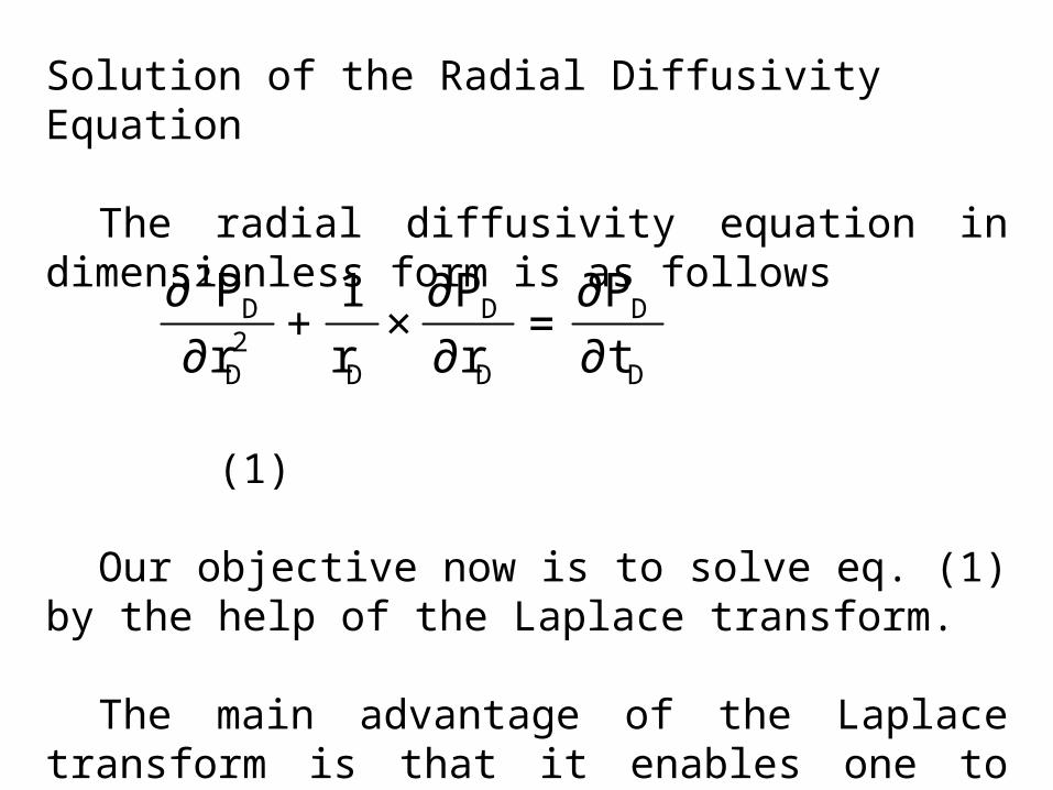
Solution of the Radial Diffusivity Equation
The radial diffusivity equation in dimensionless form is as follows
(1)
Our objective now is to solve eq. (1) by the help of the Laplace transform.
The main advantage of the Laplace transform is that it enables one to express a partial differential equation as a total differential equation. Therefore we can find
D
D
D
D
D2D
D2
t
P
r
P
r
1
r
P
∂
∂=
∂
∂×+
∂
∂
)0,r(P-Pz]t∂
P∂[L DDD
D
D = (2)
(3)
Because z is a parameter,
subject to the following conditions:
1. PD = 0, for tD = 0 at all rD
)]t,r(P[Lr∂
∂]
r∂
P∂[L DDD
DD
D =
)z,r(Pr∂
∂DD
D
=
D
DDDD
D dr
)z,r(dP)z,r(P
r∂
∂=
2. 1-)r∂
P∂( 1r
D
D
D== , for all tD > 0
3. for all tD
then the diffusivity equation in terms of Laplace domain is stated as:
(4)
subject to the following conditions:
1. , for tD = 0 at all rD (5)
0)r
P(
weDe r/rrD
D =∂
∂=
)0(P-)z(Pzdr
)z(Pd
r
1
dr
)z(PdDD
D
D
D2D
D2
=+
0)z(PD =
2. (6)
3. (7)
Applying condition 1 to eq. (4), we obtain
(8)
Eq. (8) is a form of Bessel’s equation. Its general solution is given by:
z/1-)dr
)z(Pd( 1r
D
D
D==
0)dr
)z(Pd(
weDe r/rrD
D==
)z(Pzdr
)z(Pd
r
1
dr
)z(PdD
D
D
D2D
D2
=+
(9)
where I0 (rD√z) and K0 (rD√z), respectively, are zero order modified Bessel functions of the first and second kind; and A and B are constants to be determined by applying boundary conditions 2 and 3.
From the properties of the Bessel functions, we have;
(d/drD)×[I0 (rD√z)] = √z I1 (rD√z)
and (d/drD)[K0(rD√z) = -√z K1 (rD√z)
)zr(BK)zr(AI)z(P D0D0D +=
where I1(rD√z), K1(rD√z) = modified first order Bessel functions of the first and second kind, respectively.
Now, we apply the boundary conditions eqs. (6) and (7) to eq. (9).
To apply the condition in eq. (6), we differentiate eq. (9) w.r.t rD, substituting rD = 1 and equate the result -1/z to obtain
A √z I1(√z) -B√z K1(√z) = - (1/z) (10)
A √z I1(rDe√z) -B√z K1(rDe√z) = 0 (11)
By multiplying both sides of eq. (10) by K1(rDe √z), and by multiplying both sides of eq. (11) by K1(√z) and then subtracting the resulting equations, we get
Likewise,
Substituting the values of A and B in eq. (9), we get
(12)
)]z(I)zr(K-)zr(I)z(K[z
)zr(KA
1De1De112/3
De1=
)]z(I)zr(K-)zr(I)z(K[z
)zr(IB
1De1De112/3
De1=
)]z(I)zr(K-)zr(I)z(K[z
)zr(K)zr(I)zr(I)zr(K)z(P
1De1De112/3
D0De1D0De1D
+=
Returning to eq. (9), we have
van Everdingen and Hurst argue that since , which is actually , is the transform of the pressure drop at a point in the drainage area, then by initial condition 1, Must be equal to zero at any point in the drainage area which has not yet been affected by the pressure drop at the well; which is another way of viewing the transient or infinite acting state.
From the characteristics of the Bessel functions, I0(rD√z) increases as rd increases and K0(rD√z) approaches zero.
)zr(BK)zr(AI)z(P D0D0D +=
)z(PD
)z,r(P DD
)z,r(P DD
Therefore, to adhere to the initial condition 1, the constant A in eq. (9) must be set equal to zero and the equation reduces to
(13)
By applying boundary condition 2, eq. (6), we get:
Since, then,
)zr(BK)z(P D0D =
z
1-)z(KzB)
dr
Pd( '
01rD
D
D===
)z(K-)z(K 1'0 =
)z(Kz
1B
12/3=
and eq. (13) becomes:
(14)
From the definition of the Laplace parameter, z, stated following equation
when tD is small, z is large. With z large,
for n ≥ 0
Thus, at rD = 1, eq. (14) becomes: (15)
)z(Kz
)zr(K)z(P
12/3
D0D =
∫∞
0
zt- dt)t(fe)]t(f[L =
z-n e)z2/()z(K π=
2/3D z
1)z(P =
Eq. (15) can be inverted by referring to a table of Laplace transforms. Thus,
(16)
Returning to eq. (14), we want to evaluate this equation when tD is large, i.e., when z is small. From the properties of Bessel functions, the following approximations can be made:
Thus, at rD = 1, eq. (14) becomes:
2/1DD t
2P
π=
)]2/z[ln(-≈)z(K0 γ
z/1≈)z(K1
2/3Dz
z]2
z[ln-
)z(P
γ
=
(17)
or,
The inverse Laplace transform of the first term is equal to ln(γtD)/2, where γ is Euler’s constant:
γ = 1.78107255, lnγ = 0.57721574
The second and third terms above are inverted according to . Thus,
PD = (1/2)[ln tD + 0.80908] (18)
z
2ln
z
ln-
z2
zln-)z(PD +
γ=
Also, eq. (18) is identical to eq. (4-17) when the skin factor, S, is set equal to zero.
Sometimes the pressure at the outer boundary of the drainage area of the well remains constant during the test.
This happen if the well is producing from a symmetrical water flood pattern (5, 7, 9 spot pattern), or if the oil well is located close to a substantial gas cap, or if the well is located near the oil-water contact and the body of water is much larger than the oil zone.
Thus, we need to solve eq. (1) under the condition of constant pressure at the outer boundary.
For this purpose, we only need to modify boundary condition 3 as follows:
Pr =re = Pi for all t and in dimensionless form PD r=rDe = 0 for all tD
The Laplace transform of boundary condition 3 is given by:
By applying boundary condition 2 and boundary condition 3 as given above to the general solution (eq. 8), we get:
A √z I1 (√z) – B √z K1 (√z) = -1/z
0)z(PDeD rrD ==
A I0 (rDe √z) + B K0 (rDe √z) = 0
By solving the above simultaneous equations, we get:
The above equation was inverted by the classical methods, and the following result was obtained:
(19)
where λn are the roots of J1(λn)Y0(λnrDe) – Y1(λn)J0(λnrDe) = 0
)]zr(I)z(K)zr(K)z(I[z
)zr(I)zr(K-)zr(K)zr(I)z(P
De01De012/3
D0D0D0De0D +
=
)]r(J-)(J[
)r(Je2-rlnP
Den20n
21
2n
Den20
∞
1n
tDeD ∑ D
2n
λλλ
λ=
=
λ
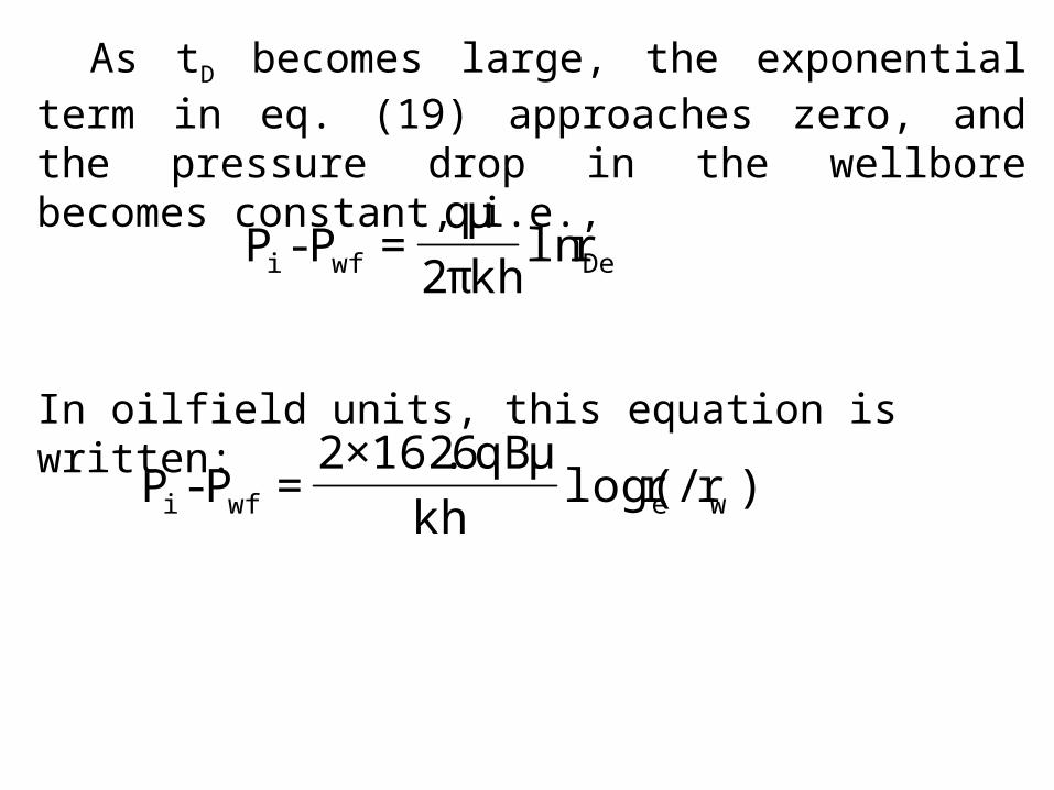
As tD becomes large, the exponential term in eq. (19) approaches zero, and the pressure drop in the wellbore becomes constant, i.e.,
In oilfield units, this equation is written:
Dewfi rlnkh2
qP-P
π
μ=
)r/rlog(kh
qB6.1622P-P wewfi
μ×=
Wellbore Storage and Skin Effect
The following is the equation
(4-7)
where qD = qsf/qqsf = sand face flow rate, cc/sec or STBq = constant surface rate, cc/sec or STBPwD = dimensionless pressure drop in the wellbore
(Darcy units)
∫Dt
0 D
DDDwD d
dt
)-t(dP)(qP τ
ττ=
μ
π=
q
)P-P(kh2 wfi
(oilfield units)
CD = dimensionless wellbore storage coefficient PD = dimensionless constant terminal rate solution to the radial flow equation
Eq. (4-7) is an integro-differential equation. Its solution is easily obtained by Laplace transform method. Thus the Laplace transform of eq. (4-7) is obtained as follows:
μ=
qB2.141
)P-P(kh wfi
]d
)(dPC-1[)(q wD
DD τ
τ=τ
L[PwD] = PwD (z) L[PD] = PD (z)
L[qD(τ)] = (1/z) - zCDPwD(z)
L[dPD/dtD] = z PD (z), since PD = 0 at tD = 0
Thus, in the Laplace domain, eq. (4-7) is written:
PwD(z) = [1 – z CD PwD (z)]PD (z) or
(11-46))]z(PCz1[
)z(P)z(P
DD2
DwD +
=
For tD values usually encountered in well testing, the solution of the radial flow equation (eq.(1)) is familiar Ei function solution. The Ei function solution is expressed by:
By eq. (11-12), the Laplace transform of PD is given by:
From a table of Laplace transforms, the Laplace transform of the function on the right hand side of the previous equation is equal to K0 (√z).
DD
t
0D
/1-
D t4,dtt
e
2
1P ∫
D
=α=α
[ ] ]t
e
2
1[L
z
1PL
D
/1-
D
α
×=
Thus,
L(PD) = K0(√z)/z
Substituting in eq. (11-46), we obtain:
(11-47)
Upon inversion, eq. (11-47) yield the following result:
(11-48)
)]z(KzC1[z
)z(K)z(P
0D
0wD +
=
∫∞
0 20D
220D
2
0tu-
D du])}u(J
2Cu{)}u(Y
2Cu1[{u
)u(J)e-1(P
D2
π+
π+
=
We know that PD is the solution to the radial flow equation which is valid at any rD. Without the skin, PD is valid even at rD = 1, i.e., at the wellbore. Thus, without the skin,
But, in the presence of a skin zone of infinitesimal thickness surrounding the wellbore,
we defined ∆Pskin in oilfield units as:
1DrDwD PP
==
skinDDwD )P(PP1Dr
Δ+==
psi,Skh
qB2.141Pskin
μ=Δ
In Darcy units, the above definition takes the following form:
From these definitions, the dimensionless ∆Pskin, (∆PD)skin, is given by:
(oilfield units) = S (Darcy units)
= S
atm,Skh2
qPskin π
μ=Δ
skinskinD PqB2.141
kh)P( Δ×
μ=Δ
skinskinD Pq
kh2)P( Δ×
μ
π=Δ
In the presence of wellbore storage, ∆Pskin must be given in terms of qsf. Thus, in Darcy units,
or,
(11-49) = qD (tD)S
Skh2
qP sf
skin π
μ=Δ
Sq
q
kh2
q sf×π
μ=
Sq
q)P( sf
skinD =Δ
( ) S]dt
)t(dPC-1[P
D
DwDDskinD =Δ
Therefore, we incorporate the skin by simply adding eq. (11-49) to eq. (4-7). The result is:
(11-50)
From eq. (11-49),
By eq. (11-46), we get:
S]dt
)t(dPC-1[
ddt
)-t(dP]
d
)(dPC-1[P
D
DwDD
D
DD
t
0
wDDwD ∫
D
+
ττ
τ
τ=
[ ] )z(PzSC-)z/S(S)t(qL wDDDD =
[ ])]z(PCz1[
)z(PzSC-
z
SS)t(qL
DD2
DDDD +
=)]z(PCz1[z
S
DD2+
=
The Laplace transform of eq. (11-50) is obtained by adding the Laplace transform of eq. (11-49) to eq. (11-46).
Thus,
We have established that by assuming the Ei function solution to the radial flow equation, L[PD] = K0 (√z)/z. Thus, by substituting in the above equation we obtain:
)]z(PCz1[z
S
)]z(PCz1[
)z(P)z(P
DD2
DD2
DwD +
++
=
)]z(PCz1[z
S)z(zP
DD2
D
+
+=
)]z(KzC1[z
S)z(K)z(P
0D
0wD +
+= (11-51)
As pointed out by Agarwal et al. (1970), because the above equation is based on the Ei function solution of eq. (1), it is only valid after a few seconds from the instant of producing the well at the constant rate, q.
van Everdingen (1953) presented the inverse Laplace transform of eq. (11-51) as follows:
(11-52)
∫∞
0 20
2D
20D
2D
2
0tu-
wD
})]u(JuC21
[)]u(YCu21
SCu-1{[u
du)u(J)e-1(P
D2
π+π+=
van Everdingen pointed out that after a long time, eq. (11-52) reduced to:
which is equivalent to eq. (1-22). Note also that with S = 0, eq. (11-52) reduces to eq. (11-48).
[ ] S80908.0tln2
1P DwD ++=
A more general solution to the problem of wellbore storage and skin was presented by Ramey and Agarwal (1972) who stated the boundary value problem as follows:
(11-5)
subject to the following initial and boundary conditions:
1.
2.
3.
D
D
D
D
D2D
D2
t
P
r
P
r
1
r
P
∂
∂=
∂
∂×+
∂
∂
0)0,r(P DD =
0)t,r(Plim DDD∞→rD
=
1]r∂
P∂r-[
dt
dPC 1r
D
DD
D
wDD D
=+ =
1rD
DDDwD D
}]r∂
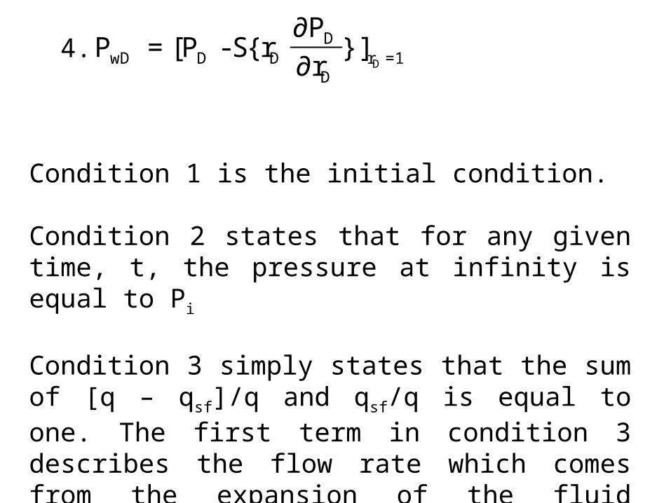
P∂r{S-P[P == 4.
Condition 1 is the initial condition.
Condition 2 states that for any given time, t, the pressure at infinity is equal to Pi
Condition 3 simply states that the sum of [q – qsf]/q and qsf/q is equal to one. The first term in condition 3 describes the flow rate which comes from the expansion of the fluid contained in the wellbore.
In the Laplace domain, the boundary value problem is stated:
1.
2.
3.
4.
The solution is given by eq. (9). However, by applying condition 2, we conclude that A must be zero, and
)z(zPdr
)z(dP
r
1
dr
)z(PdD
D
D
D2D
D2
=+
0)0,r(P DD =
0)z,r(Plim DD∞→rD
=
z
1]
rd
)z(Pdr-[)z(PzC 1r
D
DDwDD D
=+ =
1rD
DDDwD D
}]rd
)z(Pdr{S-(z)P[)z(P ==
the solution is given by eq. (11-39). Thus,
(11-39)
Applying condition 3, we get:
From which,
Thus,
)zr(BK)z(P D0D =
)zr(KzB-dr
)z(dPD1
D
D =
z
1)]zr(KzB-(r[-)z(PzC 1rD1DwDD D
==
)z(Kz
)z(PCz-1B
12/3
wDD2
=
)z(Kz
)zr(K)]z(PCz-1[)z(P
12/3
D0wDD2
D =
Substituting the above in condition 4, we get
Solving this expression for PwD (z), we get:
(11-53)
Agarwal et al. (1970) reported that the heat flow analog of eq. (11-53) was inverted. They presented the time domain equivalent of this equation as follows:
[ ])z(KzS)z(Kz
)]z(PCz-1[)z(P 102/3
wDD2
wD +×=
)]z(KzS)z(K[Cz)z(Kz
)z(KzS)z(K)z(P
10D2
12/3
10wD ++
+=
∫∞
0 21
2D0D
21D
20D
30
tu-
2DDwD })]u(Y)SuC-1(-)u(YuC[)]u(J)SCu-1(-)u(JuC{[u
du)u(J)e-1(4)t,C,S(P
D2
+π=
Ramey and Agarwal (1972) also presented a solution for the case of varying CD.
This situation occurs when the well is initially closed and both casing-head and tubing-head pressures are equal, and upon producing the well the casing-head pressure drops due to the unloading into the tubing of the fluid contained in the annulus.
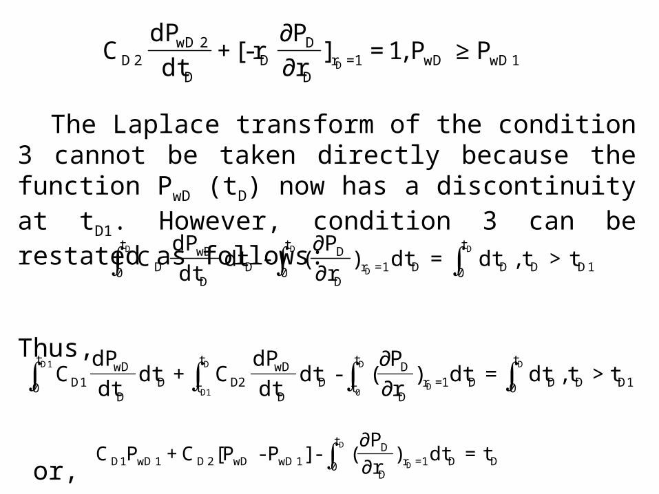
For this case, the boundary value problem is stated exactly as before with the exception of condition 3, which is now stated as:
wD1wD1rD
DD
D
1wD1D P≤P≤0,1]
r∂
P∂r-[
dt
dPC
D=+ =
1wDwD1rD
DD
D
2wD2D PP ,1]
r∂
P∂r-[
dt
dPC
D≥=+ =
The Laplace transform of the condition 3 cannot be taken directly because the function PwD (tD) now has a discontinuity at tD1. However, condition 3 can be restated as follows:
Thus,
or,
∫ ∫ ∫D D D
D
t
0
t
0
t
0 1DDDD1rD
DD
D
wDD tt,dtdt)
r∂
P∂(-dt
dt
dPC >==
∫ ∫ ∫∫1D D
0
D
D
D
D1
t
0
t
t
t
0 1DDDD1rD
Dt
t DD
wDD2D
D
wD1D tt,dtdt)
r∂
P∂(-dt
dt
dPCdt
dt
dPC >=+ =
∫D
D
t
0 DD1rD
D1wDwD2D1wD1D tdt)
r∂
P∂(-]P-P[CPC =+ =
Since PwD1 is a constant, the Laplace transform of condition 3 is:
With this condition 3, the constant B is given by:
Accordingly,
( )21r
D
DwD2D2D1D1wD z
1}
dr
)z(dP{
z
1-)z(PCC-CP
z
1D
=+ =
)z(Kz
)C-C(P-)z(zPC-z/1B
1
2D1D1wDwD2D=
})]z(KzS)z(K[SC)z(Kz
)z(KzS)z(K){C-C(P-
})]z(KzS)z(K[SC)z(Kz
)z(KzS)z(K{
z
1)z(P
102D1
102D1D1wD
102D1
10wD
++
+
++
+=
Hydraulically Fractured Wells for Infinite Conductivity Vertical Fracture
Infinite conductivity fractures are usually much shorter than finite conductivity fractures, and therefore the assumption of infinite conductivity is often justified
By assigning infinite conductivity to the fracture, the effective shape of the well changes from the usual cylindrical shape to the tabular shape of the fracture.
The boundary value problem associated with infinite conductivity fractures is much more involved than the problem of finite conductivity fracture.
Its formulation was given by Russell and Truitt (1964) as a numerical solution. The analytical solution was given by Gringarten et al. (1974) on the basis of Green’s and source functions that were presented by Gringarten and Ramey (1973).
We will not present Gringarten’s solution here because it relies on Green’s source functions, which require a good knowledge of potential theory
Also, for well test interpretation, the complete solution is not needed. What is needed is the early time solution, which followed by transitional period and then by the pseudo-radial period.
The formulation of the early time solution is rather simple. We will assume that during early time the flow from the reservoir into the fracture is linear and perpendicular to the fracture.
We let the fracture coincide with the x-axis. Thus, during early time, the flow would be parallel to the y-axis and in opposite sense with respect to the fracture.
The boundary value problem is stated, in Darcy units, as follows:
)t,y(P-PP,t∂
P∂
k
c
y∂
P∂i
t2
2
=ΔΔ
×φμ
=Δ
0)0,y(P =Δ
0)t,y(Plim∞→y
=Δ
k)hx4(
q-
y∂
P∂
f0y
μ=
Δ
=
1.
2.
3.
Condition 1 is the usual initial condition. Condition 2 implies that we are assuming an infinite reservoir. Condition 3 implies that the flow into the fracture follows Darcy’s law with the area of the fracture equal to a xfh.
With definitions given previously for PD, tDxf, and yD we can state the boundary value problem in dimensionless form as follows:
(11-125)
1.
2.
3.
Dxf
D2D
D2
t
P
y
P
∂
∂=
∂
∂
0)0,y(P DD =
0)t,y(Plim DxfDD∞→yD
=
2-
y∂
P∂
0yD
D
D
π=
=
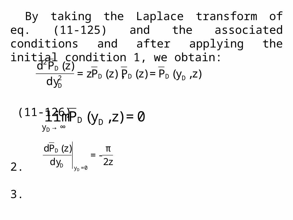
By taking the Laplace transform of eq. (11-125) and the associated conditions and after applying the initial condition 1, we obtain:
(11-126)
2.
3.
The general solution of eq. (11-126) is given by:
)z,y(P)z(P),z(Pzdy
)z(PdDDDD2
D
D2
==
0)z,y(Plim DD∞→yD
=
z2-
dy
)z(Pd
0yD
D
D
π=
=
zyzy-DD
DD BeAe)z,y(P ++= (11-127)
By condition 2 the constant B in eq. (11-126) must be set to zero. By applying condition 3, we get;
and,
zy-
D
DDDezA-
dy
)z,y(Pd=
z2-zA-
dy
)z,y(Pd
0yD
DD
D
π==
=
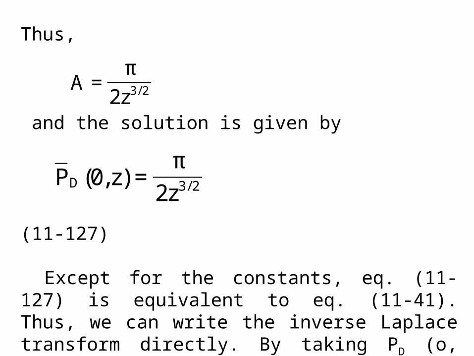
Thus,
and the solution is given by
(11-127)
Except for the constants, eq. (11-127) is equivalent to eq. (11-41). Thus, we can write the inverse Laplace transform directly. By taking PD (o, tDxf) = PwD, the solution in the time domain is given by
2/3z2A
π=
2/3Dz2
)z,0(Pπ
=
DxfwD tP π= (11-128)
In oilfield units, the solution takes the following forms:
For oil:
(11-129)
For gas:
(11-130)
2/12/1
tf
00wfi t]
ck[
hx
Bq064.4P-P
φ
μ=
2/12/1
tgf
g
wfi t]ck
1[
hx
Tq985.40)P(m-)P(m
φμ=
Testing of Hydraulically Fractured Wells for Finite Conductivity Vertical Fracture
Here we will present the theoretical background for the case of the finite conductivity, vertically fractured wells. WE will follow to some extent the presentation given by Cinco-Ley et al. (1978) and Cinco-Ley (1981).
Fig. 11-1 shows a vertical fracture of width w and length 2xf which is symmetrically centered with respected to the wellbore. Fig. 11-2 shows a plan view of the fracture, the position of the x-axis and the stipulated linear flow pattern inside the fracture.
Fig. 11-3 shows the stipulated changes in the flow pattern with respect to time.
At early time the flow comes only from the expansion of the fluid contained in the fracture (Fig. 11-3a).
After a transition period, a bilinear flow period develops (Fig. 11-3b). This is sometimes followed by a formation linear flow period (Fig. 11-3c)
Finally the system reaches the pseudo-radial flow period as shown in Fig. 11-3d.
Now we want to solve eq. (11-108) subject to the following initial and boundary conditions:
1. ∆Pf (x, t=0) = 0 for 0 ≤ x ≤ xf
2.
3.
Condition 1 is the usual initial condition. It states that initially Pf (x, t=0) = Pi. Condition 2 states that the rate produced from the well, qw, is given by:
0t,hwk2
q-
x∂
P∂
f
w
0x
f >μ
=Δ
=
0t,0x∂
P∂
fxx
f >=Δ
=
0x
ffw x∂
P∂Ak-q
=
Δ×
μ=
where A = area of the well. The well is assumed to be a vertical plane as shown in Fig. 11-2.
Thus, A = w h, cm
Condition 3 states that no fluid enters the fracture at its tips.
Eq. (11-108) describes the flow in the fracture. We need another equation that describes the linear flow in the reservoir. This equation and the initial & boundary conditions are given as follows
t∂
P∂
k
c
y∂
P∂ t2
2 Δ×
φμ=
Δ (11-109)
1. ∆(x, y, t=0) = 00, 0 < y <∞
2.
3.
Before attempting to solve eqs. 911-108) & (11-109), it is best to transfer these equations and boundary conditions to their dimensionless forms.
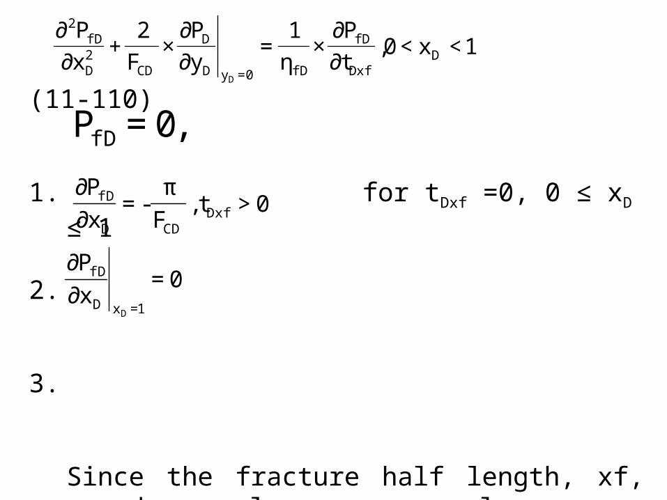
In dimensionless form eq. (11-108) and the initial and boundary conditions are given by:
μ
π=
q
))t,y,x(P-P(kh2P fi
fD
2ft
Dxf xc
ktt
φμ=
tff
tf
ck
ckfD φ
φ=η
1x0,t∂
P∂1
y∂
P∂
F
2
x∂
P∂D
Dxf
fD
fD0yD
D
CD2D
fD2
D
<<×η
=×+=
(11-110)
1. for tDxf =0, 0 ≤ xD ≤ 1
2.
3.
Since the fracture half length, xf, can be as large as we please, eq. (11-110) can be made valid for 0 < xD <∞ by changing condition 3. Thus,
,0PfD =
0t,F
-x∂
P∂Dxf
CDD
fD >π
=
0x
P
1xD
fD
D
=∂
∂
=
∞≤x≤0,t
P∂1
y∂
P∂
F
2
x∂
P∂D
Dxf
fD
fD0yD
D
CD2D
fD2
D
×η
=×+=
(11-111)
1.
2.
3.
In dimensionless form, eq. (11-109) and its initial and boundary conditions are given by:
,0PfD = for tDxf =0, 0 ≤ xD <∞
0t,F
-x∂
P∂Dxf
CDD
D >π
=
0t,0Plim DxffD∞→xD
>=
∞y0,t∂
P∂1
y∂
P∂D
Dxf
D
fD2D
D2
<<×η
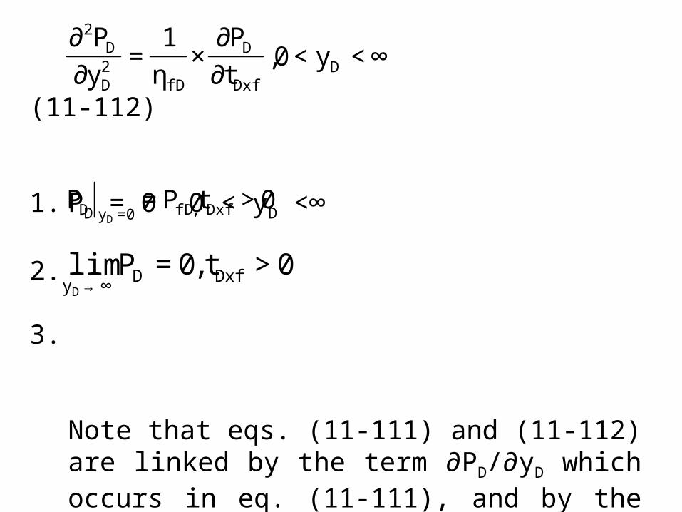
= (11-112)
1. PD = 0 0 < yD <∞
2.
3.
Note that eqs. (11-111) and (11-112) are linked by the term ∂PD/∂yD which occurs in eq. (11-111), and by the boundary conditions.
0tPP Dxf,fD0yDD
>==
0t,0Plim DxfDyD
>=∞→
To solve eqs. (11-111) and (11-112), we take the Laplace transform with respect to tDxf and apply the initial condition 1. Thus,
(11-113)
2.
3.
and
(11-114)
)z(Pz
dy
)z(dP
F
2
dx
)z(PdfD
fD0yD
D
CD2D
fD2
D
η=×+
=
CD0xD
fD
zF-
dx
)z(dP
D
π=
=
0)z(Plim fD→xD
=
)z(zPdy
)z(PdD2
D
D2
=
)z(P)z(P fD0yDD
==
2.
3.
Note that, PD (z) = PD (xD, yD, z)
To solve eq. (11-114), we take the Laplace transform once more, but this time we take it with respect to yD. For this purpose we will use the Laplace parameter, r, and the transform expression of the second derivative. In terms of the Laplace parameter r, this expression is written as follows:
0)z(Plim D∞→yD
=
[ ] )0(F-)0(rf-)r(fr)t(FL '2'' =
Thus, the Laplace transform of eq. (11-114) is given by:
By condition 2, PD(0,z) = PfD(z), we obtain:
(11-115)
)z,r(zPdy
)z,0(dP-)z,0(rP-)z,r(Pr D
D
DDD
2 =
z-r
dy)z,0(dP
)z(rP
)z,r(P 2D
DfD
D
+
=
The inversion of eq. (11-115) with respect to the Laplace parameter, r, is found by referring to a table of transforms and is given by:
(11-116)
where cosh (u) =hyperbolic cosine of u = ½(eu – e-u)
sinh (u) = hyperbolic sine of u = ½(eu + e-u)
By applying condition 3, , to eq. (11-116)
z
)yzsinh(
dy
)z(dP)yzcosh()z(P)z(P D
0yD
DDfDD
D
×+==
1)e-e/()ee(lim)utanh(lim u-uu-u
∞→u∞→u=+=
0)z(Plim D→yD
=∞
we get:
(11-117)
Substituting eq. (11-117) in eq. (11-113) we obtain
an equation with one dependent variable. Thus,
(11-118)
By applying the conditions associated with eq. (11-113) to above equation, we obtain:
(11-119)
)z(Pz-dy
)z(dPfD
0yD
D
D
==
)z(PF
z2z
dx
)z(PdfD
CDfD2D
fD2
+η
=
2/1
CDfDCD
2/1
CDfDD
fD
]F
z2z[zF
}]F
z2z[x-exp{
)z(P
+η
+η
π
=
At the wellbore, xD = 0 and PfD(z) = PwD (z). Thus, substituting xD = 0 in eq. (11-119), we obtain
(11-120)
Eq. (11-120) can be written as follows:
(11-120a)
and,
(11-120b)
2/1
CDfDCD
wD
]F
z2z[zF
)z(P
+η
π=
2/1
CDfD
2/3CD
wD
]Fz
21[zF
)z(P+
η
π=
2/1
CD
2/5
fD
3
CD
wD
]Fz2z
[F)z(P
+η
π=
At early time, z is very large and the second term in the denominator of eq. (11-120a) is negligible.
On the other hand, at later time z is very small and the first term in the denominator of eq. (11-120b) is negligible. Thus, we can write:
For early time:
(11-121)
For later time:
(11-122)
zF≈)z(P 2/3
CD
fDwD
ηπ
zF2≈)z(P 4/5
CDwD
π
Eqs. (11-121) and (11-122) can be inverted by referring to a table of Laplace transforms. Thus,
For early time:
(11-123)
For later time:
(11-124)
Eq. (11-123) shows that a plot of PwD vs. tDxf on log-log graph paper would be a straight line of slope of one half.
DxffDCD
wD tF
2P πη=
4/1Dxf2/1
CDwD )t(
)F(
45.2P =
Eq. (11-124) shows that the same plot would produce a straight line of slope one quarter.
To obtain equations equivalent to equations (11-123) and (11-124) in oilfield units, we substitute for tDxf and PwD as follows: