Radar Imaging: An Introduction

Kaitlyn MullerGraduate Workshop on Inverse Problems

Colorado State University

August 10, 2016

1

What is radar?

Did you know radar is an acronym?

RADAR = RAdio Detection And Ranging

Radar originally was developed for echolocation

Radar now can be used for more complicated tasks, i.e. imaging

2

What is radar?

Did you know radar is an acronym?

RADAR = RAdio Detection And Ranging

Radar originally was developed for echolocation

Radar now can be used for more complicated tasks, i.e. imaging

2

What is radar?

Did you know radar is an acronym?

RADAR = RAdio Detection And Ranging

Radar originally was developed for echolocation

Radar now can be used for more complicated tasks, i.e. imaging

2

What is radar?

Did you know radar is an acronym?

RADAR = RAdio Detection And Ranging

Radar originally was developed for echolocation

Radar now can be used for more complicated tasks, i.e. imaging

2

Why use radar?

can be used day or night

measures target range accurately and can also measure the rateat which range is changing (i.e. can measure velocity)

waves pass through clouds, smoke, etc. (i.e. its an all weathersensor)

can penetrate foliage, buildings, sand, etc.

waves scatter from objects and features that are of the same sizeorder as the transmitting wavelength ⇒ radar is sensitive toobjects whose length scales range from cm to m

3

Why use radar?

can be used day or night

measures target range accurately and can also measure the rateat which range is changing (i.e. can measure velocity)

waves pass through clouds, smoke, etc. (i.e. its an all weathersensor)

can penetrate foliage, buildings, sand, etc.

waves scatter from objects and features that are of the same sizeorder as the transmitting wavelength ⇒ radar is sensitive toobjects whose length scales range from cm to m

3

Why use radar?

can be used day or night

measures target range accurately and can also measure the rateat which range is changing (i.e. can measure velocity)

waves pass through clouds, smoke, etc. (i.e. its an all weathersensor)

can penetrate foliage, buildings, sand, etc.

waves scatter from objects and features that are of the same sizeorder as the transmitting wavelength ⇒ radar is sensitive toobjects whose length scales range from cm to m

3

Why use radar?

can be used day or night

measures target range accurately and can also measure the rateat which range is changing (i.e. can measure velocity)

waves pass through clouds, smoke, etc. (i.e. its an all weathersensor)

can penetrate foliage, buildings, sand, etc.

waves scatter from objects and features that are of the same sizeorder as the transmitting wavelength ⇒ radar is sensitive toobjects whose length scales range from cm to m

3

Why use radar?

can be used day or night

measures target range accurately and can also measure the rateat which range is changing (i.e. can measure velocity)

waves pass through clouds, smoke, etc. (i.e. its an all weathersensor)

can penetrate foliage, buildings, sand, etc.

waves scatter from objects and features that are of the same sizeorder as the transmitting wavelength ⇒ radar is sensitive toobjects whose length scales range from cm to m

3

Radar Imaging Tasks

Transmitting microwave energy at high power - engineering task

Detecting microwave energy - engineering/math task

Interpreting and extracting information from received signals -where the math comes in

4

Math for Radar

PDEs (electromagnetic theory, wave propagation)

harmonic analysis, group theory, microlocal analysis

linear algebra, sampling theory

statistics

scientific computing

coding theory, information theory

5

Radar history

1886 Heinrich Hertz confirmed radio wave propagation

1904 Hulsmeyer patented ship collision avoidance system

1922 ship detection methods at NRL (Taylor & Young)

1930 Hyland used radar to detect aircraft (led to first US radarresearch effort directed by NRL)

1930s England and Germany radar programs developed (ChainHome early warning system, fire control systems, aircraftnavigation systems, cavity magnetron to transmit high-powermicrowaves)

1940s establishment of MIT Rad Lab (radar for tracking, U-boatdetection)

6

Radar Images

7

Radar Images

8

Radar Images

9

Imaging Methods - Detection and rangingIn the first image we saw an example of echolocation, how is thisperformed?

First transmit an EM wave and measure the reflected field as atime-varying voltage

At time t = 0 a short pulse travels at speed c , this reflects froman object at range R, and returns to the radar

If the pulse is detected at time τ how can we easily calculate thetarget’s range?

Distance = rate * time ⇒ R = cτ/2

10

Imaging Methods - Detection and rangingIn the first image we saw an example of echolocation, how is thisperformed?

First transmit an EM wave and measure the reflected field as atime-varying voltage

At time t = 0 a short pulse travels at speed c , this reflects froman object at range R, and returns to the radar

If the pulse is detected at time τ how can we easily calculate thetarget’s range?

Distance = rate * time ⇒ R = cτ/2

10

Imaging Methods - Detection and rangingIn the first image we saw an example of echolocation, how is thisperformed?

First transmit an EM wave and measure the reflected field as atime-varying voltage

At time t = 0 a short pulse travels at speed c , this reflects froman object at range R, and returns to the radar

If the pulse is detected at time τ how can we easily calculate thetarget’s range?

Distance = rate * time ⇒ R = cτ/2

10

Imaging Methods - Detection and rangingIn the first image we saw an example of echolocation, how is thisperformed?

First transmit an EM wave and measure the reflected field as atime-varying voltage

At time t = 0 a short pulse travels at speed c , this reflects froman object at range R, and returns to the radar

If the pulse is detected at time τ how can we easily calculate thetarget’s range?

Distance = rate * time ⇒ R = cτ/2

10

Imaging Methods - Detection and rangingIn the first image we saw an example of echolocation, how is thisperformed?

First transmit an EM wave and measure the reflected field as atime-varying voltage

At time t = 0 a short pulse travels at speed c , this reflects froman object at range R, and returns to the radar

If the pulse is detected at time τ how can we easily calculate thetarget’s range?

Distance = rate * time ⇒ R = cτ/2

10

High-range resolution imagingIn echolocation there is an assumption that we model eachtarget as a single pointMost objects are more complicated, so we consider them acollection of points or scattering centersThe received response at the radar will be a superposition ofreflections from single points

11

Real-Aperture imaging

uses fixed antenna with a narrow beam

scan beam over region of interest

at each scan location and pulse delay the system plots receivedintensity

12

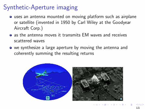
Synthetic-Aperture imaginguses an antenna mounted on moving platform such as airplaneor satellite (invented in 1950 by Carl Wiley at the GoodyearAircraft Corp.)

as the antenna moves it transmits EM waves and receivesscattered waves

we synthesize a large aperture by moving the antenna andcoherently summing the resulting returns

13

Equations of Electromagnetic Wave Propagation

Electromagnetic waves are governed by Maxwell’s equations (in timedomain)

∇× E(x , t) = −∂B(x , t)

∂t

∇×H(x , t) = J (x , t) +∂D(x , t)

∂t∇ · D(x , t) = ρ(x , t)

∇ · B(x , t) = 0

where E is the electric field, B is the magnetic induction field, D isthe electric displacement field, H is the magnetic intensity/field, ρ isthe charge density, and J is the current density.

14

Equations of EM Wave propagation continued

Most radar propagation takes place in dry air which is wellmodeled by free space

Therefore we make further assumptions:

ρ(x , t) = 0

J (x , t) = 0

We also have the free space constitutive relations

D = ε0E B = µ0H

where ε0 is the electric permittivity in free space and µ0 is themagnetic permeability in free space.

15

Working towards the wave equationTaking the curl of the first of Maxwell’s equations and then inserting theconstitutive relation we have

∇× (∇× E) = ∇×(− ∂B(x , t)

∂t

)= −µ0

∂

∂t(∇×H)

Now using the 2nd Maxwell equation, the fact that J = 0, and the otherconstitutive relation we obtain

∇× (∇× E) = −µ0ε0∂2E∂t2

Finally we use the triple-product identity to rewrite the left-hand side

∇× (∇× E) = ∇(∇ · E)−∇2E = −µ0ε0∂2E∂t2

We note that since ρ = 0⇒ ∇ · D = 0⇒ ∇ · E = 0 and therefore weobtain the wave equation

∇2E = µ0ε0∂2E∂t2

16

Propogation in frequency domain

We define the Fourier transform of E to be

E (x , ω) =

∫e iωtE(x , t)dt

Now taking the FT of the wave equation we obtain theHelmholtz equation

∇2E + k2E = 0

where k = ω/c is the wave number, c = 1/√µ0ε0 is the speed

of light in free space, ω is angular frequency, and λ = 2πc/ω isthe wavelength

17

Note on boundary conditions

Uniqueness of solutions of Helmholtz equation requires thesolutions to obey the B.C.s of a wave radiating outward from asource.

These B.C.s require that solutions decay to 0 at a rate 1/R asR →∞ and that they are outgoing, i.e.

E (x , ω) = O(R−1) as R →∞∂E∂r− ikE = o(R−1) as R →∞

where R = |x | and the second condition is widely known as theSommerfeld radiation condition.

18

Introduction to scattering in 1D

Consider an antenna at x = 0 and an infinite (PEC) plate at x = R

Assume waveform generator produces a waveform s which is multiplied by acarrier wave (upmodulation) to produce the signal

f (t) = s(t) cos(ω0t)

where ω0 is the carrier frequency.

We take the incident field to be

E in(x , t) = E inf (t − x/c)

Note E tot = E in + E sc where the total field must satisfy the wave equationand B.C.s.

E tottan

∣∣∣∣x=R

= 0 ⇔ E sc

∣∣∣∣x=R

= −E in

∣∣∣∣x=R

19

1D scattering continued

This leads us to expect that the scattered field is left-traveling and of theform

E sc(x , t) = E scg(t + x/c)

Using the B.C. with our assumption ⇒

E scg(t + R/c) = −E inf (t − R/c)

We obtain the final solution by choosing E sc = −E in and we letg(u) = f (u − 2R/c) where u = t + R/c and t = u − R/c

E sc(x , t) = −E inf (t + x/c − 2R/c)

Evaluating at x = 0 where the antenna is location we find our receivedsignal

E sc(x = 0, t) = −E inf (t − 2R/c)

20

Moving PEC plate

Assume the position of the plate is moving, i.e. x = R(t) = R + vt

We still have that

E scg(t + R(t)/c) = −E inf (t − R(t)/c)

Now using the same substitute u = t + R(t)/c ⇒ t = u−R/C1+v/c we obtain

g(u) = f (α(u − R/c)− R/c)

where α = 1−v/c1+v/c = 1− 2v/c + O((v/c)2) is called the Doppler scale factor

Therefore the scattered field at x = 0 is

E sc(x = 0, t) = −E inf (α(t − R/c)− R/c)

≈ −E ins(t − 2R/c) cos(ω0[(1− 2v/c)(t − R/c)− R/c])

Note in this case the carrier frequency is shifted by ωD = −2(v/c)ω0

21

Detection of signals in noise

Note we have found the signal received at the radar is a timedelayed (Doppler shifted) version of the transmitted signal.

To get a good estimate of the target range we want to use ashort pulse but this has little energy and is difficult to detect innoise.

D.O. North found a mathematical solution to this problem in1943 by transmitting long coded pulses along with matchedfiltering.

22

Detection of signals in noise continuedThe signal scattered from a fixed, point-like target is

srec(t) = ρs(t − τ) + n(t)

where s is the transmitted pulse, τ = 2R/c , ρ ∝ 1/R4 is the scatteringstrength, and n is noise.

We seek a filter to apply upon reception that will improve thesignal-to-noise ratio (SNR). We define

η(t) = (h ∗ srec)(t) = ρηs(t) + ηn(t)

where ∗ indicated convolution and h is our reception filter.

Goal: signal output ηs at time τ to be as large as possible relative to thenoise.

Define n(t) to be white noise with E [n(t)n(t ′)] = Nδ(t − t ′)

Define SNR

SNR =|ηs(t)|2

E |ηn(t)|2

23

Maximizing SNR

After simplifying the denominator we have that

SNR =|∫h(τ − t ′)s(t ′ − τ)dt ′|2

N∫|h(t)|2dt

performing a change of variables t = τ − t ′ we have

SNR =|∫h(t)s(−t)dt|2

N∫|h(t)|2dt

≤∫|h(t)|2dt

∫|s(−t)|2dt

N∫|h(t)|2dt

=

∫|s(−t)|2dt

N

Therefore SNR is maximized when we choose h(t) = s(−t), this is calledthe matched filter.

We may write our filtered received signal as

η(t) =

∫s(t ′)srec(t ′ + t)dt ′

which is commonly called the correlation between s and srec.

24

Received signal from a distribution of fixed targets

The signal recieved from a distribution of non-interacting targetsis

srec(t) =

∫ρ(τ ′)s(t − τ ′)dτ ′ + n(t)

Application of the matched filter results in

η(t) =

∫s∗(t ′ − t)srec(t ′)dt ′

=

∫χ(t − τ ′)ρ(τ ′)dτ ′ + noise

where χ is the point-spread function (PSF)

χ(t) =

∫s∗(t ′′ − t)s(t ′′)dt ′′

25

More on SNRNote the correlation process improves SNR at the receiver by concentrating energy of thereceived signal at a single delay time (pulse compression)Phase coding is the process of choosing s(t) such that autocorrelation (or PSF) is asclose as possible to ideal, i.e. delta functionMost common choice of signal is the chirp

p(t) = e i(ωmint+γt2/2)u[0,T ](t)

The autocorrelation of a chirp is

χ(τ) = e−iτγ/2 sinc[(T − |τ |)γτ/2]

when |τ | ≤ T and 0 otherwise.

26

Pulse Compression in Noise

27

Received signal from a single moving target

We consider processing signals scattered from moving targets ⇒we hope to form an image that shows both range and velocity

In the case of a single moving target the received signal is

srec(t) = ρs(t − τ)e−iωD(t−τ) + n(t)

We want to find τ and ωD ⇒ we use a set of matched filters,one for every possible Doppler shift (called ’filter bank’)

η(τ, ν) =

∫hν(t − t ′)srec(t ′)dt ′

It is found that the matched filter in this case is given byhν(t) = s(−t)e−iωD t (ωD = 2πνD)

In order to estimate τ and νD we find the arguments of η whereit takes on its maximum.

28

A distribution of moving targetsIn the case of a distribution of moving targets the received signalis of the form

srec(t) =

∫ ∫ρ(τ ′, ν ′)s(t − τ ′)e2πiν′(t−τ ′)dτ ′dν ′ + n(t)

The filter output is

η(τ, ν) =

∫s∗(t ′ − τ)e−2πiν(τ−t′)srec(t ′)dt ′

=

∫ ∫χ(τ − τ ′, ν − ν ′)e−2πiν′(τ−τ ′)ρ(τ ′, ν ′)dτ ′dν ′ + noise term

where χ is the radar ambiguity function (aka the PSF forrange-doppler imaging)

χ(τ, ν) =

∫s(t ′′ − τ)e−2πiν(τ−t′′)s(t ′′)dt ′′

29

Moving target ‘image’ example

30

The Radar Ambiguity Function

The ambiguity function allows us to analyze the accuracy oftarget range and velocity estimates

Basic Properties (assuming we consider only signals that arenormalized by their total energy):

I |χ(τ, ν)| ≤ 1I∫ ∫|χ(τ, ν)|2dτdν = 1 (conservation of ambiguity volume)

I |χ(−τ,−ν)| = |χ(τ, ν)|I The magnitude of the ambiguity function remains the same

when the signal is translated in timeI Modulation does not change magnitude

Note the conservation of ambiguity volume ⇒ the radaruncertainty principle: a waveform with good range resolution haspoor Doppler resolution

31

Range Resolution

To study range resolution we consider a fixed target, i.e. ν = 0

|χ(τ, 0)| = |∫

s∗(t ′)s(t ′ + τ)dt ′|

= |∫|S(ν)|2e2πiντdν|

where s(t) =∫S(ν)e−2πiντdν.

In order to make |χ| as close as possible to a delta function wewould like |S |2 = 1 but this implies s has infinite energy

We note that the Fourier transform of a narrow peak is broadlysupported in the Fourier domain ⇒ we obtain better rangeresolution when the signal bandwidth is large

32

Doppler Resolution

To study Doppler resolution we consider a target whose range isknown, i.e. τ = 0

|χ(0, ν)| = |∫|s(t)|2e−2πiνtdt|

We obtain better Doppler resolution from a long-duration signal(want |s(t)|2 = 1)

Note this is the opposite of what we want for range resolution

33

Resolution for a ChirpA normalized chirp is

p(t) = e i(ωmint+γt2/2)u[0,T ](t)

The ambiguity function when ν = 0 is found to be

|χ(τ, ν = 0)| = |(T − |τ |) sinc[(T − |τ |)γτ/2]|

We may define resolution as the distance between the peak and the first null of theambiguity function or the distance from null to null

δτpn =2π

Tγ=

4π

B

δτnn =4π

Tγ=

8π

B

where B = 2πTγ is the bandwidth in Hz

For the range we multiply by the speed of the wave giving us the range resolution ofapproximately c/B

For the case τ = 0 we have that |χ(0, ν)| = | sinc(πνT )| ⇒ and the distance from peakto null is 1/T and null to null is 2/T

Using νD = −2vν0/c we obtain the velocity resolution is c/(ν0T ) = λ0/T whereλ0 = c/ν0.

34

Ambiguity function example

35

Conclusions

We may use the scalar wave equation to model EM wavepropagation

Received signals are time-delayed, Doppler shifted versions of thetransmitted signal

Performing a matched filtering process on the received signalgives us maximal signal to noise ratio out of all possible filters

Studying the autocorrelation of signals (i.e. the PSF orambiguity function) tells us the accuracy of range and velocityestimates of targets

36