Annu. Rev.EarthPlanet. Sci. 1995.23:337-74 Copyright (~ 1995 by Annual Reviews Inc. All rights reserved RADAR INVESTIGATION OF MARS, MERCURY, AND TITAN Duane O. Muhlernan Division of Geological and Planetary Sciences, 170-25,California Institute of Technology, Pasadena, California 91125 Arie W. Grossman Laboratory for Millimeter-Wave Astronomy, Department of Astronomy, University of Maryland, College Park, Maryland20742 BryanJ. Butler 1 Division of Geologicaland Planetary Sciences, 170-25, California Institute of Technology, Pasadena, California 91125 KEY WORDS: coherent backscatter, multiple scattering, stealth INTRODUCTION Radarastronomy is the study of the surfaces and near surfaces of Solar System objects using active transmission of modulated radio waves and the detection of the reflected energy. The scientific goals of such experiments are surprisingly broad and include the study of surface slopes, fault lines, craters, mountain ranges, and other morphological structures. Electrical reflectivities contain information about surface densities and; to someextent, the chemical com- position of the surface layers. Radarprobes the subsurface layers to depths of the order of 10 wavelengths, providing geological mapping and determi- nations of the object’s spin state. Radaralso allows one to study an object’s atmosphere and ionic layers as well as those of the interplanetary medium. Pre- cise measurements of the time delay to surface elements provide topographic mapsand powerfulinformation on planetary motions and tests of gravitational theories such as general relativity. In this paper, welimit our discussion to surface and near-surface probing of Mercury,Mars, and Titan and review the I Currently at the National Radio Astronomy Observatory, Socorro, New Mexico. 337 0084-6597/95/0515-0337505.00 www.annualreviews.org/aronline Annual Reviews Annu. Rev. Earth. Planet. Sci. 1995.23:337-374. Downloaded from arjournals.annualreviews.org by CALIFORNIA INSTITUTE OF TECHNOLOGY on 09/13/05. For personal use only.
Transcript
Annu. Rev. Earth Planet. Sci. 1995. 23:337-74Copyright (~ 1995 by Annual Reviews Inc. All rights reserved
RADAR INVESTIGATION OFMARS, MERCURY, AND TITAN
Duane O. Muhlernan
Division of Geological and Planetary Sciences, 170-25, California Institute ofTechnology, Pasadena, California 91125
Arie W. Grossman
Laboratory for Millimeter-Wave Astronomy, Department of Astronomy,University of Maryland, College Park, Maryland 20742
Bryan J. Butler1
Division of Geological and Planetary Sciences, 170-25, California Institute ofTechnology, Pasadena, California 91125
Radar astronomy is the study of the surfaces and near surfaces of Solar Systemobjects using active transmission of modulated radio waves and the detection ofthe reflected energy. The scientific goals of such experiments are surprisinglybroad and include the study of surface slopes, fault lines, craters, mountainranges, and other morphological structures. Electrical reflectivities containinformation about surface densities and; to some extent, the chemical com-position of the surface layers. Radar probes the subsurface layers to depthsof the order of 10 wavelengths, providing geological mapping and determi-nations of the object’s spin state. Radar also allows one to study an object’satmosphere and ionic layers as well as those of the interplanetary medium. Pre-cise measurements of the time delay to surface elements provide topographicmaps and powerful information on planetary motions and tests of gravitationaltheories such as general relativity. In this paper, we limit our discussion tosurface and near-surface probing of Mercury, Mars, and Titan and review the
I Currently at the National Radio Astronomy Observatory, Socorro, New Mexico.
work of the past decade, which includes fundamentally new techniques forEarth-based imaging.
The most primitive experiments involve just the measurement of the to-tal echo power from the object. The most sophisticated experiments wouldproduce spatially resolved maps of the reflected power in all four Stokes’ pa-rameters. Historically, the first experiments produced echoes from the Moonduring the period shortly after World War II (see e.g. Evans 1962), but the sub-ject did not really develop until the early 1960s when the radio equipment wassufficiently sensitive to detect echoes from Venus and obtain the first Dopplerstrip "maps" of that planet. The first successful planetary radar systems werethe Continuous Wave (CW) radar at the Goldstone facility of the Caltech’s JetPropulsion Laboratory and the pulse radar at the MIT Lincoln Laboratory. Allof the terrestrial planets were successfully studied during the following decade,yielding the spin states of Venus and Mercury, a precise value of the astronom-ical unit, and a host of totally new discoveries concerning the surfaces of theterrestrial planets and the Moon. This work opened up at least a similar numberof new questions. Although the early work was done at resolution scales onthe order of the planetary radii, very rapid increases in system sensitivities im-proved the resolution to the order of 100 km, but always with map ambiguities.Recently, unambiguous resolution of 100 m over nearly the entire surface ofVenus has been achieved from the Magellan spacecraft using a side-looking,synthetic aperture radar. Reviews of the work up to the Magellan era can befound in Evans (1962), Muhleman et al (1965), Evans & Hagfors (1968, chapters written by G Pettengill, T Hagfors, and J Evans), and Ostro (1993).The radar study of Venus from the Magellan spacecraft was a tour de force andis well described in special issues of Science (volume 252, April 12, 1991) andin the Journal of Geophysical Research (volume 97, August 25 and October25, 1992). Venus will not be considered in this paper even though importantpolarization work on that planet continues at Arecibo, Goldstone, and the VeryLarge Array (VLA).
In this paper we review the most recent work in Earth-based radar astronomyusing new techniques of Earth rotation, super synthesis at the VLA in NewMexico (operated by the National Radio Astronomy Observatory), and the re-cently developed "long-code" techniques at the Arecibo Observatory in PuertoRico (operated by Cornell University). [Note: It was recently brought to ourattention that the VLA software "doubles" the flux density of their primary cal-ibrators. Consequently, it is necessary to half the radar power and reflectivitynumerical values in all of our published radar results from the VLA/Goldstoneradar.] The symbiotic relationship in these new developments for recent ad-vances in our understanding of Mercury and Mars is remarkable. VLA imagingprovides for the first time, unambiguous images of an entire hemisphere of aplanet and the long-code technique makes it possible to map Mars and Mercury
using the traditional range-gated Doppler strip mapping procedure [which was,apparently, developed theoretically at the Lincoln Laboratory by Paul Green,based on a citation in Evans (1962)]. Richard Goldstein was the first to ob-tain range-gated planetary maps of Venus as reported in Carpenter & Goldstein(1963). Such a system was developed earlier for the Moon as reported Pettengill (1960) and Pettengill & Henry (1962)). We first discuss the synthesis mapping technique.
The use of the VLA as the radar receiving instrument allows one to make aspatial map of the echo power with a resolution only limited by the resolvingpower of the VLA. The ultimate resolution at the radar wavelength of 3.5 cmis 0.2 arc sec, achieved when the VLA is in its largest configuration with amaximum spacing between antenna elements of 36 km. This resolution cor-responds to 145 km at a distance of 1 astronomical unit (AU). These valuesare actually the minimum fringe spacing for the instrument (at 3.5 cm), andthe image resolution achieved in real maps is degraded by about 50%. Thesenew techniques allowed observers at the VLA to obtain complete, unambigu-ous radar maps of the Earth-facing hemispheres of the terrestrial planets. TheVLA/Goldstone radar has a bistatic configuration with the NASA/JPL 70-mantenna at Goldstone transmitting at a wavelength of 3.5 cm and with radiatedpower up to 460,000 watts in the monochromatic or CW mode. The exacttransmitter frequency is tuned with a programmed local oscillator, which re-moves the Doppler shift caused by the the motion of the center of mass of thetarget planet with respect to the transmitter and the receiver system at the VLA.Thus, the reflected radar energy is received with the VLA 27-antenna inter-ferometer as though the reflected flux density was "emitted" from a celestial,narrow-band spectral line source. The CW transmitted signal is Doppler-spreadat reflection due to the relative rotational motion of each reflecting point on theplanet. In principle, it is possible to take advantage of the Doppler strip res-olution in the VLA mapping to greatly increase the spatial resolution in "onedimension." However, the available minimum frequency resolution at the VLAis insufficient to resolve in frequency planetary objects other than Mars andSaturn’s rings. The maximum spectral width for the targets of interest areabout 200, 400, 1340, and 28,000 Hz for Venus, Mercury, Titan, and Mars,respectively. Unfortunately, the minimum frequency resolution at the VLA is381 Hz if just a single polarization is to be recorded; that value must be doubledif two polarized signals are to be recorded. The VLA/Goldstone radar utilizesa circularly polarized transmitted signal [usually Right Circular Polarization(RCP)] and it is desirable to receive the echo energy in both RCP and LeftCircular Polarization (LCP), which dictates a minimum frequency resolutionof 763 Hz. Thus, in the cases of Venus and Mercury, all of the echo energyis in a single spectral channel that is wider than the signal spectrum, caus-ing a loss in sensitivity. If all four Stokes’ parameters were to be measured,
another doubling of the minimum bandwidth to 1526 Hz would be required.Only then could the response in both the circular and two linear modes ofpolarization be derived from the amplitudes and phases measured in circularpolarization.
The study of the physical properties of a planetary surface is greatly aidedby measuring the polarization properties in the echoes. Quite generally, thestrongest reflections from a natural surface will be obtained for circularly po-larized transmitted signals by measuring the echo in the circular polarizationopposite to that transmitted. This is because the polarization is reversed fora normal incidence, backscatter reflection from a smooth, infinite dielectricsurface (see, e.g. Stratton 1941). The received signal in the opposite circularpolarization has been called the "polarized," or "opposite sense circular" (OC),or simply the "opposite sense" (OS) signal. The received signal in the same cir-cular polarization as transmitted has been called "depolarized," SC, or simplySS. We use the OS and SS notation in this paper without danger of confusionsince linearly polarized experiments are not relevant for this review. The detailsof the physics of the reflection processes from natural surfaces is very complexand poorly understood. However, one can adopt the first-order view that theOS reflection is dominated by the incoherent sum of temporally brief coherentreflections from a changing ensemble of nearly fiat regions, instantaneouslyaligned within a small solid angle along the backscatter direction. Actually,the incident polarized electric field drives currents in the surface layers, whichare affected by the 3-dimensional polarizibilty of the material, creating a com-plex reflected electromagnetic wave. Empirical results over real terrain suggestthat the OS echo is dominated by these pseudo-coherent reflections from local,flat mirror-like structures larger than the wavelength. Thus, the OS echo isdominated by the local surface slopes and the electrical reflectivity of thesefacets. A small fraction of the OS power is multiply scattered (and diffracted)on the surface and from within the near-surface layers into a more diffuse com-ponent. These fractions apparently depend on the absorption coefficient ofthe near-surface materials. In this first-order view of the reflection physics,the depolarized or SS echo arises from multiple reflections on the surface andmultiple scattering within the near-surface materials, again dependent on thematerial’s complex dielectric constant and texture. The empirical evidenceshows that the depolarized echo is similar to the diffuse part of the OS echobut somewhat weaker for surfaces composed of the usual geological materi-als such as silicates and basalts. The situation is very different for planetarysurface deposits that are poorly absorbing at the given wavelength; these areessentially transparent.
Goldstein & Morris (1975) made the first radar measurement of a Galileansatellite-~Ganymede--but only in OS polarization. A systematic programon all four satellites was carried out at Arecibo by Campbell et al (1978).
They discovered that SS echoes were stronger than the OS echoes for the threeicy satellites---Europa, Ganymede, and Callisto. We believe that the key tounderstanding this anomaly can be found in Goldstein & Green (1980), whoconsidered the scattering of photons in a fractured, transparent medium. Thescattering events are dominated by forward scattering at the interfaces, nearthe critical refraction angle. Consequently, the strong forward scattering tendsto preserve the polarization, and the energy is strongly channeled back to theradar receiver without the polarization flip. Their calculations using the in-dex of refraction for water ice are in good agreement with the measured ra-tios of the SS power to the OS power. A review of the observational workand some of the many theoretical ideas can be found in Ostro (1982). Thestrength of the polarization anomaly seems to decrease in going from Europato Ganymede to Callisto, as does the visual albedo. This result suggests tous that the albedo variation is a manifestation of the dust/ice fractions in thesatellites and an associated decrease in the medium’s transparency from Europato Callisto. More recently, Hapke (1990) and Hapke & Blewitt (1991) significant advances in our understanding of the these phenomena. Hapke(1990) suggested that the strong backscatter measured from the icy Galileansatellites is caused by "coherent backscatter" in the medium. He postulatedthat the multiply scattered path of a "photon" through the essentially transpar-ent medium is also followed by a photon in the reverse direction and that theemerging photons will be coherent and will combine in phase to form the re-flected waveform. The coherent summing of the wave energy is much strongerthan the incoherent sum of powers present in diffuse scattering off the surface.Perhaps more importantly, Hapke & Blewitt (1991) presented laboratory mea-surements of laser reflections from suspended silicate beads: These not onlyshowed the strong peak power very near the backscatter direction but also dis-played an anomalous SS/OS polarization ratio of about 1.5 (near the backscatterdirection).
Even though we are far from understanding the detailed physics of the polar-ization properties in multiple scattering, the empirical evidence is sufficientlystrong to use the above ideas in the interpretation of radar scattering from roughsurfaces and partially transparent surfaces that display multiple scattering. Inparticular, we have a strong indicator of the presence of ice on a surface and astart toward the quantitative interpretations of the measurements from the polarregions of Mercury and Mars and from the entire surface of Titan. This topicforms a central thrust of this paper in parallel with the discussion of newlydiscovered radar features on the planets, including Stealth on Mars and theso-called radar basins on Mercury. In the next sections we review the mostrecent results on these three bodies from the viewpoint of planetary physicsand geology.
Mars was first observed with radar in 1963 by Goldstein & Gilmore (1963).A recent review can be found in Simpson et al (1992). The planet is severelyradar-overspread because of the rapid rotational rate and the full disk cannotbe mapped with the standard range-gated Doppler spectrum technique. Thetime for the range modulation on the illuminating waveform to fully envelopMars and return to the front edge of the planet is twice the radius divided by thespeed of light. That value is the length of the modulation code that can be usedwithout aliasing. Additional details on this limitation can be found in Green(1968) and in Hagfors & Kofman (1991). Consequently, until recently only echo power around the front cap of Mars centered on the subearth point couldbe mapped. Nevertheless, the results from such work, while limited to the pathof the subearth track at any opposition, have told us much about the Martiansurface [see, for example, Harmon & Ostro (1985), Thompson et al (1992),and the review of Simpson et al (1992)]. However, the polar regions could notbe studied, and much of the region on the equator was missed because of thegeometrical circumstances of the oppositions since the 1960s.
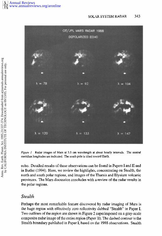
None of these limitations were operative when the first Mars VLA/Goldstoneradar experiments were performed in 1988; these yielded unambiguous maps ofthe entire observable hemispheres in two orthogonal modes of circular polariza-tion. This work was reported in Muhleman et al (1991), hereafter called Paper and in the thesis of Butler (1994), hereafter called Paper II (see also B utler et (1993)). The 27 antennas of the VLA operate N(N- 1) /2= 351(fN = 27) simultaneous interferometers, which discreetly sample the Fourierspatial components of the observed radio source. The antennas are in a "Y"configuration with a maximum separation of 36 km between the end membersof the Y for the experiments considered here. The 2-dimensional Fourier trans-form of the set of flux-density amplitudes and phases measured in each antennapair yields a 2-dimensional, unambiguous spatial map of the source convolvedwith the effective beam of the array. [See Thompson et al (1991) for a thoroughdiscussion ofinterferometric arrays.] As the source passes the observatory fromthe eastern to the western horizon, the projection of the individual antenna-pairbaselines rotate on the source and effectively fill the array aperture (depend-ing on source declination). However, because of the 24.62-h rotation of Mars,this rotational synthesis technique cannot be used in practice. Instead, Marswas observed in 12-15 minute snapshots, affording essentially zero baselinerotations. Because the exact positions of the antennas are known to a frac-tion of the 3.5-cm wavelength and the signal phases are accurately calibrated,the effective beam could be accurately deconvolved from the data, producingexcellent images as shown in Figure 1. The calibration of the data used thestandard technique of observing known point radio sources. Additional phaseself-calibration was achieved by using the specular spike in the polarized radar
Figure 1 meridian longitudes are indicated. The south pole is tilted toward Earth.
Radar images of Mars at 3.5 cm wavelength at about hourly intervals. The central
echo. Detailed results of these observations can be found in Papers I and I1 and in Butler (1994). Here, we review the highlights, concentrating on Stealth, the north and south polar regions, and images of the Tharsis and Elysium volcanic provinces. The Mars discussion concludes with a review of the radar results in the polar regions.
Stealth Perhaps the most remarkable feature discovered by radar imaging of Mars is the huge region with effectively zero reflectivity dubbed “Stealth” in Paper I. Two outlines of the region are shown in Figure 2 superimposed on a gray-scale composite radar image of the entire region (Paper 11). The dashed contour is the Stealth boundary published in Paper I, based on the 1988 observations. Stealth
was observed again in 1993 at near-normal incidence and the new contour based on all the data is indicated by the solid lines in Figure 2. It can be seen from the gray-scale image that very low reflectivity material continues westerly beyond the 170” meridian. The reflectivity limit for the 1988 data was 0.5% and that for the 1993 data was 0.25%. We define the “reflectivity” as the radar cross section per unit projected area. We computed it from the ratio of the reflected power in a given beam (in either polarization) to the total power that would be reflected from the unity reflector with the same cross-sectional area as the beam. Our reflectivities include both the electrical effects due to the surface material dielectric properties and the backscatter “gain” caused by surface roughness or multiple scattering effects. Stealth extends nearly 2500 km along the equator, with its east boundary at the base of the Tharsis volcanic ridge. Tentative explanations for this feature, which is unique among the terrestrial planets, are given in Papers I and 11, along with estimates of its composition and minimum depths of the underdense layer.
From a pure physics standpoint, Stealth is a region with a nearly perfect impedance match to free space. Of course, there is true reflection from it that is below the sensitivity of these short-wavelength experiments. JK Harmon (private communication, 1994) has obtained new observations at a wavelength of 13 cm that display the stealth effect but none of the details are published
Longitude
Figure 2 Radar image of the Stealth region on Mars shown in a cylindrical projection of the effective normal incidence S S reflectivity. The solid line shows the best estimate of Stealth from all 3.5-cm data; the dashed line is from Muhleman et a1 (1991). The Tharsis volcano calderea and shields are suggested by the while lines. (From Butler 1994.)
yet. RF Jurgens (private communication) has Goldstone observations of thestealth effect along the southern edge of the feature in 1992. It is clear thatStealth is made of material to some depth that both reflects very little centimeterwavelength energy and does not exhibit a significant reflection from its lowerboundary, which must be higher density material typical of the rest of theMartian surface. Furthermore, the medium is free of rocks and clumps ofcentimeter sizes and larger that would act as volume scatterers. The absenceof a sublayer reflection requires that the stealthy material has sufficient ohmicabsorption properties to suppress the reflection from the lower boundary, i.e.the layer possesses some opacity. If the mean depth of the layer is D and themean absorption coefficient per unit length is kv, the optical depth is
r = k~,D. (1)
Using the reasonable concept that the lower boundary is rough on the scaleof the wavelength, or equivalently, that the true depths vary significantly overan area on the scale of the pixels (or on the scale of the first Fresnel zone), theeffective reflectivity can be written
R! (1 - R0)2e-2rR = Ro + 1- RoRle-2r ’ (2)
where Ro is the power reflectivity of the surface layer material and R1 is theeffective reflectivity of the lower boundary interface. If the surface layer isinfinitely deep, the observed reflectivity is just R0, which must be less than0.0025 to match the upper limit from the observations. Since we have onlyobserved an absence of a radar reflector at this limit, the concept of a surfacegain has no meaning. Consequently, we tentatively interpret the limit of 0.0025as that of the electrical reflectivity for a smooth surface at normal incidence. Ifthe layer were perfectly transparent, i.e. ¯ = 0, Equation (2) yields
Rl(1 -- Ro)2R=Ro+ "" R~ + Ro,
(1 - RoRI)
where the approximation holds because R0 is very small in any case. If Stealthwere a homogeneous layer of infinite depth with a complex dielectric constantE = Er - i Ei, then the reflectivity as a function of the real part of the dielectricconstant would be that shown in Figure 3a. The three lines shown are for losstangents, tan(d) (Ei/Er) equal to0.005, 0.020, and0.045, and demonstratethat the reflectivity of a homogeneous half-space is practically independent ofthe absorption properties of the medium. The observed upper limit of the Stealthreflectivity of 0.0025 shows that such a half-space must have a real dielectricconstant less than about 1.25, i.e. it must be extremely underdense relativeto known surfaces on the terrestrial planets. The reflectivity computed fromEquation (2) with R0 ---- 0.0025 and R1 = 0.10 and 0.25 is shown in Figure 3b.
1.0 1.2 1.4 1.6 1.8 2.0Real Part of Dielectric Constant
(~)
2 4- 6 8 1 14
OPTICAL DEPTH OF LA¥£1~
Figure 3 Reflectivity model for Stealth. (a) The normal incidence reflectivity for an infinite half-space of a homogeneous dielectric medium with the real part of the dielectric constant. A rangeof imaginary parts is shown with the dashed line. (b) The normal incidence reflectivity of a layerover the averaged Mars surface as a function of the 3.5-cm optical depth of the layer. Dotted anddashed lines indicate a wide range of absorption coefficients.
It can be seen from the figure that for reasonable values of the Martian sublayerreflectivities of 10 and 25%, the 3.5-cm optical depth must be greater than5 or 6 to be consistent with the observations. Complimentary observationsfrom Arecibo at a longer wavelength (13 cm) should make it possible to betterestimate the minimum depths. A reasonable interpretation of this opacity hasyet to be offered.
It is well known that the electrical absorption coefficient for amorphous andcrystalline solids (nonmetals) is given
k~ -- ~x/~r tan(d), (3)
where ~. is the wavelength in the same units as D and tan(d) is the loss tangentof the material. Then from Equation (1) with > 5,theminimum depth Dcan be estimated for reasonable values of tan(d). Such values for estimates the complex dielectric constant of Martian soils are given in Paper I based onlaboratory measurements tabulated by Campbell & Ulrich (1969). For example,a soil made by grinding a "typical" Earth basaltic rock to a density of about1.0 gm cm-3 would have an E ’-, 2.0 - i0.016 (see also Muhleman & Berge1991 for further discussion). Such a soil packed with density of 0.4 gm cm-3
would possess E ~ 1.33 - i0.0043, a reasonable estimate of what is expectedfor Stealth. Using this value and Equations (1) and (3), we estimate a minimumdepth of D --~ 7.5 meters for the layer. This hypothetical basalt is actuallystrongly absorbing. Following Paper I, the value for a less mafic soil that iscertainly within the expected range for Mars is E -~ 1.33 - i0.00215, whichfor r = 5 gives D > 15 m. These calculation are highly idealized, and theuncertainties of the measurements suggest the minimum depth of the underdense layer could be as small as 2 or 3 m.
Our estimates of 7-15 m for the Stealth deposit (with density ,-~ 0.4 gm cm-3)
are nearly as remarkable as the lateral extent of the deposit. Nothing like thisexists on the Earth or is known to exist on the terrestrial planets or the Moon.The fact that the deposit lies to the west of the colossal Tharsis volcanic ridge inthe equatorial zone is very significant. Furthermore, the topography falls fromthe eastern boundary at about 8 km above the Mars reference datum to near 0km at the western boundary. Viking images of the ensemble of regions makingup Stealth have been studied by many investigators including Scott & Tanaka(1982), Cart (1984), and Schultz & Lutz (1988). The geological map of Scott Tanaka (1986) shows that much of the eastern and northern parts of Stealth liesin the upper and middle Medusae Fossae units. The east/west division in thefeature is related to the Mangala Valles region, which is a cratered area somewhatelevated relative to Medusae Fossae units. Most of the southern boundary ofStealth is labeled as "Highland-Lowland Boundary Scarp" in the geologicalmap. Scott & Tanaka have interpreted these units as ash-fall, ash-flow tuff,or thick eolian deposits. This interpretation was adopted by Muhleman et al
(1991), who suggested further that the ash flow may have originated fromthe Tharsis ridge volcanoes Arsea and Pavonis Montes. These volcanoes aresituated in the equatorial zone where the prevailing winds are thought to be fromeast to the west, similar to the tropical trade winds on Earth. This is consistentwith the general circulation calculations of Pollack and others. However, ifthe depths suggested here are correct, the materials must possess significantstrength against collapse. Roughly, a 7-m column of material at density 0.4gm cm-3 would have a base pressure of 280 gm cm-3 and cannot be "dust" andmay be in a welded form like pumice. Finally, it should be noted that the entireStealth region has been mapped as a region with very low thermal inertias; seeKieffer et al (1977) and Palluconi & Kieffer (1981).
Tharsis Volcanic Region
The Tharsis region includes the three shield volcanoes on the Tharsis Ridge:Arsia, Pavonis and Ascraeus Montes, and Olympus Mons--all structures oforder 25 km above the datum level of the planet. These, and a number ofother "old" volcanoes, surround the north and east boundaries of Stealth. Inaddition to the number of known remarkable characteristics of these structures,the VLA/Goldstone images reported in Papers I and II revealed important newfacts about the region. All four volcanoes have distinct radar features that arenearly the brightest on the planet, after that of the Residual South Polar Cap, soevident in Figure 1. Equally radar-bright are regions in the Elysium complexdiscussed below. Butler (1994) has developed a useful technique for combiningthe data from all of the snapshots in which a given feature is visible. A featurenear the equator is imaged over a wide range of look angles--angles of incidencecombined with the local azimuth angle toward the radar. He has assumed thatthe backscatter intensity for a given point on the surface can be represented bythe simple function
I (~, x, y) = A cosn ~b, (4)
where ~b is the incidence angle at time t, and x, y are the surface coordinates ofthe point. The reflectivity data for a given point were fit in a least-squares senseby adjusting A and n in Equation (4). A takes on the meaning of the reflec-tivity that would be observed at normal incidence at that point. The intensityI is effectively averaged over a pixel area in the final composite image of theresulting values of the parameter A, which are then normalized to reflectivityunits. One such composite map (for Stealth) is shown in Figure 2. Informa-tion is lost in this manner.because an average has been taken over a range ofazimuthal angles. A cylindrical projection of the SS data for the entire Tharsisand Elysium domains is shown in Figure 4. The shields and calderae of themajor volcanic structures from photographic images and geological maps areindicated by white lines in this figure. The reflectivities (which are really values
Figure 4 A cylindrical projection of the SS reflectivity of the entire Tharsis and Elysium regions. The contours are in 2.5% increments and the gray scale runs from -.4 to 24.6%. (From Butler 1994.)
of Ass, the reflection coefficient at normal incidence for SS polarization) are indicated both in gray scales and contour lines. A number of things are note- worthy in Figure 4. The low reflectivity region containing Stealth continues westward to south of the Elysium complex (roughly centered at 210"W, 20"N). All of the bright radar features are associated with the volcanoes, including the largest region in Daedalia Planum centered on 122"W, 21"s (called the "south Tharsis" in Paper I). Only the bright feature in Ascraeus Mons falls on the mapped position of the caldera, while the bright feature in Arsia Mons is on the edge of its caldera. These structures are more closely examined in the next paragraphs.
The details of Arsia Mons can be seen in the Ass map in Figure 5a. The dominant feature in this map is the huge anomaly directly south of the breach in the Arsia Mons caldera. The brightest pixels in this map have normal incidence reflectivities of Ass = 24.6% and Aos = 22.7% (at 122"W, 21"s) (Paper 11). These values should be compared to the the Martian mean values for the globe excluding the radar anomalies. When extrapolated to normal incidence these values become Ass = 1.5% and Aos = 4.0%, with a ratio of 0.37. The Viking images of this region (seep. 234 of Tyner & Carroll 1983) show that it is heavily grooved toward the southwest direction from the volcanic breach. It is tempting to interpret this grooved terrain as fresh lava flows because of its relationship to Arsia Mons, its extreme roughness, and its very high reflectivity. We know of no structure on the terrestrial planets or the Moon that approach these values except
for the ice on the Residual South Polar Ice Cap (RSPIC). Some ground truth does exist from Earth lava flows but these have considerably smaller numerical values (see Campbell et a1 1993 and the references therein). Of course, we cannot define the word “fresh,” but the results strongly suggest that the reflections are created by both maximum roughness, and possibly, by highly metallic lavas. The reflectivities near the caldera on Arsia Mons are also impressive with Ass = 15.8% and Aos = 13.0% at 120”W, 9”s (we doubt that the difference in these values is significant). Quite consistently, the polarization ratios in all the volcanic anomalies is near, or slightly greater, than unity. Although such values are possible for surface reflections from blocks whose random
Longitude
Figure 5 (n) Cylindrical projection of SS reflectivities for Arsia Mons. Contours and gray scales are the same as in Figure 4. (b) Same for Olympus Mons region, but the gray scales range from 2.25 to 17.4%. (From Butler 1994.)
orientations create good corner reflectors, they more likely result from multiplescattering of energy penetrating into the surface. The Viking images of ArsiaMons show nothing of obvious interest at this location (Tyner & Carroll 1983,pp. 238-39); however, the radar feature does lie on the back wall of the caldera.
The feature in Ascraeus Mons, which is even brighter, falls right in thecaldera (Ass = 34% and Aos = 22.7% at 104°W, ll°N). The Viking images,(Tyner & Carroll 1983, p. 128) suggest that the caldera is strongly broken is the superposition of a number of calderae. Again, the fundamental questionis: How recent was the last volcanic activity? The complexity of the reflectionphysics and the lack of ground-truth data make it very difficult to interpret theseresults. The radar anomalies on Olympus Mons (Ass "~ 17%) and on PavonisMons (Ass ~ 20%) are on the flanks of these volcanoes and are also strongscatterers. Apparently, these were created by more recent volcanic activity thanthat in the calderae, although the structure and texture of the lavas may havebeen different at the time of the flows. The Pavonis anomaly is on the edgeof the volcano’s shield, and its caldera is only moderately more reflective thanthe mean in Tharsis. The cylindrical projection of the Ass values for OlympusMons is shown in Figure 5b, where the photographed outline of the volcano isindicated by white lines. The two brightest features are essentially offthe shieldalthough the caldera is moderately bright. The feature centered on 117°W, 14°Nis actually on the west flank of the Tharsis ridge and may not be associated withOlympus Mons.
Elysium Complex
The Elysium complex was poorly viewed in the 1988 VLA/Goldstone exper-iments and was properly imaged in 1993. The 3.5-cm radar map appears inPaper II and is reproduced here in Figure 6. Again, the radar anomalous re-gions tend to be adjoining the principal volcanoes with a peak SS reflectivityof Ass = 20% (203°W, 20°N). The Elysium caldera is at 214°W, 25°N and,although there is no doubt that it is part of Elysium Mons, it may be incorrect toclosely associate the radar anomaly with this volcanic complex. The caldera ex-tends southeast from the volcano down the Elysium rise. Harmon et al (1992a)obtained images at Arecibo at 13 cm in 1990 and have published a single SSimage of the Elysium quadrant. They used the new long random code techniqueto image the surface without aliasing. The maps are in good agreement, and themajor differences may be due to the different way the data sets were projected.In particular, the Arecibo map suggests higher reflectivity than the VLA mapin the region called the Cerberus Formation by Plescia (1990). This structurecovers the region from the equator to about 10°N and is roughly bounded be-tween 180°W to 210°W. Harmon et al observed a bright, nearly linear featurein the northeast corner about 500 km long, which is prominent in Plescia’s mapbut not in the 3.5-cm data as projected in Figure 4.
Figure 6 A cylindrical projection of the SS reflectivities in the Elysium region. The contours are at 2.5% increments and the gray scale ranges from 1.5 to 20.3%. The white lines suggest the calderea flanks of Hecates Tholus to the north, Elysium Mons in the center, and Orcus Patera to the east. (From Butler 1994.)
The Arecibo group points out the close correspondence of their 13-cm map with the Cerberus Formation, which has been interpreted as a floodplain deposit; the more sinuous linear feature to the east is decribed as a “smooth-floored outflow channel” by Tanaka & Scott (1980) (see also Can & Clow 1981). Harmon et a1 (1992a) conclude that there is general agreement in the geological literature that the “Elysium Basin was the site of a paleolake and that the channel was an outlet for water flowing northeast into Amazonis.” However, this seems in clear conflict with the radar-brightness of the region at both 3.5- and 13-cm wavelength, which is very likely associated with lava flows and deposits. Plescia (1990) has interpreted this region, including the channel, as having been flooded by low-viscosity lava flows, postdating the fluvial episodes. This scenario is consistent with the radar data. The absence of clear evidence for the channel in Figure 4 at 3.5 cm is puzzling. While it may be a projection defect in the mapping, the possibility exists that other reflection mechanisms are operating if, indeed, the 13-cm reflections are significantly stronger. That could occur if the enhanced reflections were caused by volume scattering from buried rocks or lavas because the long wavelength energy could probe to 2-3 times the depth of the 3.5-cm signals in partially transparent materials such as very dry “sand.”
The first radar images of ice on Mars were made from the VLAJGoldstone 1988observations when the subradar point on Mars had a latitude of 24°S and theMartian longitude of the Sun was Ls = 295° (mid-southern summer). Six the 38 snapshot images are shown in Figure 1 where the prominence of the southpolar ice reflection is obvious. The SS reflectivity at the angle of incidence 66°
was reported to be essentially unity in Paper I and has been corrected to 85%in Paper II and in Butler et al (1993), hereafter called Paper III. The necessary
~ brings this value to 42%. The pixels with the very largecorrection factor of ireflectivities all lie on the RSPIC as seen in Viking and Mariner 9 photographs.This ice deposit behaves like a "white" screen, even at angles of incidencenear grazing. This requires the ice to be heterogeneous with cracks, voids,or condensations acting as scattering centers. The data were interpreted as thereflection from a multiply scattering medium, which is essentially conservativeat centimeter wavelengths, i.e. with a single scattering albedo essentially unity.The strong backscatter at grazing incidence angles was a surprise because it wasexpected that the ice (either water or carbon dioxide) would be homogeneous,either from annealing processes or ab initio as the ice was laid down in the formof frost. It was also shown in Paper I that the medium is essentially transparentand that scattering from rocks in the ice matrix could be ruled out, consistentwith conservative scattering.
The polar data were remapped by averaging the data from the snapshots,and the results for both the SS and OS data are shown as radar cross sectionsin Figure 7. The SS cross sections are nearly twice as high as the OS valuesfor the pixels on the RSPIC, which are marked with white lines. (SS valuesalso exceed the OS values in a kind of penumbra around the visible ice cap,caused by the projection technique.) The anomalous polarization ratios arealso found on the icy Jovian satellites as discussed earlier and appear to be aclear indicator of planetary ice, or at least, the presence of highly transparentmaterial at the relevant wavelength, such as very cold ice. Even the minimumthickness of the ice is nearly impossible to estimate with such meager data.The problem was modeled as a pile of spherical ice balls in Paper I, yielding aminimum thickness of about 1.6 m for ice spheres the size of the wavelengthpiled on top of each other. It was also modeled in Paper I as a suspension of suchscatterers in a transparent matrix, yielding about a 5-m thickness for separationsof about 25 cm between the scattering centers, an arbitrary value. The problemwas modeled somewhat more accurately in Paper III using a power-law sizedistribution in a similar Monte Carlo calculation. It was concluded that forthe epoch of observation the minimum thickness would have to be about 10 mif the Martian dust contamination of the ice was about 1%. The data andinterpretations clearly establish that the upper few meters of the ice sheet areremarkable clean and very heterogeneous, i.e. highly fractured or lumpy. It is
not at all clear why the ice on Mars is in this state, but annealing calculations reported in Paper I11 show that once the ice (assumed to be water) is in that state at the Martian poles, it will remain that way.
The north polar region has only been observed at the VLA and at a time when the grazing angle at the pole was just 9" to 6", dangerously low to observe the effects of the Residual North Polar Ice Cap (RNPIC), which is much more extensive than the RSPIC. The season was early spring with LS = 18.2" and 24.8", respectively-perhaps early for the sublimation of the seasonal COZ ice cap. The seasonal cap is estimated to be of order 1 m thick and should be essen- tially transparent to 3.5-cm energy even at an incidence angle of 81". However, the radar signature for ice was not seen! Cross-section images from Papers I1 and I11 are shown in Figure 8; the boundary of the RNPIC is indicated in white. Even though the RNPIC extends down to about the 80"N latitude circle where the grazing angle reaches about 18", no reflectivity enhancement due to ice is present. The putative ice deposits on Mercury were detected at a grazing angle of 13" as discussed below. Butler et a1 offer in Paper I11 several possible but un- convincing explanations for the newly found dichotomy between the two poles.
1. The grazing angles are too low for the RNPIC; the RSPIC was observed at 24".
2. The seasonal COz frost was still in place and tended to fill the voids, removing the heterogeneous dielectric structure.
ss os
Figure 7 Stereographic projection of the south polar SS (Iefi) and OS (right) cross sections. The contours are at reflectivities = 0.025, 0.05, 0. I , . . . , 0.4. The white lines represent the Residual South Polar Ice Cap. Ls - 295". (From Butler 1994.)
Figure 8 Stereographic projection of the north polar SS (lefr) and OS (right) cross sections. The contours are at reflectivities = 0.025 and 0.05. The white lines represent the Residual North Polar Ice Cap. Ls - 20". (From Butler 1994.)
3. The seasonal dust deposition in the north was sufficient to raise the absorp- tion properties of the matrix above a critical value to turn off the coherent backscatter effect.
4. The thermal environment at the north pole is sufficiently different from the south pole to allow much more efficient annealing of the ice fractures. For example, our knowledge of the topography at the poles is very poor but is likely to be relevant.
5 . The glacier-like ice flow is significantly different in the north than in the south. The ice could be more loaded with soil and rock debris, thereby creating more absorption.
This important problem remains unsolved and none of these mechanisms seems to be sufficiently robust to explain the striking observational dichotomy. Better measurements such as those promised from the ill-fated Mars Observer mission are required.
Radar astronomy of Mars has been a fountainhead for information about the planet and will continue to be important. Much higher resolution can be achieved on Mars with the VLNGoldstone radar. The observational technique using 12-15 minute snapshots was dictated by signallnoise considerations in the selection of the observing Doppler bandwidth. If a significant increase in transmitter power at Goldstone were achieved, narrower channels at the
VLA could be employed with increased east/west resolution, e.g. 2-5 minutesnapshots might be possible. The use of the long-code techniques at Arecibo(and with Goldstone in the monostatic mode) will yield more interesting Martianmaps, albeit, always plagued by the north/south ambiguity about the Dopplerequator. At the time of this writing, the transmitter power at Arecibo is beingsignificantly increased to 1 MW, and the surface will be considerably improved.The increase in the resolution of radar maps will be impressive. Finally, theradar globe of Mars is certainly different from the photographic globe because ofthe penetrating power of microwaves. It certainly can be argued that a Magellan-like mission to Mars would be very fruitful! Interestingly, we do not have aphotographic globe of Venus.
MERCURY
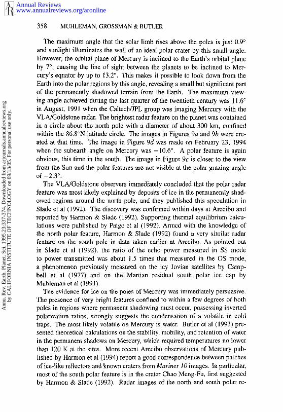
Mercury was first observed with the Goldstone radar by Carpenter & Goldstein(1963), observations both in the form of Doppler spectra and somewhat cruderange-gated spectra with range depths of 178 km. These observers misseddetecting the striking result that Mercury was not in synchronous rotation withits orbit about the Sun (87.97 day period) but was in a faster rotation with period of about 59 -t- 5 days, which was discovered at Arecibo by Pettengill(apparently first reported in Pettengill 1965). This result produced a flurry theoretical work by G Colombo, II Shapiro, P Goldreich, and S Peale, whichresulted in the realization that Mercury’s solid body rotation was locked in the~ spin resonance with its orbital motion and that the spin axis is very nearly2perpendicular to its orbital plane (see the review by Peale 1988). Unfortunately,the rotation period of 59 days means that Mercury spins too fast for range-gatedDoppler mapping to work well, and the planet remained essentially unmappeduntil the first VLA/Goldstone radar imaging experiment on August 8, 1991. Ofcourse, half of the surface of Mercury was photographed with resolution of afew kilometers from Mariner 10 in 1974 (see, in particular, Murray et al 1974).The Mariner results have been widely distributed in map and book forms suchas Davies et al (1978). The entire globe of the planet was imaged with theVLA/Goldstone radar at a wavelength of 3.5 cm. Four such images are shownin Figure 9. Figure 9a was the first image obtained (on August 8, 1991) whenthe north pole was tilted toward the Earth by 10.7°. At this angle the line ofsight was down into the north pole and the brightest echo from the planet wasaround this pole. The striking similarity between the images in Figures 9aand b (obtained 15 days later) with the images of Mars shown in Figure 1 wasimmediately suggestive of ice on the north pole of Mercury.
Mercury’s position as the innermost planet in the Solar System is sufficient tomake it unique since it presumably formed nearest the Sun. It has no satellite andhas evolved to a simple rotational state with its spin axis exactly perpendicularto its orbital plane to the accuracy of the measurements. If Mercury were a
smooth sphere, the Sun would never set on any point on the globe. A crescent Sun, modulated by the varying solar distance, would always be seen from the poles. However, the bottom of any crater exactly at the pole will be in perpetual shadow, warmed only by light scattered from the crater rim, heat conducted up from the planet’s interior, and cosmic “light.” Estimating just how cold these spots could be is very difficult and depends on the details of the crater, but temperatures as low as 30 K are possible. Temperatures on the Mercury nightside fall to about 90 K at the very surface. Craters known from Mariner 10 imaging of the then dayside of the planet would have permanently shadowed zones if they lie within about 5” of the pole and possibly even further. Cold traps for volatiles are also created on the poleward sides of ridges and certainly in cracks within about lo” from the poles.
Figure 9 Radar SS images of Mercury at four epochs: (a) April 8, 1991 with the north pole tilted toward the Earth, (b) April 23, 1991 with the north pole tilted toward the Earth, (c) November 23, 1992 with the subearth point nearly on Mercury’s equator (-2.3’). and (d) February 21, 1994 with the south pole tilted toward the Earth. (Copyright: BJ Butler, DO Muhleman, and MA Slade, 1994.)
The maximum angle that the solar limb rises above the poles is just 0.9°
and sunlight illuminates the wall of an ideal polar crater by this small angle.However, the orbital plane of Mercury is inclined to the Earth’s orbital planeby 7°, causing the line of sight between the planets to be inclined to Mer-cury’s equator by up to 13.2°. This makes it possible to look down from theEarth into the polar regions by this angle, revealing a small but significant partof the permanently shadowed terrain from the Earth. The maximum view-ing angle achieved during the last quarter of the twentieth century was 11.6°
in August, 1991 when the Caltech/JPL group was imaging Mercury with theVLAYGoldstone radar. The brightest radar feature on the planet was containedin a circle about the north pole with a diameter of about 300 km, confinedwithin the 86.8°N latitude circle. The images in Figures 9a and 9b were cre-ated at that time. The image in Figure 9d was made on February 23, 1994when the subearth angle on Mercury was -10.6°. A polar feature is againobvious, this time in the south. The image in Figure 9c is closer to the viewfrom the Sun and the polar features are not visible at the polar grazing angleof -2.3°.
The VLA/Goldstone observers immediately concluded that the polar radarfeature was most likely explained by deposits of ice in the permanently shad-owed regions around the north pole, and they published this speculation inSlade et al (1992). The discovery was confirmed within days at Arecibo andreported by Harmon & Slade (1992). Supporting thermal equilibrium calcu-lations were published by Paige et al (1992). Armed with the knowledge the north polar feature, Harmon & Slade (1992) found a very similar radarfeature on the south pole in data taken earlier at Arecibo. As pointed outin Slade et al (1992), the ratio of the echo power measured in SS modeto power transmitted was about 1.5 times that measured in the OS mode,a phenomenon previously measured on the icy Jovian satellites by Camp-bell et al (1977) and on the Martian residual south polar ice cap Muhleman et al (1991).
The evidence for ice on the poles of Mercury was immediately persuasive.The presence of very bright features confined to within a few degrees of bothpoles in regions where permanent shadowing must occur, possessing invertedpolarization ratios, strongly suggests the condensation of a volatile in coldtraps. The most likely volatile on Mercury is water. Butler et al (1993) pre-sented theoretical calculations on the stability, mobility, and retention of waterin the permanent shadows on Mercury, which required temperatures no lowerthan 120 K at the sites. More recent Arecibo observations of Mercury pub-lished by Harmon et al (1994) report a good correspondence between patchesof ice-like reflectors and known craters from Mariner 10 images. In particular,most of the south polar feature is in the crater Chao Meng-Fu, first suggestedby Harmon & Slade (1992). Radar images of the north and south polar re-
www.annualreviews.org/aronlineAnnual Reviews
Ann
u. R
ev. E
arth
. Pla
net.
Sci.
1995
.23:
337-
374.
Dow
nloa
ded
from
arj
ourn
als.
annu
alre
view
s.or
gby
CA
LIF
OR
NIA
IN
STIT
UT
E O
F T
EC
HN
OL
OG
Y o
n 09
/13/
05. F
or p
erso
nal u
se o
nly.
SOLAR SYSTEM RADAR 359
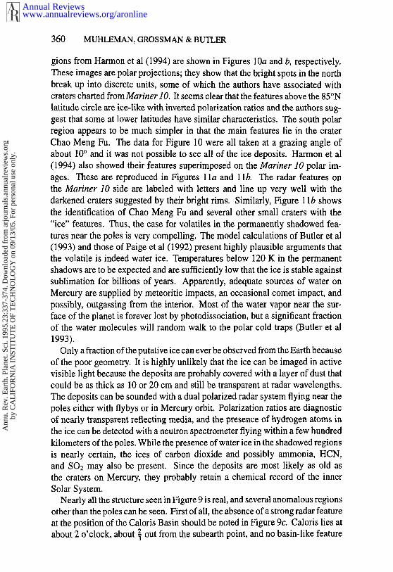
Figure 10 a wavelength of 12.6 crn from Harmon et a1 (1994). Latitude circles of 80' and 85' are shown.
Radar delay-Doppler radar images of the (u) north and (b) south poles of Mercury at
gions from Harmon et al (1994) are shown in Figures 10a and b, respectively.These images are polar projections; they show that the bright spots in the northbreak up into discrete units, some of which the authors have associated withcraters charted from Mariner 10. It seems clear that the features above the 85°Nlatitude circle are ice-like with inverted polarization ratios and the authors sug-gest that some at lower latitudes have similar characteristics. The south polarregion appears to be much simpler in that the main features lie in the craterChao Meng Fu. The data for Figure 10 were all taken at a grazing angle ofabout 10° and it was not possible to see all of the ice deposits. Harmon et al(1994) also showed their features superimposed on the Mariner 10 polar im-ages. These are reproduced in Figures 1 la and 1 lb. The radar features onthe Mariner 10 side are labeled with letters and line up very well with thedarkened craters suggested by their bright rims. Similarly, Figure 1 Ib showsthe identification of Chao Meng Fu and several other small craters with the"ice" features. Thus, the case for volatiles in the permanently shadowed fea-tures near the poles is very compelling. The model calculations of Butler et al(1993) and those of Paige et al (1992) present highly plausible arguments the volatile is indeed water ice. Temperatures below 120 K in the permanentshadows are to be expected and are sufficiently low that the ice is stable againstsublimation for billions of years. Apparently, adequate sources of water onMercury are supplied by meteoritic impacts, an occasional comet impact, andpossibly, outgassing from the interior. Most of the water vapor near the sur-face of the planet is forever lost by photodissociation, but a significant fractionof the water molecules will random walk to the polar cold traps (Butler et al1993).
Only a fraction of the putative ice can ever be observed from the Earth becauseof the poor geometry. It is highly unlikely that the ice can be imaged in activevisible light because the deposits are probably covered with a layer of dust thatcould be as thick as 10 or 20 cm and still be transparent at radar wavelengths.The deposits can be sounded with a dual polarized radar system flying near thepoles either with flybys or in Mercury orbit. Polarization ratios are diagnosticof nearly transparent reflecting media, and the presence of hydrogen atoms inthe ice can be detected with a neutron spectrometer flying within a few hundredkilometers of the poles. While the presence of water ice in the shadowed regionsis nearly certain, the ices of carbon dioxide and possibly ammonia, HCN,and SO2 may also be present. Since the deposits are most likely as old asthe craters on Mercury, they probably retain a chemical record of the innerSolar System.
Nearly all the structure seen in Figure 9 is real, and several anomalous regionsother than the poles can be seen. First of all, the absence of a strong radar featureat the position of the Caloris Basin should be noted in Figure 9c. Caloris lies at
2about 2 o’clock, about .~ out from the subearth point, and no basin-like feature
Figure I I Superposition of 12.6-cm Mercury polar features over Mariner 10 photographic images, limited to the hemisphere of Mercury imaged: ( a ) north pole, (b) south pole. The Mariner images have been slightly translated. (From Harmon et al 1994.)
can be seen although there is apparently a slight enhancement in the region. Twolarge anomalies are obvious in Figure 9b, just to the astronomical west (right)of the central meridian. The southern feature is better seen in Figure 9d whereit is rotated to lower incidence angles. The next brightest anomaly is in theregion containing the bright rayed crater Kuiper, well imaged by Mariner 10.The radar anomaly is best seen in Figure 9d, just east of the subearth point.We limit our discussion to just these three features: the Kuiper region and theNorth and South Radar Basins.
Radar SS cross sections of the Kuiper region and a Mariner 10 image tothe same scale are shown in Figure 12. A circle representing Kuiper itselfis indicated in Figure 12~ along with the very bright contours relative to thesurrounding terrain with about 1.5% cross section at the angle of incidence
Longi~.ude (deg)40 35 30 25 20
0 I I I
-5
-10
-15
~ ~2.2%
Background -1.5 + .25%
Otne " 16~6
I I I
Figure 12 The Kuiper region on Mercury. (a) Contour lines of the SS reflectivity in a cylindricalprojection. The surrounding region has an average SS reflectivity of ~1.5%. The Kuiper crater isindicated by the dashed circle. (b) A Mariner 10 image of the Kuiper region to the same scale asthat in (a).
at Kuiper of 15.6" (the data have not been corrected for a scattering law). The brightest feature is not on the crater but lies about 160 km to the east in what looks like rough terrain in Figure 12b. Like Caloris, the bright Kuiper crater is not a strong backscatterer and may have a smooth floor and walls on the scale of the wavelength. The image resolution is about the size of the 3% contour in Figure 12a and we cannot expect to resolve an echo en- hancement from the far (east) wall of Kuiper although the small 2.5% contour may be related to that phenomenon. Higher resolution radar imaging of the region is required to better understand the relationship between the visually bright impact crater and the radar anomaly. Kuiper is similar to Tyhco on the Moon but the radar anomaly associated with Tycho is much smaller than that .of Kuiper.
Much larger still are the North and South Radar Basins. The North Basin SS contours are shown in Figure 13, taken from the August 23, 1991 image of Figure 9b. The image is a cylindrical projection and the angle of incidence from the subearth point to the brightest point in the feature is 44". If the 2.5% contour is corrected with a cosine scattering law, it becomes 3.5% and
is both brighter and much larger than the Kuiper basin. The North Basin waswell imaged in OS polarization. It looks very similar to the SS image with apolarization ratio of about 0.5 (Butler 1994), which strongly suggests that thebasin is either extremely rough (blocky) or is a medium that exhibits nearlyisotropic radar scattering [see Tryka & Muhleman (1992) for a discussion such structures]. Unfortunately, there is no ground truth for this side of Mercury.The South Radar Basin is even larger, as shown in Figure 14, but has similarradar cross sections and polarization ratios. The feature is about the same sizeas the Caloris Basin but is extremely radar rough. Again, this may be causedby blockiness on the scale of the wavelength or may be a texture quality of thescattering medium. The centroid of the South Basin is located at about -29°
south and about 349°W longitude, placing it near the antipodal point of theCaloris impact basin, which is roughly centered on 30°S and 15°W, as pointedout by Butler et al (1993). Hughes et al (1977) has suggested that seismicfocusing of the Caloris event could have highly fractured the surface at theantipode. Such events could have conceivably created the scattering mediumresponsible for the radar basins.
r,ongit.ude (deg)
360 350 340 330 32065 ’ , ,
55
45
35
North BasinPeak: 55°N, 348WBackground -1 ±.25%
0in c = 44~2
Figure 13 The North Basin radar feature. Contour lines of the SS refleetivity are shown in acylindrical projection. The surrounding region has SS reflectivity ~1.5%. No Mariner 10 imagesexist for this hemisphere.
Figure 14 The South Basin radar feature. Contour lines of the SS reflectivity are shown in acylindrical projection. The surrounding region has SS reflectivity ~1.5%. No Mariner 10 imagesexist for this hemisphere.
TITAN
Titan, the largest satellite of Saturn, has taken on a central role in planetaryscience because it presents as many enigmas as any planet in the Solar System.Our current knowledge of the satellite is reviewed in Hunten et al (1984), andLunine (1994) has written a recent review on the Titan atmosphere, focusingon central unanswered questions. Little is known about the surface of Titanbecause optically thick clouds and hydrocarbon aerosols completely obscure thesurface from view at visual wavelengths. The atmosphere becomes transparent(opacity less than unity) at wavelengths longward of about 1 cm, although recentevidence suggests that there may be a partially transparent window near 1/zm,which allows some surface emission to be observed (see Griffith et al 1991and Griffith 1993). Thus, the surface can only be imaged remotely with radar,although surface microwave emission averaged over the mean disk has beenstudied by Grossman & Muhleman (1995). Convincing theoretical argumentssuggest that Titan’s rotation is synchronous with its orbital period about Saturn
of 15.94542 days. However, both the period and the orientation of the spinaxis remain unconfirmed by direct measurements. In principle, these quantitiescan be measured with radar techniques, given sufficient signal. Hubbard et al(1993), in the analysis of the massive data set from the occultation of 28 Sgr Titan, reported that the upper atmosphere, though distorted by zonal winds oforder 100 m sec-~, "shows substantial axial symmetry" with a position angleof the axis within -’q° of Saturn’s. i.e. perpendicular to Titan’s orbital plane.Such winds are super-rotational if the rotation period is 16 days.
Titan offers an extremely difficult radar target. In addition to being the mostdistant object detected by radar, during the past two decades the Saturn systemhas been deep in the southern sky at low declinations. It will not reach northerndeclinations near closest approach to the Earth until October, 1997. Thus, thesource has been invisible to Arecibo and has had short transits over Goldstoneand the VLA, amounting to a little more than twice the radar round-trip light-time of 2.5 h. At best, the full disk echo signal from Titan is 4.5 orders ofmagnitude weaker then Mercury’s disk, not allowing for the much shorterintegration times available for signal detection. The surface is expected to becomposed of ices contaminated by solid and liquid hydrocarbons but essentiallynothing is known about differentiation of heavier materials such as silicates andother meteoric material. The bulk density is 1.881 gm cm3, similar to that ofGanymede and Callisto.
Echoes from Titan were first obtained in June, 1989 by Muhleman et al(1990) using the VLA/Goldstone radar configuration. The diameter of Titan(5150 Km) subtends an angle of just 0.89 arc see at 8 AU, which can barelybe resolved with the VLA in its largest configuration at a wavelength of 3.5cm. Since only the 351 antenna-pair cross products are measured and not thetotal echo power in each of the 27 antennas, there is a serious loss in sensitivityand resolved measurements have not yet been made. If the rotational period isnear 16 days, then the maximum Doppler spreading of the echo is about 1300Hz. Additionally, if the surface is as radar rough as the icy Jovian satellites, theecho energy is expected to be broadly spread to the full Doppler width. Theinitial experiments determined that, indeed, the echo was broad and thus thatthe surface is radar rough (Muhleman et al (1990). Several attempts weremade to detect the echo from Titan using the Goldstone monostatic radar,and a reasonable Doppler spectrum was obtained after averaging over severaldays, verifying the broad limb-to-limb spreading of the echo (RM Goldstein RF Jurgens, private communication, 1992).
A major motivation for the Titan radar experiments was the putative globalocean of liquid hydrocarbons (ethane/methane) put forward by Lunine et (1983). They postulated that a surface reservoir up to several kilometers deepwas required to resupply the methane currently in the atmosphere, which isirretrievably destroyed by photodissociation. Furthermore, hydrocarbons such
as ethane, acetylene, and methane must condense out of the atmosphere belowthe cold trap at the tropopause and "rain" down on the surface. Such a globalocean was ruled out in the initial experiment because the strong echo detectionswere about an order of magnitude greater than what would be obtained from asurface of nonpolar hydrocarbons. Additionally, the nearly Lambertian radarscattering from the surface is strongly inconsistent with a smooth, liquid surface.Essentially nothing is known about Titan’s topography except that the cutoffradius of two radio occultation chords on opposite sides of the satellite wereidentical to within 500 m (Lindal et al 1983).
The authors of this review have carried out VLA/Goldstone radar experimentsnear the time of each closest approach of the Saturn system since 1989, obtaininga number of clear results and some puzzling ones. Much of this work waspresented in Muhleman et al (1993). Titan observations were made by operatingthe transmitter from the time of Titan rise at Goldstone to 2.5 h before itssetting at the VLA, yielding about 5 h total observing time on Titan, exceptfor about 10% overhead used to observe calibrator sources. Under the bestconditions, when the transmitter was operating at a maximum of 450,000 Wand the weather was dry at the VLA, the Titan radar spectrum was measuredin 381-Hz channels with a signal-to-noise ratio of 3-5 in a 5-hour track, i.e.solid detections could be made but with only marginal measurements of surfaceproperties. Furthermore, observations during 1989-1992 were complicated bywhat we now believe were occasional pointing errors as large as the half-power beamwidth of the 70-m antenna, which resulted in a decrease in themeasured reflectivities. For example, a 30 arc sec pointing error would causethe measured radar cross section to be depressed to 0.8 of the correct value.There is no method to check the pointing while the antenna is transmitting anderrors of this size and larger may have occurred during Titan experiments. Aswe show below, new antenna pointing curves for Goldstone were available forthe 1993 measurements, and indeed, the result are more consistent from day today. Nevertheless, we cannot rule out the possibility that the fluctuations in theearly data are real and possibly caused by large "lakes" of liquid hydrocarbons orother inhomogeneities on the surface. Certainly, the largest of the fluctuationsin the measured cross sections can not be caused by pointing errors and areprobably real effects associated with regions of increased roughness or cleanersurface ice, possibly ice mountains.
Radar cross-section values have been computed by estimating the total powerin the Doppler spectra divided by the power that would be received from asmooth, conducting sphere at the same distance and size of Titan. Thus, thecross sections are normalized by the cross-sectional area of Titan. At varioustimes, Titan was observed with either 381-Hz channels or 762-Hz channels,the latter to measure both circular polarizations. A cosn power law was fit tothe narrow channel data to integrate the total power for these experiments. The
cross-section results for all of the measurements are shown in Table 1. Trans-mitter logs always indicate that the transmitter was in the RCP mode. The VLAarray configuration is indicated as B, C, or D. The A array, being the largest,over-resolves Titan. The B array resolved it down to .85% and the D array wasso small that antenna shadowing occurred, requiring extensive data editing.Additionally, in the D array, confusing flux from Saturn affected the data dueto the large synthesized beam (7.2 arc sec). The optimum array configurationfor Titan is C, which does not resolve the satellite and suffers no antenna shad-owing. The tabulated longitudes assume that Titan is in synchronous rotation.The tabulated errors are those in estimating the cross sections and must not be
confused with the detection uncertainties, which are much smaller and involveboth the visibility amplitudes and phases.
Large variations can be seen in the early experiments, particularly in theD-array data, in part caused by confusion with Saturn’s thermal emission. TheSS polarization measurements are completely mysterious. Often no signalwas detected in RCP, except on 23 July, 1990 and August 11, 1992 when theSS cross sections were larger than the OS cross sections. We believe thatthe measurements are real and not the result of instrumental errors becausethere have been no false polarization measurements in our experiences withMercury, Mars, or Venus, which are essentially identical experiments exceptfor the signal-to-noise ratio. Because the 1993 observations are so extensiveand, apparently, the pointing of the transmitter was improved, we concentratethe remaining discussion on these data. The average spectrum for that year(excluding the 3 rainy days at the VLA) is shown in Figure 15. Our best estimateof the mean Titan radar cross section is 0.125 q- 0.02. The Doppler spectralshape is well represented by a cos1"4 ~b, where ~b is the angle of incidence. As
proof that these experiments are never perfect, it was necessary to remove afrequency offset from the data, apparently caused by a synthesizer setting error.Titan backscattering is even flatter than a Lambertian surface (n = 2), whichmakes it difficult to understand the daily cross-section variations if the rotationis as slow as the 16 day synchronbus period. Furthermore, such flat surfaces(seen on the icy Galilean satellites) suggest either high surface roughness nearly isotropic scattering from partially transparent media, and they shouldexhibit nearly random polarization. This was observed on only 2 of 8 days inwhich polarization measurements were made.
Cross sections plotted as a function of longitudes for synchronous rotationare shown in Figure 16 from all the experiments. The 1993 results are shownas filled points. Except for the 3 days when it rained at the VLA, the resultsare rather constant with a suggestion of higher reflectivity at the eastern, orapproaching elongation (0.15 -I- 0.05) than at the western elongation (0.10 q-0.04). The mean value of the cross section is then 0.125 4-0.02. Muhleman et al(1992) have speculated that the rotational rate of Titan may be slightly faster
TITAN RADAR SPECTRUMAvg. of Aug. 4,5,6,7,8 and 12,13, 1993
’’~’1 .... / .... I .... I .... I .... I
20
10
-, -3 -2 -1 0 1 2 3Channel Number
Figure 15 Radar spectrum of Titan at a wavelength of 3.5 cm, averaged over 7 days. The dashedline shows a cosl’4 ~b fit, where ~b is the angle of incidence. An adjustment was also made for asynthesizer offset of 88 Hz. The data show that the Titan surface scatters the radar signal similarlyto that from a Lambert sphere. (From Muhleman et al 1993.)
Z
OS POLARIZATION
50 100 150 200 250 3OO 350
TITAN LONGITUDE (DEC)
Figure 16 Measured OS radar cross sections of Titan at 3.5-cm wavelength, plotted as a functionof the Titan longitudes assuming Titan to be in synchronous rotation. The filled points are from1993. The mean of these data is 0.125 (0.010). (From Muhleman et al 1993.)
than synchronous, partly because of the rather large orbital eccentricity of 0.029.A period of 15.911 days, compared with a synchronous period of 15.9454 days,would change the longitude system to force the regions of observed high radarcross sections to be aligned. This new system puts the bright region at alongitude that was unobservable in the 1993 experiment! Thus, nothing newwas learned about the existence of this bright longitude or the rotation periodin the most recent experiment. However, we believe that our measurementsprovide a weak argument (at best) for other than synchronous rotation.
The measured mean refleetivity of Titan is similar to that of Callisto, ex-cept for the ambiguous polarization observations. The 3.5-cm cross section of0.30 4- .02 from Ostro et al (1992) is thought to be consistent with the dirtyice on Callisto’s near surface, which depresses its geometrical visual albedoto about 0.22 compared to those of Europa and Ganymede, which are about0.8 and 0.5, respectively (Johnson & Pilcher 1977). Thus, the collection Titan radar data to date suggests that the surface of Titan is most like that ofCallisto. This correspondence is well illustrated by a figure from Grossman &Muhleman (1995) reproduced here in Figure 17. Measurements for Solar Sys-tem bodies of radar cross sections are plotted against the microwave emissivityas determined by brightness temperature measurements. The mean value fromthe 1993 data was used for the cross section of Titan. The solid line indicates
~..EUROPA
GANYMEDESATURN’S RINCS ~. I
~. _CALLISTO
~ ITAN
MOON-~,.
EMISSI~TY
Figure 17 A rough plot of the centimeter wavelength radar cross sections of icy bodies (plusthe Moon) against the centimeter emissivity of the objects. The solid line at 45° shows thecomplimentary relationship between the two variables near which the data should full. (FromGrossman & Muhleman 1995.)
the complementary nature of the two measurements, i.e. that the emissivityand reflectivity should nearly add to unity. This relationship is not expected tostrictly hold for our observations because although emissivity is an integratedquantity, measured over all angles, the radar reflectivity is measured just in thebackscatter direction. The albedo and radar darkening on Callisto are not un-derstood but may be caused by silicates. A similar effect may exist on Titan butit is reasonable to expect that its surface is partially covered by low reflectivityhydrocarbon solids and liquids in the form of "lakes."
The Titan rotational direction and spin axis orientation will be determinedfrom future VLA radar measurements. Pinning down the exact rotational rateis much more difficult for it requires observing Titan continuously over severalorbits and correlating radar features, This may be possible with the upgradedAercibo radar. Furthermore, the atmospheric window at wavelengths near 1micron may provide data that will resolve this question in the next few years.
SUMMARY
Radar astronomy techniques continue to improve, making new and more uniqueexperiments possible. The radar facilities at Goldstone can be greatly improvedby feasible but expensive increases in transmitter power. That would make theVLA radar configuration far more valuable, allowing snapshots of Mars in acouple of minutes and making use of the highest resolution in the A arraypractical for Titan and the Galilean satellites. Since the Goldstone radar canscan the entire sky, it is the primary instrument for observing sources such asasteroids and comets in the southern sky or out of the ecliptic. The Areciboradar is being rebuilt as we write. It will bring radar astronomy into a new era.
Any Annual Review chapter, as well as any article cited in an Annual Review chapter,may be purchased from the Annual Reviews Preprints and Reprints service.
Butler BJ. 1994. 3.5-cm Radar investigationof Mars and Mercury: planetological im-plications. PhD thesis. Calif. Inst. Technol.,Pasadena (Paper II)
Butler B J, Muhleman DO, Slade MA. 1993.Mercury: full disk radar images and the de-tection and stability of ice at the North Pole.J. Geophys. Res. 98:15,003-23 (Paper III)
Campbell DB, Arvidson RE, Shepard MK.1993. Radar polarization properties of vol-canic and playa surfaces: applications to ter-restrial remote sensing and Venus data inter-pretation. J. Geophys. Res. 98:17,099-113
Campbell DB, Chandler JF, Ostro S J, PettengillGH, Shapiro II. 1977. Galilean satellites:1976 results. Icarus 34:254-67
Campbell MJ, Ulrichs RM. 1969. Electricalproperties of rocks and their significance forlunar radar observations. J. Geophys. Res.74:5867-81
Harmon JK, Slade MA, Hudson RS. 1992b.Mars radar scattering: Arecibo/Goldstone re-suits at 12.6-cm and 3.5-cm wavelengths.Icarus 98:240-53
HarmonJK, Slade MA, Velez RA, Crespo A,Dryer MJ, Johnson JM. 1994. Radar map-ping of Mercury’s anomalies. Nature 369:213-15
Harmon JK, Sulzer MP, Perillat P J, Chandler JE1992a. Mars radar mapping: strong backscat-ter from the Elysium basin and outflow chan-nel. Icarus 95:153-56
Hubbard WB. et al. 1993. The occulatation of 28Sgr by Titan. Astron. Astrophys. 269:542-63
Hughes HG, App FM, McGetchen T. 1977.Global seismic effects at basin-forming form-ing impacts. Phys. Earth Planet. Inter.15:251--63
Hunten DM, Tomasko MG, Flaser FM, Samuel-son RE, Strobel DE, Stevenson DJ. 1984. InSaturn, ed. T. Gehrels, MS Matthews, pp.671-759. Tucson: Univ. Ariz. Press
Johnson JV, Pilcher CB. 1977. Satellite spec-trophotometry and surface compositions. InPlanetary Satellites, ed. J Bums, pp. 232-68.Tucson: Univ. Ariz. Press
Thermal and albedo mapping of Mars duringthe Viking primary mission. J. Geophys. Res.82:4249
Lemmon MT, Karkoschka E, Tomoasko M.1993, Titan’s rotation: surface features ob-served. Icarus 103:329-32
Lindal GF, Wood GE, Hotz HB, Sweemam DN,Eshleman VR, Tyler GL. 1983. The atmo-sphere of Titan: an analysis of the Voyager1 radio occultation measurements. Icarus53:348-63
Lunine JI. 1994. Does Titan have oceans? Am.Sci. 82:134-43
Lunine JI, Stevenson DJ, Yung YL. 1983.Ethane ocean on Titan, Science 222:1229-30
Muhleman DO, Berge GL. 1991. Observa-tions of Mars, Uranus, Neptune, Io, Europa,Ganymede, and Callisto at a wavelength of2.66 mm. Icarus 92:263-71
Muhleman DO, Butler B J, Grossman AW, SladeMA. 1991. Radar images of Mars. Science253:1508-13 (Paper I)
Muhleman DO, Goldstein RM, Carpenter R.1965. A review of radar astronomy. Part 1.IEEE Spectrum 2:44-55; Part 2.2:78-89
MurrayBM, Belton MJS, Danielson GE, DaviesME, Gault DE, et el. 1974. Mercury’s sur-face: preliminary description and interpre-tation from Mariner 10 pictures. Science185:169-79
Ostro SJ. 1982. Radar properties of Europa,Ganymede and Callisto. In Satellites ofJupiter, ed. D. Morrison, pp. 213-36. Tucson:Univ. Ariz. Press
Ostro S J, Campbell DB, Simpson RA, Hud-son RS, Chandler .IF, et el. 1992. Eoropa,Ganymede, and Callisto: new results fromArecibo and Goldstone. J. Geophys. Res.97:18,227--44
OwenTC, Roush TL, Cruikshank DP, ElliotJL, Young LA. 1993. Surface ices and theatmospheric composition of Pluto. Science261:745
Paige DA, Wood SE, Vasavada AR. 1992. Thethermal stability of water ice at the poles ofMercury. Science 258:643-46
Pallueoni FD, Kieffer HH. 1981. Thermal inertiamapping of Mars from 60°S to 60 °N Icarus45:415-26
Peale SJ. 1988. The rotational dynamics of Mer-cury and the state of its core. In Mercury, ed.