Page 1
rILL WeAY
RADC-TR-87-44 IFinal Technical Report
(%jMay 198700
'mmv
cCOMPUTER ANAL YSIS OF ARBITRARIL YTAPERED RECTANGULAR ANDDOUBLE-RIDGED WA VEGUIDES
University of Utahp
Brett G. Braatz P
APPROVED FOR PUBLIC RELEASE, DISTRIBUTION UNLIMITED
ROME AIR DEVELOPMENT CENTERAir Force Systems Command
Griffiss Air Force Base, NY 13441-5700
Page 2
,. . . .•
report has been reviewed by the RADC Public Affairs Office (PA) and-'r-'.is releasable to the National Technical Information Service (NTIS). At NTIS
-"will be releasable to the general public, including foreign nations.
RADC-TR-87-44 has been reviewed and is approved for publication.
APPROVED: -
ANDREW E. CHROSTOWSKI, Capt, USAFProject Engineer
0. APPROVED: .4 -A-'
FRANK J. REHMTechnical DirectorDirectorate of Surveillance
FOR THE COMMANDER:
JOHN A. RITZ
Directorate of Plans & Programs
:!i
If your address has changed or if you wish to be removed from the RADC mailinglist, or if the addressee is no longer employed by your organization, please
notify RADC (OCTP) Griffiss AFB NY 13441-5700. This will assist us in
maintaining a current mailing list.
Do not return copies of this report unless contractual obligations or notice
on a specific document requires that it be returned.
II , '---------------- --i,-%, ---""':-L-'.'"... '".. -. ".."""-" " ] ,"""-",,..,".-'"-
! ~~~.. .-----.-.-. ,...- ".. -. _' ,. _ .... .... s, ,lf4,~' ' -' ' ', l Uw ml l
Page 3
UNCLASSIFIEDSECURITY CLASSIFICATION OF THIS PAGE
Form Approved
REPORT DOCUMENTATION PAGE oMSNo. 0704-0o 8
Ia. REPORT SECURITY CLASSIFICATION lb. RESTRICTIVE MARKINGS
UNCLASSIFIED N/A2a. SECURITY CLASSIFICATION AUTHORITY 3. DISTRIBUTION /AVAILABILITY OF REPORTN/A Approved for public release; distribution2b. DECLASSIFICATION / DOWNGRADING SCHEDULE unlimited.
4. PERFORMING ORGANIZATION REPORT NUMBER(S) S. MONITORING ORGANIZATION REPORT NUMBER(S)
UTEC MD-86-108 RADC-TR-87-44
68. NAME OF PERFORMING ORGANIZATION 6b. OFFICE SYMBOL 7a. NAME OF MONITORING ORGANIZATION(if applicable)Universfty of Utah Rome Air Development Center (OCTP)
6c. ADDRESS (City, State, and ZIPCode) 7b. ADDRESS (City, State, and ZIP Code)Department of Electrical EngineeringSalt Lake City UT 84112 Griffiss AFB NY 13441-5700
,a. NAME OF FUNDING/SPONSORING 8b. OFFICE SYMBOL 9. PROCUREMENT INSTRUMENT IDENTIFICATION NUMBERORGANIZATION (If applicable)
AFOSR NE F30602-82-C-0161
B.. ADDRESS (City, State, and ZIP Code) 10. SOURCE OF FUNDING NUMBERSPROGRAM PROJECT TASK WORK UNIT
Bolling AFB ELEMENT NO. NO. NO ACCESSION NO.Wash DC 20332 61102F 2305 J9 16
11. TITLE (Include Security Classification)
COMPUTER ANALYSIS OF ARBITRARILY TAPERED RECTANGULAR AND DOUBLE-RIDGED WAVEGUIDES
12. PERSONAL AUTHOR(S)
Brett G. Braatz13a. TYPE OF REPORT 13b. TIME COVERED 14. DATE OF REPORT (Year, Month, Day) 15. PAGE COUNT
Final * FROM R R TOP 2T May 1987 14016. SUPPLEMENTARY NOTATION Research was accomplished in conjunction with Air Force ThermionicsEngineering Research Program (AFTER) AFTER-21. Brett G. Braatz was an AFTER student fromTeledyne Microwave Electronics. This report was submit-pd_4n nnrtll (See Reverse)17. COSATI CODES 18. SUBJECT TERMS (Continue on revete if necessary and identify by block number)
FIELD GROUP SUB-GROUP Microwave Tubes Ridged Waveguide09 03 1Output Couplers Computer Analysis
I Tanered Havu der19. ABSTRACT (Continue on reverse if necessary and identify by block number)
The presented work was motivated by a need for high-power, wideband waveguide transitionswith low VSWR to be used as output couplers of microwave tubes. The work consists of acomputer analysis of arbitrarily tapered waveguides with ridged and unridged cross sections.The analysis combines coupled mode theory with numerical methods to solve nonuniform wave-guide problems. The coupling coefficients in Solymar's form of the generalized telegraphist'sequations are computed from numerically obtained eigenvalues and eigenfunctions. Thescattering matrix for a section of tapered waveguide is obtained by solving the coupleddifferential equations once for each initial mode amplitude in a complete orthogonal set.
.SNI The method can be applied to multimode problems with arbitrary cross sections and taperedshapes. The technique's usefulness is demonstrated for dominant mode rectangular and ridgedwaveguides having linear and cosine tapers. It is shown that the theoretical prediction ofVSWR agrees well with experimentally obtained results. .,-
20. DISTRIBUTION/AVAILABILITY OF ABSTRACT 21. ABSTRACT SECURITY CLASSIFICATION
"UNCLASSIFIED/UNLIMITED C3 SAME AS RPT. DTIC USERS UNCLASSIFIED22s. NAME OF RESPONSIBLE INDIVIDUAL 22b. TELEPHONE (Include Area Code) 22c. OFFICE SYMBOL
Andrew E. Chrostowski. Cant. USAF (315) 330-4381 RADC (OCTP)DO Form 1473, JUN 86 Previous editions are obsolete. SECURITY CLASSIFICATION OF THIS PAGEUNCLASSIFIED
'.
4,
I , , ', , P . , " . . ... . .. . .. ...... ..... . ... ..
B1'-*%-% " . -*.*.. ". ' . - . . . - j . . . . - - - - . - - - . . . . - ,. - - , . - - -.
Page 4
UNCLASSIFIED
16. SUPPLEMENTARY NOTATION (Continued)
fulfillment of the requirements for the degree of Electrical Engineer.
*
",LM"'U
'J."UNCLASSIFIED
- :
Page 5
J
% ACKNOWLEDGMENTS
This work was made possible by the joint sponsorship of the United
States Air Force and Teledyne MEC in conjunction with the University of
Utah under the Air Force Thermionic Engineering Research (AFTER) pro-
gram. The study was supervised by Professor J. Mark Baird at the Uni-
versity of Utah. Thanks are in order to Dr. Gunter Dohler, Dr. Robert
Moats, and Dr. David Gallagher, who carefully read and objectively
criticized the preliminary draft. I thank Michael L. Tracy for his.--
helpful suggestions during the initial phase of the work. Finally, a
special thanks goes to my wife, Patricia May Braatz, for her encourage-=44
ment, understanding and sacrifice.
F/
% %t
%. - ..
"%f' " .... .... .... "'
:""!" .... ............ H-,.. . (I.
" 5:
4 4 4 ....-4--.- - 4'
.:-',''","", , . .. ., .F 4'; '",, _ . . . U "'... . . .'"/'".'. .,' ' ."". ." ' '..-.,, . -.'" "' . .." ",,"" ' . " ''"2
Page 6
qi
TABLE OF CONTENTS
Page
LIST OF ILLUSTRATIONS AND TABLES . . . . . . . . . . .. vii
SI. INTRODUCTION . . . . . . .
. II. A THEORETICAL ANALYSIS OF THE NONUNIFORM WAVEGUIDETRANSITION . . . . . . . . . . . . . . . . . . . . . . . . . 3
A. A Description of the Problem . . . . . ..... 3
B. Generalized Telegraphist's Equations . . . .. . . . . . 4
C. The Normal Mode Equations ......... 7
" D. A Scattering Matrix Formulation 1.1....... . I1
1. Converting Complex Normal Mode Equations intoReal Ones . . . .ii
2. Formulating a Transmission Matrix . . . . . . .. 13
a. An Orthogonal Set of Initial Condition Vectors . 14
b. The Transmission Matrix . . . ......... 16
3. The Scattering Matrix . . . . . . . . . . . . 18
III. NUMERICAL DESIGN TOOL DEVELOPMENT FOR DOUBLE-RIDGEDWAVEGUIDES . . . . . . . . . . . . . . . . . . . . . . . . . 22 1'
A. Numerically Obtaining the Coupling Coefficients . . . . 22
1. Numerical Aspects of the Trdnsverse HelmholtzWave Equation . . . . . . . . . . . . . . . 23
2. Computing Coupling Coefficients for the DominantMode ..... .. ... 30 2
a. The Definition of 8. . . . . . . . . . . . . . . 31
b. The Tangential Derivative of . . . . . . . . 32
c. Dealing with Corners . . . . . . . . . . . . . . 32
-iv -
U%.;..,...,:.,-..-.....,..,...._.. ...,Z ..Z....,,.. .,..... ,..... . .... . .... ,... ... .. .
Page 7
Page
d. Dependency of S[1O][10] on h .......... 33
3. Piecewise Continuous Coupling Coefficients . • . 35
4. B. TEI 0 Scattering Matrix for a Double-Ridged Taper . ... 35
1. TEl0 Mode Equation Conversion Complex to Real . . 35
2. Formulating the Transmission Matrix .. ...... .. 39
3. Transmission Matrix to Scattering Matrix . . . . . . 42
IV. EXPERIMENTAL VERIFICATION OF PROGRAM VSWR PREDICTIONS . . . 46
A. Two Linearly Tapered Transitions in Rectangular
Waveguide . . . . . ..................... 46
1. Computed Versus Measured: Normal Mode, Saad andYoung . . . . . . . ................... 46
2. Computed Versus Measured: Normal Mode, Wenxinand Johnson . . . . . . . .............. 49
B. A Cosine Impedance Transition in Double-Ridged
Waveguide . . . . . . . . . . . . . . . . . . .. . . . . 50
1. Transforming Waveguide Dimensions into a VSWRProfile . . . . . . . . . . . . . . . . . . . . .. 50
2. Cosine Taper VSWR Measurements .... ........... . 60
a. The Experimental Setup . ............ .60
b. VSWR Measurment and Time Domain Reflectometry 63
3. Computed Versus Measured VSWR . . . . . . . . . . . 63
V. CONCLUSION . . . . . . . . . . ................ 69
APPENDIX A. COUPLING COEFFICIENTS .... ............... . 70
APPENDIX B. DOMINANT MODE DOUBLE-RIDGED WAVEGUIDE PROGRAMDESCRIPTION, FLOW CHART AND FORTRAN LISTING . . . . 72
APPENDIX C. DATA FILES FOR A WR-90 TO WRD-750 COSINE IMPEDANCETAPER....... . . . . . . ............ 104
APPENDIX D. COUPLING COEFFICIENT FOR A TE 10-45 DEGREETAPERED RECTANGULAR WAVEGUIDE ... ........... . 119
Av
.-.- .-
*.V. .. .
C. ,, ,. ,.,,,. - . ,,,. .,,.""' " " " " " " ' "- " ' '"- '- ." " ° . ... .. " . .. " / ." . . ' -' . ,, , '
--
.- - '
.,".
Page 8
Page
APPENDIX E. FIELD NORMALIZATION .. . .. .. .. . ... . .. 124
REFERENCES . . . . . . . . . . . . . . . . . . . . . . . . . . . . 126
AA A, aim A.
Page 9
LIST OF ILLUSTRATIONS AND TABLES
Figure Page
1 Physical and mathematical description of a nonuniformwaveguide transition . . . . ............ ....... 4
2 A signal flow diagram expressing incident and trans-
mitted waves in terms of normal mode amplitudes at
z = 0 and z = L . .. . . . . . . . . . . . o ...... 13
S3 Scattering signal flow diagram for a nonuniform wave-guide transition . . . . . . . . . . . . ................. 19
4 Cross section of a double-ridged waveguide . ....... . 23
5 Computer mesh for a quarter section of a double-ridgedwaveguide. Darkened lines indicate conducting
boundaries . . . . . . . . . . ..... . . . ................... 24
6 Flow chart showing calculation of eigenvalues and
eigenfunctions...... ..... . .. ..................... 29
7 Quarter section of double-ridged waveguide showingthe four conducting boundary edges along whichS is computed . . . ..... .. .... ............... 31
-.- 8 Rectangular waveguide used to test the ridged wave-
*"-'guide program, b/a = 0.5 . . . . . . . . .. . . . ............ 33
9 A single mode illustration expressing A+ -A notationin terms of incident and reflected waves ......... 43
10 Symmetrical linear height tapered transition in WR-650waveguide...................... . . 47
1ii Computed and measured VSWR profiles for the transitionshown in Fig. 10... .... . . . . .. .................... 48
12 Doubly-tapered rectangular waveguide analyzed byJohnson and Wenxin . . . . . . ....... .................. 49
13 Computed and measured VSWR profiles for a doubly-tapered transition ......... ................... 51
14 The impedance profile of the WR-90 to WRD-750transition ......................... . . 53
15 Dimensions of a double-ridged waveguide as defined byHoefer ....... .. .......................... 54
- vii -
Page 10
Figure Page
16 Ridge height versus axial position for the cosine
impedance taper . . . . . . . . . . . . . . . . . . . . . 55
2 17 Ridge height with respect to a line parallel with thewaveguide axis . . . . ................... 57
18 VSWR profile for an inch long cosine Impedance taperfrom WR-90 to WRD-750 . ................. .59
19 Figures 19a and 19b show the cosine impedance taperfrom the WR-90 and WRD-750 ends, respectively . . .... 61
20 A block diagram of the experimental setup used fortime domain reflectometry and VSWR measurements ofthe cosine taper . . . . . . . . . . ......... 62
21 Time domain signals reflected from the cosine taper
- and its load . . . . . .................... 64
22 A comparison between measured VSWR (rippled curve) and
the inverse Fourier transform of time domain signalmodifications . . . . . . . . ............... 65
23 Measured and computed VSWR profiles of the WR-90 toWRD-750 cosine impedance taper . . . . . . . . . . . . . 66
D.1 TE1 0 mode-45 degree tapered rectangular waveguidewith constant width ................... 119
Table
1 Dependency of S[10][10] on h/a ............. 34
vi
.'4-,
.,
- viiI-
Page 11
I. INTRODUCTION
Nonuniform metallic waveguide transitions have been the subject of
many theoretical investigations. A general solution was first given by
Stevenson,1 who expanded the field intensities into a series of cross-
sectional wave functions. Later using the same approach, Schelkunoff,2
Reiter 3 and Katzenelenbaum4 independently derived the generalized tele-
graphist's equations; thus describing waveguide transitions as an
infinite set of coupled transmission lines. Solymar 5 transformed these
into a set of differential equations for the amplitudes of the forward
and backward traveling waves. The power in the eauations these men
*derived remained dormant until high speed computers could be implemented
to solve them.
The need to efficiently desi.gn nonuniform waveguide transitions
exists in almost every facet of electromagnetics engineering. These
devices are designed to maximize power transfer from one size waveguide
to another and are called impedance matches or transformers. Generally,
a costly, time-consuming "build and test" method is used to optimize the
power reflection and transmission characteristics of impedance matches.
Numerical methods can be used to replace this procedure by a practical
computerized design tool.
The purpose of this work is to outline the theoretical and numer-
ical aspects of developing a nonuniform waveguide transition design
tool, and use them to write a computer program that models dominant mode
rectangular and ridged waveguide tapers.
-1
Page 12
Theoretical and numerical aspects of design tool development are
discussed in Sections II and III, respectively. Section II summarizes
the work of Reiter and Solymar and outlines a method by which their 7
formulae can be used to obtain a transition's scattering matrix. In
Section III, aspects of numerically modeling the theoretical formulae of
Section II are presented in parallel with the development of the domi-
nant mode computer program for double-ridged waveguide transitions. The
final section shows that computed standing wave ratios (VSWR) of ridged
and unridged transitions agree well with experimentally measured values.
I-
h .
-2-
NA%'-..
. .. . "
Page 13
II. A THEORETICAL ANALYSIS OF THE NONUNIFORM WAVEGUIDE TRANSITION
A
Presented herein is a formulation that shows how the scattering
matrix of a tapered waveguide can be obtained from a set of transmission 4
line equations that model it. A review of the work performed by Reiter3
bridges the gap between the Maxwell equations and the infinite set of
voltage-current differential equations that model a waveguide. A sum-
mary of Solymar's 5 work shows how these differential equations were
modified in order to describe the transition in terms of forward and
backward traveling waves. The transmission matrix obtained by solving
these traveling-wave equations is algebraically transformed into the
scattering matrix of the taper. The formulation begins with a concise
mathematical and physical description of the taper.4,
A. A Description of the Problem
The problem is to determine the scattering matrix of the tapered
waveguide transition depicted in Fig. 1. The transition consists of a
tube bounded by a conducting surface such that a plane perpendicular to
the z-axis cuts this surface in a closed curve C(x,y,z). The region cut
'4 out by C is the cross section of waveguide denoted by A. Both A and C
are considered to be continuous functions of z. The symbols n and z
denote the normal unit vectors to C and A, respectively. s is along C
and is perpendicular to both n and z. O(x,y,z) is defined by the angle
between z and a line in the n-z plane which is tangent to the waveguide
wall at A. Waveguides Guide I and Guide 2 are fed by some linear combi-
nation of pure modes and are assumed to extend infinitely beyond z 0 0'.
-3-
1PS. . ' ," . " . - . - .-. . " -- -- . , .: ." .- . . . -. - .'.S- .
-'% - % % ' - "% 5. ". " "% ".,-% "% . " ". ". . " ". ". "'" . " • . " . . " " ." " ". . " 4 . " " ". . . . ". ", ~ ~ %- . " .- . .- .- .--.. , .. ... , ., ., .. .,-. -; --
Page 14
nI YI!S
e Taper angle innr zplane .
:":Tapered wavegud
curve C(x,y,z)
IAP , NTypica cross s cton A(z)
-40
iN /Fig. 1. Physical and mathematical description
of a nonuniform waveguide transition.
and z s L. These definitions are next used to model a transition by
current-voltage differential equations.
-m p
B. The Generalized Telegraphist's Equations
This review of Reiter's work shows that an electromagnetic wave
propagating within the confines of a waveguide is equivalent to a system
of coupled transmission lines. Reiter derived this system of transmis-
sion line equations by enforcing waveguide wall boundary conditions upon
4-
% -.
Page 15
the Maxwell equations. A review of the derivation begins with the fact
that all fields in a nonuniform waveguide can be broken down into longi-
tudinal and transverse parts as
E(x,y,z) = E t(x,y,z) + E z(X,Y,Z) ()
Reiter assumed that the transverse electric and magnetic field
+components could be expanded in terms of normalized field functions e
as
E = Vp (z) e (xy,z) (2)
t
p=1
Ht = Ip(Z) e(X,y,z) () 4p p '.p= 1 i
The expansion coefficients Vp(z) and I (z) are the transmission linep p
voltage and current coefficients. The field functions are defined for
transverse electric TE modes as
e =zxVt p (4)tp
and for transverse magnetic TM modes
e -(5)p = +t *p (1..
The normalization condition for these field functions is
-5- V
", + m , "-' • -. V. E , • tV ' 'J
++ -, ' ,l, "ir ". . Y+ # " V . . " ' ,,",- . '
%. %..
* .. '4 4
"Alm
Page 16
aa fA(z) Je; J2 da-1 (6)""
V is the transverse gradient operator and p is the mode's longitudinal, t p
field function. 4p is proportional to Hz and Ez for TE and TM modes,p
respectively. Et and Ht are also functions of 4.
The waveguide wall boundary conditions are enforced upon the
Maxwell equations through *, and h. 4p and h are obtained by solving jthe transverse Helmholtz wave equation,
+ t2 2(V + h - 0 (7)
,p p
The boundary conditions on * are 4 = 0 for TM modes and a4 /3n = 0 forP p p
TE modes. There are an infinite number of field configurations 4 which
satisfy each of these boundary conditions. Each of these field config-
a urations has a corresponding eigenvalue h. As stated in Eqs. 2 and 3, a
linear combination of these modes is sufficient to describe the electric
and magnetic fields of a bounded wave.
By using various mathematical identities in conjunction with Eqs.
I through 6, the Maxwell curl equations,
V X E - -jW1 H
+ + 4V x H- jWe E (8)
and
'E 0
+ .V H -0 (9)
-6-
-.{~~ a 6 -~a ,\.a
Page 17
are transformed into an equivalent system of coupled transmission line
equations given by
dVi "TV
.i -dz " ic i l- TpVp""I• d Ii i ',i i
i
The- susrpt n +I T~ 1 (10)
The subscripts i and p denote arbitrary modes. 8i and Ki are the mode
propagation constant and wave impedance, respectively. The Tpi and Tip
voltage and current transfer coefficients are listed in Appendix A. jEquation 10 is the lossless form of the Generalized Telegraphist's
Equation. It shows that a waveguide is equivalent to a coupled system
of transmission lines. This system of voltage-current equations can be
rewritten in a form which describes propagation within a taper in terms
of forward and backward waves.
C. The Normal Mode Equations
By choosing an appropriate linear combination of the transmission
line voltages and currents, Eq. 10 can be transformed into a system of
differential equations written in terms of the amplitudes of forward and
backward traveling waves. It is customary to choose a linear combina-
tion that makes the magnitude squared of the mode amplitudes propor-
tional to the time average power carried.
The linear combination of mode voltages and currents given by
4"-:
-7-
%,:, % ",. -
% "".4M,, ,, ,, ., , :, ,,' . .e. . . . -, . ..- -. . . . .. . .. . ... . ... . . . . . .•.. . . .. ._N
Page 18
Lid+ (8 ,:+ 1/2 V pA, 8- ( + K Ip
p p p pp
A- (8 K l- /! 2 (v - p I11)p p p p p
is defined such that the net time average power flowing in the +z direc-
tion at any point z is given by
P,) "Re E x da ""Re V I
2 A2 P-2 p
= 4 A (z)I - IAp(z)Ij 12
Equation 11 can be inverted to give Vp and Ip as
1/2 +V - (2 K (A + A)Vp p P p P.
I (2/, )-/2 (A2/- A-) (13p P p
"4:.1
When Eq. 13 is substituted into Eq. 10, Solymar's normal mode form of
the Generalized Telegraphist's Equations results:
dAi + 1 (n i i) "d = -i BI Ai 2 dz A
dz J8 + i A - 2 dz A i+ (S + + -iA P+ S ipA)
ip p ip p t)!dA1 -jBA dI i
dzi1 2 dz i
+I(-A ++ S+ A-) (14)p ip p ip p
-8-
S. . . . . . . . .
Page 19
N.'
Sip and S are the forward and backward coupling coefficients given inp ip
Appendix A. A and A are the amplitudes of the forward and backwardi i
traveling waves, respectively.
These normal mode equations reveal much about how waveguide modes
propagate and interact. ai is the mode pripagation constant. An axial
change in the waveguide impedance K causes mode reflection. The S" ip
- coefficients are responsible for self and intermode coupling. They
depend on the boundary fields and cutoff frequencies of the ith and pth
modes and may be interpreted as arising directly from geometric effects.
*- As seen in Appendix A, it is convenient to employ the convention
of enclosing TM and TE mode subscripts with parentheses and brackets,
respectively (e.g., TM(II) and TE When this notation is applied
to the Helmholtz Wave Equation, the coupling coefficient and mode field
solutions are written for TM modes as
2' h 220t (p) + (p) (p) =0
( = 0 on C(x,y,z)
h" (k 2 82 1/2
h~(p) -()
' 8'
(P) (P)J
ic.=8 / ,,,
C-.** K(p) (p)
."
( E (15)
and for TE modes as
-9-
, ."-.9-
Page 20
+2 2
t [p] + [p] [p] - 0
( = 0 on C(x,y,z)
hp] = (k2 2 1/2
,[p ] =
. [ ] H (16)
where
!:']2 2-
k = w UE
..
To summarize, Maxwell's curl equations have been transformed into
normal mode equations. Reiter's work made it possible to represent a
waveguide by an equivalent system of coupled transmission lines. An
appropriate linear combination of transmission line voltages and cur-
rents resulted in a system of equations that describe energy propagation
in waveguides in terms of forward and backward traveling waves. These
normal mode equations are next used to obtain the scattering matrix of a
tapered waveguide.j.
,.4.
j-10-
, , ',,.:... :'< , :,..,, ... , ,4 " . ----: .... , .... .-4.4-..:.......4 4 , * 4 4 4... .. * 4 .. 4 . ... ... .. ...-. -4 . • ... . .-"-4 "- - " " -" .. .. " .. . , . ". . .. .. . .i .. 4 * ! *... . .... ..: ... . :-:: .:..: 4.-I;: : : : .: : ; :. ..:::.: :.: :1; : ::::.:..:. ::. :: :: .:.: .. '" ' .. .' : : : " " . ..
.'.. z .,, , , # :,, - ,,, ' , , ',.: '.: .; ..-: .::;..:.:,::) ::"-- .' :::::::::::::::: :::::2 : :%}-
Page 21
".. .
D. A Scattering Matrix Formulation
The method used to compute a taper's scattering matrix is pre-
sented in three parts: 1) convert the normal mode equations- from com-
plex to real form, 2) formulate a transmission matrix T and 3) algebrai-
cally transform T into the scattering matrix S. The first step in this
formulation can be bypassed if a complex variable differential equation
solving routine is available.
1. Converting Complex Normal Mode Equations into Real Ones
Since the differential equation solver used in this work deals
with real variables, it is necessary to convert the complex normal mode
equations into real ones. Equation 14 can be written as
= I +
A11 M12 A
d" d-= (17)
dz4': - = =22 -
A M M A21 22
Both A and M can be separated into real and imaginary parts,
-' ±~r +±iA A + JA
pr +M ;i (18)pa pq pq
where the r and i superscripts denote real and imaginary parts, respec-
tively. Substituting Eq. 18 into Eq. 17, carrying out the multiplica-
tion and separating real and imaginary parts yields
L%04
L. , -" . . '. ' ' + '' -' '""- . " " ." +" +" "" " " """ . " . -. . . . ,". " ,""" " . • ' . • . . " -" " •"
Page 22
=+ r ri +i
A - -
A1 1 12 412 A
=ir i -1 12 12A Ml Ml N1 2 A':
dz'" -- -( 19 ) :!
[" dz -r r 1r -M1 2-2"r-
Mr -M M -FM A1-21 21 22 22
;r A=i ;rA MM MM A
21 21 22 22L .. J L -J L
In order to distinguish the complex normal mode equations from the real
ones, Eqs. 17 and 19 are rewritten as
d + =+Zx = Mx
* and
d + =+dy - By (20)
z+
respectively. For N modes, the length of x (complex) is 2N and the-=
length of y (real) is 4N. The dimensions of M and B are 2N x 2N and
4N x 4N.
Equation 20 is a real matrix form of the normal mode differential
equations used to model a waveguide taper. The 2N coupled complex
differential equations (2 equations per mode, one for each of the for-
ward and backward waves) have been changed into 4N real equations. The
mathematical model has been reduced to a form suitable for numerical
solution. The next step is to obtain solutions and transform them into
a transmission matrix for the tapered waveguide section.
I.'.
I.. -.12 -... ,
>. . " -• "- . " ' o - . ' . --,. ,2 7 - ,-.' . . % _ ". ,. . . ..,. " ," , - " ". ' ' - _' " ". "" " " . '' ."- " " . ,
Page 23
. N A VW
2. Formulating a Transmission Matrix
The transmission matrix is obtained in the following manner: 1)
use orthogonal initial condition vectors to solve the normal mode matrix
differential equation and 2) algebraically convert initial condition and
solution vectors into T. Figure 2 shows a two-port device for which the Iincident and transmitted waves are expressed in terms of normal mode
,.44 amplitudes.
"+(0) incident A(L) transmitted
PO 0-
z 0 Transition z : L
A-(O) transmitted A-(L) incident
Fig. 2. A signal flow diagram expressing incidentand transmitted waves in terms of normalmode amplitudes at z = 0 and z = L.
For this two-port device, the normal mode differential equations
depict a two-point boundary value problem (BVP). The known (incident)
'-' .and unknown (transmitted) signals exist at both ports. Standard differ-
1 ential equation solving routines solve initial value problems (unknowns
at one boundary, knowns at the other). By carefully choosing the ini-
tial condition vectors, these routines can be used to solve the BVP.
- 13 -
.,-Z. . .*7
b %
Page 24
a. An Orthogonal Set of Initial Condition Vectors
Any set of mode amplitude initial condition vectors can be used to
obtain the transmission matrix; however, it is mathematically convenient
to choose the orthogonal set given by
1 0 0 0
O 1 0
0 0 0 i
O 0 0 0.
O 0 00
0 0 0 0
I ".
'-0 0 0 0
11
-p. .-
a.R
6%
0 0 ,--
Page 25
YN~~~~~~~l~ (0)-v -- v- y w-()y2N1() N 0 --(1
. o o o o
0 0 0 0
0 0 0 0
%-
S0 0 0L-A -1' L .
As ca be senfo q 9 h is nta odto etr or
sn+ ()= icdnt(0) .... - 02NI() i - amplitu (21)
phse1 0 0 0.. ... ,0 ••
o 1 5
• • 1 0
o 0 0 1
o 0 0 0
As can be seen from Eq. 19, the first N initial condition vectors corre-
" ','" spond to incident modes (at z 0 ) having unit amplitude and zero
%'"'? .phase. Equation 21 shows that for these modes, the ith element of . (0)
~is one. Likewise, the second N vectors correspond to reflected waves
. (at z = 0) with unit amplitude and zero phase. By using these initial
• 'p -15 -
.4..................................
-. .. ....................
" a ' J % % % ''. ,, .' .% '- % .-. ' .% % % '. L'. ,"%' " . "'. " " '- -' '- -' '." '. " " -" -" -" °"..-
Page 26
conditions to solve Eq. 20, one obtains the following set of linearly
independent solution vectors at z L,
y1(L), Y2(L) ... Y2 Nl(L), Y2 N(L) (22)
As a matter of clarification, there are N modes, each having
forward and backward waves with real and imaginary parts. This makes
the length of the vectors in Eqs. 21 and 22 equal to 4N. Since each Imode has an initial condition on its forward and backward components,
+ +
there are 2N initial condition and solution vectors. y(0) and y(L) are
next combined to obtain T.
b. The Transmission Matrix
The transmis.ion matrix is constructed by algebraiclly joining
linear combinations of the initial condition and solution vectors. This
process begins by transforming these vectors back into their complex
form; hence, there are 2N initial condition and solution vectors each
containing 2N elements. To denote this change, the notation of Eas. 21
and 22 is changed to
Fx 1(0), x2(0) .... x2N_(0), X2N(0) (23)/.
1 2-
The first N solution vectors correspond to the transmitted portion of
the forward waves. The second N solution vectors represent thebackward waves that would be needed at z = L to realize the ini-tial conditions on the backward waves at z 0.
- 16-
¢," -.- . -,- . • ., I .' '' ' ' ' --. ' % "," '- -. ' ' , - . . ,' ' " ' ' -.-, ., " , , . - ' '
Page 27
4 "U -
and
xI(L), x2(L) ... , X2NL), x2N(L) (24)
respectively. A general solution and initial condition vector can be
written as a linear combination of the vectors in Eqs. 23 and 24,
2NX(O) = I C x (0) (25)
p=l P p
2NX(L) = I C x (L) (26)
p=1 p p
- Equations 25 and 26 may be written in matrix notation as
x(O) = U C (27)
x(L) = T C (28)
where the columns of the complex matrices and are made up of the
solution and initial condition vectors, respectively. C is a vector
* made up of the Cp coefficients. Changing y(0) of Eq. 21 into its com-
plex form x(O) of Eq. 27 shows that U is the identity matrix
u= i (29)
Solving Eq. 27 for C gives
-17-
,' '-~~~. ._. :..., . ... ...-..- .,.... ... .... ,... ,. . ,-*. . S .. . ..... ... ,. ... .> . . . -.. ... ... .-,.. . .. . ... . - ...
Page 28
N+
= U x(0)
X(O) (30)
Substituting C into Eq. 28 yields-'.3'
x(L) x T (O) (31)
relates the mode amplitudes at z = L to those at z - 0 and is identi-
cally the transmission matrix. It has been constructed by using matrix
algebra to properly combine an orthogonal set of initial condition
vectors for the taper's normal mode equations. The scattering matrix
can now be determined by viewing Eq. 31 in terms of incident and
3. reflected waves.
3. The Scattering Matrix
The scattering matrix is algebraically obtained from the transmis-
* sion matrix by changing from the notation of forward and backward tray-
eling waves to that of incident and reflected signals. Figure 3 shows4 4
forward mode amplitudes at z - 0 and z - L with the labels al and b2,
respectively. Likewise, the backward modes at these planes are labeled
tl and 12. The subscripts I through N represent the N propagating
modes. In this signal flow notation, "a" and "b" represent the incident
and reflected components of a mode's energy. For example, when the TE1 0
-18-
4,-, -.---
-.' - - - . --- -
. - "- - - . " - . ' - ,
-I..k-PA A3 Al -X4Ss ~A3 5
Page 29
all 1 -- b21":a2 -0 4' (0) A(L) 0 b* I- b22 3a13 F2-v- b23
a lN * v__ _,_-__ . ,,10 b2 Nx(O) I(L) -'-"L. b I,
b1 -d _________ a2 1b12 4d a22
3 . a23b•A-(O A (L) _ a2N
,, b N a 2 -- •a N ?,.4.
Fig. 3. Scattering signal flow diagram for
a nonuniform waveguide transition.
mode is fed into a transition from both ends; all and a21 are propor-
tional to the incident power at ports 1 and 2. bli and b21 are likewise
proportional to the reflected power.
Obtaining S from T is a matter of algebraically transforming Eq.
31 with the notation of Fig. 3 incorporated into it. Replacing x in Eq.
31 by a and b yields
rI i r2b2 Ta
. -(32)
-T21 T22
The scattering matrix relates incident signals to reflected ones. It
can be obtained by solving Eq. 32 for bl and b2,
-19-
% %~
Jl'p
Page 30
4. --1 ;- + --1 ""4-'
bl- T + + a222 21 22
b2 -1T a2 (33)b2-T 11 - 12 T22 21) 1+ 12 22
Writing this in matrix form
++-T22 T21 T22 al I 112 al
= -1 - -l +. a24.
b2 T r T T T T a2 SS a211 12 22 21 12 22 21 22
(34)
and reducing it to a single equation yields
b =Sa (35)
where S is identically the scattering matrix of the tapered transition.
In summary, Maxwell's equations as they apply to a nonuniform
waveguide transition, have been solved to obtain a multimode scattering
matrix. Reiter's transmission line model of a waveguide was used as the a.4
starting point for developing a set of normal mode equations. These
were obtained by writing linear combinations of the transmission line -',-
voltages and currents that defined the amplitudes of forward and back-
ward traveling waves. The transmission matrix was expressed as an
algebraic combination of the initial condition and solution vectors of
these traveling wave equations. Finally, the signal flow notation of
a'
-20-
16, -.2. '.'4. - -.- -r' 2 . - -.. .'.*. . 'a.. ., , . .- . .. , . - . . - . .. . . . , . . ."
,4 ' -. -' ) J ' X% ,% .'- - % L% % % . " % ' ' "•" "." -.- . . ' .. " . * -w . .""'" " ""-'
Page 31
incident and reflected waves was used to transform T into S. The next N
section shows that with current numerical methods, this formulation can
be used to obtain the scattering matrix of transitions in rectangular
and double-ridged waveguides.
U..d
1
,
.. .'.VV
'* -. . . -'-.. . .
, :-. .,,.-.: ,,-, ,,,,-....-.. -..-- , . . .- ,. .,- .. . . . ... ... ,. ... . .. . . . . . .. . --V
Page 32
III. NUMERICAL DESIGN TOOL DEVELOPMENT FOR DOUBLE RIDGED WAVEGUIDES
Two major aspects of writing a computer program that is capable of
modeling an arbitrarily shaped waveguide transition are: 1) ascertain
the axial dependency of the eigenvalues and coupling coefficients for
each mode and 2) obtain the transition scattering matrix by solving the
coupled system of differential equations. To illustrate the practical-
ity of implementing the technique presented in Section II, a code was
developed (Appendix B) that models continuous symmetrical double-ridged
waveguide tapers operating in the TE10 mode. This section gives a
detailed description of how the finite difference method was used to
compute coupling coefficients. It also shows how the single mode
coupled differential equation solutions are transformed into S.
A. Numerically Obtaining the Coupling Coefficients
Computing the axial dependency of the coupling coefficients is
described in three parts: 1) numerically solving the transverse
Helmholtz Wave Equation, 2) showing how these solutions are used to
obtain the coefficients and 3) using a cubic spline to approximate an
axially discrete coupling coefficient profile by a continuous one. For
some waveguide cross sections, solutions to the Helmholtz Wave Equation
+2 2 (6p+ U pp 0 (36) ;o
t p pp
th
can be expressed in analytical form. In general, however, the p t
mode's eigenvalue u and eigenfunction 4 must be obtained numerically.P P
-22-
&%
Page 33
. ,.
1. Numerical Aspects of the Transverse Helmholtz Wave Equation
Sylvester's 6 classic finite difference scheme was used to find the
TE1 0 mode eigenvalue and eigenfunction of a double-ridged waveguide. A
discussion of methods that can be used to analyze other geometries is
given by Davies7 and Ng.8 The following is a brief summary of the way
Sylvester's method describes the cross-section shape, the Helmholtz
equation, its boundary conditions and a solution procedure to the com-
puter.
The finite-difference method uses a rectangular mesh to mathemat-
ically model the geometry of Fig. 4. In order to keep the analysis
simple, a square mesh was used and symmetries of the TEl 0 mode were10~
utilized. The dotted vertical and horizontal lines represent planes of
even and odd Hz symmetry, where the z-axis is into the page. Figure 5Iz
shows a mesh laid over a quarter section of double-ridged waveguide.
Vertical symmetry
* , plane (even)
'."
.. ............... -- ---- -- -- --------,- - a3n
Horizontal symmetryplane (odd)
Fig. 4. Cross section of a double-ridged waveguide.
- 23 -
... ................................................1"- , ,.,v '.--' --.-. " -..- "
it'- '- a N A -
Page 34
- .4
0-6-6-6-6-*6 -
r.. . --Aq--O+
Fig. 5. Computer mesh for a quarter section of a double-ridgedwaveguide. Darkened lines indicate conducting boundaries.
The nodes of the mesh are described to the computer in matrix form.
They are the points at which the scalar field a H is computed.[1 1 z
The field form of the Helmholtz wave equation must be replaced by
a discrete form in accordance with the physical mesh. This is done by
expanding the Laplacian operator in Eq. 36 in terms of a truncated two-
*dimensional Taylor's series. The result for node 5, which has four
nearest neighbors that do not touch the conducting boundaries is
2
4- --,- -+"4,- +"0 (
1P 2 *, + iS) + [(u hi) -4] 'S5 =0 (37)
pp
between nodes. The form of Eq. 37 chajiges for nodes on conducting
* boundaries and symmetry planes.
24-
-- ;-.
.. .. .. .. .. . .- 5 ...o.. -6 - .. . ...
. . . . . . . . . . .. . . . ... . . . . . . . . . . . . . . . ..
Fig.. 5. m ue mes fo a qure section... ...f a oul -gd .
Page 35
Symmetry plane and boundary points are handled in such a way as to
enforce two rules: 1) the normal derivative boundary condition for TE
modes and 2) the total longitudinal flux of the guide must be -zero. For
the TE1 0 mode, the normal derivative of the Hz field must be zero along
both the odd symmetry plane and the waveguide walls. This is equivalent
to requiring that
a0- 0 (38)
since Hz is proportional to P. Equation 38 can be written in its cen-
tral finite difference form for node P8 as8
a 8 ' 7 -
an 2h 0 (39)
which means
6 =7 (40)
The node's exterior to the conducting boundaries and odd symmetry plane
make it possible to numerically enforce the general form of Eq. 40.
Quite a different tactic is used to handle the even symmetry plane.
In order to prevent the numerical method from giving solutions
representative of the impossible TEo0 mode, the total longitudinal flux
of the guide must be zero (V B = 0). This condition can be enforced
by requiring that
-25-
Page 36
4- - 0
and
2 * 0 (41)3n
at the even symmetry plane. The program in Appendix B encodes the
second requirement by setting the average value of the interior nodes (h
away from this plane) equal to 0.5.
By writing Eq. 37 at the m (interior, conducting boundary, even
and odd symmetry) nodes, one obtains m equations involving m + I
unknowns. This is now a matrix eigenvalue problem,
A X (42)
where the eigenvalues are
X (U h)2 = (21Th/X) 2 (43)p
and X is the cutoff wavelength. The eigenvector will be made up of thec
field points 4' 42' 43' " The matrix eigenvalue problem can now
be solved on a computer.
The matrix eigenvalue problem is solved using a version of the
inverse power method called doubly iterative successive over-relaxation.
In this technique, computed values of i are used to obtain an approxima-
tion for up. The process continues until an iteration is reached for
which the previous 4 and u are within some user specified range of the
- 26
I -¢ a , L ., E. ,t , i,.,i .. ,% K. . . . > ,. . • . . . - • . ._r . -. '
Page 37
present and U. The process begins with a guess for u that is pref-
erably less than the actual up. Equation 37 is computed at each node
and is found not to equal zero. Instead, numbers called residuals (R)
are obtained. They are used to sequentially replace each value of
with the old value plus a correction dependent on the residual,
wRSnew old o
o =o + 2 2 (44)(4- uh)
p
where 1 < w < 2 is the over-relaxation factor. There is an optimum
value of w which gives a final solution in the least number of itera-
tions. Unfortunately, it must be obtained empirically. The new field
values are, of course, wrong since a wrong initial guess of up was used.
The Rayleigh coefficient concept uses the new values of P to2
obtain a more accurate value of up. The Rayleigh coefficient u isp p
obtained by integrating P over the waveguide cross section as
2 - t dau (45)
P f *2 da
Note that the discrete form of da is different for the nodes A, B, C,
7 and D shown in Fig. 5. The area element da becomes Aa . The code in
Appendix B assigns Aa values of 0.25 h2, 0.5 h2, 0.75 h2, and h2 to
nodes like A, B, C, and D, respectively. The finite difference equiva-
lent of Eq. 45 is
u 2 h 2 -L iqj (-i+l j + iilj + _ij + i,-1 1 4 j (46)p
27
4.... u..............(4..
Page 38
The summations are over the interior and boundary points of the guide
cross section. The ip 's are implicitly multiplied by the appropriate
value of Aa. Both Fig. 6 and the procedure outlined below describe the
doubly iterative calculation scheme used to obtain (u h)2 and p. Thep
final eigenfunction must be scaled to match Solymar's normalization as
shown in Appendix E.
1. Assume initial values of ( h2 and P.
2. Use Eqs. 37, 40, 41, and 44 in several relaxation passes to
relax the point potential-function values i to a reasonable
degree.
3. Use Eq. 46 to obtain an improved estimate of (u h)2
* p
4. All nodes exterior to the conducting boundaries and odd sym-
metry plane are set equal to the interior points opposite
them (i.e., i 6 = p7J" Nodes along the even symmetry plane are
held at 0 = , while nodes 1 mesh unit away are held at an
average value of 0.5.
5. Iterations will be stopped when both the largest field residue
and the relative difference between the two most recent values
)2of (u h) are less than their convergence criterion.
.28
@4- - 28 -
r'.l ,.
,-" -'" : , -"-".--.- .".- - '. ' -- . - ' ' -, :-.. -. , - . -
Page 39
Define boundaries and enterstarting field values
Enter init~al guess for
Cl ut h2 u h
Calculate nd end toh
eieNalo Hand 2h eigefctinpp
satisfatorily
Caclt 29d sedt
copigcefcin aafl
No Computed al
.*enale and~
. . . . . . . . . . . . . . .. . . . . . . . . ec'.. . .
Page 40
Discretization of both the double-ridged waveguide cross section
and the Helmholtz Wave Equation has made it possible to describe the
problem to a computer. By enforcing the appropriate boundary conditions
and applying the five-step solution procedure, the TE1 0 mode eigenvalue
ujO and eigenfunction 10 can be obtained at any particular cross
section within the transition. These numbers are then used to find the
coefficients that couple the incident and reflected parts of the TEIo"
mode.
2. Computing Coupling Coefficients for the Dominant Mode
The problem at hand is to find the coupling coefficients that are
__. needed to describe TE1 0 mode propagation in a double-ridged waveguide.
" The coupling coefficients O and K can be readily computed using Eq.10 10
16 and a knowledge of ul0 (h[1 0 ] in Eq. 16). According to Eqs. 14 and
A.10, he only Sip coefficient needed since S[1 0][1 0] is
zero. Equation A.6 shows that this coefficient can be written as an
integral around the waveguide boundary C(x,y,z),
S 0][l0] 2 f tan e 101 ds (47)
where ds is an element of length along C(x,y,z) and 6 is defined in Fig.
1. The four factors which contribute to a successful computation of
S[101[10] are: 1) correctly assigning a value to tan 0, 2) finding
tangential derivatives of ip at the boundaries, 3) accounting for corners
while integrating along the boundary and 4) choosing an appropriate
-30-
% I4
Page 41
- . ...- - -Vrs.fl-~
value for the node spacing h. The first function in the integrand of
Eq. 47 is tan 8.
a. The Definition of Tan e
The value of tan 8 depends upon the x-y position on the boundary
and the axial location-z of the cross section. For example, the program
in Appendix B requires four values of tan e to describe the taper flare,
one along each of the boundary sections shown in Fig. 7. Equation A.1l 1'
V
17.....................................................- z' x
C(x,y,z)
I%
4
Fig. 7. Quarter section of a double-ridged waveguideshowing the four conducting boundary edgesalong which Sis computed.
defines tan 0 using the notation of Fig. 1. According to this defini-
tion, tan 0 is negative at points where the boundary slopes toward the
z-axis. Conversely, tan 0 is positive for those points where the bound-
ary slopes away from the axis. The second function in the integrand of
Eq. 47 depends upon P
-31 -
-. ,
Fi.7-ure eto of a dou*ble-ridged. waveguide
" .4 , >.-deins an8 sig henoato o Fig i. According~A)?~'. ~. to hisdef
Page 42
b. The Tangential Derivative of i",
Cubic splines were used to evaluate the tangential derivative of IJ'
along the four boundary lines shown in Fig. 7. In this method, a cubic
polynomial is fit to the boundary field data set [(S1 ,*1), (S2,v2), ... ,
(S,)] asn'n
i*(s) - R(s) - 4i + Bi (s - Si) + Ci (S -Si) + Di(s -Si) (48)
where s is any physical point along C(x,y,z) defined on the interval
between S1 and Sn. The spline coefficients Bi, Ci and Di are computed
from the [Si, i] data set. The tangential derivative of the boundary
field can be obtained for any boundary point s by evaluating the differ-
entiated form of Eq. 48,
a* 3 dR(s) Bi + 2Ci (s - + 3 ((49)"as ds iS) 3 i, (49)
The beginning and end points of the four [S , i] data sets coincide with
the end points of the boundary sections shown in Fig. 7. This segmenta-
tion of a/as was necessary since tan e is discontinuous at the wave-
guide corners.
c. Dealing with Corners* p'.
In order to avoid problems with a discontinuous integrand at the
corners, Eq. 47 was split into four parts. The Gauss iuadrature inte-
gration algorithm was used along each of the four boundary segments.
-32-S" 4 "" - . " . "" ; ° "" """""""""" - = """"" . . . ',"."-" ."
, % % % % = % ", " . % ". , % ". . % ,. . " " . ". -. -. -, . -. -'."-. -'-" - •" "- . "• " " . . -.- ..- -.- .6
-1%, % 5 . . - . .% .% " ,' .- . . - - - - -.. . .• . . .-. . .. . " . " . .- .-,'.
Page 43
The sum of these integrals was then multiplied by four to account for
the entire boundary. Since for ridged waveguides, there is no analyti-
cal solution for S[1o][10] and thus no way of checking computed values,
the simpler case of a rectangular waveguide was tested.
d. Dependency of S on h
The accuracy of the S l010] calculation depends upon both the
precision of the computer used and the node-to-node spacing h. The pro- Igram in Appendix B was used to compute S for the rectangular
[1011101
waveguide shown in Fig. 8.
,..44 z
* a
Fig. 8. Rectangular waveguide used to test the
ridged waveguide program, b/a - 0.5.
Table I shows how S [1][10] approaches the analytically obtained value
(derived in Appendix D) of 0.1 as the ratio of h/a decreases.
- 33 -
or'
Z4*
Page 44
Table 1. Dependency of S[10][10] on h/a.
h/a S[l [I01 Error (
0.05 0.0912 8.8
0.025 0.0953 4.7
0.0125 0.097589 2.41
0.00625 0.098837 1.16
0.003125 0.099640 0.36
0.0015625 0.096163 3.837
The optimum accuracy of 0.36 percent error is a result of machine
precision. The results in Table I were calculated in single precision
using an HP1000 computer. Had the computations been performed using
double precision, the optimum value of h/a would have been much smaller
and the accuracy of S much greater.[10](101
The results of this computer program test can be extended to the
ridged waveguide case. The finite difference numerical algorithm used
to obtain the eigenvalues and eigenvectors has been successfuly tested
against Cohn's9 results for ridged waveguides. Since the computer
program's accuracy is limited by the working precision of the machine,
it is reasonable to assume that results accurate to within 0.3 percent -.
can be obtained for waveguides containing ridges.
The TE1 0 mode coupling coefficients Kc, 8, and S [10][10 have been -
shown to depend upon the geometrical and electrical characteristics of
the particular cross section in question. These coefficients are now
one step away from their final form.
- 34 -
....... ............... ............ . ..... ...
Page 45
"- .,.
3. Piecewise Continuous Coupling Coefficients
In their final form, the coupling coefficients are represented by
piecewise continuous functions of axial position z. This is accom-
plished by computing them at discrete points Zi along the transition.
The data sets [8i ,z,. [K1,Z1 ] and [S-[oIi,ZI] are fit to a cubic
spline similar to Eq. 48. The number of points chosen to represent a
specific transition is left to one's discretion. Large changes in
waveguide geometry which occur within one axial wavelength will necessi-
-: tate a finer discretization in order to accurately capture the
behavior of the coefficients.
In summary, the numerical design tool for the TE1 0 mode double-
ridged waveguide has been developed to the point of representing the
coupling coefficients as piecewise continuous cubic splines. The normal
mode equations can now be solved for the transition scattering matrix S.
B. TE1 0 Scattering Matrix for a Double-Ridged Taper
.~ According to Section 1, the TE1 0 mode system of coupled differen-
tial equations can be transformed into the transition scattering matrix
in three steps: 1) convert complex equations to real ones, 2) solve the
real equations to obtain the transmission matrix T and 3) use T to
obtain the scattering matrix S.
1. TE1 0 Mode Equation Conversion Complex to Real
In order to use the differential equation solver DESOLVO listed
in Appendix B, the TE1 0 form of Eq. 14,
-35-
-----------------------------------------------2
Page 46
N dA + 1 d(lnKc) --j 2 dz A + S A
dz d
.dA A +- d(In) + - A+ (50)dz 2 dz +S
must be converted into an equivalent real matrix equation. The TE 10
mode bracket notation [10] used in Appendix A has been dropped for the
sake of clarity. Equation 50 may be expressed in the matrix notation of
Eq. 17 as
- I d(lnK) +
2 dz
;' dd- (51)
I d(Inc) +A
-A-_ S- 2 dz +
where the + and - superscripts denote forward and backward waves,
respectively. To simplify the notation, Eq. 51 can be converted into
the following form
.A+ 1 1 1 2 -.
d.= (52)
A H2 1 M 2 A
Since both the A's and the M's have real and imaginary parts, they
may be rewritten as
-J
pf •~ t _'? U. f:J44 U. d -.. .. ... .. _ ,__ ." " *i.? " " " ."- .'v ' ' .- " . . - . ... .... - . . . . . .... . . .. . • f,.J'; I :i J . . .. . . , , ", .. . . ', .. . ,f, ,f-t ' -,'. , ft'.
Page 47
S.A ± A±r + Ai i
• .= ...
* r
mn mn +jmn (53)
.1 where the r and i superscripts refer to real and imaginary parts, and
the m and n subscripts refer to elements in the m th row and nth col-1*4
umn. Applying Eq. 53 to row 2 of Eq. 52 gives
4,4
..... Ar +1) rii
d-(A + ' 1 +. )( r+jA )+(N2 + M 2 )(r+. '
(54)
Carrying out the multiplication and equating real and imaginary parts
yields
d -r r +r i +i r -r i -iA =M A -M A + M A -M A
-dz 21 21 22 22
d -i i +r r +i + -r r A-d 21 21 22 22
Performing this set of operations on row I of Eq. 52 will give a set of
equations similar to Eq. 55 with M2 1 and M2 2 replaced by MI and MI2,
respectively:
d +r r +r iI +i -r i -dzA =MIA - N11 2 A -N 1 2 A
d A+i i +r r A+i i -r r -iA- = M A + MlA + M2 A + M12 A (56)
-37-
. ............. ...... ...... ...................
Page 48
Equations 55 and 56 can be set into matrix form as
+r r M -M +rA1 N- 1 1 12 12
+i I r i rA MM A11 11 12 12
d (57)dz A-r r i r i A-r
21 - 2 1 22 22.4.
- i i r i r -iA r M M AL21 N2 1 22 22
The elements of this matrix can be written in terms of the elements in
Eq. 51.
rM 0
M11
Mr=022
M =+82221 0
M r S- d(lnK)
12 2 dz
j'.4' 22-
M - (58)12
M r =- 1 d(ln ) 3
. 4 '1 2 d z "
MI = 0 (58)
- 38 - .
-'- .' '. "2" . . . . .% . . - - .4- -- -. .42 *-.'; " 4 .4i ' ... " "- .' " "- - - -:- ' : ..-. --' , i .: .2 - .
Page 49
4" , -. ] W W WI~~~j~J-~.~ J~.W . -rr .~" r .
Substituting Eq. 58 into Eq. 57 results in the real matrix form of the
TEIo mode coupled differential equations.
,:.A+r[ 0 +IB(z) S (z)- - dKz) Ar
L d(InK(z) +i(z)- 0 dz
d
Ar -- d1 nq) 0 0 -B(z) A- r2 dz
A-r1) 0 0(dz(inK(z)A-i
A 0 s-(z) 1 - +a(z) 0 A -'2 dz
(59)
Equation 59 can now be used to obtain the transmission matrix.
2. Formulating the Transmission Matrix
Extracting the TE1 0 mode transmission matrix from Eq. 59 is a two-
step process: 1) solve it twice using orthogonal mode amplitude initial
condition vectors and 2) express the transition's mode amplitudes at the
output in terms of those at the input.
The orthogonal initial conditions y and y shown in Eq. 60 repre-
sent forward and backward waves at the transition input with unit ampli-
tude and zero phase.
3N9
w. - 39 - ,
[k.' e" " ", ",r',,' .- "# ".. . . . . . . . . . . . . . . . . . . . . . . . . .'-."...".... . .. . . . . . . . . . . . . . .,"-.. . . . . .". . ". "",".". . . . . . .--. ",.. . . . ".. . .,."." "
.--, -, . -,_-. _ --,-_ _,l -_,'. _,. ' _,-- J _- #"#;'P #'" ' e_' ,..',,', 'Xm ' ','., ." . ', ',
" e ." " -,,",',' ... .".. .. . . . . . . . . . .,.-'.. . . . ."... .••.. . . . .'. .".. . .° •" '" '. . . . . . . . . . . . .. ~ .' *.- N.'. .x' N.- . . . . . . . . . . . . .
Page 50
1 0
0 0
y (0) = Y2(0) = (60)
01
0 0L- J
The first two rows represent the real and imaginary parts of the forward jwave; likewise, the second two rows represent the backward wave. Solv-
ing Eq. 59 with these initial conditions yields the following linearly
independent solution vectors at z L,
a e
b f
Y(L) = Y2 ) = (61)
c g
d h
These initial condition and solution vectors are algebraically
transformed into the transmission matrix as follows. The real form of
the problem is returned to its original complex form by rewriting Eqs.
60 and 61 in terms of the complex variables u, T and x.
-40-
......~~~~~~~~~~~~~~~~~~...........................,.,.................-........... .. ......-: . .. .-:..-..: .... . .- :. . .. ..: . .:,-
Page 51
F141+ jO u I
X (0) = (62a)
0 +JO u
x 2(0) (62b)
1 +jO u22J
"a + jb F T",x ~ d LT~ (62c)
TI 112-
c + jd T
x 2 (L) = (62d)
L J L iThe general initial condition vector is a linear combination of the
initial condition vectors in Eq. 62a and 62b,
2 11 12XL(0 ) C X2(0) [12
P p p 1 22 g+jT 2.-,
'CU = I: :2 L: =! (63)
is the complex identity matrix. The general solution vector can he
written in terms of Eqs. 62c and 62d in a similar fashion,
-41-
Page 52
.'X ~ ~ .. ... .. 47 N" K KQ-
2 F11 1x (L) = x C1 + C2
LT21 T 2 2 j
1 1 1 2 C1 = d
. T C (64),.T 2 T2 C2
21 22 2
+
The fact that C is common to both Eqs. 63 and 64, makes it possible to
express forward and backward mode amplitudes at z = L in terms of those
at z =0.
x (L) T x (0) (65)
Equation 65 is in the form of Eq. 31 where T is the TE1 o mode transmis-
sion matrix. The transmission matrix is finally used to obtain S.
3. Transmission Matrix to Scattering Matrix
The TEl0 mode scattering matrix S is obtained by rearranging Eq.
65 in terms of the scattering notation of incident and reflected
waves. The process begins by rewriting x in Eq. 65 in terms of A+ andA-,
A (L T T A (0)
A-(L) j T21 T22 LA (0)
-42-
""-. v... .-.... . ,-.. . * *- - * - . -
Page 53
_j I !jW: :-1 .WFigure 9 illustrates Eq. 66 in terms of the scattering notation of Fig.
3.
A (0) = al (L) : b2
Tapered transition
A-(O) = bl A-(L) = a2
Fig. 9. A single mode illustration expressing A+ - A- nota-
tion in terms of incident and reflected waves.
- Equation 66 can be rewritten in scattering notation as
b2 T T al11 12
(67)
O J
a2 T T bIL L21 22JL J
Notice that Eq. 67 is in the form of Eq. 32, and, as expecte,, for a
single mode analysis, the matrix and vector notations are gone. The
general expression for transforming transition matrices into their
corresponding scattering matrix given by Eq. 34 can be applied to Eq. 67
, with the following result,
- 43 -
A . ...._. . .. . F . . . . .
.v ''' -?. " i '''? '''"? " "" ' - .? - -" - .". '- ."' ," :"" .", .- ."i"i-: ,. '" .": .. ."i" " .' . i-i' ." .. .. .
Page 54
"b I-1 -1bi -T T T al
22 21 22
(68)
-1 -1 -b2 T -T T T T T a2
L J L11 12 22 21 12 22J-L J ".
This may be rewritten in the form of Eq. 35 as *-
b~ S a
S is the TE10 mode scattering matrix of an arbitrarily tapered double-
ridged waveguide transition having cross sections with quarter-waveguide
symmetry. The program RIVSWR in Appendix B has been designed to imple-
ment this single-mode version of the multimode analysis technique.
To summarize, two major aspects of numerically obtaining a scat-
tering matrix have been presented. First, in order to solve the TEo0
mode coupled system of differential equations, the coupling coeffici-
ents BI0, K10 and S (101101 had to be known as continuous functions of
z. This was accomplished by computing these quantities at sufficiently
close z intervals and fitting them to a piecewise continuous cubic
spline. The coupling coefficients of each cross section were computed
using the eigenvalue and eigenfunction of the TE1 o mode. The finite-
difference inverse iterative power method was used to solve the matrix-
eigenvalue problem. Gaussian integration was used to obtain S
from the waveguide boundary fields. Second, with the coupling coeffici-
ents in hand, the routine DESOLV was used with mutually orthogonal
initial condition vectors to find linearly independent solution vectors
44
. .. . . . .
Page 55
for the system. These vectors were algebraically transformed into the
TEIo mode transmission and scattering matrices. The elements of the
scattering matrix are used by RIVSWR to obtain profiles of VSWR versus
frequency. As the next section shows, this technique can be used to
model nonlinear tapers in double-ridged waveguide.
."
V 45
0J%
X
'. AJ,%
Page 56
IV. EXPERIMENTAL VERIFICATION OF PROGRAM VSWR PREDICTIONS
Comparisons between measured and computed results show that the
taper analysis technique presented herein can be used to accurately
predict transition performance. In order to use terms which better suit
measured data, this section places emphasis on VSWR (computed from S-
parameters). Comparisons are made between computed and measured VSWR
versus frequency profiles for two linearly tapered unridged transi-
tions. The comparisons show that the code is valid for these geome-
tries. A detailed explanation is given regarding how the code was used
to model a cosine impedance transition tapering from rectangular to
~double-ridged waveguide. Measurements made on a cosine impedance taper
show that the code accurately models double-ridged transitions with
nonlinear tapers.
A. Two Linearly Tapered Transitions in Rectangular Waveguide
The work of S. S. Saadll and Z. Wenxin 12 is compared to results
generated by the program in Appendix B; within experimental error, the
code accurately models unridged transition performance. The VSWR pro-
file reported by Saad for height tapered transitions agreed with the
code's predictions. Similarly, the code accurately predicted Wenxin's
VSWR profile for a transition linearly tapered in both height and width.
1. Computed Versus Measured: Normal Mode, Saad and Young
According to the VSWR data computed by Saad and measured by L.
Young, 1 3 the code accurately models dominant mode behavior in linearly
height tapered rectangular waveguides. Figure 10 shows the symmetrical
-46
-- "
- % . . % . .49T .. -.. -. .- . - 46 -. .. . .. . . . ,. .. . .. , . .- .' -
I- -. 4,,<,. , .-.....- :---': .. ," ".. . . .,,,- .,,',-- - ,,-,.-. ,
Page 57
3.2S
.4
6.5
Fig. 10. Symmetrical linear height tapered
transition in WR-650 waveguide.
linear taper originally analyzed by Young. He measured the taper's VSWR
by placing it back to back with a quarter wave transformer having a 1.01
maximum VSWR. His measurements are shown in Fig. 11, along with Saad's
numerical solution and the code's predictions.
As these VSWR profiles show, the code is capable of modeling
tapers like the one shown in Fig. 10. Considering possible differences
between computer programs (precision, algorithms, error tolerances,
etc.), the VSWR profiles computed by Saad and the normal mode code are
in good agreement. The code is not a complete model of the taper;
losses, higher order modes, and mechanical imperfections are not taken
into account. Likewise, the measured data are not error free. With
these facts in mind, the agreement between measured and computed VSWR
profiles is quite acceptable. Results similar to these have also been
obtained for doubly tapered rectangular waveguides.
-47-9&kC,,,'. -: "?:. ':': : '' - .'. -:', . ':':-:,:.:? :.'. :.",';:-.:...: -,-;': - .
Page 58
0 0 1=
- w 0)
E -0- a>' °- "N
* . a
-. . 4 .-I
S;I• . .
A,, / .o0 "I' 4.4
o
.. .. ... . .... ..=
No--
40 i n
''4
ww
48
II ., .",, . . .., -. . . -,-. - ."-'..-- .-"-'. ...- .. . - .-,." .',. - -.- ......- . . ,- . . . -,.. - '-I-: ,.. .... ''- ,.; .4:'
'.e ..', ', " t"" -.-4" ' -" " ". ." ,,!" .", ,. -." ,°""""'-""% ,"" - -""- " " - " ." %
" ' ' " . -"- .". 0
Page 59
2. Computed Versus Measured: Normal Mode, Wenxin and Johnson
The VSWR data measured by Johnson 14 and computed by Wenxin show
that the normal mode code is also capable of modeling the dominant mode
performance of unridged transitions whose broad and narrow sides are
linearly tapered. In 1959, Johnson measured the VSWR of the doubly-
tapered transition shown in Fig. 12.
.6
.. 4
Fig. 12. Doubly-tapered rectangular waveguide
analyzed by Johnson and Wenxin.
,
The measured data for this transition show that the code's VSWR
predictions will be low for frequencies above which higher order mode
,. propagation occurs. The measured and computed VSWR profiles are shown
in Fig. 13. Notice the difference between the predictions of Wenxin,
49
9,
Page 60
the normal mode code and measured data for frequencies above about 9.8
GHz. The predicted VSWR is low for this portion of the curve. The TE0 1 Imode becomes transmissible within the taper at 9.8 GHz. Since its
effect on the TEl0 mode is not included in the numerical model, the
theoretical prediction of VSWR should be lower than the measured one.
With the exception of Schelkunoff, 15 the computed VSWR profiles were
very accurate below 9.8 GHz. Results similar to those presented for
unridged waveguide transitions have also been obtained for ridged ones.
B. A Cosine Impedance Transition in Double-Ridged Waveguide
This work culminates in the ensuing paragraphs where the agreement
between theory and experiment shows that the normal mode technique is
capable of successfully predicting the VSWR profile" of nonlinear wave-
guide tapers. A detailed example is given of how the normal mode code
RIVSWR (Appendix B) was used to transform the physical dimensions of a
cosine impedance transition (WR-90 to WRD-750) into a VSWR versus fre-
quency profile for the dominant mode. Network analysis, time domain
reflectometry and inverse Fourier transforms are used to obtain measured
data that compare well with the code's prediction.
1. Transforming Waveguide Dimensions into a VSWR Profile...
In order to run the code, the user must create a data file whichR4
* provides an accurate discretized description of the taper's boundary
(RSIZ.DAT). The following example shows 1) how this file was created
for the cosine taper and 2) a sample run with the resulting VSWR pro-
file.
- 50
",.', * v " ," ..' """"4 .-. .
." ........ . ... . ... " . . . .. . *[ -'" "#'W" ."," -J'e ,"'''' ',. ',', ,, ,,.' ' "- " " """ """, .. " '' " " "" '-"' .. ."" " " "9 "
Page 61
a)
JE0 j m
- =v c4 A . - f -I-• ,. U- E
'S.-r- u
C.- S
u-aJo o - •
I -2
V) : 1.41-
c 0t
-o
CL
in m
C)
4 0 0
510
°.o,
U- m
Page 62
A cosine impedance function was chosen for this example since it
can be used to make short low VSWR transitions. The function is given
by
(z) " (ZIZ2)1/2 e 1-I 'r
Z (Z) n Z exp - 1 [z 2/Z] cos (7z/L) (69)
No
" and Z are the respective characteristic impedances of the WRD-7501 2
and WR-90 ends of the taper with length L = 1 inch. A plot of Eq. 69 is
shown in Fig. 14. A definition of impedance in terms of waveguide
dimensions was used to impose this profile upon the transition.
Hoefer's 16 voltage to current based definition of ridged waveguide
impedance was used to find an axial profile for ridge height. Figure 15P",
shows the notation Hoefer used to define the impedance
Z~o = Zo=1 - (X/Xr)2 (70)
% .
where
2= 120i2 (b/X) (71)''Z -( 71) "-
0 b Ws+ B IT b aits-sin + tan cos
crt0 cr cr
and
4))b b 1+ + 0.2 a b in csc
,C- Ll + ((a s l) a s_2.., ~cr , .
+ (2.45+ 0.2 s) s ] (72)
- 52 -
. ..-.. . .. . . . . . . . . .
~~~~~- - ----,•".-,•.• . - . - - . . .. . . .. .. .- ..- - . . -. ... .•.. • ° . -- , •..- . ,
Page 63
0
to
CUu
0a
(t
0 0 00
%9 %
Ie e
Page 64
bF d
a
Fig. 15. Dimensions of a double-ridgedwaveguide as defined by Poefer.
b/X is the normalized cutoff frequency. The normalized susceptance iscr
* approximately
dB /Y 0 =(2b/Xcr in csc (73)
In order to simultaneously solve Eqs. 69 and 70 for d at a number of
axial positions, s was kept constant (0.73") and a and b were linearly
Stapered f rom one end to the other. With a, b, s and Z0 specified at
* 0.01 inch intervals in axial position, a root finding routine was used
to solve Eq. 70 for d at 101 points along the taper. A profile of the
*ridge height was obtained from d and is shown in Fig. 16. In addition
to specifying the geometry of the transition, RSIZ.DAT must contain
information about the slopes of the waveguide boundaries.
Unlike the other waveguide boundaries, a least squares fit was
applied to the ridge height profile in order to obtain a smooth slope.
-54-
. . . ............... ... .
BoY% 2/c) ncc- (3
Page 65
wql W"
0
0
o N)
o AU7C
C
4:r40
o 10cc
00
C
0 .
0C0
00
-0 0
0 11.'q b
55)
Z e-)0
0 C
Page 66
I,
The slope of the taper in b from the input bl to the output b2 was
obtained as
b2 bitan e2 = 2l2L
0.321 - 0.42(1)
- 0.0395 (74)
Similarly, the slope of the taper in a (tan 01) was calculated to be
- -0.1045. Since the ridge width was held constant, the slope in
s (tan 03) is zero.
An eighth order fit on the computed boundary data for ridge height
was used to obtain its slope as a function of axial position. The
numerical inaccuracies of the root finding computations were smoothed
away by the least squares fit. The fit gives the ridge position h' with
respect to the waveguide axis as shown in Fig. 17. The fit function is
given by
2 6z3 897162z4h'(z) - 0.138658z + 0.408664z 1.0256 + 0.897162z
6 7-- 0.225208z 5 + 0.022618z - 0.228794z + 0.144703z8 (75)
The derivative of this curve describes bow the ridge moves away from the
z' line. Its negataive is the slope of the ridge boundary d with
respect to the z-axis,
- 56 -
U%v.-- ...... , , ...........- ~~~~~~........., ., ...- ......-........... ..... ...........-. ... ..... ..
%-..... . . . . . . . . . . . . . . . . .
VX- ling " A r-- C
Page 67
.1.1.i
ZI-j
Fig. 17. Ridge height with respect to a lineparallel with the waveguide axis.
'h 2,~ -3-
-dh = tan e4 -(0.138658 + 0.817328x -3.07698x + 3.58965x 3
4 5 6 71.12604x + 0.135708x 1.60156x + 1.15762x (76)
In summary, nine data points are needed to describe the waveguide
boundary at an axial position; a, b, d, s, z, tan 01, tan 02, tan 63 and
tan 64. The data file developed for the WR-90 to WRD- 1 5O transition is
shown in Appendix C. The first line contains the number of axial posi-
tions for which data are given. Every two lines thereafter contain the
dimensions and tangent data, respectively. This file was used by RIVSWR
(Appendix B) to obtain the VSWR profile.
-57-
-d-' - tan 94 =-(0185 0872x- 3.768x + 3.58.65x30-4
.. 2"%
Page 68
A - C k
The following sample run of RIVSWR shows how to input data and
where to find computed results. The code assumes that RSIZ.DAT contains
the appropriate data. The user types in the underlined portions.
$ RUN RIVSWRENTER REFLECTION COEFFICIENT OF SOURCE(0. ,o.)ENTER REFLECTION COEFFICIENT OF LOAD(0.,0.)ENTER LOW AND HIGH EDGES OF SWEEP BAND (GHz)8.4,18.0ENTER # OF FREQUENCY STEPS100EIGENVALUES IN EIGDAT.DAT? TYPE "1" IF SO t2HOW GOOD SHOULD THE FIT BE? (INCHES).001ERROR OF FIT = 6.0239E-4 (INCHES) H = 2.1708E-3 (INCHES)ACCELERATION FACTOR W = 1.9385CUTOFF FREQUENCY - 6.536667 GHz a,-
In addition to the users guide in Appendix B, a brief explanation
will be made regarding the above run. If the user wishes to model
transition performance in the presence of load and source mismatches,
complex reflection coefficients other than those shown may be entered.
For the above example, the code will attempt to fit its mesh (which
represents a quarter of the waveguide) to within 0.001 inches of the
waveguide boundary. This represents a maximum total fit error of 0.002
inches. The error of fit is limited only by the size of the matrix HZ
in RIVSWR. The printout sequence from ERROR OF FIT to CUTOFF FREQUENCY
continues until all the cross sections of RSIZ.DAT have been analyzed.
The code then writes the frequency, S-parameter and VSWR data to the
files SPARAM.DAT and PVSWR.DAT. Figure 18 shows the VSWR versus fre-
quency profile for the WR-90 to WRD-750 taper. As will be seen in the
following pages, this computed profile agrees well with the measured
data.
- 58 -
'; "-.
Page 69
CL
1- 0.
CR
0
CD Q
* C=)
r 0
Page 70
2. Cosine Taper VSWR Measurements
The capabilities of the Hewlett Packard HP8510A network analyzer
were used to obtain the VSWR profile of the cosine impedance- taper. In
addition to the HP8510A's waveguide calibration kit, its time domain
reflectometry and inverse Fourier transform functions helped make accu-
rate VSWR measurements of the cosine impedance taper. Figure 19 shows
two views of the electroformed taper.
a. The Experimental Setup
A WRD-750 sliding load and offset shorts were used to calibrate
the system out to the test plane. The test plane was the open end of a
WRD-750 waveguide. The other end of the waveguide was attached to the
system by a coax to waveguide transition. The phase and m., nitude of
SI1 was measured by the system for two waveguide shorts (0.256 and 0.768
inch offsets) from 8.4 to 12.4 GHz. Sil for the sliding load was mea-
sured across the same band for several different load locations. This
procedure was repeated over the 12.4 to 18 GHz band with 0.118 and 0.354
inch offset shorts. Figure 20 shows a block diagram of the experimental
set-up. The load was separated from the cosine taper by 18 inches so
that reflections from each would be well separated in time.
-- °
-60-
% %4* 4.
K **a - ,.,. . , ,o • ,m. ,, .'4\ ":""" '( "'" "". """ ",,"" • . 4• , 40.. • . 4.. ' - -.. • . .. .. - .
... , . 4.' ,
, ", L . '' . , ,, '., . -, -, . - -
Page 71
- -J - - rvrJr.r r ' r"rlr' r-rr- r-'-.. - 'r-r-~,- .- .,-. - - - .~
~
I.t.
I-4
( ~
*~1
9.....
9.
S.
.~. .-
9.'
* r .. ~'d~iice taperr ~ it I \Tely.
A
Jm~
Page 72
C)
:CD -JLUL
C:C:)
I- C:
Cr) 4-1 tcm LU c LU
LLz -W
P~~ LULU C L
LU fLn C) LU Lfn Cr)
LU C- LUJ LUJ C
Q) E
LUJ
LU
Q')
CD
C
* :62
%L/
11 .
P -- 'g%
Page 73
b. VSJR Measurement and Time Domain Reflectometry
Time domain reflectometry and inverse Fourier transforms were
successfully used to filter out the load's effect on VSWR. The time
domain reflectometry data taken over the low (8.4-12.4 GHz) band is
shown in Fig. 21. The highest peak (first in time) corresponds to the
left edge of the taper (WRD-750) and the second peak corresponds to the
right edge (WR-90). As expected, the load response (third peak) is very
distinct from the other two. A similar response was obtained for the
high band (12.4-18 GHz). The VSWR of the taper with an ideal load can
V, -. now be approximated by neglecting the load response.
By taking the inverse Fourier transform of a gated portion of the
time response curve, the load's effect on measured taper VSWR was elimi-
nated. This is clearly shown in Fig. 22 where the rippled and smooth
curves correspond to measured and modified VSWR data, respectively. The
* -.smooth curve (8.4-12.4 GHz) corresponds to the gated portion (between
markers) of the time response curve in Fig. 21. The smooth portion of
the high band curve was obtained in the same manner. The smooth curve
... is used to represent measured data in the comparison with computed
predictions.
3. Computed Versus Measured VSWR
The good agreement between measured and computed VSWR provides the
_ final piece of evidence in support of RIVSWR and the normal mode tech-
nique. Figure 23 shows these profiles for the cosine impedance taper.
-63-
", i.,.. -. . .%
%/', .%, .. , .,. ."''" " - ,,,". a ',,, v, .,. .-". .- -. -. .,-. .. .... . . ..""./. ',. .. .,.. - .r .'- -. . -',-'..''.
Page 74
CL
tv
4-J
cu
E
,ro
.61'
tic
c -
____ ___ _ eW
(apna~ldiu 9~lual) euS~ PalaTP
64V
.9 %
Page 75
.C- C.
.~~C- .w~
wN I"as-4
I4-1
U -
00'
1- 4 -4 -4 -
UM1SA
-65-
Page 76
CD-
C.4.-
CD)
AJ
c::)
C
S..0,
Page 77
Three reasons for the difference between these profiles are 1) j
physical modeling error, 2) higher order mode propagation and 3) mea-
surement error. In the sample run of RIVSWR, the code was forced to fit
each waveguide cross section to within -0.002 inches. On the average,
the dimensions of the taper deviated from design by -0.001 inches.
These physical modeling errors accompanied by the numerical errors
previously mentioned are one source of the discrepancy between theory
and experiment.
Higher order modes are partially responsible for high values of
measured VSWR. The TE0 2 and TE01 modes become transmissible within the
transition below 13.1 and 14.7 GHz, respectively. Since RIVSWR models
""- dominate mode (TE1 o) behavior, its VSWR predictions do not account for
the effects of these modes. Below about 11 GHz, these effects are not
present and measurement errors are more readily identified.
Since the HP8510A's resolution is very good, it is difficult to
ascribe differences between theory and experiment to the measurement
process. The HP8510A used calibration data and internal error correct-
ing routines to obtain a resolution of about 43 dB. This represents a
possible error in VSWR of about 0.015. In light of this fact, the
maximum deviation between theory and experiment (from 8.4 to 12.4 GHz)
is about 0.05 in VSWR. From a practical viewpoint, this errot and the
0.09 VSUWR error at 18 GHz is quite acceptable.
To summarize, experimental and computed VSWR profiles have been
r presented for three waveguide tapers. They represent the ridged and
unridged, linear and nonlinear types of tapers. In all three cases,
RIVSWR accurately predicted the measured VSWR. Aside from numerical,
-67
.. . . . .- . . . .
. . . . . . .-f-"-'. -''-i" l- .''i ." .i .''.i '. ", " i- "-i+ -, "- -. ,- " ". -.. '- "-+' _" --. . -+" .-.-.-.-.... ..-.. . . .-.- -.--.. ...--. .- -
Page 78
tolerance and measurement error, the largest errors were observed for
.5 tapers which propagated higher order modes. The twofold purpose of this Isection has been fulfilled. First, the normal mode technique- presented
in previous sections has been shown to work. Second, the example of
creating RSIZ.DAT and running the code for a nontrivially tapered
double-ridged waveguide makes it possible for other workers to use
RIVSWR for similar applications.
7j
-2 . ."*]
S.
. ."
. ."
Page 79
' W l .- 4 . .. 2vwr r u- w-yw--q.~-~~*rN' .* .- .l.. -' ~ .- *~* -
V. CONCLUSION Iw. -
The theoretical and numerical aspects of developing a waveguide
transition design tool have been presented. Normal mode and finite
difference concepts provided a foundation for the code RIVSWR. It
satisfactorily predicts the dominant mode VSWR of tapers in rectangular
and double-ridged waveguide.
Calculated and measured VSWRs of three tapers were compared. The
first two were linear tapers in rectangular waveguide. The third was a
cosine impedance taper in double-ridged waveguide. In each case, the
code predicted VSWR profiles that were typically within 5 percent of
measured ones. Within the operating band of the dominant mode, the
Serror was mainly attributed to tolerance and measurement errors. Above
this band, higher order modes propagate. Since the code does not
account for the affect these modes have on the dominant mode, its VSVR
predictions were low in this region.
As the previous paragraph suggests, the code could be improved by
modeling higher order modes. Additionally, modes passing through cutoff
within the transition could be included. These improvements would make
it possible to accurately predict the VSWR of double-ridged waveguides
having wide flare angles.
- 69 -
.'. *°
< 2,.." : . . 2 . " . " ' . .- ::'71°;2 ::-.. .-.. . .... . . . .-. ,.-.. . . . . . . .-.. . . .".. . . . . . . .-.. . "-'.'..-"--."
Page 80
APPENDIX A
COUPLING COEFFICIENTS
+C
The coupling coefficients for the V-I and A+ A- formulations are
listed as T and S,5 respectively.
T =22tan e M -"-P)~ ds; h h (A.1)(i)(p) h 2h -a) n an M i (p)
T =0 (A.2)
2 ah
T tan 0 dp ; hri h (A.3)[il] h - h C(Z) [an
[i (()C)z
a~ 2*~ (i() ()i S tan e ds (A.5)
2C(Z) a
T =5 L ta e dsl (A.6)[fji [J~] 2 Cas a
-70-
,V
Page 81
". h" 8 2)h 2
*, S± (i)h(p) ± (p) (i) r (i) ____p)
S = p) tan 6- ds; h * h(i)(p) )1/2 2 22 an an () (p)2(6(1 B(P (h M) h (p) C(z)
(A.7)
+ = k )/2 tan e a --]- ds (A.8)S(i)[P] 2(B MiB [p] )12 C(z) an as
2 a 2 ][P]ds
h [] tan 8 '[ 2[ [p]dh ± 8tan e 2 ds
[ C(z) an' C(z) dn-"-.." [i][p] 2(8[i8[p) 1 2 ~ ]
"B2 2 _ h2
*(A.9)
S =S = 0 (A.10):-""i)(i) [ Mi][
where Eq. 15, Eq. 16 and the following identities have been used,A'o
=) (n tan eaz.' an
2a a'P[1] a [ii
n-n-2 tan 8 on C(z) (A.11)
.0° %
"-AS
-71-
. " %
'4.
*- . -
A5 . . . . . . . . . . . . . . . . . .
Page 82
]7APPENDIX B
DOMINANT MODE DOUBLE-RIDGED WAVEGUIDE PROGRAM DESCRIPTION,FLOW CHART AND FORTRAN LISTING
I. PURPOSE
This program computes the scattering matrix and VSWR of a double
ridged waveguide taper at equally spaced intervals in the designated
frequency band.
I SCOPE
The program implements a dominant mode version of the A+ - A-
formulation and will predict low VSWR profiles for tapers that excite..
*strong" higher order propagating or evanescent modes.
III. METHOD
The finite difference method is used to compute cross-section
eigenvalues and eigenvectors. The Gauss integration formula is used to
evaluate Solymar's coupling coefficient S ] [ 0 hampine's sub-
routine DESOLV integrates the normal mode equations using the modified
divided difference form of the Adams Pece formulas. Finally, the steps
outlined in Sections II and III are implemented to obtain the scattering
matrix and VSWR.
IV. ORGANIZATION
This Appendix contains a description, flow chart and Fortran
listings of the RIVSR and DESOLV. RIVSWR is composed of three major
parts. The first part asst'rmes the user has (1) divided the tranqition
k -72-
1@4
Ix. -
Page 83
into a representative set of cross sections and (2) sequentially
provided the standard dimensions of each cross section in a data file
(RSIZ.DAT). This data is used to compute coupling coefficient
information at each cross section and is stored in a data file
(EIGDAT.DAT). The second part of RIVSWR uses the coefficient data and
DESOLV to compute the scattering matrix and VSWR at the frequencies
specified. The input VSWR (VSWRl)-frequency set is written to PVSWR.DAT
at each frequency. The S-parameter and frequency data are writtcn tc
SPARAM.DAT. The third part of the program contains subroutines for
integration, differentiation, cubic spline fitting and mesh fitting.
V. USAGE W
The important aspects of using this code fall under the following
categories: input variables, output variables, accuracy specifiers and
error detectors.
Input Variables
These are read in from both the te,.4inal and the RSIZ.DAT or
EIGDAT.DAT data files. The variables read from the terminal4.p
are defined below in the order one would enter them.
73/
it".
d%
e%.,.
KS.. o , . , , .. . . .. , ,' ' ' .' - - .l). " ' .- ", , " - "," " , , " . ." . .' ' ,'-..- P • € = - . '. " ' , . , -- " " .. , '.. -.; ". .' .' "'% ', " ' , " - " - ,' " , , ,
" '• - ' ' ' - .,4.,
-p p.*,. ,. . , .", . -' . , . . ,,. ' -, ' . . -; .d ,v . , w .j ' ., . '_.,-, ,\ . , , , ..
Page 84
1 . Read in from terminal
a. GAMAS - a complex variable (real, imaginary) that
expresses the reflection coefficient of the
- source. Enter (0.,0.) if source has no reflec-
tion coefficient.
b. GAMAL-- a complex variable that expresses the reflection
coefficient of the load.
c. FM!N &
FMAX lower and upper edges of the frequency band over
which S-parameter and VSWR information are
desired. For example, if the band is 2-10 GHz,
then FMIN = 2 and FMAX- 10.
d. NFS -- number of frequency steps the band is to be
divided into. Note, if NFS - 8 for the 2-10 GHz
band, there will be 9 frequency data points.
e. IYES - is I if EIGDAT.DAT contains information about the
current geometry, otherwise IYES - 2.
f. RFIT -- required fit (inches). Applies to 1/4 of the
A waveguide; the fit error for the entire waveguide
will be less than 2*RFIT.
2. Read in from RSIZ.DAT
Appendix C shows a data file for the cosine taper. The
first row specifies the number of cross sections. Every
two rows thereafter contain information about the dimen-
sions and tan 6 of a particular cross section.
-74-
. ,C -.--.. * C - . _ _ , , _ °•
. , .- CC a.- .- ,. C ~ .. . ..- .-. .- - ,. * C'- ' .. C * . . - % ~ C . C C % * * C-'. .- - . ° - .'Ci.. 2 : -. j.Cj' -N§
%" .V- C•. . "
Page 85
Row 2
AA - interior width of standard ridged waveguide
.a (inches)
BB -- interior height of standard ridged waveguide
(inches)
* DD -- distance between ridges (inches)
S SS -- ridge width (inches)
ZLOC(KKK) -- distance the KKKth cross section is from the
beginning of the transition (inches)
S. Row 3Aq'
TANTi(KKK)- is the tangent of the taper angle on the ith
side of the quarter waveguide at the KKKth cross
section. The fifth page of RIVSWR and Fig. 7
clearly show sides 1 through 4. TANTi is nega-
tive (positive) at points where the waveguide
walls slope toward (away from) the z-axis.
3. Read in from EIGDAT.DAT
This file saves the eigenvalue and coupling coefficient
data for the taper. It can be used to rerun the code for P.
a new set of frequency limits. The file is automatically'p
%
read when a "1" is typed in response to the question,
"EIGENVALUES FOR GUIDE IN EIGTAT.DAT?" The entries of a
typical row are defined from left to right for the KKKth
cross section as .
755
- 75 -
--- .,;+. ..-- +., -.-..t++s ..+a Pi+,,,,h 'b - ,
-. c, "'- ."
..... +..... .......... ... .".-. ...
Page 86
a. COUPL(KKK) - Solymar's coupling coefficient (S[10][10])
b. USHS(KKK) -- the eigenvalue squared multiplied by the
square of the mesh size
c. HH (KKK) -- mesh size (cm) as depicted in Fig. 5
d. FCUTOFF(KKK) -- cutoff frequency normalized by I.E + 9
* e. ZLOC(KKK) -- as defined for RSIZ.DAT
Output Variables
The input VSWR and scattering matrix are output by the
program. The following is a list of key variables as they are
defined in the program.
1. HZ -- a matrix containing * of the current cross
section. The actual field points are
those that lie on and interior to the
solid and dashed lines of Fig. 5.
2. FCUTOFF(KKK) - as defined for EIGDAT.DAT
3. SI I,S12,
$21,$22 -- elements of the transition scattering
matrix at a specific frequency
4. VSWRI -- transition input VSWR including effects of
load mismatch
5. VSWR2 -- transition output port VSWR including
effects of source mismatch -'
6. RATIO -- cutoff frequency ratio (ridged/unridged)
at the current cross section for the
dominant TE mode
- 76 -
: .: :: : ,.w , ., ". '. .:. ..".". ...'." ""' " . - "'-'-'-.'"'"--r " OP
Page 87
Accuracy Specifiers
There are six variables that can be used to determine the
accuracy of the matrix-eigenvalue problem and differential
equation solutions.
1. MAXITER -- number of iterations the user will permit
the code to execute in an attempt to obtain
convergence for the matrix-eigenvalue
problem.
2. RESMAX -- representative of the maximum allowed error
in the longitudinal magnetic field. 4
3. DELTAU -- an indicator of the maximum allowed error in
the cross-section eigenvalue.
4. RTOL,ATOL -- equivalent to RELERR and ABSERR in the
differential equation solving routine
DESOLV. They are representative of this
routine's accuracy.
5. KNT -- this variable is found in subroutine
BLOCKS. The longest dimension (a or b) is
divided into KNT equal size mesh blocks of
length and width h. This variable is found
in subroutine BLOCKS. KNT is incremented ."-
until the mesh fits the waveguide to within
RFIT. In the current code, execution is
halted at KNT = 1000 and the user is asked
to relax the tolerance on the required fit
RFIT.
U." - 77 -
S.
-" " - ' . " """'' "" ". - "" -" ' '" "" """" -" " "," " " " "-" -:';.V """"""'
Page 88
Error Detection
RIVSWR responds to the following errors:
-' 1. Required Fit Unobtainable -- The variable IERR is returned
"' from subroutine BLOCKS. IERR = I if the matrix HZ is too
-i small to obtain a block size capable of satisfying the
required fit. IERR = 0 for a successful fit. If IERR =
1, the user is notified of the problem and is prompted
from the terminal to input a smaller value of RFIT.
2. Frequency Below Cutoff -- As previously mentioned,
Solymar's normal mode analysis is invalid at and below
mode cutoff. The current propagation frequency is com-
pared to the cutoff frequency of each cross section. If
-i the propagating wave condition is violated, the user is
notified and program execution stops at 1000.
A flow chart for RIVSWR and documented listings of RIVSWR and DESOLV are
given in the following pages.
.S7
I.IIl .78
Page 89
Start
Initialize r s, ~LIitianstart adstop
* freouencies
CouplingYes coefficients
5in
Read coupling Read tapercoefficients description fro.
from EIGDAT.DAT RSIZ.DAT
Compute TE10 modeeigenfunctions andeigenvalues at all
cross sections
Compute couplinocoeffi ci ents
- 79 -
ju%
Page 90
< F =Fstart, Fstop ____
a by step size >
Initialize normalStop modes (A+ -A-)
at z =0
Call DESOLV tocompute normal modes(A+ - A-) at z =L
Compute taperscattering matrix
and VSWJR
WriteF, VSWR to PVSW'R.DAT
Write
to SPARAM.DAT
'-4NN
Page 91
C PROGRAM ------------------------------------------------ RIVSWRC AUTHOR ------------------------------------------ BRETT BRAATZC PURPOSE: TO COMPUTE THE SCATTERING MATRIX AND VSWR FREQUENCYC PROFILES OF AN ARBITRARILY TAPERED DOUBLE RIDGED-WAVEGUIDE.C METHOD : THE HELMHOLTZ WAVE EQUATION IS SOLVED FOR THE DOMINANTC MODE MAGNETIC FIELDS Hz AND EIGENVALUES AT DISCRETE AXIALC LOCATIONS ALONG THE TAPER. FINITE DIFFERENCE TECHNIQUESC WERE USED TO TRANSFORM THE HELMHOLTZ EQUATION INTO AC A MATRIX-EIGENVALUE PROBLEM. THE INVERSE ITERATIVE POWERC METHOD (SUCCESSIVE OVER RELAXATION) IS USED TO SOLVE THISC PROBLEM. THE RESULTING TEIO MODE BOUNDARY FIELDS AND THEIRC DERIVATIVES ARE APPROXIMATED AS CONTINIOUS FUNCTIONS USINGC PIECEWISE CONTINIOUS CUBIC SPLINES. THE SPLINES AREC USED TO COMPUTE SOLYMAR'S COUPLING COEFFICIENT S[103[101.C THE SELF AND IMPEDANCE COUPLING TERMS ARE CALCULATEDC USING THE EISENVALUE OF THE PARTICULAR CROSS SECTION.C ALL OF THE COUPLING COEFFICIENTS ARE APPROXIMATED ASC CONTINIOUS FUNCTIONS OF AXIAL POSITION USING CUBICC SPLINES. THE COUPLED SET OF DIFFERENTIAL EQUATIONS ISC SOLVED FOR TWO ORTHOGONAL SETS OF MODE AMPLITUDE INITIALC CONDITIONS. THE SOLUTIONS AT Z = L ARE THEN ALGEBRAICLYC MANIPULATED INTO THE FORM OF THE RIDGED TRANSITIONSC SCATTERING MATRIX. THE SCATTERING MATRIX AND INPUT
.- C VSWR ARE WRITTEN TO SPARAM.DAT AND PVSWR.DAT, RESPECTIVELY.CCC SOLUTION OF HELMHOLTZ EQUATION WITH NORMAL-GRADIENT BOUNDARIESC DOMINANT TE MODE OF RIDGE WAVEGUIDEC
DIMENSION HZ(1000,1000)REAL YI(1000),Y2(I000),Y3(1000),Y4(1000),XI(1000),X2(1000),
$X3(1000)X4(1000),B(000),C(i000),P000),TANT4),FREQUEN(200,COUPL(1n,
$USHS(10I),HH(IOI),BETA(I01),ZIMP(IOI),FCUTOF(IOI),ZLOC(101),SYYY(4),VSWRI(200),VSWR2(200),TANTI(IOI),TANT2(101),TANT3(101),$TANT4(101)REAL EVAL,DERIV,UCOMPLEX All,A12,A22,A21 ,S11,S12,S21,22,ZETA,GAMMA,GAMMA2,
$GAMAL,GAMASINTEGER I,NINTEGER*4 MAXITRCOMMON /FVARS/ ZLOC,COUPL,ZIMP,BETACOMMON NCROSSEXTERNAL FMAXITR = 30000 'MAY # ITERATIONS UNTIL PROGRAM QUITSRESMAX z .001 !MAXIMUM ACCEPTABLE RESIDUEDELTAU = .0001 !MAX. ACCEPT RELATIVE ERROR IN EIGENVALUESOL = 2.997925E+10 !SPEED OF LIGHT CM/SECPI 3.141593PERM = 4.*PI*I.OE-9 'MAGNETIC PERMIABILITY OF FREE-SPACE(CM)RELPER = 1.0 'RELATIVE PERMITTIVITY OF FREE-SPACEOPEN(UNIT=16 ,FILE='SPARAM.DAT',STATUS='UNKNOWN')~OPEN(UNIT=I7,FILE='RSIZ.DAT',STATUS='UNKNDWN*)
- 81 -
., .,.9, , ,. ... . .. '- ' , ," ., " .' , , , -.-, , ." , ', , ., ., .. .., '.. . ° ., . .- ' " -" . . " . ." .- .° .
Page 92
OPEN (UNIT=19,F ILE= 'P VS WR. DAT' 5TATUS= 'UNKNO WN')OPEN (UNIT:20,F ILE ' EIGDAT. DAT',STATUS ' UNKNO WN')
C DATA INPUT
WRITE(6,*) 'ENTER REFLECTION COEFFICIENT OF SOURCE'READ(6,*) GAMAS
WRITE(6,U)'ENTER REFLECTION COEFFICIENT OF LOAD'
WRITE(6,4)' ENTER LOW AND HIGH EDGES OF SWEEP BAND (6Hz)*READ(b,*) FMIN,FMAXFREgUE = FIIIN'1.OE"'9WRITE(6,*)' ENTER # OF FREQUENCY STEPS'READ (6,*) NFS
-~ DELF = ((FMAX-FMIN)/FLOAT(NFS))*1.OE+9 !STEP SIZE IN FREQUENCY I
NFS = NFS + 1 'ONE MORE FRED. POINT THAN # FREQ. STEPSWRITE(6,*) 'EISENVALUES FOR TAPER IN EIGDAT.DAT? TYPE -I- IF SO'READ(6,*) IVESIF(IYES.EQ.1)GO TO 29WRITE (6, 1)
IFORMAT(IX, 'HOW GOOD SHOULD THE FIT BE?(INCHES) ')READ C6,*)RFITREADCI7,*)NCROSS .DO 28 KKK - 1,NCROSS
KMM = KKK* S. READ( 17,*UAA,BB,DD,SS,2LOC (KKK)
READ(17,*)TANTI(KKK),TANT2(KKK),TANT3(KKK),TANT4(KKK)ZLOC(KKK) = ZLOC(KKK)*2.54
2 CALL BLOCKS(AA,BB,DD,SS,IBAR,JBAR, IMAX,JMAX,WFIT,RFIT,H,IERR)IF(IERR.EQ. 1)THENWRITE(6,*) 'ACCURACY ON FIT REQUIRES A MATRIX LARGER THAN THIS
s PROGRAM CAN HANDLE: TRY A LESS ACCURATE FIT OR CHANGE THE*$ HZ-MATRIX AND ALL VECTORS OF THE SAME DIMENSION (AT THE
s BEGINNING OF THE MAIN PROGRAM) TO A LARGER SIZE.'WRITE(6, 1)READ(6,*)RFITGO TO 2
ELSEEND IFWRITEib,*)'ERROR OF FIT= ',WFIT,' (INCHES) H z ',H,' (INCHES)'H = H*2.54 CONVERT MESH SIZE TO CMJMAX = JMAX+3 CONVERT # BLOCKS TO # NODES ON B/2IMAX c IMAX+2 .CONVERT # BLOCKS TO # NODES ON A/2P - FLOAT(IMAX) # BLOCKS IN GUIDE WIDTH0 = FLOAT(JMAX) # BLOCKS IN GUIDE HEIGHT
CC ALGORITHM TO DETERMINE OPTIMUM ACCELERATION FACTORC
CINT a COS(PI/P) + COSPl/g)ALPHA=4. /(2. +SQRT (4. -CINT**2))WRITE(6,4) 'ACCELERATION FACTOR W ',ALPHAB1 = FLOA1'(JMAX-3)811 z 8142.Al =FLOAT((IMAX -2)*2)
-82-
Page 93
BOA = 11/AlUHS9 c(PI/Al)**2 !RECTANGULAR WAVEGUIDE TE(10)
C*C NOTE: FOR THE EACH CROSS SECTION THE APPROXIMATION
C USED AS A STARTING VALUE FOR UHSQ IS THAT OF A RETANGULARC WAVE6UIDE HAI-ING THE SAME SIZE.CC ENTER INITIAL GUESS FOR FIELD VALUES- NOTE: THE INITIAL GUESSC FOR THE FIELD VALUES IS ZERO FOR EACH CROSS SECTION.C
DO 3 I=1,IMAXDO 3 J=1,JMAX
HZ(1,3) =0.03 CONTINUE
DO 4 J=1,JMAX-2HZ(CIMAX ,J) =0.DO 4 I=I,IMAX-1
HZ (I,3) =. S4 CONTINUE
A2 = FLOAT(2*JBAR)SOA = A2/AIB2 = FLOAT(JMAX - IBAR -3)
DINT = 2*2.* DOB =DINT/Bil
CC FIVE ITERATIVE CYCLES FOLLOWC
KONVRG=0ITERAr=0
5 ALFA=ALPHA/(4.-UHSO)DO 16 K=1,10
CC ITERATIVE PASS THROUGH FIELDC
BIGEST=:0IMA= IP AX-13=1
IS = IMAX - JBARJT = JMAX-IBAR-1DO 7 I=2,IMA
RESDL=HZ(I-1,J)+HZ(I+1,J)+HZ(I,J-1)+HZ(I,J+1)+(UHSQ-4.)*HZ(I,J)
IF (ABS (RESDL) . T. DIGEST) BIGEST=ABS(CRESDL)
NeHZ (1,3) HZ (1,3)+ALFA*RESDL7 CONTINUE
IF(J-JT)6,8,98 IMA=IS
HZ (IS+1,JT+1)=HZ (IS-i ,JT+1)9 IF(J.LT.JMAX-I)GOTO 6C
PC SET HZ VALUES AT EXTERNAL FIELD POINTSC
DO 10 I=2,IMAX-1
R P3 -
.1.-
Page 94
HZ (1,1)=HZ (113)HZ (I,JMAX) mHZ (I,JMAX-2)
10 CONTINUEDO 11 IiIS+l,IMAX-1
HZ (I,JT41)=HZ(I,JT-I)*111 CONTINUE
DO 12 J=1,JMAX
*12 CONTINUEDO 13 J=JT+2,JMAX
HZ(IS+1,J)=HZ(IS-1,J)13 CONTINUE
CC FIND AVERAGE HZ NEAR SYMMETRY EDGEC
TOTAL=.5*(HZ(IMAX-1,2+HZ(IMAX-1,Jrn -
DO 14 J=3,JT-1TOTAL=TOTAL+HZ (IMAX-1 ,J)
14 CONTINUE 4AVG=.5*B2/TOTAL
CC SCALE FIELD VALUESC
DO 15 II1 INMAXDO 15 J1I,JMAX
HZ CI,J)=AVS*HZ (I ,J)15 CONTINUE
ITERAT=ITERAT+116 CONTINUE
CC END OF SINGLE ITERATIONCC CALCULATION OF RAYLEIGH COEFFICIENTC
RCN=0.RCD=0.DO 17 J=2,JMAX-1
DO 17 I=2,IMAX-1FCTR=AREAUI,JJT,ISIMAXJMAX)RCN=RCN.FCTR*HZ(I,J)(HZ(I-I,J)4HZ(I+1,J,+HZ(I,J-fl+
s HZ (I ,J+ ) -4. *HZ (I,J)RCD=RCD4FCTR*(HZ(I ,J)**2)
17 CONTINUE* RCN=RCN+.5*HZ(IS,JT.1)*(HZ(IS-1,JT+fl-HU(IS.11 JT-1))
RAYLGH=-RCN/RCDCC CHECK FOR CONVERGENCEC
IF(ABS((RAYL6H-UHSQ)/RAYLGH).LT.DELTAU)KONVRG=IIF(ITERAT.GT.MAXITR) GOTO 18UHSQ=RAYL6HIF(KONVRG.EQO)GOTO 5IF (BIGEST. GT. RESMAX ) 010 5
18 FCUTOF(KKK)=(SQRT(UHSQ).SDL)/ (H#2.*PI*L.OE+9) 'CUTOFF FREQ/1.E9
-84
Page 95
~'- - -, , - - -r ' - - - W - .-.sw - . -.. '-, -, %:- Wq
WRITE(6,*)" CUTOFF FREQUENCY = ',FCUTOF(KKK), GHz'
CC SCALE THE FIELD VALUES TO SOLYMARS NORMALIZATION
CSDO 19 II = I1,IMAX
DO 19 JJ = 1,JMAXHZ(II,JJ) = HZ(II,JJ)/(SQRT(4.*RCD*UHSQ))
19 CONTINUECC BELOW IS SHOWN A QUARTER SECTION OF A RIDGED WAVEGUIDE. THEC LINES OF SYMMETRY ARE INDICATED BY DASHES AND THE GUIDE BOUNDARY
C IS MADE UP OF STARS. THE SECTION BEING LOOKED AT IS THE LOWERC LEFT ONE.
CC FILL UP THE X AND Y VECTORS FOR SIDES I-4 SHOWN BELOW. X GIVESC THE BOUNDARY LOCATION AND Y IS THE FIELD AMPLITUDE AT X. THESE
C VECTORS ARE FIT TO A CUBIC SPLINE AND ARE THEN USED IN AN INTE-
C BRATION ROUTINE THAT COMPUTES THE BACKWARD COUPLING COEFFIEIENTS.
CCCCCCCCCCCCCCCCCCCCCCCCCCCCCCCCCCCCCCCCCCCCCCCCCCCCCCCCCCCCCCCCCCCCCCC
CC 0.0 ----------------------------------------------------------- A/2
C *
C * #INTERVALS=IMAX SYMMETRY PLANES >>>C *
""C *
C *
C *
C D 0/2C * *C * <<< SIDE 1(#INT=JMAX) * SIDE 4(#INT=JBAR)
C
*
C SIDE 3 >>> *<<(# INTERVALS=IBAR
C * *C * *
C-I C B/2 ***************** A/2 - S/2
C SIDE 2CCCCCCCCCCCCCCCCCCCCCCCCCCCCCCCCCCCCCCCCCCCCCCCCCCCCCCCCCCCCCCCCCCCCCC
CC FILL X & Y FOR SIDE I
CDO 20 JP = 2,JMAX-1JOO=JP-I
X1(JOO) = (FLOAT(JOO-I))*HYI(JO0) = HZ(2,JP)
20 CONTINUECC FILL X & Y FOR SIDE 2
CDO 21 IPP = 2,IS
100 = IPP-1X2(IOO) = (FLOAT(IOO-1))*H
Y2(IO0) = HZ(IPP,JMAX-1)
- 85 -
Page 96
21 CONTINUECC FILL X L Y FOR SIDE 3C
KNT = 1DO 22 JPP = JMAX-1,JT,-l
X3(KNT) = (FLOAT(KNT-1))*HY3(KNT) =HZ(IS,JPP)KNT =KNT+1
2 2 CONTINUECC FILL X L Y FOR SIDE 4C
MCNT z 1DO 23 IL =IS,IP AX
X4(MCNT) =(FLOAT(MCNT-1))*HY4(MCNT) = HZ(IL,JT)MCNT = MCNT+1
23 CONTINUECC INTEGRATE THE SQUARED-DERIVITIVES OF THE FIELD VALUES
VC ON EACH SIDE OF THE GUIDE SHOWN ABOVECC COMPUTE CONTRIBUTION TO S[lO3[10)- FROM SIDE 1C
L z JMAX-2CALL SPLINE(L,XI ,Y1 ,B,C,D)GRATI= 0.DO 24 IR = 1,L-1
BEG c Xl(IR)END = XI (IR4L)CALL GAUSS(L,BEG,END,X1 ,Y1 ,CDA0GRATI = GRATI + ANS
24 CONTINUEGRALI =6RATI*TANT1(V.k)
CC COM~PUTE CONTR 1WUTION TO S11O)(10)- FROM SIDE 2
L =IMAX -JBAR-1
CALL SPLINE(L, X2,Y2,B,C,D)GRAT2 z0.DO 25 IR = 1,L-1
BEG = X2(IR)END =X2(IR41)CALL GAUSS (L,BECG,END, X2,Y2.B,C,D1 ANS)6RAT2 =GRAT2 + ANS
25 CONTINUEGRAL2 = RAT2*TANT2(XI'Y,
CC COMPUTE CONTRIBUT,'bN 7O0 VM% ~? :
L =IBAR + 1CALL SPLlINE (L ,X: Y T , ,D,
v GRATZ 0
Page 97
DO 26 IR a 1,IBARDEG - X3(IR)END a X3(IR+1)CALL GAUSS(L,DEG1 END,X3,Y3,B,C,DANS)6RAT3 aGRAT3 + ANS
26 CONTINUESRAL3 a RAT3*TANT3(KKK)
CC COMPUTE CONTRIBUTION TO S[iO3[103- FROM SIDE 4C
L zJDAR + ICALL SPLINE(L,X4,Y4,B,CtD)GRAT4 -0.DO 27 JR I ,JBAR
BEG z X4(IR)END = X4(1R+I)CALL 6AUSS(LBEG,END,X4,Y4,B,C,D1 ANS)GRAT4 = GRAT4 + ANS
27 CONTINUEGRAL4 a GRAT4*TANT4(KKK)
CC SUM UP ALL FOUR SIDES AND MULTIPLY BY 4 TO ACCOUNT FOR ALL 4C QUADRANTS. THEN MULT BY -.5 TO GET SOLYMARS COUPLING COEFF.C
TINT = 4.*(GRAL1+6RAL2+6RAL3+GRAL4)COUPL(KKK) a -. 5*TINT ! SOLYMARS COEFFUSHS(KKK) = UHS9HH(KKK) =H
CC SEND CROSS SECTION COULPING COEFFICIENT DATA TO EISDAT.DAT.C IF THE USER SPECIFIES THAT EIGENVALUE DATA ALREADY EXIST THERE,C THE PROGRAM SKIPS ALL OF THE ABOVE CODE AND BEGINS WORK AT LABELC 29 BELOW.C
WRITE(20,*)COUPL(KKK) ,USHS(KK) ,HH(KKK),FCUTOF(KKK),ZLOCCKKK)RATIO = PI/IAI;SQRT(UHSQfl !CUTOFF FRED-RATIO WITH/WITHOUT
28 CONTINUE60 TO 31
*29 WRITEC&,*)'ENTER THE NUMBER OF CROSS SECTIONS IN EIGDAT.DAT'READ(6,4) NCROSSDO 30 IMP = 1,NCROSS
READ C20,U)COUPL(IMP),USHS(IMP),HH(IMP),FCUTOF(IMP),ZLOC(IMP)
30 CONTINUE
CB C-87-
Z-
7M.
Page 98
C
C CC THIS IS A SEPERATE BLOCK OF THE PROGRAM. IN THIS SECTION, THE CC TAPER SCATTERING MATRIX AND VSWR ARE COMPUTED FROM FMIN TO CC FMAX AT INTERVALS OF DELF. THE ROUTINE DESOLV IS USED TO OBTAIN CC THE AMPLITUDES OF A+ AND A- AT Z=L FOR TWO ORTHOGONAL INITIAL CC CONDITION VECTORS DEFINED AT Z=O. THESE SOLUTIONS ARE THEN CC TRANSFORMED INTO THE SCATTERING MATRIX. CC CC VSWR AND FREQUENCY (NORMALIZED BY I.E+9 ) ARE WRITTEN TO THE CC DATA FILE PVSWR.DAT. THE SCATTERING MATRIX AND FREQUENCY ARE CC WRITTEN TO THE FILE SPARAM.DAT IN THE ORDER FREQUENCY,SII,S22, CC S21,S22. CC c
C31 DO 36 IFRO = 1,NFS
FREQUEN(IFRQ) = FREQUE !IN HERTZ NOT GHzWW = 2.*PI*FREQUE -
DO 32 NBET = 1,NCROSSCUTFRE = FCUTOF(NBET)*I.OE+9IF(FREQUE.LE.CUTFRE)THENWRITE(6,*)'AT THE ',NBET,'th CROSS SECTION: THE CUTOFF
$ FREQUENCY IS ',CUTFRE,' Hz ANr ! .E PROPAGATION FREQUENCY$ IS ',FREQUE,' Hz. START OVER oifH HIGHER PROPAGATION FRED'
STOP 1000ELSEENDIFBETACNBET) = SQRT(RELPER*(WW/SOL)**2-USHS(NBET)/HH(NBET)**2)ZIMP(NBET) = ALOG(WW*PERM/BETA(NBET))
32 CONTINUENEN = 4RTOL = I.OE-B
ATOL = I.OE-B
DO 35 1 a 1,2IF(I.EQ.1)THEN
YYY(1) = 1. ' INITIALIZE FORWARD WAVE TO (1,0) AT Z=OYYY(2) = 0.YYY(3) = 0.YYY(4) z 0.
ELSEYYY(1) = 0. !INITIALIZE BACKWARD WAVE TO (1,0) AT Z=OYYY(2) = 0.YYY(3) = 1.YYY(4) a 0.
ENDIFTT = 0.0
TOUT = 0.0j DO 34 IKJ = 1,NCROSS-1
IFLAG ITOUT U ZLOC(IKJ+1)
33 CALL DESOLV(F,NEN,YYY,TT,TOUT,RTOL,ATOL,IFLAG)
-88-
Z " -iI
Page 99
IF(IFLAG.NE.2)60 TO 33IF(I.EQ. 1)THEN
All a CMPLX(YYY(1),YYY(2))A21 - CMPLX(YYYC3),YYY(4))
ELSEA12 a CMPLX(YYY(1),YYY(2))A22 a CPPLX(YYY(3),YYY(4))
END IF34 CONTINUE35 CONTINUE
ZETA - AII*A22 - A120A21S1i -A21/A22S22 a A12/A22S21 aZETA/A22S12 - l/A226AIMMAI = S11+((S12*S21*GAMAL)/C1.-S22*GAMIAL))SAPIMA2 = S22+((S12*S21*SAMAS)/(1.-S11*6AMAS))RHOWEl = CADS(SAMMAI)RHOWE2 = CABS(GAMMA2)VSWRl(IFRQ) = (I. + RHOWEI)/I. - RHOWEI)VSWR2(IFRQ) m (I. +RHOWE2)/(1. - RHOWE2)THEFRE - FREQUE/1.OE+9WRITE (16,4) THEFREWRITE(161*)SI1,' .,S12WRITE(16,*)S21( .,S22WRITE(19,*)THEFRE,' 1,VSWRl(IFRQ)FREQUE = FREQUE + DELF
A36 CONTINUECLOSE (17)CLOSE (19)CLOSE (20)STOPEND
CC FUNCTION SUBPROGRAM TO GENERATE AREA VALUES AS NEEDEDCC INPUT VARIABLES:CC 1,3 - LOCATION OF THE POINT TO WHICH AREA VALUE IS FOUNDC IMAX,3PIAX - SIZE OF THE MATRIX IN I AND 3, RESPECTIVELY.C JT,IS - POSITION OF THE RIDGE SIDE AND TOPCC OUTPUT: AREA - INTEGRATION AREA ELEMENT ASSOCIATED WITH THE FIELDC POINT (1,J).C
FUNCTION AREA(I, T, IS, IMAX ,3MAX)AREA1l.IF(C -2) 30, 1,2
1 AREAzAREA/2.2 IF(J-JT)12,9,33 IF(I-IS)5,4,304 AREAxAREA/2.5 IF(J-(JMAX-1))7,6,306 AREAzAREA/2.
-89-
I--r 4'
Page 100
7 RETURNa IF(I-IS)7191l09 AREAx.75
RETURN10 AREA-AREA/2.It IF(I-IMAX)716,3012 IFCJ-2)30,10,1130 AREA=O.
RETURNEND
CC
SUBROUTINE SPLINE (N, X, Y, B, C, D)INTEGER NREAL X(N), Y(N), D(N), C(N), D(N)
C -
C THE COEFFICIENTS B(I), CCI), AND DCI), 1=1,2,...,N ARE COMPUTEDC FOR A CUBIC INTERPOLATING SPLINECC 9(X) =- Y(I) + B(I)E(X-X(l)) + C(I)*(X-X(l))**2 + D(I).(X-X(I))**3CC FOR X(I) .LE. X .LE. X(I+I)CC INPUT..CC N a THE NUMBER OF DATA POINTS OR KNOTS (N.GE.2)C X aTHE ABSCISSAS OF T1HE KNOTS IN STRICTLY INCREASING ORDERC Y a THE ORDINATES OF THE KNOTSCC OUTPUT..CC B, C, D z ARRAYS OF SPLINE COEFFICIENTS AS DEFINED ABOVE.CC USING P TO DENOTE DIFFERENTIATION,CC Y(I) x SCX(I))C B(I) z SP(X(I))C C(I) z SPP(X(I))/2C 'D(I) = SPPP(XCI))/6 (DERIVATIVE FROM THE RIGHT)CC THE ACCOMPANYING FUNCTION SUBPROGRAM SEVAL CAN BE USEDC TO EVALUATE THE SPLINE.CC
REAL T
CNMI a N-IIF ( N .LT. 2 ) RETURNIF C N .LT. 3 ) GO TO 50
CC SET UP TRIDIAGONAL SYSTEMCC B a DIAGONAL, D OFFDIAGONAL, C - RIGHT HAND SIDE.
-90-
*0 %
Page 101
D(I) u X(2) - X(I)C(2) a (Y(2) - Y(1))/DC1)DO 10 I1 2, NMI
D(I) X(1+1) - XCI)B(I) a2.*(DCI-1) *DCI))C(1+1) a (YCI+l) -Y(l))DCI)CCI) a C(1+l) - CCI)
10 CONTINUECC END CONDITIONS. THIRD DERIVATIVES AT X(1) AND X(N)C OBTAINED FROM DIVIDED DIFFERENCESC
9(1) a -D(I)3(N) z -D(N-1)C(1) =0.
C(N) *0.
IF ( N .EQ. 3 ) 60 TO 15C(1) x C(3)/(X(4)-XC2)) - CC2)/(X(3)-XCI))C(N) z C(N-1)/(X(N)-X(N-2)) - C(N-2)/(X(N-1)-X(N-3))CC1) z Cdl)*D(1)**2/CX(4)-Xdl))C(N) a -C(N)*DCN-1)**2/(X(N)-X(N-3))
CC FORWARD ELIMINATIONC
15 DO 20 I w 2, NT z DCI-1)/B(I-1)B(I) B (I) -T*D(I-1)CCI) =CCI) -T*C(I-1)
20 CONTINUECC BACK SUBSTITUTIONC
C(N) s C(N)IB(N)DO 30 lB = 1, NMl
I = N-lBC(I) = (CC(I) - DI)*C(I+1) )/BCI)
30 CONTINUECC C(I) IS NOW THE SI6MACI) OF THE TEXTCC COMPUTE POLYNOMIAL COEFFICIENTSC
B(N) = (Y(N) - Y(NMl))ID(NM1) + D(NMI)*(C(NMI) + 2.'CCN))DO 40 1= 1, NMI
B(I) =(Y(1+1) -Y(I))/D(I) - D(I)*(C(1+1) + 2.*CiJ))D(I) =(C(1+1) -C(I))/DCI)CCI) z 3.*CCI)
40 CONTINUEC(N) z 3.*C(N)D(N) a D(N-1)RETURN
C
-91-
Page 102
50 B(1) (Y(2)-Y(1))/(X(2)-X(1))C(1) 0.D(I) * 0.B(2) * B(I)C(2) - 0.D(2) " 0.RETURNEND
CC -
SUBROUTINE SEVAL(N, U, X, Yj B, C, D, EVAL, DERIV)INTEGER NREAL U, X(N), Y(N), B(N), C(N), D(N), EVAL, DERIV
CC THIS SUBROUTINE EVALUATES THE CUBIC SPLINE FUNCTION AND ITSC FIRST DERIVITIVECC SEVAL z Y(I) + B(I)*(U-X(I)) + C(I)*(U-X(I))**2 + D(I)I(U-X(I))**3C DERIV = B(I) + 2*C(I)*(U-X(I)) + 3*D(I)a(U-X(l))**2CC WHERE X(I) .LT. U .LT. X(1+1), USING HORNER'S RULECC IF U LT. X(I) THEN I = I IS USED.C IF U .BE. X(N) THEN I = N IS USED.CC INPUT..C -
C N a THE NUMBER OF DATA POINTSC U = THE ABSCISSA AT WHICH THE SPLINE IS TO BE EVALUATEDC XY • THE ARRAYS OF DATA ABSCISSAS AND ORDINATESC BCD a ARRAYS OF SPLINE COEFFICIENTS COMPUTED BY SPLINECC IF U IS NOT IN THE SAME INTERVAL AS THE PREVIOUS CALL, THEN AC BINARY SEARCH IS PERFORMED TO DETERMINE THE PROPER INTERVAL.C
INTEGER 1, J, KREAL DXDATA I/llIF ( I .BE. N ) I 1IF ( U .LT. X(I) ) 60 TO 10 % 'IF ( U .LE. X(I+1) ) 60 TO 30
CC BINARY SEARCHC
10 1 a IJ = N+I
20 K a (I+J)/2IF ( U ,LT. X(K) ) J r KIF ( U .BE. X(K) ) I " KIF ( J .ST. [+1 ) 60 TO 20
CC EVALUATE SPLINEC
30 DX • U - X(I)
-92-
.,A." ..
Page 103
EVAL a Y(I) + DX.(B(I) + DX*(C(I) + DX*D(I)))DERIV a B(I) + DX*(2*C(I) + DX*3*D(I))RETURNEND
CC THIS PROGRAM COMPUTES THE INTEGRAL OF SOLYMAR'S BACKWARD COUPLINGC COEFFICIENT . THE METHOD USED IS TO PROVIDE INTERVAL END POINTSC (FROMTO) AND THE ENTIRE ARRAY OF SPLINE COEFFICIENTS FOR THE FUNC-C TION BEING INTEGRATED (FUNCTION IS APPROXIMATED BY A PEICEWISEC CONTINIOUS CUBIC SPLINE). THE SUBROUTINE SEVAL IS USED TO EVALUATEC THE INTEGRAND AT THE APPROPRIATE GAUSSIAN COORDINATES. THE VALUE OFC THE INTEGRAL BETWEEN THE END POINTS IS - ANSWC
SUBROUTINE 6AUSS(L,FROMTOXYBCDANSW)REAL B(L),C(L),D(L),X(L),Y(L),PSI(4),WEI(4),UVVALDERDATA PSI/-.339981,.339981,-.61136,.B61136/DATA WEI/.652145,.652145,.347955,.347855/
CC INPUT VARIABLES:CC FROM - LOWER BOUND OF INTEGRAL X(P)C TO - UPPER BOUND OF INTEGRAL X(P+1)C BCD - CUBIC SPLINE COEFFICIENTS OBTAINED FROM ROUTINE-SPLINEC L - LENGTH OF BCD a LENGTH OF X OR Y IN MAIN-LINEC XY - DATA POINTS FOR WHICH SPLINE COEFFICIENTS WERE FOUNDCC OUTPUT:CC ANSW - VALUE OF THE INTEGRALC
ANSW a 0.DO 1 K = 1,4
UV = FROM + ((TO-FROM)/2.)*(PSI(K) + 1)CALL SEVAL(LUVX,YB,CD,VALDER)FX a DER**2
1 ANSW = ANSW+ WEI(K)*FXANSW - ANSW*((TO-FROM)/2.)RETURN
AENDCc
SUBROUTINE BLOCKS(AIBDSIBARIJBARIMAXJMAXWFITRFITHIIERR)CC THIS SUBROUTINE COMPUTES THE THE NUMBER OF BLOCKS EACH SIDE OF THEC RIDGED GUIDE CROSS SECTION SHOULD BE BROKEN UP INTO. AS A MINIMUMC THE LONGEST SIDE IS DIVIDED INTO 160 BLOCKS.CC THE USER SPECIFIES A REQUIRED FIT, IF THE WORST FIT ONC ANY OF THE GUIDE SIDES EXCEEDS THIS, THE PROGRAM WILL ATTEMPT TOC INCREASE THE MESH SIZE. THIS PROCESS CONTINUES UNTILL THE MESHC IS TOO LARGE (PRESENTLY SET TO 1000: CAN BE MADE LARGER) OR THEC REQUIRED FIT IS ACHIEVED.CC INPUT VARIABLES:
-93-
Page 104
CC RFIT - REQUIRED FIT i THIS VARIABLE IS AC LIMIT ON MAXIMUM ERROR OF FIT ON ANYC GUIDE DIMENSION (INCHES)C A,DqS - STANDARD RIDGED WAVEGUIDE DIMENSIONSC (INCHES)
C ------ A--------C *.*. ... ,--A - WAVEGUIDE WIDTHC .. . 'B - WAVEGUIDE HEIGHTC * ... * 'D - SPACE BETWEEN RIDGESC. D *B S -RIDGE WIDTH
C <5>CC OUTPUT VARIABLES:CC IBAR, JBAR - # OF BLOCKS IN RIDGE HEIGHT AND HALFC OF 0 IN RIDGE WIDTHC IMAX, JMAX - HALF THE # OF BLOCKS IN GUIDE WIDTHC AND HEIGHT, RESPECTIVELYC WFIT - ACTUAL FIT OBTAINED, WILL ALWAYS BEC BETTER THAN REQUIRED FIT(RFIT) IFC IERR - 0CC IERR z 1 IF THE MATRIX HZ IN THE MAINC PROGRAM IS TOO SMALL TO FIT TO RFITC - 0 IF RFIT IS METCC H - THE SIZE OF MESH BLOCK FOUND TOC SATISFY RSIZ.C
CF a 1.0/2.A2 - A*CFB2 - B*CFD2 - D*CFS2 a S*CFBMD - B2-D2WFIT = 0.0KNT -165
99 KNT zKNT+1IF a I./(FLOAT(KNT)*2.)IF CA2. LE.B2)THEN
H a FiBELSE
A= F*AEND IFIF CA2.LE.B2) THEN
JMAX - KNT
SIM a A2/H
IMAX z NINT(SIM) i-94-
Page 105
SJM a B2/HJMAX a NINT(SJM)
ENDIFSJB = S2/HJBAR a NINT(SJB)SI9 a BMD/HIBAR a NINT(SIB)IF(A2.LE.B2)THEN
D1 = ABS(FLOAT(IMAX)*H - A2)
ELSED1 = ABS(FLOAT(JMAX)*H - B2)
ENDIFD2 = ABS(FLOAT(JBAR)*H - 92)D3 = ABS(FLOAT(IBAR)*H - BMD)WFIT = AMAXI(DID2,D3)IF(WFIT.6T.RFIT)THENIF(KNT.LT.1000)60 TO 99IERR = I !NEED MATRIX LARGER THAN IN MAIN HZ(IO00,1000)60 TO 999
ELSEIERR = 0
ENDIF999 RETURN
END
CSUBROUTINE F(TYYDOT)COMMON /FVARS/ ZLOC,COUPLZIMP,BETA
COMMON NCROSSREAL TZIMP(IOI),BETA(IO1),COUPL(lOl),EVAL,DERIV,SBBB(IO),CCC(IOI),DDD(IOI),ZLOC(1Ol),Y(4),YDOT(4)
C SUBROUTINE F CONTAINS THE REAL FORM OF SOLYMAR'S NORMAL MODE *C EQUATIONS. THESE EQUATIONS ARE WRITTEN IN THE FORMAT REQUIRED *C BY SHAMPINE'S ORDINARY DIFFERENTIAL EQUATION SOLVING ROUTINE *C THERE ARE FOUR EQUATIONS: ONE FOR THE REAL AND IMAGINARY PART OF *C THE FORWARD AND BACKWARD TEl0]] NORMAL MODES. (SHAMPINES *C ROUTINE IS CALLED: DESOLV) *CC INPUT VARIABLES: *C *C T - CURRENT AXIAL POSITION WITHIN THE TRANSITION (Z) *C Y - A VECTOR CONTAINING THE AMPLITUDES OF THE NORMAL *C MODES Y(l) = A.(REAL), Y(2) = A4IIMASINARY),C Y(3) = A-(REAL), AND Y(4) = A-(IMAGINARY). *CC OUTPUT VARIABLES: *CC YDOT - A VECTOR CONTAINING dA/dz AT Z=T. ITS ELEMENTS *C ARE ORDERED LIKE THOSE OF Y. *
CC THE PROPAGATION CONSTANT (B) IS A FUNCTION OF Z AND IS ONE OF THEC COUPLING COEFFICIENTS. SUBROUTINE SPLINE FITS A CUBIC SPLINE TO
~i*- 95-
Page 106
C BETA AND GIVES ITS VALUE (B) AT ZuT. THIS SAME PROCEEDURE IS USEDC TO OBTAIN SOLYtIARS COUPLING COEFFICIENT St1031101 AND d~ln(K)I/dzC AT Z -T
C
C
CALL SPLINE(NCROSS,ZLOC,BETA,BBB,CCC,DDD)CALL SEVAL(NCROSS,T,ZLOC,BETA,BBB,CCC,DDD,EVALIDERIV)B a EVALCALL SPLINE(NCROSS,ZLOC,COUPL,BBB,CCC,DDD)CALL SEVAL(NCROSS,T,ZLOC,COUPL,DBB,CCC,DDD,EVAL,DERIV)S a EVAL-4CALL SPLINE (NCROSS1 ZLOC, ZIMP ,BBB,CCC,DDD)CALL SEVAL(NCROSS,T,ZLOC,ZIMP,BBB,CCC,DDD,EVAL,DERIV)Z - *.S*DERIVD - S-ZYDOT(1) = 9*V(2) + D'Y(3)YDOT(2) = -D*Y(I) + D*Y(4)YDOT(3) =D*Y(1) - B*Y(4)YDDT(4) = D*Y(2) + B*Y(3)RETURNEND
-96-
% % % %
Page 107
C DESOLV.FORC SHAIPINE'S ODE SOLVERC
SUBROUTINE DESOLV(F,NEON,Y,T,TOUT1 RELERRABSERR,IFLA6)LOGICAL START,CRASH,STIFFDIMENSION Y(NEON),PSI(12)
DIMENSION YY(20),WT(20),PHI(20,16),P(20),YP(20),YPOUT(20)cc COMMON ICDEI YY,WT,PHIIP,YPYPOUT,PSI
EXTERNAL FDATA FOURU/2.9802324e-B/DATA MAXNUPI/500/IF (NEON Ilt. I .OR. NEON .gt. 20) 60 TO 10
IF(T.ED.TOUT) 60 TO 10IF (RELERR .lt. 0.0 .OR. ABSERR Ilt. 0.0) 60 TO 10EPS = AMAXI(RELERR,ABSERR)IF (EPS .1e. 0.) GO TO 10IF (IFLAS .eq. 0.0) 60 TO 10ISN = ISI6N(l,IFLAG)W.IFLAS = IABS(IFLAG)IF (IFLAG .eq. 1) 60 TO 20 '.
IF (T .ne. TOLD) 60 TO 10IF CIFLAS gqe. 2 .AND. IFLAG .1e. 5) 60 TO 20
10 IFLAS 6RET URN
20 DEL = TOUT-T* ABSDEL =ABS(DEL)
TEND =T4IO.0IDEL
IF (ISN Ilt. 0) TEND =TOUT
NOSTEP =0
KLE4 =0
STIFF = FALSE.RELEPS =RELERR/EPS
ABSEPS =ABSERR/EPS
IF (IFLA6 .eq. 1) 60 TO 30IF (ISNOLD .lt. 0) GO TO 30IF (DELSSN*DEL .gt. 0.0) 60 TO 50
30 START = .TRUE.X = T
DO 40 L 1,NEON40 YY(L) =Y(L)
DELSGN =SI6N(1.0,DEL)
H x SIGN(AMAXI(ABS(TOUT-X),FOURLJ*ABS(X)),TOUT-X)50 IF (ABS(X-T) .lt. ABSDEL) 60 TO 60
CALL INTRP (X,YY,TOUT,Y,YPOUT,NEQN,KOLD,PHI IPSI)IFLAS - 2T a TOUTTOLD =T
ISNOLD =ISN
RETURN*60 IF (ISN .gt. 0 .DR. ABS(TOUT-X) .ge. FOURU*ABS(X)) 60 TO 80
H = TOUT-X'I CALL F(X,VY,YP)
DO 70 L a 1,NEQN70 Y(L) =YY(L)4H*VP(L)
-97-
. .-... -
Page 108
IFLA6, a 2T -TOUTTOLD a TISNOLD x ISNRETURN
so IF (NOSTEP Ilt. !AXNUM) 60 TO 100IFLA6 = ISN*4IF (STIFF) IFLAG uISN*5
DO 90 L = 1,NEGN90 Y(L) = YY(L)
TOLD =T
ISNOLD IRETURN
100 H = S16N(AMINI(ABS(H),ABS(TEND-X)),H)DO 110 L =1,NEQN
110 WT(L) =RELEPS*ABS(YY(L)).ABSEPS
CALL STEP (X ,YY,F,NEQN,H,EPS,WT,START,HOLD,1 K,KOLD,CRASH,PHI ,P,YP,PSI)
IF (.NOT. CRASH) 60 TO 130IFLAS =ISN*3
RELERR =EPS*RELEPS
ABSERR =EPS*ABSEPS
DO 120 L = ,NEQN120 Y(L) =YY(L)
TOLD =T
ISNOLD IRETURN
130 NOSTEP zNOSTEP+1KLE4 =KLE4+1
IF (KOLD .gt. 4) KLE4 =0
IF (KLE4 gqe. 50) STIFF = TRUE.60 TO 50END
CC .
CCCC
SUBROUTINE STEP (X,VINEQN,H,EPS,WT,START,HOLD,1 K,KOLD,CRASH,PHI ,P,YP,PSI)
LOGICAL START,CRASH,PHASE1 ,NORNDDIMENSION Y(NEQN),WT(NEQN),PHI(NEQN,16),P(NEQN),YP(NEON),
1 PSI(12),GSTR(13),TWO(13)DIMENSION ALPHA(12),BETA(12),SIG(13),W(12),V(12),6(13)
cc COMMON /CSTEP/ GSTR,TWO,ALPHA1BETA,516,W,V,GEXTERNAL F1.DATA TWOU,FOURU/1.4901162E-6,2.9802324E-B/DATA TWO/2.,4.,B.,16.,32.,b4.,128.,256.,512.,
1 1024.,2048.,4096.,8192./DATA 6STR /.5,.0833,.0417, .0264,.0188,.0143, .0114,
1 .00936,.00789,.00679,.00592,.00524,.00468/ N
-98-
Page 109
DATA 6(1) ,6(2) ,S16(I) /l.,.5,I. /CRASH = .TRUE.IF (ABS(H) .ge. FOIJRU*ABS(X)) SO TO 5H = SIGN(FOIJRU*ABS(X),H)RET URN
5 P5EPS = .5*EPSROUND = 0.DO 10 L = I,NEQN -
10 ROUND = ROUND+(Y(L)/WT(LflE42ROUND = TWOU*SQRT(ROUND) -
IF (PSEPS .ge. ROUND) GO TO 15
EPS a 2.*ROUND*(1.+FOURU)RETURN .
15 CRASH = .FALSE.IF (.NOT. START) 60 TO 99CALL F (X,Y,YP)SUM = 0.DO 20 L I ,NEONPHI(L,1) =YP(L)
PHI(L,2) 0.20 SUM = SUM4(YP(L)/WT(L))**2
SUM = SQRT(SUM)ABSH = ABS(H)IF (EPS .lt. 16.*SUM*H*H) ABSH .25*SQRT(EPS/SUM)
H = SI6N(AMAXI(ABSH,FOURU*ABS(X)),H)HOLD = 0.K =IKOLD =0
START = FALSE,PHASEI TRUE.NORND T .RUE.IF (P5EPS .gt. 100.*ROUND) GO TO 99
NORND = FALSE.DO 25 L 1,NEON
25 PHI(L,15) =0.
99 IFAIL 0100 KPI K+1
KP2 =K+2
KMI x K-1KM12 = K-2IF (H .ne. HOLD) NS 0 0d
NS MINO(NS+X1 KOLD41)NSP1 NS+1IF (K .1t. NS) 60 TO 199
BETA(NS) 1 .REALNS =NS
ALPHA(NS) = ./REALNSTEMPI = H*REALNS
A S16(NSPl) =1.
IF (K Ilt. NSPI) 60 TO 110
DO 105 I1 NSP1,K
TEMP2 = PSI(1111)
PSI(1111) =TEMPI
4. -99-
4%-%
.45'
Page 110
BETA(I) *BETA(IN1)#PSI (II)/TEI P2TEMPI TEMP2.HAIPHACI) =H/TEMPI
REALI a I105 SIG(I4I) REALI*ALPHA(1)*S16(1)110 PSI(K) =TEMPI
IF (NS .gt. 1) 60 TO 120DO 115 19 = I,KTEMP3 z IG*(IO+I)V(IG) z 1./TEMP3
115 WHO0) a V(I9)60 TO 140
120 IF (K .1e. KOLD) 60 TO 130TEMP4 K*KPIV(K) * .ITEPIP4NSI 2 *NS-2
IF (NSM2 Ilt. 1) 60 TO 130DO 125 J = 1,NSM2I z K-J
125 V(I) *V(I)-ALPHA(J+1)*V(I41)
130 LIMITI KPI-NSTEMP5 ALPHA(NS)DO 135 IQ = I,LIPMITIV(I9) =V(Ig)-TEMP5*Y(Ig+1)
135 W(19) =V(I0)
6(NSPI) =W(I)
140 NSP2 = NS+2IF (KP1 AIt. NSP2) 60 TO 199DO 150 I1 NSP2,KP1LIPIIT2 =KP2-l
TEMP6 - ALPHA(I-I)DO 145 ID - I,LIMIT2
145 W(IgI) =W(Ig)-TEMP6*WCIQ+1)
150 6(1) =kI)
199 CONTINUEIF (K Alt. NSP1) 60 TO 215DO 210 I - NSPI,KTEMPI a DETACI)DO 205 L - I,NEQN
205 PHI(L,I) = TEtI*PHICL,I)210 CONTINUE215 DO 220 L = 1,NEDN
PHICL,KP2) =PHI(L,KPI)
PHI(L,KPI) =0. TROUBLE? -
220 P(L) *0.
DO 230 J - 11KI xKP1-JIPI a 1+1TEMP2 = 6(I)DO 225 L = I,NEGNP(L) *P(L)+TEMP2*PHI(L,1)
225 PHI(L,I) =PHI(L,I).PHI(L1 IPI)230 CONTINUE
IF (NORND) 60 TO 240 -
-100-
Page 111
DO 235 L a 1,NEDNTAU a H*P(L)-PHI(L,l5)P(L) a Y(L)*TAU
235 PHI(L,16) = P(L)-Y(L))-TAU60 TO 250
240 DO 245 L I ,NEQN245 P(L) = Y(L)*H*P(L)250 XOLD - X
ADSH c ABS(H)CALL F (X,P,YP)ERKil2 m 0.ERKMl a 0.ERK - 0.DO 265 L a 1,NEQNTEIIP3 c ./WT(L)TEMP4 aYP(L)-PHI(L,l)IF (Kil2) 265,260,255
255 ERKPI2 aERKM24I(PHI(L,KI)+TEMP4)*TEMP3)**2260 ERKMl a ERKMI+((PHI(L,K).TEilP4)*TEMP3)**2265 ERK =ERK+(TEMP4*TEMP3)**2
IF (KM2) 280,275,270270 ERKII2 a ABSH*S16(KMI)*6STR(KI2)*SQRT(ERKl2)275 ERKMl a ABSH*S16(K)*6STR(KMI)h*SORT(ERKIl)280 TEMPS a ABSH*SQRT(ERK)
ERR a TEMP5*(6(K)-G(KPl))ERK vTEMP5'616(KPI)*GSTR(K)KNEW - KIF (Kil2) 299,290,295
295 IF (AMAXI(ERKMI,ERKM2) .1e. ERK) KNEW =KMIl
60 TO 299290 IF (ERKIII .1e. .5*ERK) KNEW 2KMIl
299 IF (ERR .1e. EPS) 60 TO 400PHASEI = .FALSE.X = XOLDDO 310 1 - l,KTEMPI = ./BETA(IlIPI - 1+1DO 305 L a I,NEQN
305 PHI(L,I) aTEIPIi(PHI(L,I)-PHI(LIIPI))310 CONTINUE
IF (K Ilt. 2) 60 TO 320DO 315 1 = 2,K
315 PSI(I-I) = PSI(I)-H320 IFAIL aIFAIL+l
TEMP2 = .5IF (IFAIL-3) 335,330,325
325 IF (PSEPS Ilt. .25*ERK) TEFIP2 =SQRT(P5EPS/ERK)
.'330 KNEW z 1335 H = TEMP2*H
K a KNEWIF (ABS(H) .9e. FOURU*ABS(X)) 60 TO 340CRASH a .TRUE.H 3SI6N(FOURU*ABS(X),H)
-101-
I1
Page 112
EPS a EPS+EPSRETURN
340 60 TO 100400 KOLD aK
HOLD a HTEMPI = H*6CKPI)IF (NORND) 60 TO 410DO 405 L - I,NEQNRHO =TEMIP*(YP(L)-PHI(L,1))-PHI(L,16)
Y(L) =P(L)+RHO
405 PHI(L,15) = (Y(L)-P(L))-RHO60 TO 420
410 DO 415 L =1,NEQN
415 Y(L) a P(L)+TEMIP*(YP(L)-PHI(L,1))420 CALL F (X,Y,YP)
DO 425 L - I,NEQNPHI(L,KP1) - YP(L)-PHI(Ll1)
425 PHI(L,KP2) = PHI(L,KP1)-PHI(L,KP2)DO 435 1 a ,KDO 430 L = ,NEON
430 PHI(L,I) z PHI(L,I)+PHI(L,KPI)435 CONTINUE
ERKPI a 0.IF (KNEW euq. KMIl DR. K .eq. 12) PHASEI = ALSE.IF (PHASE!) 60 TO 450IF (KNEW euq. KMIl) 60 TO 455IF (KPI gqt. NS) 60 TO 460DO 440 L = l,NEQN
440 ERKP1 = ERKPI+CPHI(L,KP2)/WT(L))**2ERKPI = ABSH*GSTR(KP1)*SQRT (ERKP1)IF (K .gt. 1) 60 TO 445IF (ERKPI .ge. .5*ERK) 60 TO 46060 TO 450 Y
445 IF (ERKMI .1e. AMINI(ERK,ERKP1)) 60 TO 455IF (ERKP1 gqe. ERK *OR. K .eq. 12) 60 TO 460
450 K =KPI
ERK =ERKPI
60 TO 460455 K =KMIl
ERK =ERKIl
460 HNEW =H+H
IF (PHASEI) 60 TO 465if(p5eps.ge.erk*two(k+1)) go to 465
HNEW a HIF (P5EPS .ge. ERK) 6O TO 465TEPIP2 z K+1R =(P5EPS/ERK)**(1./TEMP2)
HNEW = ABSH*AMAXI(.5,AMINI(.9,R))HNEW z SIGN(AIIAXI(HNEW,FOURU*ABS(X)),H)
*465 H = HNEW* RETURN
ENDCC
-102-
Page 113
CC
C SUBROUTINE INTRP (X,Y,XOUT,YOUTYPOUT,NEQN,KOLD,PHIsPSI)
DIMENSION Y(NEgN),YOUT(NEON),YPOUT(NEQN),PHI(NE6N,16)DIMENSION PSI(12)16(13),W(13),RHC(13)DATA 6(1) ,RHO(1)/1. ,1./
HI x XOUT-X 4~
KI cK OLD 4.KIPI = KI+1DO 5 1 1,KITEMPI I
5 W(I) = 1./TEMPITERM = 0.DO 15 J = 2,KIJM1 = J-1PSIJM1 PSI(JMl)GAMMA *(HI+TERM)/PSIJM1
ETA z HI/PSIJMILIMITI a KIP1-JDO 10 I a I,LIII
10 Will) S AMMA*W(l)-ETA*W(I+1)6(3) =W(I)
RHO(3) z SAMMA*RHO(JMI)15 TERM =PSIJMI
DO 20 L - 1,NEQNYPOUT(L) z 0.
20 YOUT(L) z 0. ,-
DO 30 J - I,KI
I =KIPI-JTEMP2 -6(I)TEMP3 = RHOCI)
-
DO 25 L - 1,NEQNYOUT(L) - YOUT(L)+TEMP2*PHI(LI)
25 YPOUT(L) = YPOUT(L)+TEMP3*PHI(L,I)30 CONTINUE
DO 35 L - 1,NEON 4
35 YOUT(L) =Y(L)+HI*VOUT(L)RETURNEND
-103-
NA NIL,
Page 114
APPENDIX C
DATA FILES FOR A WR-90 TO WRD-750 COSINE IMPEDANCE TAPER
RSIZ .DAT
This file contains the data used by RIVSWR to compute the VSWR
profile of the cosine impedance transition presented in Section IV. The
first line contains the number of cross sections for which information
is given. Every two lines thereafter contain information for a particu-
lar cross section. The first of these contains a, b, d, s and z, which
are the standard dimensions for ridged waveguide and axial position,
respectively. The second line contains information about the slopes of
the waveguide walls, tan 01, tan 02, tan 03 and tan 04. Figure 7 in the
* text shows how they correspond to the waveguide wall.
EIGDAT.DAT
This file contains the coupling coefficient data which were saved
by RIVSWR.
P VS WR.DAT
The first and second columns contain frequency (GHz) and input
VSWR data.
SPARAM.DAT
The rows of this data file contain in order,
frequency (GHz)
L1 $12S2 1, 22"
etc.
-104-
%• %
Page 115
RSIZ. DAT1010.9000000 0.4000000 0.4000000 0.1730000 O.OOOOOOOE+00
-0.1045000 -3.9499998E-02 O.OOOOOOOE+00 -0.13865800.9979100 0.3992100 0.3966897 0.1730000 1.0000001E-02
-0.1045000 -3.9499998E-02 O.O000000E+00 -0.14652720.8959200 0.3984200 0.3951645 0.1730000 2.0000001E-02
-0.1045000 -3.949999BE-02 O.OOOOOOOE+00 -0.15380230.8937300 0.3976300 0.3936478 0.1730000 3.0000001E-02-0.1045000 -3.949999BE-02 O.OOOOOOOE+00 -0.16050450.8916400 0.3968400 0.3896241 0.1730000 4.0000003E-02-0.1045000 -3.9499998E-02 O.OOOOOOOE+O0 -0.1666548
.' 0.8895500 0.3960500 0.3834169 0.1730000 5.0000001E-02-0.1045000 -3.9499998E-02 O.OOOOOOOE+00 -0.17227350.8874600 0.3952600 0.3818693 0.1730000 6.0000002E-02-0.1045000 -3.9499998E-02 O.OOOOOOOE+00 -0.1773811 "0.853700 0.3944700 0.3780915 0.1730000 7.00000OOE-02
-0.1045000 -3.9499998E-02 O.OOOOOOOE+00 -0.18199770.8832800 0.3936800 0.3724256 0.1730000 8.0000006E-02
-0.1045000 -3.9499998E-02 O.OOOOOOOE+00 -0.18614290.8811900 0.3928900 0.3710971 0.1730000 9.0000004E-02
-0.1045000 -3.9499998E-02 O.OOOOOOOE+00 -0.18983630.8791000 0.3921000 0.3654709 0.1730000 0.1000000
-0.1045000 -3.9499998E-02 O.OOOOOOOE+00 -0.19309690.8770100 0.3913100 0.3623646 0.1730000 0.1100000
-0.1045000 -3.9499990E-02 O.OOOOOOOE+00 -0.19594380.6749200 0.3905200 0.3578277 0.1730000 0.1200000
-0.1045000 -3.9499999E-02 O.OOOOOOOE+00 -0.19839550.8728300 0.3897300 0.3541512 0.1730000 0.1300000-0.1045000 -3.9499999E-02 O.OOOOOOOE+00 -0.20047040.8707400 0.389400 0.3495793 0.1730000 0.1400000-0.1045000 -3.9499999E-02 O.OOOOOOOE+00 -0.20218620.8686500 0.381500 0.3463731 0.1730000 0.1500000-0.1045000 -3.9499998E-02 O.OOOOOOOE+00 -0.20356080.8665600 0.3873600 0.3408964 0.1730000 0.1600000-0.1045000 -3.9499996E-02 O.OOOOOOOE+00 -0.20461140.8644700 0.3865700 0.3383701 0.1730000 0.1700000
-0.1045000 -3.9499990E-02 O.OOOOOOOE+00 -0.20535490.8623800 0.3857800 0.3329767 0.1730000 0.1800000
-0.1045000 -3.949999BE-02 O.OOOOOOOE+00 -0.20580810.9602900 0.3849900 0.3291577 0.1730000 0.1900000
. -0.1045000 -3.9499996E-02 O.OOOOOOOE+00 -0.2059870
0.8582000 0.3842000 0.3261495 0.1730000 0.2000000-0.1045000 -3.9499996E-02 O.OOOOOOOE+00 -0.20590760.8561100 0.3834100 0.3206090 0.1730000 0.2100000
-0.1045000 -3.9499998E-02 O.OOOOOOOE+00 -0.20558550.6540200 0.3826200 0.3167846 0.1730000 0.2200000
-0.1045000 -3.9499999E-02 O.OOOOOOOE+00 -0.20503570.8519300 0.3818300 0.3136587 0.1730000 0.2300000
-0.1045000 -3.9499996E-02 O.OOOOOOOE+00 -0.20427280.8498400 0.3810400 0.3090702 0.1730000 0.2400000
-0.1045000 -3.9499998E-02 0.OOOOOOOE+00 -0.20331130.9477500 0.3802500 0.3040980 0.1730000 0.2500000-0.1045000 -3.949999BE-02 O.OOOOOOOE+00 -0.2021649
-105 -
. . .... .. .... . . .
Page 116
0.8456600 0.3794600 0.3008372 0.1730000 0.2600000-0.1045000 -3.9499998E-02 O.000000E+00 -0.20084730.8435700 0.3786700 0.2975298 0.1730000 0.2700000
-0.1045000 -3.9499998E-02 O.OOOOOOOE+00 -0.19937120.8414900 0.3778800 0.2934780 0.1730000 0.2900000-0.1045000 -3.9499998E-02 O.OOOOOOOE+00 -0.19774930.8393900 0.3770900 0.2888513 0.1730000 0.2900000-0.1045000 -3.9499999E-02 O.OOOOOOOE+00 -0.19599380.8373000 0.3763000 0.2946795 0.1730000 0.3000000
-0.1045000 -3.9499998E-02 O.OOOOOOOE+00 -0.19411620.8352100 0.3755100 0.2813221 0.1730000 0.3100000
-0.1045000 -3.9499999E-02 0.OOOOOOOE+00 -0.19212770.8331200 0.3747200 0.2779573 0.1730000 0.3200000
-0.1045000 -3.9499998E-02 O.OOOOOOOE+00 -0.19003910.8310300 0.3739300 0.2745904 0.1730000 0.3300000
-0.1045000 -3.9499999E-02 O.OOOOOOOE+00 -0.19786050.8289400 0.3731400 0.2705520 0.1730000 0.3400000
-0.1045000 -3.9499998E-02 O.OOOOOOOE+00 -0.18560170.8268500 0.3723500 0.2664271 0.1730000 0.3500000
-0.1045000 -3.9499999E-02 O.OOOOOOOE+00 -0.18327180.8247600 0.3715600 0.2623834 0.1730000 0.3600000
-0.1045000 -3.9499998E-02 O.O000000E+O0 -0.18087980.8226700 0.3707700 0.2588427 0.1730000 0.3700000
-0.1045000 -3.9499999E-02 O.OOOOOOOE+00 -0.17843360.8205800 0.3699800 0.2555849 0.1730000 0.3800000
-0.1045000 -3.9499999E-02 O.OOOOOOOE+00 -0.17594110.8184900 0.3691900 0.2523531 0.1730000 0.3900000
-0.1045000 -3.9499999E-02 O.OOOOOOOE+00 -0.17340950.8164000 0.3684000 0.2491513 0.1730000 0.4000000
-0.1045000 -3.949999SE-02 O.OOOOOOOE+O0 -0.17094550.9143100 0.3676100 0.2459829 0.1730000 0.4100000-0.1045000 -3.9499998E-02 O.OOOOOOOE+00 -0.1682553
0.9122200 0.3669200 0.2425409 0.1730000 0.4200000-0.1045000 -3.9499999E-02 O.OOOOOOOE+00 -0.16564460.8101300 0.3660300 0.2389276 0.1730000 0.4300000-0.1045000 -3.9499999E-02 O.OOOOOOOE+00 -0.16301860.9080400 0.3652400 0.2353741 0.1730000 0.4400000-0.1045000 -3.9499998E-02 O.OOOOOOOE+00 -0.16038200.8059500 0.3644500 0.2319794 0.1730000 0.4500000-0.1045000 -3.9499998E-02 O.OOOOOOOE+00 -0.15773890.8038600 0.3636600 0.2287190 0.1730000 0.4600000-0.1045000 -3.9499998E-02 O.OOOOOOOE+00 -0.1550931
0.8017700 0.3628700 0.2258414 0.1730000 0.4700000-0.1045000 -3.9499999E-02 O.OOOOOOOE+00 -0.15244790.7996800 0.3620800 0.2230154 0.1730000 0.4800000
-0.1045000 -3.9499999E-02 O.OOOOOOOE+00 -0.1498060
0.7975900 0.3612900 0.2202427 0.1730000 0.4900000-0.1045000 -3.9499998E-02 O.OOOOOOOE+00 -0.14716980.7955000 0.3605000 0.2175252 0.1730000 0.5000000
-0.1045000 -3.9499998E-02 O.OOOOOOOE+00 -0.14454090.7934100 0.3597100 0.2145695 0.1730000 0.5100001
-0.1045000 -3.9499998E-02 O.OOOOOOOE+00 -0.14192100.7913200 0.3589200 0.2113928 0.1730000 0.5200000
-0.1045000 -3.9499998E-02 O.OOOOOOOE+00 -0.1393111
- 106 --- ,--
%
Page 117
0.7992300 0.3591300 0.2082622 0.1730000 0.5300000-0.1045000 -3.9499996E-02 O.OOOOOOOE+00 -0.13671180.7971400 0.3573400 0.2054256 0.1730000 0.5400000
-0.1045000 -3.9499999E-02 O.O000000E+00 -0.13412330.7950500 0.3565500 0.2030282 0.1730000 0.5500000
-0.1045000 -3.949999BE-02 O.O000000E+00 -0.13154550.7929600 0.3557600 0.2006939 0.1730000 0.5600000
-0.1045000 -3.9499998E-02 O.OOOOOOOE+00 -0.12897790.7808700 0.3549700 0.1984235 0.1730000 0.5700001
-0.1045000 -3.9499999E-02 O.OOOOOOOE+00 -0.12641980.7787800 0.3541800 0.1956038 0.1730000 0.5800000
-0.1045000 -3.9499999E-02 O.OOOOOOOE 00 -0.12387040.7766900 0.3533900 0.1926953 0.1730000 0.5900000
-0.1045000 -3.9499998E-02 O.OOOOOOOE+00 -0.12132820.7746000 0.3526000 0.1903209 0.1730000 0.6000000
-0.1045000 -3.9499996E-02 O.OOOOOOOE+00 -0.11879160.7725100 0.3518100 0.1883315 0.1730000 0.6100000
-0.1045000 -3.9499998E-02 O.OOOOOOOE+00 -0.11625900.7704200 0.3510200 0.1864098 0.1730000 0.6200000
-0.1045000 -3.9499998E-02 O.OOOOOOOE+00 -0.11372880.7683300 0.3502300 0.1836652 0.1730000 0.6300001
-0.1045000 -3.9499996E-02 0.OOOOOOOE+00 -0.11119900.7662400 0.3494400 0.1811616 0.1730000 0.6400000
-0.1045000 -3.9499996E-02 O.OOOOOOOE+00 -0.1066674
0.7641500 0.3466500 0.1794583 0.1730000 0.6500000-0.1045000 -3.9499998E-02 O.OOOOOOOE+00 -0.10613230.7620600 0.3478600 0.1776851 0.1730000 0.6600000
-0.1045000 -3.9499998E-02 O.OOOOOOOE+00 -0. 10359110.7599700 0.3470700 0.1750171 0.1730000 0.6700000
-0.1045000 -3.9499998E-02 O.OOOOOOOE+00 -0.10104240.7578800 0.3462800 0.1732186 0.1730000 0.6800000
-0.1045000 -3.9499998E-02 O.OOOOOOOE+00 -9.8484367E-020.7557900 0.3454900 0.1718029 0.1730000 0.6900001
-0.1045000 -3.9499998E-02 O.OOOOOOOE+00 -9.5915072E-020.7537000 0.3447000 0.1692866 0.1730000 0.7000000
-0.1045000 -3.9499998E-02 O.OOOOOOOE+00 -9.3333460E-020.7516100 0.3439100 0.1676618 0.1730000 0.7100000
-0.1045000 -3.9499998E-02 O.OOOOOOOE+00 -9.0738095E-02 "0.7495200 0.3431200 0.1662379 0.1730000 0.7200000-0. 1045000 -3.9499998E-02 O.OOOOOOOE+00 -8.8128664E-020.7474300 0.3423300 0.1638892 0.1730000 0.7300000-0. 1045000 -3.9499998E-02 O.OOOOOOOE+00 -8.5504375E-02 -.
0.7453400 0.3415400 0.1626361 0.1730000 0.7400000-0. 1045000 -3.9499998E-02 O.OOOOOOOE+00 -8.2865514E-020.7432500 0.3407500 0.1607577 0.1730000 0.7500001
-0.1045000 -3.9499999E-02 O.OOOOOOOE+00 -8.0212869E-020.7411600 0.3399600 0.1595091 0.1730000 0.7600001-0.1045000 -3.9499999E-02 O.OOOOOOOE+00 -7.7547632E-020.7390700 0.3391700 0.1578416 0.1730000 0.7700000
-0.1045000 -3.9499998E-02 O.OOOOOOOE+00 -7.4872293E-020.7369900 0.3363600 0.1564951 0.1730000 0.7800000
-0.1045000 -3.9499998E-02 O.OOOOOOOE+00 -7.2189234E-020.7349900 0.3375900 0.1549703 0.1730000 0.7900000
-0.1045000 -3.9499999E-02 O.OOOOOOOE+00 -6.9502242E-02
- 107 -
Page 118
0.7328000 0.3368000 0.1537872 0.1730000 0.8000000-0.1045000 -3.9499998E-02 O.O000000E+00 -6.6816203E-020.7307100 0.3360100 0.1521432 0.1730000 0.8100001-0.1045000 -3.9499998E-02 O.O000000E+00 -6.4136811E-020.7286200 0.3352200 0.1513782 0.1730000 0.8200001-0.1045000 -3.949999BE-02 O.O000000E+00 -6.1471049E-020.7265300 0.3344300 0.1496186 0.1730000 0.8300000-0.1045000 -3.9499998E-02 O.OOOOOOOE+00 -5.8926629E-020.7244400 0.3336400 0.1489111 0.1730000 0.8400000-0.1045000 -3.9499998E-02 O.OOOOOOOE+00 -5.6213412E-020.7223500 0.3328500 0.1476545 0.1730000 0.8500000
-0.1045000 -3.9499999E-02 O.OOOOOOOE+00 -5.3642485E-020.7202600 0.3320600 0.1461763 0.1730000 0.8600000
-0.1045000 -3.9499998E-02 O.OOOOOOOE+00 -5.1126067E-02 0 0"0.7181700 0.3312700 0.1457343 0.1730000 0.8700001
-0.1045000 -3.9499998E-02 O.OOOOOOOE+00 -4.8678163E-020.7160800 0.3304800 0.1445923 0.1730000 0.8800001
-0.1045000 -3.9499998E-02 O.OOOOOOOE+00 -4.6315495E-020.7139900 0.3296900 0.1432926 0.1730000 0.8900000-0.1045000 -3.9499998E-02 O.OOOOOOOE+00 -4.4054989E-020.7119000 0.3289000 0.1426118 0.1730000 0.9000000-0.1045000 -3.9499998E-02 O.OOOOOOOE+00 -4.1917566E-020.7098100 0.3281100 0.1421603 0.1730000 0.9100000
-0.1045000 -3.9499998E-02 O.OOOOOOOE+00 -3.9924506E-020.7077200 0.3273200 0.1410731 0.1730000 0.9200000-0.1045000 -3.9499998E-02 O.OOOOOOOE+00 -3.9600004E-020.7056299 0.3265300 0.1400583 0.1730000 0.9300001
-0.1045000 -3.9499998E-02 O.OOOOOOOE+00 -3.9510000E-020.7035400 0.3257400 0.1391144 0.1730000 0.9400001
-0.1045000 -3.9499998E-02 O.OOOOOOOE+00 -3.9501000E-020.7014500 0.3249500 0.1386819 0.1730000 0.9500000-0.1045000 -3.9499998E-02 O.OOOOOOOE+00 -3.9500102E-020.6993600 0.3241600 0.1382512 0.1730000 0.9600000-0.1045000 -3.9499998E-02 O.OOOOOOOE+00 -3.9500050E-020.6972700 0.3233700 0.1378201 0.1730000 0.9700000
-0.1045000 -3.9499998E-02 OO000000E+00 -3.9500013E-020.6951800 0.3225800 0.1371844 0.1730000 0.9800000
-0.1045000 -3.9499998E-02 O.OOOOOOOE+00 -3.9500002E-020.6930900 0.3217900 0.1365612 0.1730000 0.9900001
-0.1045000 -3.9499998E-02 O.OOOOOOOE+00 -3.9500002E-020.6910000 0.3210000 0.1360000 0.1730000 1.000000
-0.1045000 -3.9499998E-02 O.OOOOOOOE+00 -3.9500002E-02
-108-% %% J - x '
Page 119
EIGDAT.DAT
6.0647059E-02 8.8983026E-05 6.8855416E-03 6.536667 OO000000E+006.3684240E-02 8.8983026E-05 6.8695522E-03 6.551881 2.5400002E-026.8529472E-02 8.8851506E-05 6.8535623E-03 6.562312 5.0800003E-027.1340531E-02 8.8851506E-05 6.8375724E-03 6.577658 7.6200001E-02
" 7.6994456E-02 8.8569490E-05 6.8215830E-03 6.582604 0.10160007.960081BE-02 8.8569490E-05 6.8055927E-03 6.598071 0.1270000
. 8.5256927E-02 8.8013869E-05 6.7896033E-03 6.592833 0.15240008.7604173E-02 8.8013869E-05 6.7736134E-03 6.60B396 0.17780009.4317921E-02 8.7382512E-05 6.7576235E-03 6.600231 0.20320009.6415177E-02 9.7382512E-05 6.7416341E-03 6.615885 0.22860000.1017893 8.6757384E-05 6.7256447E-03 6.607850 0.25400000.1035632 8.6757384E-05 6.7096548E-03 6.623597 0,27940000.1087184 8.6105581E-05 6.6936645E-03 6.614432 0.30480000.1137591 8.5423031E-05 6.6776746E-03 6.603940 0.33020000.1187084 8.4712090E-05 6.6616852E-03 6.592187 0.35560000.1198525 8.4712090E-05 6.6456958E-03 6.608047 0.38100000.1244744 8.3983767E-05 6.6297054E-03 6.595448 0.40640000.1252615 8.3983767E-05 6.6137160E-03 6.611393 0.4318000
-J 0.1296154 8.3224055E-05 6.5977266E-03 6.597372 0.45720000.1337847 8.2443687E-05 6.5817363E-03 6.582321 0.48260000.1340540 8.2443687E-05 6.5657464E-03 6.598351 0.50800000.1395644 8.1517224E-05 6.5497565E-03 6.577191 0.53340000.1433241 8.0679114E-05 6.5337671E-03 6.559304 0.55880000.1430794 8.0679114E-05 6.5177777E-03 6.575396 0.58420000.1464638 7.9823119E-05 6.5017878E-03 6.556505 0.60959990.1497292 7.8950136E-05 6.4857975E-03 6.536631 0.63500000.1489915 7.8950136E-05 6.4698076E-03 6.552785 0.66040000.1495869 7.8210236E-05 6.4538182E-03 6.538166 0.68580000.1522908 7.7308760E-05 6.4378288E-03 6.516521 0.71120000.1511127 7.7308760E-05 6.4218389E-03 6.532746 0.73660000.1535052 7.6391989E-05 6.4058490E-03 6.510106 0.76200000.1557640 7.5459597E-05 6.3898596E-03 6.486446 0.78740000.1541750 7.5459597E-05 6.3738693E-03 6.502719 0.81280000.1576486 7.4318094E-05 6.3578798E-03 6.469576 0.83820000.1594573 7.3343632E-05 6.3418900E-03 6.443226 0.86360000.1574773 7.3343632E-05 6.3259001E-03 6.459512 0.8890000
0.1590750 7.2360468E-05 6.3099107E-03 6.432330 0.91440000.1605356 7.1355011E-05 6.2939208E-03 6.403712 0.93980000.1582313 7.1355011E-05 6.2779314E-03 6.420022 0.96519990.1594598 7.0339454E-05 6.2619410E-03 6.390450 0.99059990.1569867 7.0339454E-05 6.2459512E-03 6.406809 1.0160000.1579448 6.9313348E-05 6.2299618E-03 6.376229 1.0414000.1553247 6.931334BE-05 6.2139719E-03 6.392637 1.0668000.1562122 6.8270892E-05 6.1979825E-03 6.360750 1.0922000.1582221 6.6992819E-05 6.1819926E-03 6.317228 1.1176000. 1553432 6.6992819E-05 6.1660022E-03 6.333610 1.1430000.1558514 6.5924200E-05 6.1500128E-03 6.299228 1.1684000.1528634 6.5924200E-05 6.1340230E-03 6.315648 1.1938000.1532658 6.4845422E-05 6.1180335E-03 6.280131 1.2192000.1501778 6.4845422E-05 6.1020437E-03 6.296587 1.2446000.1504647 6.3753854E-05 6.0860538E-03 6.259768 1.2700000.1472825 6.3753854E-05 6.0700644E-03 6.27625B 1.295400
-109-
.... .. .. .....-... . . .
Page 120
0.1473357 6.2654632E-05 6.0540750E-03 6.238348 1.320800
0.1474176 6.1545128E-05 6.0380846E-03 6.199241 1.3462000.1440560 6.1545128E-05 6.0220947E-03 6.215701 1.3716000.1416818 6.1308339E-05 6.0061049E-03 6.220249 1.3970000.1415223 6.0183753E-05 5.9901155E-03 6.179385 1.4224000.1380279 6.0183753E-05 5.9741260E-03 6.195924 1.4478000.1376031 5.9051232E-05 5.9581362E-03 6.153821 1.4732000.1311838 5.9468290E-05 5.9421458E-03 6.192133 1.4986000.1305760 5.8342706E-05 5.9261564E-03 6.149800 1.5240000.1269364 5.8342706E-05 5.9101665E-03 6.166439 1.5494000.1232809 5.8342706E-05 5.8941771E-03 6.183167 1.5748000.1223790 5.7212321E-05 5.8781868E-03 6.139630 1.6002000.1185820 5.7212321E-05 5.8621974E-03 6.156377 1.6256000.1182041 5.5833039E-05 5.8462080E-03 6.098349 1.651000
a, 0.1142111 5.5833039E-05 5.8302176E-03 6.115075 1.3764000.1128017 5.4682685E-05 5.8142282E-03 6.068393 1.7018000.1086247 5.4682685E-05 5.7982379E-03 6.085129 1.7272000.1044047 5.4682685E-05 5.7822485E-03 6.101955 1.7526000.1025161 5.3528674E-05 5.7662590E-03 6.053966 1.7780009.8084621E-02 5.3528674E-05 5.7502692E-03 6.070800 1.6034009.3602777E-02 5.3528674E-05 5.7342788E-03 6.087729 1.8288009.1228902E-02 5.2364765E-05 5.7182894E-03 6.038017 1.8542008.6997099E-02 5.2124720E-05 5.7022995E-03 6.041054 1.8796008.2188934E-02 5.2124720E-05 5.6863101E-03 6.058041 1.9050007.7329591E-02 5.2124720E-05 5.6703202E-03 6.075124 1.930400
7.4158870E-02 5.0953389E-05 5.6543304E-03 6.023462 1.9558006.9067895E-02 5.0953389E-05 5.6383410E-03 6.040545 1.9812006.3940190E-02 5.0953389E-05 5.6223506E-03 6.057724 2.0066005.8785118E-02 5.0953389E-05 5.6063612E-03 6.075001 2.0320005.4849561E-02 4.9779366E-05 5.5903713E-03 6.021780 2.0574004.9524274E-02 4.9779366E-05 5.5743814E-03 6.039054 2.0828004.4355199E-02 4.9546135E-05 5.5583920E-03 6.042220 2.1082003.9037491E-02 4.9546135E-05 5.5424022E-03 6.059652 2.1336003.4477953E-02 4.8359714E-05 5.5264127E-03 6.003982 2.1590002.8421409E-02 4.8926267E-05 5.5104224E-03 6.056574 2.1844002.3347948E-02 4.8926267E-05 5.4944325E-03 6.074200 2.2098001.8424919E-02 4.8926267E-05 5.4784431E-03 6.091928 2.2352001.3689524E-02 4.8926267E-05 5.4624532E-03 6.109760 2.2606009.1878707E-03 4.8926267E-05 5.4464638E-03 6.127696 2.2860004.9673668E-03 4.8926267E-05 5.4304739E-03 6.145739 2.311400
3.9732709E-03 4.7530641E-05 5.4144836E-03 6.075341 2.3368003.784947BE-03 4.7530641E-05 5.3984933E-03 6.093337 2.3622003.7761207E-03 4.7530641E-05 5.3825048E-03 6.111437 2.387600
3.7853597E-03 4.7530641E-05 5.3665149E-03 6.129646 2.4130003.7965600E-03 4.7530641E-05 5.3505250E-03 6.147964 2.4384003.9078506E-03 4.7530641E-05 5.3345351E-03 6.166392 2.4638003.8192752E-03 4.7530641E-05 5.3185457E-03 6.184930 2.4892003.8307908E-03 4.7530641E-05 5.3025563E-03 6.203590 2.5146003.6964428E-03 4.7315221E-05 5.2865660E-03 6.208228 2.540000
-110
"i% %
n a..
U?
, . . .. .: . -- ",... : ": .'. . ' * / ', . .*; . ,,% .. * : .. ... ' ,
Page 121
PVSWR.DAT
9.400000 1.366806
8.495999 1.360496 ".
8.592000 1.335621
8.b89000 1.3120758.794000 1.299767
9.880000 1.2686158.976000 1.2485489.072000 1.229506
9.168000 1.211434
9.264000 1.194281
9.360000 1.177998 "
9.456000 1.1625509.552000 1.147899
9.648000 1.134008
9.744000 1.1208499.840000 1.108394
9.936000 1.09661710.03200 1.08550010.12800 1.07502510.22400 1.065181 r
10.32000 1.05596210.41600 1.04738010.51200 1.039461
10.60800 1.03227110.70400 1.025941
10.80000 1.020730
10.996oo 1.01709510.99200 1.015596
11.08800 1.01636211.18400 1.01878
11.28000 1.02206011.37600 1.025675
11.47200 1.029344
11.56800 1.032919
11.66400 1.03631811.76000 1.039505
11.65600 1.04245211.95200 1.045149
12.04800 1.047591
12.14400 1.04977212.24000 1.051700
12.33600 1.053375
12.43200 1.054802
12.52800 1.05598812.62400 1.056941
12.72000 1.057667
V 12.91600 1.05817512.91200 1.058472
'13.00800 1.058569
4 13.10400 1.058473
13.20000 1.058195
13.29600 1.057744
~&4~-:. . . . . . . . . . .- I - 6N
Page 122
13.39200 1.05712813.48800 1.05635613.58400 1.05544013.68000 1.05438913.77600 1.05320913.87200 1.05191313.96800 1.05050914.06400 1.04900514.16000 1.04741114.25600 1.04573614.35200 1.04398714.44800 1.04217614.54400 1.04030814.64000 1.03839314.73600 1.03643814.83200 1.03445214.92800 1.03244215.02400 1.03041615.12000 1.02838315.21600 1.02634915.31200 1.02432315.40800 1.02231315.50400 1.02032915.60000 1.01838115.69600 1.01648115.79200 1.01464515.88800 1.01289115.98400 1.01124916.08000 1.00975416.17600 1.00846616.27200 1.00746416.36800 1.00683816.46400 1.006659 A16.56000 1.00692416.65600 1.00755316.75200 1.00843216.84800 1.009464 -"
16.94400 1.01057717.04000 1.01172517.13600 1.01287617.23200 1.01401017.32800 1.01511517.42400 1.01617717.52000 1.01719117.61600 1.01815217.71200 1.01905617.80800 1.01990017.90400 1.02068018.00000 1.021397
- 112 -
i1
- ,._ -, . . ... .. , , : -,,-..: : -.. ,, - : - .. :-.:..,-.- ,... ..-.. 2.. .:,:..-..-.,.. ..- .-.. .- . . , ..,-. --..
Page 123
SPARAM. DAT8.400000
(0.1117673,0.1173524) (-0.9621535,-0.2190810)(-0.9621542,-0.2190819) (-0.1515571,5.7394091E-02)8.495999
(0.1125035,0.1032788) (-0.9777583,-0.1437519)(-0.9777579,-0.1437549) (-0.1374bB9,6.6528171E-02)8.592000
(0. 1120010,9.0025296E-02) (-0.9872565,-6.8376124E-02)(-0.9872574,-6.8378299E-02) (-0.1233421,7.372605LE-02)8.688000
(0. 1104124,7.7637993E-02) (-0.9908267,6.6189100E-03)(-0.9908268,6.6208006E-03) (-0.1093659,7.9106092E-02)8.784000
(0.1078841,6.614802BE-02) (-0.9886613,8.0831885E-02)(-0.9886622,8.0832034E-02) (-9.570723BE-02,B.2793549E-02)8.880000
(0.1045513,5.55764b6E-02) (-0.9809687,0.1538844)(-0.9809697,0.1538830) (-B.2511701E--02,B.49206B9E-02)B.976000
(0.1005426,4.5930579E-02) (-0.9679709,0.2254196)(-0.967970B,0.2254197) (-6.9906e31E-02 , 8.5624255E-02)9.072000
(9.598001 1E-02,3.7209637E-02) (-0. 949B990,0.2951175)(-0. 9498993,0.295118I6) (-5.7996843E-02,8. 5047b18E-02)9. 168000
(9.0976208E-02,2.9402930E-02) (-0.9270008,0.3626694)(-0.9270009,0.3626684) (-4.6871435E-02,8.3332255E-02)9.264000
iB.5635200E-02,2.2491097E-02) (-0.8995230,0.4278067)(-0.8995221,0.4278093) (-3.6594670E-02,8.0b233bbE-02)
9.360000(B.0052875E-02,1.6449761E-02) (-0.8677302,0.4902711)(-0.8677298,0.4902718) (-2.7219538E-02,7.7059306E-02)9.456000
(7.4319802E-02,1. 1247266E-02) (-0.8319903,0.5498251)(-0.8318903,0. 5498261) (-1 .B7B2152E-02,7. 27B1891E-02)
(6.8516247E-02,6. 8462300E-03) (-0. 7922795,0.6062606)(-0.792277B,0.6062622) (-1.1301333E-02,6.7923509E-02)9. 648000
(b.271434bE-02,3.2056409E-03) (-0. 7491630,0.6594013)(-0. 7491652,0.65931999) (-4. 7814809E-03,6.2614240E-02)9. 744000
(5.69B084BE-02,2.B8119091E-04) (-0.702B353,0.7090666)
(-0. 702B392,0. 7090626) (7.841244BE-04,5.6975521E-02)9.840000
(5. 1372845E-02,-1.9736623E-03) (-0.6535717,0.7551165)-0.65356B4,0.7551:83) (5.4143695E-03,5. 11245S0E-02)9.936000
(4.59409B8E-02,-3.6091241E-03) (-0. 6016572,0.7974241)(-0.6016585,0.7974226) (9. 1395611E-03,4.5167122E-02)10.03200
(4.0729750E-02,-4. 6761045E-03) (-0.5473729,0.8358838)
-113-
L -A A. A. .
Page 124
(-0.5473739,0.8358832) (1.199577SE-02,3.9202962E-02)10.12800
(3.5776742E-02,-5.2250270E-03) (-0.4910094,0.8704033)(-0.4910096,0.8704034) (1.4031467E-02,3.3322617E-02)
10.22400(3.1111963E-02,-5.3094020E-03) (-0.4328377,0.9009192)(-0.4328385,0.9009186) (1.5297516E-02,2.7606755E-02)10.32000
(2.6760191E-02,-4.979449BE-03) (-0.3731494,0.9273719)(-0.3731485,0.9273723) (1.5853811E-02,2.21261S1E-02)10.41600
.A
(2.2741562E-02,-4.2865803E-03) (-0.3122055,0.9497324)(-0.3122081,0.9497321) (1.5762232E-02,1.6943250E-02)10.51200
(1.9068822E-02,-3.2807277E-03) (-0.2503003,0.9679750)(-0.2502979,0.9679755) (1.5088214E-02,1.2113265E-02)10.60800
(1.5751589E-02,-2.0104183E-03) (-0.1876745,0.9821028)(-0.1876734,0.9821035) (1.3900214E-02,7.676438OE-03)10.70400
(1.2793760E-02,-5.2206113E-04) (-0.1246102,0.9921234)(-0.1246101,0.9921231) (1.2267112E-02,3.6693804E-03)10.80000
(1.0194955E-02,1.1395689E-03) (-6.1360449E-02,0.9980632)(-6.1358325E-02,0.9980632) (1.0258146E-02,1.1787016E-04)10.89600
(7.9516694E-03,2.9320165E-03) (1.8257959E-03,0.9999622)(1.8280762E-03,0.9999624) (7.9410020E-03,-2.9608773E-03)10.99200
(6.0564550E-03,4.8158932E-03) (6.4708143E-02,0.9978740)(6.4709552E-02,0.9978738) (5.3838054E-03,-5.5576507E-03) '11.08800
(4.4990922E-03,6.7532999E-03) (0.1270497,0.9918628)(0.1270450,0.9918640) (2.6514668E-03,-7.6690544E-03)11.!9400
(3.266238BE-03,8.7106302E-03) (0.1886082,0.9820082)(0.1986066,0.9820088) (-1.9339587E-04,-9.3008662E-03)
11.28000(2.3419673E-03, 1.0655509E-02) (0.2491723,0.9683977)(0.2491721,0.9683977) (-3.0919253E-O3,-1.0462451E-02)11.37600
(1.7084021E-03,1.255904SE-02) (0.3085276,0.9511308)(0.3085228,0.9511328) (-5.9892759E-03,-1.1170791E-02)
11. 47200(1.3473446E-03, 1.4396776E-02) (0.3664681,0.9303185)(0.3664690,0.9303181) (-8.8333106E-03,-1.1448103E-02)11.56800
(1.2371755E-03, 1.6145406E-02) (0.4228041,0.9060763)(0.4228050,0.9060761) (-1.1578434E-02,-1.1319584E-02)11.66400
(1.3571010E-03, 1.7783500E-02) (0.4773310,0.8785419)(0.4773280,0.8785439) (-1.4181690E-02,-1.0815879E-02) .5-.
11.76000(1.6832743E-03,1.9296775E-02) (0.5298963,0.8478417)
114
. . .. . . . .. . . . . . . - ., . " % ". • - . - -. . . % - • . - , ..-'
Page 125
(0.5298942,0.8478423) (-1.6607683E-02,-9.9692577E-03)
11.85600I(2.1942756E-03,2.066B905E-02) (0.5803131,0.8141282)(0.5803130,0.8141285) (-1.882285BE-02,-8.8160457E-03)11.95200
(2.8645562E-03,2.1889631E-02) (0.62B4368,0.7775474)(0.6284371,0.7775475) (-2.0801842E-02,-7.3920032E-03)12.04800
(3.6732398E-03,2.2950221E-02) (0.6741149,0.7382606)(0.6741119,0.7382634) (-2.2522807E-02,-5.7388390E-03112.14400
(4.5959312E-03,2.3842940E-02) (0.7171994,0.6964446)
(0.7171991,0.6964450) (-2.3967544E-02,-3.8937540E-03)12.24000
(5.6102392E-03,2.4566106E-02) (0.7575862,0.6522481)(0.7575880,0.6522468) (-2.5127161E-02,-1.8974184E-03)
12.33600(6.6939294E-03,2.5116965E-02) (0.7951410,0.6058667)(0.7951396,0.6058693) (-2.5992554E-02,2.1105599E-04)12.43200
(7.8269243E-03,2.5495838E-02) (0.8297742,0.5574611)(0.8297738,0.5574615) (-2.6562475E-02,2.3918946E-03)12.52800
(8.98808S0E-03,2.5705658E-02) (0.8613789,0.5072331)(0.8613781,0.5072348) (-2.6838781E-02,4.6084910E-03)12.62400
(1.0158765E-02,2.5750922E-02) (0.8898757,0.4553622)(0.889B748,0.4553646) (-2.6828013E-02,6.8242606E-03)12.72000
(1.1321092E-02,2.5637235E-02) (0.9151924,0.4020407)(0.9151925,0.4020411) (-2.6539642E-02,9.0051256E-03)12.81600
(1.2457461E-02,2.5372019E-02) (0.9372662,0.3474669)(0.9372661,0.3474671) (-2.5985766E-02,1.1119625E-02)12.91200
(1.3553559E-02,2.4963653E-02) (0.9560489,0.2918290)(0.9560509,0.2918226) (-2.5184194E-02,1.3139052E-02)13.00800
(1.4595901E-02,2.4422115E-02) (0.9715022,0.2353172)(0.9715041,0.2353090) (-2.4153737E-02,1 .5035833E-02)13.10400
(1.5571354E-02,2.3757981E-02) (0.9835988,0.1781195)(0.9835985,0.1781229) (-2.2913910E-02,1.6788812E-02)13.20000
(1.6468560E-02,2.2983823E-02) (0.9923156,0.1204580)(0.9923162,0.1204545) (-2.1489425E-02,1.8376049E-02)13.29600
(1.7279711E-02,2.2110673E-02) (0.9976493,6.2516995E-02)(0.9976496,6.2513031E-02) (-1.9904645E-02,1.9780476E-02)13.39200
(1.7995946E-02,2.1150874E-02) (0.999604414.4866577E-03)(0.9996043,4.4858246E-03) (-1.8184863E-02,2.0988667E-02)
13. 48800(1.8610945E-02,2. 0117678E-02) (0.9981942,-5.3450249E-02)
-115-
4..
Page 126
(0.9981948,-5.3449791E-02) (-1.6356043E-02,2.1990042E-02)13.58400
(1.911975SE-02,1.9024707E-02) (0.9934451,-0.1110824)(0.9934462,-0.1110792) (-1.4445409E-02,2.2777800E-02)13.69000
(1.9520009E-02,1.7884593E-02) (0.9853925,-0.1682300)(0.9853922,-0.1682298) (-1.2480588E-02,2.3347927E-02)
13. 77600(1.980B996E-02,1.6709097E-02) (0.9740784,-0.2247203)(0.9740784,-0.2247225) (-1.0486751E-02,2.3698302E-02)13.87200
(1.9985864E-02,1.5512803E-02) (0.9595641,-0.2803511)(0.9595637,-0.2803516) (-8.4904581E-03,2.3832725E-02)13.96800
(2.0051392E-02,1.4306905E-02) (0.9419075,-0.3349680)(0.9419074,-0.3349677) (-6.515422BE-03,2.3754729E-02)14.06400
(2.0007469E-02,1.3103309E-02) (0.9211859,-0.3683863)(0.9211857,-0.3883878) (-4.5866026E-03,2.3472317E-02)
14. 16000(1.9856857E-02,1.1913795E-02) (0.8974822,-0.4404422)(0.8974825,-0.4404424) (-2.7246689E-03,2.2995798E-02)14.25600
(1.9603299E-02,1.074855SE-02) (0.8708972,-0.4909744)(0.8708873,-0.4909736) (-9.5143204E-04,2.2336582E-02)14.35200
(1.925184SE-02,9.6174562E-03) (0. 8414994,-0.5398288)(0.8414994,-0.5398285) (7.1568845E-04,2.1508692E-02)14.44800
(1.8808600E-02,B.5303327E-03) (0.8094351,-0.58B68465)(0.B094350,-0.5868466) (2.2593676E-03,2.0528750E-02)14.54400
(1.8279135E-02,7.4948603E-03) (0.7747916,-0.6319085)(0.7747915,-0.6319090) (3.6665241E-03,1.9412834E-02)14.64000
(1.7670654E-02,6.5197311E-03) (0.7377092,-0.6748545)(0.7377083,-0.6748569) (4.9243635E-03,1.8180005E-02)14.73600
(1.6990878E-02,5.6103249E-03) (0.6983085,-0.7155725)(0.6983079,-0.7155737) (6.0232584E-03,1.6849030E-02)
14.83200(1.6247939E-02,4.7726869E-03) (0.6567292,-0.7539364)(0.6567296,-0.7539366) (6.9561149E-03,I.5439859E-02)14.92800
(1.545000SE-02,4.0104548E-03) (0.6131005,-0.7898440)(0.6131012,-0.7898430) (7.7171684E-03,1.3972549E-02)15.02400
(1.4605707E-02,3.3296335E-03) (0.5675922,-0.8231732)(0.5675898,-0.8231760) (8.3048651E-03,1.2467677E-02)15.12000
(1.3723611E-02,2.7313598E-03) (0.5203235,-0.8538549)(0.5203249,-0.8538533) (8.7187141E-03,1.0944551E-02)15.21600
(1.2812638E-02,2.2182921E-03) (0.4714787,-0.8817816)
- 116 -
%r V,A
Page 127
(0.4714800,-0.8817813) C8.9602889E-03,9.4234049E-03)15. 31200
(1. 1881074E-02,1.7913808E-03) (0.4212167,-0.9068607)(0.4212141,-0.9068813) (9.0332972E-03,7.9225609E-03)
15. 40800(1.0937320E-02,1.4509220E-03) (0.3696674,-0.9290989)(0.3696675,-0.9290984) (8.9446194E-03,6.4596324E-03)
15. 50400(9.9910377E-03,1.1954672E-03) (0.3170410,-0.9483583)(0.3170418,-0.9483584) (8.7013012E-03,5.0533540E-03)
15. 60000(9.048734SE-03,1.0245877E-03) (0.2634658,-0.9646257)(0.2634663,-0.9646257) (8.3133159E-03,3.717S133E-03)
15.69600(8. 1195952E-03,9.3581091E-04) (0.2091443,-0.9778506)(0. 2091438,-0.9778512) (7.7920314E-03,2. 4b74323E-03)
15.79200(7.2100945E-03,9.2572690E-04) (0.1542246,-0.9880092)(0.1542242,-0.9880095) (7.1491729E-03,1.3154999E-03)
.4'..15.88800
(6. 3271616E-03,9.913240SE-04) (9. 8894700E-02,-0.9950770)(9.889667E-02,-0.9950770) (6.3984897E-03,2.7323177E-04)15.98400
(5.4778936E-03,1.1289094E-03) (4.3314267E-02,--0.9990461)(4.TW318227E-02,-0.9990457) (5.554B712E-03,-6.5072661E-04)
.4". 16.08000(4.6668719E-03,1.3330920E-03) (-1.2329667E-02,-0.9999124)(-1.2333964E-02,-0.9999121) (4.6325824E-03, -1. 4477773E-03)
16. 17600(3.9003449E-03,1.5990353E-03) (-6.7883283E-02,-0.9976846)(-6.788121L-E-02,-0.9976840) (3.6476655E-03,-2.1126133E-03)
j%.4 16.27200
"4.(3.1829933E-03,1.92153S0E-03) (-0.1231601,-0.9923795)(-0.12315971-0.992-v797) (2.bl65834E-03,-2.641477bE-03)
16. 36800*(2.5185787E-03,2.2949139E-03) (-0.1780029,-0.9840239)
(-0. 1780028,-0. 9840238) (1.5548397E-03, -3.0318049E-03)16.46400
(1.9108233E-03,2.71309b6E-03) (-0.2322484,-0.9726511)(-0.2322487,-0.9726509) (4.78b8307E-04,-3.2837493E-03)
16. 56000(1.362b114E-03,3. 1696118E-03) (-0.2857049,-0.9583113)(-0.2857063,-0.9583109) (-5.95652b7E-04,-3.3983923E-03)
-. . 16.65600(8. 75765IIE-04,3.65Bg052E-03) (-0.3382418,-0.9410517)(-0. 3382428,-0. 9410510) (-1. 6540725E-03,-3. 3791540E-03)
16. 75200(4.5i9b188E-04,4. 1737b45E-03) (-0.3896937,-0.9209350)(-0.3896935,-0.9209347) (-2.6812442E-03,-3.2304213E-03)16.94800
~, .~ (9. 2306254E-05, 4. 7086221E-03) (-0. 4399188,-0. 8980247)(-0.4399184,-0.8980258) (-3.6638586E-03,-2.9590100E-03)
16. 94400(-2.0387334E-04,5.256615bE-03) (-0.4887539,-0.8724062)
-117-
Page 128
(-0.4887477,-0.8724095) (-4.58932SIE-03,-2.5712170E-o3)4. 17.04000
(-4.3541065E-04,5.8118207E-03) (-0.5360438,-0.8441700)(-0.5360470,-0.8441678) (-5.4451725E-03,-2.0775753E-03)
17. 13600(-6.0399750E-04,6.3684662E-03) (-0.5816740,-0.8133972)(-0.58167410-0.8133960) (-6.2216790E-03,-1.4872552E-03)17.23200
(-7.1176427E-04,6.9199516E-03) (-0.6255097,-0.7801852)(-0.6255079,-0.7801870) (-6.9094244E-03,-8.0975861E-04)
17. 32800(-7.5944187E-04,7.4b21327E-03) (-0.6674084,-0.7446541)(-0.6674093,-0.7446533) (-7.5003146E-03,-5.9145659E-05)17.42400
(-7.5003027E-04,7.988277SE-03) (-0.7072648,-0.7069036)(-0.7072658,-0.7069025) (-7.9878466E-03,7.5410435E-04)
17. 52000(-b.6581803E-04,8.4946817E-03) (-0.7449536,-0.6670628)(-0.7449560,-0.6670592) (-8.3676111E-03, 1.6159732E-03)17.61600
(-5.6950748E-04,8.9763245E-03) (-0.7803729,-0.6252490)(-0.7803739, -0.6252488) (-8.6360276E-03,2.5132750E-03)
17. 71200(-4. 06563b9E-04,9. 4291102E-03) (-0. 8134216,-0.5815986)(-0.8134203,-0.5815997) (-8.7908590E-03,3.4343468E-03)
17. 80800(-1.9931207E-04,9.8498920E-03) C-0.8440076,-0.5362407)(-0.89440095,-0.53362371) (-8. 8321501E-03,4. 3649161E-03)
17. 90400(4.758191SE-05, 1.0234153E-02) (-0. 8720467,-0.4893166)(-0.8720468,-0.4893157) (-8.7596495E-03,5.2922373E-03)18.00000
(3.3033188E-04,1.0580279E-02) (-0.8974621,-0.4409642)*(-0.8974622,-0.4409644) (-8.5770553E-03,6.2036063E-03)
N %N
Page 129
APPENDIX D
COUPLING COEFFICIENT FOR A TE 10-45 DEGREE TAPERED RECTANGULAR WAVEGUIDE i
The following derivation uses analytical techniques to determine
the eigenvalue, eigenfunction and coupling coefficient of a rectangular
waveguide having a constant width a, and tapered height b.
$A Y
b2
.... ... .... ... .... .. ...
'A.
Fi.D.T-imd-5dgretprd etnua
Fo moe aig the TEoundery codegeti preoecagua
1191
%'
AA
Page 130
t fin R
isa 0 on C(x,y,z) (D.2)
A~ Cosn mn a o b (D.3)
(p [m A 'il nira
which can be written for TE10 modes as
Eq. D.4 is the elgenfunction, and its eigenvalue is given by
h =L(D.5)
10 a
The unknown normalization constant A10 can be determined using Solymar's
normalization5
f b f Ia[e~]l1 da -1 (D.6)0 0
where
e -, e[] =zo xV t [0 (D.7)
1101eniain [1t010
'a a
1201
a'. .* a%V'. l%
-- A sn- y(D.8
Page 131
-~~ -owlW -
and substituting the result into Eq. D.7 yields
+ 71 lrXe -- A -sin - y (D.9)[10] 10a a
which can be used in Eq. D.6 to solve for A10 as
b a 2
f A2712sin -xdx dy _____
0 0 0 a ab z i 2 A2 a10 sin 2-rxdx
2 aa 0
bzi A10 (D.10)
Thus
-~A 2a 1/ (D. 11)10 (b7
According to Appendix A, the backward coupling coefficient for the TE 10
mode is
- 1~4 )2n ds
D.12)
Since only the top and bottom of the waveguide are tapered, the sides do
not contribute to the contour integral and Eq. D.12 can be rewritten as
,
* - 121 -
%~ % % V. N % %
Page 132
2 al a \ 2St o - f tan e(\ 01 ds[1011 - 2 0 as
al 2- tan -sin aX dx
Ox" a .,
tan 0- - -(D-13)
b(z)
The rule for the sign of tan 0 is: walls that taper towards the
z-axis have negative 0 , those that taper away have positive 0. This
stems from the following expression for tan 0,
tan 6 b2 - bl (D.14)4 a = 2 L( D .1 ) e
2L
Substituting Eq. D.14 into Eq. D.13 gives the final expression for the
TE1 0 backward coupling coefficient of a rectangular waveguide having
constant width and tapered from bl to b2.
S [b[0 = 2bl - b22 Sz (D.15)
S [10][10] 2 b(z)t .
In Section III, Eq. D.15 is used as the standard against which computed
results were compared. The test case is that of a waveguide like the
one shown in Fig. D.1, having a taper of 0 = -45*. The coupling coeffi-
cient can be directly computed from Eq. D.15 as
S= (D.16)
- 122 -
=1.
• :,,."2' ' ., ",,,-'. ,u, . .,-. ,. ., -.,-. .,-- ,,.-,, . -.,:, .-.. . . . . .
Page 133
A general equation for the linear variation of waveguide height with
axial position z is
b(z) - bi (L - Z) + b2 (D.17)L L
In the example of Section III, the cross section referred to could be at
any position along the z-axis. For the case of this example, z = 0 and
-'b(z) = bl (D.18)
thus
- 1 7,
The results of changing the mesh size of a (10 x 20) cm rectangular
waveguide are shown in Table 1. Since bl = 10.0 for this case,
S[= 0.1 cm (D.20)[10] [10]
It is clear that the computer program accurately calculates the coupling
coefficient of nonridged waveguides to within ~ 0.3 percent.
-123-
% %,
lai
Page 134
APPENDIX E
FIELD NORMALIZATION
In order to obtain a correct value for the coupling coefficient
S[101[10] , the numerically obtained eigenfunction must be properly
normalized. The proper normalization equation is given in Section II by
Eq. 6.
f lx,y,z) Iepf 2 da- 1 (E.1)
By using standard vector identities, the two-dimensional form of Green's
Theorem17
4
f 2 V +2t -da = a 0 n da (E.2)
A tt C 3 n
the Helmholtz Wave Equation
+2 2V t p + h = 0
and either of Eqs. 4 or 5 with their appropriate boundary conditions, it
can be shown that Eq. E.1 reduces to
f Jp 2 da =1I (E.3)A h 2 (E3
p
The numerically obtained field configuration pN can be normalized by
integrating its magnitude squared over the guide cross section A with r
- 124 -
J., %
Page 135
I-.
the result
''2Af'' da =p (E.4) .
In order to match the field normalizations, it is necessary that :-
'P = (E.5)h (p)1/2
The finite-difference algorithm in the ridged waveguide program con-
verges to the value
u2 h2 =X (E.6)
p p
thus
r 1/2
u - (E.7)p h
Since up is the numerical approximation of Solymar's hp, Eq. E.7 can be
substituted into Eq. E.5 and
h.p = *pN (E.8).':',.. pN )1/ 2
Using Eq. E.8, every numerically obtained field poiit can be scaled to
Solymar's normalization. This puts the mode eigenfunction in the appro-
priate form for computing Solymar's coupling coefficients.
.,125 -
%4 I
Page 136
REFERENCES
1. A. F. Stevenson, "General Theory of Electromagnetic Horns," Journalof Applied Physics, Vol. 22, December 1951, pp. 1447-1454.
• 2. Schelkunoff, "Conversion of Maxwell's Equations into Generalized.- Telegraphist's Equations," Bell System Technical Journal, Vol. 34,
September 1955, pp. 995-1044.
3. G. Reiter, "Connection of Two Waveguides by a Waveguide of VariableCross Section," thesis from Applied Mathematics, University EotvosLorand, Budapest, June 1955.
4. B. Z. Katzenelenbaum, "Nonuniform Waveguides with Slowly ChangingParameters," Dokl. Akad. Nauk, USSR, Vol. 12, 1955, pp. 711-714.
5. L. Solymar, "Spurious Mode Generation in Nonuniform Waveguide," IRETransactions on Microwave Theory and Techniques, Vol. MTT-7, pp.379-383.
6. P. Silvester, Modern Electromagnetic Fields, Prentice-Hall, Inc.,Englewood Cliffs, New Jersey, 1968.
7. J. B. Davies, "Review of Methods for Numerical Solution of theHollow Waveguide Problem," Proceedings of the IEEE (London), Vol.119, January 1972, pp. 33, 37.
8. F. L. Ng, "Tabulation of Methods for the Numerical Solution of theHollow Waveguide Problem," IEEE Transactions on Microwave Theoryand Techniques, Vol. MTT-22, March 1974, pp. 322-329.
9. S. B. Cohn, "Properties of Ridge Waveguide," Proceedings of theIRE, Vol. 35, August 1947, pp. 783-788.
10. L. F. Shampine and M. K. Gordon, Computer Solution of Ordinary
Differential Equations: The Initial Value Problem, W. H. Freemanand Company, San Francisco, California, 1975.
11. S. S. Saad, et al., "Computer Analysis of Gradually Tapered Wave-guide with Arbitrary Cross Sections," IEEE Transactions on Micro-wave Theory and Techniques, May 1977, pp. 437-440.
12. Z. Wenxin, et al., "The Characteristic Impedance of a NonuniformWaveguide," International Journal of Electronics, Vol. 56, No. 6,1984, pp. 777-788.
13. L. Young, "Practical Design of a Wide-Band Quarter-Wave Transformer-4-. in Waveguide," The Microwave Journal, October 1963, pp. 76-79. I
- 126-
V
• j .- - . . ° j . - j . .- ,. . . . , , . . 1 •
Page 137
7- 'T 7 -. 7 7 70 7- -r 17rr .7 7-
14. R. C. Johnson, "Design of Linear Double Tapers in Rectangular'ft Waveguides," IRE Transactions on Microwave Techniques, Vol. 7,
1959, pp. 374-378.
15. S. A. Schelkunoff, "Impedance Concept in Waveguides," QuantumApplied Math, Vol. 2, 1944, pp. 1-15.
16. T. R. Hoefer, "Closed-Form Expressions for the Parameters of Finned* and Ridged Waveguides," IEEE Transactions on Microwave Theory and '"
Techniques, Vol. MTT-30, No. 12, December 1982, pp. 2190-2194.
17. C. C. Johnson, Field and Wave Electrodynamics, McGraw-Hill BookCompany, New York, 1965, pp. 98. K
A1'1
f127
-
#
-f--f°p
,. - 127-.'-
. - .. ,. . . . ., . . t .. .. .- . ._ , . ... .. o. ft-. .' - . f- .t€f A' fo t .f ,. .,% 34 f ' . - . : . . ft..' v
Page 138
M ISS'IONOf
Roae Air Development CenterRAVC ptan6 and executes~ 'teizeach, devetocpment, tes~tand 6eeec-ted acquisition pt'ogtams inf -suppokt o6Command, Cont'ic, Communications and In-tettigence
* (C3U) actvi&ties. Techniicae and engineeting* ~sppo.'tt within a'tea6 06 competence i&5 p'tovided to
ESV Ptogtam 066ices (P~s) and o-the.'t ESV eements-to pet6otm e6ec;Cve acquisition o6 C3 1 sytes
* The a'tea o6 technicat competence inctude- . communicaions, command and con-ttoZ, battte
*management, in6otmation p~cces54ing, 6utAeicteance6ensoPLs, inteZ~igence data cottection and handZing,soeid state sciences., eeecttomagnetic6, andriocpagation, and etec-tutnic, maintainabitfitq,aitd cuoipatibZitty.


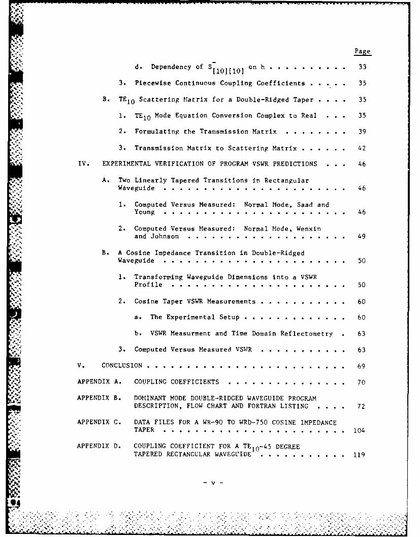

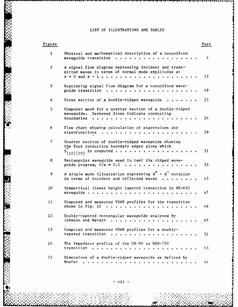
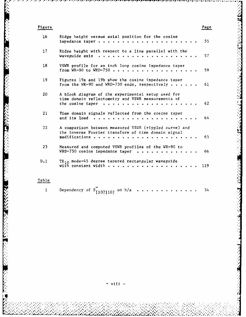
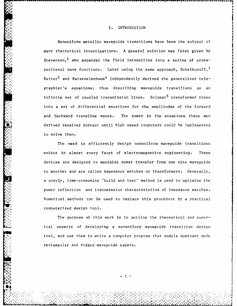


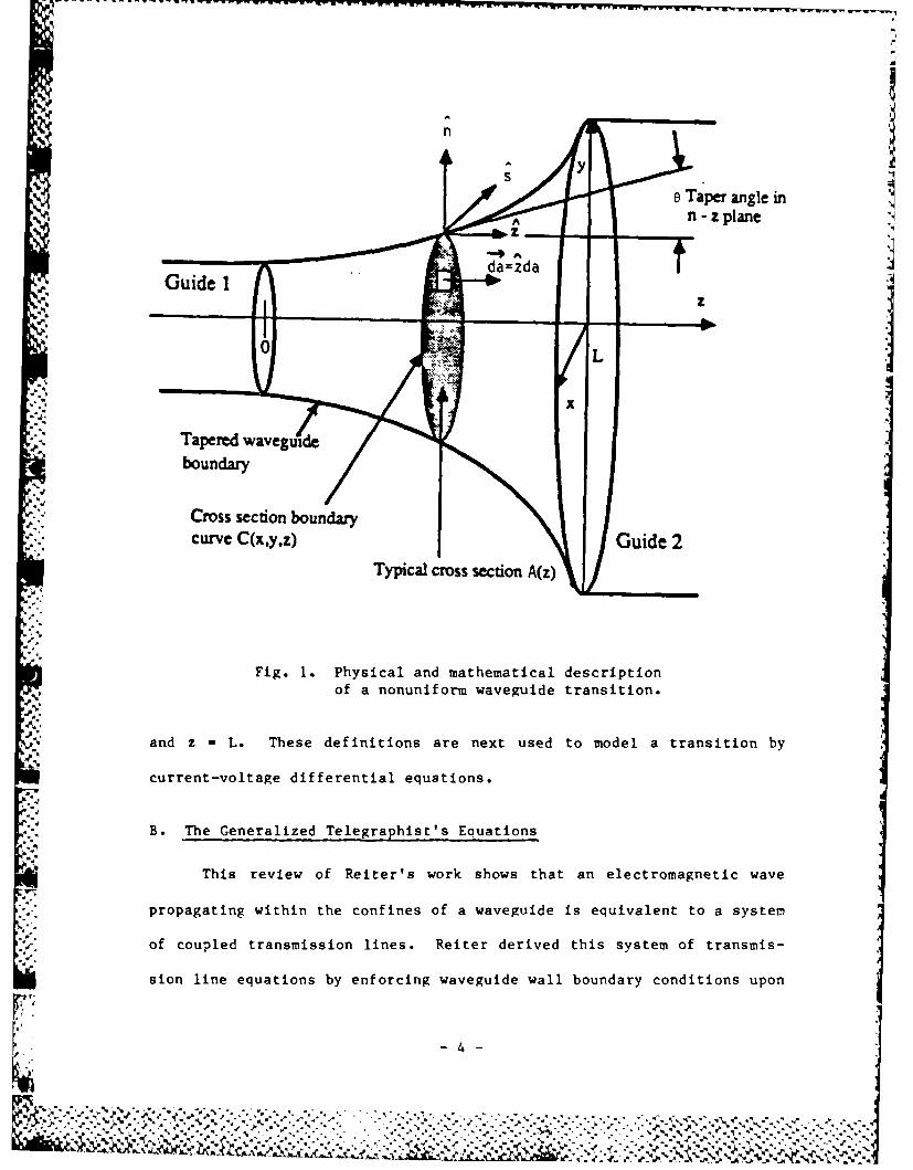
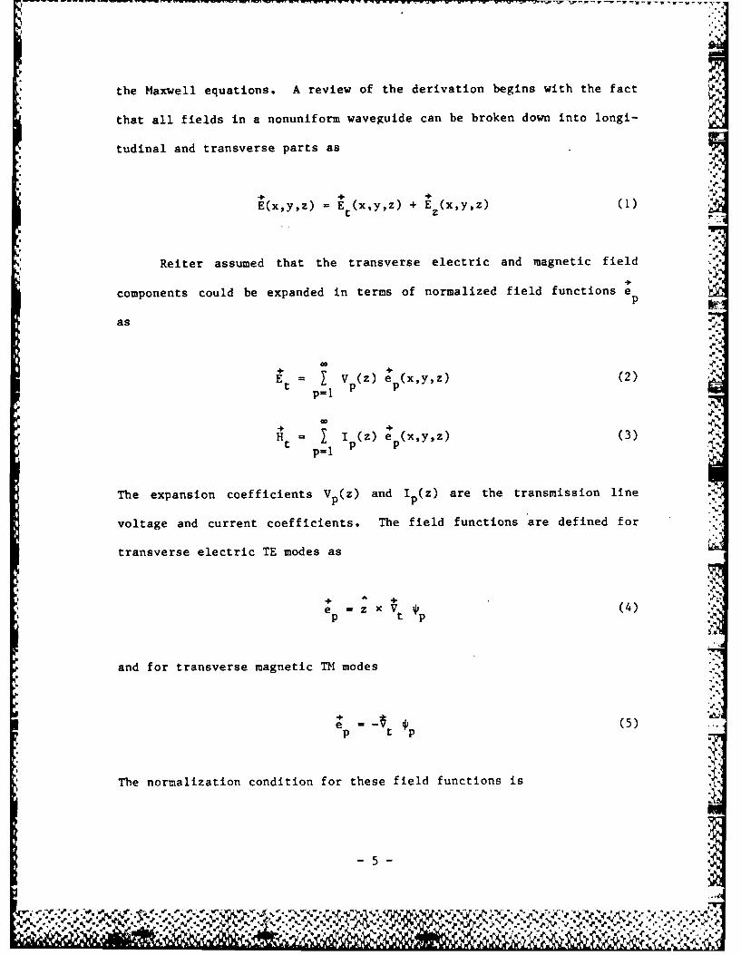
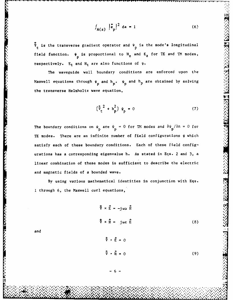
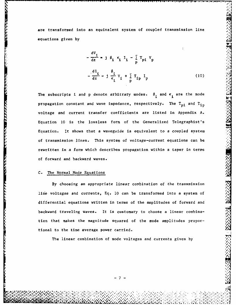
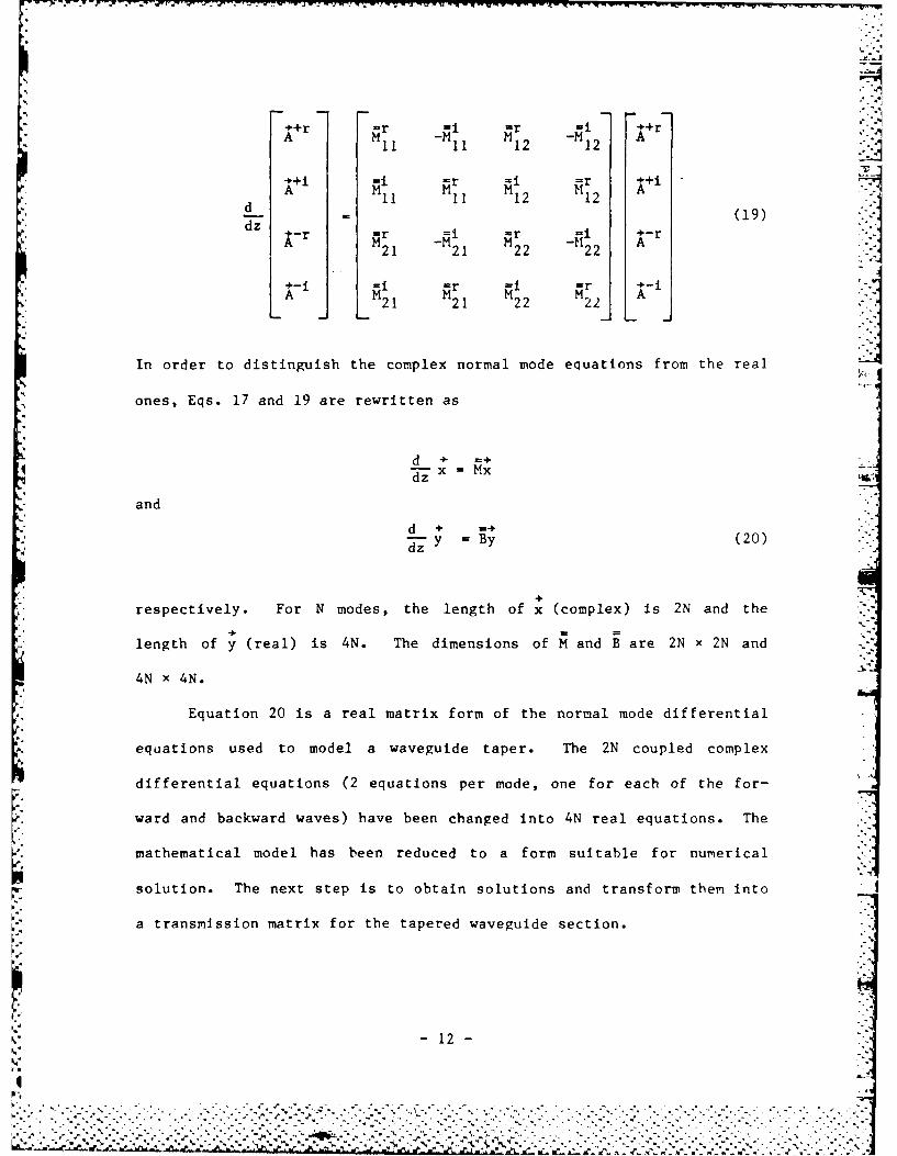
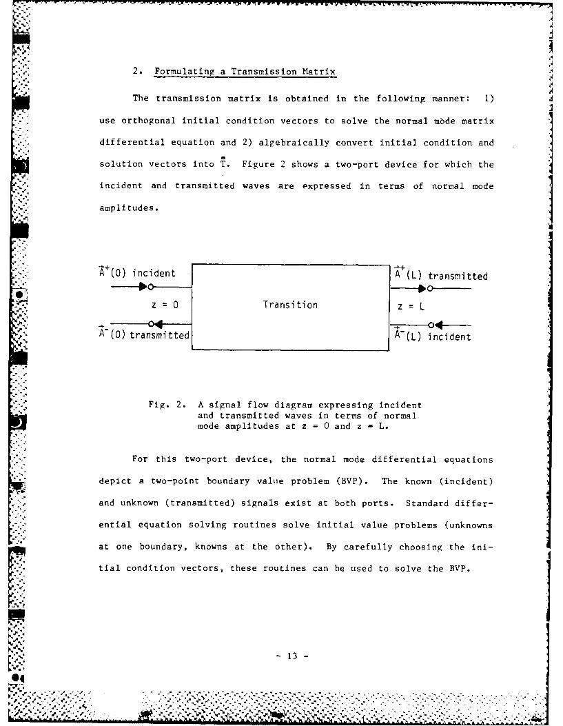
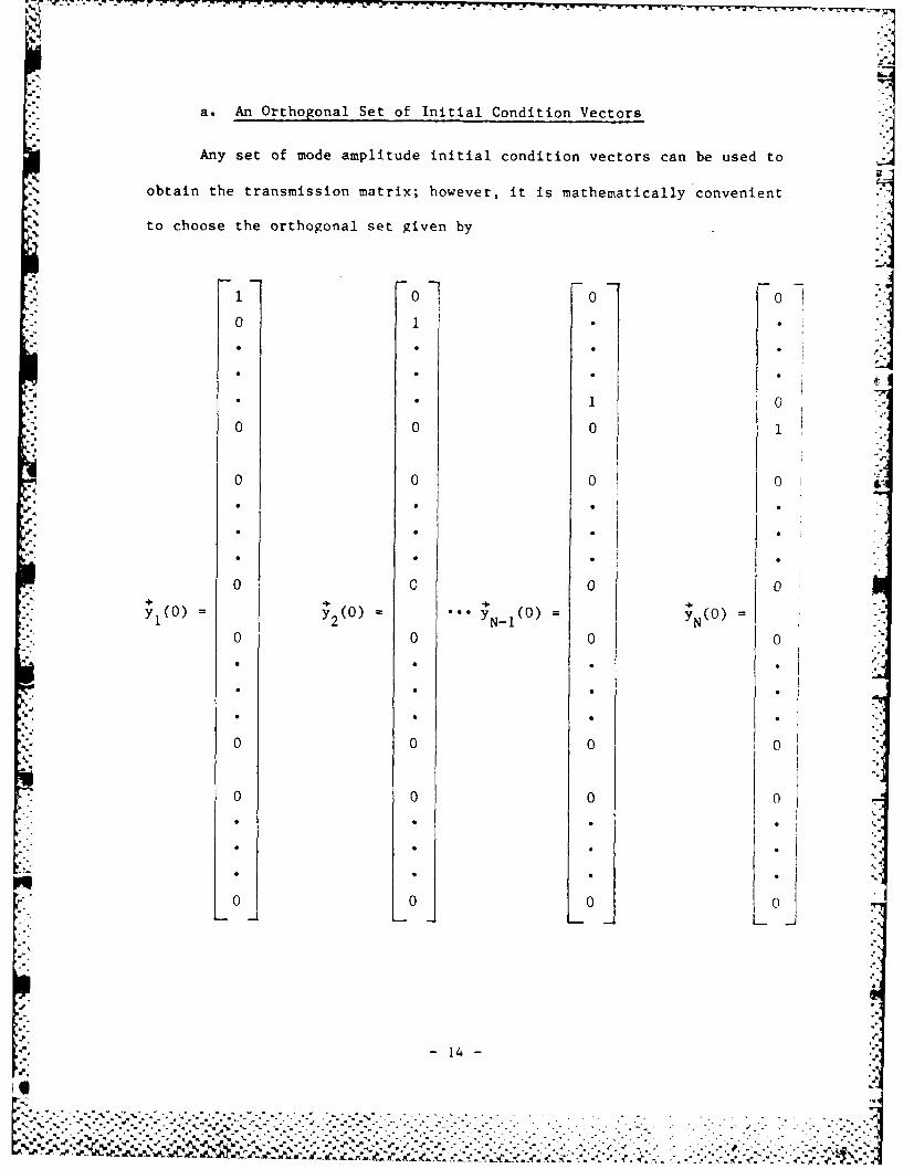
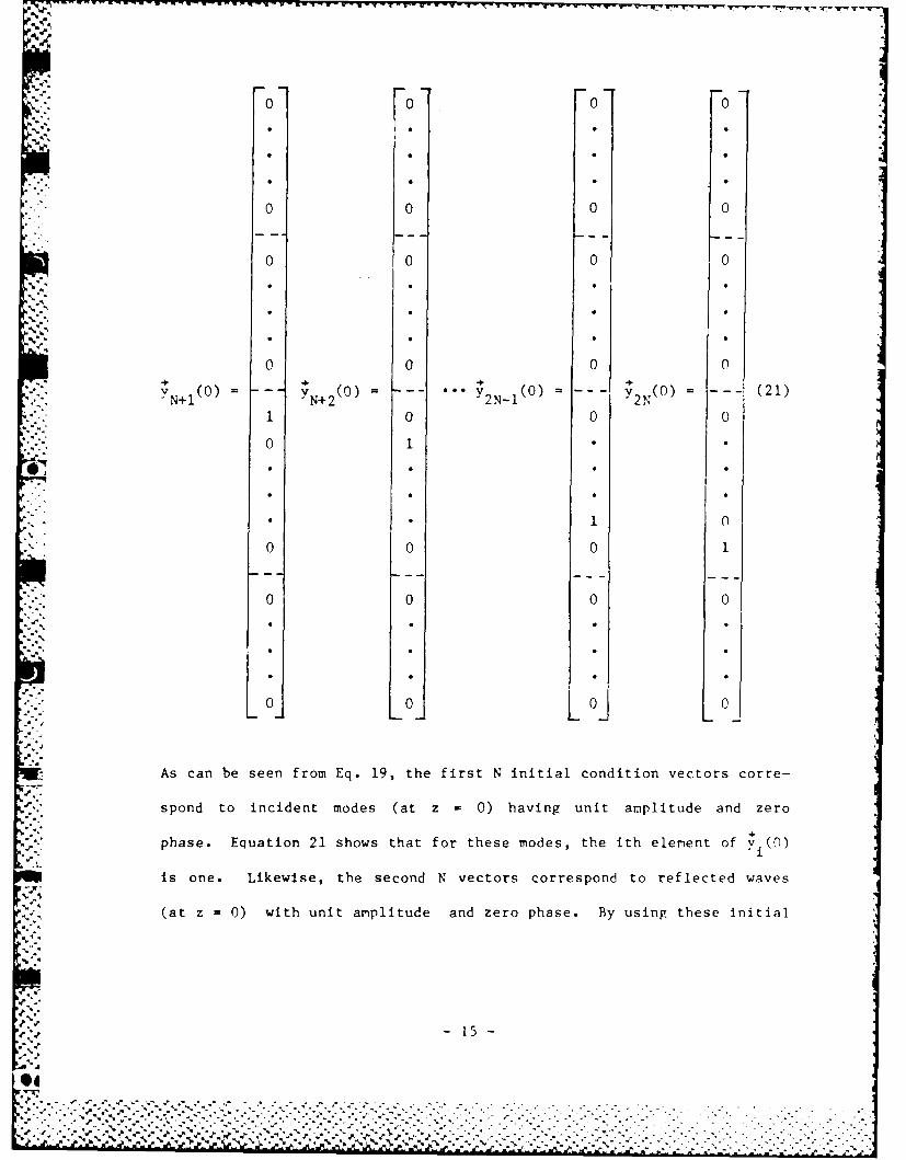
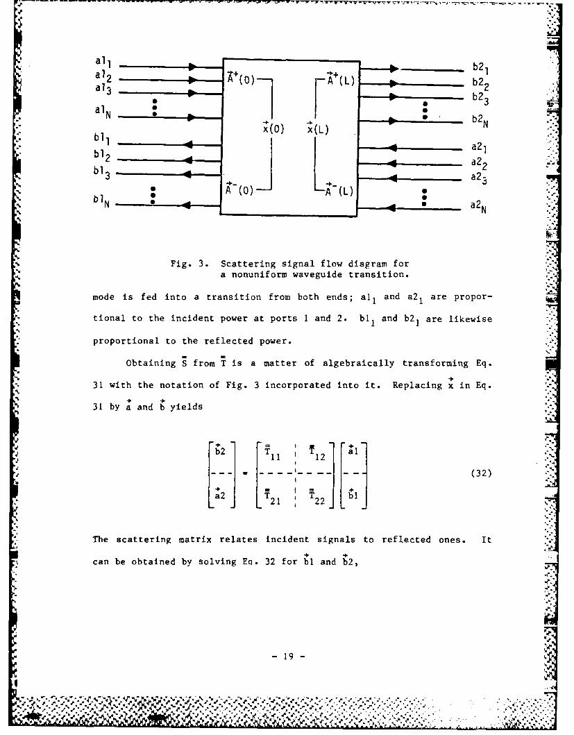
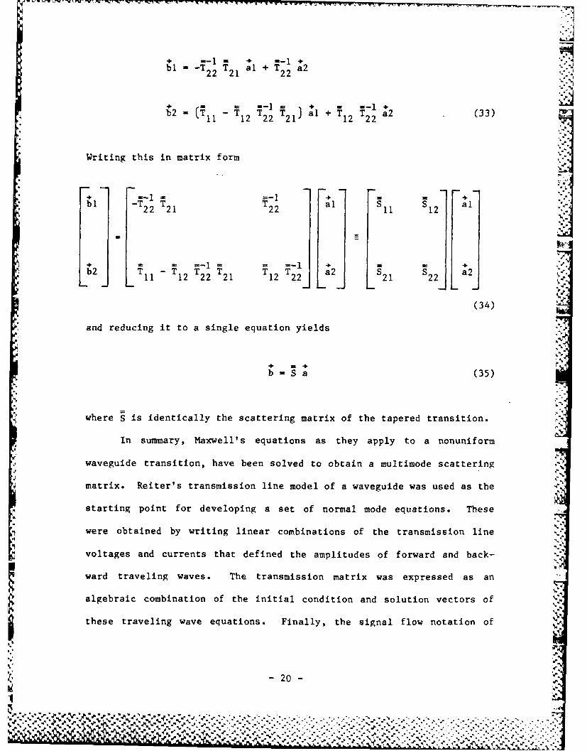

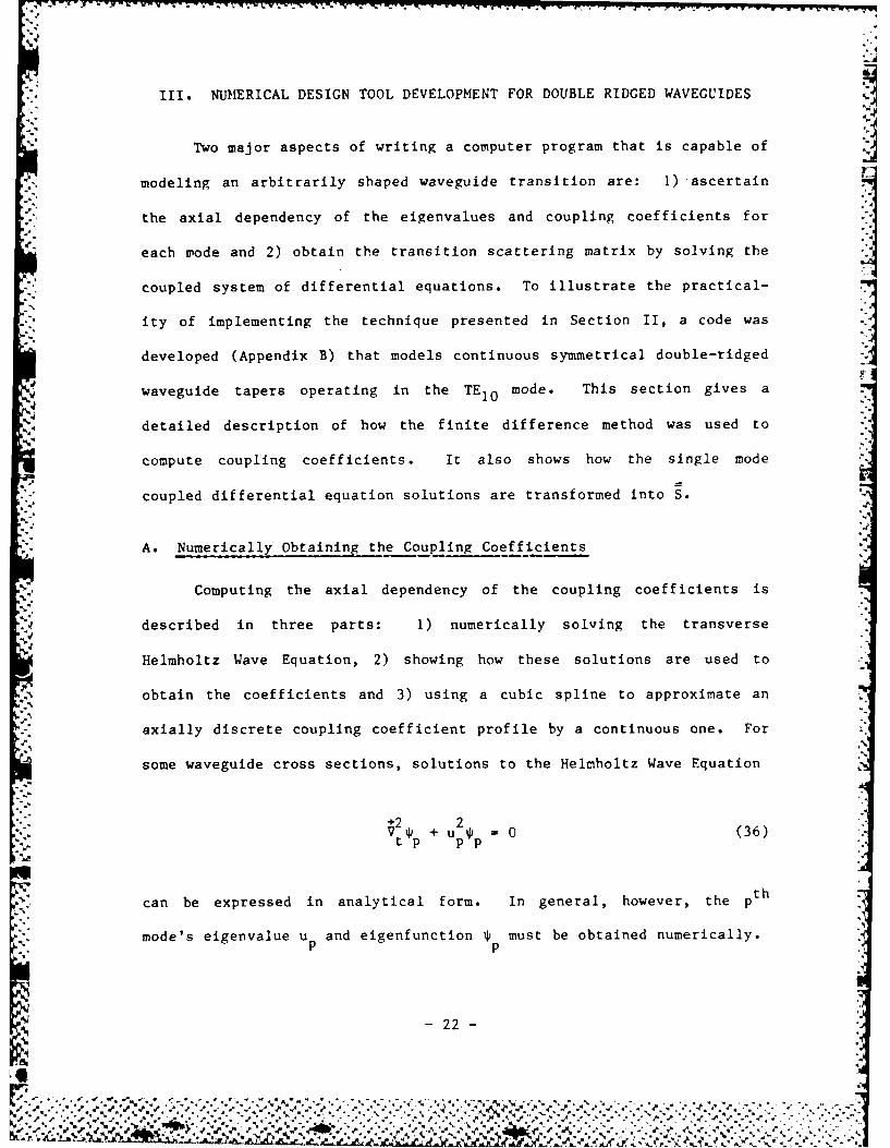
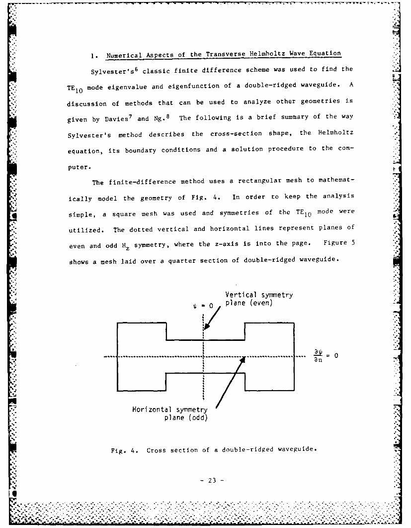
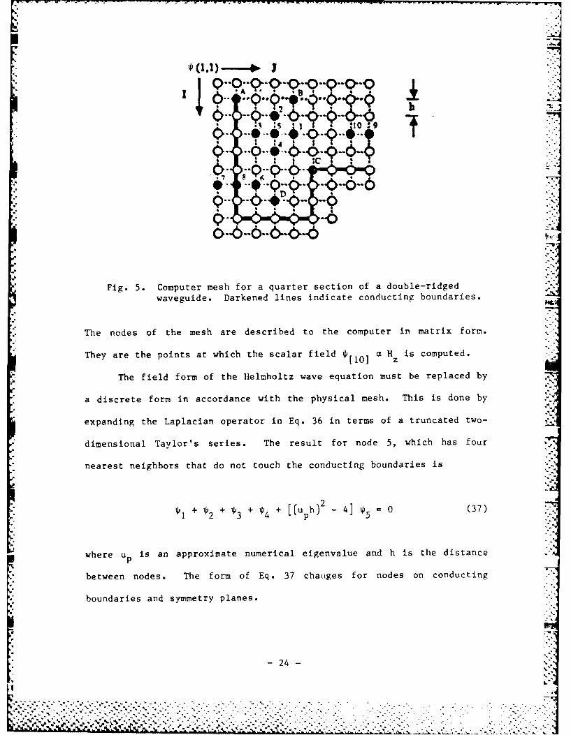
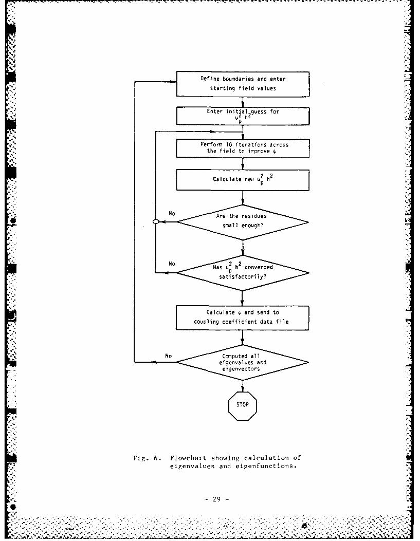
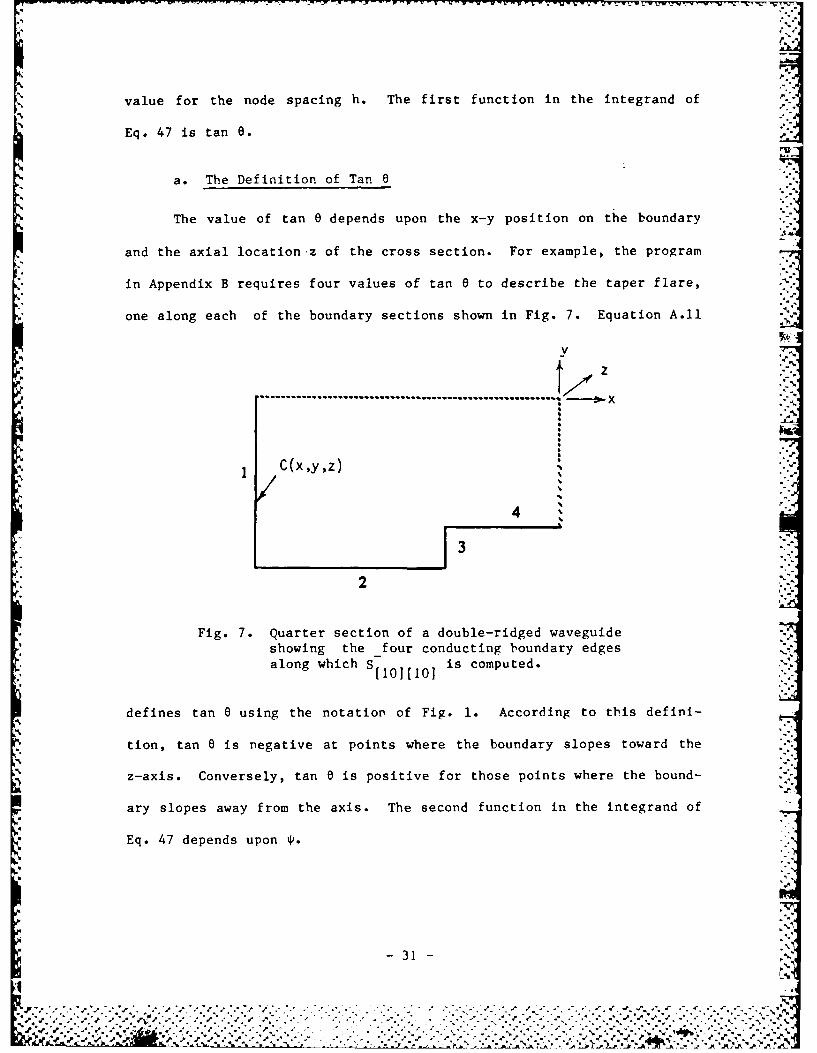
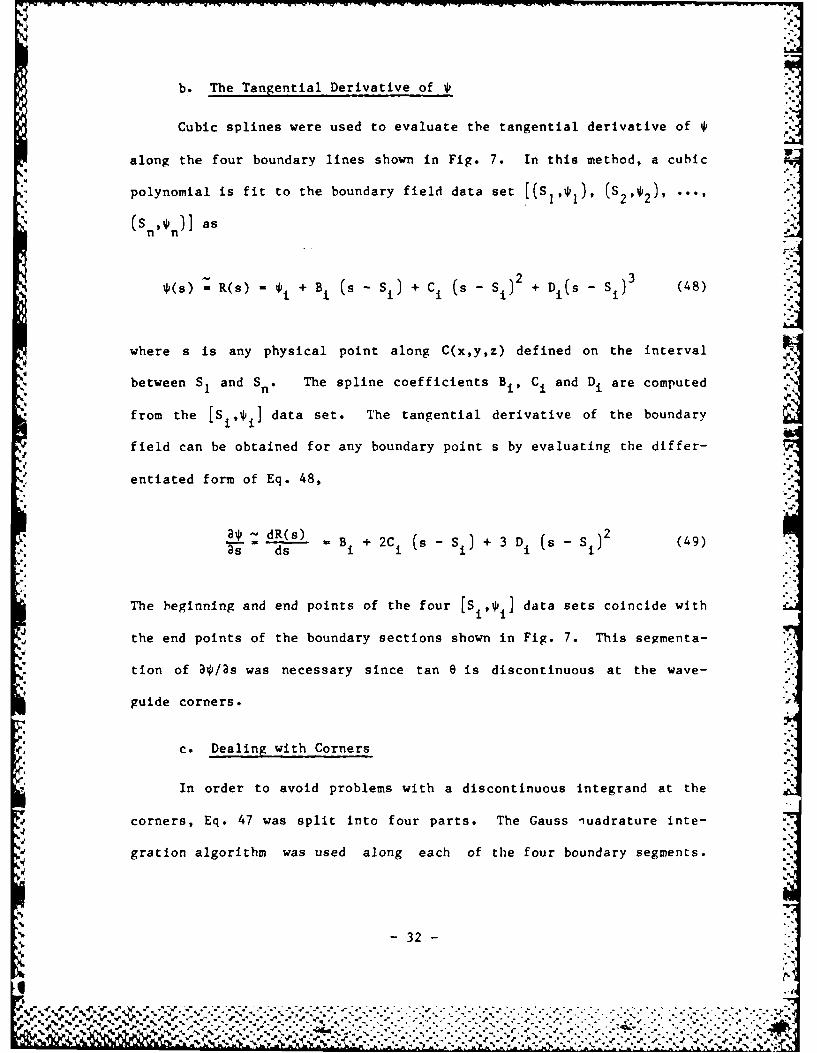
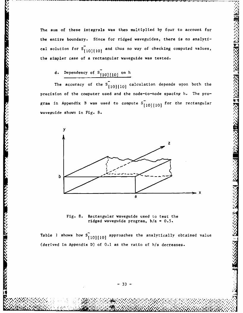
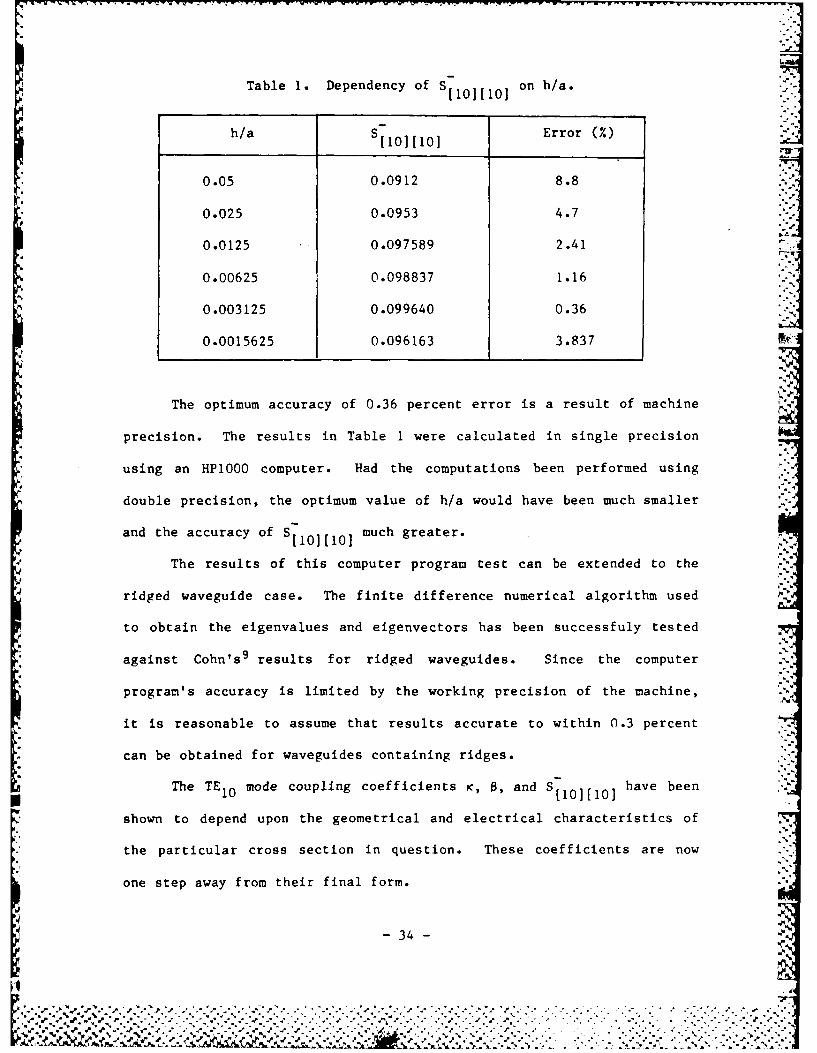
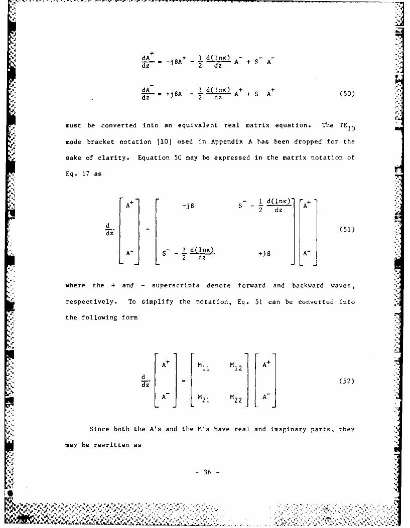
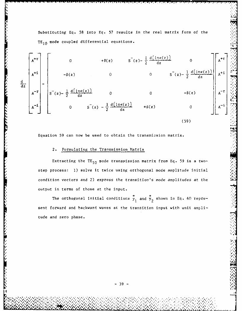

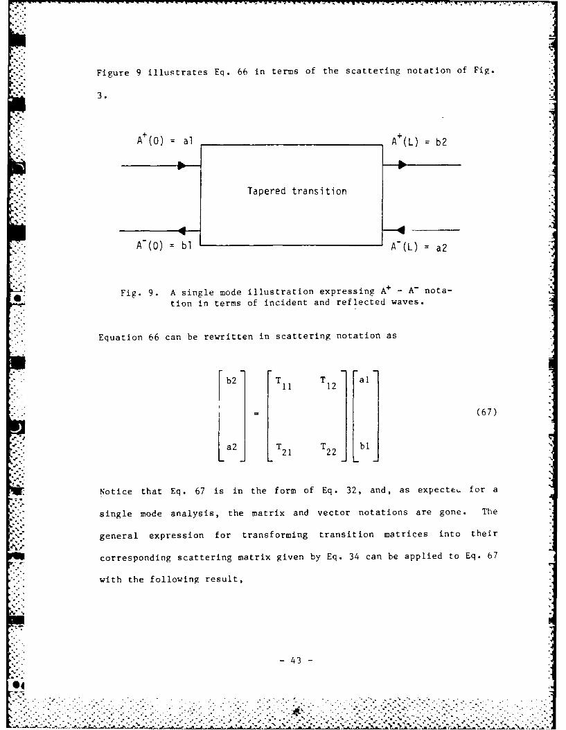
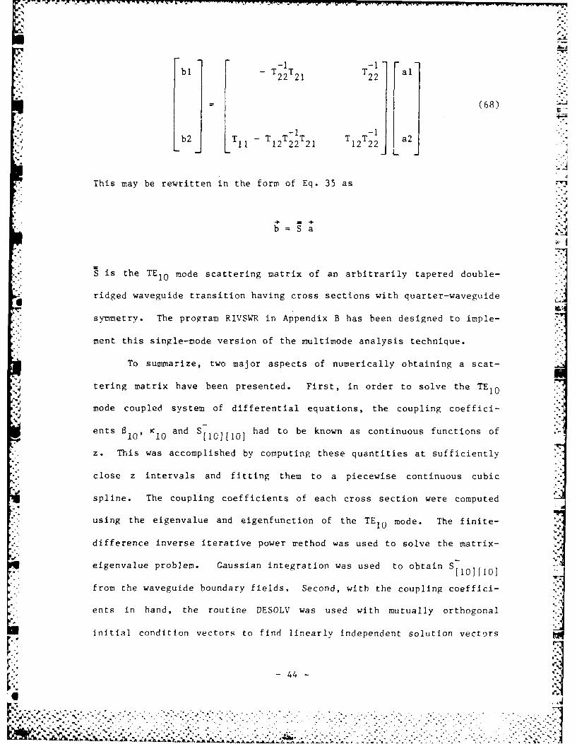

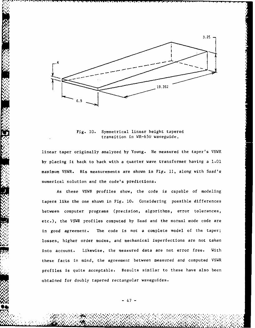
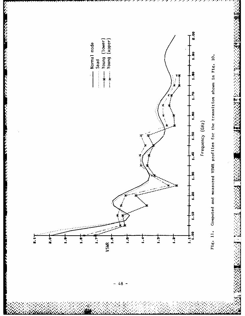
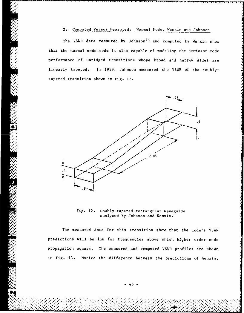
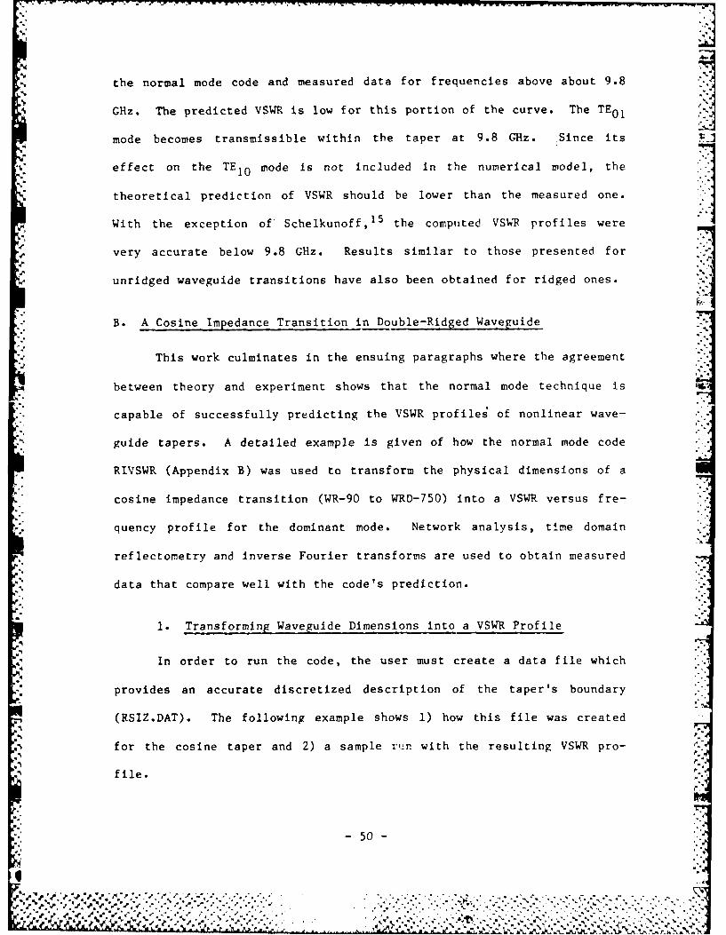
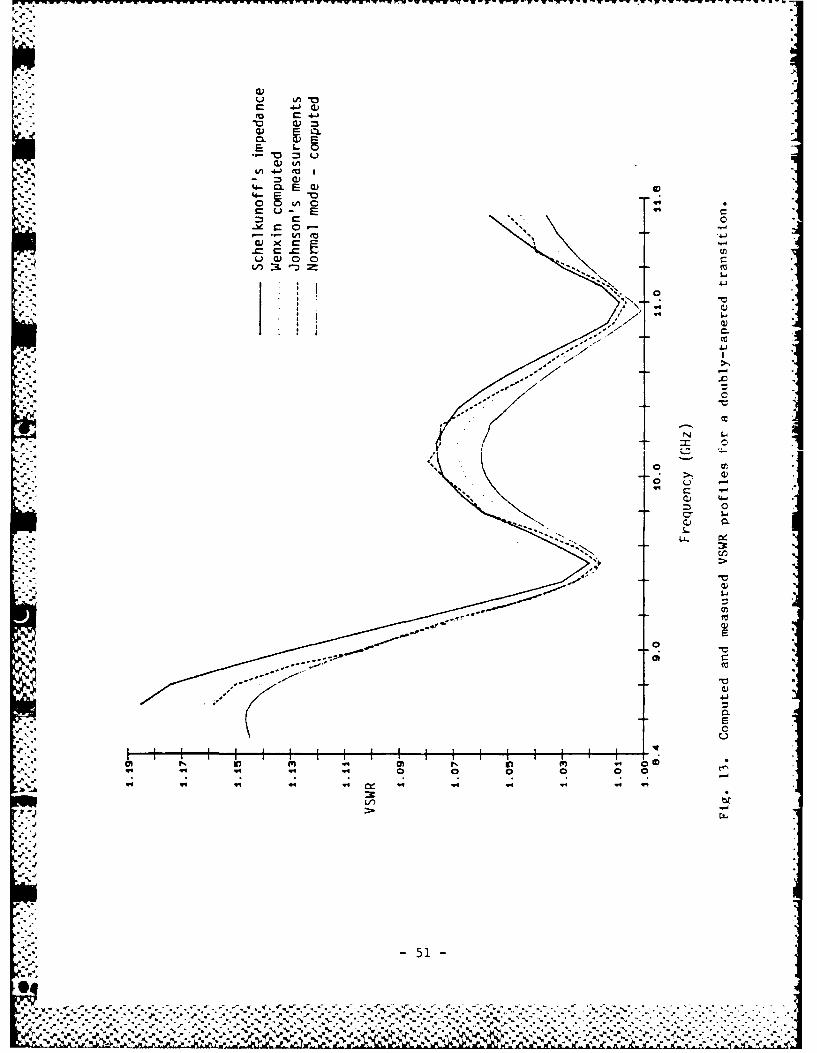
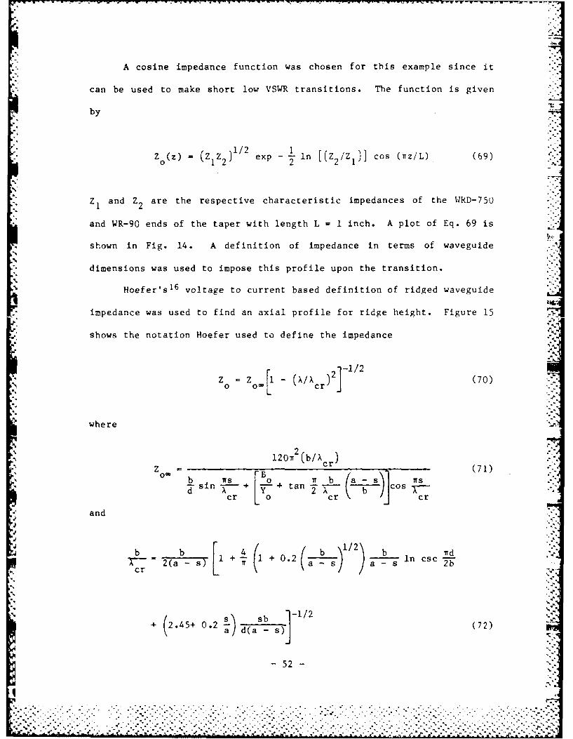
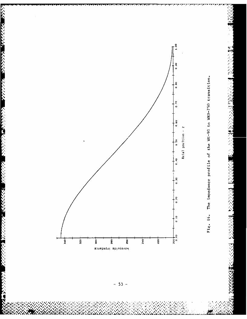
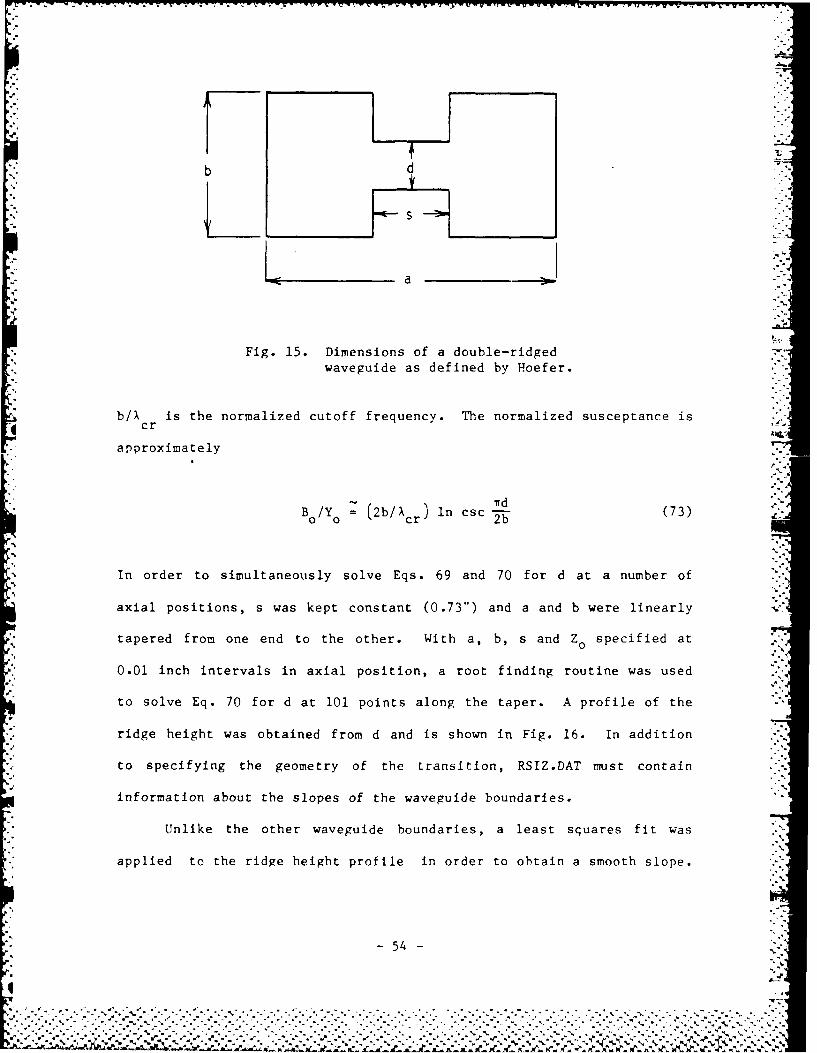
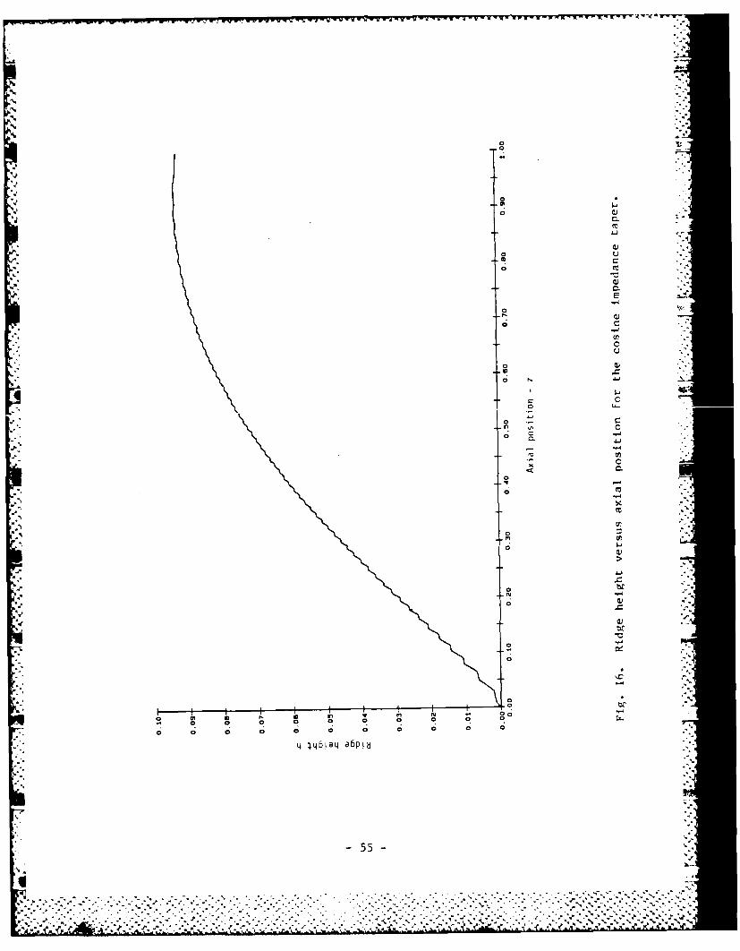
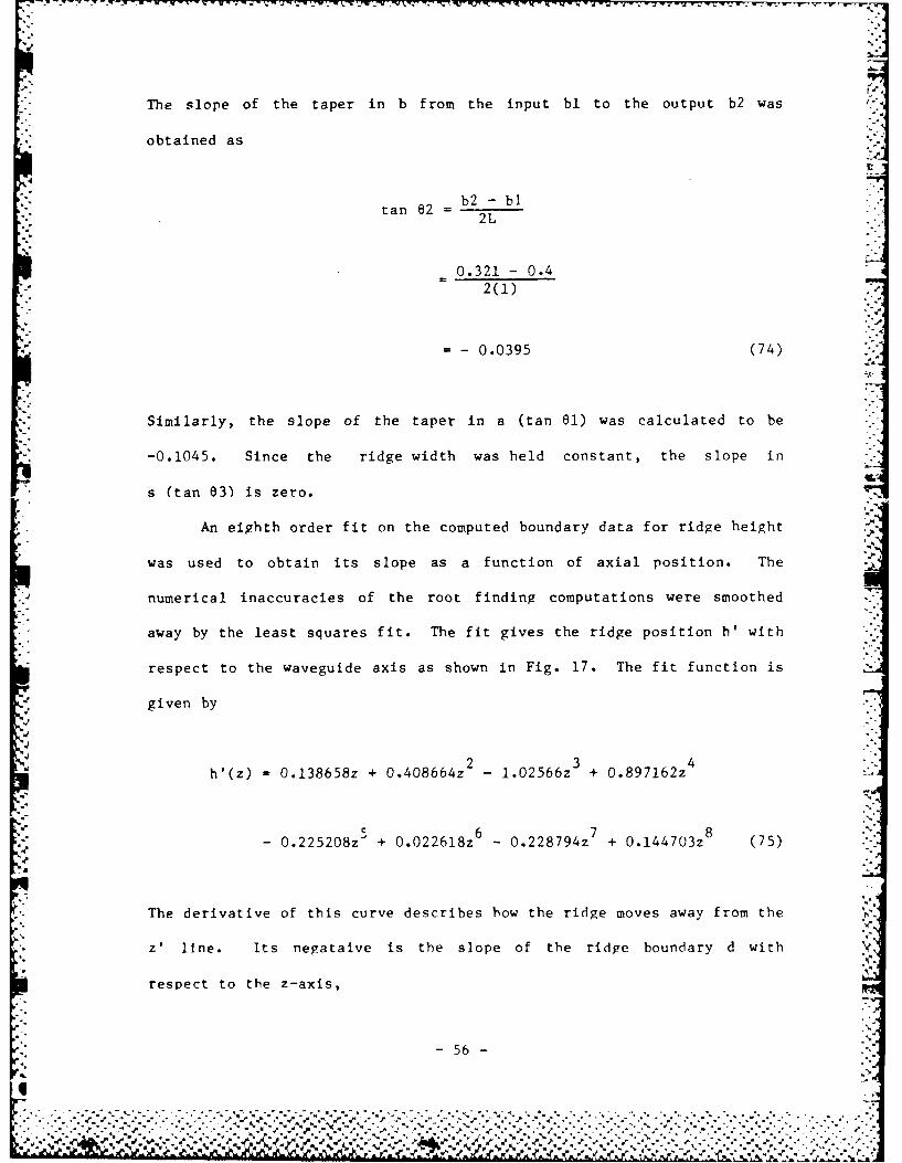
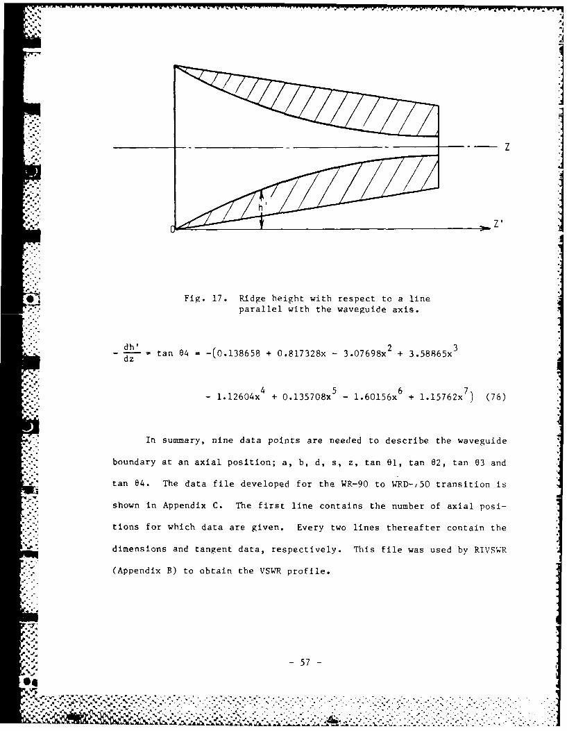

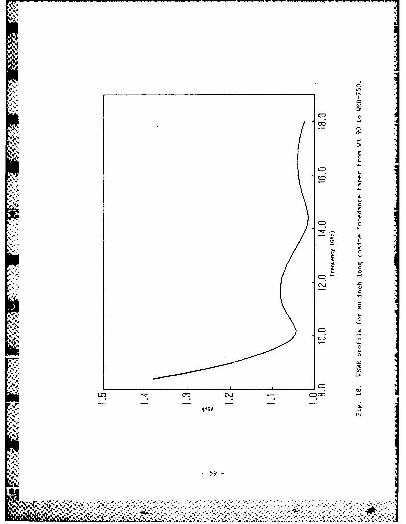
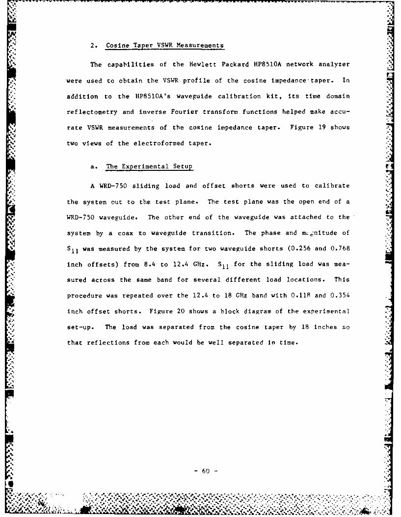
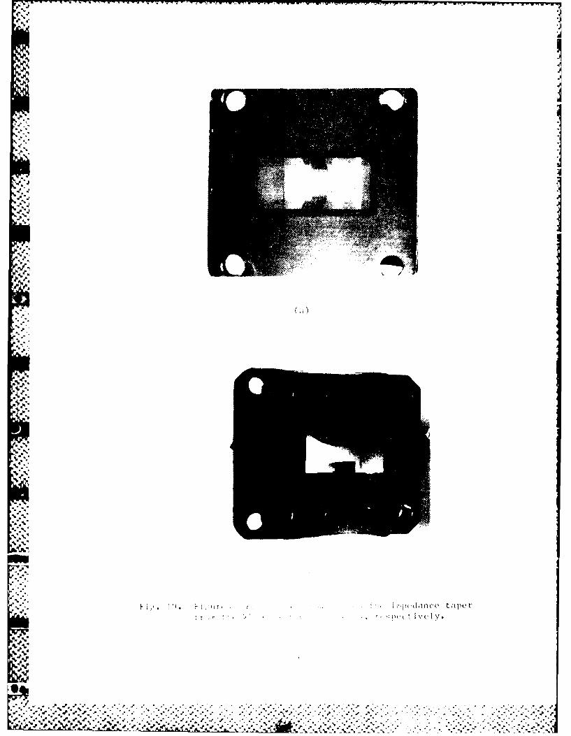
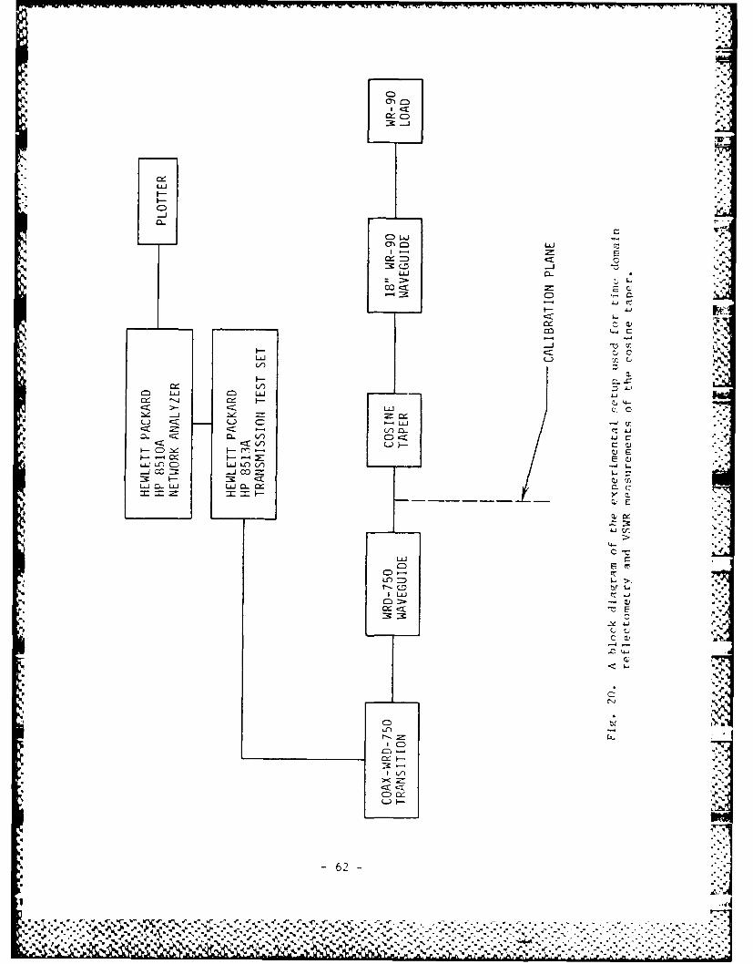
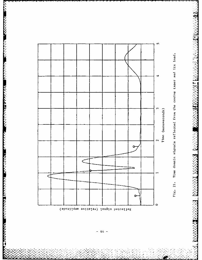
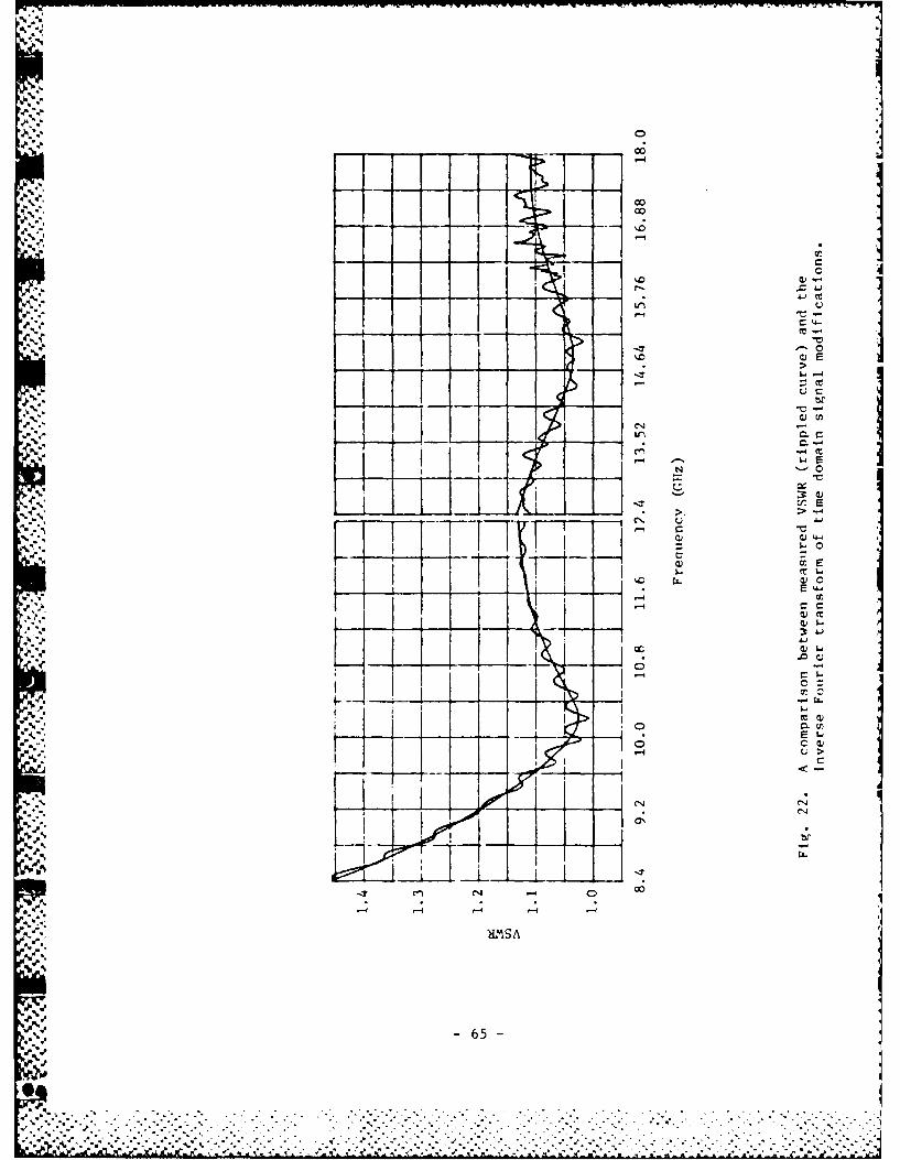
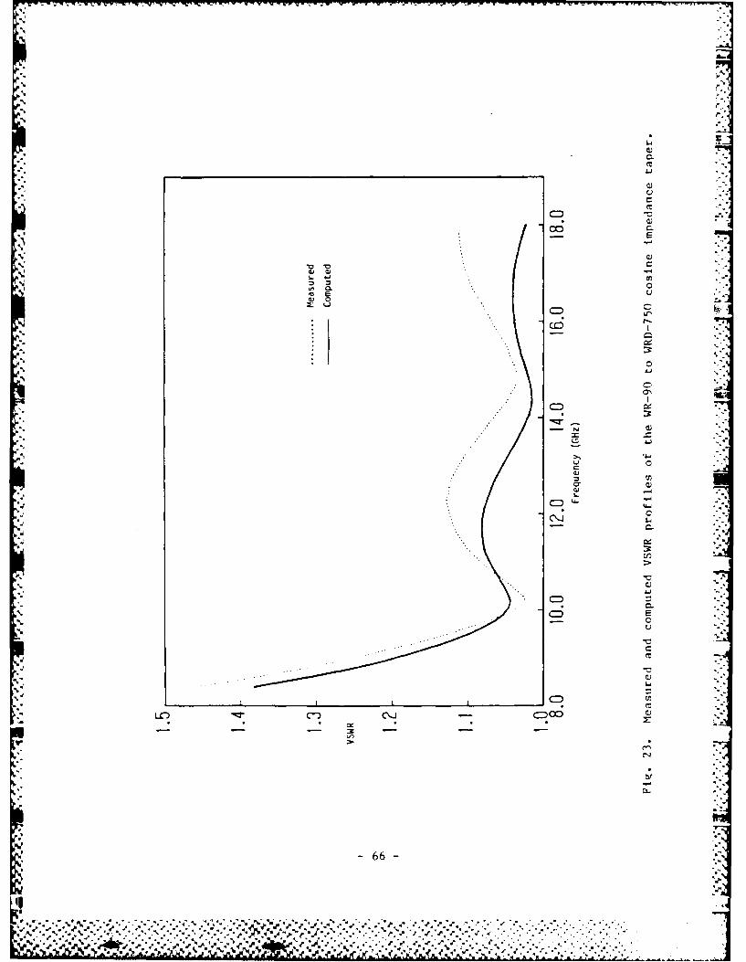


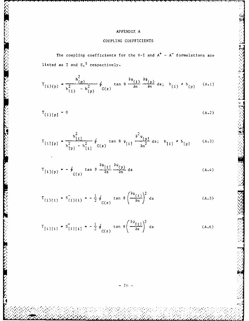
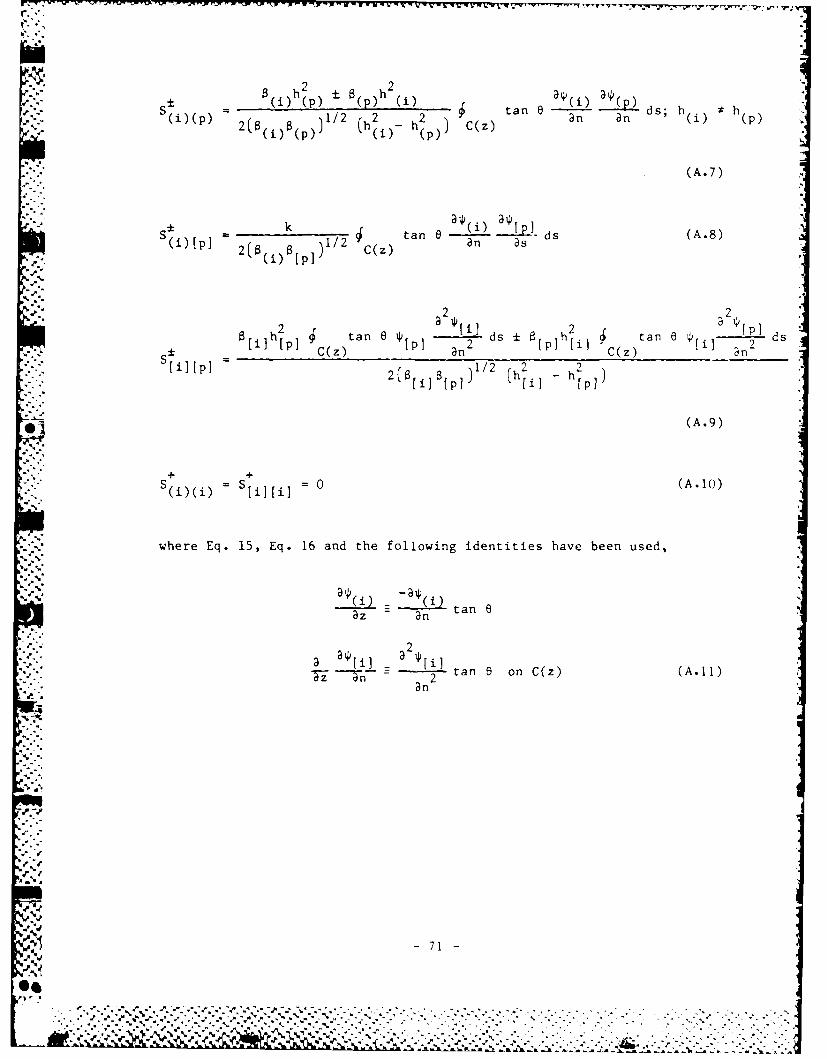
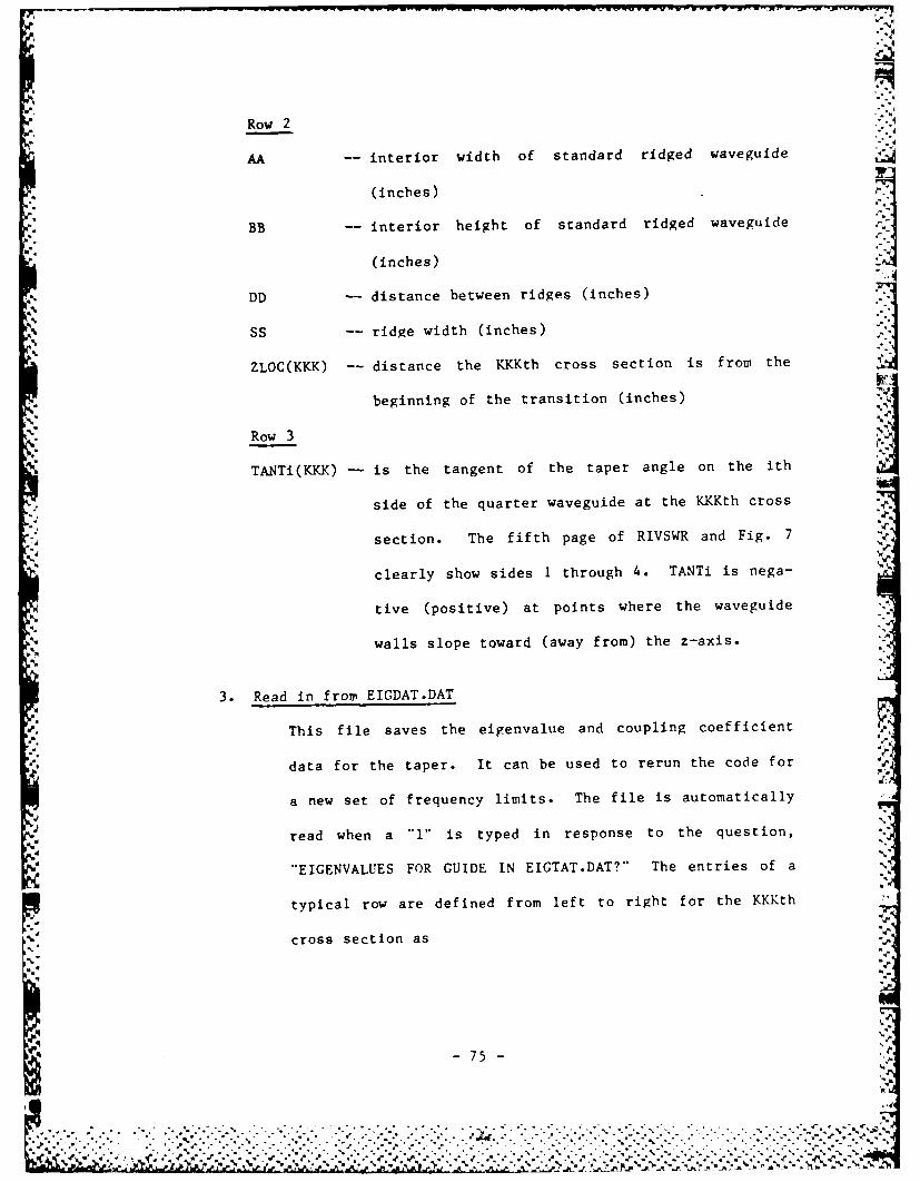

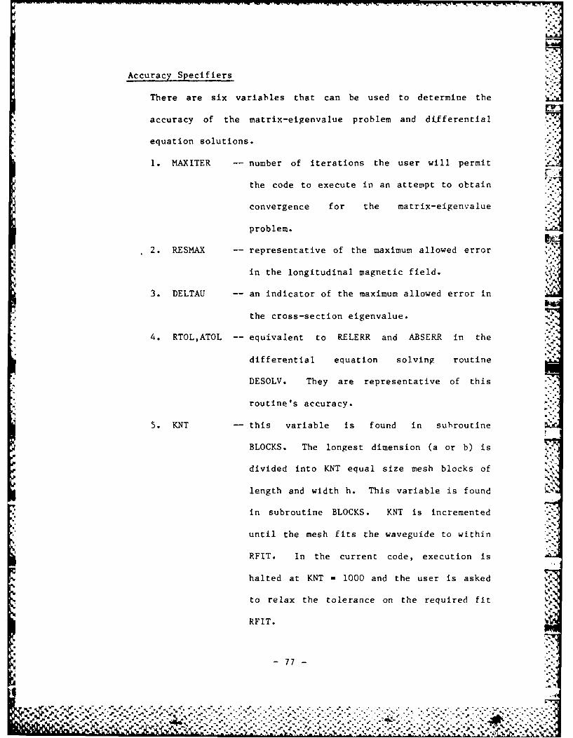
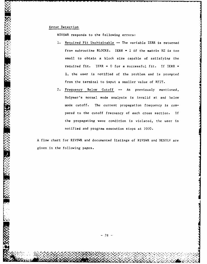
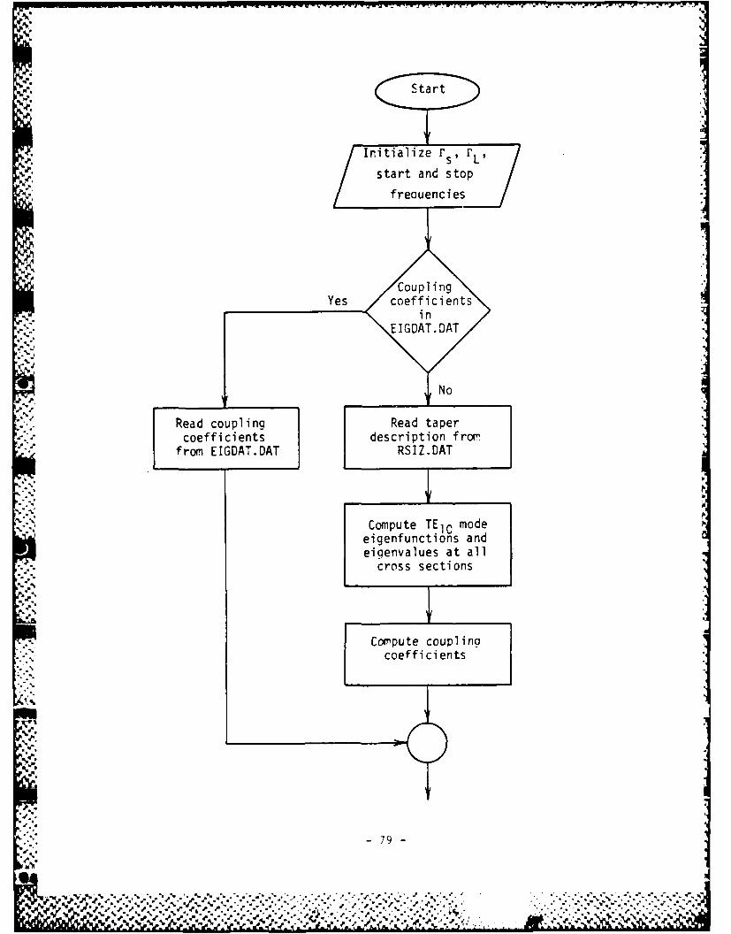
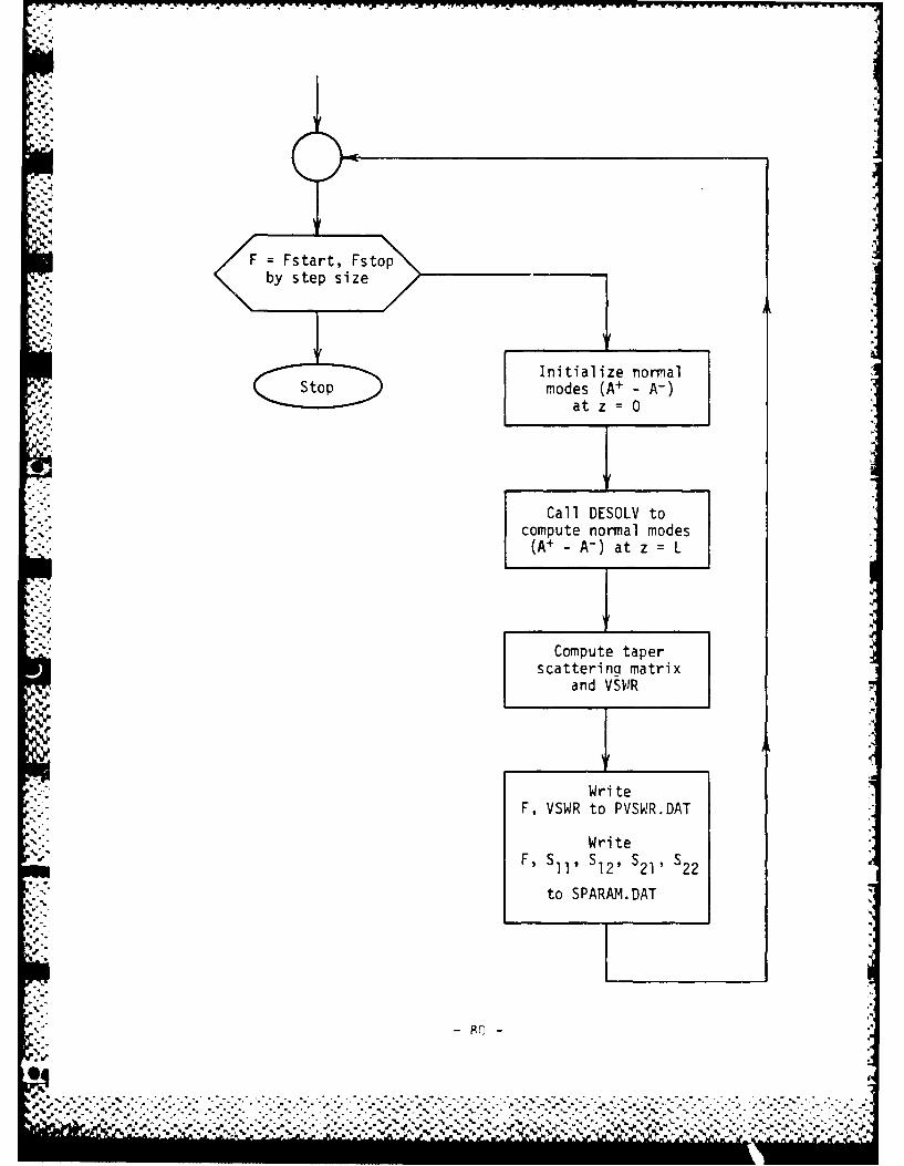
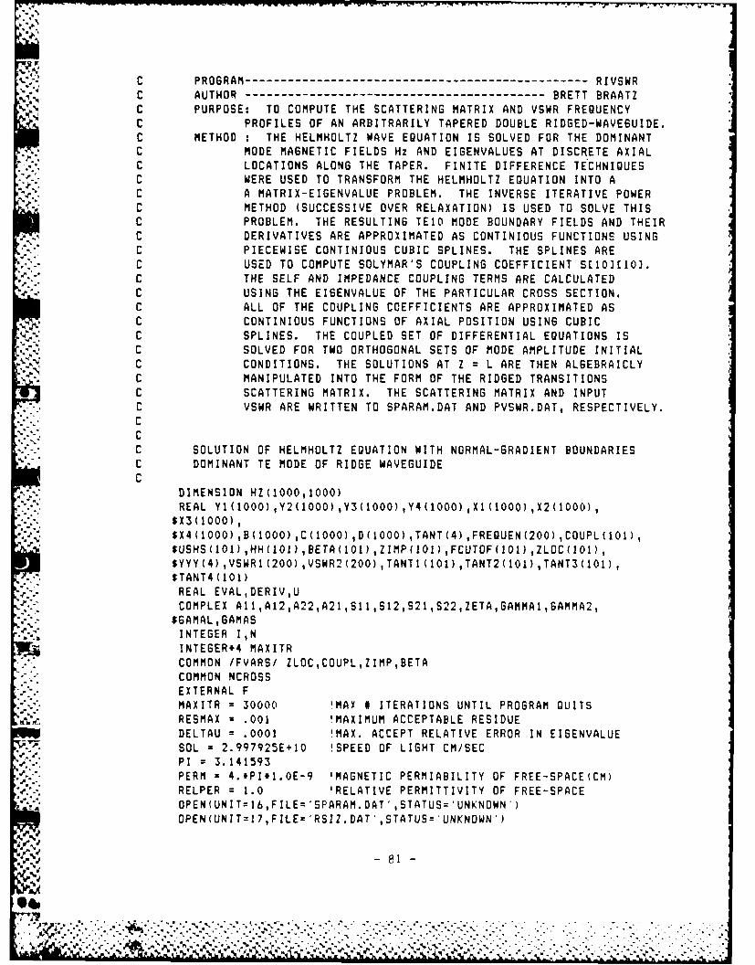
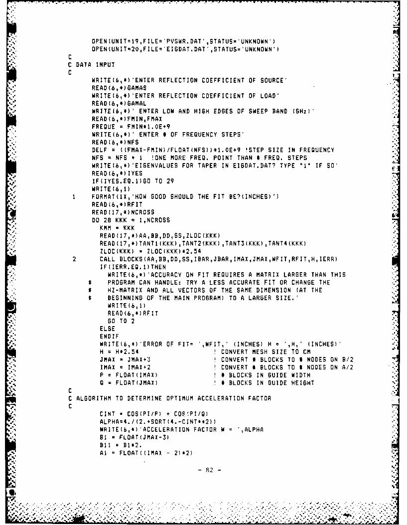
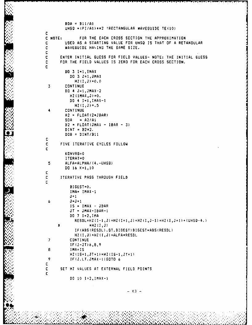
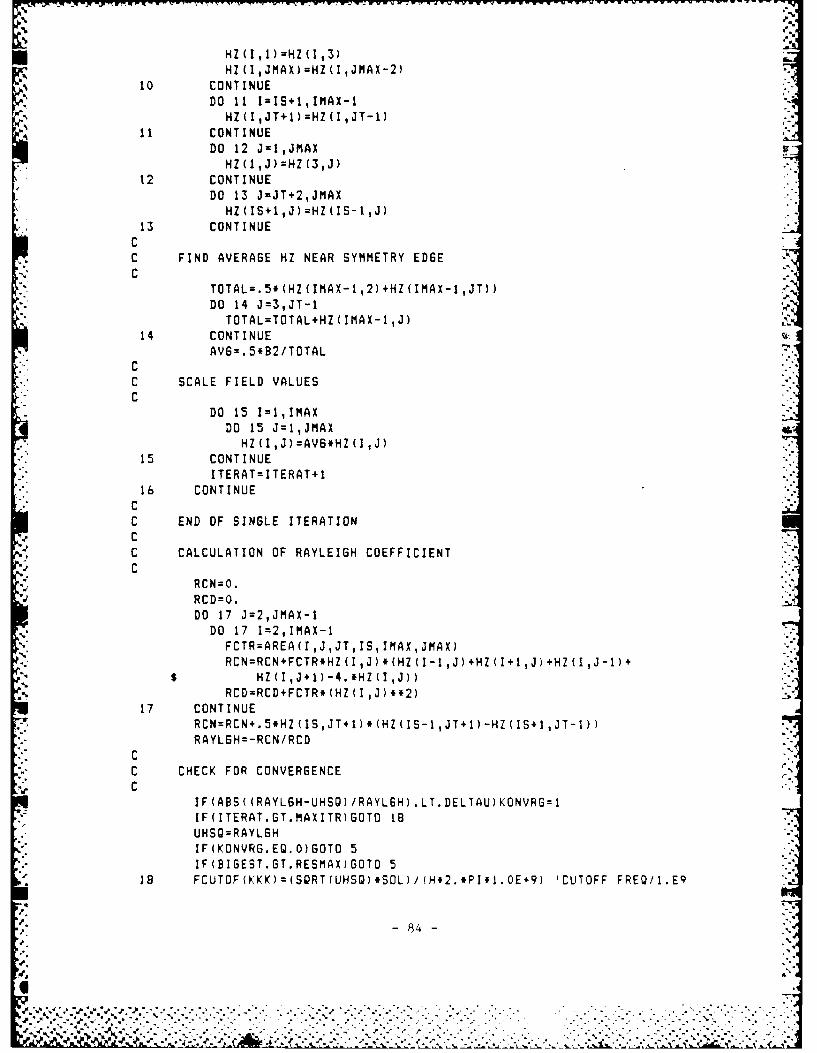
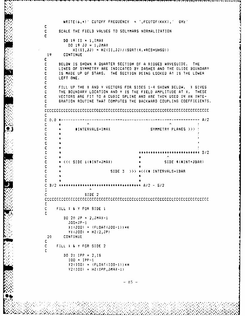
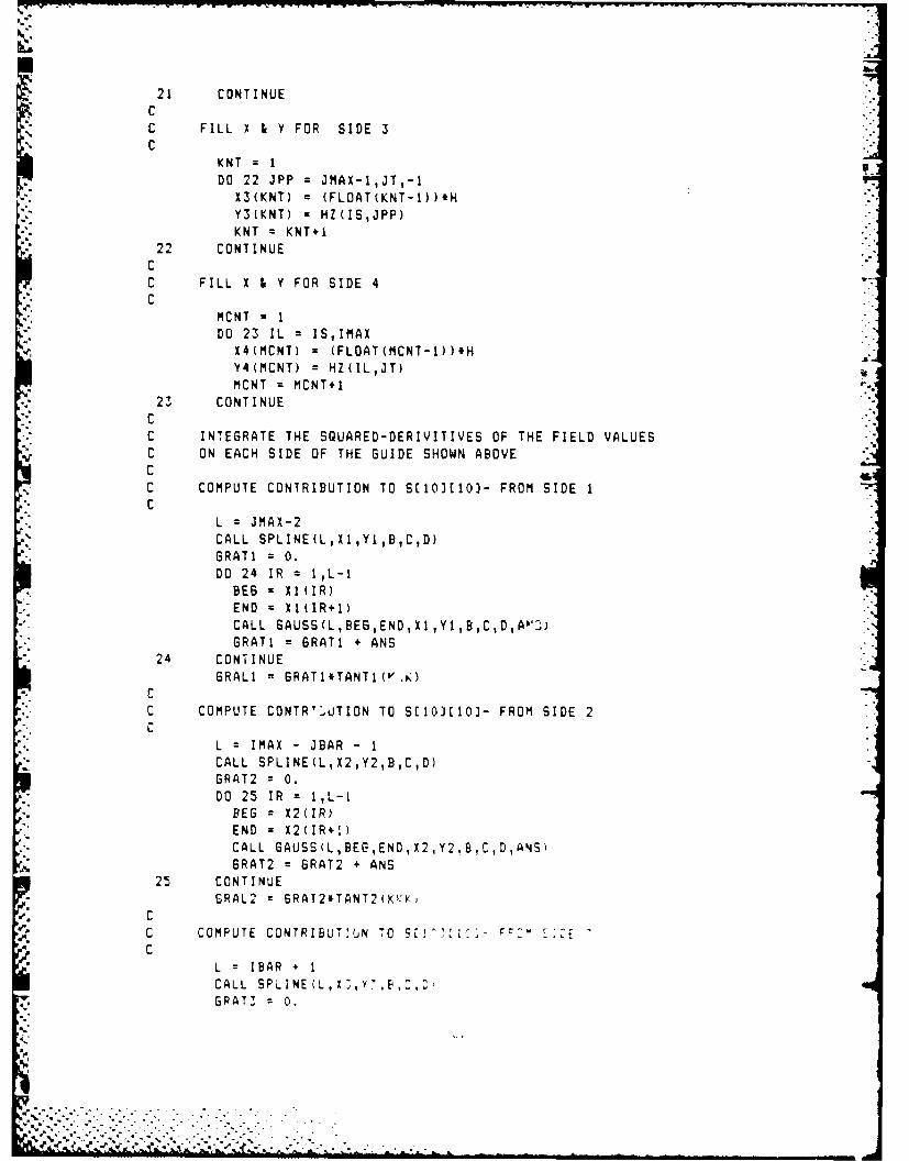
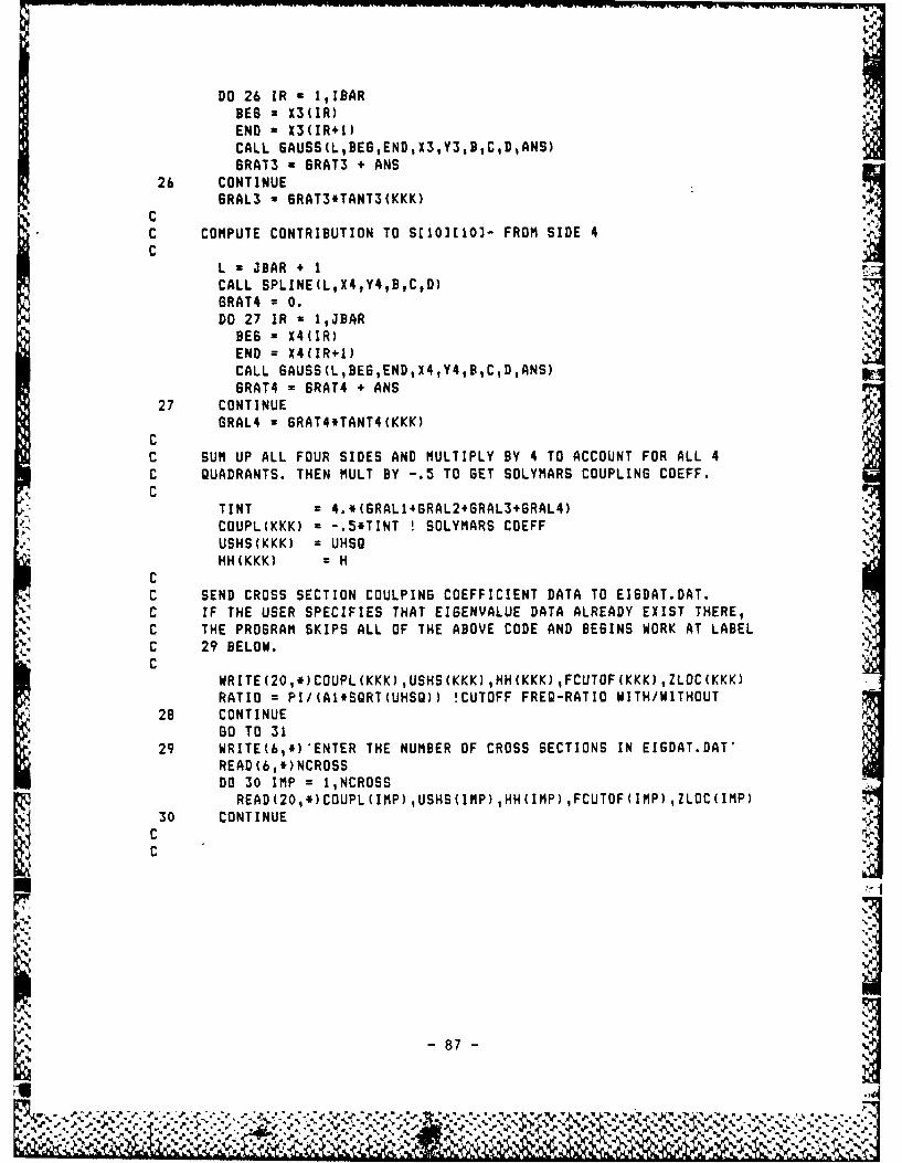
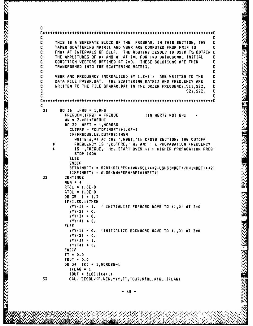
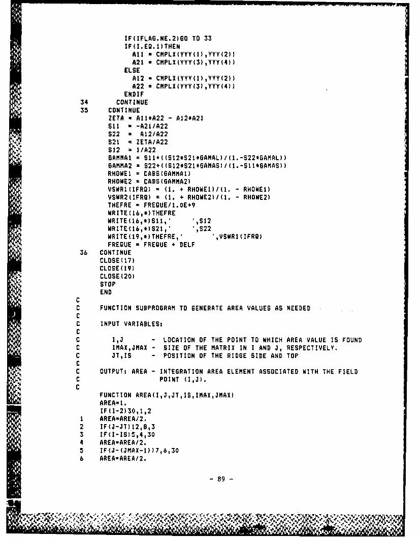
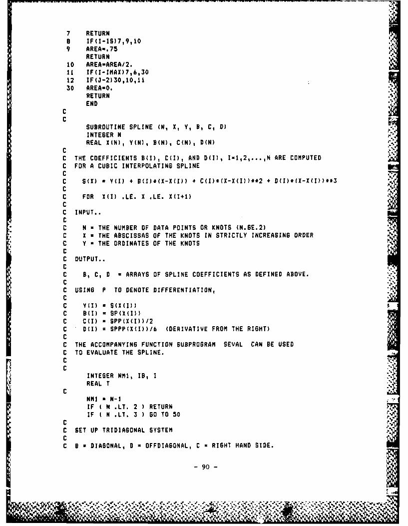
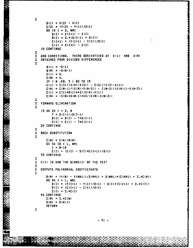
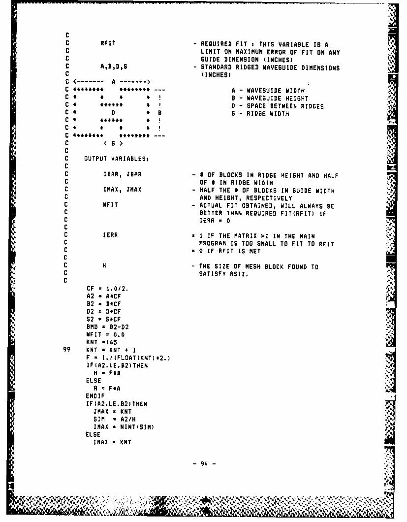
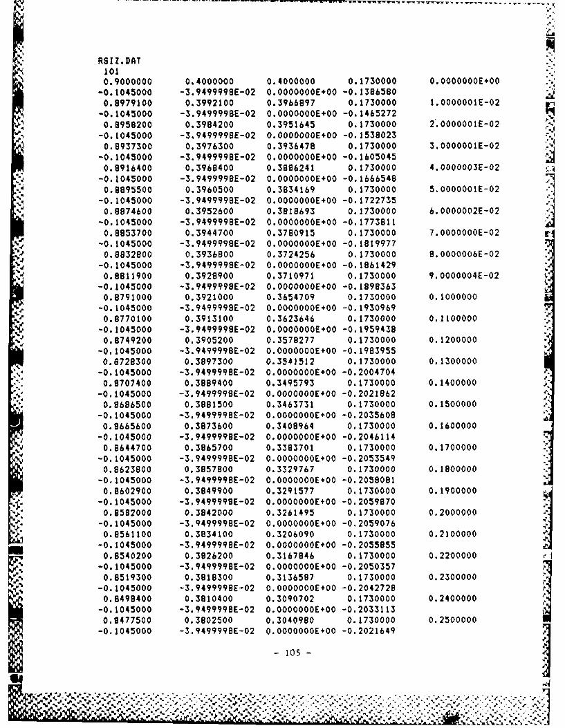
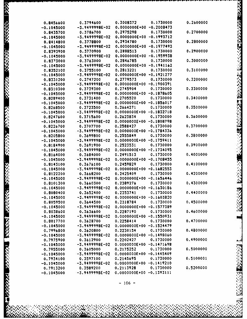
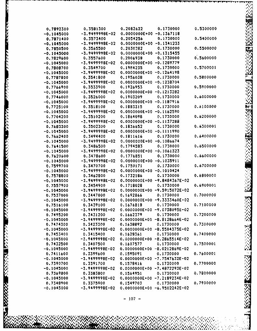
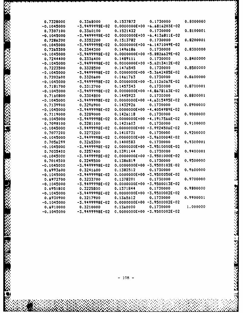
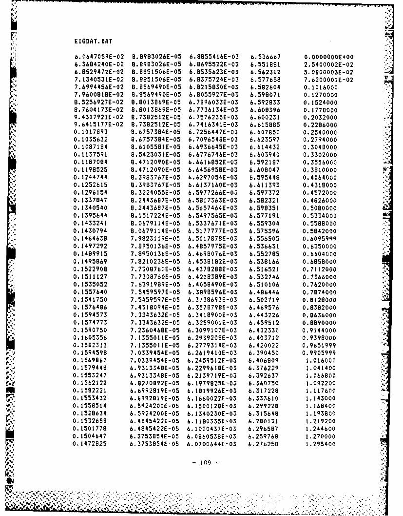
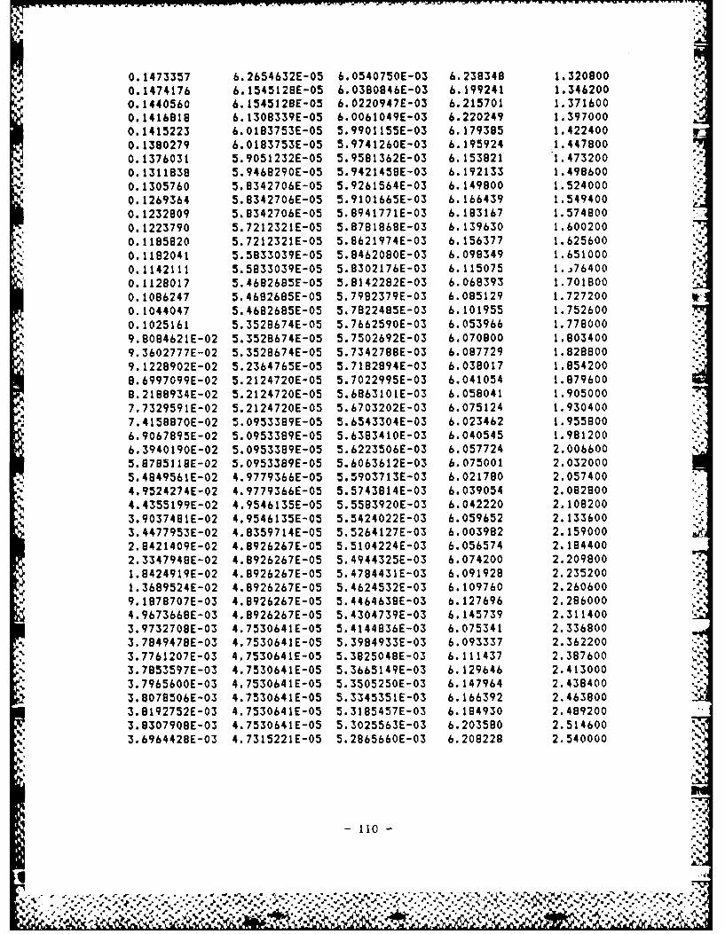
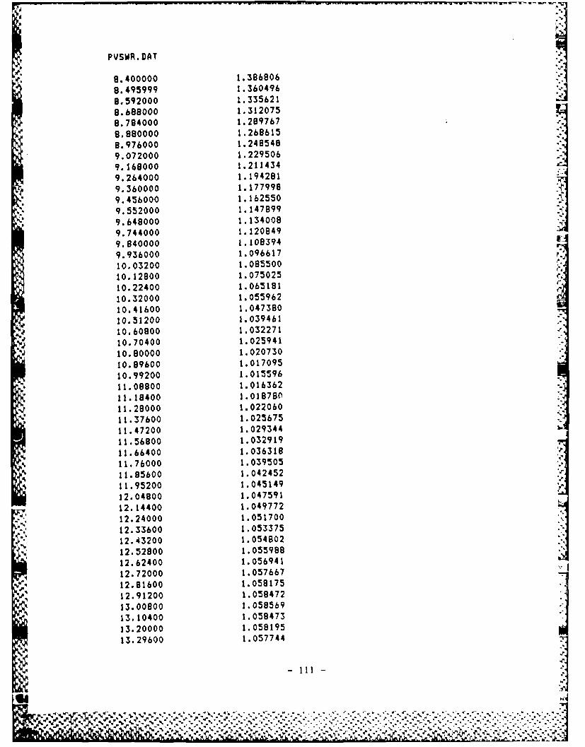
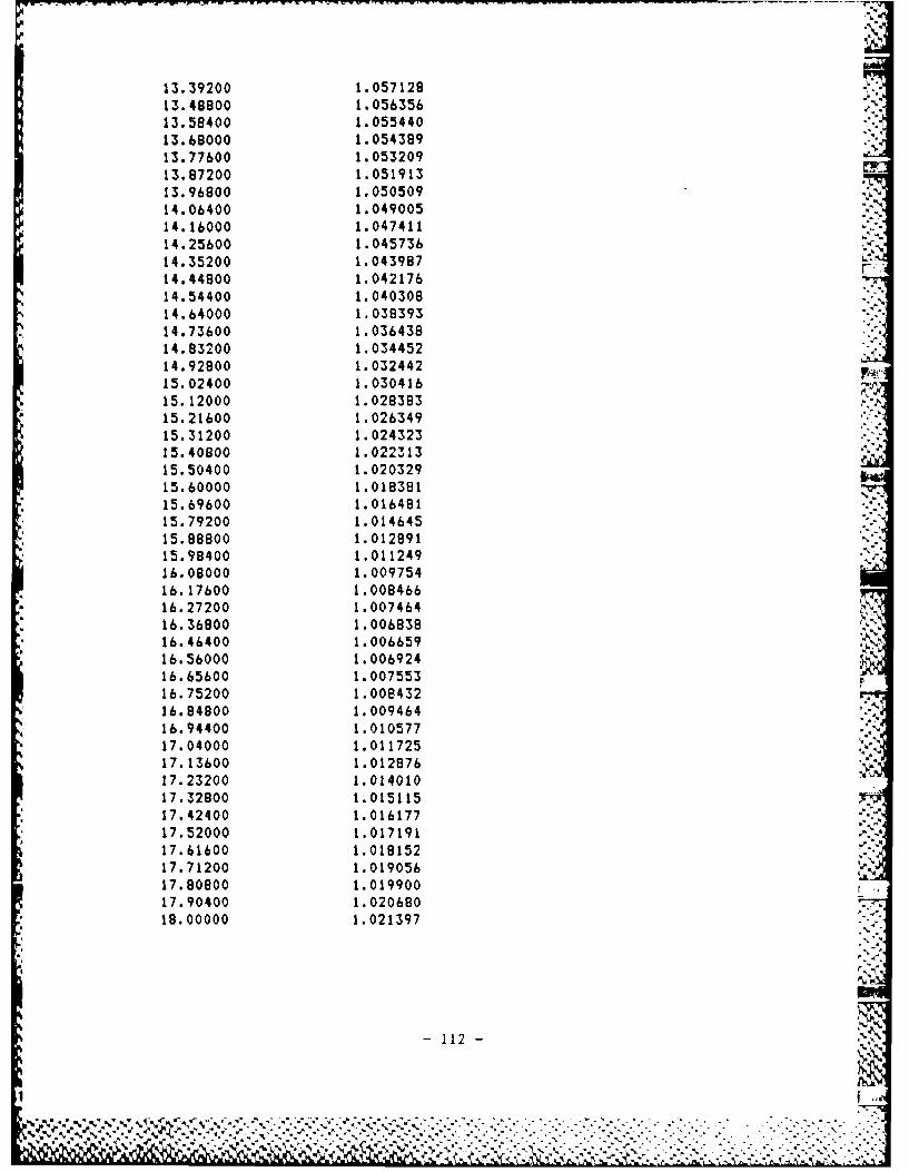
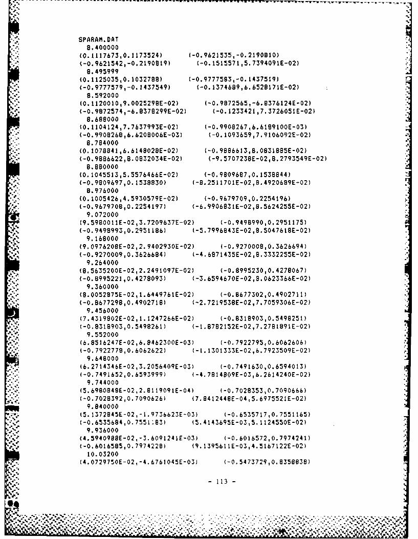
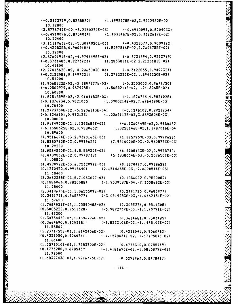
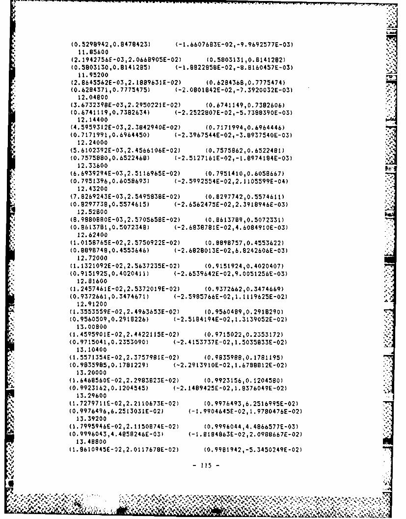
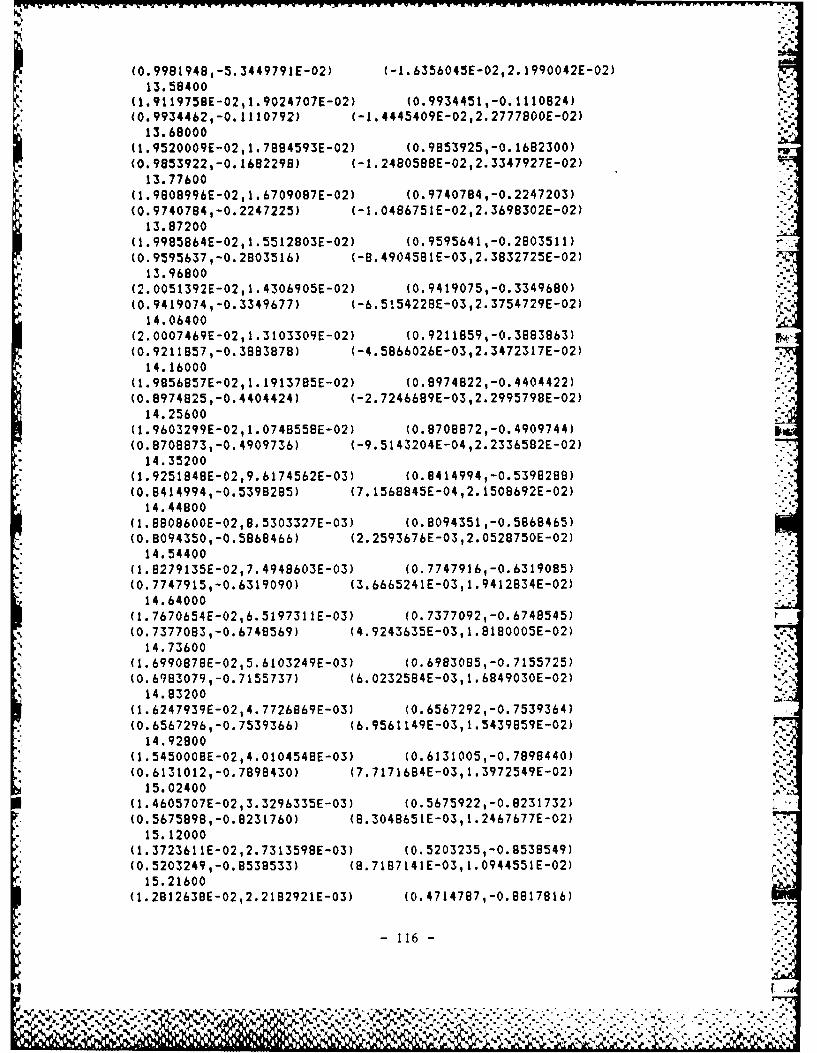
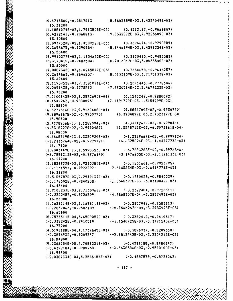
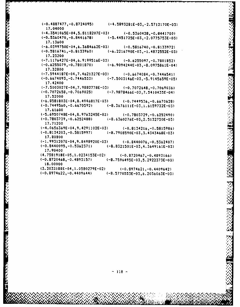
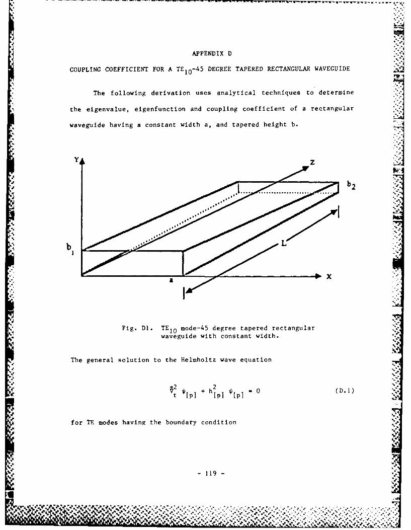
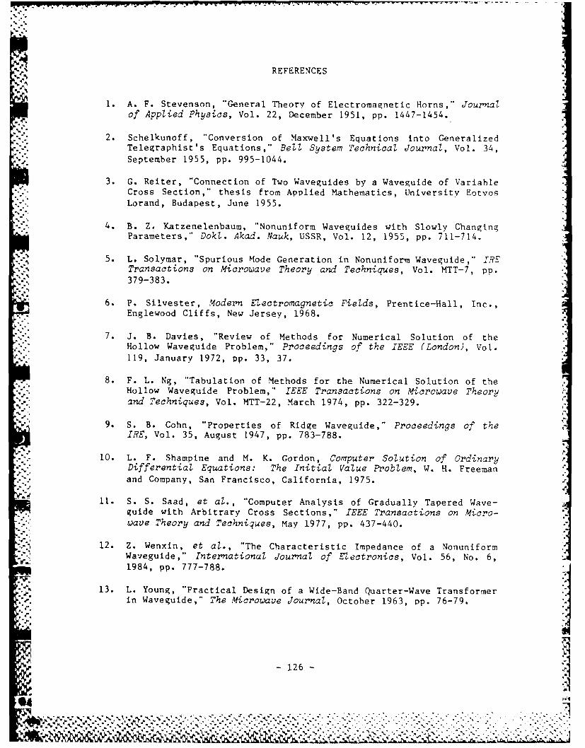


![RADC-TR-90-181 In-House Report - apps.dtic.mil · The two software tools, EMUL and GADAR(1], were delivered by the Hazeltine Corp. under the "Systolic Array Processor Brassboard"](https://static.documents.pub/doc/80x56/5c89126d09d3f2bb368ca5bd/radc-tr-90-181-in-house-report-appsdticmil-the-two-software-tools-emul.jpg)


