Slide 1 of 25

Radial Basis Function Generated Finite Differences (RBF-FD):New Computational Opportunities for Solving PDEs

Bengt Fornberg University of Colorado, Boulder,Department of Applied Mathematics

Natasha Flyer NCAR, IMAGeInstitute for Mathematics Applied to the Geosciences

in collaboration with

Brad Martin, Greg Barnett, and Victor Bayona

New Directions in Numerical Computingin celebration of

Nick Trefethen’s 60th birthday

Slide 2 of 25

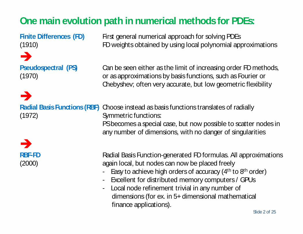
One main evolution path in numerical methods for PDEs:Finite Differences (FD) First general numerical approach for solving PDEs (1910) FD weights obtained by using local polynomial approximations

Pseudospectral (PS) Can be seen either as the limit of increasing order FD methods, (1970) or as approximations by basis functions, such as Fourier or

Chebyshev; often very accurate, but low geometric flexibility

Radial Basis Functions (RBF) Choose instead as basis functions translates of radially (1972) Symmetric functions:

PS becomes a special case, but now possible to scatter nodes in any number of dimensions, with no danger of singularities

RBF-FD Radial Basis Function-generated FD formulas. All approximations (2000) again local, but nodes can now be placed freely

- Easy to achieve high orders of accuracy (4th to 8th order)- Excellent for distributed memory computers / GPUs- Local node refinement trivial in any number of

dimensions (for ex. in 5+ dimensional mathematicalfinance applications).

Slide 3 of 25

Meshes vs. Mesh-free discretizations

Structured meshes:Finite Differences (FD), Discontinuous Galerkin (DG)Finite Volumes (FV)Spectral Elements (SE)

Require domain decomposition / curvilinear mappings

Unstructured meshes:Finite Elements (FE)

Improved geometric flexibility; requires triangles, tetrahedrons, etc.

Mesh-free:Radial Basis Function generated FD (RBF-FD )

Use RBF methods to generate weights inscattered node FD formulasTotal geometric flexibility; needs just scattered nodes, but noconnectivites, e.g. no triangles or mappings

Slide 4 of 25

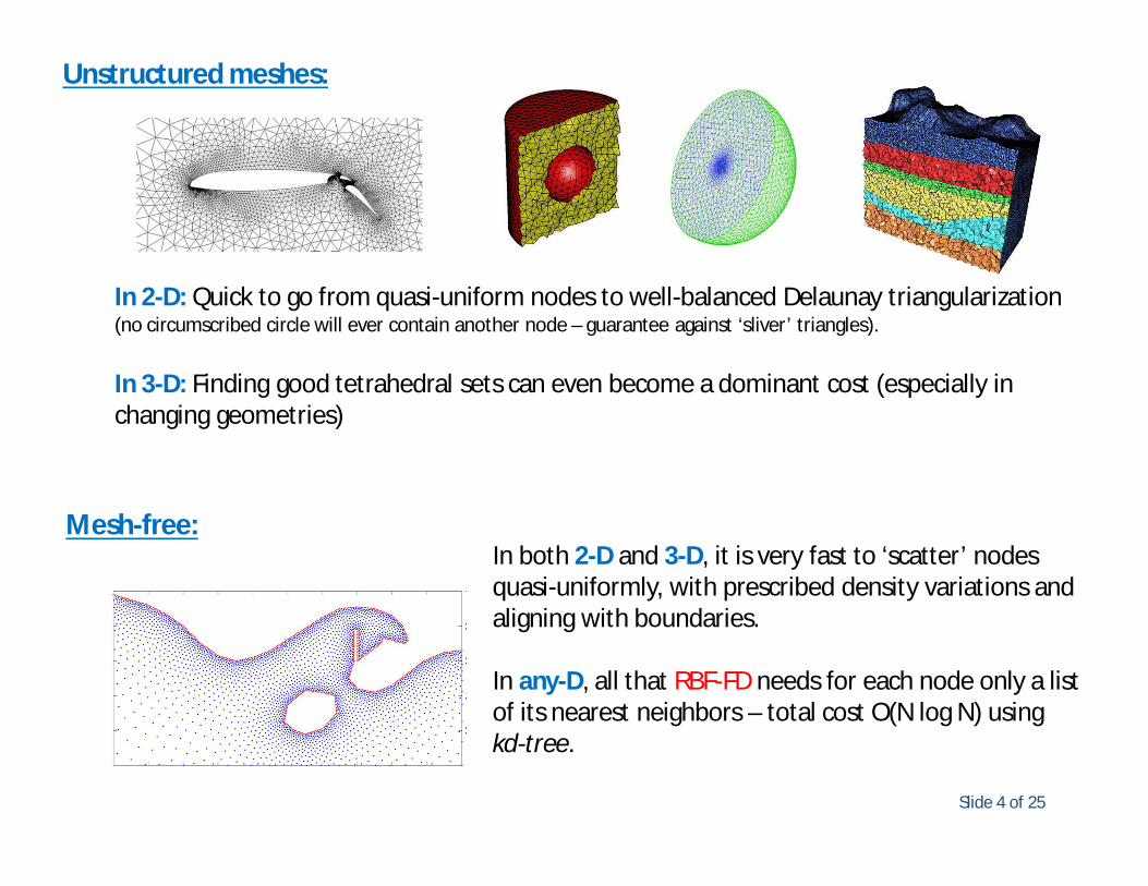
Mesh-free:In both 2-D and 3-D, it is very fast to ‘scatter’ nodes quasi-uniformly, with prescribed density variations and aligning with boundaries.

In any-D, all that RBF-FD needs for each node only a list of its nearest neighbors – total cost O(N log N) using kd-tree.

Unstructured meshes:

In 2-D: Quick to go from quasi-uniform nodes to well-balanced Delaunay triangularization (no circumscribed circle will ever contain another node – guarantee against ‘sliver’ triangles).

In 3-D: Finding good tetrahedral sets can even become a dominant cost (especially in changing geometries)

Slide 5 of 25

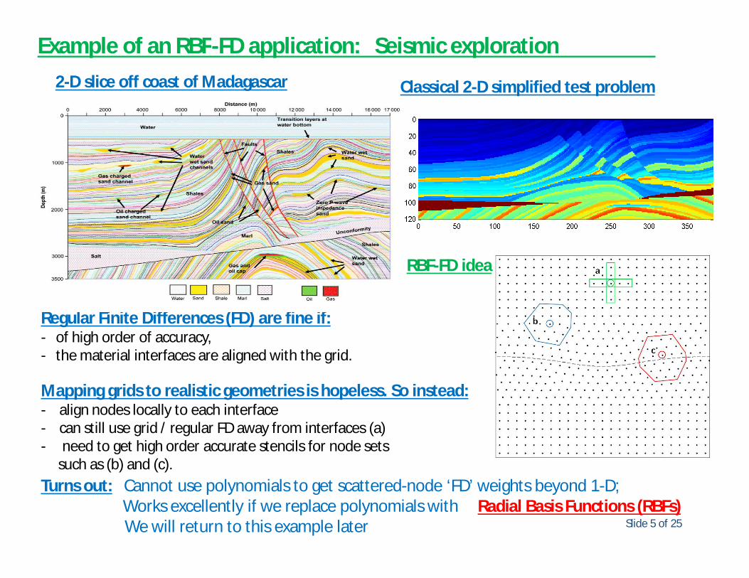
Regular Finite Differences (FD) are fine if:- of high order of accuracy, - the material interfaces are aligned with the grid.

Mapping grids to realistic geometries is hopeless. So instead:- align nodes locally to each interface- can still use grid / regular FD away from interfaces (a)- need to get high order accurate stencils for node sets

such as (b) and (c).

Example of an RBF-FD application: Seismic exploration2-D slice off coast of Madagascar Classical 2-D simplified test problem

RBF-FD idea

Turns out: Cannot use polynomials to get scattered-node ‘FD’ weights beyond 1-D; Works excellently if we replace polynomials with Radial Basis Functions (RBFs)We will return to this example later

Slide 6 of 25

RBF idea, In pictures (for 2-D scattered data):

Scattered data within a 2-D region

Radial basis functions –here ‘rotated’ Gaussians

Linear combination of the basis functions that fits all the data

Many types of RBFs are available; Three examples:

Infinitely smooth RBFs (such as these ones) give spectral accuracy for interpolation and derivative approximations.

Slide 7 of 25

RBF idea, In formulas:

Given scattered data (xk, fk), k = 1,2, … , n ind-D, the RBF interpolant is

1( ) (|| ||)

n

k kk

s x x x

The coefficients lk can be found by collocation:s(xk) = fk, k = 1,2, … , n :

1 1 1 2 1 1 1

2 1 2 2 2 2 2

1 2

(|| ||) (|| ||) (|| ||)(|| ||) (|| ||) (|| ||)

(|| ||) (|| ||) (|| ||)

n

n

n n n n n n

x x x x x x fx x x x x x f

x x x x x x f

Slide 8 of 25

What is so special about expanding in RBFs?

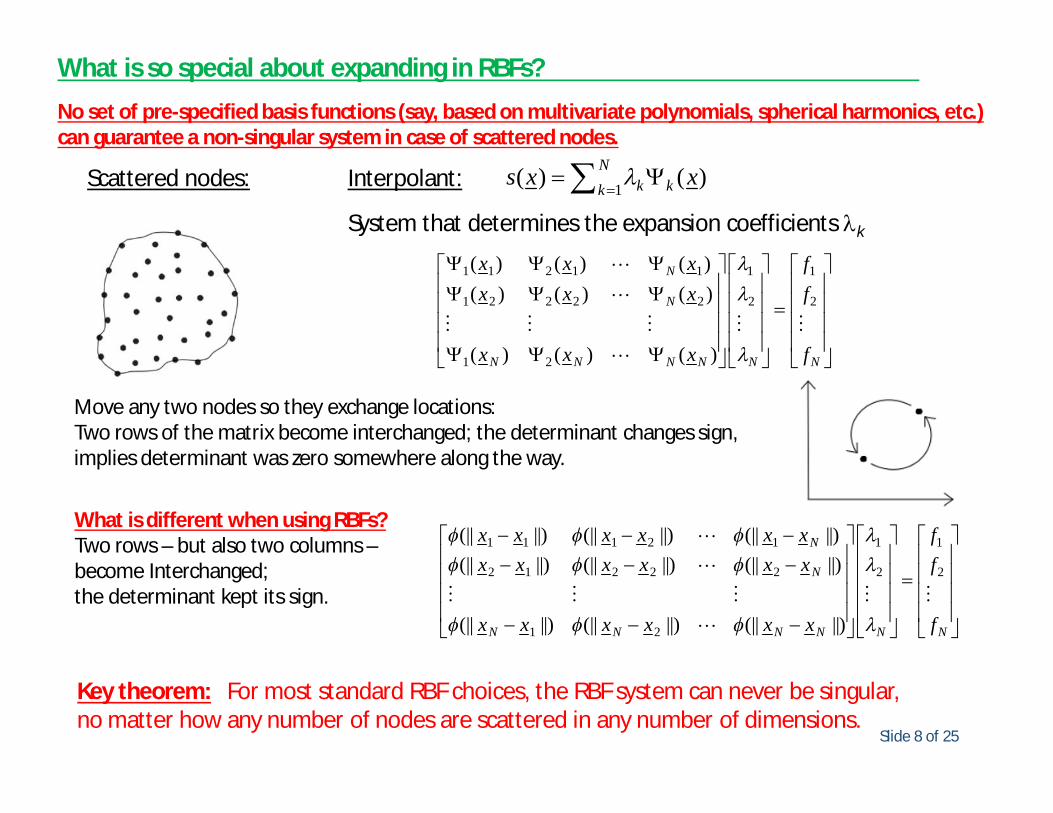
No set of pre-specified basis functions (say, based on multivariate polynomials, spherical harmonics, etc.) can guarantee a non-singular system in case of scattered nodes.

Scattered nodes: Interpolant:

System that determines the expansion coefficients lk

1( ) ( )N

k kks x x

1 1 2 1 1 1 1

1 2 2 2 2 2 2

1 2

( ) ( ) ( )( ) ( ) ( )

( ) ( ) ( )

N

N

N N N N N N

x x x fx x x f

x x x f

1 1 1 2 1 1 1

2 1 2 2 2 2 2

1 2

(|| ||) (|| ||) (|| ||)(|| ||) (|| ||) (|| ||)

(|| ||) (|| ||) (|| ||)

N

N

N N N N N N

x x x x x x fx x x x x x f

x x x x x x f

Move any two nodes so they exchange locations:Two rows of the matrix become interchanged; the determinant changes sign,implies determinant was zero somewhere along the way.

What is different when using RBFs?Two rows – but also two columns –become Interchanged; the determinant kept its sign.

Key theorem: For most standard RBF choices, the RBF system can never be singular, no matter how any number of nodes are scattered in any number of dimensions.

Slide 9 of 25

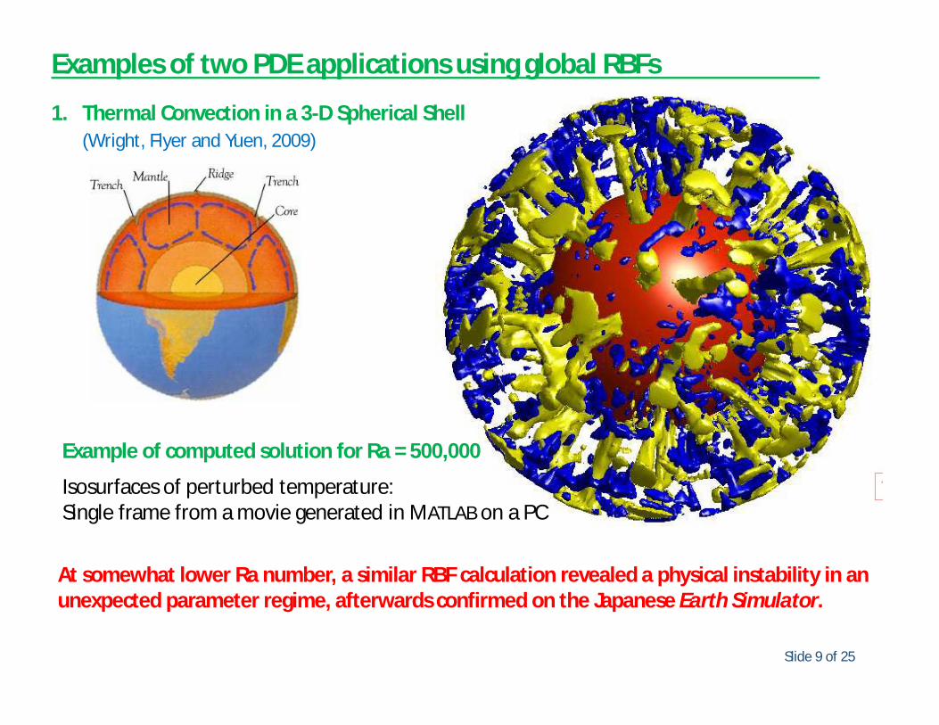
Examples of two PDE applications using global RBFs

1. Thermal Convection in a 3-D Spherical Shell(Wright, Flyer and Yuen, 2009)

Example of computed solution for Ra = 500,000

Isosurfaces of perturbed temperature:Single frame from a movie generated in MATLAB on a PC

At somewhat lower Ra number, a similar RBF calculation revealed a physical instability in an unexpected parameter regime, afterwards confirmed on the Japanese Earth Simulator.

Slide 10 of 25

Another global RBF example: Reaction-diffusion equations over curved biological surfaces(Piret, 2012)

The Brusselator equation, modeling pattern formation, is solved here by global RBFs over the surface of a frog

- The 560 scattered nodes serve both as collocation points and to define the body shape- Spectral accuracy: Only 2 points are needed per wave length to be resolved

Top row:Snapshots from a computed time evolution for two different parameter values

Bottom row:Left: Tabasara rain frogRight: Poison dart frog

Slide 11 of 25

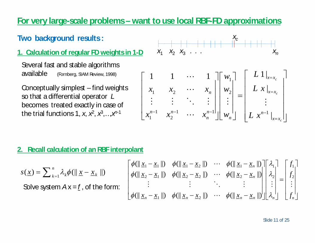
For very large-scale problems – want to use local RBF-FD approximations

1( ) (|| ||)n

kkks x x x

1 1 1 2 1 1 1

2 1 2 2 2 2 2

1 2

(|| ||) (|| ||) (|| ||)(|| ||) (|| ||) (|| ||)

(|| ||) (|| ||) (|| ||)

n

n

n n n n n n

fx x x x x xfx x x x x x

fx x x x x x

Solve system A x = f , of the form:

1. Calculation of regular FD weights in 1-D

2. Recall calculation of an RBF interpolant

xc

x1 x2 x3 . . . xn

Several fast and stable algorithmsavailable (Fornberg, SIAM Review, 1998)

Conceptually simplest – find weightsso that a differential operator Lbecomes treated exactly in case ofthe trial functions 1, x, x2, x3,…,xn-1

1

1 2 2

1 1 1 11 2

1 |1 1 1|

|

c

c

c

x x

x xn

n n n nn n x x

LwL xx x x w

x x x w L x

Two background results :

Slide 12 of 25

Calculation of weights in RBF-FD stencil for a differential operator L

11 1 1

1

1 2

1 3

(|| ||) |1

(|| ||) |11 |1 1

0 |

|

c

c

c

c

c

x x

n x xn n n

x xn

n n x x

n n x x

L x xx y wA

L x xx y wLw

x x w Lxy y w Ly

System to solve for weights in case of 2-D, when also using up to linear polynomials with corresponding constraints

Same A-matrix as above; the entries wn+1, … should be ignored.

Common RBF types: Infinitely smooth, e.g. GA: , MQ:

or finitely smooth, e.g. PHS:

2( )( ) rr e 2( ) 1 ( )r r 2 2 1( ) log , ( ) .m mr r r r r

Choose weights so the result becomesExact for all RBFs interpolants of the form

with constraints

1( ) (|| ||) ( )n

kk mks x x x p x

( ) 0k m kp x

Some observations when using PHS with supporting polynomials:

- Non-singularity of linear system again assured,- When refining, the polynomial part gradually ‘takes over’ from RBF part,- With PHS, can use one-sided approximations at boundaries – a spline-like absence of Runge

phenomenon.

Slide 13 of 25

Convective flow around a sphere with the RBF-FD method(Fornberg and Lehto, 2011)

Test problem: Solid body rotation around a sphere Initial condition: Cosine bell: N = 25,600, n = 74, RK4 in time

RBF-FD stencil illustration: N = 800 ME nodes, n = 30. No surface bound coordinate system usedno counterpart to pole singularities

Numerical solution:- No visible loss in peak height, or of trailing wave trains- For given accuracy, the most cost effective method available

Slide 14 of 25

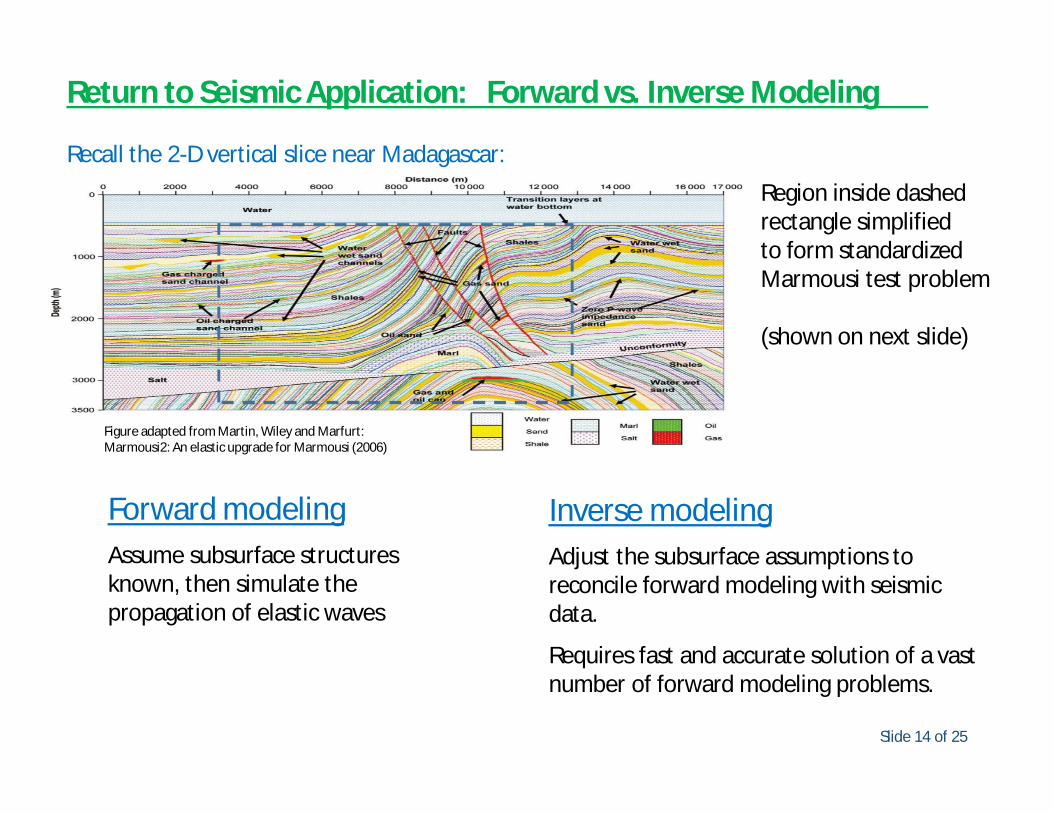
Return to Seismic Application: Forward vs. Inverse Modeling

Recall the 2-D vertical slice near Madagascar:

Region inside dashedrectangle simplifiedto form standardizedMarmousi test problem

(shown on next slide)

Figure adapted from Martin, Wiley and Marfurt: Marmousi2: An elastic upgrade for Marmousi (2006)

Forward modelingAssume subsurface structures known, then simulate the propagation of elastic waves

Inverse modelingAdjust the subsurface assumptions to reconcile forward modeling with seismic data.

Requires fast and accurate solution of a vast number of forward modeling problems.

Slide 15 of 25

Governing equations for elastic wave propagation in 2-D2blem

Elastic wave equation in 2-D

( 2 )( )

( 2 )

t x y

t x y

t x y

t x y

t y x

u f gv g h

f u vg u vh v u

Dependent variables:u, v horizontal and vertical velocitiesf, g, h components of the symmetric

stress tensor

Material parameters:r densityl, m Lamé parameters (compression and shear)

Wave types:Pressure , ShearAlso: Rayleigh, Love, and Stonley waves

( 2 ) /pc /sc

Acoustic (pressure wave) velocities ↑

Slide 16 of 25

Region Type Dominant Errors Computational Remedies

Smoothly variable medium

Dispersive errors High order approximations1980’s From 2nd order to 4th order FD (or FEM)2010’s 20th order (or higher still) FD

Interfaces Reflection and transmission of pressure and shear waves

Analysis based interface enhancements on grids:Very limited successes reported in the literaturein cases of complex geometries

Industry standard: Refine and ‘hope for the best’ (typically 1st order)

Present novelties:

- Distribute RBF-FD nodes to align with all interfaces(suffices for 2nd order)

- Modify basis functions to analytically correct forinterface conditions (RBF-FD/AC) (high order possible also for curved interfaces)

(Martin, Fornberg, St-Cyr, 2015)

Slide 17 of 25

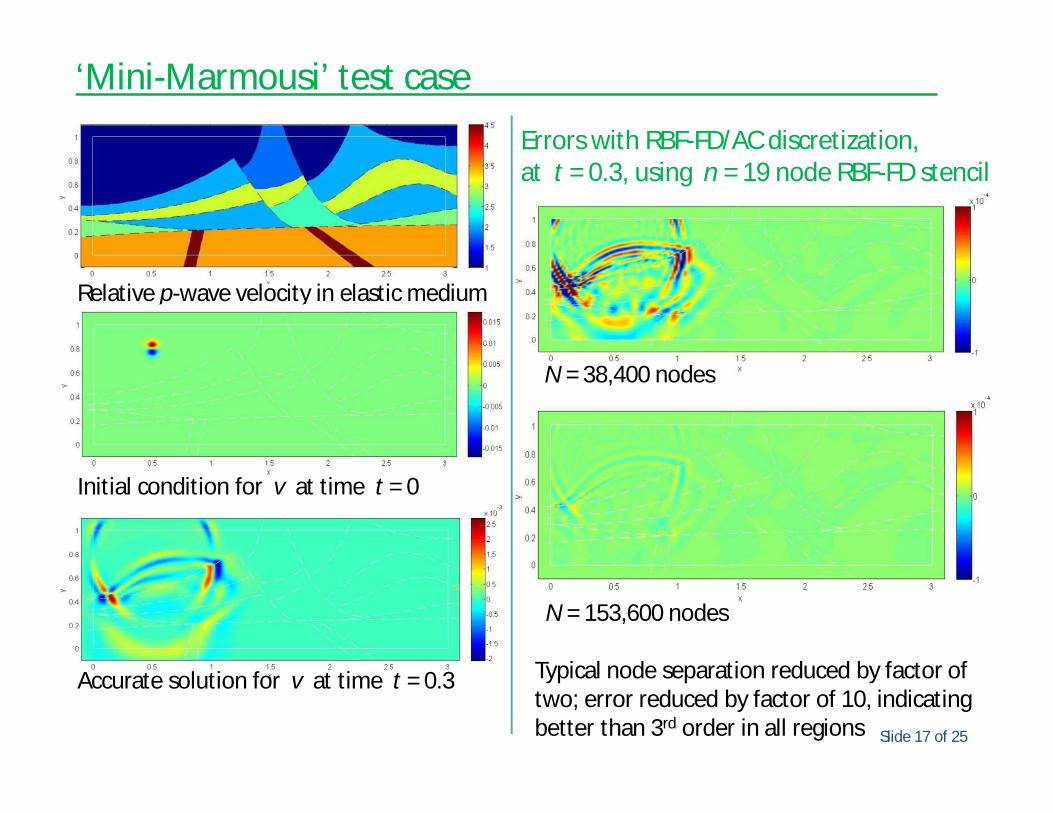
‘Mini-Marmousi’ test case

Relative p-wave velocity in elastic medium

Initial condition for v at time t = 0

Accurate solution for v at time t = 0.3

N = 38,400 nodes

Errors with RBF-FD/AC discretization, at t = 0.3, using n = 19 node RBF-FD stencil

N = 153,600 nodes

Typical node separation reduced by factor of two; error reduced by factor of 10, indicatingbetter than 3rd order in all regions

Slide 18 of 25

3-D acoustic wave equation, solved by the RBF-FD/AC procedure

Ricker wavelet initial condition at location (0.5, 0.5, 0.75) Material interface is here an inclined flat plane, RBF-FD/AC with N = 106, n = 61.

Views from two different angles of the RBF-FD/AC solution at a later time:

Slide 19 of 25

Timing comparison against FD20 (FD of 20th order of accuracy) 3-D acoustic test problem

CPU vs. GPU:

FD20: Very wide stencils; large domain overlaps ; lots of communicationsRBF-FD: The opposite in all regards; utilizes GPUs more effectively (in spite of scattered nodes)

Slide 20 of 25

Modeling 2D nonhydrostatic compressible Navier-Stokes(Flyer, Barnett, Wicker, 2015)

Accurate time evolution

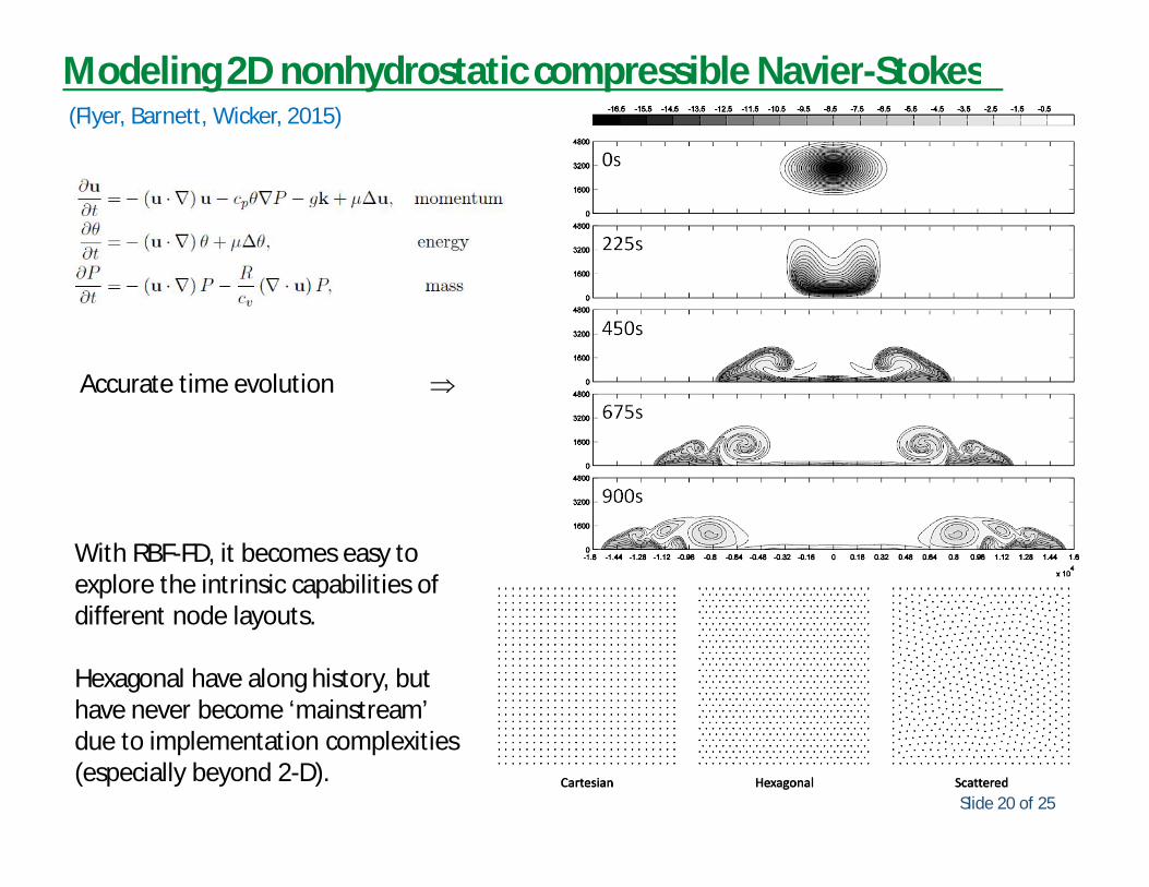
With RBF-FD, it becomes easy to explore the intrinsic capabilities of different node layouts.

Hexagonal have along history, but have never become ‘mainstream’ due to implementation complexities (especially beyond 2-D).

Slide 21 of 25

Comparisons on different node layouts

RBFs : 풓ퟕ with 4th degree polynomial support, n = 37, ∆ퟑ-type hyperviscosity

For comparable node numbers:- Cartesian node layout gives rise to the most amount of unphysical artifacts- Hexagonal nodes excellent (in the past, too complex to be used routinely –

now similar concept easily used also in 3-D)- No detectable performance penalty when going to quasi-uniformly scattered

(but have then gained great geometric flexibility).

Slide 22 of 25

Comparisons to other numerical methods

At high resolutions, 100m and under, most methods perform well.The key issue for large applications becomes their performance at coarse resolutions. Below: Comparisons from the literature, at 400m resolution?

At this coarse resolution, only the RBF-FD calculations shows the beginning of second rotor (does it on Cartesian, hexagonal, and scattered node sets).

Slide 23 of 25

Same test problem, but with physical viscosity removed altogether

Modeling 2D nonhydrostatic compressible Euler equations – 25m resolution (RBF-FD, hex nodes)

Details when using different resolutions

Slide 24 of 25

ConclusionsEstablished:

- There is a natural method evolution: FD PS RBF RBF-FD

- RBF and RBF-FD methods combine high accuracy with great flexibility for handling intricate geometries and local refinement

- RBF and RBF-FD methods compete very favorably against previous methods on a large number of established benchmark problems

- RBF-FD particularly effective on GPUs and other massively parallel hardware

Some examples of recent RBF-FD applications not touched on in this talk:

- Quadrature over closed curved surfaces:O(h7) accuracy in O(N log N) operations (Reeger and Fornberg, 2015).

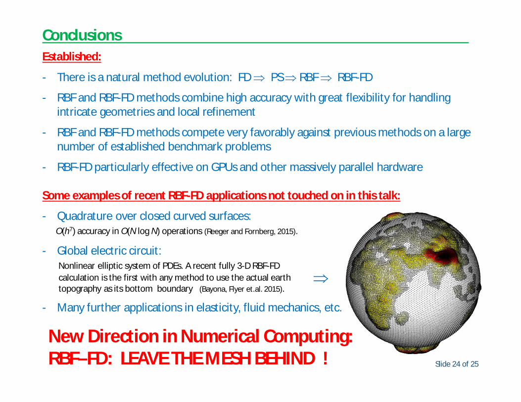
- Global electric circuit: Nonlinear elliptic system of PDEs. A recent fully 3-D RBF-FD calculation is the first with any method to use the actual earth topography as its bottom boundary (Bayona, Flyer et.al. 2015).

- Many further applications in elasticity, fluid mechanics, etc.

New Direction in Numerical Computing:RBF–FD: LEAVE THE MESH BEHIND !

Slide 25 of 25

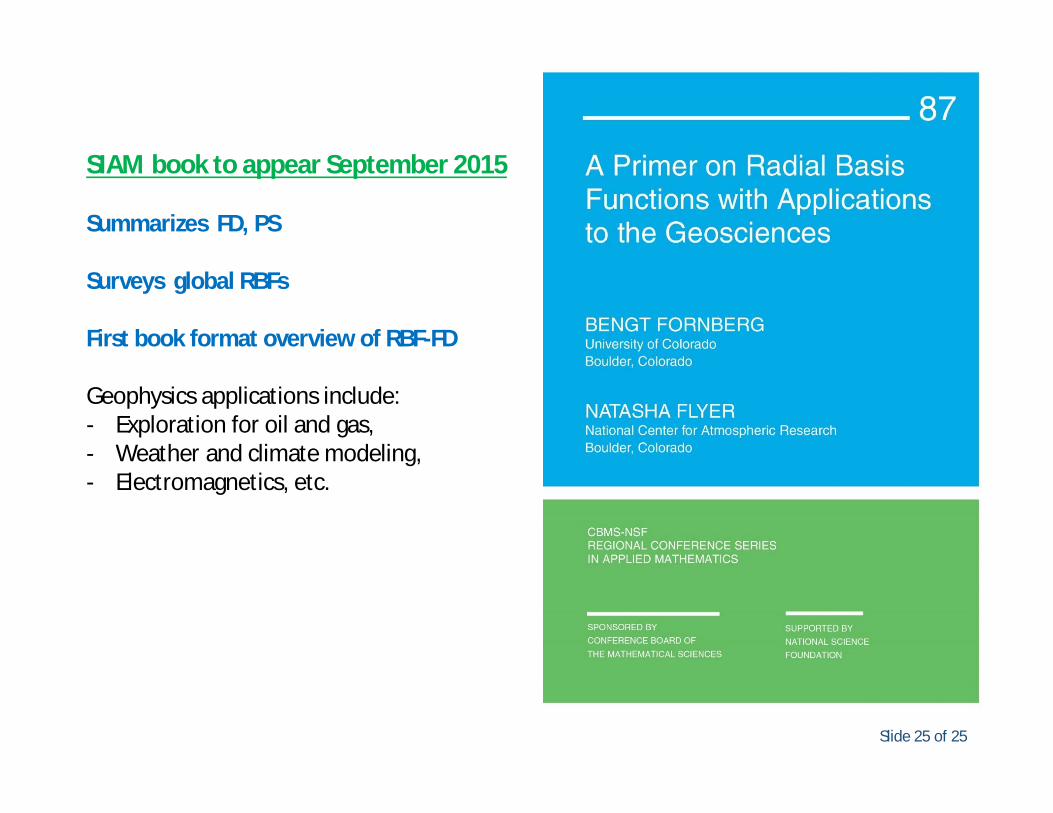
SIAM book to appear September 2015

Summarizes FD, PS

Surveys global RBFs

First book format overview of RBF-FD

Geophysics applications include:- Exploration for oil and gas,- Weather and climate modeling,- Electromagnetics, etc.