96
Radial Velocity Detection of Planets: I. Techniques and Tools 1. Keplerian Orbits 2. Spectrographs/Doppler shifts 3. Precise Radial Velocity measurements 4. Searching for periodic signals
| Date post: | 05-Jan-2016 |
| Category: |
Documents |
| Upload: | martha-whitehead |
| View: | 235 times |
| Download: | 0 times |
Radial Velocity Detection of Planets:I. Techniques and Tools
1. Keplerian Orbits
2. Spectrographs/Doppler shifts
3. Precise Radial Velocity measurements
4. Searching for periodic signals
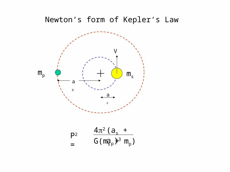
ap
as
V
P2 = 42 (as + ap)3
G(ms + mp)
msmp
Newton‘s form of Kepler‘s Law
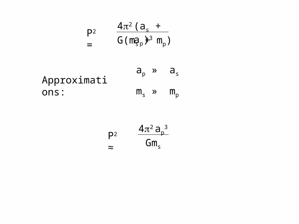
P2 = 42 (as + ap)3
G(ms + mp)
Approximations:ap » as
ms » mp
P2 ≈ 42 ap
3
Gms
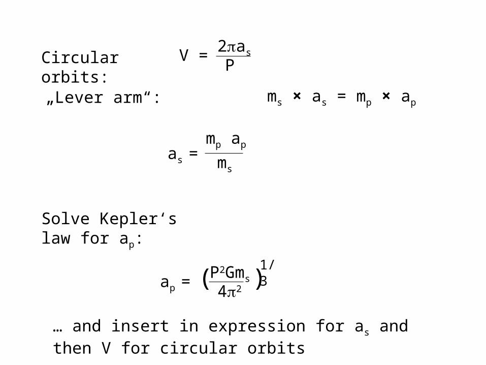
Circular orbits: V = 2as
P
„Lever arm“: ms × as = mp × ap
as = mp ap
ms
Solve Kepler‘s law for ap:
ap = P2Gms
42( )
1/3
… and insert in expression for as and then V for circular orbits
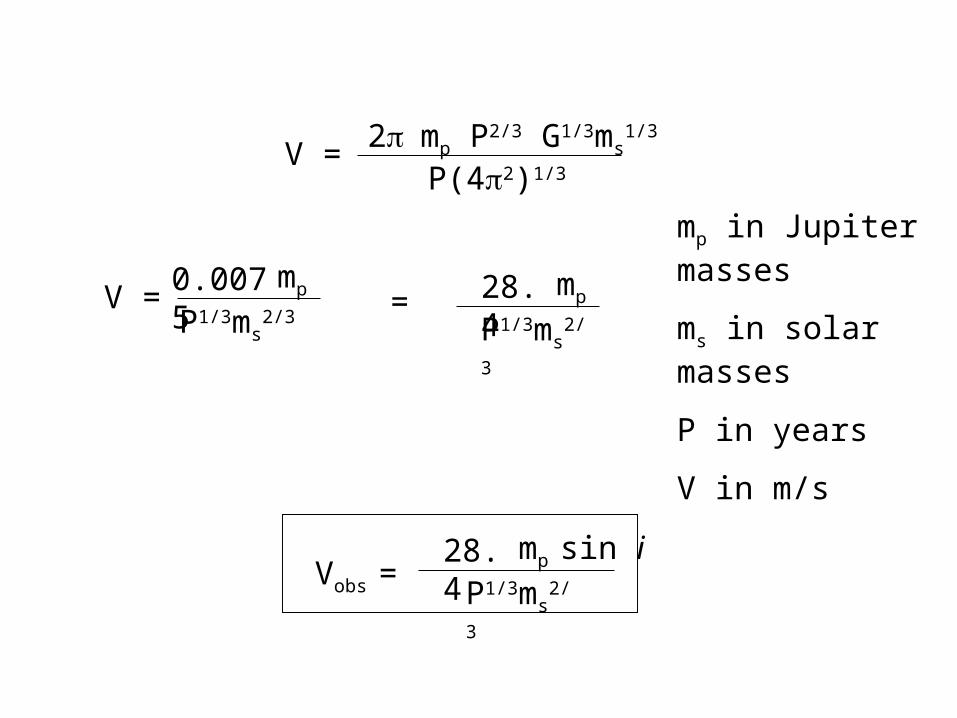
V = 2P(42)1/3
mp P2/3 G1/3ms1/3
V = 0.0075P1/3ms
2/3
mp = 28.4P1/3ms
2/3
mp
mp in Jupiter masses
ms in solar masses
P in years
V in m/s
28.4P1/3ms
2/3
mp sin iVobs =
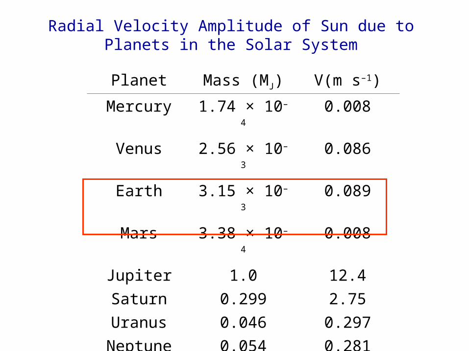
Planet Mass (MJ) V(m s–1)
Mercury 1.74 × 10⁻⁴ 0.008
Venus 2.56 × 10⁻³ 0.086
Earth 3.15 × 10⁻³ 0.089
Mars 3.38 × 10⁻⁴ 0.008
Jupiter 1.0 12.4
Saturn 0.299 2.75
Uranus 0.046 0.297
Neptune 0.054 0.281
Radial Velocity Amplitude of Sun due to Planets in the Solar System
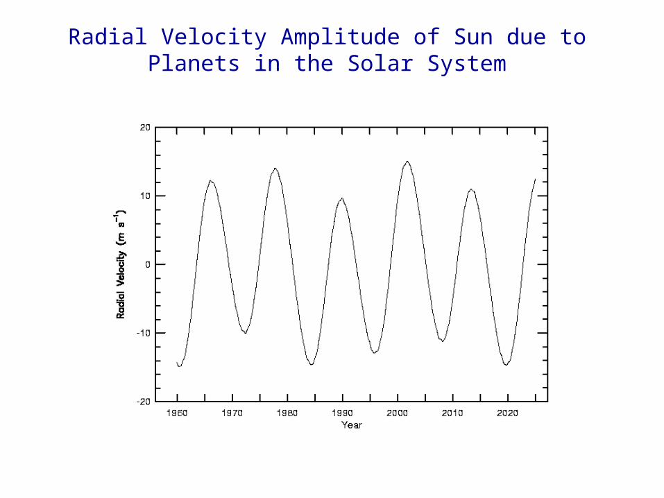
Radial Velocity Amplitude of Sun due to Planets in the Solar System
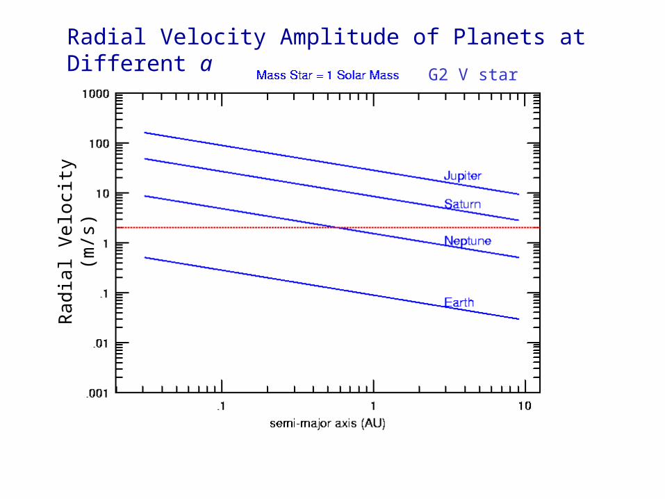
Radial Velocity Amplitude of Planets at Different aR
adia
l Vel
ocity
(m
/s)
G2 V star

Rad
ial V
eloc
ity (
m/s
)A0 V star
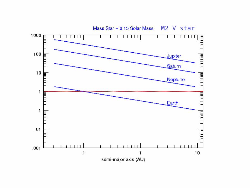
M2 V star
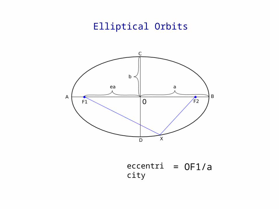
eccentricity
Elliptical Orbits
= OF1/a
O
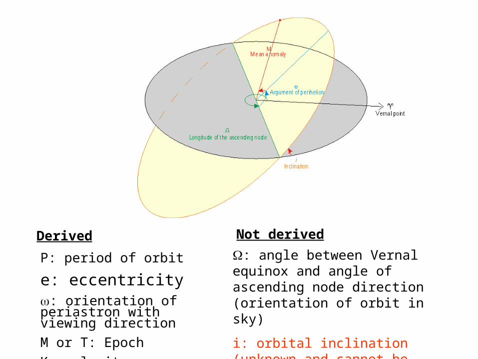
P: period of orbit
e: eccentricity: orientation of periastron with viewing direction
M or T: Epoch
K: velocity amplitude
Derived
: angle between Vernal equinox and angle of ascending node direction (orientation of orbit in sky)
i: orbital inclination (unknown and cannot be determined
Not derived
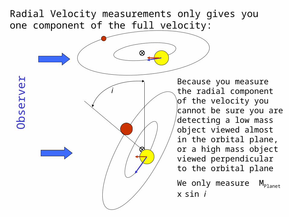
Obs
e rve
r Because you measure the radial component of the velocity you cannot be sure you are detecting a low mass object viewed almost in the orbital plane, or a high mass object viewed perpendicular to the orbital plane
We only measure MPlanet x sin i
i
Radial Velocity measurements only gives you one component of the full velocity:
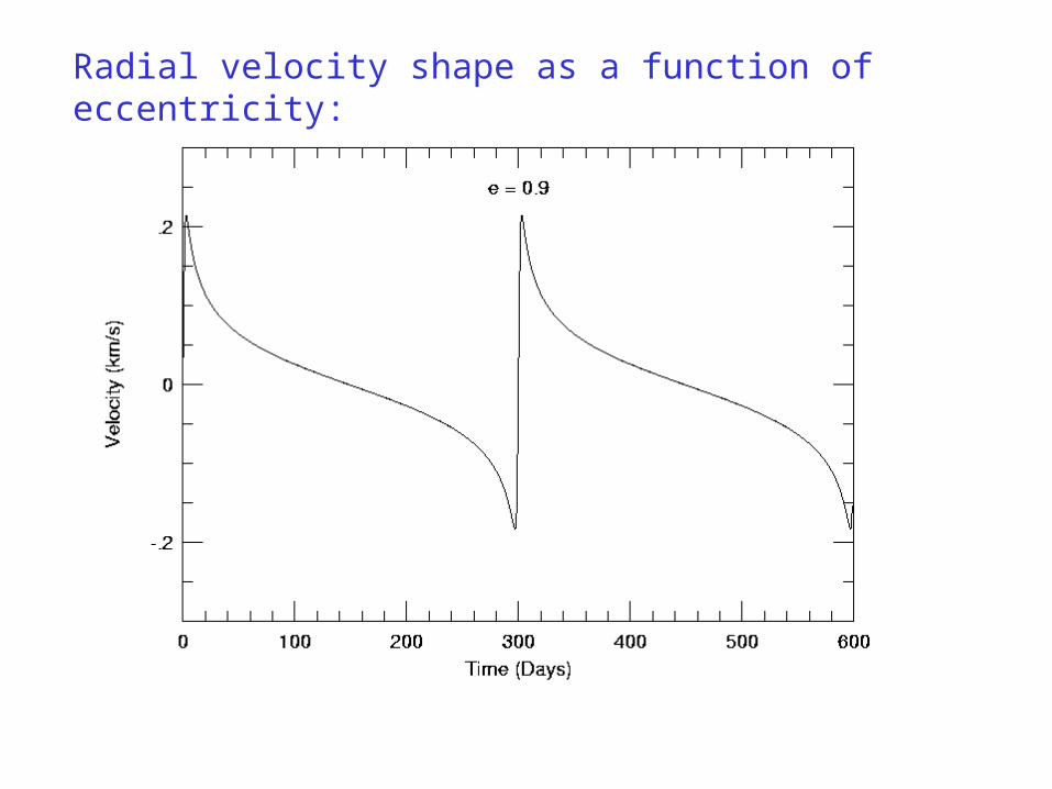
Radial velocity shape as a function of eccentricity:

Radial velocity shape as a function of , e = 0.7 :
radialvelocitysimulator.htm
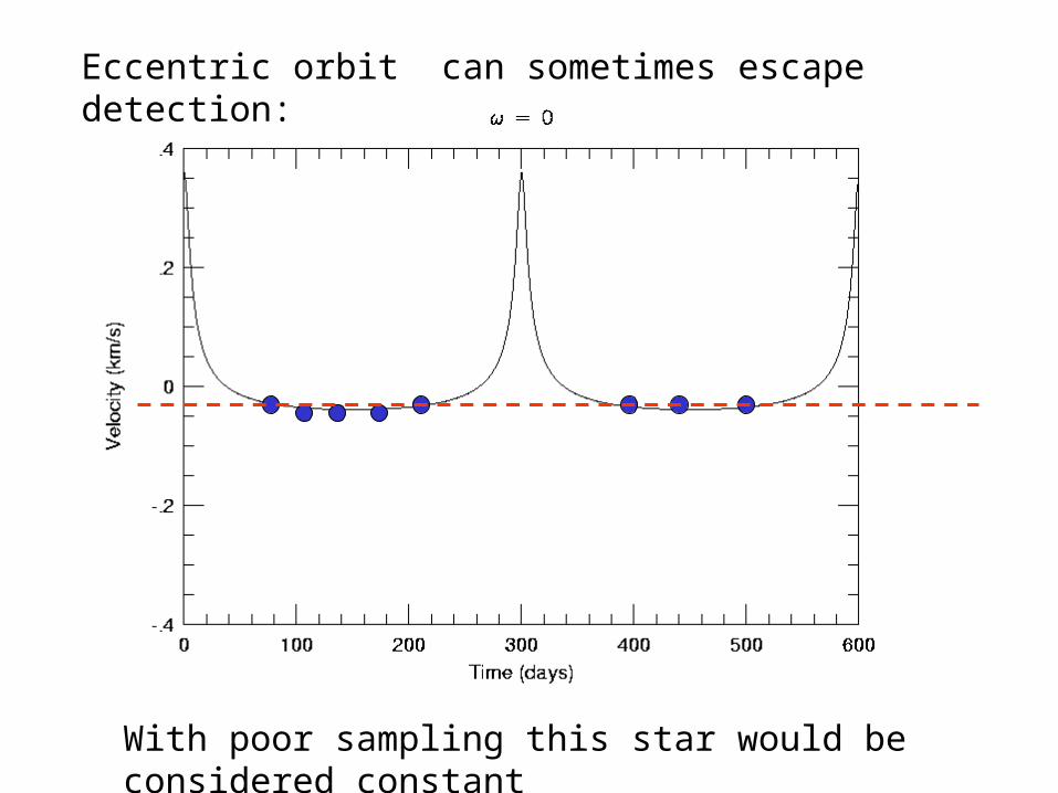
Eccentric orbit can sometimes escape detection:
With poor sampling this star would be considered constant
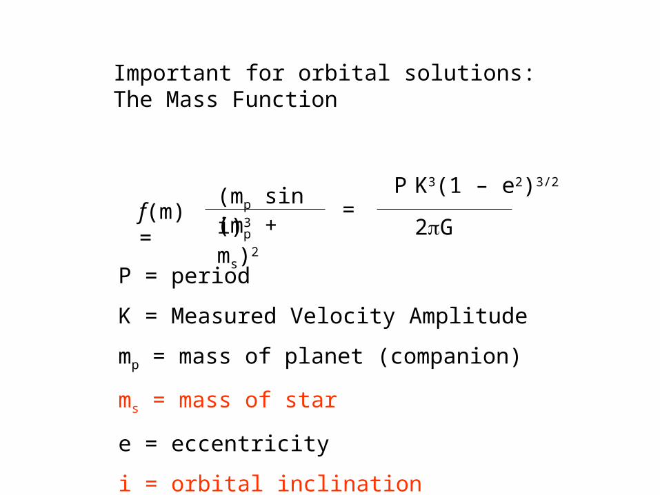
Important for orbital solutions: The Mass Function
f(m) = (mp sin i)3
(mp + ms)2=
P
2G
K3(1 – e2)3/2
P = period
K = Measured Velocity Amplitude
mp = mass of planet (companion)
ms = mass of star
e = eccentricity
i = orbital inclination
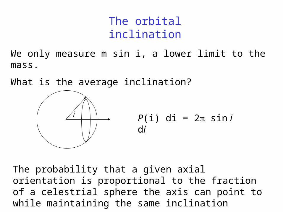
The orbital inclination
We only measure m sin i, a lower limit to the mass.
What is the average inclination?
i
The probability that a given axial orientation is proportional to the fraction of a celestrial sphere the axis can point to while maintaining the same inclination
P(i) di = 2 sin i di
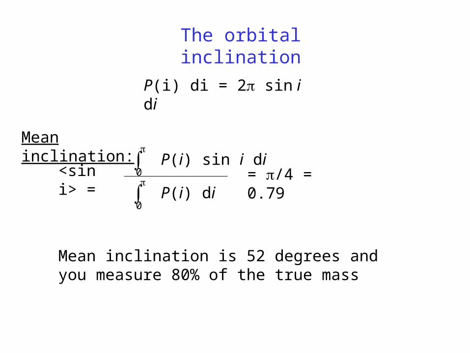
The orbital inclination
P(i) di = 2 sin i di
Mean inclination:
<sin i> =
∫ P(i) sin i di0
∫ P(i) di0
= /4 = 0.79
Mean inclination is 52 degrees and you measure 80% of the true mass
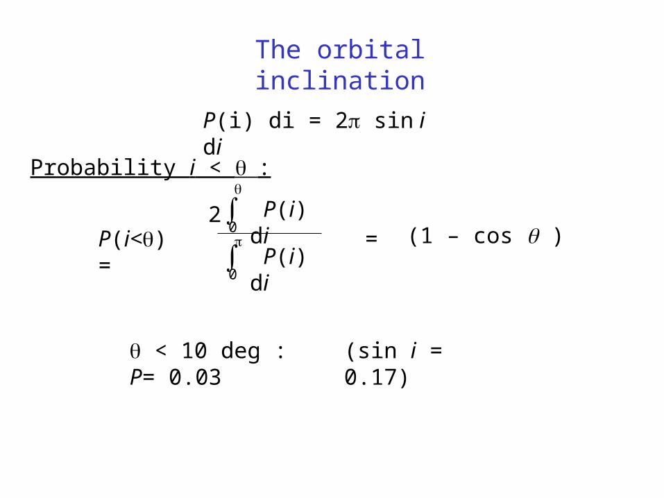
The orbital inclination
P(i) di = 2 sin i di
Probability i < :
P(i<) =
∫ P(i) di0
∫ P(i) di0
2(1 – cos ) =
< 10 deg : P= 0.03 (sin i = 0.17)
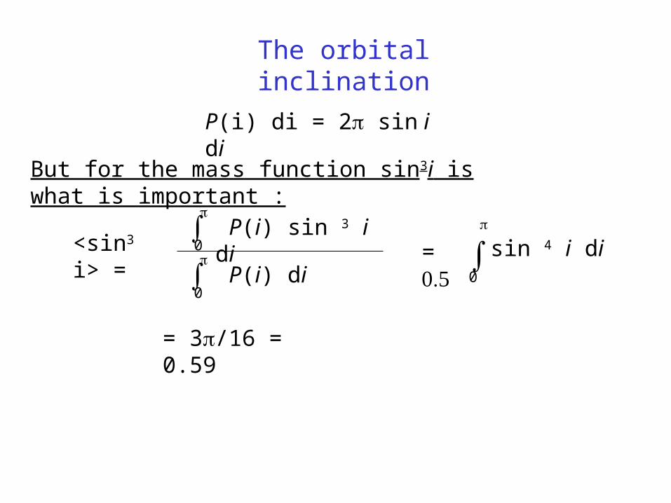
The orbital inclination
P(i) di = 2 sin i di
But for the mass function sin3i is what is important :
<sin3 i> =
∫ P(i) sin 3 i di0
∫ P(i) di0
= ∫ sin 4 i di
0
= 3/16 = 0.59
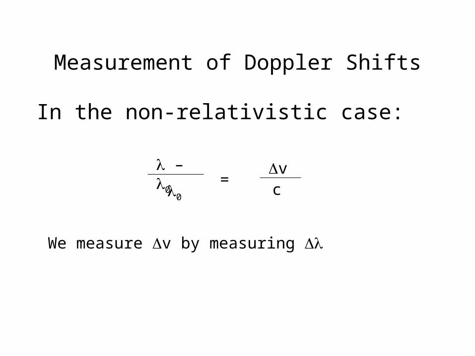
Measurement of Doppler Shifts
In the non-relativistic case:
– 0
0
= vc
We measure v by measuring
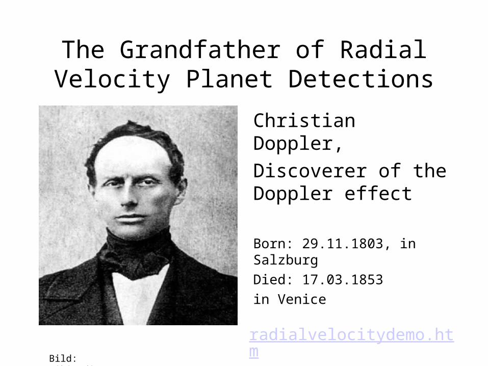
The Grandfather of Radial Velocity Planet Detections
Christian Doppler,
Discoverer of the Doppler effect
Born: 29.11.1803, in Salzburg
Died: 17.03.1853
in Venice
radialvelocitydemo.htmBild: Wikipedia
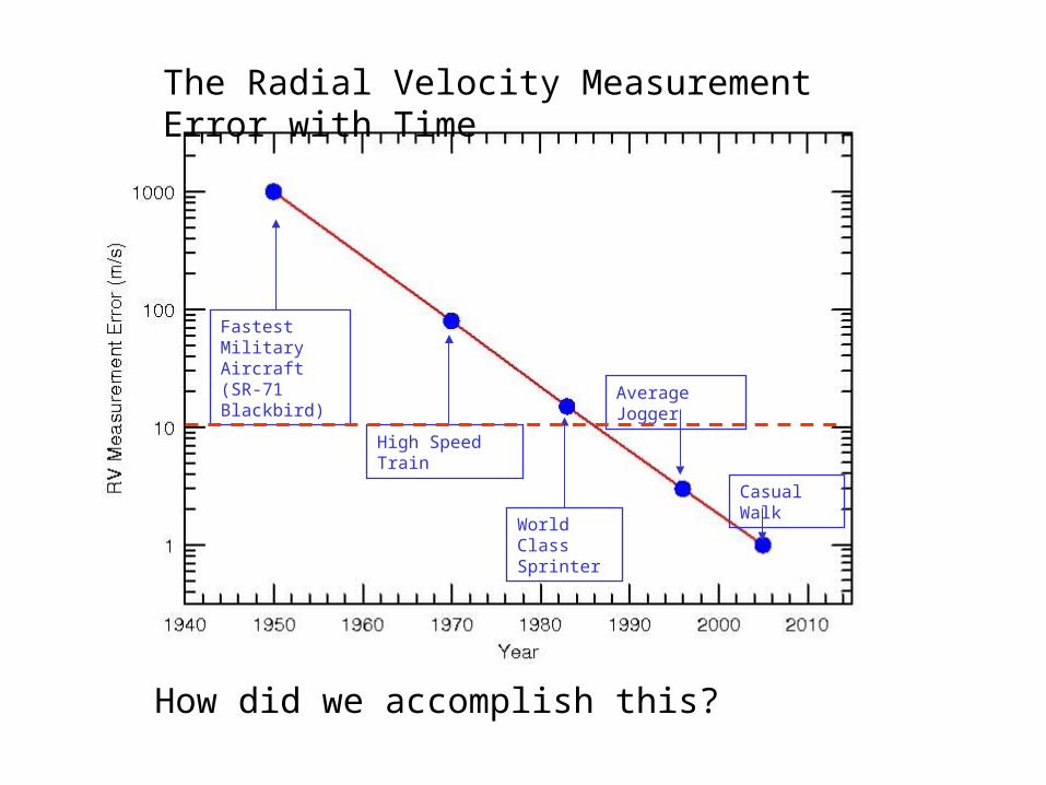
The Radial Velocity Measurement Error with Time
How did we accomplish this?
Fastest Military Aircraft (SR-71 Blackbird)
High Speed Train
World Class Sprinter
Casual Walk
Average Jogger
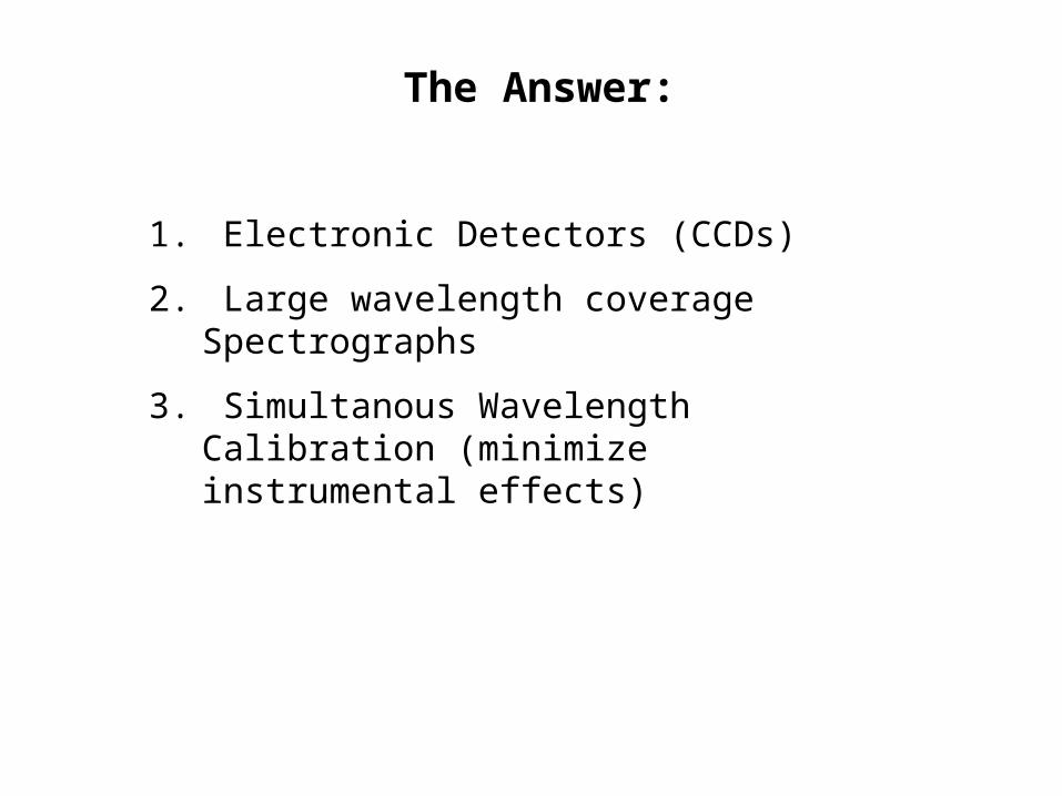
The Answer:
1. Electronic Detectors (CCDs)
2. Large wavelength coverage Spectrographs
3. Simultanous Wavelength Calibration (minimize instrumental effects)
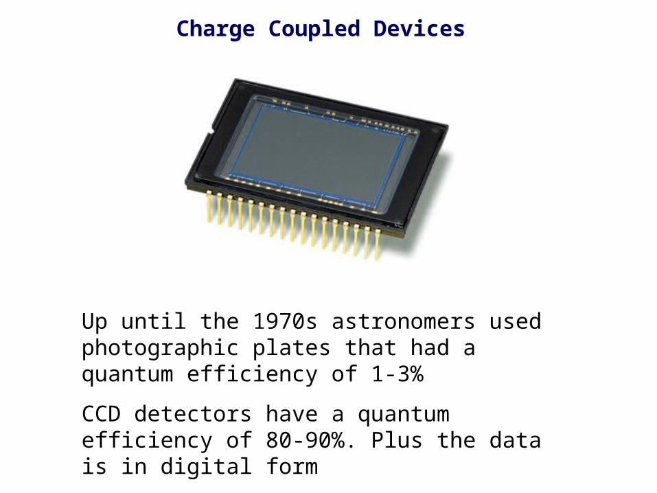
Charge Coupled Devices
Up until the 1970s astronomers used photographic plates that had a quantum efficiency of 1-3%
CCD detectors have a quantum efficiency of 80-90%. Plus the data is in digital form
Instrumentation for Doppler Measurements
High Resolution Spectrographs with Large Wavelength Coverage
collimator
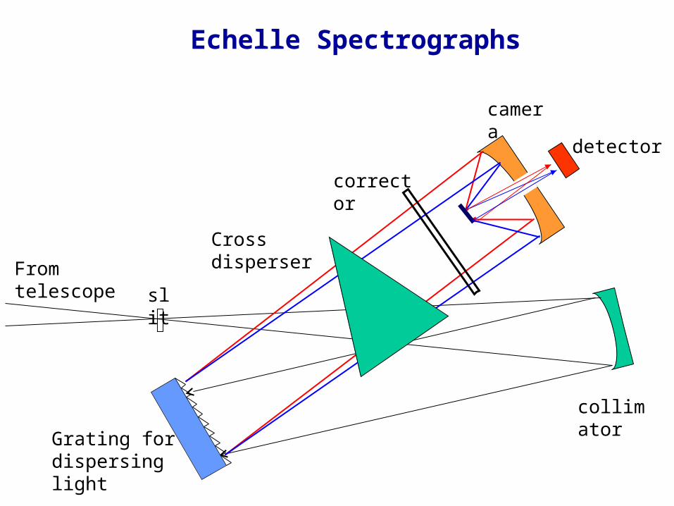
Echelle Spectrographs
slit
camera
detector
corrector
From telescope
Cross disperser
Grating for dispersing light
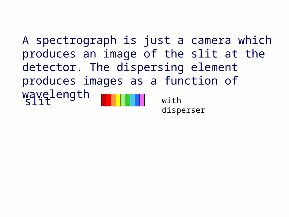
A spectrograph is just a camera which produces an image of the slit at the detector. The dispersing element produces images as a function of wavelength
without disperserwith disperserslit
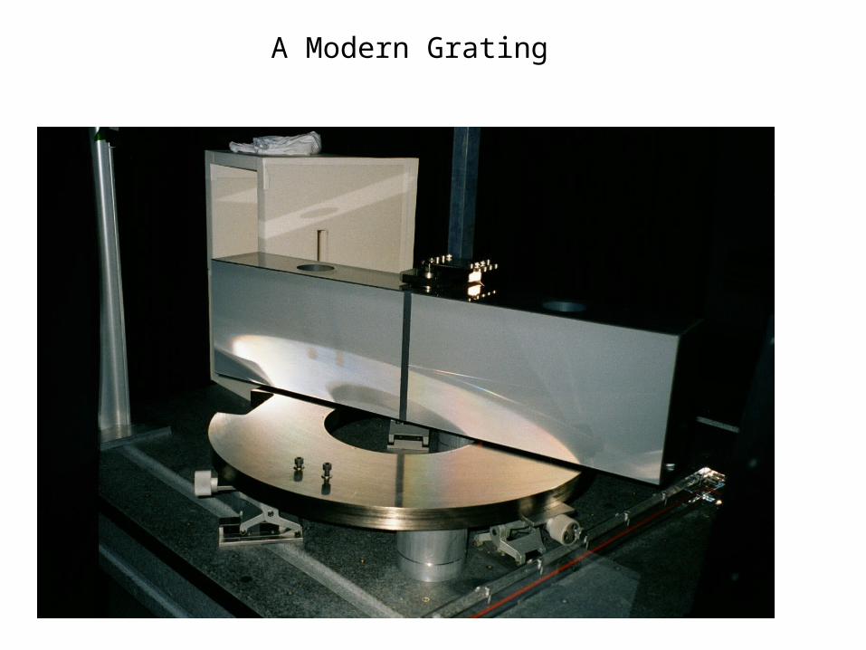
A Modern Grating
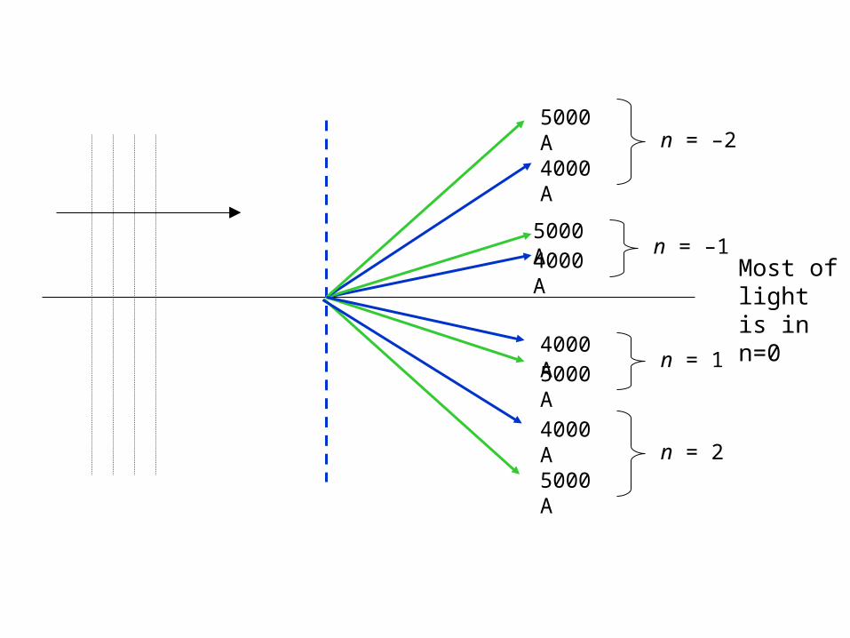
5000 A
4000 An = –1
5000 A
4000 An = –2
4000 A
5000 An = 2
4000 A
5000 An = 1
Most of light is in n=0
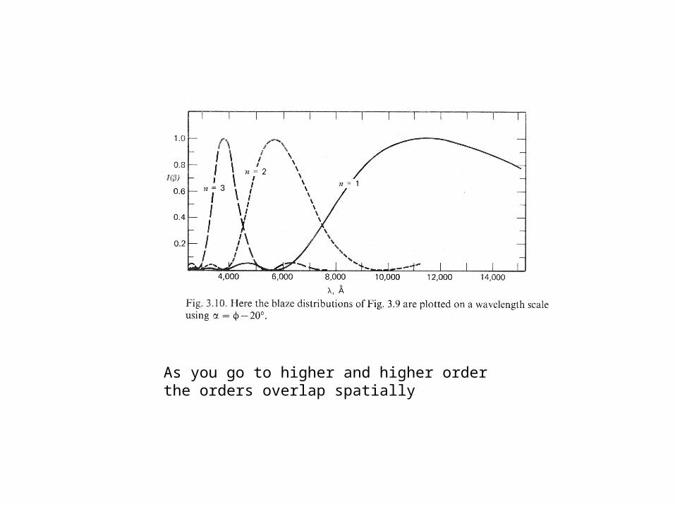
As you go to higher and higher order the orders overlap spatially
3000
m=3
5000
m=2
4000 9000
m=1
6000 14000Schematic: orders separated in the vertical direction for clarity
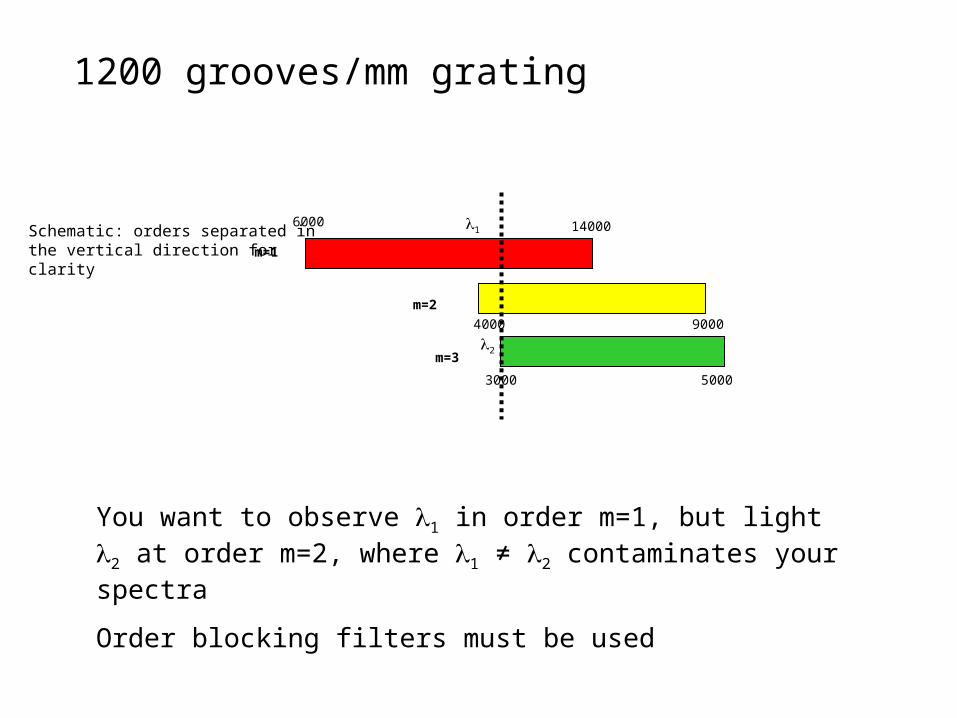
1200 grooves/mm grating
2
1
You want to observe 1 in order m=1, but light 2 at order m=2, where 1 ≠ 2 contaminates your spectra
Order blocking filters must be used
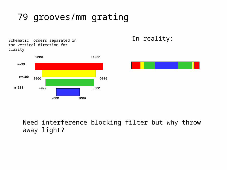
4000
m=99
m=100
m=101 5000
5000 9000
9000 14000
Schematic: orders separated in the vertical direction for clarity
79 grooves/mm grating
30002000
Need interference blocking filter but why throw away light?
In reality:

y ∞ 2
y
m-2
m-1
m
m+2
m+3
Free Spectral Range m
Grating cross-dispersed echelle spectrographs
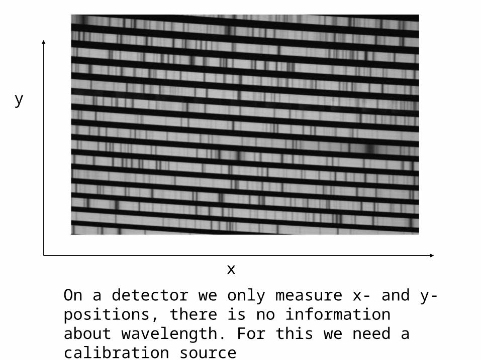
On a detector we only measure x- and y- positions, there is no information about wavelength. For this we need a calibration source
y
x
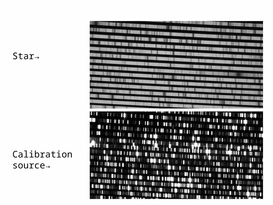
Star→
Calibration source→
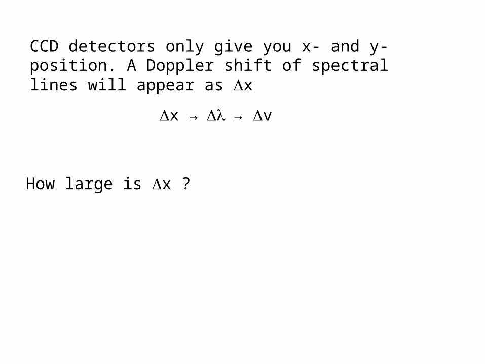
CCD detectors only give you x- and y- position. A Doppler shift of spectral lines will appear as x
x →→ v
How large is x ?
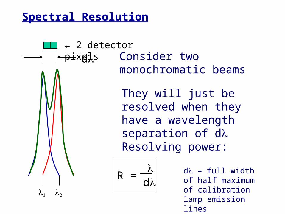
Spectral Resolution
d
1 2
Consider two monochromatic beams
They will just be resolved when they have a wavelength separation of d
Resolving power:
d = full width of half maximum of calibration lamp emission lines
R = d
← 2 detector pixels
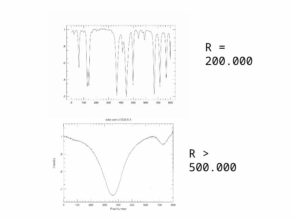
R = 200.000
R > 500.000
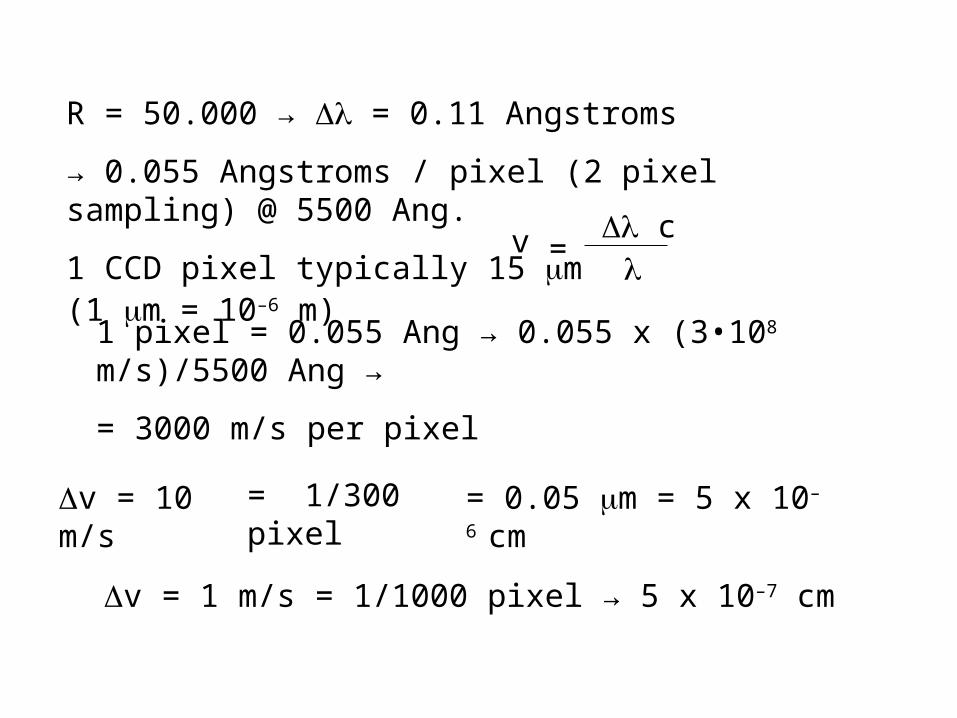
R = 50.000 → = 0.11 Angstroms
→ 0.055 Angstroms / pixel (2 pixel sampling) @ 5500 Ang.
1 CCD pixel typically 15 m (1 m = 10–6 m)
1 pixel = 0.055 Ang → 0.055 x (3•108 m/s)/5500 Ang →
= 3000 m/s per pixel
= v c
v = 10 m/s = 1/300 pixel = 0.05 m = 5 x 10⁻⁶ cm
v = 1 m/s = 1/1000 pixel → 5 x 10⁻⁷ cm
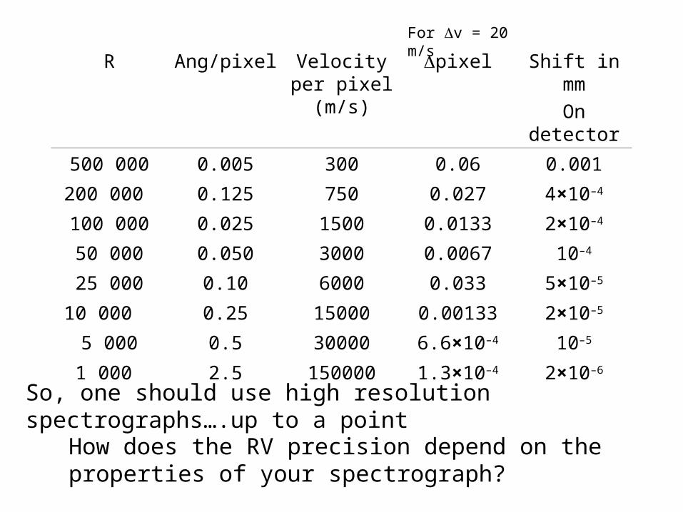
R Ang/pixel Velocity per pixel (m/s)
pixel Shift in mm
On detector
500 000 0.005 300 0.06 0.001
200 000 0.125 750 0.027 4×10⁻⁴
100 000 0.025 1500 0.0133 2×10⁻⁴
50 000 0.050 3000 0.0067 10–4
25 000 0.10 6000 0.033 5×10⁻⁵
10 000 0.25 15000 0.00133 2×10⁻⁵
5 000 0.5 30000 6.6×10⁻⁴ 10–5
1 000 2.5 150000 1.3×10⁻⁴ 2×10⁻⁶
So, one should use high resolution spectrographs….up to a point
For v = 20 m/s
How does the RV precision depend on the properties of your spectrograph?
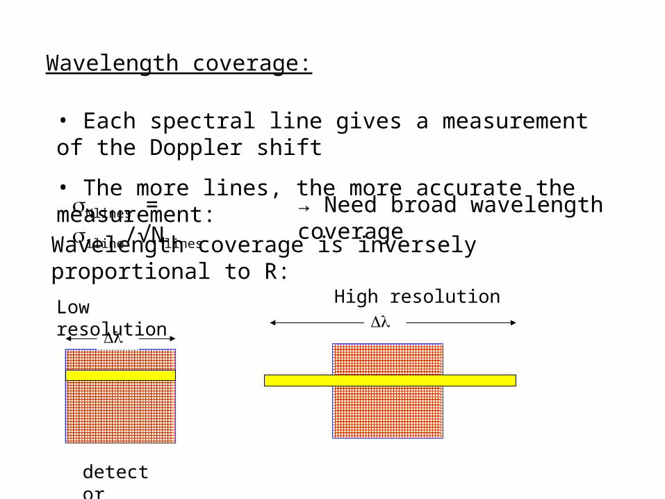
Wavelength coverage:
• Each spectral line gives a measurement of the Doppler shift
• The more lines, the more accurate the measurement:
Nlines = 1line/√Nlines → Need broad wavelength coverage
Wavelength coverage is inversely proportional to R:
detector
Low resolution
High resolution
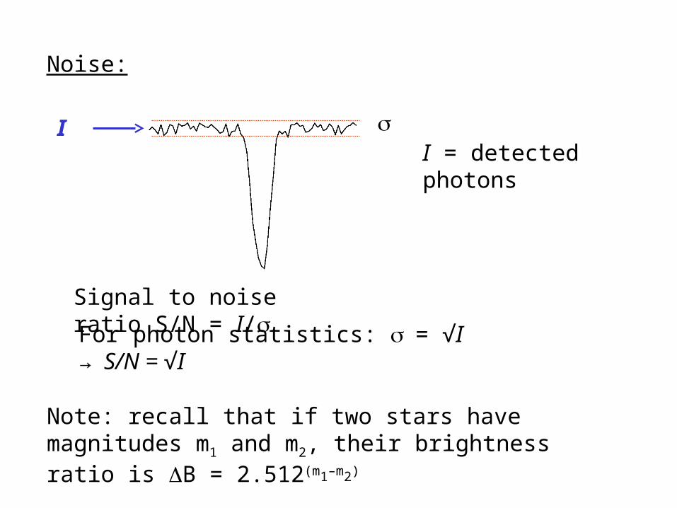
Noise:
Signal to noise ratio S/N = I/
I
For photon statistics: = √I → S/N = √I
I = detected photons
Note: recall that if two stars have magnitudes m1 and m2, their brightness ratio is B = 2.512(m1–m2)
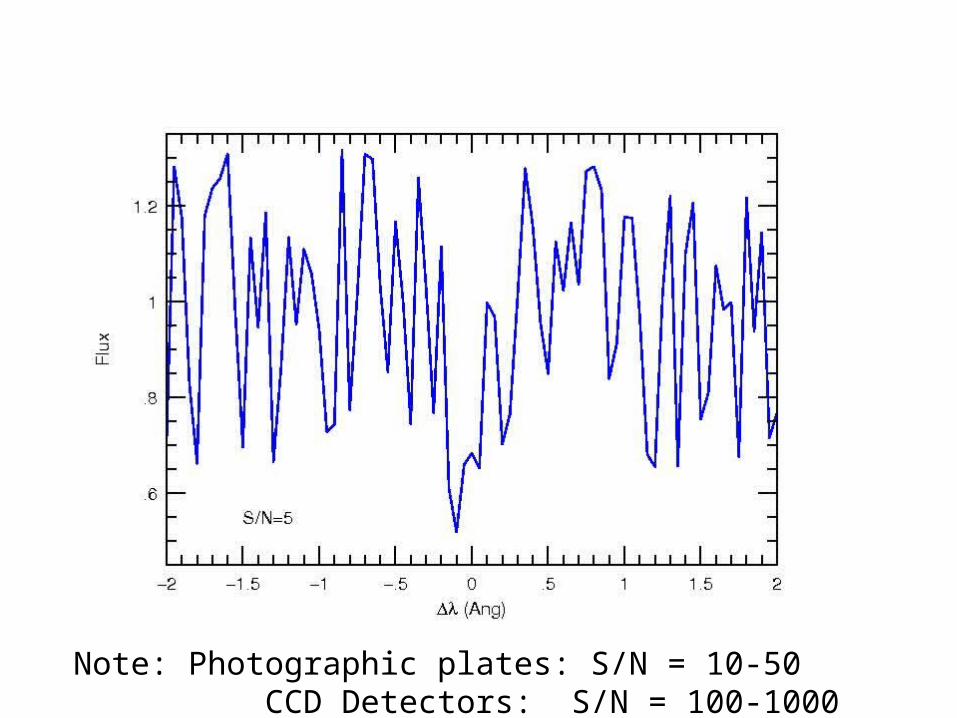
Note: Photographic plates: S/N = 10-50 CCD Detectors: S/N = 100-1000

radialvelocitysimulator.htm
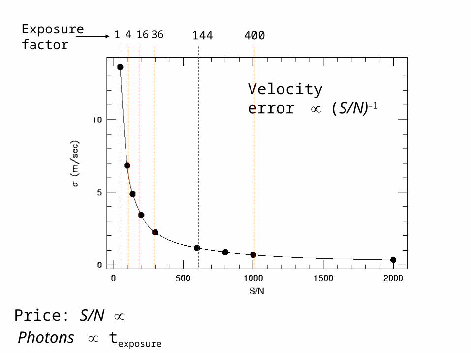
Velocity error(S/N)–
1
Price: S/N t2exposure
1 4Exposure factor
16 36 144 400
Photons texposure
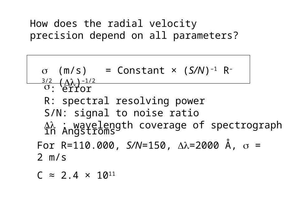
How does the radial velocity precision depend on all parameters?
(m/s) = Constant × (S/N)–1 R–3/2 ()–1/2
: errorR: spectral resolving powerS/N: signal to noise ratio : wavelength coverage of spectrograph in Angstroms
For R=110.000, S/N=150, =2000 Å, = 2 m/s
C ≈ 2.4 × 10¹¹
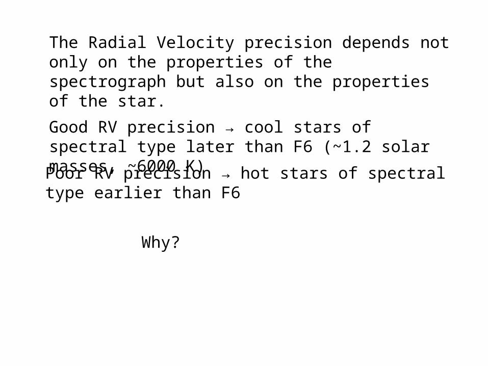
The Radial Velocity precision depends not only on the properties of the spectrograph but also on the properties of the star.
Good RV precision → cool stars of spectral type later than F6 (~1.2 solar masses, ~6000 K)
Poor RV precision → hot stars of spectral type earlier than F6
Why?
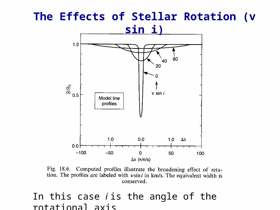
The Effects of Stellar Rotation (v sin i)
In this case i is the angle of the rotational axis
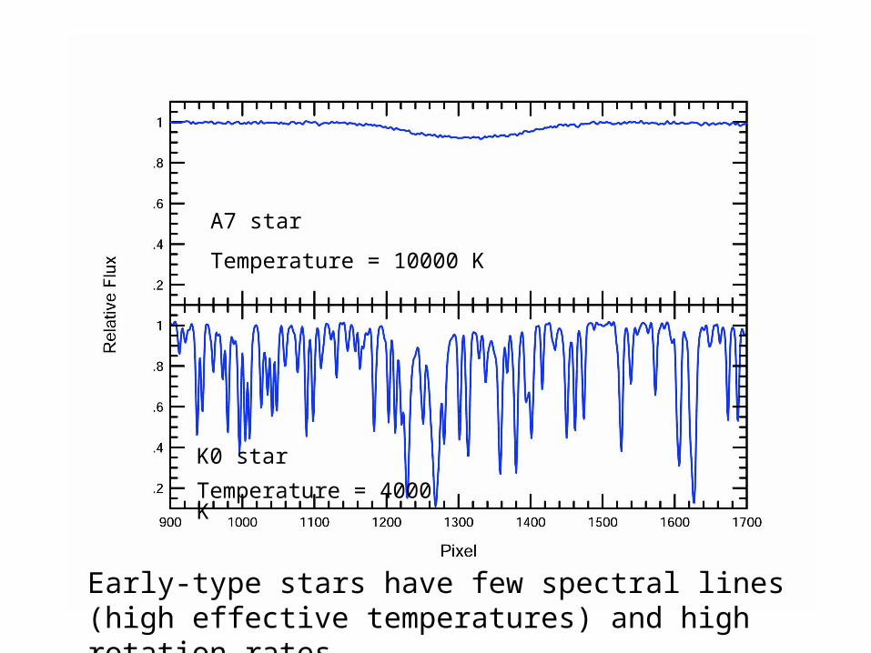
A7 star
Temperature = 10000 K
K0 star
Temperature = 4000 K
Early-type stars have few spectral lines (high effective temperatures) and high rotation rates.
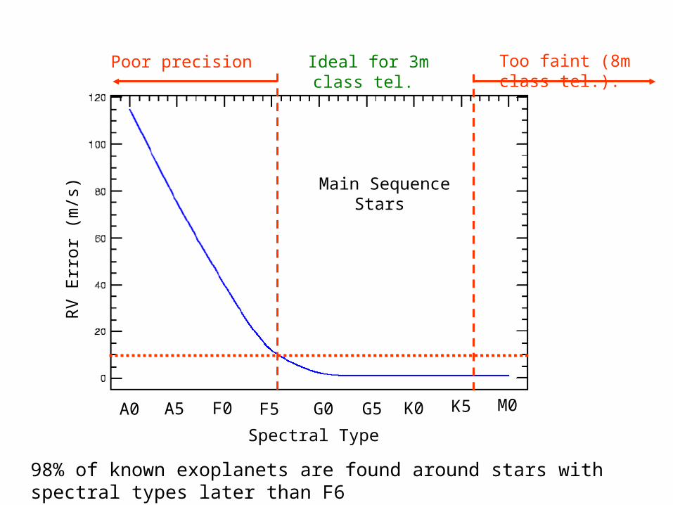
A0 A5 F0 F5
RV
Err
or (
m/s
)
G0 G5 K0 K5 M0
Spectral Type
Main Sequence Stars
Ideal for 3m class tel. Too faint (8m class tel.). Poor precision
98% of known exoplanets are found around stars with spectral types later than F6
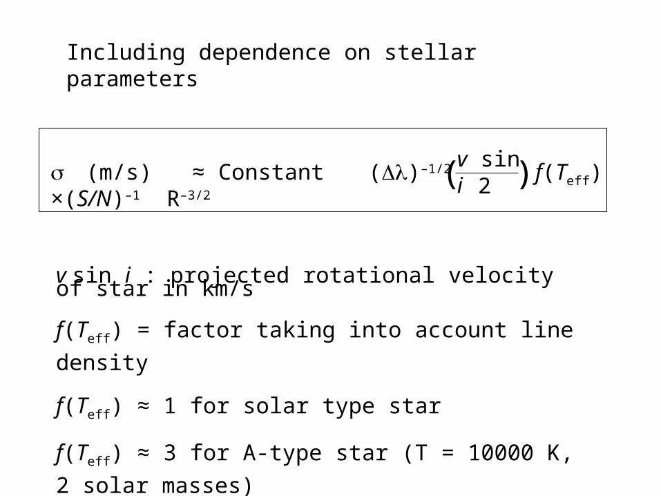
Including dependence on stellar parameters
v sin i : projected rotational velocity of star in km/s
f(Teff) = factor taking into account line density
f(Teff) ≈ 1 for solar type star
f(Teff) ≈ 3 for A-type star (T = 10000 K, 2 solar masses)
f(Teff) ≈ 0.5 for M-type star (T = 3500, 0.1 solar masses)
(m/s) ≈ Constant ×(S/N)–1 R–3/2 v sin i( 2 ) f(Teff)()–1/2
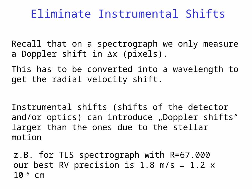
Eliminate Instrumental Shifts
Recall that on a spectrograph we only measure a Doppler shift in x (pixels).
This has to be converted into a wavelength to get the radial velocity shift.
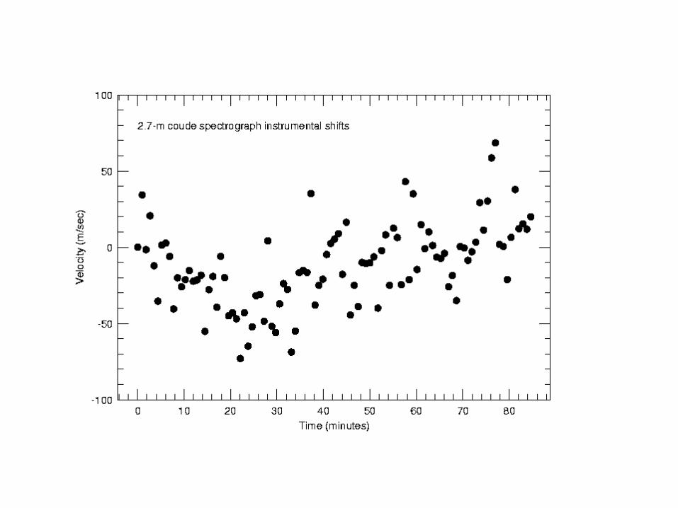
Instrumental shifts (shifts of the detector and/or optics) can introduce „Doppler shifts“ larger than the ones due to the stellar motion
z.B. for TLS spectrograph with R=67.000 our best RV precision is 1.8 m/s → 1.2 x 10⁻⁶ cm
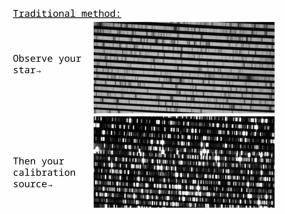
Traditional method:
Observe your star→
Then your calibration source→

Problem: these are not taken at the same time…
... Short term shifts of the spectrograph can limit precision to several hunrdreds of m/s
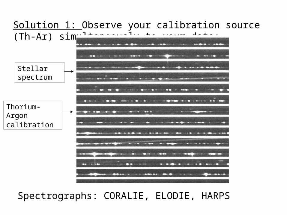
Solution 1: Observe your calibration source (Th-Ar) simultaneously to your data:
Spectrographs: CORALIE, ELODIE, HARPS
Stellar spectrum
Thorium-Argon calibration
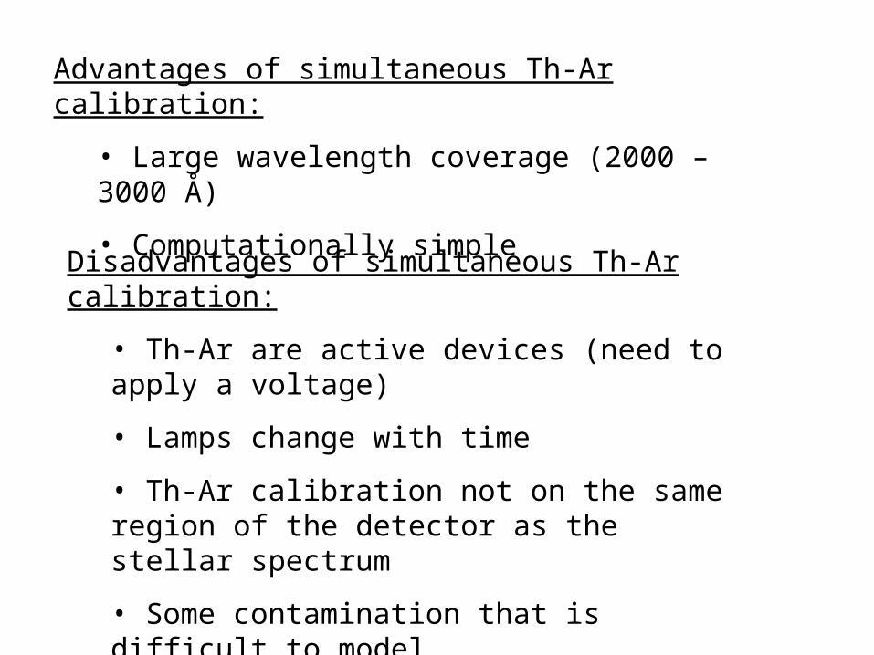
Advantages of simultaneous Th-Ar calibration:
• Large wavelength coverage (2000 – 3000 Å)
• Computationally simple
Disadvantages of simultaneous Th-Ar calibration:
• Th-Ar are active devices (need to apply a voltage)
• Lamps change with time
• Th-Ar calibration not on the same region of the detector as the stellar spectrum
• Some contamination that is difficult to model

One Problem: Th-Ar lamps change with time!
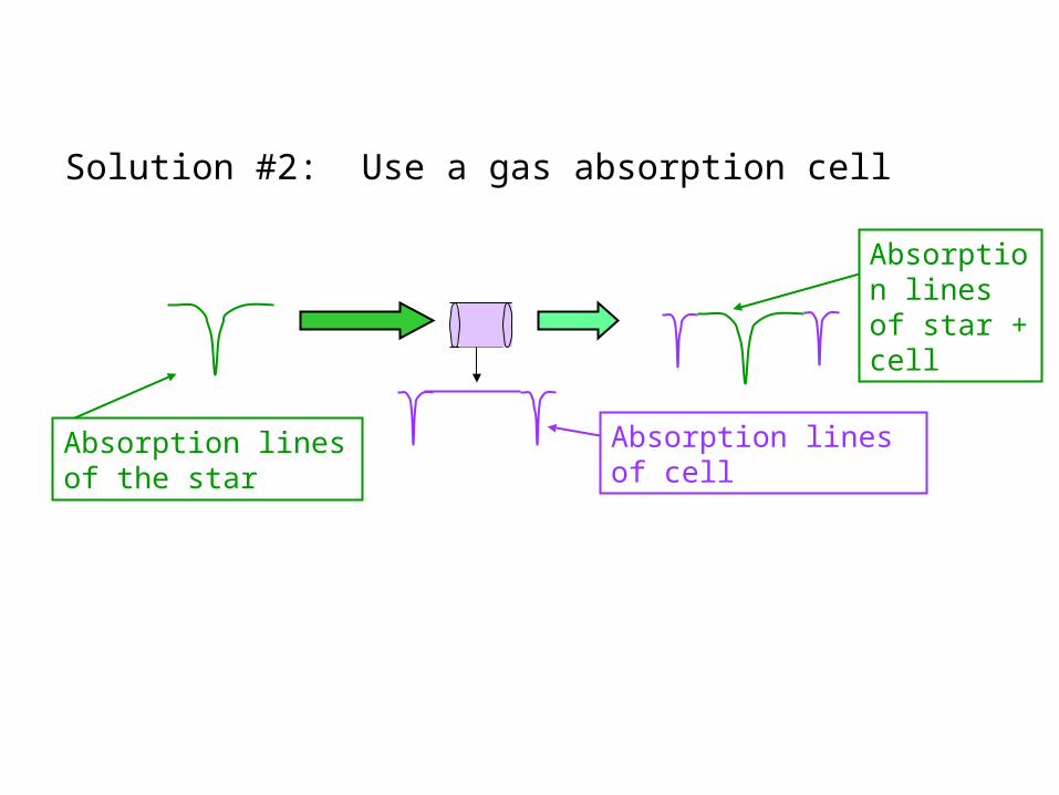
Absorption lines of the star
Absorption lines of cell
Absorption lines of star + cell
Solution #2: Use a gas absorption cell
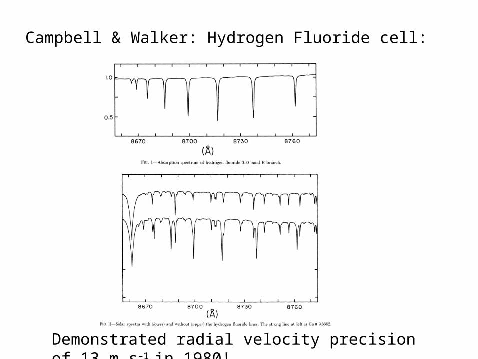
Campbell & Walker: Hydrogen Fluoride cell:
Demonstrated radial velocity precision of 13 m s–1 in 1980!
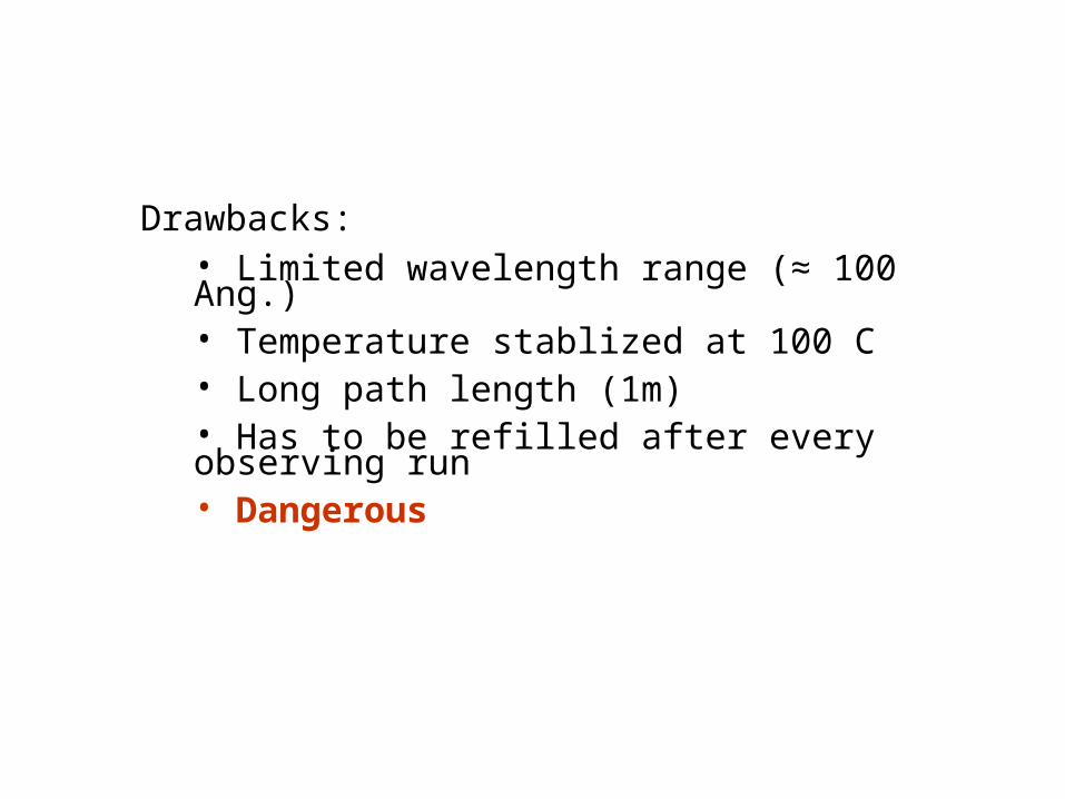
Drawbacks:• Limited wavelength range (≈ 100 Ang.) • Temperature stablized at 100 C• Long path length (1m)• Has to be refilled after every observing run• Dangerous

A better idea: Iodine cell (first proposed by Beckers in 1979 for solar studies)
Advantages over HF:• 1000 Angstroms of coverage• Stablized at 50–75 C• Short path length (≈ 10 cm)• Cell is always sealed and used for >10 years• If cell breaks you will not die!
Spectrum of iodine
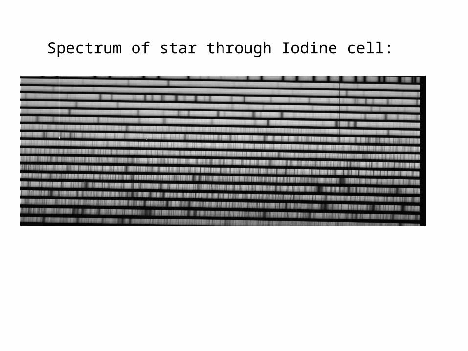
Spectrum of star through Iodine cell:

The iodine cell used at the CES spectrograph at La Silla
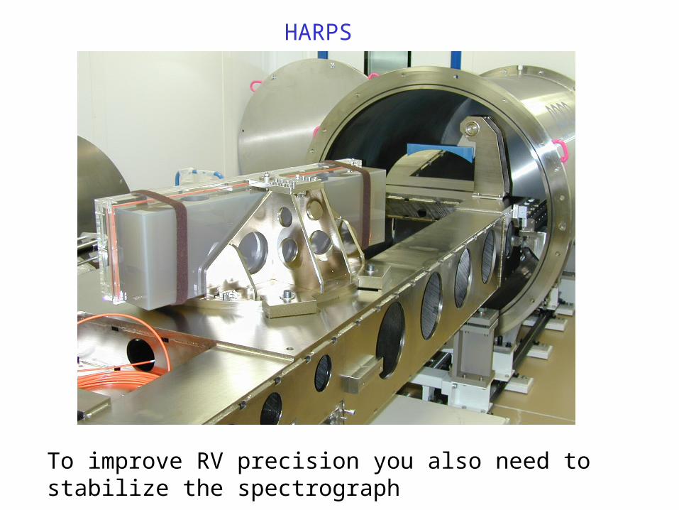
HARPS
To improve RV precision you also need to stabilize the spectrograph
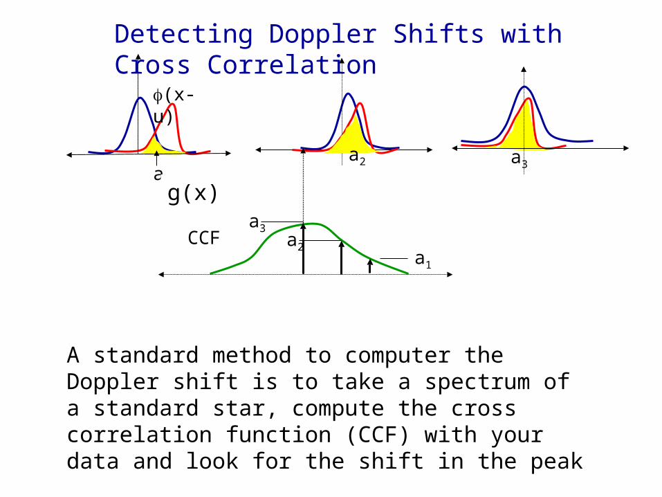
Detecting Doppler Shifts with Cross Correlation
(x-u)
a1
a2
g(x)a3
a2
a3
a1
A standard method to computer the Doppler shift is to take a spectrum of a standard star, compute the cross correlation function (CCF) with your data and look for the shift in the peak
CCF
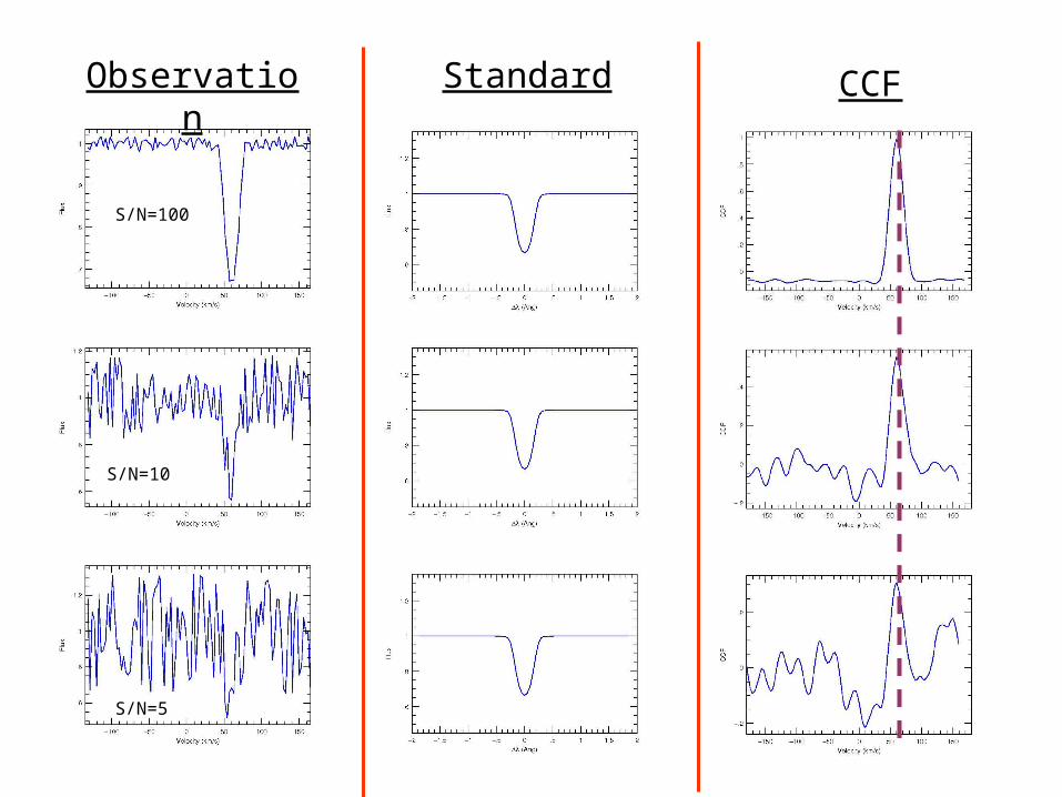
Observation Standard CCF
S/N=100
S/N=10
S/N=5
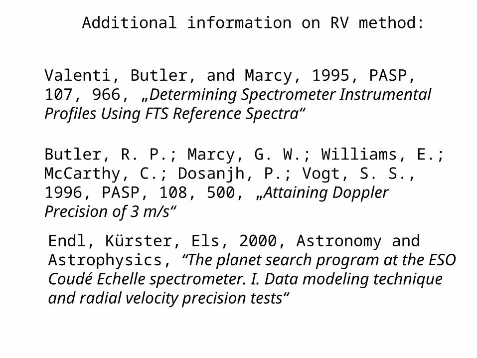
Valenti, Butler, and Marcy, 1995, PASP, 107, 966, „Determining Spectrometer Instrumental Profiles Using FTS Reference Spectra“
Butler, R. P.; Marcy, G. W.; Williams, E.; McCarthy, C.; Dosanjh, P.; Vogt, S. S., 1996, PASP, 108, 500, „Attaining Doppler Precision of 3 m/s“
Endl, Kürster, Els, 2000, Astronomy and Astrophysics, “The planet search program at the ESO Coudé Echelle spectrometer. I. Data modeling technique and radial velocity precision tests“
Additional information on RV method:
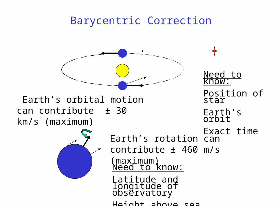
Barycentric Correction
Earth’s orbital motion can contribute ± 30 km/s (maximum)
Need to know:Position of starEarth‘s orbitExact time
Earth’s rotation can contribute ± 460 m/s (maximum)
Need to know:Latitude and longitude of observatoryHeight above sea level
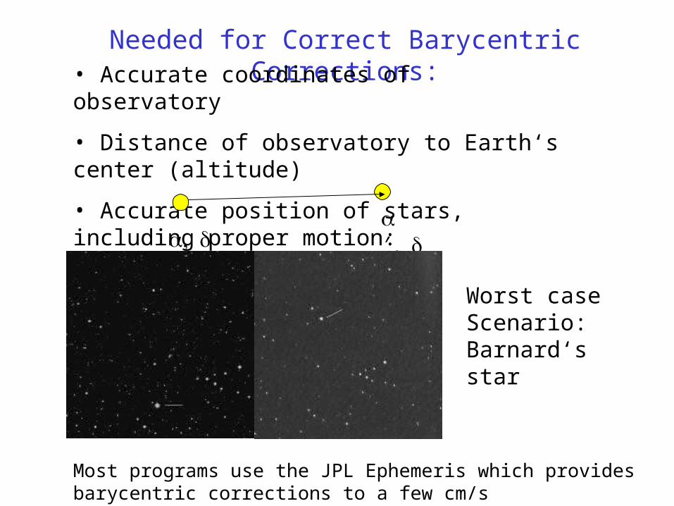
Needed for Correct Barycentric Corrections:• Accurate coordinates of observatory
• Distance of observatory to Earth‘s center (altitude)
• Accurate position of stars, including proper motion:
′′
Worst case Scenario: Barnard‘s star
Most programs use the JPL Ephemeris which provides barycentric corrections to a few cm/s
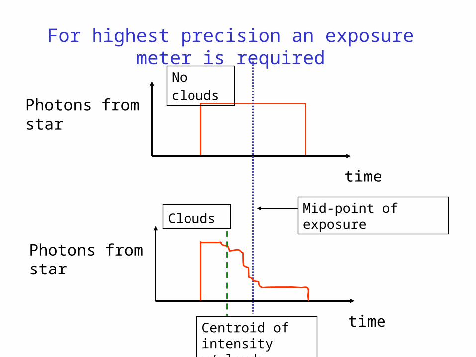
For highest precision an exposure meter is required
time
Photons from star
Mid-point of exposure
No clouds
time
Photons from star
Centroid of intensity w/clouds
Clouds
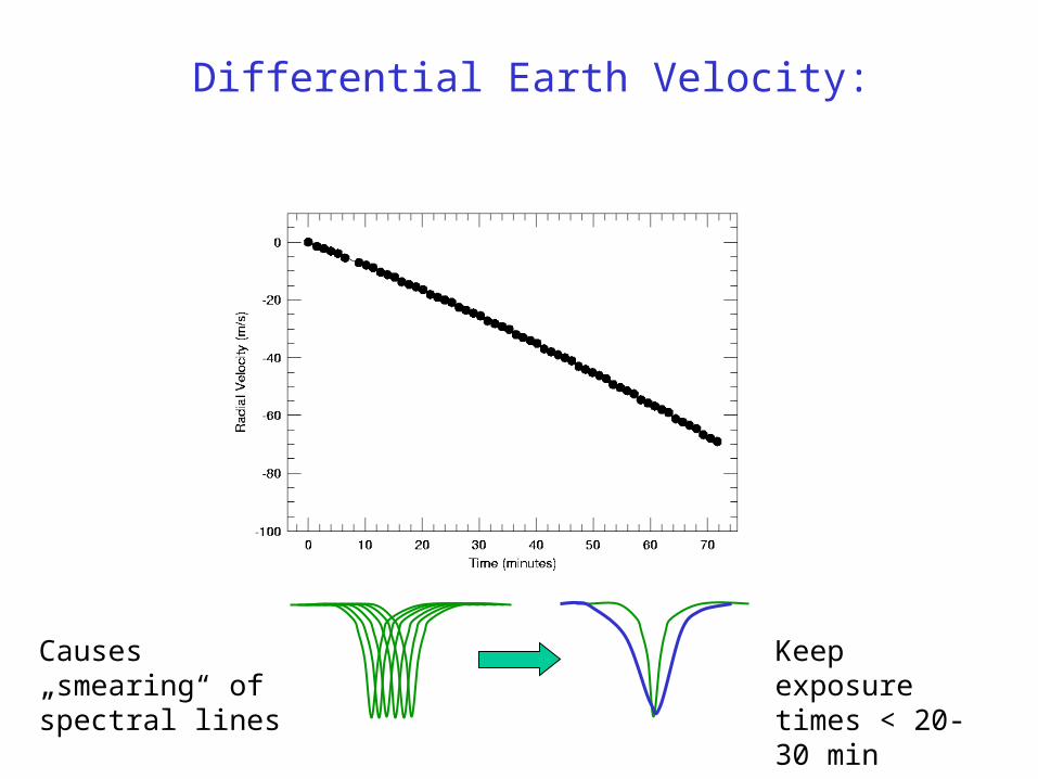
Differential Earth Velocity:
Causes „smearing“ of spectral lines
Keep exposure times < 20-30 min
Finding a Planet in your Radial Velocity Data
1. Determine if there is a periodic signal in your data.
2. Determine if this is a real signal and not due to noise.
3. Determine the nature of the signal, it might not be a planet! (More on this next week)
4. Derive all orbital elements
The first step is to find the period of the planet, otherwise you will never be able to fit an orbit.
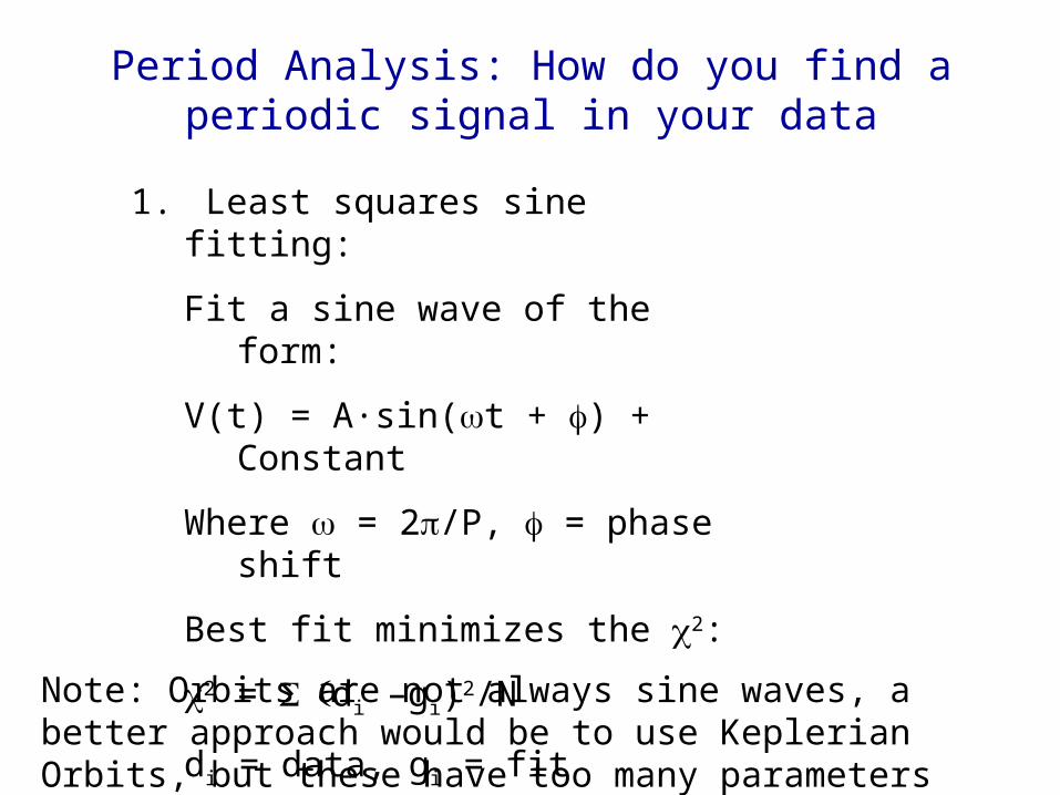
Period Analysis: How do you find a periodic signal in your data
1. Least squares sine fitting:
Fit a sine wave of the form:
V(t) = A·sin(t + ) + Constant
Where = 2/P, = phase shift
Best fit minimizes the 2:
2 = di –gi)2/N
di = data, gi = fit
Note: Orbits are not always sine waves, a better approach would be to use Keplerian Orbits, but these have too many parameters
Period Analysis
2. Discrete Fourier Transform:
Any function can be fit as a sum of sine and cosines
FT() = Xj (T) e–itN0
j=1
A DFT gives you as a function of frequency the amplitude (power = amplitude2) of each sine wave that is in the data
Power: Px() = | FTX()|2
1
N0
Px() =
1
N0
N0 = number of points
[( Xj cos tj + Xj sin tj ) ( ) ]2 2
Recall eit = cos t + i sint
X(t) is the time series
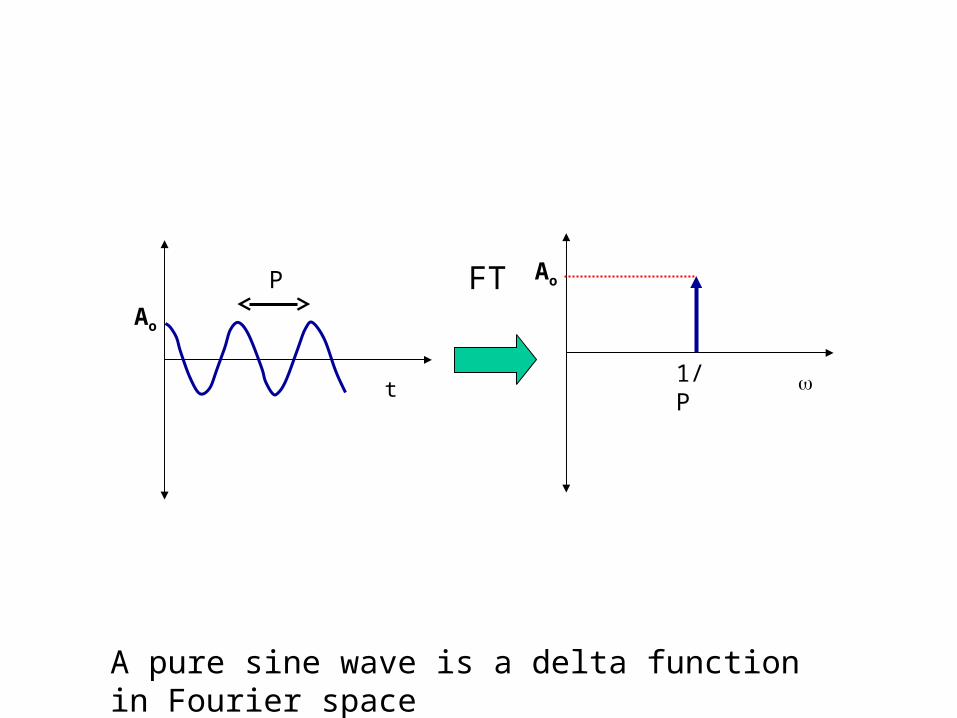
A pure sine wave is a delta function in Fourier space
t
P
Ao
FT
Ao
1/P
Period Analysis
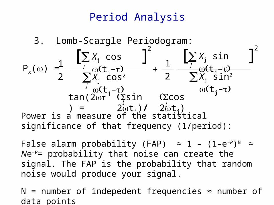
3. Lomb-Scargle Periodogram:
Power is a measure of the statistical significance of that frequency (1/period):
1
2Px() =
[ Xj sin tj–]2
j
Xj sin2 tj–
[ Xj cos tj–]2
j
Xj cos2 tj–j
+1
2
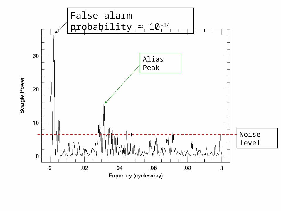
False alarm probability (FAP) ≈ 1 – (1–e–P)N ≈ Ne–P= probability that noise can create the signal. The FAP is the probability that random noise would produce your signal.
N = number of indepedent frequencies ≈ number of data points
tan(2) = sin 2tj)/cos 2tj)j j
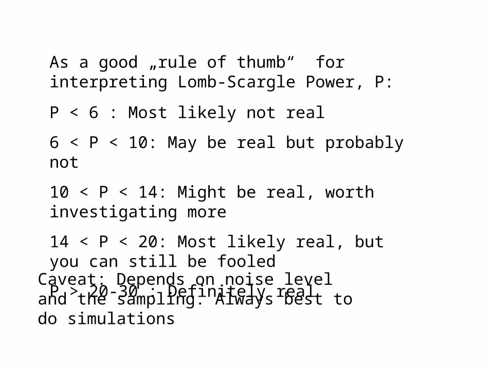
As a good „rule of thumb“ for interpreting Lomb-Scargle Power, P:
P < 6 : Most likely not real
6 < P < 10: May be real but probably not
10 < P < 14: Might be real, worth investigating more
14 < P < 20: Most likely real, but you can still be fooled
P > 20-30 : Definitely real
Caveat: Depends on noise level and the sampling. Always best to do simulations
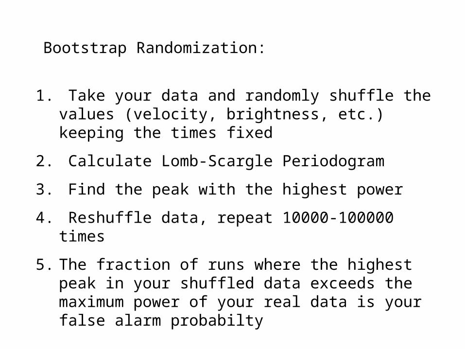
Bootstrap Randomization:
1. Take your data and randomly shuffle the values (velocity, brightness, etc.) keeping the times fixed
2. Calculate Lomb-Scargle Periodogram
3. Find the peak with the highest power
4. Reshuffle data, repeat 10000-100000 times
5. The fraction of runs where the highest peak in your shuffled data exceeds the maximum power of your real data is your false alarm probabilty
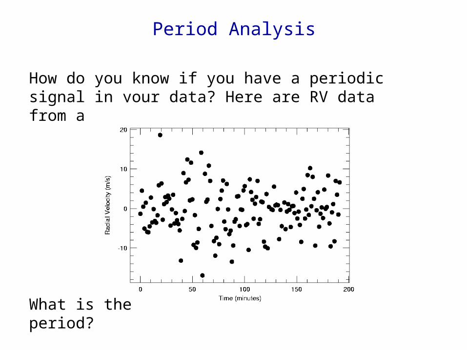
Period Analysis
How do you know if you have a periodic signal in your data? Here are RV data from a pulsating star
What is the period?
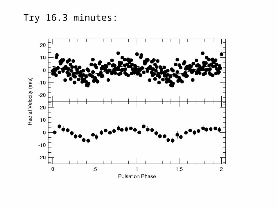
Try 16.3 minutes:
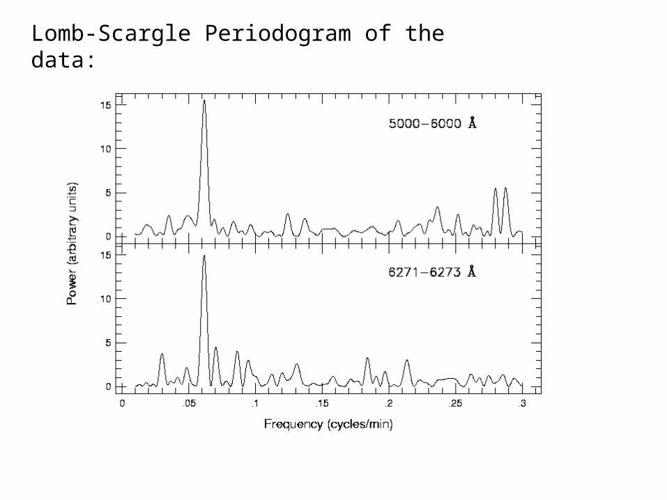
Lomb-Scargle Periodogram of the data:
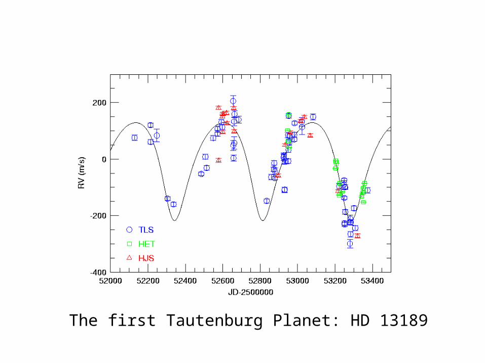
The first Tautenburg Planet: HD 13189
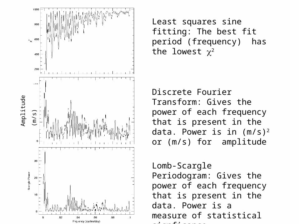
Least squares sine fitting: The best fit period (frequency) has the lowest 2
Discrete Fourier Transform: Gives the power of each frequency that is present in the data. Power is in (m/s)2 or (m/s) for amplitude
Lomb-Scargle Periodogram: Gives the power of each frequency that is present in the data. Power is a measure of statistical signficance
Am
plit
ude
(m/s
)
Noise level
Alias Peak
False alarm probability ≈ 10–14
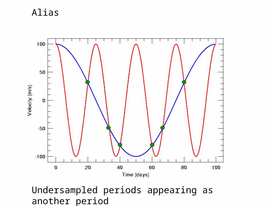
Alias periods:
Undersampled periods appearing as another period
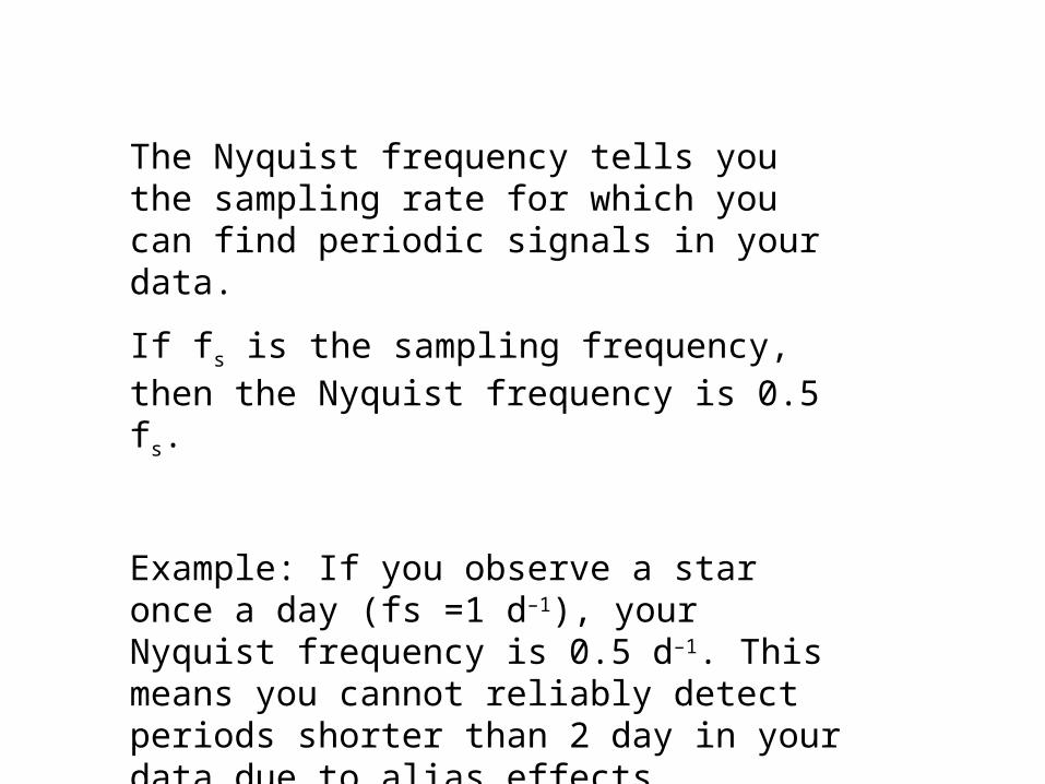
The Nyquist frequency tells you the sampling rate for which you can find periodic signals in your data.
If fs is the sampling frequency, then the Nyquist frequency is 0.5 fs.
Example: If you observe a star once a day (fs =1 d–1), your Nyquist frequency is 0.5 d–1. This means you cannot reliably detect periods shorter than 2 day in your data due to alias effects.
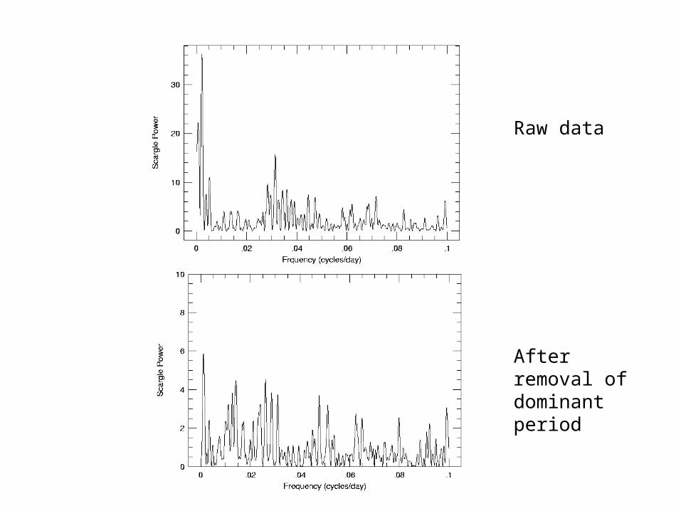
Raw data
After removal of dominant period
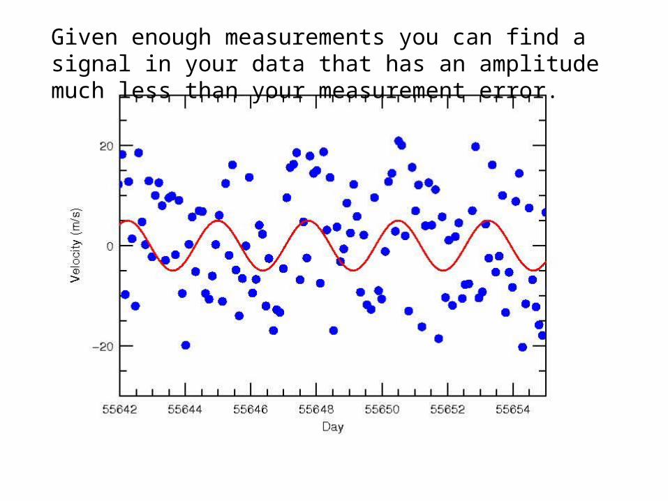
Given enough measurements you can find a signal in your data that has an amplitude much less than your measurement error.
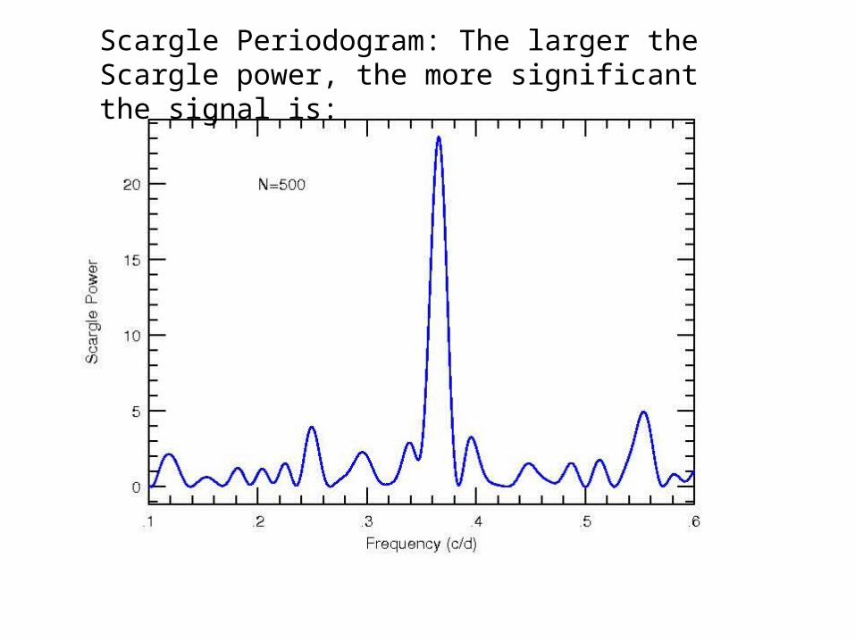
Scargle Periodogram: The larger the Scargle power, the more significant the signal is:
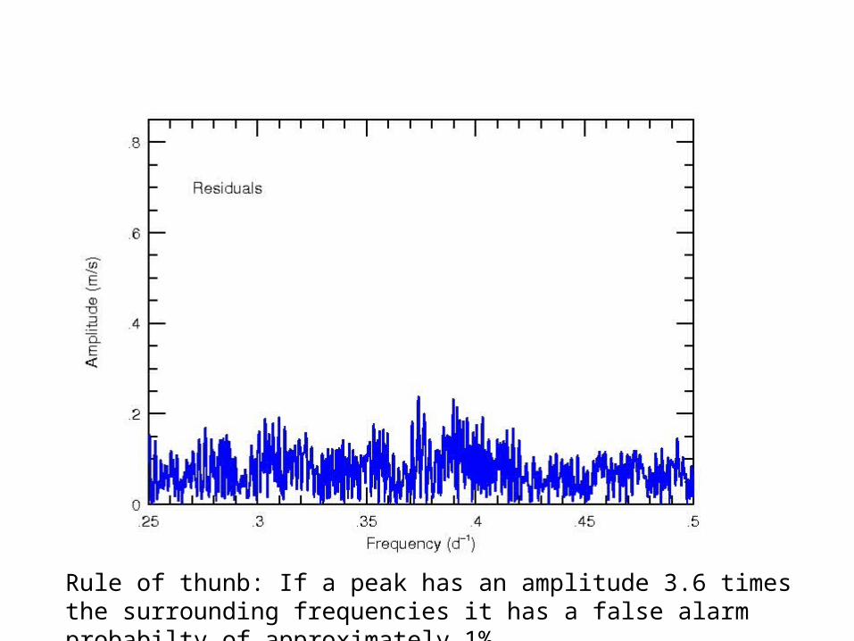
Rule of thunb: If a peak has an amplitude 3.6 times the surrounding frequencies it has a false alarm probabilty of approximately 1%
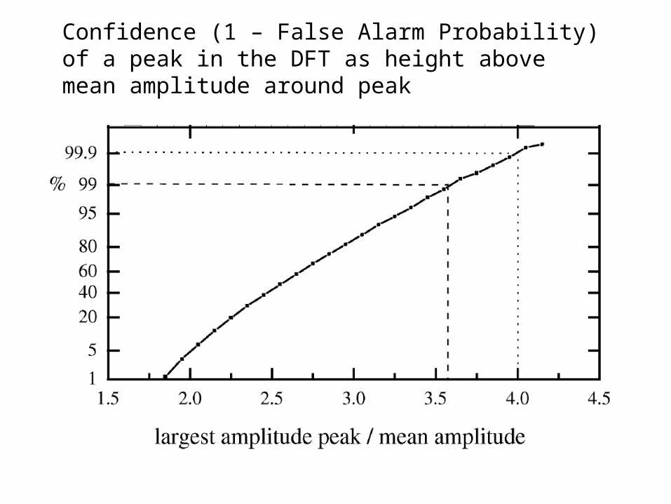
Confidence (1 – False Alarm Probability) of a peak in the DFT as height above mean amplitude around peak
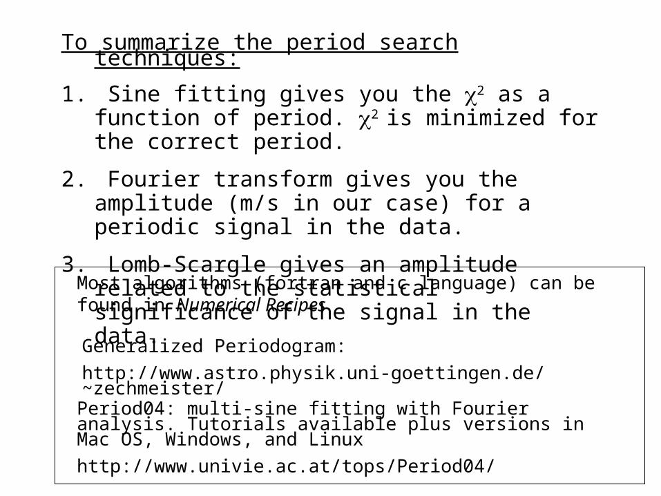
To summarize the period search techniques:
1. Sine fitting gives you the 2 as a function of period. 2 is minimized for the correct period.
2. Fourier transform gives you the amplitude (m/s in our case) for a periodic signal in the data.
3. Lomb-Scargle gives an amplitude related to the statistical significance of the signal in the data.
Most algorithms (fortran and c language) can be found in Numerical Recipes
Period04: multi-sine fitting with Fourier analysis. Tutorials available plus versions in Mac OS, Windows, and Linux
http://www.univie.ac.at/tops/Period04/
Generalized Periodogram:
http://www.astro.physik.uni-goettingen.de/~zechmeister/


