Radial vibration measurements directly from rotors using

laser vibrometry: the effects of surface roughness, instrument

misalignments and pseudo-vibration

Steve J. Rothberg, Ben J. Halkon, Mario Tirabassi and Chris Pusey

Wolfson School of Mechanical and Manufacturing Engineering

Loughborough University, Loughborough, Leicestershire, LE11 3TU, UK.

Corresponding author: Steve Rothberg

e-mail: s.j.rothberg@lboro.ac.uk,

tel: +44 (0) 1509 223440

 

1    

Radial vibration measurements directly from rotors using laser

vibrometry: the effects of surface roughness, instrument

misalignments and pseudo-vibration

Steve J. Rothberg, Ben J. Halkon, Mario Tirabassi and Chris Pusey

Wolfson School of Mechanical and Manufacturing Engineering

Loughborough University, UK

Abstract: Laser Doppler vibrometry (LDV) offers an attractive solution when radial vibration measurement directly from a rotor surface is required. Research to date has demonstrated application on polished-circular rotors and rotors coated with retro-reflective tape. In the latter case, however, a significant cross-sensitivity to the orthogonal radial vibration component occurs and post-processing is required to resolve individual radial vibration components. Until now, the fundamentally different behaviour observed between these cases has stood as an inconsistency in the published literature, symptomatic of the need to understand the effect of surface roughness. This paper offers the first consistent mathematical description of the polished-circular and rough rotor behaviours, combined with an experimental investigation of the relationship between surface roughness and cross-sensitivity. Rotors with surface roughness up to 10 nm satisfy the polished-circular rotor definition if vibration displacement is below 100% beam diameter, for a 90 µm beam, and below 40% beam diameter, for a 520 µm beam. On rotors with roughness between 10 nm and 50 nm, the polished-circular rotor definition is satisfied for vibration displacements up to 25% beam diameter, for a 90 µm beam, and up to 10% beam diameter, for a 520 µm beam. As roughness increases, cross-sensitivity increases but only rotors coated in retro-reflective tape satisfied the rough rotor definition fully. Consequently, when polished-circular surfaces are not available, rotor surfaces must be treated with retro-reflective tape and measurements post-processed to resolve individual vibration components. Through simulations, the value of the resolution and correction algorithms that form the post-processor has been demonstrated quantitatively. Simulations incorporating representative instrument misalignments and measurement noise have enabled quantification of likely error levels in radial vibration measurements. On a polished-circular rotor, errors around 0.2% for amplitude and 2 mrad for phase are likely, rising a little at the integer orders affected by pseudo-vibration. Higher pseudo-vibration levels and the need for resolution increase errors in the rough rotor measurements, especially around the synchronous frequency where errors reach 20% by amplitude and 100 mrad for phase. Outside a range of half an order either side of first order, errors are ten times lower and beyond fifth order errors are similar to those for the polished-circular rotor. Further simulations were performed to estimate sensitivities to axial vibration, speed variation and bending vibrations.  KEYWORDS: Laser vibrometry, radial, rotor, vibration measurement, surface roughness, misalignment, pseudo-vibration.

2    

1. Introduction

Vibration is readily acknowledged as the most effective measure of the condition of rotating

machines. Such vibrations are inevitable but their consequences can be dramatic, extending from loss

of efficiency through to safety-critical failures. There are also the associated issues of noise generation

and user discomfort which can, for example, affect perceptions of product quality and adherence to

legislative requirements. Monitoring techniques are mature; the earliest significant attempts to

quantify acceptable machinery vibration levels date from the late 1930s [1] and the value of vibration

analysis in the diagnosis of machine health is regularly reiterated in the published literature e.g. [2-

14].

Transducer selection first involves consideration of whether to measure displacement, velocity or

acceleration. Vibration velocity is generally regarded as the optimum measurement parameter but

traditional velocity transducers cannot match the dynamic range and frequency range of the

ubiquitous piezo-electric accelerometer, even after integration of the measured signal [2]. In addition,

choice must be made between measurement of shaft absolute vibration, shaft vibration relative to

bearings or housing absolute vibration (usually taken at bearing locations) [3]. Measurement of any

two of these options allows derivation of the third and this requirement is typically met via proximity

probes (generally eddy current based) for the second option and piezo-electric accelerometers for the

third option.

This paper is concerned with the application of laser Doppler vibrometry (LDV) to the monitoring of

rotating machinery. Laser vibrometers are now well established as an effective alternative to more

traditional vibration transducers. For the application in question, they offer direct measurement of the

favoured parameter (i.e. velocity) with dynamic and frequency ranges at least matching and generally

exceeding those offered by piezo-electric accelerometers. Measurements from non-rotating parts are

straightforward, provided optical access is available, with particular advantages where the context

demands high frequency operation or remote transducer operation, or when the structure itself is hot

or light. Most importantly, they also offer the opportunity to measure directly from rotating parts. This

is not a new realisation; since the appearance of commercial instruments in the 1980s, measurements

directly from rotating targets have been regularly highlighted by manufacturers and researchers as a

major application area. LDV applications for axial vibration measurement directly from rotating

blades date back over 40 years [15] and interest in similar applications continues today using both

stationary [16] and scanning [17] laser beams. Radial, torsional and bending vibration measurements

have also been successfully demonstrated [18].

Radial vibration measurements are the specific focus of this paper. Applications of particular interest

include automotive powertrain [18], hard disks and their drive spindles [19, 20] and tool condition

monitoring in turning [21] and milling [22, 23]. Similar measurement configurations have revealed

3    

details related to shaft rotation [24, 25]. Early attempts to use LDV for radial vibration measurements

on rotors, however, identified a cross-sensitivity to the radial vibration component perpendicular to

the radial component it is intended to measure. This cross-sensitivity was shown to be a consequence

of oscillation in the position of the rotor centre relative to the fixed line of incidence of the beam [26].

The finding prompted development of a model to predict measured velocity for arbitrary beam

orientation and arbitrary target motion [27] ultimately resulting in confirmation that this cross-

sensitivity could not be resolved by laser beam orientation alone. A resolution procedure based on

three simultaneous measurements was subsequently formulated [28].

These cross-sensitivity studies had concentrated on rotating surfaces treated with retro-reflective tape

(Scotchlite high-gain sheeting type 7610), a common surface treatment intended to maximise the

intensity of light scattered back towards the instrument’s collecting optics. In a separate study [29],

vibration measurements on a painted rotor confirmed the presence of this cross-sensitivity but

measurements made on a polished rotor (Ra 20 nm) showed no such cross-sensitivity. Resolution of

this inconsistency is one of the main novelties of this paper. An initial study [30] has highlighted the

dependence of the extent of the cross-sensitivity in radial vibration measurements on not just surface

roughness but also on incident laser beam diameter, emphasising the urgent need for a thorough study.

Having identified the surface conditions under which radial vibration measurements can be made, this

paper then proceeds to use simulation to estimate the errors likely in real measurements as a result of

i) inevitable instrument misalignment (relative to rotor axes), ii) other motion components and iii)

measurement noise. Incorporation of these aspects into simulations is enabled by two important recent

developments. The study of misalignments and sensitivity to other motion components is facilitated

by a new, vectorial framework for modelling measured velocity in laser vibrometry [31] while the

inclusion of measurement noise is enabled by the recent quantification of pseudo-vibration

sensitivities as a function of surface roughness or treatment for a range of commercial laser

vibrometers [32, 33]. Further novelty in this paper lies in this application of the modelling framework

and its combination with the pseudo-vibration study.

2. Modelling the Measured Velocity

Watrasiewicz and Rudd [34] captured the fundamental relationship between measured velocity, mU ,

and surface velocity at a point P, PV , in the expression:

( ) Pinoutm VbbU ⋅−= ˆˆ21

(1)

4    

in which inb and outb are unit vectors for the incoming and outgoing laser beam directions,

respectively. When the light is collected from the target surface in direct backscatter, as is typical in

commercial laser vibrometers, then outin bb ˆˆ −= and equation (1) simplifies to:

Pinm VbU ⋅−= ˆ (2)

This expression highlights the attraction of a model based on vector descriptions of both surface

velocity and beam direction [31]. Arbitrary beam orientation can be incorporated into a unit vector for

beam direction while six degree-of-freedom vibration of the illuminated target element, together with

any continuous motion such as the whole body rotation of interest here, can be incorporated into the

surface velocity vector to enable a comprehensive analysis of measured velocity. The analysis

presented here, up to the end of sub-section 2.1, refreshes an earlier analysis [27] by adopting the

vector based approach now recommended. This approach is necessary to enable the analysis of

misalignment errors in section 5. It also serves as an introduction to the wholly new analysis for the

polished-circular rotor in section 2.2.

For laser beam orientation, consider an initial alignment of the incoming laser beam such that

xbin ˆˆ =− , as shown in figure 1. This initial orientation is an arbitrary choice but is made for

consistency with earlier analysis [27] as is the order of the rotations resulting in the arbitrary direction

of incidence. A first rotation by β around the y-axis and a second rotation by γ around the z-axis are

accommodated using the rotation matrices [ ]β,y and [ ]γ,z to provide the following expression for

beam orientation:

[ ][ ][ ][ ] [ ][ ]TTin zyxyzzyxb βγβγββγ sinsincoscoscosˆˆˆ001,,ˆˆˆˆ −==− (3)

Rotation matrices are used at several stages in this paper and they are shown in Appendix A.

Surface velocity at any point P on the target is most conveniently written in terms of the sum of a

translational velocity, *OV , of origin O*, which is fixed within the structure, and the velocity of P

relative to O* as a result of rotation, about an instantaneous rotation axis passing through O*, at

angular velocity ω

:

POVV OP ** ×+= ω

(4)

where PO* is the vector from O* to P. In the analysis that follows, O* on the structure sits at O, the

origin of the global coordinate system, in the absence of vibration. Consequently, vector *OO is the

5    

vibration displacement of that point. Figure 2a shows this arrangement in which the rotor centre has

displaced from O to O*. Equation (4) does assume that the small element of the shaft illuminated by

the laser beam can be considered rigid. If this assumption cannot be made then velocity associated

with the flexible component of vibration can be added in vector form to equation (4).

2.1 The rough rotor model

Figure 2a shows the illuminated region on a displaced rotor together with two individual rays within

the laser beam. The upper ray follows the laser beam centre-line; this is the line associated with laser

beam incidence when the finite size of the laser beam is ignored and is the basis of the analysis in this

sub-section. When the rotor surface is rough (surface roughness at least comparable with the laser

wavelength), the scattering of light is diffuse; light from a uniform intensity laser beam would arrive

at the photodetector from all parts of the beam with equal probability. For the Gaussian beam, light

collection is influenced by the intensity envelope of the beam and, relative to a uniform intensity

beam, this makes the assumption that the dominant collected light intensity originates from the

geometric centre of the beam even more reasonable. Consequently, the case considered in this sub-

section is termed ‘the rough rotor model’.

The figure shows how the incident point P will change continuously as a result of vibration,

compounded by any shaft out-of-roundness. This change may be difficult or at least inconvenient to

predict and this would seem to be problematic in terms of progressing this analysis from equation (4).

This apparent obstacle is, however, readily overcome. No matter how the specific point of incidence

on the shaft moves, that point of incidence will always lie somewhere along the line of the beam. Any

point on the line of the beam can be described as the sum of the position vector of a single (but

arbitrary) known point 0r that lies on the beam and a multiple of the unit vector defining the direction

of the beam. Significant points of interest are shown more clearly in Figure 2b. At any time, t, the

instantaneous point of incidence can always be written as:

( ) inbtpOOrPO ˆ** 0 +−= (5a)

where the distance ( )tp is generally unknown and

[ ][ ]Tzyxzyxr 0000 ˆˆˆ= (5b)

Substituting equations (4) and (5a) into equation (2) gives:

( )( ) ( )( )ininOinm btpbOOrVbU ˆˆ*ˆ0* ×⋅−−×+⋅−= ωω

(6)

6    

The second scalar triple product in equation (6) is always zero [27] and so the introduction of vector

0r was a significant step. It showed that prediction of measured velocity only requires knowledge of

any one point along the beam rather than the specific and continuously changing point of incidence on

the target. At the same time and in the most general sense, the analysis confirms, by the elimination of

( )tp from equation (6), the important shape insensitivity associated with vibrometer measurements

on a rough rotor. The rough rotor model is, therefore, based on the following description of the

measured velocity:

( )( )*ˆ0* OOrVbU Oinm −×+⋅−= ω

(7)

The angular velocity vector, ω

, includes both angular vibration velocities around the three coordinate

axes, [ ]Tzyx θθθ , and the continuous target rotation at angular frequency Ω . This continuous

rotation occurs around an axis, defined by unit vector Rz as shown in Figure 2b, that is itself affected

by the angular oscillations of the target. This is written in terms of an initial z-orientation modified by

pitch and yaw vibration displacements, enabling a full expression for angular velocity to be written as:

Rz' Ω+=ωω

(8a)

in which

[ ][ ]Tzyxzyx θθθω ˆˆˆ' = (8b)

and

[ ][ ][ ][ ]TxyR xyzyxz 100,,ˆˆˆˆ θθ= (8c)

The origin of the cross-sensitivity in the rough rotor measurements lies in the term RzΩ . Full

expansion of equation (7), as presented in Appendix B, and its original experimental validation [27]

confirmed the presence of this cross-sensitivity and showed that its resolution could not be achieved

by beam manipulation or other simple means. The significance of beam orientation in isolating the so-

called ‘vibration sets’ was also highlighted. Isolation of the x-radial and y-radial vibration sets

requires laser beam alignment with xbin ˆˆ =− , 00 =r and ybin ˆˆ =− , 00 =r , respectively. Neglecting

smaller terms, the respective velocity measurements mxU and myU are written as:

yxU totmx Ω+= (9a)

7    

xyU totmy Ω−= (9b)

in which Ω+=Ω ztot θ . In equation (9a), for example, the desired measurement is of the x-radial

velocity but there is a significant sensitivity to y-radial displacement. Equations (9a&b) therefore

show, in the simplest terms, the cross-sensitivity encountered in radial vibration measurements on a

rough rotor i.e. when 0≠Ω .

2.2 The polished-circular rotor model

The foregoing analysis quite reasonably assumed that light collected had originated from the

geometric centre of the Gaussian laser beam. Of course, the laser beam has finite size and light is

scattered from all parts of the illuminated region on the target for collection through the vibrometer

aperture. In a measurement from a polished-circular rotor, there will be a tendency for incident light

to be reflected away from the vibrometer’s collecting aperture if it is incident away from a line

passing directly through the centre of rotation. Figure 3 shows how light incident along a line through

the rotation centre is preferentially collected, representing a shift in the effective centre of the laser

beam away from the geometric centre.

Figures 2a&b show a second ray within the incident laser beam, incident on the displaced rotor

(radius R) at point P’. This ray intersects the rotor centre-line at point Q and, for a polished-circular

rotor, it represents the part of the incident laser beam that instantaneously dominates the collected

light intensity. The same approach as that used in section 2.1 can be taken to predict the measured

velocity. Consider the vector triangle O*P’Q shown in Figure 2b:

( ) inR bRztqQPQOPO ˆˆ'*'* −=+= (10)

where the distance ( )tq is generally unknown. Combination of equations (2), (4), (8a) and (10) for

the point P’ gives:

( ) ( )( )( )inRROinm bRztqzVbU ˆˆˆ'ˆ* −×Ω++⋅−= ω (11)

Expansion of equation (11) leads to elimination of the vector term inbR ˆ , in the same way as for the

second term of equation (6). Elimination of RzΩ from the cross product then occurs as follows:

( ) ( )( ) ( )( )ROinRROinm ztqVbztqzVbU ˆ'ˆˆˆ'ˆ** ×+⋅−=×Ω++⋅−= ωω (12)

This significant step shows how the polished-circular rotor measurement loses its dependence on

rotation speed, Ω , eliminating the cross-sensitivity that is so problematic in the rough rotor

8    

measurement. The effective centre-line of the beam (from which the dominant contribution to

collected light intensity instantaneously originates) passes through a point defined by the sum of the

position vectors 0r and ( )tr0Δ , as shown in Figure 2b. As in the rough rotor model, 0r is the position

vector for the geometric centre-line of the laser beam while ( )tr0Δ is the vector from this point to

another (arbitrary) chosen position along the instantaneous effective centre-line of the beam. Its time

dependency is a result of the vibrations of the polished-circular rotor. These vectors are related to each

other as follows:

( ) ( ) ( )( ) *ˆ'*ˆ 00 OObRtptrrQOztq inR −++Δ+== (13)

where the distance ( )tp' is generally unknown. On substitution into equation (12), the term related to

beam orientation in equation (13) is once again eliminated and the measured velocity takes a similar

form to equation (7):

( ) ( )( ) ( )( )*'ˆ'*'ˆ0*00* OOrVbtrOOrVbU OinOinm −×+⋅−≈Δ×+−×+⋅−= ωωω (14)

The vector ( )tr0Δ is difficult to obtain. In reality, of course, a single point does not exist and an

extended region of the incident beam will intersect the rotor axis and contribute to measured velocity.

Additionally, in a focussed beam, orientation varies slightly across the beam. Nonetheless, this simple

presentation, delivered here for the first time, neatly captures the fundamentals of the polished-

circular rotor measurement. The approximation simplifying equation (14) is based on the reasonable

assumption that, in this application, the effective centre of the Gaussian laser beam will always lie

close to its geometric centre and later simulations for the polished-circular rotor are based on this

approximate expression.

3. The effect of surface roughness and treatment on cross-sensitivity

In terms of the effective centre-line of the laser beam, a transition might be expected from the line

following the geometric centre of the laser beam for a rough rotor to a (nearly) parallel line passing

through the rotor centre for a polished-circular rotor. A critically important and very practical question

thus emerges. What values of surface roughness or what types of surface treatment will result in

measurements conforming to either the rough rotor model or the polished-circular rotor model? In

addition, what will be the effects of factors such as rotor out-of-roundness, vibration amplitude and

incident beam diameter?

9    

3.1 Experimental investigation

With constant rotation speed and vibration at angular frequency vω applied in the x-radial direction

only, frequency domain representations of equations (9a&b) might be written:

[ ] [ ]vv

xFTUFT mx ωω= (15a)

[ ] [ ] [ ]vvv

xjFTxFTUFTv

tottotmy ωωω ω

Ω=Ω−= (15b)

where [ ]v

FT ω signifies the Fourier transform evaluated at frequency vω . A “cross-sensitivity ratio”

can be formed based on an estimate of x-radial velocity from myU and the mxU measurement itself as

follows:

[ ][ ]

v

v

mx

my

tot

v

UFT

UFTR

ω

ωωΩ

=100 (16)

Radial vibration measurements on rotors with their surface coated with retro-reflective tape have been

investigated extensively [26, 27, 30] and these will return a ratio of 100%, in accordance with the

theory presented in section 2.1.1. Measurements without cross-sensitivity, such as those reported on a

polished-circular rotor [29], would return a ratio of zero. Both conditions are repeated in the

experimentation presented here but, of particular interest, is how the ratio varies with surface

roughness and for other surface treatments.

As shown in Figure 4a, a small, unloaded test rotor is driven by an electric motor through a flexible

belt such that the rotor exhibits minimal self-induced vibration. The whole system is mounted on a

linear bearing and a controlled vibration is introduced along a single radial direction by an

electromagnetic shaker. This direction is defined to be the x-direction while the rotor spin axis defines

the z-direction. The alignment between the laser beams and rotor is shown in Figure 4b. A laser

vibrometer is aligned in the x-radial direction with misalignments minimised i.e. xbin ˆˆ ≈− , 00 ≈r , to

make the measurement of genuine motion described by equation (15a). A second laser vibrometer is

aligned in the y-direction with misalignments minimised such that ybin ˆˆ ≈− , 00 ≈r . The genuine

motion in this direction is (nominally) zero and so any velocity measured is a consequence of cross-

sensitivity as described by equation (15b). From these measurements, cross-sensitivity ratio is

calculated for each test set-up.

10    

The rotor bearing caps can be removed to allow the test rotor to be changed without disturbing the

vibrometer alignments. The various test rotors have diameter 15 mm, length 30 mm and roughness

values in a range between Ra 10 nm and Ra 1100 nm, as shown in Table 1. Out-of-roundness was

simply intended to be as small as possible. Measurements were also made on surfaces treated with

retro-reflective tape and with white paint. Tests were conducted for a number of combinations of

rotation frequency (up to 25 Hz), vibration frequency (up to 87.5 Hz) and vibration velocity (generally

from 5 mm/ s to 100 mm/s) and these are intended to be representative of real measurements.

Vibration frequencies were always half way between integer multiples of rotation frequency to avoid

pseudo-vibration which is concentrated at integer multiples of rotation speed [33].

In order to investigate the effect of incident laser beam diameter, the cross-sensitivity ratios were

calculated for measurements taken with two different vibrometers making the y-radial measurement.

The Polytec OFV323 has an incident beam diameter of 90 µm (stand-off distance 600 mm) while the

Polytec OFV400 (used here in the single beam mode with stand-off distance 400 mm) has an incident

beam diameter of 520 µm. In all tests, the x-radial measurement was made by a Polytec OFV303 with

beam diameter 90 µm at a stand-off distance of 600 mm.

3.2 Cross-sensitivity: analysis of mean ratios

A summary of the measured cross-sensitivity ratios, together with corresponding roughness and out-

of-roundness values, is given in Table 1. Difficulty in obtaining rotor samples with specific surface

roughness was experienced and no control was available over rotor out-of-roundness. This practical

limitation was the main driver behind the selection of rotors in this study. The observation, for

example, that the rotors with roughness in the range 100 nm to 150 nm had elevated out-of-roundness

is simply driven by this limitation. In the table, the rotors are grouped and listed in order of ascending

roughness. The values for the mean and standard deviation of each cross-sensitivity ratio are

calculated from the measurements with vibration displacements up to 100% beam diameter for the

OFV323 and up to 50% beam diameter for the OFV400 for reasons that will be discussed in section

3.3.

The smoothest rotors in these tests, group A, have similar roughness and out-of-roundness, and

exhibit sufficiently low cross-sensitivity that it can be regarded as negligible. For rotors B and C,

roughness is approximately doubled and doubled again. Their mean cross-sensitivity ratios are

effectively the same but they are measurably larger than those of the group A rotors. The group D

rotors are rougher still. These measurements exhibited higher cross-sensitivity ratios than the group A

rotors but a comparison with rotors B and C shows an inconsistent trend. Rotor D1 is both rougher

and less round than rotors B and C and its measurements have a higher mean ratio for both beam

diameters, as might be expected. Rotor D2 is rougher and less round than rotor D1 but its

measurements show a lower mean ratio than that for D1. This difference is small and statistically

11    

insignificant for the smaller beam but large and statistically significant for the larger beam. Indeed,

the mean ratio for the larger beam measurement is lower than that for measurements on the much

smoother rotors B and C. Rotor D3 is the roughest but the most round in group D. The mean ratios

from its measurements are much lower than those from its group D counterparts, suggesting a very

significant effect of out-of-roundness in this roughness range, but its mean ratios are also lower than

those from the smoother rotors B and C, suggesting quite a complexity to the relationship between

ratio and out-of-roundness in this roughness range. The mean ratios from rotor E resemble those from

rotor D1, again suggesting an important influence of out-of-roundness, while those from rotor F, the

roughest of the untreated surfaces, are larger than all other untreated rotors. While large, the rotor F

mean ratios are sufficiently below 100% that conformance with the rough rotor model could not be

claimed even though a surface with this roughness would be regarded as ‘optically rough’, i.e.

roughness greater than the optical wavelength (633nm). Conformance with the rough rotor model is

seen only for rotor G2, treated with retro-reflective tape, although the ratios found in measurements

on rotor G1, with the painted surface, are quite close to 100%.

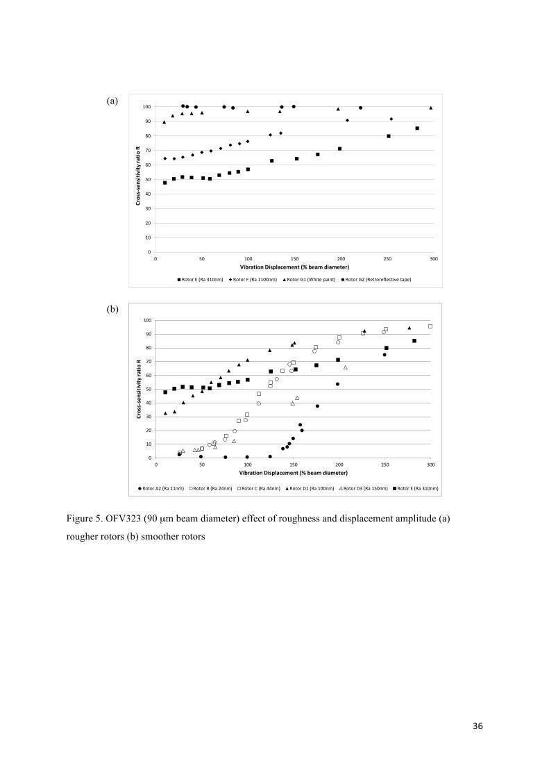
3.3 Cross-sensitivity: effect of vibration displacement

Further insight into these important trends is found by analysis of cross-sensitivity ratios as a function

of displacement (expressed as a percentage of beam diameter). Figure 5a shows the ratios calculated

for the measurements with the smaller beam instrument (OFV323) on the rougher and the treated

rotors. As expected, the cross-sensitivity ratio for a surface coated with retro-reflective tape is always

very close to 1 (mean 99.995%, standard deviation 0.425% across the full range). The lower mean

ratio for rotor G1 (coated with white paint) is driven by the lower values at lower displacements. This

trend of cross-sensitivity ratio increasing with vibration displacement is seen even more clearly in the

data for the measurements on rotor F (Ra 1100 nm), where the ratio takes values just above 60% at

low displacement, climbing to around 80% for a displacement equal to the beam diameter.

Measurements on rotor E (Ra 310 nm) exhibit even lower ratios but the same trend of increasing ratio

with increasing vibration displacement.

Figure 5b shows the other roughness extreme. Ratios close to zero are consistently found for the

group A rotors at vibration amplitudes close to or less than beam diameter. Ratios from this group all

follow the same trend and so, for clarity, only the ratios for rotor A2 (Ra 11 nm) are shown; the plot

illustrates how the low ratio is maintained up to 125% beam diameter. Data for other group A rotors

suggest a more cautious limit of 100% beam diameter is appropriate. It is for this reason that the ratios

summarised in Table 1 for the smaller beam instrument were based on vibration displacements close

to or less than 100% beam diameter. Thereafter, the ratios begin to increase markedly, eventually

reaching values close to 100% and matching the trend for the much rougher rotor E (Ra 310 nm) at a

vibration displacement of 250% beam diameter. Measurements on rotors B and C deliver trends that

12    

are indistinguishable from one another. At a vibration displacement of 25% beam diameter, the ratios

for these rotors and the group A rotors are very similar. In [29], where negligible cross-sensitivity was

found in a measurement on a rotor with roughness comparable to that of rotor B, vibration

displacement amplitudes were of the order of 1 µm, around 1% of the incident beam diameter, and so

that outcome is consistent with the findings of this current study. However, the ratio begins to rise for

the rotors B and C at much lower vibration displacements than seen in the group A rotor

measurements. The group D rotors (Ra from 100 to 150 nm) are represented by the data from D1 and

D3. The ratios for rotor D1 are not so dissimilar to those for rotor E (Ra 310 nm); certainly the

relatively high ratios at low displacements suggest that the polished-circular rotor model does not

apply. The rougher but rounder rotor, D3, however, almost follows the trend of the rotors B and C,

suggesting the opposite.

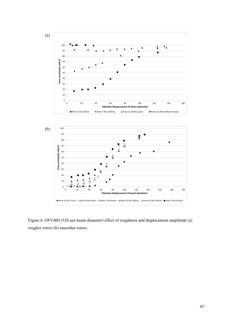
Figures 6a&b show the equivalent data for the larger (520 µm) beam instrument, OFV400. The cross-

sensitivity ratios for a surface coated with retro-reflective tape are again very close to 100% while

those for the painted surface are around 10% lower, as shown in Figure 6a. Compared to the results

from the smaller beam instrument, measurements on rotors E (Ra 310 nm) and F (Ra 1100nm) deliver

lower ratios but the variation with vibration displacement follows a similar trend. Ratios are also

generally lower for the more polished rotors, as shown in Figure 6b, but they still show the familiar

trend of increasing ratios with increasing vibration displacement. Measurements on the group A

rotors, again represented by rotor A2, have negligible cross-sensitivity up to approximately 40% beam

diameter. A compromise value of 50% was used for the data in table I to ensure sufficient data points

contributed to each calculation. Rotors B and C again exhibit near identical trends; here the maximum

acceptable vibration displacement is harder to ascertain but a figure of 10% is suggested. Smaller

displacements will be considered in a further study. Once more, measurements on rotor D3 (Ra 150

nm) exhibit very low ratios at low displacements while measurements on rotor D1 (Ra 100nm) exhibit

values around 10% at low displacements – much higher than those from rotor D3 and too high to be

considered negligible. For all of the more polished rotors, quite a similar trend is observed with a clear

increase in gradient at around 40% beam diameter.

Figures 5b and 6b throw light on the mechanism behind the observed increase in cross-sensitivity

ratio with vibration displacement for the polished rotors. Referring back to section 2.2, as vibration

displacement approaches beam diameter, the collected light intensity from the specular reflection

along the line passing through the rotor centre diminishes. The light collection becomes increasingly

dominated by diffuse scatter occurring because even the smoothest rotors tested here are not perfectly

smooth. Herein lies the connection between cross-sensitivity ratio and light collection; when diffuse

scatter (with which speckle patterns are associated) dominates, the ratio will be close to 100% but

when specular reflection dominates, the ratio will be close to zero. At intermediate values of

13    

roughness, there are significant diffuse and specular contributions which compete to make the

dominant contribution to collected light intensity, resulting in ratios with intermediate values.

Observation of the y-radial measurement on a group A rotor (with sinusoidal x-radial vibration only)

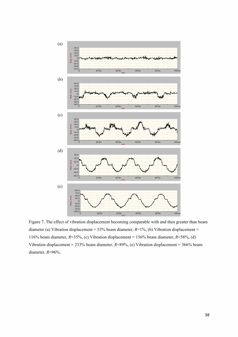
supports this explanation, as shown in Figure 7 for measurements at 5 vibration amplitudes from 53%

to 366% beam diameter. At the smallest vibration displacement, Figure 7a, there is negligible cross-

sensitivity but, as the amplitude grows, regions begin to appear in the plot where a part of a sinusoidal

motion becomes apparent. These regions correspond to those parts of the vibration cycle where the

light collection is dominated not by specular reflection but by diffuse scatter. As the vibration

amplitude increases, the proportion of the vibration cycle where this is the case also increases. In

Figure 7b, comparison with the x-radial measurement (not shown) indicates that the higher measured

velocities occur at the time that the rotor is at one of the extremes of its displacement cycle. In Figure

7c, these regions begin to appear in both halves of the vibration cycle, corresponding to both ends of

the rotor’s displacement cycle. At 233% beam diameter, Figure 7d shows this effect quite clearly

while in Figure 7e, with the largest measured vibration, only short regions remain apparent where no

oscillatory motion is observed. Comparison with the x-radial velocity shows that these regions

correspond to the times when the rotor passes through its mid-position such that the specular

reflection briefly dominates. Elsewhere the collected light is dominated by diffuse scatter and the

measured velocity takes the near-sinusoidal form. While these plots help to understand the mechanism

behind the increase in cross-sensitivity ratio with increasing vibration displacement, they also show

the considerable distortion of the genuine target velocity. This is not a route to high quality

measurements of high vibration displacements on polished-circular rotors.

3.4 Practical implications

The data presented in Figures 5-7 have profound, practical implications for radial vibration

measurements on rotors using LDV. When the cross-sensitivity ratio is close to zero, measurements

are straightforward but the circumstances necessary for this condition need careful definition. The

data for the instrument with a 90 µm beam suggest that the polished-circular rotor model applies to

measurements on rotors with Ra up to 10 nm for vibration displacement up to 100% beam diameter

and to rotors with Ra in the range 10 to 50 nm for vibration displacement up to 25% beam diameter.

For the instrument with 520 µm beam, the polished-circular rotor model appears to apply for

measurements on rotors with Ra up to 10 nm for vibration displacement up to 40% beam diameter and

to rotors with Ra from 10 to 50 nm for vibration displacement up to 10% beam diameter. Based on the

data from the group A and B rotors and rotor D3, rotor out-of-roundness should not exceed 10 µm in

such measurements but this requires further investigation that might lead to some relaxation of the

condition. Beam diameter has little effect on pseudo-vibration [33] so the instrument with the larger

beam diameter is the preferred option of the two considered here. Radial misalignment (the

14    

perpendicular separation between the centre-line of the laser beam and a parallel line passing through

the rotor centre) must also be much smaller than beam diameter which may be challenging in real

applications with smaller laser beams. Continuous checks for loss of signal (drop-out) must be made.

When the cross-sensitivity ratio is 100%, measurements can be made but post-processing, as will be

described in section 4, is essential to resolve individual vibration components. Measurements

presented here suggest that the necessary conditions are only properly met when surfaces are treated

with retro-reflective tape. Smaller beams are preferable because they offer lower pseudo-vibration

levels. When the cross-sensitivity ratio takes an intermediate value, measurements cannot be reliably

made because there is currently no means to estimate what value the ratio will take and this problem

is emphasised by the unpredictable behaviour of the group D rotors with roughness in the range Ra

100 to 150 nm. The user must either arrange for polished-circular surfaces from which to take

measurements or treat the surface with retro-reflective tape and post-process. The user has to be sure

of the cross-sensitivity ratio and so only the cases of R=0 and R=100% are worthy of further

consideration. This paper will now consider the measurement errors associated with these two

important cases.

4. Post-processing for radial vibration measurements with R=100%

In this section, the importance of post-processing for measurements with R=100% is demonstrated

quantitatively through simulation. Such data has not previously been reported. The post-processing

method [28] requires measurements of x- and y-radial velocity and totΩ . The post-processor consists

of a resolution algorithm complemented by a correction algorithm necessary when totΩ has a time-

varying component due to speed fluctuations (including torsional vibrations or roll). Both algorithms

are implemented in the frequency domain and function with negligible associated delay.

4.1 Constant rotation speed

The resolution algorithm is formulated in terms of the alternating components of measured velocities,

mxU~ and myU~ , and the mean value of rotation speed, totΩ , and is applied frequency-by-frequency as

follows:

( ) ( )n

dtUUFTWXt

mytotmxnnω

ωω ⎥⎦⎤

⎢⎣⎡ Ω−= ∫0

~~ (17a)

( ) ( )n

dtUUFTWYt

mxtotmynnω

ωω ⎥⎦⎤

⎢⎣⎡ Ω+= ∫0

~~ (17b)

15    

where ( )nW ω is a frequency dependent weighting factor given by:

( ) ( )222totnnnW Ω−= ωωω (17c)

Brief details of the implementation of the resolution algorithm are included in Appendix C. In the

simulation work presented here, the calculations are made in MATLAB code while a LabVIEW based

post-processor was used in earlier experimental work.

Simulating equal amplitude, harmonic x- and y-radial vibrations with 36 random values of phase

difference (in the range –π to π) emphasises the significance of this cross-sensitivity and the

importance of post-processing. Without misalignments or measurement noise, Figure 8 shows the

apparent error in the measured velocity as a percentage of genuine velocity for the x-measurement.

This apparent error is a function of phase and the figure shows the mean error together with maximum

and minimum errors across the rotation order range. The mean error varies between approximately

1000% at very low orders to just below 10% around 10th order. After resolution, mean errors are

effectively zero for amplitude and phase, as shown for the x-velocity in Figures 9a&b. These data are

independent of velocity amplitude and show quantitatively the significance of the cross-sensitivities

encountered in radial vibration measurements. They confirm that use of this algorithm to resolve

vibration velocities is absolutely essential. Data for y-radial vibration are identical and not shown for

the analysis in this section.

At first order, totn Ω=ω , the weighting function ( )nW ω is seen to be infinite and the bracketed

functions in equations (17a&b) evaluate to zero. The resolved velocity cannot be determined and all

resolved velocities including Figures 9a&b do not show data points at first order. This is a

fundamental limitation of the use of LDV for this application and not a consequence of the post-

processing method [26].

4.2 Speed fluctuations

Equations (17a&b) are only approximate when there is time dependence in totΩ , denoted totΔΩ . In

this case, the resolution algorithm outputs are no longer equal to just the resolved vibration velocities,

as in equations (17a&b), but include additional terms:

( )

( ) ( )n

n

dtxydtxyFTWX

dtUUFTW

t

tottottot

t

tottottotnn

t

mytotmxn

ω

ω

ωω

ω

⎥⎦⎤

⎢⎣⎡ ⎟

⎠⎞⎜

⎝⎛ ΔΩΩ+ΔΩ−⎟

⎠⎞⎜

⎝⎛ ΔΩΩ+ΔΩ+

=⎥⎦⎤

⎢⎣⎡ Ω−

∫∫

∫

0000

0

~~

(18a)

16    

( )

( ) ( )n

n

dtyxdtyxFTWY

dtUUFTW

t

tottottot

t

tottottotnn

t

mxtotmyn

ω

ω

ωω

ω

⎥⎦⎤

⎢⎣⎡ ⎟

⎠⎞⎜

⎝⎛ ΔΩΩ−ΔΩ−⎟

⎠⎞⎜

⎝⎛ ΔΩΩ−ΔΩ−

=⎥⎦⎤

⎢⎣⎡ Ω+

∫∫

∫

0000

0

~~

(18b)

The user must try to reduce the radial misalignments 0x and 0y to zero but it is difficult to achieve

this sufficiently; radial misalignments would need to be much less than vibration displacement

amplitudes to be negligible. The error associated with the combination of totΔΩ and the vibration

displacements, however, can be reduced. A correction algorithm has been developed from which

improved estimates of resolved velocity, 1+mX and 1+mY , are calculated based on the first estimate of

the resolved velocities (directly from the resolution algorithm), 1X and 1Y , and the mth estimate of

the resolved vibration displacements in the time domain (excluding the synchronous component), mx

and my :

( ) ( ) ( )n

dtxyFTWXXt

mtottotmtotnnnmω

ωωω ⎥⎦⎤

⎢⎣⎡ ΔΩΩ+ΔΩ−= ∫+ 011

(19a)

( ) ( ) ( )n

dtyxFTWYYt

mtottotmtotnnnmω

ωωω ⎥⎦⎤

⎢⎣⎡ ΔΩΩ−ΔΩ+= ∫+ 011

(19b)

Brief details of the implementation of the correction algorithm are included in Appendix C.

The effect of speed fluctuation on the resolved outputs is demonstrated in Figures 10a&b. Equal

amplitude, harmonic x- and y-radial vibrations with 16 random values of phase difference, combined

with 16 independent broadband speed variations (RMS level of 2% of rotation speed), are simulated.

Figure 10a shows that the RMS error in resolved amplitude is now up to 1% with a mean value for the

plotted points of 0.14%. The corresponding phase error is in the region of 1 to 10 mrad at lower

orders, falling to 0.1 mrad at higher orders. Error increases as the RMS broadband speed variation

increases but there is no dependency on radial vibration amplitude.

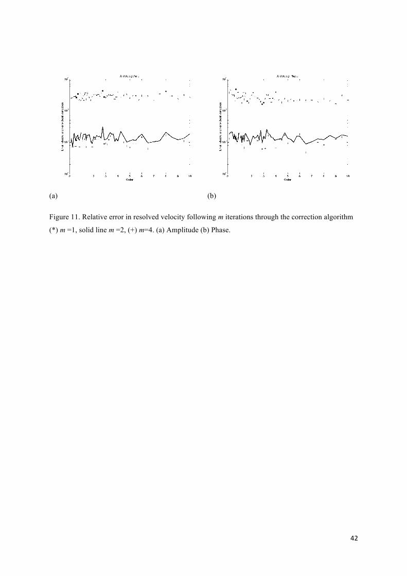
After a first iteration through the correction algorithm (m=1), Figures 11a&b show how the error

across the order range is reduced to around 3% of its uncorrected level for both amplitude and phase.

After a further iteration, these figures show that there is a further reduction to around 0.15% and, in an

absolute sense, errors are now very low at less than 0.003% for amplitude and 0.02 mrad for phase.

Further error reductions are found, to 0.1% of the uncorrected levels after 4 iterations but there is no

further improvement after 8 iterations. Routine addition of two iterations through the correction

17    

algorithm is, therefore, recommended as a good compromise between error reduction and post-

processing time.

5. Noise and misalignments in real measurements

In practice, of course, measurements are affected by noise and by small but inevitable radial and

angular misalignments. In this application, the principal source of noise is known as pseudo-vibration

[32). On surfaces with R=100%, this is the result of the laser speckle effect, while on polished

surfaces (R=0) it is a consequence of changes in the precise region of the illuminating beam from

which the dominant portion of the collected light originates. Such noise is periodic at rotation speed

with content up to high orders. In this section, the combined effects of measurement noise and

misalignments will be simulated to quantify the likely level of errors resulting from different

measurement scenarios.

5.1 Pseudo-vibration

Likely pseudo-vibration levels have been quantified [33], acknowledging the effects of incident beam

diameter and surface roughness as well as their instrument-specific nature. The following figures

represent the RMS level over a bandwidth of 10 orders. For rougher or treated surfaces (R=100%), a

level of 2 µm s-1/rad s-1 is typical for an incident beam diameter around 100 µm with a level of

5 µm s-1/rad s-1 typical for a 500 µm beam. For polished surfaces (R=0), 0.5 µm s-1/rad s-1 is a typical

level for both beams.

For a rough rotor and using an RMS pseudo-vibration level over 10 orders of 2 µm s-1/rad s-1, the

vibrometer outputs shown in Figures 12a&b have been simulated. Periodic speckle noise is clear,

together with random measurement noise at a relative level based on experimental observations (RMS

of one-twentieth of the RMS of periodic noise). This simulation has equal amplitude, second order

radial vibrations with amplitudes of 0.1 mm s-1/rad s-1. Normalisation by rotation speed is a

convenient approach to both simulation and to presentation of data and the chosen levels correspond

to 13 mm/s at 1200RPM or 31 mm/s at 3000RPM. These are realistic, medium severity levels.

5.2 Misalignments

The new modelling framework [31] readily accommodates misalignments into the prediction of

measured velocity. For an x-radial measurement, translational misalignments xy0 and xz0 identify the

chosen ‘known’ point in the yz plane:

[ ][ ]Txxx zyzyxr 000 0ˆˆˆ= (20a)

18    

Beam orientation is written as an initial alignment in the x-direction modified by angular

misalignments, xβ around the y-axis and xγ around the z-axis:

[ ][ ][ ][ ]Txxx yzzyxb 001,,ˆˆˆˆ βγ=− (20b)

For the y-radial measurement, translational misalignments yx0 and yz0 identify the chosen ‘known’

point in the xz plane and beam orientation is written as an initial alignment in the y-direction modified

by angular misalignments, yα around the x-axis and yγ around the z-axis. The equivalent expressions

are written:

[ ][ ]Tyyy zxzyxr 000 0ˆˆˆ= (21a)

[ ][ ][ ][ ]Tyyy xzzyxb 010,,ˆˆˆˆ αγ=− (21b)

Equations (20a&b) and (21a&b) can then be substituted into the measured velocity equations for the

rough and polished-circular rotor measurements. The vector formulations of equations (7) and (14),

rather than an expanded form like equation (B3), are best suited to simulation. Noise can be added

directly to each simulated measurement. Typical angular and translational misalignments and noise

are treated as inputs to the simulations. From this basis, an analysis can be made not just of the effects

of misalignments and measurement noise but also of the influence of motion components other than

the radial components themselves. For example, angular misalignments will result in sensitivity to

axial vibrations and axial misalignments will result in sensitivity to pitch and yaw vibrations.

For post-processing, measurements of the mean and the fluctuating components of the measured

rotation speed are required. Imperfections in these measurements can also be included in the

simulations; an error e has been included in the simulated mean speed measurement, tots ,Ω , and,

based on the likelihood of the use of a parallel beam laser vibrometer for measurement of the

fluctuating component, pseudo-vibration can be included via the quantity tots ,ΔΩ . The chosen forms

are:

( ) tottots e Ω+=Ω 1, (22a)

( ) Ω+Ω−Ω=ΔΩ ntottottots, (22b)

19    

An RMS pseudo-vibration level over 10 orders of 0.07 deg s-1/rad s-1 (based on beam diameter 520

µm, shaft diameter 15 mm, surface coated in retro-reflective tape [33]) is appropriate for the

simulations.

5.3 Simulations: sensitivity to radial vibrations only

The intention of this section is to present simulations that demonstrate the relative effect of each

source of error in rough and polished-circular rotor measurements. The error calculated at each

rotation order is a consequence of simultaneous x- and y-radial vibrations at that same order with

amplitudes of 0.1 mm s-1/rad s-1 , unless stated otherwise. In all cases, realistic values for

misalignments (see Appendix D) are used based on the authors’ experience but the reader must be

mindful that predicted errors are obviously very dependent on these chosen values. The paper has,

however, presented the full theoretical basis to these simulations, enabling another investigator to

model their specific scenarios and predict likely error levels.

Generally, only x-radial error spectra are presented as the corresponding y-radial data are identical. In

addition, the resolution in the plots is made finer in the more rapidly changing regions of the spectra

i.e. close to the synchronous frequency. Only ‘good’ setups contribute to the data presented; in real

measurements excessive DC velocity is indicative of radial misalignment and is routinely minimised.

From the authors’ experience, DC velocity can be reduced to levels corresponding to maximum radial

misalignments around 0.2 mm. Simulations include a check to exclude individual setups that would

be rejected in real measurements.

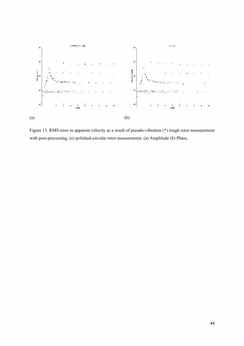
The effect of pseudo-vibration is shown in Figures 13a&b. In this simulation, 32 random values of

phase difference between the radial vibrations (in the range –π to π) are combined with 64

independent measurement noises (with RMS levels as set out in section 5.1) in the simulated radial

measurements, equating to a total of 2048 scenarios. For the rough rotor simulation, amplitude errors

of around 1% appear at the integer orders where periodic speckle noise occurs and 0.1% to 0.01%

elsewhere. Phase errors of around 10 mrad appear at the integer orders and 0.1 to 1 mrad elsewhere.

The polished-circular rotor simulation reflects the lower noise levels encountered while the advantage

of there being no need for resolution brings significant benefit around the synchronous frequency. In

both cases, errors change in inverse proportion to any change in vibration amplitudes i.e. a tenfold

increase in vibration amplitude results in a tenfold decrease in errors.

Figures 14a&b show the effect of typical misalignments. 21875 ‘good’ misaligned setups are

simulated (from initial consideration of 42875 setups) with 16 random values of phase difference

between the radial vibrations, producing 350000 scenarios. For the rough rotor simulation, amplitude

errors of around 0.2% appear at frequencies away from synchronous, rising to 2% close to

synchronous. Similarly, phase errors of around 2 mrad appear at frequencies away from synchronous,

20    

rising to 30 mrad close to synchronous. Comparable data for the polished-circular rotor show

expected error levels at 0.2% for amplitude and 5 mrad for phase. Vibration amplitude does not affect

these levels. With only x- and y-radial vibrations, angular misalignments around x- and y-axes (which

deliver sensitivity to z-vibration) have no significant effect and the same is true of translational

misalignments (which would deliver sensitivity to angular vibrations). Angular misalignment around

the z-axis is the critical parameter.

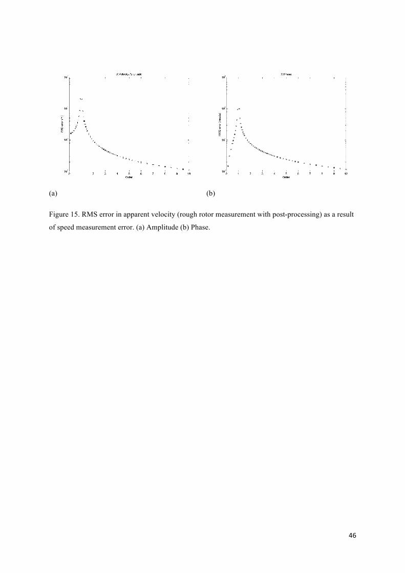
Speed measurement error is the subject of Figures 15a&b. Errors from -2.5% to 2.5%, in steps of

0.5% are considered in combination with 32 random values of phase difference between the radial

vibrations (a total of 352 scenarios). This error is unique to the rough rotor measurement; amplitude

error is close to 2% at low frequencies, rising to 20% near synchronous before falling to around 1% at

second order and 0.1% by tenth order while phase error rises from 1 mrad at very low frequency to

100 mrad near synchronous before falling to less than 10 mrad at second order and almost 1 mrad at

tenth order. There is no effect of vibration amplitude on this error.

In the presence of x- and y-radial vibrations only, these three sources of error are dominant. Figures

16a&b show their combination (16 independent measurement noises, 21875 misaligned setups, speed

errors from -2.5% to 2.5%, in steps of 1.25% and 16 phases between the radial vibrations resulting in

28 million scenarios). Speckle noise dominates the rough rotor measurement at integer orders from 2

upwards. Away from the integer orders, speed measurement error dominates up to around fifth order

after which misalignments become the significant effect. Errors associated with the speed variations

considered in Figures 10 and 11 are at least an order of magnitude lower than these levels and so are

negligible. Nonetheless, this simulation was repeated for the same set of 28 million scenarios but with

the addition of four iterations around the correction algorithm which confirmed that there are no

adverse effects on these error levels associated with its use. For the polished-circular rotor

measurement, misalignment is the critical source of error for both amplitude and phase, although

pseudo-vibration does make some additional contribution at integer orders.

The cross-sensitivity in the rough rotor measurement makes the ratio of radial amplitudes a potentially

important factor. All simulated data presented to this point have had equal amplitude radial vibrations.

For the same set of scenarios as used in Figures 16a&b, Figures 17a-d explore the effect of

differences between the radial vibration amplitudes. In all these plots, the ratio of x-radial to y-radial

amplitude is 10. The solid lines are for the case where the ratio of 10 is achieved by reducing the y-

amplitude by a factor of 10 while the dashed line is the result of increasing the x-amplitude by a factor

of 10. The ‘relative error’ plotted refers to the error for an amplitude ratio of 10 relative to that for an

amplitude ratio of 1.

21    

In each plot, the solid and dashed lines are almost identical. This means that it is the ratio that sets the

general trend rather than the absolute x- and y-radial amplitudes. Figure 17a shows that, for the larger

vibration component (in this case x-radial), the error in the resolved velocity is unchanged at very low

frequencies but then reduces significantly over the first few orders towards a value of 0.1. The relative

phase error shown in Figure 17b takes a value between 0.2 and 0.3 across the whole order range.

Unsurprisingly, the errors for the smaller radial component are increased, as shown in Figures 17c&d.

Amplitude error follows a reciprocal trend compared to the larger component while the phase error is

a factor of 10 higher across the whole order range.

These four figures also show the error values at integer orders which are driven by speckle noise and

are therefore dependent on absolute vibration amplitude. For the larger component, amplitude and

phase errors are largely unchanged (approximately 10% to 20% lower) when that same component’s

amplitude is unchanged from the equal amplitude simulations but they are reduced across the order

range by 80% to 90% when that component’s amplitude is increased by a factor of 10. For the smaller

component, a reduction in its amplitude by a factor of 10 results in error levels increased by a similar

factor. When its absolute amplitude is maintained, however, the errors in the resolved amplitude and

phase still grow significantly, by factors between 3 and 6.

5.4. Simulations: sensitivity to axial and angular vibrations

Inevitable misalignments will also result in sensitivities to other motion components and this section

explores sensitivity to axial and pitch or yaw vibrations as well as speed variation. In these

simulations, radial vibrations are absent and only the motion under consideration is present. In each

case, there are 140625 ‘good’ (but misaligned) setups (from 390625 considered) and there are no

effects of vibration amplitude on any of the sensitivities.

Figure 18 shows sensitivities to axial vibrations which occur principally as a result of angular

misalignments. A harmonic axial vibration is simulated at each order of interest to generate the

sensitivity for that order. For a polished-circular rotor, typical sensitivities are between 0.2% and

0.5%. The difference between the sensitivities for the x- and y-radial measurements is the result of

slightly higher values for angular misalignment around the y-axes compared to those around the x-

axes, reflecting practical experience of angular alignment around horizontal and vertical axes. In the

rough rotor simulation, sensitivities are comparable at low orders, rising towards 5% close to

synchronous frequency before falling to reach values comparable with those for the polished-circular

rotor after a few orders.

Sensitivity to speed variations (which would include torsional vibrations) occurs only in the rough

rotor measurements as a consequence of y-radial misalignments in the x-radial measurement and vice-

versa. In this simulation, broadband speed variation is used. In all, 32 independent broadband speed

22    

variations are considered for each good setup. Sensitivity in the region of 0.1 mm s-1/rad s-1 is

apparent, as shown in Figure 19, rising by a factor of 10 in the region close to synchronous frequency.

For context, the figure also shows the sensitivity in the radial measurement before processing,

demonstrating that the effect of the resolution algorithm on this error is beneficial below around order

0.5 but detrimental between 0.5 and 3, beyond which the error in the resolved data is very similar to

that in the raw data. Since this sensitivity is the result of misalignments (the final bracketed terms in

equations (18a&b)), the correction algorithm would have no effect on this error. The effect of

equivalent misalignments on a y-radial measurement is identical.

Figure 20 shows the sensitivities to a pitch vibration driven principally by axial misalignment. A

harmonic pitch vibration is simulated at each order of interest to generate the sensitivity at each order.

Looking first at the polished-circular rotor simulation, the greater sensitivity to pitch vibration appears

understandably in the y-radial measurement. Sensitivity in the x-radial measurement is much lower;

combination of axial misalignment and angular misalignment around the z-axis produce a very small

sensitivity to this motion. In the rough rotor data, the sensitivity in the y-radial measurement is

comparable with that encountered in the polished-circular rotor measurement except for a range

approximately half an order either side of the synchronous frequency where sensitivity is up to a

factor of 10 higher. The sensitivity in the x-radial measurement is much higher than for the equivalent

polished-circular rotor measurement; it is comparable with the y-radial rough rotor measurement

around the synchronous frequency but lower elsewhere. Sensitivity to a yaw vibration would follow

the same trends with the x and y plots reversed.

6. Conclusions

This paper has combined an experimental study of the cross-sensitivity encountered in LDV

measurements of rotor radial vibration with a quantitative evaluation of measurement errors, including

sensitivities to other motions, based on simulation. The evaluation of the effects of misalignments and

other motions, for both rough and polished-circular rotors, was made possible by a recently developed

framework for a comprehensive mathematical prediction of measured velocity that is without

approximation. The ease in modelling adds further weight to the assertion [31] that this modelling

framework can be applied universally for laser vibrometry applications.

The study of the effect on cross-sensitivity of surface roughness and treatment resolved a significant

inconsistency in the published literature and delivered an important conclusion regarding the rotor

surface conditions under which measurements can be made. Of the rotors tested in this study, those

with surface roughness up to 50 nm and out-of-roundness below 10 µm satisfied the polished-circular

rotor definition, provided vibration displacement does not exceed a specific threshold related to beam

23    

diameter. Only rotors coated in retro-reflective tape satisfied the rough rotor definition although the

painted surface was close. The extent of the cross sensitivity did not reach 100% for the roughest of

the rotors tested here (Ra 1100 nm) and so, when polished-circular surfaces are not available, rotor

surfaces must be treated with retro-reflective tape. In such circumstances, measurements can again be

made reliably (except at the synchronous frequency) but measurements must be post-processed to

resolve the individual radial motion components.

The overall conclusion to be drawn from the second part of the paper is that measurement errors and

sensitivities to other motions can be readily predicted for any specific measurement scenario. The

essential requirement for post-processing of the rough rotor measurement has been demonstrated

quantitatively, as has the effectiveness of the resolution algorithm. In the presence of speed

fluctuations, the value of a complementary correction algorithm has also been confirmed and two

iterations through the algorithm are now recommended wherever speed fluctuation (including

torsional vibration) is present.

For equal amplitude radial vibrations, data have been generated for typical misalignments,

measurement noise and speed measurement errors to provide typical error levels for the user to have

in mind. Typical sensitivities to axial vibration, speed variation (including torsional vibration and roll)

and bending vibrations are also quantified for both rotor surface conditions. This study of the effects

of surface roughness, instrument misalignments and measurement noise delivers an essential practical

guide for the vibrometer user.

Acknowledgement

The authors would like to acknowledge support from the Engineering and Physical Sciences Research

Council for supporting Mario Tirabassi.

24    

REFERENCES

[1] E. Downham and R. Woods, The Rationale of Monitoring Vibration on Rotating Machinery in Continuously Operating Process Plant. Trans. ASME J. of Engineering for Industry (1971) 71-Vibr-96.

[2] R.B. Randall, State of the art in monitoring rotating machinery - Part 1. Sound Vib. 38(3) (2004) 14-21.

[3] M. Gilstrap, Transducer selection for vibration monitoring of rotating machinery. Sound Vib. 18(2) (1984) 22-24.

[4] W.C. Laws and A. Muszynska, Periodic and continuous vibration monitoring for preventive / predictive maintenance of rotating machinery. Trans. ASME J. Engineering for Gas Turbines and Power 109 (1987) 159-167. (DOI 10.1115/1.3240019)

[5] M Serridge, Fault detection techniques for reliable condition monitoring. Sound Vib. 23(5) (1989) 18-22.

[6] M Angelo, Choosing accelerometers for machinery health monitoring. Sound Vib. 24(12) (1990) 20-24.

[7] R.M. Jones, A Guide to the interpretation of machinery vibration measurements - Part 1. Sound Vib. 28(5) (1994) 24-35.

[8] R.M. Jones, A Guide to the interpretation of machinery vibration measurements - Part 2. Sound Vib. 28(9) (1994) 12-20.

[9] T.I. El-Wardany, D. Gao and M.A. Elbestawi, Tool condition monitoring in drilling using vibration signature analysis. Int. J. Mach. Tools Manufact. 36(6) (1996) 687-711. (DOI 10.1016/0890-6955(95)00058-5)

[10] S. Edwards, A. W. Lees and M. I. Friswell, Fault Diagnosis of Rotating Machinery. Shock and Vib. Digest 30(1) (1998) 4-13.

[11] E.P. Carden and P. Fanning, Vibration Based Condition Monitoring A Review, Structural Health Monitoring. 3(4) (2004) 355-377. (DOI 10.1177/1475921704047500)

[12] J.S. Mitchell, From Vibration Measurements to Condition Based Maintenance. Sound Vib. 41(1) (2007) 2-15.

[13] D.J. Ewins, Control of vibration and resonance in aero engines and rotating machinery - An overview. Int. J. Pressure Vessels and Piping 87(9) (2010) 504-510. (DOI 10.1016/j.ijpvp.2010.07.001)

[14] H.M. Hashemian, State-of-the-Art Predictive Maintenance Techniques. IEEE Trans. Instrumentation and Measurement 60(1) (2011) 226-236. (DOI 10.1109/TIM.2010.2047662)

[15] Q.V. Davis and W.K. Kulczyk, Vibrations of turbine blades measured by means of a laser. Nature 222 (1969) 475-476. (DOI 10.1038/222475a0)

[16] A.J. Oberholster and P.S. Heyns, Eulerian laser Doppler vibrometry: Online blade damage identification on a multi-blade test rotor, Mech. Syst. Signal Process. 25(1) (2011) 344-359. (DOI 10.1016/j.ymssp.2010.03.007)

[17] D. Di Maio and D.J. Ewins, Applications of continuous tracking SLDV measurement methods to axially symmetric rotating structures using different excitation methods, Mech. Syst. Signal Process. 24(8) (2010) 3013-3036. (DOI 10.1016/j.ymssp.2010.06.012)

[18] B.J. Halkon and S.J. Rothberg, Automatic post-processing of laser vibrometry data for rotor vibration measurements, Proceedings of the Eighth International Conference on Vibrations in Rotating Machinery, Swansea, UK, 2004, IMechE Conference Proceedings, pp. 215-230.

[19] K.M. Lee and A.A. Polycarpou, Dynamic microwaviness measurements of super smooth disk media used in magnetic hard disk drives. Mech. Syst. Signal Process. 20(6) (2006) 1322-1337. (DOI 10.1016/j.ymssp.2005.11.010)

25    

[20] Q.A. Jiang, C. Bi and S. Lin, Accurate Runout Measurement for HDD Spinning Motors and Disks, J. Advanced Mechanical Design Systems and Manufacturing 4(1) (2010) 324-335. (DOI 10.1299/jamdsm.4.324)

[21] B.S. Prasad, M.M.M. Sarcar and B.S. Ben, Development of a system for monitoring tool condition using acousto-optic emission signal in face turning-an experimental approach. Int. J. Advanced Manufacturing Tech. 51(1-4) (2010) 57-67. (DOI 10.1007/s00170-010-2607-5)

[22] M.L. Jakobsen, D. Harvey, T.A. Carolan, J.S. Barton, J.D.C. Jones and R.L. Reuben, Optical probing of acoustic emission from a rotating tool holder with a Sagnac interferometer. Proc. IMechE Part B J. Engineering Manufacture 213(2) (1999) 171-181. (DOI 10.1243/0954405991517344)

[23] K. Tatar and P. Gren, Measurement of milling tool vibrations during cutting using laser vibrometry. Int. J. Machine Tools and Manufacture 48(3-4) (2008) 380-387. (DOI 10.1016/j.ijmachtools.2007.09.009)

[24] S. Yu-sheng, Measurement of transient characteristics of motor by laser Doppler velocimetry. Chinese Physics 4(4) (1984) 903-906.

[25] T. Eiju and K. Matsuda, Determination of the central position of rotation of a rotating object by laser Doppler velocimetry. Opt. Eng. 30(11) (1991) 1825-1830. (DOI 10.1117/12.55982)

[26] S.J. Rothberg and N.A. Halliwell, Vibration measurements on rotating machinery using laser Doppler velocimetry. Trans. ASME J. Vib. Acoust. 116 (1994) 326-331. (DOI 10.1115/1.2930432)

[27] J.R. Bell and S.J. Rothberg, Laser vibrometers and contacting transducers, target rotation and six degree-of-freedom vibration: what do we really measure? J. Sound Vib. 237(2) (2000) 245-261. (DOI 10.1006/jsvi.2000.3053)

[28] B.J. Halkon and S.J. Rothberg, Rotor vibration measurements using laser Doppler vibrometry; essential post-processing for resolution of radial and pitch / yaw vibrations. Trans. ASME J. Vib. Acoust. 128 (2006) 8-20. (DOI 10.1115/1.2149389)

[29] K. Tatar, M. Rantatalo and P. Gren, Laser vibrometry measurements of an optically smooth rotating spindle. Mech. Syst. Signal Process. 21(4) (2007) 1739-1745. (DOI 10.1016/j.ymssp.2006.08.006)

[30] S.J. Rothberg, Radial Vibration Measurements Directly from Rotors using Laser Vibrometry: Uncertainty due to Surface Roughness, Proc. IMAC-XXV: A Conference and Exposition on Structural Dynamics, Orlando, Florida, USA, 2007, SEM Conference Proceedings, Paper #371.

[31] S.J. Rothberg and M. Tirabassi, A universal framework for modelling measured velocity in laser vibrometry with applications. Mech. Syst. Signal Process. 26 (2012) 141-166. (DOI 10.1016/j.ymssp.2011.06.022)

[32] P. Martin and S.J. Rothberg, Methods for the quantification of pseudo-vibration sensitivities in laser vibrometry. Meas. Sci. Technol. 22 (2011) 035302. (DOI 10.1088/0957-0233/22/3/035302)

[33] P. Martin and S.J. Rothberg, Pseudo-vibration sensitivities for commercial laser vibrometers. Mech. Syst. Signal Process. 25 (2011) 2753-2765. (DOI 10.1016/j.ymssp.2011.02.009)

[34] B.M. Watrasiewicz and M.J. Rudd, Laser Doppler measurement. Butterworths, London, 1976.

26    

Appendix A: Rotation Matrices

In the vector approach presented in this paper, rotation matrices are a convenient means to introduce

important features such as laser beam orientation and misalignment, and variations in the direction of

the shaft rotation axis. The matrices are dependent on the axis around which the rotation is performed.

For rotations α , β and γ around, respectively, the x-, y- and z-axes, the appropriate rotation

matrices are as follows [31):

[ ]⎥⎥⎥

⎦

⎤

⎢⎢⎢

⎣

⎡

−=

αα

ααα

cossin0sincos0001

,x (A.1a)

[ ]⎥⎥⎥

⎦

⎤

⎢⎢⎢

⎣

⎡

−

=

ββ

ββ

β

cos0sin010sin0cos

,y (A.1b)

[ ]⎥⎥⎥

⎦

⎤

⎢⎢⎢

⎣

⎡ −

=

1000cossin0sincos

, γγ

γγ

γz (A.1c)

The matrices can be applied singly or in series. Where rotations around more than one axis are by

large angles (e.g. for laser beam orientation), their order must be maintained. When rotations are by

small angles (e.g. for angular vibrations and misalignments), this is not necessary.

Appendix B: Vibration sets

The vector expressions in equation (7) for the target translational vibration velocity, [ ]Tzyx , and

displacement, [ ]Tzyx , are written as:

[ ][ ]TO zyxzyxV ˆˆˆ* = (B.1a)

[ ][ ]TzyxzyxOO ˆˆˆ* = (B.1b)

Using small angle approximations in equation (8c), equation (8a) expands as follows

[ ][ ]Tzxyyxzyx Ω+Ω−Ω+= θθθθθω ˆˆˆ (B.2)

27    

Combination of equations (3), (5b), (B.1a&b) and (B.2) then allows expansion of equation (7) as

follows:

( ) ( )[ ]( ) ( )[ ]

( ) ( )[ ]( )[ ]( )[ ]( )[ ]Ω+−+

Ω−++

Ω++−

Ω+−Ω−+−

Ω++Ω+−+

Ω−−Ω++=

z

xy

yx

yxxy

yxz

xyzm

yx

zx

zy

yxz

zxy

zyxU

θβγβγ

θθβγβ

θθβγβ

θθθθβ

θθθβγ

θθθβγ

coscoscossin

coscossin

cossinsin

sin

cossin

coscos

00

00

00

(B.3)

A full description of the terms in equation (B.3) has been presented [27]. Note that the measured

velocity is the sum of six terms, each the product of a combination of geometric parameters and a so-

called ‘vibration set’. These sets are an inseparable combination of motion parameters (shown in

square brackets) and are referred to by the parameter that is regarded as the intended measurement

and shown first in the sets. Section 2.1 makes specific use of the first two of these sets, the x-radial

and the y-radial sets. The reader should note the different angle convention used here compared to

[27].

Appendix C: Implementation of resolution and correction algorithms

The resolution algorithm as captured by equations (17a&b) is implemented in terms of the real (ℜ )

and imaginary (ℑ ) parts of the Fourier transform as follows [28]:

( ) ( ) [ ] [ ] [ ] [ ] ⎟⎟⎠

⎞⎜⎜⎝

⎛⎟⎟⎠

⎞⎜⎜⎝

⎛ℜ

Ω+ℑ+⎟⎟

⎠

⎞⎜⎜⎝

⎛ℑ

Ω−ℜ=

nnnn myn

totmxmy

n

totmxnn UUjUUWX

ωωωω ωωωω

~~~~ (C.1a)

( ) ( ) [ ] [ ] [ ] [ ] ⎟⎟⎠

⎞⎜⎜⎝

⎛⎟⎟⎠

⎞⎜⎜⎝

⎛ℜ

Ω−ℑ+⎟⎟

⎠

⎞⎜⎜⎝

⎛ℑ

Ω+ℜ=

nnnnmx

n

totmymx

n

totmynn UUjUUWY ωωωω ωω

ωω~~~~ (C.1b)

The correction algorithm as described by equations (19a&b) is implemented in similar fashion:

( ) ( )

( ) [ ] [ ] [ ] [ ]n

nnnn mtotn

totmtotmtot

n

totmtotn

nnm

xyjxyW

XX

ω

ωωωω ωωω

ωω

⎥⎦

⎤⎢⎣

⎡⎟⎟⎠

⎞⎜⎜⎝

⎛ΔΩℜ

Ω−ΔΩℑ+⎟⎟

⎠

⎞⎜⎜⎝

⎛ΔΩℑ

Ω+ΔΩℜ

−=+ 11

(C.2a)

28    

( ) ( )

( ) [ ] [ ] [ ] [ ]n

nnnn mtotn

totmtotmtot

n

totmtotn

nnm

yxjyxW

YY

ω

ωωωω ωωω

ωω

⎥⎦

⎤⎢⎣

⎡⎟⎟⎠

⎞⎜⎜⎝

⎛ΔΩℜ

Ω+ΔΩℑ+⎟⎟

⎠

⎞⎜⎜⎝

⎛ΔΩℑ

Ω−ΔΩℜ

+=+ 11

(C.2b)

where the mth estimates of the x- and y-radial vibration displacements in the time domain, mx and

my , are found from:

[ ] ( )[ ] ( )[ ]( )∑=

−−⎥⎦

⎤⎢⎣

⎡ℜ−ℑ==

N

nnmnm

nmm XjXFTXFTx

1

11 1ωω

ω (C.3a)

[ ] ( )[ ] ( )[ ]( )∑=

−−⎥⎦

⎤⎢⎣

⎡ℜ−ℑ==

N

nnmnm

nmm YjYFTYFTy

1

11 1ωω

ω (C.3b)

Appendix D: Misalignment values used in simulations

For all simulations except where stated otherwise:

yx0 and xy0 take values from -0.3 mm to 0.3 mm in steps of 0.1 mm

xz0 and yz0 are zero (section 5.3) or take values from -1 mm to 1 mm in steps of 0.5 mm (section

5.4)

xγ and yγ take values from -0.2O to 0.2O in steps of 0.1O

xβ takes values from -0.45O to 0.45O in steps of 0.15O (section 5.3)

xβ takes values from -0.5O to 0.5O in steps of 0.25O (section 5.4)

yα takes values from -0.2O to 0.2O in step of 0.1O

29    

Figure captions

Figure 1. Laser beam orientation.

Figure 2a. Laser beam orientation showing incident points on the displaced rotor.

Figure 2b. Laser beam orientation showing points used in vector polygons.

Figure 3. Reflection of light from a polished-circular rotor.

Figure 4. Cross-sensitivity experiments (a) experimental rig (b) laser beam alignment relative to rotor.

Figure 5. OFV323 (90 µm beam diameter) effect of roughness and displacement amplitude (a)

rougher rotors (b) smoother rotors

Figure 6. OFV400 (520 µm beam diameter) effect of roughness and displacement amplitude (a)

rougher rotors (b) smoother rotors.

Figure 7. The effect of vibration displacement becoming comparable with and then greater than beam

diameter (a) Vibration displacement = 53% beam diameter, R=1%, (b) Vibration displacement =

116% beam diameter, R=35%, (c) Vibration displacement = 156% beam diameter, R=58%, (d)

Vibration displacement = 233% beam diameter, R=89%, (e) Vibration displacement = 366% beam

diameter, R=96%.

Figure 8. Mean (solid line) and maximum / minimum (dashed lines) RMS error in the measured

velocity due to cross-sensitivity, expressed as a percentage of genuine velocity.

Figure 9. RMS error for x-radial velocity after post-processing (a) Amplitude (b) Phase.

Figure 10. RMS error in resolved velocity as a result of broadband speed variation (a) Amplitude (b)

Phase.

Figure 11. Relative error in resolved velocity following m iterations through the correction algorithm

(*) m =1, solid line m =2, (+) m=4. (a) Amplitude (b) Phase.

Figure 12. Simulated laser vibrometer outputs showing pseudo-vibration (RMS over 10 orders of

2 µm s-1/rad s-1, and equal amplitude, second order radial vibrations with amplitudes of

0.1 mm s-1/ rad s-1 . (a) x-radial measurement (b) y-radial measurement.

Figure 13. RMS error in apparent velocity as a result of pseudo-vibration (*) rough rotor measurement

with post-processing, (o) polished-circular rotor measurement. (a) Amplitude (b) Phase.

30    

Figure 14. RMS error in apparent velocity as a result of misalignments (*) rough rotor measurement

with post-processing, (o) polished-circular rotor measurement.( a) Amplitude (b) Phase.

Figure 15. RMS error in apparent velocity (rough rotor measurement with post-processing) as a result

of speed measurement error. (a) Amplitude (b) Phase.

Figure 16. RMS error in apparent velocity as a result of the combination of pseudo-vibration,

misalignments and speed measurement error (*) rough rotor measurement with post-processing, (o)

polished-circular rotor measurement. (a) Amplitude (b) Phase.

Figure 17. For rough rotor measurement with post-processing, relative error in apparent velocity with ratio of 10 between x- and y- radial vibration amplitudes. Solid line and * markers: y-radial amplitude reduced by factor of 10 relative to Figure 16 simulation. Dashed line and + markers: x-radial amplitude increased by factor of 10 relative to Figure 16 simulation. (a) x-radial amplitude (b) x-radial phase (c) y-radial amplitude (d) y-radial phase.

Figure 18. Axial velocity sensitivity due to misalignments. (*) resolved x-radial velocity in rough

rotor measurement with post-processing, (+) resolved y-radial velocity in rough rotor measurement

with post-processing, solid line - x-radial velocity in polished-circular rotor measurement, dashed line

- y-radial velocity in polished-circular rotor measurement.

Figure 19. Speed variation sensitivity in x-radial velocity due to misalignments in rough rotor

measurement. (*) with post-processing, solid line without post-processing

Figure 20. Pitch sensitivity due to misalignments. (*) resolved x-radial velocity in rough rotor

measurement with post-processing, (+) resolved y-radial velocity in rough rotor measurement with

post-processing, solid line - x-radial velocity in polished-circular rotor measurement, dashed line - y-

radial velocity in polished-circular rotor measurement.

Table captions

Table 1. Roughness and roundness of rotor samples and cross-sensitivity ratios for OFV323 (vibration

displacement close to or less than beam diameter) and OFV400 (vibration displacement close to or

less than 0.5 x beam diameter).

31    

Table 1. Roughness and roundness of rotor samples and cross-sensitivity ratios for OFV323 (vibration

displacement close to or less than beam diameter) and OFV400 (vibration displacement close to or

less than 0.5 x beam diameter).

Rotor ID Roughness Ra (nm) Out-of-roundness (µm)

cross sensitivity ratio (%) mean (standard deviation)

OFV323, 90 µm beam

OFV400, 520 µm beam

A1 9.7 6.0 0.90 (0.45) 3.0 (0.82) A2 11 6.7 1.3 (0.84) 1.2 (0.75) A3 12 5.8 1.5 (1.0) 1.2 (0.59) B 24 4.5 13 (8.2) 8.4 (4.1) C 44 6.5 16 (11) 6.4 (3.2) D1 100 23 52 (14) 14 (4.1) D2 130 36 47 (11) 2.0 (2.5) D3 150 12 7.5 (2.8) 1.3 (0.70) E 310 1.0 52 (2.7) 22 (4.7) F 1100 4.7 70 (4.3) 59 (7.3) G1 White paint n/a 95 (2.6) 91 (1.2) G2 Retro-reflective tape n/a 100 (1.6) 100 (1.4)

32    

x

y

z

γinb−

βsin

γβ coscos

γβ sincos

β

 

Figure 1. Laser beam orientation.

33    

O

O*Q

P

z

y

x

P’

Displaced rotor position

Original rotor position

Original point of incidence

 

Figure 2a. Laser beam orientation showing incident points on the displaced rotor.

O*

Q

O

P

0rz

y

x

Rotationaxis

p(t)

inbRz q(t) P’

0rΔ

p'(t)R

 

Figure 2b. Laser beam orientation showing points used in vector polygons.

34    

Emitting / collecting aperture

0 1

Reflected intensity profile

Polished-circular rotor

 

Figure 3. Reflection of light from a polished-circular rotor.

35    

x

y

z

x-radial measurement

y-radial measurement

Direction of oscillation

(a) (b)  

Figure 4. Cross-sensitivity experiments (a) experimental rig (b) laser beam alignment relative to rotor.

36    

(a)

0

10

20

30

40

50

60

70

80

90

100

0 50 100 150 200 250 300

Cross-­‐sensitivity  ra

tio  R

Vibration  Displacement  (%  beam  diameter)

Rotor  E  (Ra  310nm) Rotor  F  (Ra  1100nm) Rotor  G1  (White  paint) Rotor  G2  (Retroreflective  tape)

(b)

0

10

20

30

40

50

60

70

80

90

100

0 50 100 150 200 250 300

Cross-­‐sensitivity  ra

tio  R

Vibration  Displacement  (%  beam  diameter)

Rotor  A2  (Ra  11nm) Rotor  B  (Ra  24nm) Rotor  C  (Ra  44nm) Rotor  D1  (Ra  100nm) Rotor  D3  (Ra  150nm) Rotor  E  (Ra  310nm)

Figure 5. OFV323 (90 µm beam diameter) effect of roughness and displacement amplitude (a)

rougher rotors (b) smoother rotors

37    

(a)

0

10

20

30

40

50

60

70

80

90

100

0 20 40 60 80 100 120 140 160

Cross-­‐sesnitivity  ra

tio  R

Vibration  Displacement  (%  beam  diameter)

Rotor  E  (Ra  310nm) Rotor  F  (Ra  1100nm) Rotor  G1  (White  paint) Rotor  G2  (Retroreflective  tape)

(b)

0

10

20

30

40

50

60

70

80

90

100

0 20 40 60 80 100 120 140 160 180 200

Cross-­‐sensitivity  ra

tio  R

Vibration  Displacement  (%  beam  diameter)

Rotor  A2  (Ra  11nm) Rotor  B  (Ra  24nm) Rotor  C  (Ra  44nm) Rotor  D1  (Ra  100nm) Rotor  D3  (Ra  150nm) Rotor  E  (Ra  310nm)

 

Figure 6. OFV400 (520 µm beam diameter) effect of roughness and displacement amplitude (a)

rougher rotors (b) smoother rotors.

38    

(a)

(b)

(c)

0 20.0m 40.0m 60.0m 80.0m 100.0m-40.0-30.0-20.0-10.0

010.020.030.040.0

sec

Rea

l, m

m/s

(d)

0 20.0m 40.0m 60.0m 80.0m 100.0m-60.0

-40.0

-20.0

0

20.0

40.0

60.0

sec

Rea

l, m

m/s

(e)

0 20.0m 40.0m 60.0m 80.0m 100.0m-100.0

-75.0-50.0-25.0

025.050.075.0

100.0

sec

Rea

l, m

m/s

Figure 7. The effect of vibration displacement becoming comparable with and then greater than beam

diameter (a) Vibration displacement = 53% beam diameter, R=1%, (b) Vibration displacement =

116% beam diameter, R=35%, (c) Vibration displacement = 156% beam diameter, R=58%, (d)

Vibration displacement = 233% beam diameter, R=89%, (e) Vibration displacement = 366% beam

diameter, R=96%.

0 20.0m 40.0m 60.0m 80.0m 100.0m-40.0-30.0-20.0-10.0

010.020.030.040.0

secR

eal,

mm

/s

0 20.0m 40.0m 60.0m 80.0m 100.0m-40.0-30.0-20.0-10.0

010.020.030.040.0

sec

Rea

l, m

m/s

39    

Figure 8. Mean (solid line) and maximum / minimum (dashed lines) RMS error in the measured

velocity due to cross-sensitivity, expressed as a percentage of genuine velocity.

40    

(a) (b)

Figure 9. RMS error for x-radial velocity after post-processing (a) Amplitude (b) Phase.

41    

(a) (b)

Figure 10. RMS error in resolved velocity as a result of broadband speed variation (a) Amplitude (b)

Phase.

42    

(a) (b)

Figure 11. Relative error in resolved velocity following m iterations through the correction algorithm

(*) m =1, solid line m =2, (+) m=4. (a) Amplitude (b) Phase.

43    

(a) (b)

Figure 12. Simulated laser vibrometer outputs showing pseudo-vibration (RMS over 10 orders of

2 µm s-1/rad s-1, and equal amplitude, second order radial vibrations with amplitudes of

0.1 mm s-1/ rad s-1 . (a) x-radial measurement (b) y-radial measurement.

44    

(a) (b)

Figure 13. RMS error in apparent velocity as a result of pseudo-vibration (*) rough rotor measurement

with post-processing, (o) polished-circular rotor measurement. (a) Amplitude (b) Phase.

45    

(a) (b)

Figure 14. RMS error in apparent velocity as a result of misalignments (*) rough rotor measurement

with post-processing, (o) polished-circular rotor measurement.( a) Amplitude (b) Phase.

46    

(a) (b)

Figure 15. RMS error in apparent velocity (rough rotor measurement with post-processing) as a result

of speed measurement error. (a) Amplitude (b) Phase.

47    

(a) (b)

Figure 16. RMS error in apparent velocity as a result of the combination of pseudo-vibration,

misalignments and speed measurement error (*) rough rotor measurement with post-processing, (o)

polished-circular rotor measurement. (a) Amplitude (b) Phase.

48    

(a) (b)

(c) (d)

Figure 17. For rough rotor measurement with post-processing, relative error in apparent velocity with ratio of 10 between x- and y- radial vibration amplitudes. Solid line and * markers: y-radial amplitude reduced by factor of 10 relative to figure 16 simulation. Dashed line and + markers: x-radial amplitude increased by factor of 10 relative to figure 16 simulation. (a) x-radial amplitude (b) x-radial phase (c) y-radial amplitude (d) y-radial phase.

49    

Figure 18. Axial velocity sensitivity due to misalignments. (*) resolved x-radial velocity in rough

rotor measurement with post-processing, (+) resolved y-radial velocity in rough rotor measurement

with post-processing, solid line - x-radial velocity in polished-circular rotor measurement, dashed line

- y-radial velocity in polished-circular rotor measurement.

50    

Figure 19. Speed variation sensitivity in x-radial velocity due to misalignments in rough rotor

measurement. (*) with post-processing, solid line without post-processing

51    

Figure 20. Pitch sensitivity due to misalignments. (*) resolved x-radial velocity in rough rotor

measurement with post-processing, (+) resolved y-radial velocity in rough rotor measurement with

post-processing, solid line - x-radial velocity in polished-circular rotor measurement, dashed line - y-

radial velocity in polished-circular rotor measurement.