Radio Mathematics 1

Radio Mathematics

This supplement is a collection of tutorial information on a variety of mathematics used in Amateur Radio. Many of the fundamental relationships in electronics and radio are best expressed in the language of math. This chapter will expand in subsequent editions as it becomes clearer what information will be useful to readers. Material in this chapter has been collected from many sources, authors, and instructors over the years — the ARRL appreciates their contributions.

1 The Metric System

1.1 Metric Prefixes —the Language of RadioThe units of measurement employed in radio use the metric system

of prefixes. The metric system is used because the numbers involved cover such a wide range of values. Table 1 shows metric prefixes, symbols, and their meaning. The prefixes expand or shrink the units, multiplying them by the factor shown in the table. For example, a kilo-meter (km) is one thousand meters and a milli-meter (mm) is one-thousandth of a meter.

The most common prefixes you’ll encounter in radio are pico (p), nano (n), micro (µ), milli (m), centi (c), kilo (k), mega (M) and giga (G). It is important to use the proper case for the prefix letter. For example, M means one million and m means one-thousandth. Using the wrong case would make a big difference!

The metric system uses a basic unit for each different type of measurement. For example, the basic unit of length is the meter (or metre). The basic unit of volume is the liter (or litre). The unit for mass (or quantity of matter) is the gram. The new-ton is the metric unit of force, or weight, but we often use the gram to indicate how “heavy” something is by assuming a standard value of gravity.

Table 1 summarizes the most-used metric prefixes. The met-ric system expresses larger or smaller quantities by multiplying or dividing the basic unit by factors of 10 (10, 100, 1000, 10,000 and so on). These multiples result in a standard set of prefixes, which can be used with all the basic units. Even if you come across some terms you are unfamiliar with, you will be able to recognize the prefixes.

We can write these prefixes as powers of 10, as shown in Table 1. The power of 10 (called the exponent) shows how many times you must multiply (or divide) the basic unit by 10. For example, we can see from the table that kilo means 103. Let’s use the meter as an example. If you multiply a meter by 10 three times, you will have a kilometer. (1 m ×103 = 1 meter ×10×10 ×10 = 1000 meters, or 1 kilometer.)

If you multiply 1 meter by 10 six times, you have a megameter. (1 meter ×106 = 1 m ×10 ×10 ×10 ×10×10 ×10 = 1,000,000 meters or 1 megameter.)

Notice that the exponent for some of the prefixes is a negative number. This indicates that you must divide the basic unit by 10 that number of times. If you divide a meter by 10, you will have a decimeter. (1 meter ×10–1 = 1 m ÷ 10 = 0.1 meter, or 1 decime-ter.) When we write 10–6, it means you must divide by 10 six

2 Radio Mathematics

times. (1 meter ×10–6 = 1 m ÷ 10 ÷ 10 ÷ 10 ÷ 10 ÷ 10 ÷ 10 = 0.000001 meter, or 1 micrometer.)

We can easily write very large or very small numbers with this system. We can use the metric prefixes with the basic units, or we can use powers of 10. Many of the quantities used in basic elec-tronics are either very large or very small numbers, so we use these prefixes quite a bit. You should be sure you are familiar at least with the following prefixes and their associated powers of 10: giga (109), mega (106), kilo (103), centi (10–2), milli (10–3), micro (10–6) and pico (10–12).

Let’s try an example. For this example, we’ll use a term that you will run into quite often in the Handbook: hertz (abbreviated Hz, a unit that refers to the frequency of a radio wave). We have a receiver dial calibrated in kilohertz (kHz), and it shows a signal at a frequency of 28,450 kHz. Where would a dial calibrated in hertz show the signal? From Table 1 we see that kilo means times 1000. The basic unit of frequency is the hertz. That means that our signal is at 28,450 kHz ×1,000 = 28,450,000 hertz. There are 1000 hertz in 1 kilohertz, so 28,450,000 divided by 1000 gives us 28,450 kHz.

If we have a current of 3000 milliamperes, how many amperes is this? From Table 1 we see that milli means multiply by 0.001 or divide by 1000. Dividing 3000 milliamperes by 1000 gives us 3 amperes. The metric prefixes make it easy to use numbers that are a convenient size simply by changing the units. It is certainly easier to work with a measurement given as 3 amperes than as 3000 milliamperes!

Notice that it doesn’t matter what the units are or what they represent. Meters, hertz, amperes, volts, farads or watts make no

Table 1International System of Units (SI) — Metric Units

Prefix Symbol Multiplication FactorTera T 1012 = 1,000,000,000,000Giga G 109 = 1,000,000,000Mega M 106 = 1,000,000Kilo k 103 = 1000Hecto h 102 = 100Deca da 101 = 10Deci d 10-1 = 0.1Centi c 10-2 = 0.01Milli m 10-3 = 0.001Micro µ 10-6 = 0.000001Nano n 10-9 = 0.000000001Pico p 10-12 = 0.000000000001

1 M = 1000 k; 1 m=1000 µ = 1,000,000 n; 1 µ=1000 n=1,000,000 p

difference in how we use the prefixes. Each prefix represents a certain multiplication factor, and that value never changes.

1.2 Converting Between Types of UnitsConverting between different types of units requires a conversion

factor. The conversion factor is a value representing how many units of Type A are equivalent to a single unit of Type B, generally given as (amount of units of Type B) per (unit of Type A).

For example, the conversion factors between pounds (Type A) and kilograms (Type B) are 0.455 kg/lb and 2.2 lb/kg.

To decide which to use in converting units of Type A to Type B, select the factor with the Type B units in the numerator of the conver-sion factor. Multiply the amount of Type A units by the conversion factor.

For example, to convert 3 lb (Type A) to kg (Type B):1. Select the conversion factor with Type B units (kg) in the numer-

ator, 0.455 kg/lb2. Multiply the amount of Type A units by the conversion factor: 3 lb × 0.455 lb/kg = 1.37 kgSimilarly, to convert 3 kg (Type A) to lb (Type B):1. Select the conversion factor with Type B units (lb) in the numer-

ator, 2.2 lb/kg2. Multiply 3 kg × 2.2 lb/kg = 6.6 lbNote that these conversion factors are reciprocals. You can change

one conversion factor into the other by calculating 1 divided by the conversion factor. Exchange the numerator and denominator at the same time:

1/ (0.455 kg/lb) = 2.2 lb/kg and 1/ (2.2 lb/kg) = 0.455 kg/lb

You can also convert Type B units into Type A by dividing the amount of Type B units by the conversion factor from Type A to Type B:

10 kg / 0.455 kg/lb = 22 lb

Note that not all conversions are simple multiplications or divi-sions. Additional offsets or factors may be required. For example, to convert degrees Fahrenheit to degrees Celsius, the formula is:

Deg C = 5/9 × (Deg F – 32)

The Handbook’s Component Data and References chapter includes a table of conversion factors for US Customary Units and between US Customary Units and Metric Units. Online calculators abound. Google (www.google.com) provides a unit converter acces-sible by entering “convert [abbreviation or name for Type A units] to [abbreviation or name for Type B units]” into an Internet search window.

Radio Mathematics 3

2 Numbers and Notation2.1 Accuracy, Resolution, and Precision

The terms accuracy, precision, and resolution are often confused and used interchangeably, when they have very different meanings. When dealing with measurements and test instruments, it’s important to keep them straight.

• Accuracy is the ability of an instrument to make a measurement that reflects the actual value of the parameter being measured. An instrument’s accuracy is usually specified in percent or decibels (see below) referenced to some known standard.

• Precision refers to the smallest division of measurement that an instrument can make repeatedly. For example, a metric ruler divided into mm is more precise than one divided into cm.

• Resolution is the ability of an instrument to distinguish between two different quantities. If the smallest difference a meter can distin-guish between two currents is 0.1 mA, that is the meter’s resolution.

It is important to note that the three qualities are not necessarily mutually guaranteed. That is, a precise meter may not be accurate, or the resolution of an accurate meter may not be very high, or the precision of a meter may be greater than its resolution. It is important to understand the difference between the three.

2.2 Accuracy and Significant FiguresThe calculations you will find throughout the Handbook follow

the rules for accuracy of calculations. Accuracy is represented by the number of significant digits in a number. That is, the number of digits that carry numeric value information beyond order of magni-tude. For example, the numbers 0.123, 1.23, 12.3, 123, and 1,230 all have three significant digits.

The result of a calculation can only be as accurate as its least accu-rate measurement or known value. This is important because it is rare for measurements to be more accurate than a few percent. This limits the number of useful significant digits to two or three. Here’s another example; what is the current through a 12-Ω resistor if 4.6 V is applied? Ohm’s Law says I in amperes = 4.6 / 12 = 0.3833333... but because our most accurate numeric information only has two significant digits (12 and 4.6), strictly applying the significant digits calculation rule limits our answer to 0.38. One extra digit is often included, 0.383 in this case, to act as a guide in rounding off the answer.

Quite often this occurs because a calculator is used, and the result of a calculation fills the numeric window. Just because the calculator shows 9 digits after the decimal point does not mean that is a more correct or even useful answer.

2.3 Scientific and Engineering NotationModern electronics often uses numbers that are either quite large

or very close to zero. At either extreme, it is difficult to write the numbers because of all the zeros. For example, the speed of light at which radio waves travel in a vacuum is 300,000,000 m/s. Similarly, a 22 pF capacitor would be written as 0.000000000022 F. These are values written in decimal form where all of the significant digits are

present, including the place-holding zeros. This is a very inconvenient format for calculation.

Instead, most large and small values in electronics are written in a special type of exponential notation called scientific notation. Numbers written this way consist of a value multiplied by 10 raised to an integer power. A number written in normalized scientific nota-tion looks like this:

±D.DD × 10±EE

where D.DD is a decimal value between 1 and 10, such as 3.14 or 7.07. EE is an exponent of 10, generally between 0 and 99. The fol-lowing are a few ways of writing the same number in scientific notation several ways:567 kHz = 5.67 × 105 Hz = 5.67 × 102 kHz = 5.67 × 10-1 MHz = 5.67 × 10-4 GHz

Because electronic units of measurements generally follow metric prefixes such as µF or MHz, it is most convenient to give values in these units while still using the general form of scientific notation. This is called engineering notation. For engineering notation, the exponent must be a multiple of 3, such as –6, –3, 3, 6, or 12. These correspond to the various metric prefixes listed earlier. This means the number is written:

±DDD.DD × 10±EE (units)

Because standard units are used, engineering notation is easier to work with. For example, the most convenient units can be used throughout a calculation:2.47 V = 2.47 × 100 V = 2.47 × 103 mV = 2.47 × 106 µVSimilarly, the value of a 151 kΩ resistor could be written several ways:151 kΩ = 151 × 103 Ω = 151 × 100 kΩ = 151 × 10–3 MΩYour calculator may have the ability to perform calculations in expo-nential, scientific, and engineering notation. It is worth figuring out how to use these formats if you plan on doing any electronic value calculations.

2.4 Rate of ChangeThe symbol ∆ represents “change in” a following variable, so that

∆I represents “change in current” and ∆t “change in time”. A rate of change per unit of time is often expressed in this manner. When the amount of time over which the change is measured becomes very small, the letter d replaces ∆ in both the numerator and denominator to indicate infinitesimal changes. This notation is often used in func-tions that describe the behavior of electric circuits.

4 Radio Mathematics

3 DecibelsDecibels (abbreviated dB) are just a way of expressing ratios, usu-

ally power ratios. If you are looking at the gain of an amplifier stage, the pattern of an antenna, or the loss of a transmission line you are generally interested in the ratio of output power to input power. In antenna work, you are often concerned with the ratio of the power coming from the front of a beam antenna to that coming from the back. These are some of the places where you will find the results expressed in dB.

Decibels are a logarithmic function. An important feature of log-arithms is that you can perform multiplication by adding logarithmic quantities instead of multiplying them. Similarly, you can divide numbers by subtracting in the same manner. This becomes a benefit if you are dealing with multiple stages of amplification and attenua-tion — as you often are doing in radio systems. In a radio receiver instead of having to multiply and divide the gains or losses of each stage to keep track of the signal processing — often with signal levels with many zeros to the right of the decimal point — you can just add up all the dB and determine the total gain in the system.

The deci in decibels refers to a factor of 1/10, as in deciliters for 1⁄10 of a liter, while the bel relates to the idea of a logarithmic ratio, originally used to define sound power. The bel was named after Alexander Graham Bell, the inventor of the telephone.

3.1 Calculating Decibels from RatiosTo convert a power ratio into decibels:1. Find the base 10 logarithm of the power ratio.2. Multiply by 10.

dB = 10 log10 (power ratio)

The same decibels can be used to represent voltage or current ratios, rather than power ratios. Since power goes up with the square of the voltage or current, assuming the same impedance, the voltage or current ratios must be squared as well. With logarithms, ratios are squared merely by multiplying by two. Thus everything works the same way as for power calculations, except we multiply (or divide) by 20 instead of 10:

dB = 20 log10 (voltage or current ratio)

If you are comparing a measured power or voltage (PM or VM) to some reference power (PREF or VREF) the formulas are:

M M10 10

REF REF

P VdB 10 log 20 logP V

= =

Positive values of dB mean the ratio is greater than 1 and negative values of dB indicate a ratio of less than 1. Ratios greater than 1 can be referred to as gain, while ratios less than 1 can be called a loss or attenuation. Note that loss and attenuation are often given as positive values of dB (for example, “a loss of 10 dB” or “a 6 dB attenuator”) with the understanding that the ratio is less than one and the calculated value of change in dB will be negative.

For example, if an amplifier turns a 5-watt signal into a 25-watt signal, that’s a gain of:

10 1025dB 10 log 10 log (5) 10 (0.7) 7 dB5

= = = × =

On the other hand, if by adjusting a receiver’s volume control the audio output signal voltage is reduced from 2 volts to 0.1 volt, that’s a change of:

Decibels In Your Head Increasing power by a factor of 2 is a 3-dB increase and a

factor of 4 increase is a 6-dB increase. When you increase power by 10 times, you have an increase of 10 dB. You can also use these same values for decreasing power. Cut power in half for a 3-dB loss of power. Reduce power to 1⁄4 the origi-nal amount for a 6-dB loss. Reducing power to 1⁄10 of the orig-inal amount is a 10-dB loss. Power-loss values are written as negative values: –3, –6 or –10 dB. The following tables show these common decibel values and ratios.

You can also derive all the dB equivalents of integer ratios by adding or subtracting dB values. For example, to calculate a power ratio of 10/4 (2.5) in dB, subtract the dB equivalents for 10 and 4: 10 – 6 = 4 dB. Similarly for a ratio of 10/2 (5), 10 – 3 = 7 dB. The ratio of 5/4 (1.25) is 7 – 6 = 1 dB and so forth. The same trick can be used with the voltage ratios.

10 100.1dB 20 log 20 log (0.05) 20 ( 1.3) 26 dB2

= = = × − = −

A very useful value to remember is that any time you double the power (or cut it in half), there is a 3 dB change. A two-times increase (or decrease) in power results in a gain (or loss) of:

10 102dB 10 log 10 log (2) 10 (0.3) 3 dB1

= = = × =

See the sidebar “Decibels In Your Head” for a guide to easy values of dB you can remember and apply quickly without having to use a calculator.

3.2 Calculating Ratios and Percentages from Decibels

To convert decibels to a power ratio, we do the opposite:1. Divide by 10 (or 20 if converting to a voltage or current ratio)2. Find the base 10 antilog of the result.Note that the base 10 antilog of a number is just 10 raised to the

power of the number. This is also something you probably don’t do in your head, so let’s see how you can easily perform the computa-tions.

Understanding a few characteristics of logs will help avoid prob-lems interpreting results. Note that a gain of 0 dB, means that there is no change to the signal — not that the signal has vanished! The other important fact is that a power ratio of less than one (a loss rather than a gain) results in a negative number in decibels.

1 dBpower ratio log10

− =

and

1 dBvoltage ratio log20

− =

Note that the antilog is the same as the inverse log (written as log10

–1 or just log–1). Most calculators use the inverse log notation. On scientific calculators the inverse log key may be labeled LOG–1, ALOG, or 10X, which means “raise 10 to the power of this value.” Some calculators require a two-button sequence such as INV then LOG.

Example 1: A power ratio of 9 dB = log–1 (9 / 10) = log–1 (0.9) = 8Example 2: A voltage ratio of 32 dB = log–1 (32 / 20) = log–1 (1.6)

= 40

Radio Mathematics 5

Since percentage is already a ratio, you can work directly in per-centages when converting to dB:

Percentage PowerdB 10 log100%

=

Percentage VoltagedB 20 log100%

=

To convert back to percentages, just multiply the calculated ratio by 100%:

1 dBPercentage Power 100% log10

− = ×

1 dBPercentage Voltage 100% log20

− = ×

Here’s a practical application for converting dB to percentages and vice versa. Suppose you are using an antenna feed line with a signal loss of 1 dB. You can calculate the amount of transmitter power that’s actually reaching your antenna and how much is lost in the feed line.

1 11Percentage Power 100% log 100% log ( 0.1) 79.4%10

− −− = × = × − =

So 79.4% of your power is reaching the antenna and 20.6% is lost in the feed line.

Example 3: A power ratio of 20% = 10 log (20% / 100%) = 10 log (0.2) = –7 dB

Example 4: A voltage ratio of 150% = 20 log (150% / 100%) = 20 log (1.5) = 3.52 dB

Example 5: –3 dB represents a percentage power = 100% × log-1 (–3 / 10) = 50%

Example 6: 4 dB represents a percentage voltage = 100% × log-1 (4 / 20) = 158%

3.3 Using the Windows Scientific Calculator

If you have a suitable scientific calculator, it should easily do your calculations. Not all have an ANTILOG button, but if not, they will likely have a button that says X^Y, which can be used as above. If

you don’t have a handheld calculator, you can use the Calculator accessory in the Microsoft Windows

operating system For Windows 7 and earlier versions, click START, then ALL PROGRAMS, then ACCESSORIES. For Windows 10, click START, then look in the menu for CALCULATOR.

On first opening the calculator, you may find a four-function Standard calculator. To change to a Scientific calculator in the Windows 7 and earlier versions, click on VIEW, then SCIENTIFIC to get the one you want. In the Windows 10 version, click the MENU icon and select SCIENTIFIC. The Windows 10 version is shown in Figure 1.

Let’s say you have a mismatched coax cable with a loss of 2 dB. You may want to know how much of the 100 W generated by your transmitter actually reaches your antenna. Remember, a 2 dB loss is a “gain” of –2 dB. Using your Windows Calculator:• Press 2 on your keyboard, or click 2 on the calculator keypad.• Click on the ± key, then ÷, 1, 0, and =. The display should show

–0.2, as in Figure 1.• Click on 10X to raise 10 to the power of –0.2.

The display should show 0.6309573444 (a number with many digits), which is about 0.63. That is the fraction of power left after a 2 dB loss. That means of the 100 W transmitted, the antenna sees 63 W and 37 W is heating the feed line.

3.4 Decibel Calculation with Special References

While the general use of decibels is as a ratio of input to output, they are also used to represent particular power or voltage levels by defining the base power or voltage at a particular level. In this case, the dB units will have a suffix indicating the reference. For example, to indicate power compared to 1 W, we would use the symbol dBW. For example, a signal level of 13 dBW would indicate power of 13 dB greater than 1 W which is 200 W. Other common references are shown below:

dBd — decibels of gain with respect to a dipole antenna in its preferred direction

dBi — decibels of gain with respect to that of an ideal isotropic antenna

dBmV — voltage level in decibels compared to a millivoltdBµV — voltage level in decibels compared to a microvoltdBm (dBmW) — power level in decibels compared to a milliwattdBµW — power level in decibels compared to a microwattFor example, if we had an amplifier with a gain of 30 dB and

applied an input signal of 10 dBm, we would have an output power of 40 dBm or 10 dBW, which is 10 W. Note that the amplifier gain is in dB, a unitless ratio, while the input and output levels are in dBm or dBW, representing particular powers.

Figure 1 — Screen shot of the Windows 10 scientific calculator ready to find the power loss of 2 dB.

Table 2 Common dB Values For Ratios of Power and Voltage P2/P1 dB V2/V1 dB

0.1 –10 0.1 –200.25 –6 0.25 –120.5 –3 0.5 –61 0 0.707 –32 3 1 04 6 1.414 310 10 2 6 4 12 10 20

6 Radio Mathematics

4 Coordinate Systems4.1 Rectangular and Polar Coordinates

Graphs are drawings of what equations describe with symbols — they’re both saying the same thing. The way in which mathemat-ical quantities are positioned on the graph is called the coordinate system. Coordinate is another name for the numeric scale that divides the graph into regular units. The location of every point on the graph is described by a set of coordinates.

The two most common coordinate systems used in radio are the rectangular-coordinate system shown in Figure 2A (sometimes called Cartesian coordinates) and the polar-coordinate system shown in Figure 2B.

The line that runs horizontally through the center of a rectangular coordinate graph is called the X axis. The line that runs vertically through the center of the graph is called the Y axis. Every point on a rectangular coordinate graph has two coordinates that identify its location, X and Y, also written as (X,Y). Every different pair of coordinate values describes a different point on the graph. The point at which the two axes cross — where the numeric values on both axes are zero — is called the origin, written as (0,0).

In Figure 2A, the point with coordinates of (3,5) is located 3 units to the right of the origin along the X axis and 5 units above the origin along the Y axis. Another point at (–2,–4) is found 2 units to the left of the origin along the X axis and 4 units below the origin along the Y axis.

In the polar-coordinate system, points on the graph are also described by a pair of numeric values called polar coordinates. In this case we use a length, or radius, measured from the origin, and an angle from 0° to 360° measured counterclockwise from the 0° line as shown in Figure 2B. The symbol r is used for the radius and θ for the angle. A number in polar coordinates is written r∠θ. So the two points described in the last paragraph could also be written as (5.83, ∠59.0°) and (4.5, ∠243.4°) and are drawn as polar coordinates in Figure 2B. Remember that unlike maps, the 0º direction is always to the right and not to the top. In mathematics, 0° is not north!

A negative angle essentially means, “turn the other way.” With positive angles measured counterclockwise from the 0° axis, the polar coordinates of the point at lower left in Figure 2B would be (4.5, ∠–116.6°). When you encounter a negative value for the angle, it means to measure the angle clockwise from 0°. For example, –270° is equivalent to 90°; –90° is equivalent to 270°; 0° and –360° are equivalent; and +180° and –180° are equivalent. An angle can also be specified in radians (1 radian = 360 / 2π = 57.3 degrees) but all angles are in degrees in the Handbook unless stated otherwise.

Figure 2 — Rectangular-coordinate graphs (A) use a pair of axes at right angles to each other, each calibrated in numeric units. Any point on the resulting grid and be expressed in terms of its horizontal (X) and vertical (Y) values, called coordinates. Polar-coordinate graphs (B) use a radius from the origin and an angle from the 0° axis to specify the loca-tion of a point. Thus, the location of any point can be specified in terms of a radius (r) and an angle (θ).

Figure 3 — A semi-log graph (A) with a logarithmic horizontal axis and linear vertical axis. A log-log graph (B) with both hori-zontal and vertical axes have a logarithmic scale.

HBK0963

1 2 5 10 20 50 100200 5001000Frequency (MHz)

0

50

100

150

200

250

300

Z(Ω)

2643023801

2643300101

264302002

2643005701

1 2 3 5 7 10 20 40VSWR at Load

30.0

20.0

10.08.0

5.04.03.0

2.0

1.00.8

0.40.3

0.2

0.1

Line

Atte

nuat

ion

(dB

)

1.5

15.0

0.15

0.5

10 dB

5.0 dB

2.0 dB

1.0 dB

0.5 dB

0.2 dB

0.1 dB

Minimum (matched) Loss

(A)

(B)

HBK0963

1 2 5 10 20 50 100200 5001000Frequency (MHz)

0

50

100

150

200

250

300

Z(Ω)

2643023801

2643300101

264302002

2643005701

1 2 3 5 7 10 20 40VSWR at Load

30.0

20.0

10.08.0

5.04.03.0

2.0

1.00.8

0.40.3

0.2

0.1

Line

Atte

nuat

ion

(dB

)

1.5

15.0

0.15

0.5

10 dB

5.0 dB

2.0 dB

1.0 dB

0.5 dB

0.2 dB

0.1 dB

Minimum (matched) Loss

(A)

(B)

Radio Mathematics 7

SEMI-LOG AND LOG-LOG GRAPHSMany elements of radio and electronics have at least one aspect

that behaves logarithmically or exponentially. Graphing that behav-ior is difficult or unclear if a linear scale is used since the ranges of the variables are usually quite large. A linear scale tends to compress all the “interesting” behavior into a corner or along one edge of the chart. In order to better view the behavior, the semi-log and log-log charts were created. (See Figure 3.)

The semi-log chart has one axis in which the scale is divided logarithmically. Figure 3A shows the relationship between impedance

Figure 4 — Radiation pattern plots for a high-gain Yagi antenna on different grid coordinate systems. At A, the pattern on a linear-power dB grid. Notice how details of side lobe structure are lost with this grid. At B, the same pattern on a grid with constant 5 dB circles. The side lobe level is exaggerated when this scale is employed. At C, the same pattern on the modified log grid used by ARRL. The side and rearward lobes are clearly visible on this grid. The concentric circles in all three grids are graduated in decibels referenced to 0 dB at the outer edge of the chart. The patterns look quite different, yet they all represent the same antenna response! D shows the rectangular azimuthal patterns of two VHF Yagi antennas. This example shows how a rectangular plot allows easier comparison of antenna patterns away from the main lobe.

of ferrite beads on the vertical (Y) axis and frequency on the hori-zontal (X) axis. This allows the impedance to be plotted over the entire frequency range of 1 MHz to 1 GHz. If a linear scale was used for frequency, the curve would be quite flat and it would be difficult to see the peak. When one variable has a limited range (impedance in this case) and the other has a wide range, a semi-log graph is often best.

The log-log chart in Figure 3B shows the relationship between two logarithmic variables — line loss and frequency. Both variables have a very wide range. The use of the log scale for line loss in dB greatly

8 Radio Mathematics

expands the area occupied by the line loss curves at low VSWR, which is of most interest. If the vertical scale was not logarithmic, the family of curves would be very compressed in the region of primary interest and difficult to read. When both variables have a very wide range, use a log-log graph.

4.2 Coordinates for Radiation PatternsA number of different systems of coordinate scales or grids are in

use for plotting antenna patterns. (Antenna radiation patterns are discussed in the Antennas chapter.) Antenna patterns published for amateur audiences are sometimes placed on rectangular grids, but more often they are shown using polar coordinate systems. Polar coordinate systems may be divided generally into three classes: linear, logarithmic and modified logarithmic.

A very important point to remember is that the shape of a pattern (its general appearance) is highly dependent on the grid system used for the plotting. This is exemplified in Figure 4, where the radiation pattern for a beam antenna is presented using three coordinate systems described below.

LINEAR COORDINATE SYSTEMSThe polar coordinate system in Figure 4A uses linear coordinates.

The concentric circles are equally spaced, and are graduated from 0 to 10. Such a grid may be used to prepare a linear plot of the power contained in the signal. For ease of comparison, the equally spaced concentric circles have been replaced with appropriately placed circles representing the decibel response, referenced to 0 dB at the outer edge of the plot. In these plots the minor lobes are suppressed. Lobes with peaks more than 15 dB or so below the main lobe disap-pear completely because of their small size. This is a good way to

show the pattern of an array having high directivity and small minor lobes. Linear coordinate patterns are not common, however.

LOGARITHMIC COORDINATE SYSTEMAnother coordinate system used by antenna manufacturers is the

logarithmic grid, where the concentric grid lines are spaced accord-ing to the logarithm of the voltage of the signal. If the logarithmically spaced concentric circles are replaced with appropriately placed circles representing the decibel response, the decibel circles are graduated linearly. In that sense, the logarithmic grid might be termed a linear-log grid, one having linear divisions calibrated in decibels.

This grid enhances the appearance of the minor lobes. If the intent is to show the radiation pattern of an array supposedly having an omnidirectional response, this grid enhances that appearance. An antenna having a difference of 8 or 10 dB in pattern response around the compass appears to be closer to omnidirectional on this grid than on any of the others. See Figure 4B.

ARRL LOG COORDINATE SYSTEM The modified logarithmic grid used by the ARRL has a system of

concentric grid lines spaced according to the logarithm of 0.89 times the value of the signal voltage. In this grid, minor lobes that are 30 and 40 dB down from the main lobe are distinguishable. Such lobes are of concern in VHF and UHF operation. The spacing between plotted points at 0 dB and –3 dB is significantly greater than the spacing between –20 and –23 dB, which in turn is significantly greater than the spacing between –50 and –53 dB.

For example, the scale distance covered by 0 to 3 dB is about 1⁄10 of the radius of the chart. The scale distance for the next 3-dB incre-ment (to –6 dB) is slightly less, 89% of the first, to be exact. The scale distance for the next 3-dB increment (to –9 dB) is again 89%

ARRL0903

−6 −5 −4 −3 −2 −1 1 2 3 4 5 6+X−X

+Y

−Y

6

54

3

2

1

−1−2

−3−4

−5−6

(3,5)

(−2,−4)

(A) (B)ARRL0903

−6 −5 −4 −3 −2 −1 1 2 3 4 5 6+X−X

+Y

−Y

6

54

3

2

1

−1−2

−3−4

−5−6

(3,5)

(−2,−4)

(A) (B)

ARRL0904

XY plane XZ plane YZ plane

Figure 5 — In a three-dimen-sional rectangular coordinate system (A), a third axis, the Z axis, is added at right angles to both the X and Y axes. In X-Y-Z coordinates, the three coordi-nates can be used to specify a point’s location anywhere in space. The set of axes has been oriented to show all three posi-tive axes. Three rectangular coordinate planes (B). Each pair of axes creates a plane in which the coordinate for the third axis is zero. All points in the X-Y plane have a Z coordinate of zero, for example. The set of axes has been oriented to show all three positive axes.

(B)

(A)

Radio Mathematics 9

of the second. The scale is thus constructed so that the inner-most two circles represent –36 and –48 dB and the chart center represents –100 dB.

The periodicity of spacing thus corresponds generally to the rela-tive significance of such changes in antenna performance. Antenna pattern plots in ARRL publications are usually made on the modified-log grid similar to that shown in Figure 4C.

RECTANGULAR GRIDAntenna radiation patterns can also be plotted on rectangular coor-

dinates with gain on the vertical axis in dB and angle on the horizon-tal axis as shown in Figure 4D. Multiple patterns in polar coordinates can be difficult to read, particularly close to the center of the plot. Using a rectangular grid makes it easier to evaluate low-level minor lobes and is especially useful when several antennas are being com-pared.

4.3 Three-Dimensional Coordinate Systems

RECTANGULAR (X-Y-Z)Figure 5A adds a third axis, the Z axis, to the X and Y axes. This

creates a three-dimensional system of coordinates in which any loca-tion is specified by three numbers instead of two. In Figure 5A, the indicated point’s location is 2 units along the X axis, 3 units along the Y axis, and 2 units along the Z axis. The X and Y axis are usually assigned to be the “horizontal” plane and the Z axis to be “height” above the horizontal plane.

Each pair of axes defines a plane — an infinitely thin sheet that extends to infinity along both axes. The X-Y-Z coordinate system has three such planes as illustrated in Figure 5B. For all points in each of these planes, one coordinate is always zero: in the X-Y plane,

the Z coordinate is zero, in the Y-Z plane, the X coordinate is zero, and in the X-Z plane, the Y coordinate is zero.

CYLINDRICAL (R, θ, Z)As when specifying the location of points in the X-Y plane using

polar coordinates, r is used for the radius. The Greek letter theta (θ) is used for the angle which is measured counterclockwise from the 0° line as shown. A number in polar coordinates is written r∠θ.

If the Z axis is added, a cylinder is created with a radius of r and a height of z. The angle θ defines a vertical line along the cylinder. The type of coordinate system in Figure 6 is called cylindrical coor-dinates and a point’s location is given as (r, θ, z).

SPHERICAL (R, θ, f) OR AZIMUTH-ELEVATIONInstead of using Z as a third coordinate, another useful method of

locating a point is with a second angle as shown in Figure 7, creating spherical coordinates. The angle in the X-Y plane (θ) is called the azimuth angle and it corresponds to direction in the horizontal plane. The second angle, f, is measured between the horizontal plane and the point and is called the elevation angle.

When used in the real world, elevation is measured from the hor-izontal plane to the point, so a point on the ground has an elevation of 0° and a point directly overhead at the zenith has an elevation of 90°.

In spherical coordinates, the position of a point is given as (r, θ, f). Spherical coordinates are the standard used by antenna modelers to describe antenna radiation patterns and the coordinates (r, azimuth, and elevation) are used.

(r, θ, z)Z

X

Y

Z

rθ

ARRL0905

(r, θ, φ)Z

X

Y

r

r

r

r

θ (az)

φ (el)

ARRL0906

Figure 6 — Cylindrical coordinates. By adding a Z coordinate, a cylinder is created whose center is at the origin with a radius of r and a height of z. A point’s location in cylindrical coordi-nates is specified as (r, θ, z).

Figure 7 — Spherical coordinates. Each point lies on the surface of a sphere with its center at the origin. The position of the point is given as the radius of the sphere, r, and the azimuth (θ) and elevation (f) angles.

10 Radio Mathematics

5 Exponential EquationsAn exponential equation is one in which the variable is an exponent

of a constant, another variable, or some kind of mathematical formula (expression). By far, the most common exponential equations in electronics and radio are based on the number e, or Euler’s number, which has a value of 2.71828… Similarly to the transcendental num-ber π (3.14159…), the value of e is irrational and has an infinite number of digits. It is the base of the natural logarithm, which in written loge or ln.

The most common use of e in electronics is in calculating the charging and discharging time constants of capacitor and inductor circuits. Two typical equations that form the basis of timing calcula-tions are:

Charging: V(t) = E (1 – e–t/τ)

Discharging: V(t) = E (e–t/τ)

where V(t) is the voltage across a capacitor changing with time, E represents the final dc voltage (charging) or the initial dc voltage (discharging) across the capacitor, τ (tau) is the circuit’s time constant which is determined by the circuit component values, and t is time. (These circuits are discussed in more detail in the chapter on Electrical Fundamentals. Similar equations apply to current in an inductor.)

The capacitor charging and discharging voltages are show in Figure 8, where the time axis is shown in terms of τ and the vertical axis is expressed as a percentage of the applied voltage. These graphs are representative of all simple RC and RL circuits.

These equations can be solved fairly easily with a calculator that is able to work with natural logarithms (it will have a key labeled LN or LN X). You can also calculate the value for e–t/τ as the inverse natural log of –t / τ, written as ln–1 (–t / τ).

As shown on the graphs of Figure 8, it is common practice to think of charge or discharge time in terms of multiples of the circuit’s time constant. If we select times of zero (starting time), one time constant (1τ), two time constants (2τ), and so on, then the exponential term in the equations simplifies to e0, e–1, e–2, e–3 and so forth. Then we can solve the equations for those values of time.

Using the example of a capacitor being charged, assume that a dc voltage E = 100 V is applied so that the voltages will have the same

value as a percentage of E.

V(0) = 100 V (1 – e0) = 100 V (1 – 1) = 0 V, or 0%V(1τ) = 100 V (1 – e–1) = 100 V (1 – 0.368) = 63.2 V, or 63.2%V(2τ ) = 100 V (1 – e–2) = 100 V (1 – 0.135) = 86.5 V, or 86.5%V(3τ ) = 100 V (1 – e–3) = 100 V (1 – 0.050) = 95.0 V, or 95%V(4τ) = 100 V (1 – e–4) = 100 V (1 – 0.018) = 98.2 V, or 98.2%V(5τ) = 100 V (1 – e–5) = 100 V (1 – 0.007) = 99.3 V, or 99.3%

After a time equal to five time constants has passed, the capacitor is charged to 99.3% of the applied voltage. This is fully charged for all practical purposes.

The equation used to calculate the capacitor voltage while it is discharging is slightly different from the one for charging. The result-ing curve, though, is similar to the charging curve. For values of time equal to multiples of the circuit time constant:

t = 0, e0 = 1, so V(0) = 100 V, or 100%t = 1τ, e–1 = 0.368, so V(1τ) = 36.8 V, or 36.8%t = 2τ, e–2 = 0.135, so V(2τ) = 13.5 V, or 13.5%t = 3τ, e–3 = 0.050, so V(3τ) = 5 V, or 5%t = 4t e–4 = 0.018, so V(4τ) = 1.8 V, or 1.8%t = 5τ, e–5 = 0.007, so V(5τ) = 0.7 V, or 0.7%

Here we see that after a time equal to five time constants has passed, the capacitor has discharged to less than 1% of its initial value. This is fully discharged for all practical purposes.

Another way to think of these results is that the discharge values are the complements of the charging values. Subtract either set of percentages from 100 and you will get the other set. You may also notice another relationship between the discharging values. If you take 36.8% (0.368) as the value for one time constant, then the dis-charged value is 0.3682 = 0.135 after two time constants, 0.3683 = 0.05 after three time constants, 0.3684 = 0.018 after four time constants and 0.3685 = 0.007 after five time constants. You can change these values to percentages, or just remember that you have to multiply the decimal fraction times the applied voltage. If you subtract these decimal values from 1, you will get the values for the charging equa-tion. In either case, by remembering the percentage 63.2% you can generate all of the other percentages without logarithms or exponen-tials!

Figure 8 — The graph at A shows how the voltage across a capacitor rises with time when charged through a resistor (an RC circuit). Graph B shows how the voltage decreases with time as the capacitor is discharged through a resistor. The dashed lines represent voltage across the capacitor after 1, 2, 3, and 4 time con-stants (τ) have passed.

Radio Mathematics 11

6 Complex NumbersYou will frequently encounter numbers that contain the square root

of minus one (–1), represented by i in regular mathematics. To avoid confusion with current in electronics, the symbol j is used instead. Since there is no real number that when squared produces –1, any number that contains i or j is called an imaginary number. For exam-ple, 2j, 0.1j, 7j/4, and 457.6j are all imaginary numbers.

The number j has a number of interesting properties:1/j = –jj2 = –1j3 = –jj4 = 1j = 1∠90°

Multiplication by j can also represent a phase shift of +90°. Real and imaginary numbers can be combined by using addition

or subtraction. Combining real and imaginary numbers creates a hybrid called a complex number, such as 1 + j or 6 –j7. (The conven-tion in complex numbers is for j to be first in the imaginary part of the number.) These numbers come in very handy in radio, describing impedances, relationships between voltage and current, and many other phenomena.

If the complex number is broken up into its real and imaginary parts, those two numbers can also be used as coordinates on a graph using complex coordinates. This is a special type of rectangular-coordinate graph that is also referred to as the complex plane. By convention, the X axis coordinates represent the real number portion of the complex number and the Y axis represents the imaginary por-tion. For example, the complex number 6 – j7 would have the same location as the point (6,–7) on a rectangular-coordinate graph. Figure 9 shows the same points as Figure 2, but now they are repre-senting the complex numbers 3 + j5 and –2 – j4, respectively.

6.1 Working With Complex NumbersComplex numbers representing electrical quantities can be

expressed in either rectangular form (a + jb) or polar form (r Ðθ). Adding complex numbers is easiest in rectangular form:

(a + jb) + (c + jd) = (a + c) + j(b + d)

Multiplying and dividing complex numbers is easiest in polar form:

a∠q1 × b∠q2 = (a × b) (q1 + q2)

and

( )11 2

2

a ab b

∠θ = ∠ θ − θ ∠θ Converting from one form to another is useful in some kinds of

calculations. For example, to calculate the value of two complex impedances in parallel you use the formula

1 2

1 2

Z ZZZ Z

=+

To calculate the numerator (Z1Z2) you would write the impedances in polar form. To calculate the denominator (Z1 + Z2) you would write the impedances in rectangular form. So you need to be able to convert back and forth from one form to the other. There is a good explana-tion of this process, with examples, in the tutorials on complex num-bers referenced in the Tutorial on Mathematics section at the end of this chapter.

Here is the short procedure you can save for reference:To convert from rectangular (a + jb) to polar form (r ∠ θ):

2 2r (a b )= +

Figure 9 — The Y axis of a complex-coordinate graph represents the imaginary portion of complex numbers. This graph shows the same numbers as in Figure 1A, graphed as complex numbers.

1 btana

− θ =

To convert from polar to rectangular form:

a = r cos θ

b = r sin θ

Many calculators have polar-rectangular conversion functions built-in and they are worth learning how to use. Be sure that your calculator is set to the angle units you prefer, radians or degrees.

ExampleConvert 3 ∠30º to rectangular form:

a = 3 cos 30º = 3 (0.866) = 2.6

b = 3 sin 30º = 3 (0.5) = 1.5

3∠30º = 2.6 + j1.5

Example

Convert 0.8 + j0.6 to polar form:

2 2r (0.8 0.6 ) 1= + =

1 0.6tan 36.80.8

− θ = = °

0.8 + j0.6 = 1 ∠36.8º

It is also common to calculate the reciprocal of a complex number. This is easiest to do in polar form. The reciprocal of a complex number r∠θ is (1/r) ∠-θ. When taking the reciprocal of an angle, the sign is changed from positive to negative or vice versa.

Many calculators have polar-rectangular conversion functions built-in and they are worth learning how to use. Be sure that your calculator is set to the correct units for angles, radians or degrees.

12 Radio Mathematics

7 Vectors and PhasorsVectors

A vector is a quantity that has both a magnitude and a direction. In radio, the most commonly encountered vectors are used to describe impedance as a complex number (described in the previous section) and an ac signal (see the Radio Fundamentals chapter’s discussion of Sine Waves and Rotation). For basic vector concepts, see the excellent online tutorial about vectors at www.intmath.com/vectors/vectors-intro.php.

Any quantity that can be represented as a complex number, can be drawn as a vector. This is described in the Electrical Fundamentals chapter’s section on Impedance. The mathematical rules for working with vectors that have two coordinates (like impedance) are the same as for complex numbers in the previous sections. A vector is usually drawn as an arrow starting at the origin of the X-Y plane. To distin-guish vectors from ordinary quantities, they are usually written in bold font and often with a small half-arrow above them. For example,

or

V Z are a voltage vector and an impedance vector, respectively.Vectors can be drawn anywhere on the X-Y plane but in radio

applications, they are usually shown as an arrow beginning at the origin (0,0). The arrow’s length is the magnitude of the vector and the arrowhead shows the direction of the vector. For example, in the same section of the Handbook, Figure 2.66 (2018 edition) shows the impedance 50 + j 100 Ω as a vector.

AC signals can also be drawn as vectors. In this case, the magnitude of the vector is the signal’s voltage (or current) and you can use peak or RMS values. (If more than one vector is being combined, the peak or RMS convention must be the same for all of them.) The direction of the vector represents phase. If all of the signals and vectors have the same frequency, the angle between the vectors represents the phase angle between the signals.

Adding vectors together graphically is very simple, as shown in Figure 10, by arranging the vectors “head to tail”. Start by imagining all of the vectors as starting at the origin. Figure 10 shows two ac

voltages, VA and VB, both with the same frequency, being added together to create VC.

Begin with VA and add VB to it by “moving” it (without changing its direction) so that the arrow for VB starts at the arrowhead of VA. (You could also move VA to start at the end of VB. The order doesn’t matter.) The resulting vector, VC, is drawn from the head of the first vector (at the origin) to the tail of the last vector.

Subtraction works similarly. Turn the vector to be subtracted by 180º and add as before. This is the same as subtracting an ordinary number by multiplying it by –1 and adding. Figure 10B shows what happens when VC is created by subtracting VB from VA.

When impedances are combined in series and parallel circuits, their vectors are multiplied and divided according to the rules for complex numbers above. Examples of how to work with impedances and admittances in this way are given in the Handbook. The Extra Class License Manual also includes a number of examples since questions of that sort are on the exam as of 2017.

More complicated vector combinations are involved in performing modulation, mixing signals, doing transmission line calculations, and so forth. Should you need to “do the math” for these functions, you’ll be well beyond what this supplement can tell you!

Phasor NotationWhen working with complex numbers, using polar notation can

be much more convenient for multiplying and dividing. This is also true for vectors, where is it called phasor notation. For example, an impedance of 50 + j 100 Ω would be written 112 ∠63.4º.

Multiplying phasor A by phasor B requires you to multiply the magnitudes and add the angles:

VA∠fA × VB∠fB = VAVB∠(fA + fB)

QS1308-HOR01

(A) (B)

VC = VA + VB

VC = VA − VB

VB

VA

VA

VB

VB

−VB

VA

−VB

Figure 10 — Adding and subtracting vectors. Representing voltages here, vectors can be added together (A) by placing them “head to tail” in any order. (B) shows how subtraction is performed by reversing the vector to be subtracting and then adding it as in (A).

Radio Mathematics 13

Similarly, to divide phasors, divide the magnitudes and subtract one angle from the other.

VA∠fA ÷ VB∠fB = (VA / VB )∠(fA - fB)

Remember that to use phasor notation this way requires both signals to have exactly the same frequency so that fA and fB are constant. If that isn’t true, these formulas cannot be used. To add phasors requires that they be converted into rectangular complex numbers (a + jb) first.

Phasor DiagramsWhen dealing with RF signals and circuitry, it’s often true that the

frequency of all signals in use is the same. Think of an RC low-pass filter, for example: the input signal VIN sin (ωt + 0) and output signal VOUT sin (ωt + f) have the same frequency (ω = 2πf), even though their amplitudes are different. The filter’s attenuation is given by the ratio of |VOUT| / |VIN| and they are offset in phase by f.

If the same frequency can be assumed for all signals, phasor nota-tion can used to describe each signal as |V| ∠f where f is just the phase angle between a signal and some reference signal or phase. The input signal to a circuit is usually the reference for measuring phase differences. The form |V| ∠f is a phasor and when drawn on an X-Y plane as vectors, the result is a phasor diagram. Figure 11 is a phasor diagram showing a filter’s input and output signals as phasors. The difference in length of the phasors shows the filter’s attenuation and the angle between them shows the phase shift through the filter.

QS1307-HOR03

Imag

inar

y A

xis

Real Axis

| VOUT |

| VIN |

Φ

ω

Lagging

Leading

VIN (reference)

Figure 11 — A phasor diagram showing a filter’s input signal |VIN|∠0º acting as the phase reference (thus the angle of 0º) and the filter’s output signal |VOUT|∠f. The frequency is the same for both signals.

8 Boolean AlgebraThe fundamental principle of digital electronics is that a signal can

have only a finite number of discrete values or states. In binary digital systems signals may have two states, represented in base-2 arithmetic by the numerals 0 and 1. The binary states described as 0 and 1 may represent an OFF and ON condition or as space and mark in a communications transmission such as CW or RTTY. Since our interest in digital signals is primarily circuit-oriented, we will refer to logic circuit elements in this section.

The simplest digital devices are switches and relays. Electronic digital systems, however, are created using digital ICs — integrated circuits that generate, detect or in some way process digital signals. Whether switches or microprocessors, though, all digital systems use common mathematical principles known as binary logic. We’ll start with the rules for combining different digital signals, called combi-national logic. These rules are derived from the mathematics of binary numbers, called Boolean algebra, after its creator, George Boole.

In binary digital logic circuits each combination of inputs results in a specific output or combination of outputs. Except during transi-tions of the input and output signals (called switching transitions), the state of the output is determined by the simultaneous state(s) of the input signal(s). A combinational logic function has one and only one output state corresponding to each combination of input states. The output of a combinational logic circuit is determined entirely by the information at the circuit’s inputs.

The simplest Boolean functions are called elements. Combinational logic elements may perform arithmetic or logical operations. Regardless of their purpose, these operations are usually expressed in arithmetic terms. Digital circuits add, subtract, multiply, and divide but normally do it in binary form using two states that we represent with the numerals 0 and 1.

Binary digital circuit functions are represented by equations using Boolean algebra. The symbols and laws of Boolean algebra are somewhat different from those of ordinary algebra. The symbol for each logical function is shown here in the descriptions of the indi-vidual logical elements. The logical function of a particular element may be described by listing all possible combinations in input and output values in a truth table.

ONE-INPUT ELEMENTSThe inverter or NOT circuit (Figure 12) inverts a 1 at the input to

produce a 0 at the output, and vice versa. NOT indicates inversion, negation or complementation. The Boolean algebra notation for the NOT function is a bar over the variable or expression, such as B = A.

A B

1A B

1 0

0 1

A B

LogicSymbol

BooleanEquation

TruthTable

B = A

NOT(Inverter)

Hbk0964

Figure 12 — Symbols for an inverter or NOT function.

14 Radio Mathematics

THE AND OPERATIONA gate is defined as a combinational logic element with two or

more inputs and one output state that depends on the state of the inputs. Gates perform simple logical operations and can be combined to form complex switching functions. So as we talk about the logical operations used in Boolean algebra, you should keep in mind that each function is implemented by using a gate with the same name. For example, an AND gate implements the AND operation.

The AND operation results in a 1 only when all inputs or operands are 1. That is, if the inputs are called A and B, the output is 1 only if A and B are both 1. In Boolean notation, the logical operator AND is usually represented by a dot between the variables (•). The AND function may also be signified by no space between the variables. Both forms are shown in Figure 13, along with the schematic symbol for an AND gate.

THE OR OPERATIONThe OR operation results in a 1 at the output if any or all inputs

are 1. In Boolean notation, the + symbol is used to indicate the OR function. The OR gate shown in Figure 14 is sometimes called an INCLUSIVE OR. In Boolean algebra notation, a + sign is used between the variables to represent the OR function. Study the truth table for the OR function in Figure 12. You should notice that the OR gate will have a 0 output only when all inputs are 0.

THE NAND OPERATIONThe NAND operation means NOT AND. A NAND gate (Figure

15) is an AND gate with an inverted output. A NAND gate produces a 0 at its output only when all inputs are 1. In Boolean notation, NAND is usually represented by a dot between the variables and a bar over the combination, as shown in Figure 13.

Figure 13 — Symbol and Boolean equations for the AND function.

Figure 14 — Symbol and Boolean equations for the two-input OR func-tion.

Figure 15 — Symbol and Boolean equations for the two-input NAND function.

Figure 16 — Symbol and Boolean equations for the two-input NOR func-tion.

Figure 17 — Symbol and Boolean equations for the two-input XNOR function.

THE NOR OPERATIONThe NOR operation means NOT OR. A NOR gate (Figure 16)

produces a 0 output if any or all of its inputs are 1. In Boolean nota-tion, the variables have a + symbol between them and a bar over the entire expression to indicate the NOR function. When you study the truth table shown in Figure 16, you will notice that a NOR gate produces a 1 output only when all of the inputs are 0.

THE EXCLUSIVE NOR OPERATIONThe EXCLUSIVE OR (XOR) operation (Figure 17) results in an

output of 1 if only one of the inputs is 1, but if both inputs are 1 then the output is 0. The Boolean expression ⊕ represents the EXCLUSIVE OR function. Inverting the XOR function results in the EXCLUSIVE NOR (XNOR) operation.

DE MORGAN’S THEOREMSIt is common to need to transform logical expressions from an

expression based on the AND (•) function to one based on the OR (+) function. Although the functions were known much earlier, De Morgan expressed them in the language of modern logic in the 19th century. By repeatedly applying these rules, even complex logic equations can be transformed.

A • B = A + B

and

A+B = A • B

Radio Mathematics 15

9 Tutorials on MathematicsThe following web links are a compilation of online resources

organized by topic. Many of the tutorials listed below are part of the Interactive Mathematics website (www.intmath.com), a free, online system of tutorials. The system begins with basic number concepts and progresses all the way through introductory calculus. The lessons referenced here are those of most use to a student of radio electronics.

9.1 Basic Numbers & FormulasOrder of Operations — www.intmath.com/Numbers/3_Order-of-

operations.phpPowers, Roots, and Radicals — www.intmath.com/Numbers/4_

Powers-roots-radicals.phpScientific Notation —www.intmath.com/numbers/6-scientific-

notation.phpRatios and Proportions — www.intmath.com/Numbers/7_Ratio-

proportion.php Geometric Formulas — www.equationsheet.com/sheets/

Equations-4.html

9.2 Metric System and Conversion of UnitsMetric System Overview — en.wikipedia.org/wiki/Metric_systemMetric English — en.wikipedia.org/wiki/Metric_yardstick Conversion Factors — https://brownmath.com/bsci/convert.htmTables of Conversion Factors — en.wikipedia.org/wiki/Conversion_

of_units

9.3 FractionsEquivalent Fractions — www.intmath.com/factoring-fractions/

factoring-fractions-intro.phpMultiplication and Division — www.intmath.com/Factoring-

fractions/6_Multiplication- division-fractions.phpAdding and Subtracting — www.intmath.com/Factoring-

fractions/7_Addition-subtraction- fractions.phpEquations Involving Fractions — www.intmath.com/Factoring-

fractions/8_Equations- involving-fractions.php

9.4 GraphsBasic Graphs — www.intmath.com/Functions-and-graphs/

Functions-graphs-intro.php Polar Coordinates — www.intmath.com/Plane-analytic-

geometry/7_Polar-coordinates.phpExponents & Radicals — www.intmath.com/Exponents-radicals/

Exponent-radical.phpExponential & Logarithmic Functions — www.intmath.com/

Exponential-logarithmic- functions/Exponential-log-functionsintro.php

9.5 Algebra and TrigonometryBasic Algebra — www.intmath.com/Basic-algebra/Basic-algebra-

intro.phpBasic Trig Functions — www.intmath.com/Trigonometric-

functions/Trig-functions- intro.phpGraphs of Trig Functions —www.intmath.com/trigonometric-

graphs/trigo-graph-intro.php

9.6 Complex NumbersComplex Numbers — www.intmath.com/Complex-numbers/

imaginary-numbers-intro.phpPolar-Rectangular Conversion — www.intmath.com/Complex-

numbers/4_Polar-form.php

9.7 Quadrature SignalsQuadrature Signal Tutorial — www.dsprelated.com/showarti-

cle/192.phpQuadrature (I-Q) Modulation — www.fourier-series.com/IQModDigital Modulation — complextoreal.com/wp-content/

uploads/2013/01/mod1.pdf

16 Radio Mathematics

Radio Math Cheat SheetHere are many formulas and constants that are frequently used in

Amateur Radio. You can save this on your smartphone or tablet or print it out and keep it in your toolbox or on the bench. No guessing required!

CONSTANTSe = 2.71828; 1/e = 0.36788π = 3.14159; 2π = 6.28318; 4π = 12.5664 ; π/2 = 1.5708;

π/4 = 0.785398log10 = 2.303 x ln (or loge); ln = log10 / 2.303

Time constants — chargingτ = 1/e = 0.632; 2τ = 0.865; 3τ = =0.95; 4τ = 0.982; 5τ = 0.993

Time constants — dischargingτ = 1=1/e = 0.368; 2τ = 0.135; 3τ = =0.05; 4τ = 0.018; 5τ = 0.007

Ohm’s Law and Power CircleDuring the first semester of my Electrical Power Tech-

nology program, one of the first challenges issued by our dedicated instructor — Roger Crerie — to his new freshman students was to identify and develop 12 equations or formulas that could be used to determine voltage, current, resistance and power. Ohm’s Law is expressed as R = E / I and it provided three of these equation forms while the basic equation relating power to current and voltage (P = I × E) accounted for another three. With six known equa-tions, it was just a matter of applying mathematical substitu-tion for his students to develop the remaining six. Together, these 12 equations compose the circle or wheel of voltage (E), current (I), resistance (R) and power (P)shown in Figure A. Just as Roger’sprevious students had learned at theWorcester Industrial Technical Institute (Worcester,Massachusetts), our Class of ‘82 now held the basic electri-cal formulas needed to proceed in our studies or professions. As can be seen in Figure A, we can determine any one of these four electrical quantities by knowing the value of any two others. You’ll prob-ably be using many of these formulas as the years go by — this has certainly been my experience. — Dana G. Reed, W1LC

TABLE OF CONVERSION FACTORS FOR SINUSOIDAL AC VOLTAGE OR CURRENT

REACTANCE

C L1X and X 2 fL

2 fC= = π

π

POLAR-RECTANGULAR CONVERSIONTo convert from rectangular (a + jb) to polar form (r ∠ θ):

2 2r (a b )= + and 1 btana

− θ =

To convert from polar to rectangular form:a = r cos θ and b = r sin θ

DECIBELSdB = 10 log (P/ PREF) = 20 log (V / VREF)Power ratio = log-1 (dB/10) and Voltage ratio = log-1 (dB/20)dB = 10 log (percentage of power / 100) = 20 log (percentage of

voltage / 100)Percentage of power = 100% × log-1 (dB/10)Percentage of voltage = 100% × log-1 (dB/20)dBm: PREF = 1 mW; dBW: PREF = 1 W; dBµW: PREF = 1 µWdBV: VREF = 1 V; dBµV: VREF = 1 µVdBd = dBi - 2.15 and dBi = dBd + 2.151 µW = -30 dBm; 1 mW = 0 dBm; 1 W = 30 dBm100 W = 50 dBm; 1 kW = 60 dBm

Common dB Values For Ratios of Power and Voltage P2/P1 dB V2/V1 dB0.1 -10 0.1 –200.25 -6 0.25 –120.5 -3 0.5 –61 0 0.707 –32 3 1 04 6 1.414 310 10 2 6 4 12 10 20

Conversion Factors for Sinusoidal AC Voltage or CurrentFrom To Multiply ByPeak Peak-to-Peak 2

Peak-to-Peak Peak 0.5

Peak RMS or 0.707

RMS Peak or 1.414

Peak-to-Peak RMS or 0.35355

RMS Peak-to-Peak or 2.828

Peak Average 2 / π or 0.6366

Average Peak π / 2 or 1.5708

RMS Average or 0.90

Average RMS or 1.11

Note: These conversion factors apply only to continuous pure sine waves.

1/ 2

2

×1/ (2 2)

×2 2

× π(2 2) /

π ×/ (2 2)

Figure A — Electrical formulas

Radio Mathematics 17

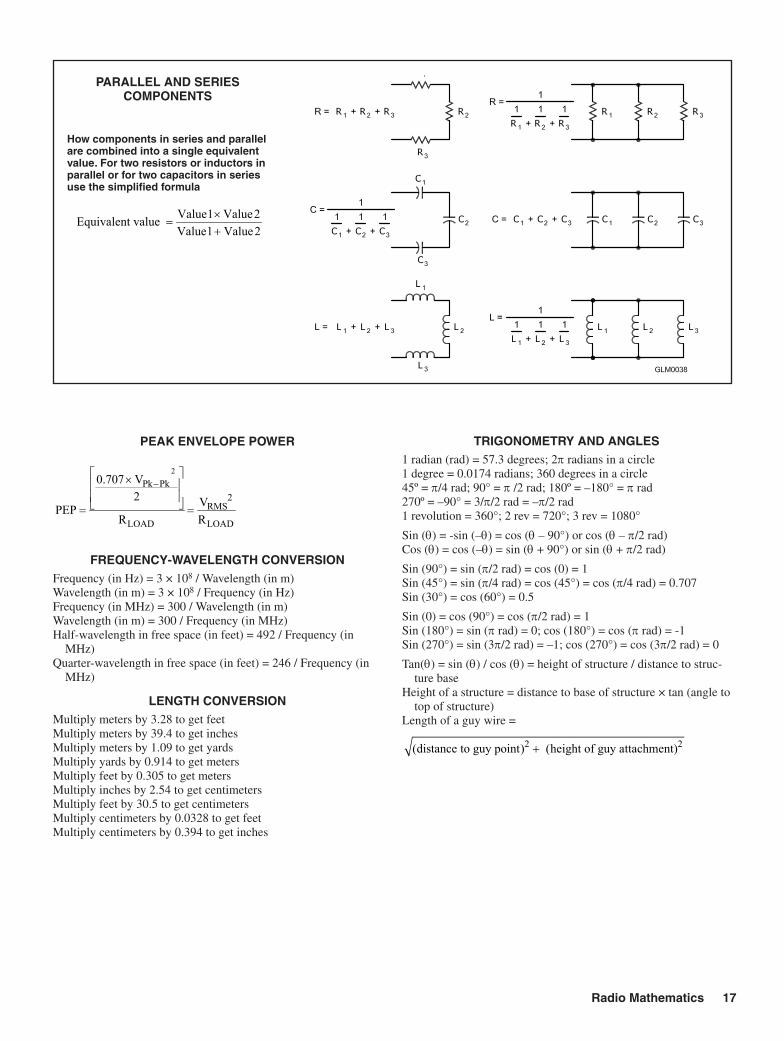
PARALLEL AND SERIES COMPONENTS

How components in series and parallel are combined into a single equivalent value. For two resistors or inductors in parallel or for two capacitors in series use the simplified formula

PEAK ENVELOPE POWER

2

Pk Pk2

RMS

LOAD LOAD

0.707 V2 VPEP

R R

− × = =

FREQUENCY-WAVELENGTH CONVERSIONFrequency (in Hz) = 3 × 108 / Wavelength (in m)Wavelength (in m) = 3 × 108 / Frequency (in Hz)Frequency (in MHz) = 300 / Wavelength (in m)Wavelength (in m) = 300 / Frequency (in MHz)Half-wavelength in free space (in feet) = 492 / Frequency (in

MHz)Quarter-wavelength in free space (in feet) = 246 / Frequency (in

MHz)

LENGTH CONVERSIONMultiply meters by 3.28 to get feetMultiply meters by 39.4 to get inchesMultiply meters by 1.09 to get yardsMultiply yards by 0.914 to get metersMultiply feet by 0.305 to get metersMultiply inches by 2.54 to get centimetersMultiply feet by 30.5 to get centimetersMultiply centimeters by 0.0328 to get feetMultiply centimeters by 0.394 to get inches

Conversion Factors for Sinusoidal AC Voltage or CurrentFrom To Multiply ByPeak Peak-to-Peak 2

Peak-to-Peak Peak 0.5

Peak RMS or 0.707

RMS Peak or 1.414

Peak-to-Peak RMS or 0.35355

RMS Peak-to-Peak or 2.828

Peak Average 2 / π or 0.6366

Average Peak π / 2 or 1.5708

RMS Average or 0.90

Average RMS or 1.11

Note: These conversion factors apply only to continuous pure sine waves.

TRIGONOMETRY AND ANGLES1 radian (rad) = 57.3 degrees; 2π radians in a circle1 degree = 0.0174 radians; 360 degrees in a circle45º = π/4 rad; 90° = π /2 rad; 180º = –180° = π rad270º = –90° = 3/π/2 rad = –π/2 rad1 revolution = 360°; 2 rev = 720°; 3 rev = 1080°

Sin (θ) = -sin (–θ) = cos (θ – 90°) or cos (θ – π/2 rad)Cos (θ) = cos (–θ) = sin (θ + 90°) or sin (θ + π/2 rad)

Sin (90°) = sin (π/2 rad) = cos (0) = 1Sin (45°) = sin (π/4 rad) = cos (45°) = cos (π/4 rad) = 0.707Sin (30°) = cos (60°) = 0.5

Sin (0) = cos (90°) = cos (π/2 rad) = 1Sin (180°) = sin (π rad) = 0; cos (180°) = cos (π rad) = -1Sin (270°) = sin (3π/2 rad) = –1; cos (270°) = cos (3π/2 rad) = 0

Tan(θ) = sin (θ) / cos (θ) = height of structure / distance to struc-ture base

Height of a structure = distance to base of structure × tan (angle to top of structure)

Length of a guy wire =

2 2(distance to guy point) (height of guy attachment)+

Value1 Value2Equivalent value Value1 Value2

×=

+