Basics of Feedback Control Raffaello D’Andrea Mechanical and Aerospace Engineering Cornell University • The importance of understanding dynamics • Open loop versus closed loop control • Shifting sensitivity and uncertainty management • Time scales • Time delays • System coupling • PID control (proportional, integral, derivative control) • State feedback and LQR design (linear/quadratic regulator) FUNDAMENTALS SOME BASIC TOOLS
Transcript
Basics of Feedback ControlRaffaello D’Andrea
Mechanical and Aerospace EngineeringCornell University
• The importance of understanding dynamics• Open loop versus closed loop control• Shifting sensitivity and uncertainty management• Time scales• Time delays• System coupling
• PID control (proportional, integral, derivative control) • State feedback and LQR design (linear/quadratic regulator)
FUNDAMENTALS
SOME BASIC TOOLS
The importance of dynamics...
Isn’t feedback control intuitive?
Raff/RichardForceGenerator
PositionSensor
_+
DESIREDPOSITION
… but seriously, even seemingly simple systems can be difficult to control WITHOUT a basic understandingof the system dynamics.
On the flip side, designing a controller for the Raff/Richard system is very easy to do once you have a model AND somebasic control tools.
Open loop vs. closed loop control...
A Simple Example (No Dynamics!!!)Given the task of designing a power amplifier, desired gain of 1, given the following components:
GAIN BLOCK: DRAWER FULL OF RESISTORS:10 1100 201,000 30010,000 5,000
R = ±= ±= ±= ±
DRAWER FULL OF BASIC INTERCONNECTION COMPONENTS:
1
2
RR
=G
+_
__
++
Straight-forward approach:
10 110 1
±=
±G
Use components with the best relative tolerances!!!
Amplifier Gain = Input/Output Gain: 0.82 < G < 1.22
Variation from desired gain: > 20 %
Design based on feedback:
10,000 5,00010 1
±=
±G
Amplifier Gain: 455 < G < 1,667
_+
Input/Output Gain: 0.9978 < G/(1+G) < 0.9994
Variation from desired gain: < 0.25 %
A component with 50 % error can yield a design with 0.25% error!!!
… incidentally, there are other benefits of the feedback design.Assume G has the following frequency dependence:
0
0
for 0 1,0001,000 for 1,000
G G f
G G ff
= <= <=
= >
•Without feedback, the gain has dropped off by a factor of 2when f=2 kHz.•With feedback, the 3dB frequency will occur when
0.5, 1.0, 1,000*455 455kHz1G G fG= = = =
+
Shifting Sensitivity and Uncertainty Management...
Pr pKo
d 1= ≈o oT PK
Pr pKf
d
F
- = =+
ff o
f
PKT T1 PK F
=−
of
o
KK1 PK F
Design a controller so that the input/output gain is close to 1:
OPEN LOOP:
CLOSED LOOP:
Open Loop Sensitivity
∂ ∂ ∂ ∂= =o o o
o o o
T P T K,T P T K
∂ ∂=f
f
T FF ,T F
Pr pKo
d
Closed Loop Sensitivity
∂ ∂ ∂ ∂= − = −f f f
f f f
T P T K(1 F) , (1 F)T P T K
Pr pKf
d
F
-
•Sensitivity can be shifted: move to less costly, easierto design components.
•There is no free-lunch: sensitivity is in some sensepreserved.
Time Scales...
M=1F
x
Objective: 1) Design a local controller that tracks velocity2) Design a global controller that tracks position
( ), speed of response = v d vF x k v x k= = −1)
( ), "speed of response " = d d d dv k x x k= −
(simplified version of what is used for RoboCup)
2)
Px’
kv F_
+vdx
kd_+xd
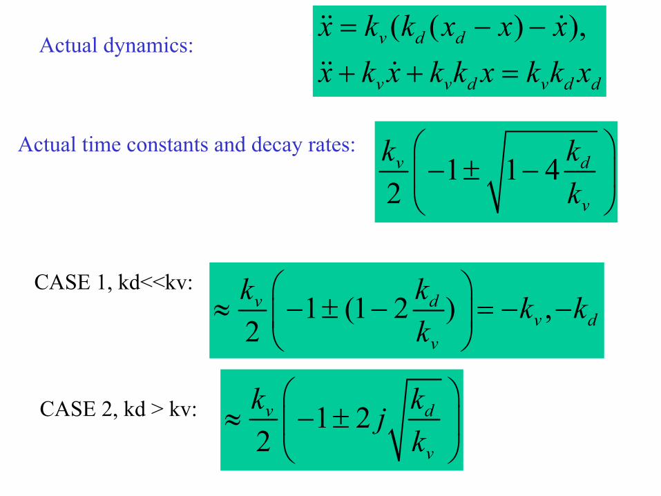
Actual dynamics:( ( ) ),v d d
v v d v d d
x k k x x xx k x k k x k k x= − −+ + =
Actual time constants and decay rates:1 1 4
2v d
v
k kk
− ± −
CASE 1, kd<<kv:1 (1 2 ) ,
2v d
v dv
k k k kk
≈ − ± − = − −
CASE 2, kd > kv: 1 22v d
v
k kjk
≈ − ±
CASE 1:
CASE 2:
Must keep time-scales in mind when designing control systemsfor complex systems.
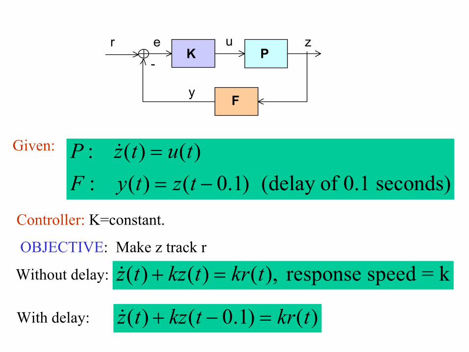
Time Delays...
Pu
Kr
F
-
: ( ) ( ): ( ) ( 0.1) (delay of 0.1 seconds)
P z t u tF y t z t
== −
ze
Given:
y
Controller: K=constant.
OBJECTIVE: Make z track r
Without delay: ( ) ( ) ( ), response speed = kz t kz t kr t+ =
With delay: ( ) ( 0.1) ( )z t kz t kr t+ − =
CASE 1 (k=1):
CASE 2 (k=10):
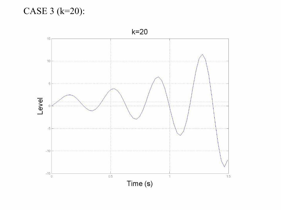
CASE 3 (k=20):
Delayed information has the effect of limiting how quicklywe can control a system.
…turns out that if you have at least 10 of the systems connected,the overall system will be stable.
PID Control...
SOME BASIC TOOLS
PK
d
zuer_
+++
0( ) ( ) ( ) ( )
t
P I Du t k e t k e d k e tτ τ= + +∫
SPEED STEADY STATE PERFORMANCE
STABILITY
ROUGHLY:
kP: the larger the error, the larger the control effort.kI: if system is stable, e(t) must go to zero for constant d(t) and u(t).kD: apply more control effort if error is getting larger.
These interpretations are only rules of thumb: in general,the effects of the gains are dictated by the plant dynamics.
LQR Control...
BACKGROUNDMany systems can be captured by sets of ordinary differential equations:
( ) ( ( ), ( ))( ) ( ( ), ( ))x t f x t u ty t h x t u t
==
• x(t): State of the system, an n-valued vector (x(t)=(x1(t),…xn(t))• u(t): The input to the system, an m-valued vector• y(t): The output of the system, a p-valued vector
If we want to control the system about an operating point (xE,uE), andwe can measure all the states, we can linearize about (xE,uE) to obtain
( ) ( ) ( )( ) ( )x t x t u ty t x t
= +=
A B
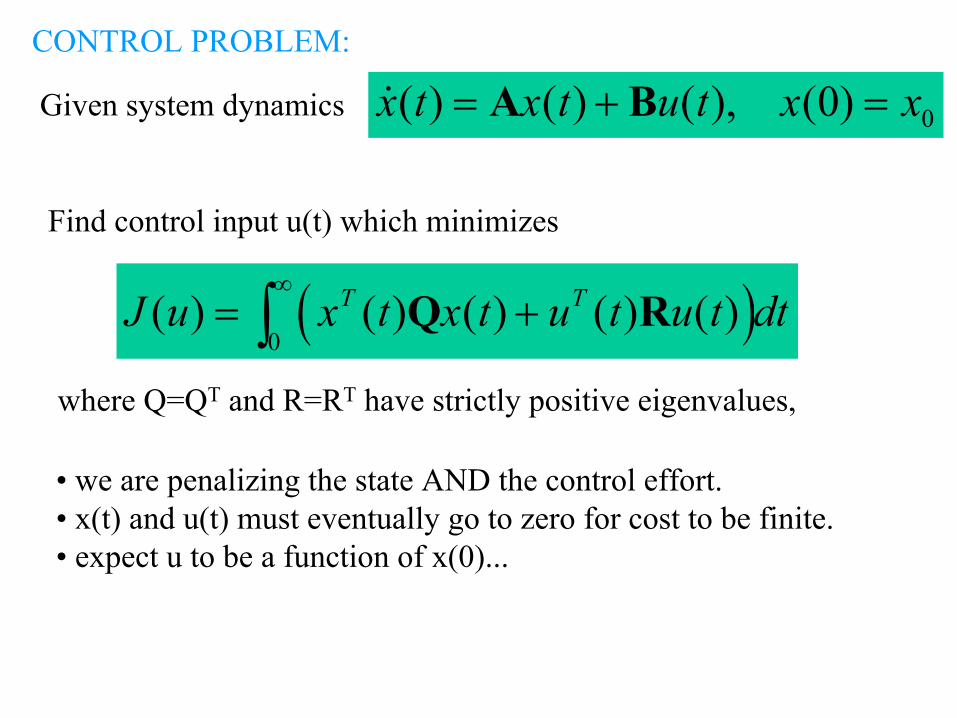
CONTROL PROBLEM:
0( ) ( ) ( ), (0)x t x t u t x x= + =A BGiven system dynamics
Find control input u(t) which minimizes
( )0
( ) ( ) ( ) ( ) ( )T TJ u x t x t u t u t dt∞
= +∫ Q R
• we are penalizing the state AND the control effort.• x(t) and u(t) must eventually go to zero for cost to be finite.• expect u to be a function of x(0)...
where Q=QT and R=RT have strictly positive eigenvalues,
Scalar Case:
( )0
2 2
0
( ) ( ) ( ), (0) ,
( ) ( ) ( )
x t x t u t x x
J u x t u t dt∞
= + =
= +∫
a b
q r
Look for solutions of the form u(t)=kx(t):
0
2 20
( ) exp(( ) ) ,
(assuming 0)2
x t t x
x kJ kk
= +
+= − + < +
a bk
q r a ba b
Minimize J(k): 22 0k k− − + =ar r qb
General Case:
Substitute k=-(b/r)s: 2
2 0ss − + =ba qr
1 0T TS S S S− + =-A + A BR B QAlgebraic Riccati Equation
NOTE:• We restricted our search to u(t)=Kx(t). No obvious reasonwhy this should be the optimal u(t). In fact, we can prove that it is!!!• Unlike most optimal control strategies, the LQR solution is a feedback solution.